Tracking Algorithms for Bistatic Sonar Systems

Martina Daun1 and Frank Ehlers2

1FGAN-FKIE, Dept. Sensor Data and Information FusionWachtberg, GermanyEmail: daun@fgan.de

2 NURC, System Technology DepartmentLa Spezia, Italy

Email: ehlers@nurc.nato.int

Abstract: An active sonar system consists of a sound source activating a surveillancearea and a receiver listening for echoes reflected from targets. In a bistatic setup,the source and the receiver are not collocated. The resulting measurement model isdescribed by a non-linear function of the target state, the given bistatic geometry andenvironmental parameters. For target tracking it is mandatory to have an adequatedescription of the uncertainty on the target state that is resulting from the uncertaintiesin the measurements and environmental parameters. An inadequate description woulddecrease the performance of the fusion process. To cope with the nonlinearity in themeasurement model, four different methods can easily be implemented based on theKalman Filter framework: linear transformation of each measurement in Cartesiancoordinates with tracking in the Cartesian system, unscented transformation of eachmeasurement in Cartesian coordinates with tracking in the Cartesian system, extendedKalman filtering and unscented Kalman filtering. In this paper, we compare thesemethods by simulating their performance in an operationally relevant setup.

1 Introduction

Bistatic sonar has been identified to improve surveillance performance compared to mono-static systems, in particular when exploiting the operational benefit of having a covert re-ceiver. In this setup, the target is loosing the advantage of a stealth design. Operationalconcepts extend this idea also to the ’multistatic setup’ consisting of multiple sources andreceivers. However, due to e.g. communication constraints within the multistatic setup,the pure bistatic scenario has also there an important role: Tracking of contacts from abistatic detection opportunity might lead to tracks which are then sent to a track fusioncentre. The fusion centre collects bistatic tracks from all participating receivers in themultistatic setup. Each bistatic track should be as accurate as possible to ensure at thefusion centre a correct association of received bistatic track information to the same tar-get [GCCG06]. From a system design point of view, the accuracy of measured contactand environmental data is limited by the given variability of the underwater sound channeland by budget or feasibility constraints on the quality and number of measurements. By

precise modelling and calibrating the underwater sound channel the quality of a bistaticsetup can be improved [Cox89]. But in spite of appropriate corrections, some parametersin the multistatic environment may remain imprecise. Thus, from a sequential trackingpoint of view, it is important to correctly model the uncertainties accompanying the actualmeasured values, otherwise the tracking filters are not able to fully exploit the presenteddata.

For bistatic sonar the measurements are described by a non-linear function of the targetstate, the given bistatic geometry and environmental parameters (like the speed of sound,the source and receiver positions and the receiver heading). The measurement model in-cludes noise describing the uncertainty inherent in the measurement process for all ar-guments of this non-linear function. In order to apply sequential tracking techniques inthe framework of a state-space Kalman filter, approximations of the non-linearity and/orits effect on associated uncertainties have to be applied. In [Cor06], measurement uncer-tainties are transformed into Cartesian coordinates by linearizing. We will compare thisapproach with an alternative strategy based on the Unscented Transform (UT) [JU04]. Af-ter the transformation, a linear Kalman filter can be used to track contacts. Two alternativeprocedures are available, known as extended Kalman Filter (EKF) [DP66] and unscentedKalman Filter (UKF) [JU04] that can be adapted to account for uncertainties in the envi-ronmental parameters.

In this paper, we present a performance analysis for these four different methods in termsof Monte Carlo simulations for an operationally relevant bistatic setup, together with acomparison of their tracking results to the Cramer Rao Lower Bound (CRLB) of the asso-ciated estimation problem.

This paper is organized as follows: In the next section the measurement model is described.In section 3 we address the transformation of measurements into Cartesian coordinatesconsidering additional imprecision in the environmental parameters. Different approachesfor Kalman Filtering will be considered in section 4 and finally we discuss the results ofMonte Carlo runs in section 5.

2 Measurement model

The measurement is described as a non-linear function of the target state.

z = h(x) + w, (1)

with Gaussian measurement noise w. The measurement vector has two components:azimuth angle ϕ and time of arrival τ . Let p = (x, y)T be the target position ands = (sx, sy)T and o = (ox, oy)T the position of the source and the receiver respec-tively. The receiver orientation (heading) is given by ϑ, c.f. Fig. 1; then the measurementfunction can be expressed as

ϕ = arctan(

x− ox

y − oy

)− ϑ,

τ = (|p− s|+ |p− o|)/cS ,

(2)

where | · · · | denotes the Euclidian norm and cS is the propagation speed of sound in water.

p

so

p− so− p

−ϕ ϑ

Figure 1: Bistatic Setup; one source, one observer and a single target

3 Mapping of Uncertainties in the Measurements to Cartesian Coor-dinates

According to (2) and Fig. 1, to transform measurement values into x/y coordinates, soundspeed cS , receiver o and source s positions and receiver orientation (heading) ϑ have tobe known. In fact, only estimates of these values will be available. Hence, we model theuncertainty following [BDK08] by

• o ∼ N (o; o,PO)

• s ∼ N (s; s,PS)

• cS ∼ N (cS ; cS , σCS).

An error in the receiver heading can easily be incorporated by enlarging the error in az-imuth information, i.e. if σϕ is the deviation of the measurement error and if σϑ decribesthe uncertainty in the receiver heading, the actual error of the bearing estimate is enlarged

by σϕ =√

σ2ϕ + σ2

ϑ. Noting that the extension to the more sophisticated case is straightforward we set the expected receiver heading to 0◦ in this paper.

This results in a new definition of an artfical measurement vector

za = (τ, ϕ, cS , sT ,oT ). (3)

The 2D-target position x = (x, y) can finally be calculated from

x = g(za), (4)

where we use the following equations:

BL = s− o

α = arctan(BLx/BLy)− ϕ

∆ =√

BL2x + BL2

y

range =(τ · cS)2 −∆2

2(τ · cS −∆ cos(α))

x = sin(ϕ) · range + o(1)

y = cos(ϕ) · range + o(2),

(5)

In [Cor06] a linearization approach has been presented to derive the Cartesian covariancematrix: g is approximated by linearizing. We compare this approach to the UnscentedTransform (UT) [JU04]. The UT delivers the corresponding target state estimate and co-variance matrix by exploiting the relationship given in g. Thus, it provides a very simplemethod to incorporate additional errors.

4 Implementation of the Kalman Filter Scheme

We are interested in investigating effects of additional error sources on Kalman Filtering.The target position estimate derived in the previous section will help us to destine thetrack initialization point. In addition to the target position we initialize target velocitieswith zero mean and deviation of 5m/s in each component.

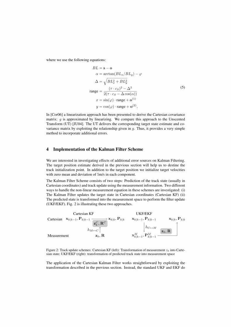
The Kalman Filter Scheme consists of two steps: Prediction of the track state (usually inCartesian coordinates) and track update using the measurement information. Two differentways to handle the non-linear measurement equation in these schemes are investigated: (i)The Kalman Filter updates the target state in Cartesian coordinates (Cartesian KF) (ii)The predicted state is transformed into the measurement space to perform the filter update(UKF/EKF). Fig. 2 is illustrating these two approaches.

Cartesian KFCartesian

Measurement

xk|k−1, Pk|k−1

zCk , RC

zk, R

xk|k, Pk|k

hM 7→C

UKF/EKFxk|k−1, Pk|k−1

xMk|k−1, PM

k|k−1

zk, R

xk|k, Pk|k

hC 7→M

Figure 2: Track update schemes: Cartesian KF (left): Transformation of measurement zk into Carte-sian state; UKF/EKF (right): transformation of predicted track state into measurement space

The application of the Cartesian Kalman Filter works straightforward by exploiting thetransformation described in the previous section. Instead, the standard UKF and EKF do

not care about additional error sources by default, but can easily be transferred by definingthe vector a = (cS ,oT , sT ), containing the environmental parameters. As in the previoussection we can assume the heading vector to be known and pick up the uncertainty in theazimuth uncertainty.

The aim of target tracking is to destine the conditional probability of the target state xk

at time tk given the measurement history Zk = {z1, · · · , zk} and the a priori knowledgeabout the environmental parameters, i.e. a ∼ N (a; a,Ca):

p(xk|Zk,a) ∝ p(zk|a,xk)p(a|xk)p(xk|Zk−1)= N (zk;hC 7→M (xk,a),R)N (a; a,Ca)N (xk;xk|k−1,Pk|k−1)

= N (zk;hC 7→M (xk,a),R)N((

xk

a

);(

xk|k−1

a

),

(Pk|k−1 O

O Ca

)) (6)

The proportionality in the first line holds due to the Bayes rule. Additionally, we exploitthat the measurements do not depend on the measurement history if the target state isknown. According to our assumptions the probability densities can be described by Gaus-sians (line 2), whereas the additional error vector a is independent of the target state. Inthe third line we combine the probability densities regarding target state and system pa-rameter information, i.e. the target state vector is artificially extended, xa = (xT ,aT )T .Thus, the formula shows a good analogy to the standard case (without uncertainties in theenvironmental parameters), i.e. xk is replaced by xa.

Using linearization of the relation given by hC 7→M (xk,a) ≈ H1xk + H2a + b we canexploit the product formula for Gaussian densities and derive the following update formu-las:

xk|k = xk|k−1 + W(zk − h(a,xk))

Pk|k = Pk|k−1 −WSWT ,(7)

where S = H1Pk|k−1HT1 + H2CaHT

2 + R and W = H1Pk|k−1S−1. The updateformulas are very similar to the standard EKF formulas; we abstain from updating theinformation in a, since it is assumed to be independent for different pings. We can easilyreplace the linearization that was used in the derivation by the UT to approximate S andW.

5 Numerical Results of Cartesian Transformation

5.1 Simulation Setup

For numerical evaluation we consider a scenario where the receiver is located at(−1km,0km)T and the source is at (1km,0km)T . Measurement errors are chosen to beσϕ = 2◦, σϑ = 2◦, στ = 0.001s and σcS

= 2m/s. Additionally we assume equal anduncorrelated errors for the components of source and receiver position with σL = 20m,

i.e. PO = PS = diag(σ2L, σ2

L). For this setup the Cartesian transformations (Lineariza-tion/UT) are compared: Results will be presented and discussed in Section 5.2.

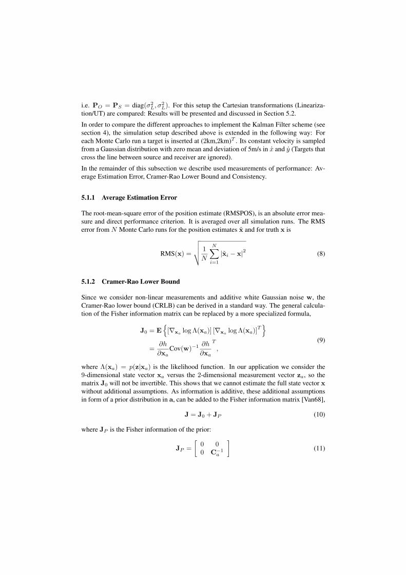
In order to compare the different approaches to implement the Kalman Filter scheme (seesection 4), the simulation setup described above is extended in the following way: Foreach Monte Carlo run a target is inserted at (2km,2km)T . Its constant velocity is sampledfrom a Gaussian distribution with zero mean and deviation of 5m/s in x and y (Targets thatcross the line between source and receiver are ignored).

In the remainder of this subsection we describe used measurements of performance: Av-erage Estimation Error, Cramer-Rao Lower Bound and Consistency.

5.1.1 Average Estimation Error

The root-mean-square error of the position estimate (RMSPOS), is an absolute error mea-sure and direct performance criterion. It is averaged over all simulation runs. The RMSerror from N Monte Carlo runs for the position estimates x and for truth x is

RMS(x) =

√√√√ 1N

N∑i=1

|xi − x|2 (8)

5.1.2 Cramer-Rao Lower Bound

Since we consider non-linear measurements and additive white Gaussian noise w, theCramer-Rao lower bound (CRLB) can be derived in a standard way. The general calcula-tion of the Fisher information matrix can be replaced by a more specialized formula,

J0 = E{

[∇xalog Λ(xa)] [∇xa

log Λ(xa)]T}

=∂h

∂xaCov(w)−1 ∂h

∂xa

T

,(9)

where Λ(xa) = p(z|xa) is the likelihood function. In our application we consider the9-dimensional state vector xa versus the 2-dimensional measurement vector za, so thematrix J0 will not be invertible. This shows that we cannot estimate the full state vector xwithout additional assumptions. As information is additive, these additional assumptionsin form of a prior distribution in a, can be added to the Fisher information matrix [Van68],

J = J0 + JP (10)

where JP is the Fisher information of the prior:

JP =[

0 00 C−1

a

](11)

5.1.3 Consistency

Filter consistency is usually measured using the normalized (state) estimation error squared(NEES), defined as

ε = xT P−1x, (12)

which should be chi-square distributed with ηx degrees of freedom, if the filter is consis-tent. In Monte Carlo simulations that provide N independent samples εi, i = 1, . . . , N ,the average NEES is

ε =1N

N∑i=1

εi. (13)

It has to be tested whether Nε is chi-square distributed with Nηx degrees of freedom. Thishypothesis is accepted, if Nε is in the appropriate acceptance region.

5.2 Comparing Linearization and Unscented Transform

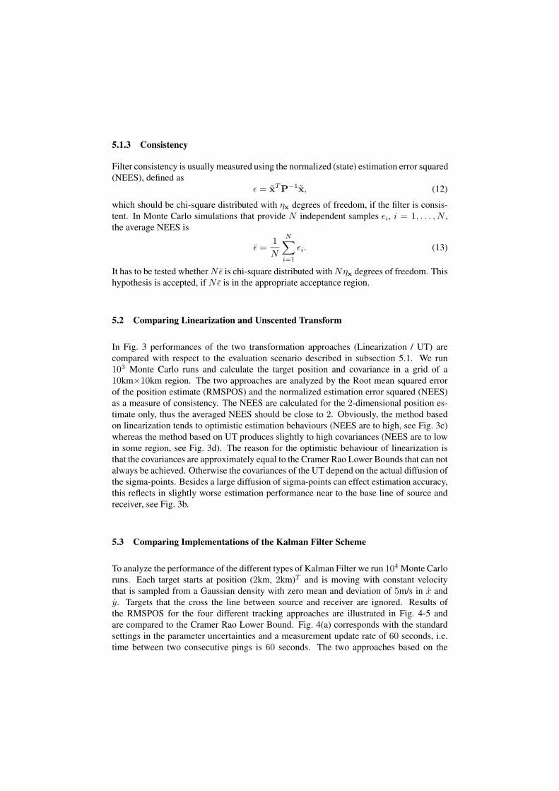
In Fig. 3 performances of the two transformation approaches (Linearization / UT) arecompared with respect to the evaluation scenario described in subsection 5.1. We run103 Monte Carlo runs and calculate the target position and covariance in a grid of a10km×10km region. The two approaches are analyzed by the Root mean squared errorof the position estimate (RMSPOS) and the normalized estimation error squared (NEES)as a measure of consistency. The NEES are calculated for the 2-dimensional position es-timate only, thus the averaged NEES should be close to 2. Obviously, the method basedon linearization tends to optimistic estimation behaviours (NEES are to high, see Fig. 3c)whereas the method based on UT produces slightly to high covariances (NEES are to lowin some region, see Fig. 3d). The reason for the optimistic behaviour of linearization isthat the covariances are approximately equal to the Cramer Rao Lower Bounds that can notalways be achieved. Otherwise the covariances of the UT depend on the actual diffusion ofthe sigma-points. Besides a large diffusion of sigma-points can effect estimation accuracy,this reflects in slightly worse estimation performance near to the base line of source andreceiver, see Fig. 3b.

5.3 Comparing Implementations of the Kalman Filter Scheme

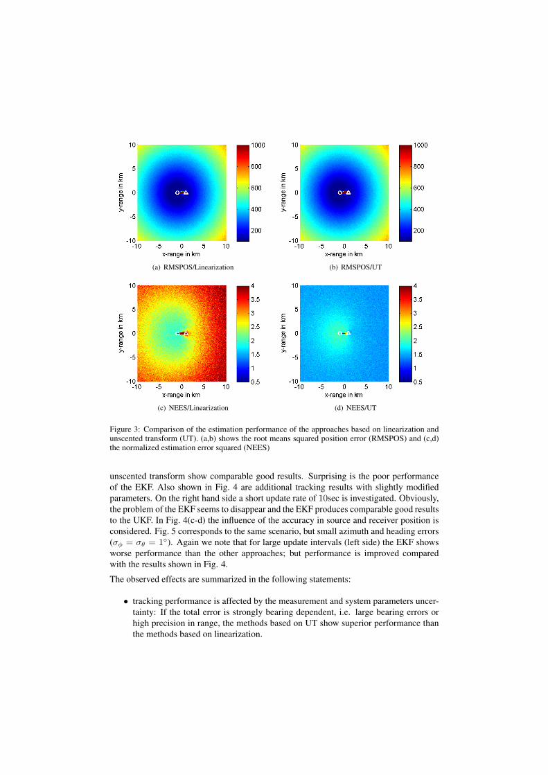
To analyze the performance of the different types of Kalman Filter we run 104 Monte Carloruns. Each target starts at position (2km, 2km)T and is moving with constant velocitythat is sampled from a Gaussian density with zero mean and deviation of 5m/s in x andy. Targets that the cross the line between source and receiver are ignored. Results ofthe RMSPOS for the four different tracking approaches are illustrated in Fig. 4-5 andare compared to the Cramer Rao Lower Bound. Fig. 4(a) corresponds with the standardsettings in the parameter uncertainties and a measurement update rate of 60 seconds, i.e.time between two consecutive pings is 60 seconds. The two approaches based on the

(a) RMSPOS/Linearization (b) RMSPOS/UT

(c) NEES/Linearization (d) NEES/UT

Figure 3: Comparison of the estimation performance of the approaches based on linearization andunscented transform (UT). (a,b) shows the root means squared position error (RMSPOS) and (c,d)the normalized estimation error squared (NEES)

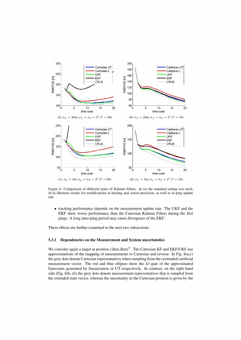
unscented transform show comparable good results. Surprising is the poor performanceof the EKF. Also shown in Fig. 4 are additional tracking results with slightly modifiedparameters. On the right hand side a short update rate of 10sec is investigated. Obviously,the problem of the EKF seems to disappear and the EKF produces comparable good resultsto the UKF. In Fig. 4(c-d) the influence of the accuracy in source and receiver position isconsidered. Fig. 5 corresponds to the same scenario, but small azimuth and heading errors(σφ = σθ = 1◦). Again we note that for large update intervals (left side) the EKF showsworse performance than the other approaches; but performance is improved comparedwith the results shown in Fig. 4.

The observed effects are summarized in the following statements:

• tracking performance is affected by the measurement and system parameters uncer-tainty: If the total error is strongly bearing dependent, i.e. large bearing errors orhigh precision in range, the methods based on UT show superior performance thanthe methods based on linearization.

(a) σL = 20m, σϕ = σϑ = 2◦,T = 60s (b) σL = 20m, σϕ = σϑ = 2◦,T = 10s

(c) σL = 5m, σϕ = σϑ = 2◦,T = 60s (d) σL = 5m, σϕ = σϑ = 2◦,T = 10s

Figure 4: Comparison of different types of Kalman Filters. In (a) the standard setting was used;(b-d) illustrate results for modifications in bearing and sensor precision, as well as in ping updaterate

• tracking performance depends on the measurement update rate: The UKF and theEKF show worse performance than the Cartesian Kalman Filters during the firstpings. A long inter-ping period may cause divergence of the EKF.

These effects are further examined in the next two subsections.

5.3.1 Dependencies on the Measurement and System uncertainties

We consider again a target at position (2km,2km)T . The Cartesian KF and EKF/UKF useapproximations of the mapping of measurements to Cartesian and reverse. In Fig. 6(a,c)the grey dots denote Cartesian representatives when sampling from the (extended) artificialmeasurement vector. The red and blue ellipses show the 3σ-gate of the approximatedGaussians generated by linearization or UT respectively. In contrast, on the right handside (Fig. 6(b, d)) the grey dots denote measurement representatives that is sampled fromthe extended state vector, whereas the uncertainty in the Cartesian position is given by the

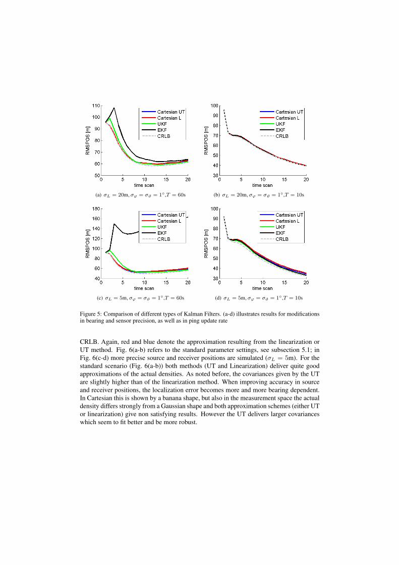
(a) σL = 20m, σϕ = σϑ = 1◦,T = 60s (b) σL = 20m, σϕ = σϑ = 1◦,T = 10s

(c) σL = 5m, σϕ = σϑ = 1◦,T = 60s (d) σL = 5m, σϕ = σϑ = 1◦,T = 10s

Figure 5: Comparison of different types of Kalman Filters. (a-d) illustrates results for modificationsin bearing and sensor precision, as well as in ping update rate

CRLB. Again, red and blue denote the approximation resulting from the linearization orUT method. Fig. 6(a-b) refers to the standard parameter settings, see subsection 5.1; inFig. 6(c-d) more precise source and receiver positions are simulated (σL = 5m). For thestandard scenario (Fig. 6(a-b)) both methods (UT and Linearization) deliver quite goodapproximations of the actual densities. As noted before, the covariances given by the UTare slightly higher than of the linearization method. When improving accuracy in sourceand receiver positions, the localization error becomes more and more bearing dependent.In Cartesian this is shown by a banana shape, but also in the measurement space the actualdensity differs strongly from a Gaussian shape and both approximation schemes (either UTor linearization) give non satisfying results. However the UT delivers larger covarianceswhich seem to fit better and be more robust.

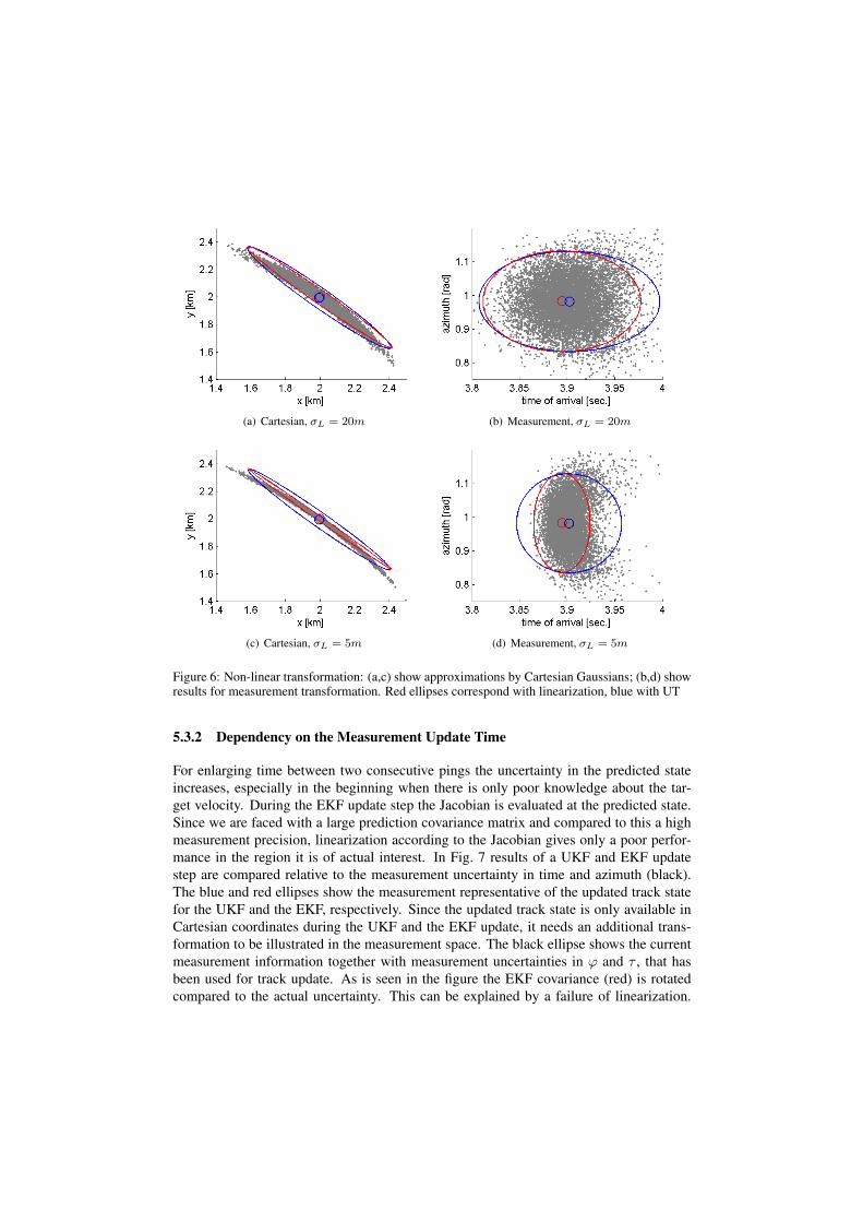
(a) Cartesian, σL = 20m (b) Measurement, σL = 20m

(c) Cartesian, σL = 5m (d) Measurement, σL = 5m

Figure 6: Non-linear transformation: (a,c) show approximations by Cartesian Gaussians; (b,d) showresults for measurement transformation. Red ellipses correspond with linearization, blue with UT

5.3.2 Dependency on the Measurement Update Time

For enlarging time between two consecutive pings the uncertainty in the predicted stateincreases, especially in the beginning when there is only poor knowledge about the tar-get velocity. During the EKF update step the Jacobian is evaluated at the predicted state.Since we are faced with a large prediction covariance matrix and compared to this a highmeasurement precision, linearization according to the Jacobian gives only a poor perfor-mance in the region it is of actual interest. In Fig. 7 results of a UKF and EKF updatestep are compared relative to the measurement uncertainty in time and azimuth (black).The blue and red ellipses show the measurement representative of the updated track statefor the UKF and the EKF, respectively. Since the updated track state is only available inCartesian coordinates during the UKF and the EKF update, it needs an additional trans-formation to be illustrated in the measurement space. The black ellipse shows the currentmeasurement information together with measurement uncertainties in ϕ and τ , that hasbeen used for track update. As is seen in the figure the EKF covariance (red) is rotatedcompared to the actual uncertainty. This can be explained by a failure of linearization.

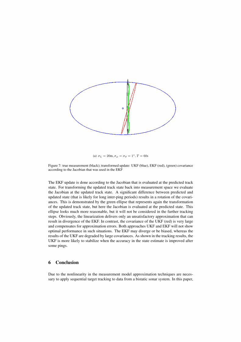
(a) σL = 20m, σϕ = σϑ = 1◦, T = 60s

Figure 7: true measurement (black); transformed update: UKF (blue), EKF (red), (green) covarianceaccording to the Jacobian that was used in the EKF

The EKF update is done according to the Jacobian that is evaluated at the predicted trackstate. For transforming the updated track state back into measurement space we evaluatethe Jacobian at the updated track state. A significant difference between predicted andupdated state (that is likely for long inter-ping periods) results in a rotation of the covari-ances. This is demonstrated by the green ellipse that represents again the transformationof the updated track state, but here the Jacobian is evaluated at the predicted state. Thisellipse looks much more reasonable, but it will not be considered in the further trackingsteps. Obviously, the linearization delivers only an unsatisfactory approximation that canresult in divergence of the EKF. In contrast, the covariance of the UKF (red) is very largeand compensates for approximation errors. Both approaches UKF and EKF will not showoptimal performance in such situations. The EKF may diverge or be biased, whereas theresults of the UKF are degraded by large covariances. As shown in the tracking results, theUKF is more likely to stabilize when the accuracy in the state estimate is improved aftersome pings.

6 Conclusion

Due to the nonlinearity in the measurement model approximation techniques are neces-sary to apply sequential target tracking to data from a bistatic sonar system. In this paper,

we have implemented two approximation techniques, i.e. linearization and the UnscentedTransform, and studied their performance when mapping bistatic data to the Cartesian sys-tem. Especial emphasis lies on incorporating uncertainties inherent in the environmentalparameters. Tracking is possible for both techniques in the Cartesian system. Using alsothe Extended Kalman filter and Unscented Kalman filter schemes, four different trackingmethods are available. We compared their performance based on simulated data, rela-tive to the CRLB. Comparing the approximation techniques linearization and UnscentedTransform, we found that linearization tends to underestimate the actual errors whilst theUnscented Transform tends to overestimate. Referring to tracking performance, UT seemsto be preferable. During the course of the tracking process the accuracy of the target stateestimation is increased (given that the target motion model fits), whereas the accuracy ofthe measurements remains constant (fixed measurement errors). Since the performanceof the approximation seems to depend on the accuracy available in the coordinate systembefore transformation, we propose to switch between approximation techniques: Startingwith tracking in Cartesian coordinates at initialisation phase of a track and then switchingto an UKF (or EKF) scheme.

References

[BDK08] C. R. Berger, M. Daun, and W. Koch. Low Complexity Track Initialization from aSmall Set of Non-Invertible Measurements. EURASIP Journal on Advances in SignalProcessing, 2008.

[Cor06] S. Coraluppi. Multistatic Sonar Localization. IEEE Journal of oceanic engineering,31(4), October 2006.

[Cox89] H. Cox. Fundamentals of active sonar. Underwater acoustic data processing, pages3–24, 1989.

[DP66] W.F. Denham and S. Pines. Sequential Estimation When Measurement Function Non-linearity Is Comparable to Measurement Error. AIAA J., 4(4):1071–1076, 1966.

[GCCG06] O. Gerard, S. Coraluppi, C. Carthel, and D. Grimmett. Benchmark Analysis of NURCMultistatic Tracking Capability. In Proceedings of FUSION Conference, 2006.

[JU04] Simon J. Julier and Jeffrey K. Uhlmann. Unscented Filtering and Nonlinear Estimation.Proceedings of the IEEE, 92(3):401–422, March 2004.

[Van68] H. Van Trees. Detection, Estimation, and Modulation Theory. John Wiley & Sons, Inc.,New York, 1 edition, 1968.