HAL Id: tel-00963601https://tel.archives-ouvertes.fr/tel-00963601

Submitted on 21 Mar 2014

HAL is a multi-disciplinary open accessarchive for the deposit and dissemination of sci-entific research documents, whether they are pub-lished or not. The documents may come fromteaching and research institutions in France orabroad, or from public or private research centers.

L’archive ouverte pluridisciplinaire HAL, estdestinée au dépôt et à la diffusion de documentsscientifiques de niveau recherche, publiés ou non,émanant des établissements d’enseignement et derecherche français ou étrangers, des laboratoirespublics ou privés.

Automatic target recognition using passive bistaticradar signals.Jonathan Pisane

To cite this version:Jonathan Pisane. Automatic target recognition using passive bistatic radar signals.. Other. Supélec;Université de Liège, 2013. English. �NNT : 2013SUPL0009�. �tel-00963601�

Thèse de Doctorat

Domaine: STICSpécialité: Traitement du Signal

Ecole Doctorale "Sciences et Technologies de l’Information,des Télécommunications et des Systèmes"

Présentée par:

Jonathan PISANE

Sujet:

Reconnaissance automatique de ciblespar signaux de radars passifs bistatiques

Automatic target recognitionusing passive bistatic radar signals

Soutenue le 04 avril 2013 devant les membres du jury:

M. Sylvain Azarian SONDRA, SUPELEC EncadrantM. René Garello Telecom-Bretagne RapporteurM. Hugh Griffiths University College London ExaminateurM. Marc Lesturgie ONERA/SONDRA, SUPELEC Directeur de thèseM. Xavier Neyt Royal Military Academy RapporteurM. Jacques Verly University of Liège Directeur de thèseM. Luc Vignaud ONERA ExaminateurM. Eric Walter SUPELEC ExaminateurM. Louis Wehenkel University of Liège Examinateur

©Copyright Université de Liège©Copyright SUPELEC - Paris XI

Abstract

We present the design, development, and test of three novel, distinct automatic targetrecognition (ATR) systems for the recognition of airplanes and, more specifically, non-cooperative airplanes, i.e. airplanes that do not provide information when interrogated,in the framework of passive bistatic radar systems. Passive bistatic radar systems useone or more illuminators of opportunity (already present in the field), with frequenciesup to 1 GHz for the transmitter part of the systems considered here, and one or morereceivers, deployed by the persons managing the system, and not co-located with thetransmitters. The sole source of information are the signal scattered on the airplaneand the direct-path signal that are collected by the receiver, some basic knowledgeabout the transmitter, and the geometrical bistatic radar configuration.The three distinct ATR systems that we built respectively use the radar images, thebistatic complex radar cross-section (BS-RCS), and the bistatic radar cross-section (BS-RCS) of the targets. We use data acquired either on scale models of airplanes placed inan anechoic, electromagnetic chamber or on real-size airplanes using a bistatic testbedconsisting of a VOR transmitter and a software-defined radio (SDR) receiver, locatednear Orly airport, France.We describe the radar phenomenology pertinent for the problem at hand, as well asthe mathematical underpinnings of the derivation of the bistatic RCS values and of theconstruction of the radar images.For the classification of the observed targets into pre-defined classes, we use eitherextremely randomized trees or subspace methods. A key feature of our approach isthat we break the recognition problem into a set of sub-problems by decomposing theparameter space, which consists of the frequency, the polarization, the aspect angle,and the bistatic angle, into regions. We build one recognizer for each region.We first validate the extra-trees method on the radar images of the MSTAR dataset,featuring ground vehicles. We then test the method on the images of the airplanesconstructed from data acquired in the anechoic chamber, achieving a probability ofcorrect recognition up to 0.99.We test the subspace methods on the BS-CRCS and on the BS-RCS of the airplanesextracted from the data acquired in the anechoic chamber, achieving a probability ofcorrect recognition up to 0.98, with variations according to the frequency band, thepolarization, the sector of aspect angle, the sector of bistatic angle, and the number of(Tx,Rx) pairs used.The ATR system deployed in the field gives a probability of correct recognition of 0.82,with variations according to the sector of aspect angle and the sector of bistatic angle.

Keywords: Automatic target recognition (ATR), non-cooperative target recogni-tion (NCTR), classification, extremely randomized trees (extra-trees), subspace, pas-sive radar, bistatic radar, radar cross-section, complex radar cross-section, illuminatorof opportunity, VOR, software-defined radio (SDR), airplanes, anechoic chamber, airtraffic control.

i

Acknowledgements

This work could not have been performed without the contributions of variouspersons. These persons all guided me and supported me at some time along my work.

In particular, I wish to thank my two supervisors, Marc Lesturgie, Director ofthe SONDRA lab of SUPELEC, and Jacques Verly, Professor in the Department ofElectricity, Electronics, and Computer Science of the University of Liège, for havingaccepted to coach me during this thesis. Their advice throughout the entire durationof the thesis was invaluable. I really enjoyed the various discussions we have had,whether technical or not. I hope they have made me a better scientist, a betterengineer, and a better person.

I also wish to express my deepest gratitude to Sylvain Azarian for his technicaladvice throughout the last two years of the thesis, and for his various comments thathelped me make this manuscript clearer. I also thank him for his invaluable helpduring the experiments that could not have been performed without him. I also wish tothank Raphaël Marée for the various discussions we have had on the different classifi-cation techniques, and for his help in understanding extra-trees and the PiXiT software.

I wish to thank Professor Garello, Professor Griffiths, Professor Neyt, DoctorVignaud, Doctor Walter, and Professor Wehenkel for having accepted to be part ofmy jury. I am really grateful for the interest they show for my work.

During this thesis, I have had the opportunity to work both at the SONDRA lab ofSUPELEC, and among the Department of Electricity, Electronics, and Computer Sci-ence of the University of Liège. Let the people of these two entities be thanked for thenice time I have enjoyed with them. I have had a particularly great time with FrédéricBrigui, Chin Yuan Chong, Jacques El-Khoury, Jérôme Euzière, Pierre Formont, IsraëlHinostroza, Mélanie Mahot, Azza Mokadem, and Danny Tan at SONDRA, and withNicolas Crosset, Géraldine Guerri, Samuel Hiard, Nicolas Marchal, François Schnitzler,and Xavier Werner at the University of Liège. I also wish to thank all the PhD studentsof the "Réseau des Doctorants" of the University of Liège for the projects we didtogether, especially the 2009 "Rentrée des Doctorants" and the discussions we have had.

During these four years, I have had the opportunity to coach several MS thesesat the University of Liège, in the context of the OUFTI-1 project. Since I believethis experience has enriched me, I would like to thank all the members of such a niceproject, and the different students I tried to guide the best I could.

I also wish to thank Anne-Hélène Picot at SONDRA and Marie-Berthe Lecomte,Danielle Bonten, and Sandrine Lovinfosse at the University of Liège for having madethe administrative side of my thesis easier to deal with.

Let me also thank the Belgian National Fund for Scientific Research (FRS-FNRS)for having granted me a scholarship of the Fund for Research in Industry andAgriculture (FRIA) during these fours years.

iii

A thesis requires a huge amount of personal involvement. I wish to thank allmy friends and family, especially Amandine and my parents, for their kindness andunderstanding during these four years, and especially during the writing of thismanuscript.

Finally, I wish to thank all the persons I forgot to mention here.

iv

Table of Contents

Page

Abstract i

Acknowledgements iii

Résumé xi

1 Introduction 11.1 Motivation for the thesis . . . . . . . . . . . . . . . . . . . . . . . . . . 1

1.1.1 Targets considered . . . . . . . . . . . . . . . . . . . . . . . . . 21.1.2 Automatic target recognition (ATR) . . . . . . . . . . . . . . . 21.1.3 Class of a target . . . . . . . . . . . . . . . . . . . . . . . . . . 31.1.4 Bistatic radar . . . . . . . . . . . . . . . . . . . . . . . . . . . . 31.1.5 Passive radar . . . . . . . . . . . . . . . . . . . . . . . . . . . . 3

1.2 Developed techniques . . . . . . . . . . . . . . . . . . . . . . . . . . . . 51.2.1 Scene parameters . . . . . . . . . . . . . . . . . . . . . . . . . . 51.2.2 Quantities used for the recognition of targets . . . . . . . . . . . 61.2.3 Proposed ATR systems . . . . . . . . . . . . . . . . . . . . . . . 6

1.3 Background: conventional air traffic control (ATC) . . . . . . . . . . . 81.3.1 Primary surveillance radar . . . . . . . . . . . . . . . . . . . . . 91.3.2 Secondary surveillance radar . . . . . . . . . . . . . . . . . . . . 101.3.3 Non-cooperative target recognition within ATC . . . . . . . . . 11

1.4 Contributions of the thesis . . . . . . . . . . . . . . . . . . . . . . . . . 111.5 Organization of the manuscript . . . . . . . . . . . . . . . . . . . . . . 121.6 Conclusion . . . . . . . . . . . . . . . . . . . . . . . . . . . . . . . . . . 13

2 PBR, illuminators of opportunity, and ATR: state-of-art 152.1 Passive bistatic radar . . . . . . . . . . . . . . . . . . . . . . . . . . . . 152.2 Illuminators of opportunity . . . . . . . . . . . . . . . . . . . . . . . . 162.3 Automatic target recognition (ATR) . . . . . . . . . . . . . . . . . . . 17

2.3.1 Canonical block diagram of a conventional ATR system . . . . . 172.3.2 Adaptation of the canonical block diagram to our problem . . . 182.3.3 Input data and classification techniques of ATR systems . . . . 18

2.4 Conclusion . . . . . . . . . . . . . . . . . . . . . . . . . . . . . . . . . . 21

3 Bistatic radar phenomenology 233.1 Motivation . . . . . . . . . . . . . . . . . . . . . . . . . . . . . . . . . . 243.2 Notations . . . . . . . . . . . . . . . . . . . . . . . . . . . . . . . . . . 243.3 Bistatic scattering geometry . . . . . . . . . . . . . . . . . . . . . . . . 24

v

3.4 Definition of the BS-CRCS and the BS-RCS . . . . . . . . . . . . . . . 263.5 Scattering mechanisms . . . . . . . . . . . . . . . . . . . . . . . . . . . 273.6 Scattering regions . . . . . . . . . . . . . . . . . . . . . . . . . . . . . . 303.7 BS-RCS of a perfectly conducting sphere . . . . . . . . . . . . . . . . . 31

3.7.1 Hypotheses . . . . . . . . . . . . . . . . . . . . . . . . . . . . . 323.7.2 Transmitted electric and magnetic fields . . . . . . . . . . . . . 333.7.3 Scattered electric field . . . . . . . . . . . . . . . . . . . . . . . 353.7.4 BS-CRCS and BS-RCS as a function of the bistatic angle . . . . 383.7.5 Application to the case of the perfectly conducting sphere . . . 403.7.6 BS-RCS of canonical objects . . . . . . . . . . . . . . . . . . . . 41

3.8 Monostatic-to-bistatic equivalence theorems . . . . . . . . . . . . . . . 423.9 Conclusion . . . . . . . . . . . . . . . . . . . . . . . . . . . . . . . . . . 42

4 Extraction and illustrations of the bistatic RCS of targets 454.1 Motivation . . . . . . . . . . . . . . . . . . . . . . . . . . . . . . . . . . 464.2 Extraction of the BS-CRCS and the BS-RCS of targets . . . . . . . . . 47

4.2.1 Transmitted electric field . . . . . . . . . . . . . . . . . . . . . . 474.2.2 Polarization . . . . . . . . . . . . . . . . . . . . . . . . . . . . . 484.2.3 Expressions for the Tx and Rx E-fields . . . . . . . . . . . . . . 504.2.4 Bistatic polarization scattering matrix . . . . . . . . . . . . . . 524.2.5 Components of the bistatic polarization scattering matrix . . . . 534.2.6 Bistatic complex RCS . . . . . . . . . . . . . . . . . . . . . . . 554.2.7 Bistatic polarization CRCS matrix . . . . . . . . . . . . . . . . 564.2.8 Position of the Tx as reference for the Tx electric field . . . . . . 574.2.9 Case of a single linear polarization . . . . . . . . . . . . . . . . 584.2.10 Practical measurement of the BS-RCS of targets . . . . . . . . . 59

4.3 Acquisition of raw data: experimental setup . . . . . . . . . . . . . . . 594.3.1 Motivation for using scaled models in an anechoic chamber . . . 594.3.2 Configuration geometry . . . . . . . . . . . . . . . . . . . . . . 604.3.3 Acquisition of raw data . . . . . . . . . . . . . . . . . . . . . . . 614.3.4 Airplanes of interest . . . . . . . . . . . . . . . . . . . . . . . . 63

4.4 Scattering regions . . . . . . . . . . . . . . . . . . . . . . . . . . . . . . 654.5 Classes of airplanes . . . . . . . . . . . . . . . . . . . . . . . . . . . . . 654.6 Illustration of the BS-CRCS and the BS-RCS of targets . . . . . . . . . 66

4.6.1 BS-CRCS as a function of the bistatic angle . . . . . . . . . . . 664.6.2 BS-CRCS as a function of the frequency . . . . . . . . . . . . . 694.6.3 BS-CRCS as a function of the polarization . . . . . . . . . . . . 734.6.4 BS-CRCS as a function of the orientation . . . . . . . . . . . . . 734.6.5 Conclusions about the variations of BS-CRCS . . . . . . . . . . 75

4.7 Conclusion . . . . . . . . . . . . . . . . . . . . . . . . . . . . . . . . . . 77

5 Construction of radar images 795.1 Motivation . . . . . . . . . . . . . . . . . . . . . . . . . . . . . . . . . . 795.2 Review of tomographic imaging . . . . . . . . . . . . . . . . . . . . . . 80

5.2.1 The Radon Transform . . . . . . . . . . . . . . . . . . . . . . . 805.2.2 The 2DFT and its rotation property . . . . . . . . . . . . . . . 805.2.3 The projection-slice theorem . . . . . . . . . . . . . . . . . . . . 82

5.3 Principles of monostatic radar imaging . . . . . . . . . . . . . . . . . . 845.3.1 Monostatic (MS) configuration . . . . . . . . . . . . . . . . . . 84

vi

5.3.2 Monostatic (MS) radar imaging . . . . . . . . . . . . . . . . . . 845.4 Principles of bistatic radar imaging . . . . . . . . . . . . . . . . . . . . 87

5.4.1 Bistatic (BS) configuration . . . . . . . . . . . . . . . . . . . . . 875.4.2 Bistatic (BS) imaging . . . . . . . . . . . . . . . . . . . . . . . . 88

5.5 Practical construction of bistatic radar images . . . . . . . . . . . . . . 905.6 Examples of constructed radar images . . . . . . . . . . . . . . . . . . . 945.7 Conclusion . . . . . . . . . . . . . . . . . . . . . . . . . . . . . . . . . . 97

6 Recognition of targets by using their radar images 996.1 Motivation . . . . . . . . . . . . . . . . . . . . . . . . . . . . . . . . . . 1006.2 Physical and parameter spaces . . . . . . . . . . . . . . . . . . . . . . . 101

6.2.1 Physical space . . . . . . . . . . . . . . . . . . . . . . . . . . . . 1016.2.2 Parameter space . . . . . . . . . . . . . . . . . . . . . . . . . . 105

6.3 Recognition strategy . . . . . . . . . . . . . . . . . . . . . . . . . . . . 1066.4 Block diagram of the recognizer . . . . . . . . . . . . . . . . . . . . . . 1116.5 Production of feature vectors by window extraction . . . . . . . . . . . 1126.6 Determination of target class model by extra-trees . . . . . . . . . . . . 113

6.6.1 Deterministic decision tree . . . . . . . . . . . . . . . . . . . . . 1136.6.2 Extremely randomized trees . . . . . . . . . . . . . . . . . . . . 1146.6.3 Motivation for using extremely randomized trees . . . . . . . . . 115

6.7 Determination of the target class . . . . . . . . . . . . . . . . . . . . . 1166.8 Quantification of performance . . . . . . . . . . . . . . . . . . . . . . . 1166.9 Recognition experiments on MSTAR images . . . . . . . . . . . . . . . 117

6.9.1 Description of MSTAR images . . . . . . . . . . . . . . . . . . . 1176.9.2 Experimental sets of images . . . . . . . . . . . . . . . . . . . . 1176.9.3 Parameters of the recognizer . . . . . . . . . . . . . . . . . . . . 1206.9.4 Recognition results . . . . . . . . . . . . . . . . . . . . . . . . . 120

6.10 Recognition experiments on ONERA images . . . . . . . . . . . . . . . 1276.10.1 Experimental sets of images . . . . . . . . . . . . . . . . . . . . 1276.10.2 Parameters of the recognizer . . . . . . . . . . . . . . . . . . . . 1286.10.3 Recognition results . . . . . . . . . . . . . . . . . . . . . . . . . 128

6.11 Conclusion . . . . . . . . . . . . . . . . . . . . . . . . . . . . . . . . . . 136

7 Recognition of targets by using their bistatic RCS or CRCS 1397.1 Motivation . . . . . . . . . . . . . . . . . . . . . . . . . . . . . . . . . . 1407.2 Block diagram of the recognizer . . . . . . . . . . . . . . . . . . . . . . 1417.3 Production of feature vectors . . . . . . . . . . . . . . . . . . . . . . . 1427.4 Determination of target class model by vector spaces . . . . . . . . . . 143

7.4.1 Motivation for using subspace methods . . . . . . . . . . . . . . 1437.4.2 Subspaces . . . . . . . . . . . . . . . . . . . . . . . . . . . . . . 1437.4.3 Size of subspaces . . . . . . . . . . . . . . . . . . . . . . . . . . 145

7.5 Determination of the target class . . . . . . . . . . . . . . . . . . . . . 1457.5.1 Orthogonal projection . . . . . . . . . . . . . . . . . . . . . . . 1467.5.2 Metrics . . . . . . . . . . . . . . . . . . . . . . . . . . . . . . . 1477.5.3 Oblique projection . . . . . . . . . . . . . . . . . . . . . . . . . 148

7.6 Quantification of performance . . . . . . . . . . . . . . . . . . . . . . . 1487.7 Recognition experiments . . . . . . . . . . . . . . . . . . . . . . . . . . 149

7.7.1 Experimental sets . . . . . . . . . . . . . . . . . . . . . . . . . . 1497.7.2 Recognition results achieved for a single (Tx,Rx) pair . . . . . . 149

vii

7.7.3 Recognition results achieved for three (Tx,Rx) pairs . . . . . . . 1637.8 Conclusion . . . . . . . . . . . . . . . . . . . . . . . . . . . . . . . . . . 167

8 Recognition of targets by using their real-life bistatic RCS 1698.1 Motivation . . . . . . . . . . . . . . . . . . . . . . . . . . . . . . . . . . 1708.2 Block diagram of the ATR system . . . . . . . . . . . . . . . . . . . . . 1718.3 Detection, discrimination, and pre-classification . . . . . . . . . . . . . 1718.4 Classes of targets . . . . . . . . . . . . . . . . . . . . . . . . . . . . . . 172

8.4.1 Types of detected airplanes . . . . . . . . . . . . . . . . . . . . 1728.4.2 Grouping of targets into classes . . . . . . . . . . . . . . . . . . 174

8.5 Scene parameters . . . . . . . . . . . . . . . . . . . . . . . . . . . . . . 1768.6 Extraction of the BS-RCS . . . . . . . . . . . . . . . . . . . . . . . . . 176

8.6.1 Extraction of the BS-RCS from real-life data . . . . . . . . . . . 1768.6.2 Generation of the BS-RCS from a simple model . . . . . . . . . 180

8.7 Recognition stage . . . . . . . . . . . . . . . . . . . . . . . . . . . . . . 1808.8 Experimental setup . . . . . . . . . . . . . . . . . . . . . . . . . . . . . 181

8.8.1 Testbed . . . . . . . . . . . . . . . . . . . . . . . . . . . . . . . 1818.8.2 The VOR as a simple illuminator of opportunity . . . . . . . . . 1818.8.3 Collecting the received signals by an SDR receiver . . . . . . . . 1838.8.4 Digital processing of received signals . . . . . . . . . . . . . . . 183

8.9 Data collected and examples of received signals . . . . . . . . . . . . . 1848.9.1 Data available for our recognition experiments . . . . . . . . . . 1848.9.2 Received ADS-B data . . . . . . . . . . . . . . . . . . . . . . . 1858.9.3 Spectrograms . . . . . . . . . . . . . . . . . . . . . . . . . . . . 1858.9.4 Signal-to-noise-ratios . . . . . . . . . . . . . . . . . . . . . . . . 1878.9.5 Variations of the BS-RCS as a function of time . . . . . . . . . 1898.9.6 Distributions of the BS-RCS in (α, β) plane . . . . . . . . . . . 189

8.10 Errors on position, bistatic angle, and BS-RCS . . . . . . . . . . . . . . 1938.10.1 Error on the position of a target . . . . . . . . . . . . . . . . . . 1938.10.2 Influence of the error in position on the bistatic RCS . . . . . . 1938.10.3 Reasons for using the BS-RCS instead of the BS-CRCS . . . . . 196

8.11 Recognition experiments performed . . . . . . . . . . . . . . . . . . . . 1968.11.1 Amount of data . . . . . . . . . . . . . . . . . . . . . . . . . . . 1978.11.2 Statistics of the feature vectors and brief analysis thereof . . . . 2028.11.3 Recognition results for the three-class experiment . . . . . . . . 2028.11.4 Recognition results for all four recognition experiments . . . . . 208

8.12 Conclusion . . . . . . . . . . . . . . . . . . . . . . . . . . . . . . . . . . 208

9 Conclusions and perspectives 2119.1 Conclusions . . . . . . . . . . . . . . . . . . . . . . . . . . . . . . . . . 211

9.1.1 Summary of the thesis . . . . . . . . . . . . . . . . . . . . . . . 2119.1.2 Comparison of the performances of the three ATR systems . . . 213

9.2 Perspectives . . . . . . . . . . . . . . . . . . . . . . . . . . . . . . . . . 2149.2.1 Addition of different types of targets . . . . . . . . . . . . . . . 2159.2.2 Study of bistatic radar phenomenology . . . . . . . . . . . . . . 2159.2.3 Use of different illuminators of opportunity . . . . . . . . . . . . 2159.2.4 Refinement of the recognizer . . . . . . . . . . . . . . . . . . . . 216

Appendices 219

viii

A Confusion matrices for the recognition using real-life BS-RCS 221

B Publications 2312.1 Journal articles . . . . . . . . . . . . . . . . . . . . . . . . . . . . . . . 2312.2 Conference papers . . . . . . . . . . . . . . . . . . . . . . . . . . . . . . 2312.3 Other publications . . . . . . . . . . . . . . . . . . . . . . . . . . . . . 232

Bibliography 233

ix

x

Résumé

I Introduction

I.1 Problème à traiter

Dans cette thèse, nous étudions le problème de la reconnaissance automatiquede cibles en utilisant des signaux de radars passifs bistatiques, afin de détecter desanomalies dans le trafic aérien civil. Les cibles considérées sont donc des avions.

Dans cette section, nous décrivons d’abord le fonctionnement du contrôle du traficaérien civil, et expliquons les raisons pour lesquelles des anomalies peuvent se produire.Nous présentons ensuite la solution que l’on implémente, et en particulier, les différentsconcepts que sont les radars passif bistatiques et la reconnaissance automatique decibles.

I.2 Contexte: le contrôle du trafic aérien civil

Le trafic aérien civil est contrôlé par deux types de radars: les radars primaireset les radars secondaires. Les radars primaires détectent la présence d’avions. Ilsémettent un signal qui est réfléchi sur les avions. Par calcul à partir du signal réfléchi,ils détectent et localisent les avions.

Les radars secondaires servent à l’identification des avions. Les radars secondairesinterrogent les transpondeurs des avions, et ceux-ci leur répondent en envoyant desinformations telles que leur identification ICAO et leur position acquise par GPS.

L’identification d’avions requiert donc un radar secondaire et un transpondeur debord. Des avions tels que les petits avions personnels n’étant pas équipés de telstranspondeurs, leur identification n’est pas garantie par des radars secondaires. Pourreconnaitre des avions, nous utilisons, dans cette thèse, des radars passifs bistatiques.

I.3 Solution au problème posé

Nous procédons à la reconnaissance des avions, appelés cibles, par l’utilisation designaux de radars passifs bistatiques. Le schéma de la figure 1 représente une situationréaliste du problème traité. Un avion inconnu est illuminé par le signal émis par unémetteur d’opportunité. Ce signal est réfléchi par l’avion, et acquis par un récepteur.Le système de reconnaissance automatique de cibles (RAC) détermine ensuite la classede l’avion sur base de ce signal réfléchi.

xi

Les classes des avions à reconnaitre sont définies sur la base des caractéristiquesphysiques de ces avions (aspect et taille). Par exemple, deux avions de même taillese verront attribuer la même classe, même s’ils sont de marques et/ou de compagniesaériennes différentes.

Figure 1: Configuration du système de RAC par radar passif bistatique servant àdéterminer la classe de l’avion.

Un radar bistatique se caractérise par le fait que l’émetteur (Tx) et le récepteur(Rx) ne sont pas co-localisés, comme représenté à la figure 2. L’angle bistatique βest un paramètre-clé de la configuration bistatique. Un radar est dit passif quandl’émetteur utilisé est déjà présent dans l’environnement, et n’est pas conçu ni utiliséspécifiquement à des fins de radar. Les émetteurs de radio FM sont un exempled’émetteur d’opportunité.

A partir du signal réfléchi par un avion et acquis par le récepteur, la surfaceéquivalente radar, complexe (SERC) ou réelle (SER), de cet avion peut être calculée.L’image radar de cet avion peut être construite à partir de sa SERC. Chacun destrois systèmes RAC que nous discutons dans cette thèse se base sur une de cestrois quantités. La système RAC utilisant l’image radar des avions est discuté à lasection III, celui utilisant la SERC ou la SER acquise à partir de mesures en chambreanéchoïque est discuté à la section IV, et celui utilisant la SER acquise à partir demesures en extérieur est discuté à la section V.

Dans cette thèse, nous nous plaçons dans le contexte de l’apprentissage supervisé,c’est-à-dire que le nombre de classes est connu au préalable, et que des données(images, SERC ou SER) pour chacune de ces classes sont disponibles, tant au moment

xii

β

Avion

Tx Rx

Figure 2: Illustration de la configuration bistatique.

de la construction du modèle de reconnaissance que du test de ce modèle. La figure 3montre le bloc-diagramme schématique de l’étage de reconnaissance d’un systèmeRAC. Les données sont séparées en un ensemble d’apprentissage (LS) et un ensemblede test (TS). Un certain nombre de vecteurs d’attributs sont extraits des données dechaque ensemble. Les vecteurs d’attributs du LS servent à construire un modèle dereconnaissance/classification qui est ensuite testé sur les vecteurs d’attributs du TS.

Figure 3: Bloc-diagramme de l’étage de reconnaissance des systèmes RAC.

Deux techniques de classification sont utilisées dans cette thèse; le modèle de re-connaissance consiste soit en un ensemble d’arbres de décision rendus extrêmementaléatoires (extra-trees), soit en un ensemble de sous-espaces vectoriels. Chacun destrois systèmes RAC utilise l’une ou l’autre de ces deux méthodes de classification.

I.4 Organisation du résumé

Le présent résumé est organisé comme suit. La section II résume les concepts dephénoménologie importants pour le problème traité, ainsi que la stratégie de recon-naissance que nous définissons à partir de la phénoménologie radar bistatique. Lasection III discute le système RAC basé sur les images des avions. La section IV dis-cute le système RAC basé sur les SERC et les SER des avions acquises en chambre

xiii

anéchoïque. La section V discute le système RAC basé sur les SER d’avions acquisespar un banc expérimental déployé dans le cadre de cette thèse. La section VI conclutle travail et résume les perspectives envisagées.

II Phénoménologie radar bistatique et stratégie de

reconnaissance

Les trois systèmes de reconnaissance automatique de cibles (RAC) discutés dansles sections suivantes se basent sur la notion de surface équivalente radar, complexe(SERC) ou réelle (SER). Nous présentons dans cette section les éléments-clés de laphénoménologie radar bistatique qui nous permettent de définir une stratégie de re-connaissance.

II.1 Surface équivalente radar complexe et réelle

La figure 4 représente la géométrie d’une configuration bistatique. La cible illuminéeest située au centre d’un repère orthonormé. L’émetteur est situé au point T et lerécepteur au point R, à des distances respectives rT et rR de la cible. Les polarisationsde l’émetteur et du récepteur sont respectivement notées par θT et φ

T, et par θR, φ

R.

b b

b

T

R

P

φ

θ

rP

y

z

x

rR

rT

Cible

β

OkT

φT

θT

θR

φR

rT

rR = kR

rP

p

p

p

p

Figure 4: Géométrie de la configuration bistatique considérée.

La surface équivalente radar réelle (SER) d’un objet, ici la cible, dénotée par σ,est définie dans la littérature comme étant la mesure de l’énergie d’un signal qui estréfléchie par cet objet dans la direction du récepteur. On l’exprime comme

σ = limrR→∞

4πr2R

|Er(rR)|2

|Et(0)|2

, (1)

où rR est la distance entre l’objet et le récepteur, Er(rR) le champ électrique au

récepteur, et Et(0) le champ électrique transmis à la cible.

xiv

La surface équivalente radar complexe (SERC) d’un objet, dénotée par√σ, est

définie dans la littérature par

√σ = lim

rR→∞2√πrR

Er(rR)

Et(0)

ejkrR, (2)

avec les mêmes notations que pour la définition de la SER σ.

La littérature montre que, pour une configuration bistatique, la SERC et la SERd’un objet dépendent de quatre facteurs: la fréquence f du signal illuminant l’objet,le couple Pol de polarisations de l’émetteur et du récepteur, l’angle d’aspect α, etl’angle bistatique β. La figure 5 illustre la définition des angles α et β. L’angle α estdéfini comme l’angle entre la bissectrice b de l’angle bistatique et la direction de vuede l’objet s.

b

α

BIS

T R

LOSRLOST

s

b

αTαR β

lT

lR

bb

S

b b

Figure 5: Illustration des angles d’aspect α et bistatique β.

L’angle bistatique β est défini comme l’angle entre les lignes de vue de l’émetteuret du récepteur, dénotées respectivement par lT et lR. On distingue trois régions debistatisme: la région pseudo-monostatique pour laquelle β ≤ 5◦, la région purementbistatique pour laquelle 5◦ ≤ β ≤ 180◦, et la région de diffusion vers l’avant pourlaquelle β → 180◦. Dans cette thèse, nous nous plaçons dans la région purementbistatique.

Les quatre paramètres f , Pol, α et β définissent ainsi l’espace des paramètres dela SER, complexe ou réelle, d’un objet.

xv

II.2 Régions de diffusion et définition des classes d’avions

Parmi les quatre paramètres dont dépendent la SER et la SERC, nous étudionsbrièvement, dans cette section, l’influence de la fréquence sur la SER et la SERC. Eneffet, la littérature montre que, selon la zone de diffusion dans laquelle se produisentles mécanismes de diffusion contribuant à la SER, soit la taille soit la forme de l’objetprédomine. La zone de diffusion est déterminée suivant le rapport λ/D, où λ correspondà la longueur d’onde du signal transmis, et D à la dimension caractéristique de l’objet.Ceci peut être résumé comme suit:

λ

D≫ 1 ⇒ Région de Rayleigh ⇒ Le volume est important pour la SER

λ

D≈ 1 ⇒ Région de résonance ⇒ Le volume et la taille sont importants pour la SER

λ

D≪ 1 ⇒ Région optique ⇒ La taille est importante pour la SER

(3)Cette notion de région de diffusion est utilisée dans la suite pour définir les classes

des avions à reconnaitre. En effet, deux avions de même taille dont les mécanismes dediffusion sont en région de Rayleigh pourront difficilement être discriminés, et serontdonc considérés comme appartenant à la même classe.

II.3 Stratégie de reconnaissance

La SER, complexe ou réelle, dépend des quatre paramètres que sont la fréquence fdu signal émis, le couple de polarisations Pol de l’émetteur et du récepteur, l’angled’aspect α et l’angle bistatique β.

Afin de définir la stratégie de reconnaissance, considérons une trajectoire d’unavion telle que celle représentée en deux dimensions à la figure 6. On considère queplusieurs émetteurs (Tx) et plusieurs récepteurs (Rx) sont présents dans le voisinagede l’avion, définissant ainsi un certain nombre de paires Tx-Rx. A chaque échantillonde la trajectoire de l’avion, nous pouvons y associer une valeur de SER (ou SERC)qui est fonction de la localisation (x, y) de l’avion, de la fréquence fi et du couple depolarisation Poli de la ième paire Tx-Rx.

Afin de relier l’espace physique à l’espace des paramètres, nous utilisons la figure 5pour passer des coordonnées en (x, y) aux angles (α, β). La trajectoire d’un avion dansl’espace physique peut être alors représentée par plusieurs trajectoires dans l’espacedes paramètres, comme illustré à la figure 7 pour deux paires Tx-Rx dans le voisinagede l’avion, les deux paires opérant à la même fréquence et la même polarisation.

Il est réaliste de supposer qu’un avion n’est observé que sur une partie de satrajectoire. De plus, les couloirs aériens sont déterministes. Il est donc logique depenser qu’un avion ne sera observé que sur une partie du plan (α, β). Il est donclégitime de partitionner le plan (α, β) en régions, comme illustré à la figure 8, etde construire un classificateur par région. On procèdera alors à une expérience declassification par région.

L’espace des paramètres est également partitionné suivant la bande de fréquences,étant donné que les mécanismes de diffusion ne contribuent pas de la même manière

xvi

x

y

bc

Tx1 Trajectory

Airplane

bc

bc

bc

bc

bc

bc

bc

bc

bc

bc

bc

bc

u

r

u

r

r

Tx3

Tx2

Rx2

Rx1

σ(x, y, fi, Poli)

Figure 6: Représentation de l’espace physique des paramètres.

Tr1

β

απ0−π

π

b

b

bb

b

b

b

b b

b

bb

b

bb

Tr2

b

b

bbbb

Figure 7: Représentation de la trajectoire d’un avion dans le plan (α, β) de l’espacedes paramètres.

suivant la fréquence utilisée. De même, l’espace des paramètres est partitionné suivantla polarisation. En résumé, on a donc un espace de paramètres à quatre dimensions, f ,Pol, α, β, que l’on partitionne en régions suivant chacune des quatre dimensions. Unclassificateur sera construit pour chaque région et une expérience de reconnaissance seraconduite pour chaque région. Les développements des sections suivantes concernentsystématiquement une seule région.

II.4 Conclusion

Dans cette section, les notions de SER, complexe et réelle, ont été définies, ainsique les quatre paramètres dont elles dépendent, étant donné que les systèmes dereconnaissance automatique de cibles discutés dans les sections suivantes sont tousbasés sur la notion de SER, complexe ou réelle.

Nous avons montré comment exprimer un échantillon de la trajectoire d’un avion

xvii

Tr1

β

απ0−π

π

b

b

bb

b

b

b

b b

b

bb

b

bb

Tr2

b

b

bbbb

σ(α, β)

Figure 8: Illustration du partitionnement en régions du plan (α, β) de l’espace desparamètres.

en fonction de ces paramètres. Cette expression a permis de définir une stratégiede reconnaissance, consistant en le partitionnement de l’espace de ces paramètres enrégions, avec la construction d’un classificateur par région.

III Reconnaissance de cibles via leurs images

radars

III.1 Introduction

Un grand nombre d’algorithmes de reconnaissance automatique de cibles (RAC)utilisent les images radars de ces cibles pour les reconnaitre. Il apparait donc logiquede reconnaitre des avions sur base de leurs images radars, à partir de données acquisesen mode bistatique. A cette fin, nous utilisons la surface équivalente radar complexe(SERC) d’avions, extraite à partir de données acquises en chambre anéchoïque del’ONERA. Comme le montre le bloc-diagramme de la figure 9, les images radars sontconstruites à partir de ces SERC. Les cibles sont ensuite reconnues à partir de leurs im-ages radars à l’aide d’arbres de décision construits de manière aléatoire (par oppositionaux arbres de décision classiques, construits de manière déterministe).

III.2 Construction d’images radars

La construction d’images à partir de la SERC est basée sur les principes de latomographie. Nous illustrons le principe de la construction d’images dans le casmonostatique, c’est-à-dire quand l’émetteur et le récepteur sont co-localisés, etsimplement appelés le radar.

Comme indiqué à la figure 10, le radar illumine l’objet, en l’occurrence un avion,et reçoit le signal réfléchi. Le signal est transmis à une certaine fréquence f , pour uncertain angle de vue α. La transformée de Fourier à deux dimensions appliquée sur cesignal réfléchi donne un point dans l’espace de Fourier, dont la valeur est la SERC.

xviii

Figure 9: Bloc-diagramme du système de reconnaissance automatique de cibles basésur les images radars des avions.

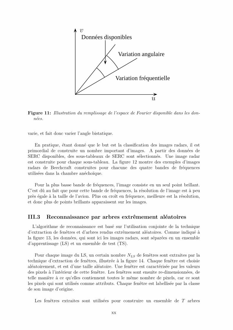
En illuminant l’objet sur une certaine bande de fréquences et à différents angles α,on remplit l’espace de Fourier. Bien entendu, étant donné que l’on est limité à unecertaine bande de fréquences et un certain espace angulaire, les valeurs de SERC nesont disponibles que pour une certaine portion de l’espace de Fourier, comme indiquéà la figure 11. L’image radar de l’objet illuminé est construite par application de latransformée de Fourier à deux dimensions aux valeurs de SERC.

b

Radar

b

x u

vy

α α

σ(f, θ)

⇐⇒2DFT

Espace de FourierEspace physique

Figure 10: Illustration de mesures de SERC en mode monostatique.

On généralise au cas bistatique en ajoutant à l’angle d’aspect le demi-angle bista-tique. L’image radar bistatique I(x, y) est alors obtenue à partir de la SERC

√σ(f, α)

par l’équation suivante:

I(x, y) =∫ +∞

0

∫ 2π

0

√σ(f, φ)e4πj f

ccos(β/2)(x cos(α+β/2)+y sin(α+β/2)|4f cos2(β/2)

c2|dβdf, (4)

où l’intégration est faite sur l’angle bistatique (et non pas sur l’angle d’aspect) car,dans la chambre anéchoïque, l’émetteur et l’objet sont fixes, tandis que le récepteur

xix

u

v

Variation angulaire

Variation fréquentielle

Données disponibles

Figure 11: Illustration du remplissage de l’espace de Fourier disponible dans les don-nées.

varie, et fait donc varier l’angle bistatique.

En pratique, étant donné que le but est la classification des images radars, il estprimordial de construite un nombre important d’images. A partir des données deSERC disponibles, des sous-tableaux de SERC sont sélectionnés. Une image radarest construite pour chaque sous-tableau. La figure 12 montre des exemples d’imagesradars de Beechcraft construites pour chacune des quatre bandes de fréquencesutilisées dans la chambre anéchoïque.

Pour la plus basse bande de fréquences, l’image consiste en un seul point brillant.C’est dû au fait que pour cette bande de fréquences, la résolution de l’image est à peuprès égale à la taille de l’avion. Plus on croît en fréquence, meilleure est la résolution,et donc plus de points brillants apparaissent sur les images.

III.3 Reconnaissance par arbres extrêmement aléatoires

L’algorithme de reconnaissance est basé sur l’utilisation conjointe de la techniqued’extraction de fenêtres et d’arbres rendus extrêmement aléatoires. Comme indiqué àla figure 13, les données, qui sont ici les images radars, sont séparées en un ensembled’apprentissage (LS) et un ensemble de test (TS).

Pour chaque image du LS, un certain nombre NLS de fenêtres sont extraites par latechnique d’extraction de fenêtres, illustrée à la figure 14. Chaque fenêtre est choisiealéatoirement, et est d’une taille aléatoire. Une fenêtre est caractérisée par les valeursdes pixels à l’intérieur de cette fenêtre. Les fenêtres sont ensuite re-dimensionnées, detelle manière à ce qu’elles contiennent toutes le même nombre de pixels, car ce sontles pixels qui sont utilisés comme attributs. Chaque fenêtre est labellisée par la classede son image d’origine.

Les fenêtres extraites sont utilisées pour construire un ensemble de T arbres

xx

Cross−range [Pixel]

Ran

ge [P

ixel

]

Sample Beech image reconstructed from its C−RCS’s [dB]

20 40 60 80 100 120 140 160 180 200

20

40

60

80

100

120

140

160

180

200 −20

−18

−16

−14

−12

−10

−8

−6

−4

−2

0

(a) Première bande de fréquences: [20; 80]MHz

Cross−range [Pixel]

Ran

ge [P

ixel

]

Sample Beech image reconstructed from its C−RCS’s [dB]

20 40 60 80 100 120 140 160 180 200

20

40

60

80

100

120

140

160

180

200 −20

−18

−16

−14

−12

−10

−8

−6

−4

−2

0

(b) Seconde bande de fréquences:

[190; 250] MHz

(c) Troisième bande de fréquences:

[450; 550] MHz

Cross−range [Pixel]

Ran

ge [P

ixel

]

Sample Beech image reconstructed from its C−RCS’s [dB]

20 40 60 80 100 120 140 160 180 200

20

40

60

80

100

120

140

160

180

200 −20

−18

−16

−14

−12

−10

−8

−6

−4

−2

0

(d) Quatrième bande de fréquences:

[1.2; 1.3] GHz

Figure 12: Exemple d’images radars de Beechcraft construites à partir de SERC, pourchacune des quatre bandes de fréquences utilisées.

xxi

Figure 13: Bloc-diagramme du classificateur.

Figure 14: Illustration de l’extraction de fenêtres sur une image. Les attributs sontles pixels de ces fenêtres préalablement mises à la même échelle, de sorte que chaquefenêtre contient le même nombre de pixels.

extrêmement aléatoires (extra-trees). La figure 15 illustre un arbre de décision. Unarbre de décision est un ensemble hiérarchique de nœuds reliés entre eux par desbranches. A chaque nœud, on teste un des attributs des fenêtres, l’un des pixelsdes fenêtres en l’occurrence. On sépare ensuite l’ensemble des fenêtres en deuxsous-ensembles, suivant le résultat du test. On continue à développer l’arbre jusqu’àce qu’un nœud ne contienne que des fenêtres appartenant toutes à la même classe.

La différence entre un arbre de décision classique et un extra-tree réside dansle choix du couple attribut-valeur seuil (ai, vi) pour chaque nœud. Dans un arbrede décision classique, le meilleur couple est choisi à chaque nœud. Pour un arbrealéatoire, le meilleur couple est choisi parmi un ensemble restreint de couples choisisaléatoirement.

La classe d’une image du TS est déterminée de la manière suivante: un nombreNTS de fenêtres sont extraites de l’image et ensuite re-dimensionnées. Chacune deces fenêtres est propagée dans chacun des T extra-trees du modèle de reconnaissance.

xxii

c1

c1c2

a1 < v1

a2 < v2

Yes No

Yes No

a1 < 5

a2 < 7

Figure 15: Illustration d’un arbre de décision.

La classe de l’image est déterminée par un vote de majorité sur les NTS × T classesobtenues par la propagation de chaque fenêtre dans chaque arbre.

III.4 Expériences de reconnaissance

L’algorithme de reconnaissance a été conçu pour être utilisé principalement sur desimages optiques. Il importe donc d’abord de le valider sur des images radars. Pour cefaire, nous le testons sur les images de la base de données MSTAR afin de comparer lesrésultats obtenus avec ceux obtenus par d’autres méthodes et publiés dans la litérature.Ensuite, l’algorithme est testé sur les images construites à partir des données de lachambre anéchoique de l’ONERA.

III.4.1 Reconnaissance sur les images MSTAR

La version de la base de données MSTAR utilisée se compose d’images de 5objets; les chars BMP-2 et BTR-70, le tank T-72, des fausses cibles, et d’imagesd’environnement, telles qu’illustrées à la figure 16. Chaque type d’objets est considérécomme une seule classe. Il y a donc cinq classes d’objets.

En appliquant l’algorithme de reconnaissance à la base de données MSTAR, onobtient des résultats de classification correcte de l’ordre de 98%, à condition de réduirele speckle présent dans les images autour des objets en eux-mêmes. Ce taux de recon-naissance est parmi les meilleurs résultats publiés dans la litérature. L’application del’algorithme de reconnaissance basé sur les extra-trees à des images radars est doncexpérimentalement validé.

III.4.2 Reconnaissance sur les images ONERA

Les données sont acquises en chambre anéchoïque pour 4 types d’avions (figure17) sur 4 bandes de fréquences (FB1 = [20; 80] MHz, FB2 = [190; 250] MHz, FB3= [450; 550] MHz et FB4 = [1.2; 1.3] GHz), sur 4 couples de polarisation émetteur-récepteur (HH , HV , V H et V V ), pour 3 angles d’aspect (α ∈ {0◦, 45◦, 90◦}), et pour

xxiii

(a) Char BMP-2. (b) Char BTR-70. (c) Tank T-72.

(d) Exemple d’image de

fausse cible.

(e) Exemple d’image

d’environnement.

(f) Exemple d’image

d’environnement.

Figure 16: Illustration des cinq classes des données MSTAR.

des angles bistatiques allant de 6◦ à 160◦. Les images sont construites en utilisant lesdonnées acquises pour la polarisation HH .

(a) Beechcraft. (b) F117.

(c) F16. (d) Learjet.

Figure 17: Modèle CAD de chacun des avions utilisés.

Les résultats obtenus donnent un taux de reconnaissance d’à peu près 30% pourles images de la FB1. Ce faible taux de reconnaissance s’explique par (1) la faiblerésolution des images qui est comparable à la taille des avions, et (2) par le fait quepour la FB1, la taille des avions influence plus la SERC que leur forme et que tousles avions sont de même taille. A l’inverse, les taux de reconnaissance sont proches de

xxiv

100% pour les trois hautes bandes de fréquences car la résolution des images est plusélevée et que la forme des avions influence plus la SERC que leur taille.

III.5 Conclusion

Dans cette section, nous avons procédé à la reconnaissance des avions en utilisantleurs images radars et un algorithme de reconnaissance basé sur l’utilisation d’arbresrendus extrêmement aléatoires. L’algorithme de reconnaissance a d’abord été testésur des images radars de la base de données MSTAR, et ensuite sur les images radarsconstruites à partir des SERC d’avions fournies par des mesures en chambre anéchoïque.Les taux de reconnaissance avoisinent les 100%, à l’exception de la bande de fréquencesdisponible la plus basse, étant donné que tous les avions sont de même taille et, à cettefréquence, n’apparaissent chacun que comme un seul point brillant.

IV Reconnaissance de cibles via leurs SER com-

plexes et réelles

IV.1 Introduction

La reconnaissance par imagerie, bien que très performante, nécessite la constructiond’images radars des cibles. Pour construire une image radar d’une cible, un utilisateurdoit disposer de valeurs de SERC sur une certaine partie de l’espace de Fourier. Ilfaut donc pouvoir disposer de paires émetteurs-récepteurs opérant sur des fréquencesadjacentes et dont les angles bistatiques soient également adjacents. En pratique,à cause des principes d’allocation des fréquences, il est invraisemblable de pouvoirdisposer d’émetteurs opérant sur des fréquences adjacentes et étant adjacents.

On cherche donc à reconnaitre les avions en utilisant directement leur SER, réelleou complexe, acquise à partir d’un nombre limité de paires émetteur-récepteur, commeindiqué à la figure 18. Par rapport au bloc-diagramme de la figure 9, l’étape de con-struction d’images radars a été supprimée.

IV.2 Reconnaissance par méthodes de sous-espaces

La figure 19 montre le bloc-diagramme de l’étage de reconnaissance de la figure 18.L’algorithme de reconnaissance est basé sur les méthodes de sous-espaces.

Les données, soit de SER, soit de SERC, sont séparées en un ensembled’apprentissage (LS) et un ensemble de test (TS). Des vecteurs d’attributs sontformés pour chaque classe représentée dans le LS. Chaque vecteur d’attributs consisteen une séquence de valeurs de SER ou de SERC acquises à des angles bistatiquesconsécutifs. Chaque vecteur d’attributs peut donc être vu comme la réalisation d’unevariable aléatoire représentant la SER ou la SERC pour ces angles bistatiques. Pourchaque classe, l’ensemble des vecteurs d’attributs est concaténé dans une matrice,notée X.

Chaque classe est caractérisée par un sous-espace construit par décompositionen valeurs singulières de la matrice X. On a donc X : UΣV H , où U est la matrice

xxv

Figure 18: Bloc-diagramme du système de reconnaissance automatique de cibles basésur les SER complexes (SERC) ou réelles (SER) des avions.

des vecteurs singuliers, et Σ la matrice diagonale des valeurs singulières. Le meilleursous-espace est constitué en gardant les vecteurs singuliers de U correspondant auxvaleurs singulières de Σ les plus grandes. Le modèle de reconnaissance consiste doncen un ensemble de sous-espaces, chaque sous-espace représentant une classe.

La classe d’un vecteur d’attributs du TS est déterminée de la manière suivante. Levecteur est projeté dans chacun des sous-espaces du modèle de reconnaissance. Ensuite,une mesure de chaque projection, équivalente à l’énergie de la projection du vecteurdans chacun des sous-espaces, est calculée. La classe attribuée à ce vecteur est cellecorrespondant au sous-espace dont l’énergie de la projection est la plus grande.

IV.3 Expériences de reconnaissance sur les données ONERA

Le modèle de reconnaissance automatique de cibles décrit plus haut est testé suc-cessivement sur les SER puis sur les SERC des quatre avions présentés précédemment.Rappelons que les valeurs de SER et de SERC sont acquises en chambre anéchoïque.Le cas d’une seule paire émetteur-récepteur est d’abord testé. Les taux de recon-naissance sont indiqués à la figure 20 par bande de fréquences, pour la polarisation HH .

Pour la bande de fréquences la plus faible, les taux de reconnaissance sont trèsfaibles, alors qu’ils augmentent aux fréquences plus élevées, et ce pour les mêmesraisons que dans le cas des images radars. Pour chaque bande de fréquences, le tauxde reconnaissance varie suivant la région de l’espace (α, β) dans laquelle l’objet estilluminé.

On voit aussi clairement qu’il est plus intéressant de travailler avec la SERcomplexe (donc la phase) que réelle. C’est probablement dû à la différence dans lesformes des avions utilisés.

Le cas de trois paires émetteur-récepteur est ensuite considéré. La classe d’unavion est déterminée par vote de majorité sur les résultats de classification de chaque

xxvi

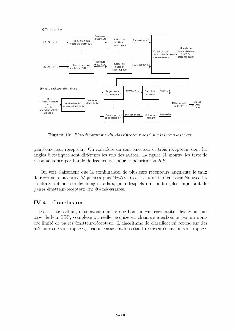
Figure 19: Bloc-diagramme du classificateur basé sur les sous-espaces.

paire émetteur-récepteur. On considère un seul émetteur et trois récepteurs dont lesangles bistatiques sont différents les uns des autres. La figure 21 montre les taux dereconnaissance par bande de fréquences, pour la polarisation HH .

On voit clairement que la combinaison de plusieurs récepteurs augmente le tauxde reconnaissance aux fréquences plus élevées. Ceci est à mettre en parallèle avec lesrésultats obtenus sur les images radars, pour lesquels un nombre plus important depaires émetteur-récepteur ont été nécessaires.

IV.4 Conclusion

Dans cette section, nous avons montré que l’on pouvait reconnaitre des avions surbase de leur SER, complexe ou réelle, acquise en chambre anéchoïque par un nom-bre limité de paires émetteur-récepteur. L’algorithme de classification repose sur desméthodes de sous-espaces, chaque classe d’avions étant représentée par un sous-espace.

xxvii

0 FB1 FB2 FB3 FB40

0.2

0.4

0.6

0.8

1

Bande de fréquence

Pcc

SERC

SER

Figure 20: Taux de reconnaissance moyen par bande de fréquences, pour une seulepaire Tx-Rx. La variation au sein d’une même bande dépend de la région du plan(α, β) dans laquelle l’objet est illuminé.

FB1 FB2 FB3 FB40

0.1

0.2

0.3

0.4

0.5

0.6

0.7

0.8

0.9

1

Bande de fréquence

Pcc

SERC

SER

Figure 21: Taux de reconnaissance moyen par bande de fréquences, pour trois pairesTx-Rx. La variation au sein d’une même bande dépend de la région du plan (α, β)dans laquelle l’objet est illuminé.

xxviii

V Reconnaissance de cibles via leurs SER réelles,

acquises expérimentalement

V.1 Introduction

Dans la section précédente, on a montré que l’on pouvait reconnaitre de manièreperformante des avions en utilisant leur SER, complexe ou réelle, acquise en chambreanéchoïque. On teste maintenant la reconnaissance d’avion en utilisant leur SERréelle acquise à partir d’un banc de test basé sur un radar passif bistatique, déployéen extérieur.

Les opérations à mener ont été décrites à la figure 1. Les avions doivent d’abordêtre détectés et localisés. Un émetteur d’opportunité est sélectionné afin d’acquérir sonsignal qui est réfléchi par les avions détectés. La SER des avions est extraite de ce signalacquis, et sert ensuite à leur reconnaissance. La figure 22 représente le bloc-diagrammede ce système de reconnaissance.

Figure 22: Bloc-diagramme du système de reconnaissance automatique de cibles basésur les SER des avions acquises par banc de test expérimental.

V.2 Banc de test de radar passif bistatique

Le banc de test déployé aux alentours de l’aéroport d’Orly (figure 23) consiste en unrécepteur ADS-B et un récepteur SDR basé sur la radio-logicielle. Les signaux ADS-Bservent à la détection et à la localisation des avions, étant donné que les signauxADS-B émis par les avions commerciaux contiennent leurs informations de localisation.

Le récepteur ADS-B a permis de détecter 1329 avions pendant une campagneayant duré une dizaine de jours. Parmi ces avions, les 47 Airbus de la famille des A340(65 mètres de long, 4 moteurs) sont utilisés comme classe de grands avions, et les 549Airbus de la famille des A320 (35 mètres de long, 2 moteurs) comme classe d’avionsde taille moyenne.

L’émetteur d’opportunité sélectionné est un VOR (celui de Rambouillet) ser-vant à la navigation aérienne. Plus précisément, une sous-porteuse de son signalest utilisée comme signal d’opportunité. Le récepteur SDR permet d’acquérir à

xxix

Figure 23: Configuration du banc de test déployé. L’émetteur sélectionné est le VORde Rambouillet. Les récepteurs sont localisés au point marqué "HOUSE". Le cercleindique la région dans laquelle les avions sont détectés, de par le rapport signal-sur-bruit suffisamment élevé des signaux réfléchis par les avions.

la fois le signal émis par le VOR qui est reçu directement, et le signal réfléchipar un avion, comme le montre l’exemple de spectrogramme des signaux reçus àla figure 24. Ces deux signaux sont utilisés pour le calcul de la SER des avions détectés.

La SER des avions est calculée de la manière suivante. La puissance du signal direct,notée PRD, et la puissance du signal réfléchi, notée PRS, correspondent, à chaque instantt, aux pics du signal direct et du signal réfléchi sur le spectrogramme de la figure 24.En combinant l’équation radar bistatique et l’équation de bilan de liaison, la SER peuts’exprimer comme

σ =PRSPRD

GRT

GRSG

(4π)3R2TSR

2RS

λ2L, (5)

où les différentes grandeurs sont indiquées sur la figure 25. La figure 26 montre lesvaleurs de SER des avions de taille moyenne en fonction des angles d’aspect α etbistatique β. Il est clair que les valeurs sont cohérentes d’un avion à l’autre, et qu’ellespeuvent donc être utilisées pour reconnaitre les avions.

Afin d’ajouter une classe d’avions, la SER d’avions de petite taille (4 mètres delong) est simulée de manière numérique en utilisant les trajectoires des avions de taillemoyenne. Ce type d’avions n’étant pas équipé d’émetteur ADS-B, le banc de test nepermet pas de les détecter, d’où le recours à la simulation.

La base de données consiste donc en des valeurs de SER de trois classesd’avions. Pour chaque classe d’avions, un tiers des avions détectés forme l’ensembled’apprentissage, et les deux autres tiers forment l’ensemble de test.

V.3 Reconnaissance par méthodes de sous-espaces

Le même algorithme de classification basé sur les méthodes de sous-espaces et décritprécédemment est utilisé pour procéder à la reconnaissance des avions. La figure 27montre le taux de reconnaissance obtenu par région de l’espace (α, β). Les régions enbleu correspondent à des zones pour lesquelles aucune donnée n’a pu être récoltée. Letaux de reconnaissance obtenus pour les autres régions varie de 40% à 99%. Le taux

xxx

Signal direct Signal réfléchi par l’avion

Figure 24: Exemple de spectrogramme d’un signal reçu. On distingue le signal directpar sa fréquence fixe, et le signal réfléchi par un avion présentant un shift Doppler.

global de reconnaissance obtenu est de 83%.

Certaines régions apparaissent donc plus intéressantes que d’autres pour la recon-naissance des classes d’avions décrites ci-dessus. Étant donné que les couloirs aérienssont déterministes, il convient alors de bien choisir l’emplacement du récepteur pourobtenir un taux de reconnaissance élevé.

V.4 Conclusion

Dans cette section, on a montré que des avions commerciaux peuvent être reconnusde manière performante sur base de leur SER réelle acquise à partir d’un banc detest déployé aux alentours de l’aéroport d’Orly et basé sur un radar passif bistatiqueutilisant un VOR comme émetteur d’opportunité et un récepteur de radio-logicielle.

xxxi

GTRT

R

S

RTS RRS

RTR PRD

PRS

(Avion)

(Tx)

(Rx)b

b GTS

L

b

bGRS

GRT

bbb

b

b

β

Figure 25: Configuration radar bistatique correspondant à une paire Tx-Rx et unavion. T , R, and S indiquent les positions du Tx, du Rx, et de l’avion, respective-ment. Le graphe montre les diagrammes de rayonnement des antennes d’émissionet de réception. Les différents paramtres de l’équation (5) y sont indiqués.

0 50 100 150 200 250 300 3500

20

40

60

80

100

120

140

160

180

α [°]

β [°

]

RCS [dBsm]

10

20

30

40

50

60

70

Figure 26: Valeurs de SER pour les avions de taille moyennes, dans le plan (α, β).

xxxii

Figure 27: Taux de reconnaissance des avion par région de l’espace (α, β).

VI Conclusions et perspectives

Dans cette thèse, nous avons étudié la problématique de la reconnaissance d’avions(aussi appelés cibles) en utilisant des signaux de radars passifs bistatiques, en vuede la détection d’anomalies dans le trafic aérien civil. Une anomalie peut en effetsurvenir quand un avion n’est pas équipé pour répondre aux interrogations de radarssecondaires.

Une stratégie de reconnaissance a d’abort été définie, basée sur la phénoménologieradar. En effet, la SER, complexe ou réelle, d’un objet dépend de quatre facteursque sont la fréquence du signal transmis, le couple de polarisation de l’émetteur etdu récepteur, l’angle d’aspect et l’angle bistatique. Etant donné que les mécanismesde diffusion contribuant à la SER dépendent de ces quatre paramètres et qu’il estpar ailleurs invraisemblable d’observer un avion sur l’entièreté de sa trajectoire, lastratégie de reconnaissance consiste en la séparation de cet espace de paramètres enrégions, et en la construction d’un classificateur par région.

Les premières expériences de reconnaissance ont été menées sur des donnéesacquises en chambre anéchoïque. Les avions ont d’abord été reconnus en utilisant leursimages radars construites à partir des SER complexes, et en appliquant l’algorithmedes arbres rendus extrêmement aléatoires sur ces images radars. Bien qu’ayant obtenusdes taux de reconnaissance excellents, la construction d’images demande l’utilisationd’un certain nombre de paires émetteur-récepteur. Les avions ont donc été reconnusen utilisant directement leur SER, réelle ou complexe, et en utilisant un classificateurbasé sur les méthodes de sous-espaces. Les taux de reconnaissance obtenus varientsuivant la région de l’espace des paramètres dans laquelle est illuminé l’avion, etpeuvent atteindre 98%.

Afin de tester l’algorithme de reconnaissance sur des données de SER réelles, un

xxxiii

banc de test basé sur un radar passif bistatique a été dployé aux alentours de l’aéroportd’Orly. Le banc de test détecte et localise les avions en utilisant leurs signaux ADS-B.Le signal d’opportunité choisi est la sous-porteuse du signal émis par un VOR. LaSER des avions est calculée sur base du ratio entre la puissance du signal réfléchisur les avions et la puissance du signal direct, ces signaux étant collectés par unrécepteur de radio-logicielle. L’algorithme de reconnaissance est basé sur les méthodesde sous-espaces. Le taux de reconnaissance obtenu est de 83% et varie suivant lesrégions de l’espace des paramètres, démontrant ainsi expérimentalement la faisabil-ité de la reconnaissance de cibles par utilisation de signaux de radars passifs bistatiques.

Différentes perspectives sont envisagées afin de rendre le système le plus opéra-tionnel possible. Tout d’abord, il convient de pouvoir détecter et localiser les ciblesd’une autre manière qu’en utilisant les signaux ADS-B, par définition des anomaliesdans le trafic aérien. Ensuite, différents émetteurs d’opportunité peuvent être utiliséset combinés, la bonne localisation des récepteurs et des émetteurs pouvant permettred’augmenter significativement le taux de reconnaissance. L’utilisation de la phase dela SER peut aussi contribuer à améliorer les résultats de reconnaissance. Étant donnéque les taux de reconnaissance varient suivant la polarisation, l’angle d’aspect et l’anglebistatique, il conviendrait d’étudier théoriquement l’influence de ces paramètres. En-fin, nous donnons quelques pistes concernant la reconnaissance elle-même, telles quel’utilisation d’autres techniques de classification, ou la définition des classes de ciblessuivant des méthodes d’apprentissage non-supervisé comme le clustering.

xxxiv

Chapter 1

Introduction

Contents1.1 Motivation for the thesis . . . . . . . . . . . . . . . . . . . . 1

1.1.1 Targets considered . . . . . . . . . . . . . . . . . . . . . . . . 2

1.1.2 Automatic target recognition (ATR) . . . . . . . . . . . . . . 2

1.1.3 Class of a target . . . . . . . . . . . . . . . . . . . . . . . . . 3

1.1.4 Bistatic radar . . . . . . . . . . . . . . . . . . . . . . . . . . . 3

1.1.5 Passive radar . . . . . . . . . . . . . . . . . . . . . . . . . . . 3

1.2 Developed techniques . . . . . . . . . . . . . . . . . . . . . . 5

1.2.1 Scene parameters . . . . . . . . . . . . . . . . . . . . . . . . . 5

1.2.2 Quantities used for the recognition of targets . . . . . . . . . 6

1.2.3 Proposed ATR systems . . . . . . . . . . . . . . . . . . . . . 6

1.3 Background: conventional air traffic control (ATC) . . . . 8

1.3.1 Primary surveillance radar . . . . . . . . . . . . . . . . . . . 9

1.3.2 Secondary surveillance radar . . . . . . . . . . . . . . . . . . 10

1.3.3 Non-cooperative target recognition within ATC . . . . . . . . 11

1.4 Contributions of the thesis . . . . . . . . . . . . . . . . . . . 11

1.5 Organization of the manuscript . . . . . . . . . . . . . . . . 12

1.6 Conclusion . . . . . . . . . . . . . . . . . . . . . . . . . . . . 13

1.1 Motivation for the thesis

The motivation for this thesis is the automatic recognition of targets using passivebistatic radar signals. The objective of the thesis is to design, implement, and testa system able to recognize, at low cost, targets. We call this system an automatictarget recognition (ATR) system. In this section, we define the types of targets thatare considered, and the notions of ATR, target class, bistatic radar, and passive radar.

1

2 1.1. MOTIVATION FOR THE THESIS

1.1.1 Targets considered

In this work, we consider non-cooperative targets. Non-cooperative targets aretargets that do not provide information about their identity or location when asked todo so, by contrast with cooperative targets that provide this information. Examplesof non-cooperative targets are personal cars. In general, we often refer to targets asobjects.

Without loss of generality, we consider non-cooperative air targets. Non-cooperativeair targets are not able to reply to requests from air traffic control (ATC) radars,either because of the absence of a transponder on-board, because of a failure of sucha transponder, or because the transponder is off (willingly or not). ATC is describedin Section 1.3. We discuss the application of the proposed ATR systems, described inSection 1.2, to other types of targets in Chapter 9.

1.1.2 Automatic target recognition (ATR)

Automatic target recognition (ATR) is defined as the process of recognizing targetswithout human involvement [17, 95, 173]. ATR is called non-cooperative target recog-nition (NCTR) in case of non-cooperative targets, as in this thesis, and identificationfriend-or-foe (IFF) in case of cooperative targets [187]. NCTR aims at recognizinga target from the radar echo signals received from the target to be recognized. IFFsystems rely on the interrogation of the transponder on-board the target that sendsits identification back to the interrogator.

The word "recognition" in ATR implies classification. We equivalently use bothterms in this thesis. Classification is defined as the act of assigning to input data oneclass among a set of pre-defined classes [54,134]. The task of the classifier is to assign aclass to an unknown object described by features, called attributes. To do so, the clas-sifier derives rules from objects described by attributes and for which their respectiveclass is known. Usually, a classification model describing these rules is derived usinga subset of the available data called the learning set (LS). The classification model istested on another subset of the data called the test set (TS). Other ways of partitioningthe data, such as cross-validation, can be used [134]. Cross-validation is used when theamount of data is insufficient to create an LS and a TS that are independent, and thateach contains a sufficient amount of objects. We do not consider cross-validation inthis thesis since a particular effort is made to obtain a dataset as complete as possible.The fact that we learn and train the ATR systems, described in Section 1.2, on realdata, making up complete datasets, is another key feature of this thesis. Indeed, as willbe explained in Chapter 2, many ATR systems for passive radar rely on simulated data.

Classification is a part of supervised learning [54, 134]. In supervised learningproblems, objects belong to different categories, called classes. Supervised learningaims at deriving relationships between the attributes of objects. These relationshipsare used to predict the true class of an object. Supervised learning problems are eitherregression problems or classification problems. In regression problems, the predictionis a (continuous) numerical value, whereas in classification problems the predictedoutput is a discrete class.

1.1. MOTIVATION FOR THE THESIS 3

Supervised learning is a part of machine learning. Machine learning is a subfield ofautomatic learning that aims at designing rules that are similar to those that humanexperts derive [221]. In machine learning problems, each object is characterized by aset of features called attributes. Machine learning is divided into supervised learningand unsupervised learning. Unsupervised learning, also called clustering, aims atderiving probabilistic or causal relationships between objects. For example, clusteringmethods try to form groups of objects based on the features of the objects. The use ofunsupervised learning in our ATR problem is part of our future work, and is discussedin Chapter 9.

In short, the problem addressed in this thesis is an ATR problem, and more specif-ically, an NCTR problem. We aim at classifying/recognizing non-cooperative air tar-gets. Air targets are characterized by some number of attributes.

1.1.3 Class of a target

In this work, the proposed ATR systems label each unknown target of interest witha particular target class. The notion of target class is not uniquely defined in theradar ATR literature. The nature of the prediction of a classifier thus varies from oneATR system to the other. For example, a target is defined in [187] first accordingto its general nature, which can be defined as aircraft, ship, or bird. Each type ofgeneral nature of target is then divided into different target types. Example targettypes for airplanes are fighter planes and helicopters. Each target type can be furtherseparated into different target classes that can be F16, F22, and B2. The callsign of atarget, such as AF123, can eventually be determined. This latter operation is referredto as identification, and not as classification/recognition. Identification is usuallyimplemented in a cooperative target recognition system (IFF), since it requires thetarget to send its identification number or identification code.

In this thesis, we use a single target class for all airplanes sharing the same physicalproperties. Looking ahead to Chapter 8, large-size airplanes and mid-size airplanesshall be labelled two different classes, while an A318 airplane and an A319 airplaneshall be labelled the same class, since they are both mid-size airplanes.

1.1.4 Bistatic radar

A radar system is called bistatic (BS) when the transmitter and the receiver arenot co-located, as shown in Fig. 1.1, by contrast with the monostatic (MS) radar forwhich the transmitter and the receiver are co-located [89]. By comparison with MSconfigurations, a BS configuration is characterized by an additional parameter, whichis the bistatic angle, β. The bistatic angle β is defined as the angle (defined to bepositive and less than 180◦) between the transmitter and the receiver, with its vertexat the target [224].

1.1.5 Passive radar

Passive radars are radars that use illuminators of opportunity as transmitters. Illu-minators of opportunity are transmitters that are already present in the environment,

4 1.1. MOTIVATION FOR THE THESIS

Target

BaselineTransmitter Receiver

Transmission path Echo pathβ

Figure 1.1: Bistatic geometry for one pair of transmitter and receiver.

such as analog TV transmitters, digital video broadcast - terrestrial (DVB-T) TVtransmitters, or mobile phone base transceiver stations (BTSs). We propose to useone or multiple illuminators of opportunity as source of radar illumination, as in [225].It is assumed that the different characteristics of the signals transmitted illuminatorsof opportunity, such as their location, frequency, modulation, and polarization areknown but are not controlled.

The qualifier "passive" means that the transmitter is not aware of being used as aradar transmitter, although it must evidently be active. The transmitter is thus callednon-cooperative. The different illuminators of opportunity that are used in actualpassive radar systems are presented in Chapter 2.

Since the transmitter used is already present, the implementation of a passive radarrequires few technical investments, especially since fast digital signal processors thatmake the acquisition and the processing of the scattered signals easy are available.Using illuminators of opportunity thus contributes to the low-cost aspect of thesolution. Another advantage of a passive radar is that, since the transmitter is alreadyoperational, it allows for an immediate access to the frequency spectrum. The maindisadvantage is that the characteristics of the signal transmitted are not controlled,since such a transmitter is usually not designed specifically for radar purposes.

Illuminators of opportunity considered in this work operate on the "low" frequencybands, defined here as frequencies lower than 1 GHz. The use of low frequenciesfor classification/recognition purposes is justified by the following reasons. First,since the wavelength is of the order of several meters, and since the length of thetargets are of the order of tens of meters, the radar signature and its variations areessentially dependent on the larger parts of a target, and less sensitive to its smallerparts. The signature is thus robust and reproducible from one aircraft to the otherat low frequencies. Second, transmitters operating at low frequencies are presenteverywhere in the environment: radio transmitters, TV transmitters, mobile phoneBTSs. Therefore, the use of signals transmitted at these corresponding frequencies isstraightforward. Third, low frequencies are suitable to defeat the possible stealthinessof air targets. Indeed, at low frequencies, no material can efficiently absorb theenergy of the incident wave and be used in operation. Absorbing energy at these low

1.2. DEVELOPED TECHNIQUES 5

frequencies would require that the size of the stealth layer be very large, of the orderof the wavelength, i.e. of about 3 m for a signal transmitted at a frequency of 100 MHz.

Passive radars are inherently bistatic. Such radars are called passive bistatic radars(PBRs). As explained in Chapter 2, PBRs are mainly used today for detection andlocation purposes. The use of PBRs for the recognition of air targets is a key featureof this thesis.

1.2 Developed techniques

We use radar signals transmitted by one or multiple transmitters (Tx’s) of oppor-tunity, scattered by a target, and collected by one or multiple receivers (Rx’s). Theconfiguration of the radar system is shown in Fig. 1.2 for a single (Tx,Rx) pair. Thethree ATR systems implemented in this thesis assign a class to the unknown, detectedair target from the signal scattered by this air target and from the direct signal. Theperformances of the three proposed ATR systems will be compared in Chapter 9, interms of (1) their probabilities of correct recognition, defined as the ratio of the numberof objects correctly recognized to the total number of objects, and (2) the number of(Tx,Rx) pairs needed.

Figure 1.2: Configuration of the radar system for a single (Tx,Rx) pair. An ATRsystem assigns a class to the unknown, detected air target based on the receivedscattered signal.

1.2.1 Scene parameters

We assume that an unknown airplane to recognize has already been detected andtracked: we know its position and line-of-sight, i.e. its direction. However, we do notknow its exact orientation, i.e. its yaw, pitch, and roll angles. These assumptions arerealistic since the detection and tracking of an airplane is performed by a primary

6 1.2. DEVELOPED TECHNIQUES

surveillance radar (PSR) when the airplane is taking-off or landing, as described inSection 1.3. When the airplane is en-route, passive bistatic radars (PBRs) can detectand track airplanes, as explained in Chapter 2.

We assume that we know the location, polarization, and frequency of the Tx(s)of opportunity used, but we do not control them. We also assume that we know thelocation and polarization of the Rx(s), since the Rx(s) are under our full control. Wecall these parameters the scene parameters.

1.2.2 Quantities used for the recognition of targets

Consider the case of a PBR consisting of a single Tx of opportunity and a single Rx.One can extract, from the signal transmitted by the Tx, scattered by the unknown,detected air target, and collected by the Rx, the bistatic complex radar cross-section(BS-CRCS) and the bistatic radar cross-section (BS-RCS), which both characterizethe target. We present the notions of BS-CRCS and BS-RCS in Chapter 3. Theextraction of both the BS-CRCS and the BS-RCS from the signal scattered by an(air) target is explained in Chapter 4.

As described in Chapter 2, images of targets are often used in ATR. The radarimage of a target is defined as a two-dimensional (2D) BS-CRCS density. We thusfirst perform the recognition of targets by using their radar images constructed fromtheir BS-CRCS.

However, constructing radar images of air targets based on signals transmitted byilluminators of opportunity is difficult, as the required space and frequency diversityconstraints (described in Chapter 5) would be difficult to meet in an operationalsystem. Therefore, in a second step, we suggest to recognize targets by using eithertheir BS-CRCS or their BS-RCS.

We test the first two ATR systems on data acquired in an anechoic chamber. Forthe third ATR system, we recognize targets by using their real-life BS-RCS, since, asshown in Chapter 8, the phase of the BS-CRCS is difficult to acquire in an operational,outdoor ATR system.

1.2.3 Proposed automatic target recognition (ATR) systems

We present three ATR systems. The three systems share the following characteristics:

• The raw input data of each ATR system consists of the signals transmitted byan illuminator of opportunity, scattered by a detected air target, and collectedby a receiver. The input data is separated into a learning set (LS), and a test set(TS).

• The scene parameters are known, and are an input of each of the three ATRsystems.

• The recognition, that we also call the classification, consists in a learning stepand a test step. The learning step consists in the construction of the target class

1.2. DEVELOPED TECHNIQUES 7

model based on data in the LS. The test step consists in the determination ofthe target class of data in the TS, thus attributing a class to each data instanceof the TS.

• The output of each of the three ATR systems is the class of the unknown, detectedair target. We quantify the performance of each of the three ATR systems bycomputing the probability of correct recognition for each.

The three following subsections give a block diagram of each of our three ATRsystems, as well as the characteristics of each of them.

ATR system using radar images

Our first ATR system recognizes targets by using their radar images. We will usethis system as a reference to evaluate our two other ATR systems, which recognizetargets by using either their BS-CRCS or their BS-RCS.

Figure 1.3 shows the block diagram of this first ATR system. The BS-CRCS of thetargets are extracted from the raw input data, for both the LS and the TS (Chapter 4).The images of targets are then constructed from these BS-CRCS (Chapter 5). Theimages in the LS are used to generate the target class model. The target class of eachimage of the TS is determined by passing each image in the TS through the targetclass model (Chapter 6).

Figure 1.3: Block diagram of our ATR system using radar images of targets.

ATR system using either bistatic complex RCS (BS-CRCS) or bistatic RCS(BS-RCS)

Since the construction of images of targets is not feasible in an operational low-frequency passive bistatic radar system, as will be described in Chapter 5, we recognizetargets by directly using either their BS-CRCS or their BS-RCS. Figure 1.4 shows theblock diagram of our second ATR system. The BS-CRCS or the BS-RCS of the targetsare extracted from the raw input data, for both the LS and the TS (Chapter 4).The class of unknown targets is determined by passing either their BS-CRCS or theirBS-RCS through the target class model (Chapter 7).

8 1.3. BACKGROUND: CONVENTIONAL AIR TRAFFIC CONTROL (ATC)

Figure 1.4: Block diagram of our ATR system using the bistatic complex radar cross-sections or the bistatic radar cross-sections of targets.

ATR system using real-life bistatic radar cross-sections (BS-RCSs)

In order to design an operational ATR system, we add a detection stage anda discrimination and pre-classification stage to the second ATR system, as shownin Fig. 1.5. This ATR system, that we discuss in Chapter 8, will be tested in anoperational mode. For reasons to be explained in Chapter 8, we use the BS-RCS andnot the BS-CRCS of air targets.

Figure 1.5: Block diagram of our ATR system using real-life bistatic radar cross-sections of targets.

We perform the discrimination between detected targets of interest and other de-tected man-made targets in the discrimination and pre-recognition stage. The BS-RCSof the targets of interest are extracted in the extraction of BS-RCS stage, and are theinput of the recognition stage. The class of targets of interest is determined by passingtheir BS-RCS through the target class model.

1.3 Background: conventional air traffic control

(ATC)

In this thesis, we address the problem of the recognition of non-cooperative targets,called non-cooperative target recognition (NCTR). Since the targets considered inthis work are air targets, we describe the principles of air traffic control (ATC).

1.3. BACKGROUND: CONVENTIONAL AIR TRAFFIC CONTROL (ATC) 9

In Europe, ATC is performed by secondary surveillance radars (SSRs) when air-planes are en-route. Around airports, i.e. for take-off and landing operations, ATCis performed by airport surveillance radars (ASRs), consisting in the joint use of pri-mary surveillance radars (PSRs) and SSRs. In the United States, ASRs are used bothen-route and near airports [204]. We now briefly describe PSRs and SSRs, in order topoint out their limitations for ATC for the recognition of non-cooperative airplanes.

1.3.1 Primary surveillance radar

A primary surveillance radar (PSR), also called moving target detector (MTD), isa particular type of moving target indicator (MTI) radar [187, 204]. As for any radar,it sends out electromagnetic pulses. If an (air) target is present, the surface of thistarget will reflect the incident pulse back to the radar. The time taken by the pulse toreach the target and return to the PSR gives the distance from the radar antenna tothe target according to

D =cτ

2, (1.1)

where D is the distance from the antenna to the target, c the speed of light, and τ theround-trip delay.

The bearing of the target is given by the azimuth orientation of the PSR antenna.The elevation angle of the target is not measured. The PSR radar scans the entirehorizon at some scan rate, which means that a particular portion of the sky is notcontinuously monitored, therefore limiting the dwell time.

Figure 1.6 shows the key stages of a PSR radar [137]. First, the signal scatteredon the target is digitized by an analog-to-digital converter (ADC). Second, the signalscattered on the target is separated from clutter by using clutter cancellation filters,such as digital Doppler filters. Then, the signal scattered on the target is separatedfrom thermal noise using a constant false alarm rate (CFAR) thresholding algorithm.A scan-to-scan correlation-and-tracking algorithm generates a single report per target,from a cluster of range-azimuth-Doppler target reports, so that a target is representedby a single dot on the plan-position indicator (PPI).

Figure 1.6: Simplified block diagram of a primary surveillance radar.

The main advantage of the PSR is that it does not require the cooperation of thetarget itself. It is also capable of detecting small energy responses, making it availableto monitor weather. The main disadvantage of the PSR is its inability to discriminate

10 1.3. BACKGROUND: CONVENTIONAL AIR TRAFFIC CONTROL (ATC)

between targets presenting the same level of return energy. Another disadvantage ofthe PSR is the large amount of transmitting power required so that the echo signal hasa power high enough to be measurable. This limits its range. Moreover, echo signalsare subject to external factors such as changes of target attitude, resulting in fading ofthese echo signals.

1.3.2 Secondary surveillance radar

A secondary surveillance radar (SSR) is used to identify an air target, whetherit has been detected by a PSR radar [192] if the air target is near airports, ornot if it is en-route. SSRs can be seen as the civilian adaptation of the militaryidentification friend-or-foe (IFF) radar systems that were initially developed duringWorld War II [68]. During this war, air targets equipped with IFF systems had torespond with a specific signal to signals transmitted by ground-based transmitters. Acorrect response made the aircraft be identified as friend, while an incorrect responsemade the aircraft be identified as foe.

Figure 1.7 shows the principle of an SSR. The SSR transmitter sends out an inter-rogation signal to the transponder (transmitter/receiver working on radar frequencies)carried aboard the cooperative target. The on-board transponder responds to the SSRinterrogation by sending a signal containing information such as the target identity(squawk code) and position. Upon reception, the response signal is processed by thereceiver in order to identify the target on the operator plan-position indicator (PPI).If the target transponder does not respond, it is considered as a non-cooperative targetin civilian aviation, and as an enemy in military aviation.

Figure 1.7: Simplified block diagram of the receiving stage of a secondary surveillanceradar.

The main advantage of the SSR is that the transmitting power from the SSRtransmitter can be reduced. Indeed the power of the received signal decreases bya factor of D2 instead of D4 in the PSR case, since both the radar and the targettransmit in the SSR case. Another advantage is the complete identification andlocation of the air target through the information sent from the target.

1.4. CONTRIBUTIONS OF THE THESIS 11

The automatic dependent surveillance (ADS) system is the SSR used today. AnADS system relies on a transponder aboard an air target that transmits data, such as itsposition, altitude, and speed, to the ground station. Today, the automatic dependentsurveillance- broadcast (ADS-B) mode [22,209], which is part of the new Traffic Alertand Collision Avoidance System (TCAS), is used [9].

1.3.3 Non-cooperative target recognition (NCTR) within air

traffic control (ATC)

As described above, the identification process is based on the presence of atransponder aboard the air target, and on the confidence in the response from suchtransponder. In case there is no transponder aboard the target, or its transponder isnot working properly, or it is turned off, the target cannot be identified.

Near airports, one could think of analyzing the signals transmitted by the PSRand scattered by the air target back to the PSR to characterize the target. However,for conventional and existing PSRs, as the scan rate is high, the dwell time is limited,of the order of a few milliseconds. Moreover, as the range is important, the distanceresolution is also low. It is therefore difficult to analyze the target using a PSR, andeven more difficult to create an image or a high-resolution range profile of the targetto recognize it. Furthermore, because of the limited "time-on-target", PSRs will notbe used as transmitters of opportunity.

However, studies aiming at designing new PSRs that would be able to combineboth tracking and identification modes within the same scan are currently on-going.These new PSRs are not considered here, as they are not operational yet.

In conclusion, the use of conventional PSRs and SSRs does not allow one to identifynon-cooperative targets. Moreover, even though SSRs are able to identify cooperativetargets, SSRs do not provide any verification mean, since SSRs trust the informationreceived from the target transponder.

1.4 Contributions of the thesis

We list here the main contributions of the thesis. First, we use low-frequencypassive bistatic radar signals for the classification/recognition of air targets. Indeed,many passive bistatic radar signals are used for the detection and location of targets,but not for their recognition. The use of illuminators of opportunity contributes tothe low-cost aspect of the proposed solution. The use of low-frequency radar signalsfor the recognition of targets is not common, since many automatic target recognition(ATR) systems operate at higher frequencies.

Our first ATR system recognize targets by using their radar images. Although theexpression for the construction of the radar image of a target from its bistatic complexradar cross-section (BS-CRCS) is known, we provide its derivation from the principlesof tomographic imaging, as second contribution. The reason is that we could not findthis derivation in the literature.

12 1.5. ORGANIZATION OF THE MANUSCRIPT

Third, we recognize non-cooperative air targets, based on either their BS-CRCS ortheir bistatic radar cross-section (BS-RCS). This is a major difference with many ATRsystems that mainly use either high-resolution range profiles or radar images of targets.

Fourth, we developed three ATR systems that use two recognition techniques,which are the extremely randomized trees and the subspace methods. To the best ofour knowledge, the use of tree-based classification methods in the radar ATR domainis novel. To the best of our knowledge, vector subspaces are mainly used in the radardomain for detection, and not for classification/recognition.

Fifth, we learn and train the recognition stage of each of our three ATR systemson real data.

Sixth, we deploy a passive bistatic radar that we use for the acquisition of real-lifepassive bistatic radar signals. We extract the real-life BS-RCS of commercial airplanesfrom these signals.

1.5 Organization of the manuscript

Chapter 2 presents a literature review of passive bistatic radars, illuminators ofopportunity, and automatic target recognition (ATR).

Chapter 3 presents the notions of bistatic complex radar cross-section (BS-CRCS)and bistatic radar cross-section (BS-RCS), and their variations according to differentphysical parameters. The reason is that our three ATR systems rely on either theBS-CRCS or the BS-RCS of targets.

Chapter 4 presents the extraction of both the BS-CRCS and the BS-RCS oftargets, and illustrates experimentally the variations of both the BS-CRCS and theBS-RCS of air targets as a function of different physical parameters.

Chapter 5 presents the theoretical and practical computation of the radar imagesof targets from their BS-CRCS, for both a monostatic configuration and a bistaticconfiguration.

Chapter 6 presents the design, implementation, and test of the recognition stageof the ATR system recognizing targets by using their radar images.

Chapter 7 presents the design, implementation, and test of the recognition stageof the ATR system recognizing targets by using either their BS-CRCS or their BS-RCS.

Chapter 8 presents the design, implementation, and test of the ATR systemrecognizing targets by using their real-life BS-RCS. This chapter also presents theexperimental testbed we implemented to acquire real-life, outdoor passive bistaticradar signals from which we extract the BS-RCS of the air targets of interest.

Chapter 9 summarizes the work performed in this thesis. It also compares the

1.6. CONCLUSION 13

performances of our three ATR systems, and discusses future developments to be per-formed to validate an operational ATR system based on passive bistatic radar signals.

1.6 Conclusion

In this chapter, we presented the motivation for this thesis, which consists inthe low-cost classification/recognition of non-cooperative air targets. We recognizesuch air targets by the use of signals transmitted by low-frequency illuminators ofopportunity, and scattered by these air targets. The automatic target recognition(ATR) systems proposed here thus use passive bistatic radar. The notions of ATR,target class, passive radar, and bistatic radar were defined.

We presented three different ATR systems. The input of each ATR system consistsin the known parameters of the scene, and in the signals scattered by an air target.The output of each ATR system consists in the class of this unknown air target. Thethree ATR systems recognize targets by respectively using their radar images, theirbistatic complex radar cross-section (BS-CRCS), and their bistatic radar cross-section(BS-RCS).

Since we consider non-cooperative air targets, we briefly described some keyprinciples of air traffic control (ATC), which is based on primary surveillance radars(PSRs) and secondary surveillance radars (SSRs). We discussed the reasons whycurrent PSRs and SSRs cannot be used for the recognition of non-cooperative airtargets.

We listed the contributions of this thesis, and we presented the organization of thismanuscript.

14 1.6. CONCLUSION

Chapter 2

Passive bistatic radar, illuminatorsof opportunity, and automatictarget recognition: state-of-art

Contents2.1 Passive bistatic radar . . . . . . . . . . . . . . . . . . . . . . 15

2.2 Illuminators of opportunity . . . . . . . . . . . . . . . . . . 16

2.3 Automatic target recognition (ATR) . . . . . . . . . . . . . 17

2.3.1 Canonical block diagram of a conventional ATR system . . . 17

2.3.2 Adaptation of the canonical block diagram to our problem . . 18

2.3.3 Input data and classification techniques of ATR systems . . . 18

2.4 Conclusion . . . . . . . . . . . . . . . . . . . . . . . . . . . . 21

In this chapter, we review the literature about passive bistatic radars and automatictarget recognition. Section 2.1 describes the state-of-art of passive bistatic radars.Section 2.2 lists the different illuminators of opportunity used in actual passive bistaticradar systems. Section 2.3 describes the state-of-art of automatic target recognition.Section 2.4 concludes.

2.1 Passive bistatic radar

The word "RADAR" is an acronym meaning "RAdio Dection And Ranging" [187].The first radar experiments were conducted by Christian Hulsmeyer, in 1904 [84].He publicly demonstrated the capability of detecting a ship from the HohenzoellernBridge over the Rhine River in Cologne, Germany. However, since the demonstrationfailed to capture the attention of the military authorities, the invention was forgotten.The theories of bistatic radar [186] and bistatic radar cross-section [48, 49, 98] weredeveloped in the 1950s. A complete history of radar and, more specifically, of bistaticradar can be found in [187,224,225].

A bistatic radar is a particular type of radar for which the transmitter and thereceiver are not co-located, by constrast with a monostatic radar for which thetransmitter and the receiver are necessarily co-located. The first radar systems were

15

16 2.2. ILLUMINATORS OF OPPORTUNITY

essentially bistatic, mainly for technical reasons. Indeed, the duplexer, that enablesone to use a common transmit and receive antenna, was invented only in 1936. Thus,the transmit and receive antennas had to be isolated from each other. In practice,the transmitter and the receiver were separated by a distance equal to the distancebetween the transmitter and the target [224].

Although many bistatic radar experiments were conducted in the 1920s and 1930s,bistatic radar was heavily developed during World War II. For example, during thiswar, the German receiver, called the "Klein Heidelberg", detected the presence ofAllied airplanes by receiving the signals transmitted by the British "Chain Home",which is a series of transmitters, and scattered by the Allied airplanes crossing theEnglish Channel. This made the receiving system undetectable. The Klein Heidelbergappears to be the first use of non-cooperative transmitters [78, 187]. This type oftransmitter is referred to as a "transmitter of opportunity" or as an "illuminator ofopportunity" [75]. This type of radar is called a passive bistatic radar (PBR). Theterm "passive" refers to the fact that the transmitter used is not specifically dedicatedto this particular radar application.

The geometry of (passive) bistatic radar systems is thoroughly described in [91,224].The principles, advantages, and disadvantages of PBRs are extensively described in[224], and summarized in [73–75]. Some key points are:

• The bistatic radar receiver is potentially simple, and thus cheap.

• The bistatic radar receiver is passive, and thus covert.

• The modulation of the transmitted signals of opportunity is not chosen for radarpurposes.

• The use of low frequencies enables to counter stealth (as explained in Chapter 1).

• The cancellation of the direct-path signal, of multipath signals, and of interferencesignals requires one to use sophisticated signal processing at the receiver.

• The bistatic radar cross-section of a given target is generally different from itsmonostatic radar cross-section (as discussed in Chapter 3).

Today, PBRs are mainly used for detection and location purposes. PBRs are thusoften called passive coherent location (PCL) radar [75]. Different passive bistatic radarsystems are presented, and their performance discussed, in [6,7,18,47,76,112,115,121,172,200,207]. The different illuminators of opportunity used are now briefly described.

2.2 Illuminators of opportunity

Passive bistatic radars are called passive since they use the signal broadcast bya transmitter designed for other purposes, such as FM radio, DAB (Digital AudioBroadcast) radio, analog TV, digital TV, or mobile phones communications. Acomprehensive list of illuminators of opportunity used today in passive bistatic radarsystems is given in [73]. The most commonly used illuminators of opportunity inpassive bistatic radar (PBR) systems are AM radio transmitters [172], FM radio

2.3. AUTOMATIC TARGET RECOGNITION (ATR) 17

transmitters [86, 116, 172], DAB transmitters [45, 71, 159, 172, 206], analog TV trans-mitters [77, 85, 172], digital video broadcast (DVB) transmitters [71, 159], and mobilephone base stations [120, 197, 198, 201–203]. All these transmitters operate on lowfrequency bands, i.e. at frequencies lower than 1 GHz. Their signals are narrowband,except for DVB signals.

Among the other illuminators of opportunity used, wireless networks, such asin [80, 81], are used for limited-range applications, due to the low power of the trans-mitters. Satellite-based transmitters are also used, as in [42]. Since satellites carryingthese transmitters are not geostationary, these transmitters do not illuminate the samegeographic region permanently, in contrast to fixed ground-based transmitters of oppor-tunity, such as FM radio stations. Satellite-based transmitters and wireless networksare thus not considered in this thesis.

2.3 Automatic target recognition (ATR)

In this section, we first describe the canonical block diagram of usual ATR systems,as presented in the literature. We then present the adaptation of this canonical blockdiagram to our problem. The block diagrams of the three ATR systems (Chapter 1)are designed according to this adapted block diagram.

We then present the input data and the classification techniques of the main ATRsystems reported in the literature.

2.3.1 Canonical block diagram of a conventional automatictarget recognition (ATR) system

Figure 2.1 presents the canonical block diagram of a conventional ATR system, aspresented in [17,44]. The block diagrams of other recognition systems published in theliterature [106, 214, 215, 229] are designed according to this canonical block diagram.Starting with raw data, the first stage consists in the detection of a potential targetin the midst of thermal noise. The second stage, called discrimination, consists in dif-ferentiating between a potential target and surrounding clutter. The pre-classificationstage distinguishes between targets of interest and targets that are not of interest. Thefourth stage consists in the classification of the targets of interest. It assigns a class toevery object to be classified. The last stage is the identification stage. It can be seenas a refining classification stage, as each object is being assigned a sub-class. It shouldbe noted that the representation of Fig. 2.1 is not the only one possible, but it has theadvantage of comprising the key stages of most ATR systems.

Figure 2.1: Block diagram of a canonical ATR system [44].

18 2.3. AUTOMATIC TARGET RECOGNITION (ATR)

2.3.2 Adaptation of the canonical ATR block diagram to ourproblem

In this section, we discuss the adaptation of the canonical block diagram of anATR system to our problem. Here, the raw data consist of any signal collected by thereceiver of the passive bistatic radar system. The detection stage consists in detectingan air target. The discrimination stage and the pre-classification stages are performedtogether. Indeed, since the signal echoed by an air target has a Doppler shift due tothe motion of the air target, and since this Doppler shift is higher than the Dopplershift induced by ground-moving vehicles, an air target is separated from clutter andfrom ground-moving targets by a Doppler processing stage, as will be seen in Chapter 8.

We add a signal processing stage to compute either the bistatic complex radarcross-section, the bistatic radar cross-section, or images of the targets from the signaltransmitted by an illuminator of opportunity, scattered by a detected target, andcollected by the receiver.

The classification stage, which we also call the recognition stage, computes thetarget class model, and assigns a target class to the unknown targets.

There is no identification step in our ATR systems, as this requires the target tobe cooperative. Indeed, the callsign of an air target is known only if sent by the airtarget, since it does not rely on any physical parameter of the air target.

Figure 2.2 presents the adapted block diagram of the ATR system. We design eachof the three proposed ATR systems described in Section 1.2.3 according to this adaptedblock diagram.

Figure 2.2: Block diagram of the implemented automatic target recognition system.

2.3.3 Input data and classification techniques of usual auto-matic target recognition (ATR) systems

This section describes the input data of the recognition stage (Fig.2.2) and the mostpopular classification techniques used in ATR systems. We present the ATR systemsaccording to the type of input data. Today, most ATR systems use two different inputdata; indeed, classifiers recognize targets using either their high range resolution (HRR)profiles or their radar images [4,17,44,55,148]. ATR systems are also beginning to useradar cross-sections (RCSs) of targets as input data.

First technique: ATR using high-resolution range profiles of targets

Since many ATR systems use HRR profiles, we describe such systems briefly. Somereasons for not using such HRR range profiles are also explained in the present work.

2.3. AUTOMATIC TARGET RECOGNITION (ATR) 19

In HRR radar, a transmitter transmits a wideband signal (e.g. a chirp signal). Awideband signal is defined as a signal whose bandwidth is of the same order as itscentral frequency. The radar receiver receives the scattered pulses over a period oftime. HRR range profiles are defined as the one-dimensional (1D) measurement ofthe target radar reflectivity along the radar to target line of sight (LOS) [133, 227].It is known that the resolution of the range profile is inversely proportional to thebandwidth of the transmitted signal [222].

The interest of using HRR profiles for classification is discussed in [93, 133, 136].Examples of ATR systems using HRR data are [37, 52, 66, 88, 92,93, 101, 111, 143, 190,218,223,234]. In [37,52,66,88,92,93,111,223,234], targets are classified directly basedon their HRR profiles. In [101,143,190], explicit features such as the target length, itscenter of mass, or its number of scatterers are extracted using diverse signal processingmethods such as MUSIC [101]. The classification techniques used are mainly theBayes classifier [101, 234], the k-nearest neighbor algorithm (kNN) [37], the lineardiscriminant analysis (LDA) [190], the multiple discriminant analysis (MDA) [190],likelihood functions [92,93], and the maximum a posteriori (MAP) criterion [88]. Manyof these ATR systems reported in the literature use simulated HRR profiles of targets.For example, a method for constructing a database of HRR profiles is described in [143].

Using HRR profiles for the problem addressed in this thesis is not feasible. Indeed,as described in Section 2.2, most illuminators of opportunity work at frequencies lowerthan 1 GHz. Moreover, their signals are narrowband. Therefore, obtaining the signalscattered by a target over a wide frequency band would require to use a large numberof illuminators of opportunity operating on adjacent frequency bands. A large numberof receivers would also be needed in order to consider the same bistatic angle foreach (Tx,Rx) pair, since the transmitters would not be located at the same point. Itthus seems unrealistic to obtain HRR profiles by using illuminators of opportunity astransmitters of a passive bistatic radar system.

Second technique: ATR using radar images of targets

Many ATR systems recognize targets by using radar images of these targets.A two-dimensional (2D) radar image of a target is defined as the 2D complexradar cross-section density of this target. We derive the expression of the radarimage of targets in Chapter 5. In practice, a 2D radar image of a target is ob-tained by applying a 2D inverse Fourier Transform to a 2D array of complex radarcross-sections of targets. Elements of the 2D array vary according to two differentparameters that can be frequency, aspect angle, or bistatic angle [24, 138, 167, 189].Usually, targets are acquired at different frequencies (over a limited frequencyband) and at different angular values [102, 158, 196]. Therefore, diversity in bothfrequency and angle is needed in order to fill the Fourier space, so that images oftargets can be constructed. Usually, images are constructed at a high resolution, andthus, at frequencies higher than the ones used by illuminators of opportunity [131,165].

Today, many image-based ATR systems reported in the literature use Syn-thetic Aperture Radar (SAR) images. The formation of SAR images is discussedin [32,51,114,191], and will not be treated here, as it is beyond the scope of this work.A thorough literature review of SAR ATR can be found in [140]. Among the different

20 2.3. AUTOMATIC TARGET RECOGNITION (ATR)

approaches, let us mention [166], which extracts scattering centers and contours fromeach image, and then classifies targets using a nearest neighbor algorithm. In [38]and [217], features are extracted out of images of targets by using time-frequencytechniques such as those based on wavelets. A bistatic SAR ATR system is describedin [132].

Many image-based ATR algorithms use the standard MSTAR data [174], whereMSTAR stands for "Moving Stationary Target Acquisition and Recognition". TheMSTAR data consists of SAR images of targets collected and distributed under theDARPA MSTAR program. The MSTAR data allows researchers to test and comparetheir ATR algorithms. Various reports and articles in the literature present differentclassification methods, such as support vector machines (SVMs) [83,228,231], adaptiveboosting [199], neural networks [144], template-matching [31], likelihood test [31], andMINACE filters [145]. In [144], tree-structured directional filter banks (DFB) extractfeatures from SAR images, and high-order neural networks (HONN) classify targets.In [231], SVMs are a fairly good classifier, but a pose estimator as in [232] is neededto estimate the poses of the targets. Other classification techniques tested, suchas k-nearest neighbor (kNN) [228] and SVM [83, 228], all rely on feature extractiontechniques, such as principal component analysis (PCA). In [199], the use of adaptiveboosting also needs pose estimation and feature extraction. Template-matching [31] isalso an efficient classification technique. However, it requires to determine a matchingscore function such as the mean-squared error (MSE) between the test image and thetemplate. In [145], the MINACE filter requires to tune the filter parameters, and tocompute the inverse of the images’ spectral envelope matrix, which is computationallydemanding.

ATR systems in other domains, such as Laser Detection and Ranging (LADAR),also rely on the use of images of targets as in [213, 215,216].

There are several limitations to the implementation of an image-based passive radarATR system. Even though the need for angular diversity could be satisfied by usinga sufficient number of transmitters and receivers, and by locating the receivers appro-priately, the need for frequency diversity appears to be difficult to meet. Indeed, it isvery unlikely that a sufficient number of transmitters of opportunity, operating on ad-jacent frequencies and in a common geographical region, are available. However, sinceimage-based ATR systems are very popular, our first ATR system recognizes targetsby using their radar images. This system will be used as a basis of comparison for ourtwo other ATR systems.

Third technique: ATR using RCS of targets

In [13], Bares investigated the recognition of air targets based on their low-frequencyRCSs. The classification methods use either kNNs or NNs. The RCSs of air targetswere both simulated using the Numerical Electromagnetic Code (NEC2) softwareand obtained from experimental data. As described in [13, 30], the radar used, calledMOSAR-4F, operates on the high frequency (HF) and very high frequency (VHF)bands, in a monostatic configuration. The monostatic configuration, and thus, theuse of an active radar is a major difference with the problem addressed in this thesis,since we recognize targets based on signals transmitted by illuminators of opportunity

2.4. CONCLUSION 21

("passive" transmitters), and collected by a receiver, with the transmitters and thereceiver being in a bistatic configuration.

In [82], Herman reported a new ATR system based on passive radar. This systemalso bypasses the construction of images of targets by using directly their RCS. TheRCS of targets are numerically computed using the method of moments implementedin the FISC (Fast Illinois Solver Code) software. However, the computational costs ofthe implemented particle filter used for tracking and classification are prohibitive, asstated in [82].

In [59–64, 168], Ehrman et al. developed a less computationally-intensive ATRsystem that is based on passive radar and that classifies targets directly from theirRCS. The RCS of different airplanes along simulated trajectories are computed byjointly using the FISC software, a coordinated flight model, the NEC2 software,and the Advanced Refractive Effects Prediction System (AREPS). The powerof the signal scattered by an airplane and collected by the receiver antenna isgenerated by the joint use of FISC and a coordinated flight model. The flightmodel is used to estimate the yaw, roll, and pitch angles of the airplane, in orderto compute the RCS of this airplane as accurately as possible. AREPS takes intoaccount the propagation losses, and NEC2 models the gain of the receiver antenna [61].

The target class model consists of a library of such pre-computed RCSs. The RCSof an unknown, detected airplane to be classified is computed by using the signalscattered on the airplane, and the flight model. A class is assigned to an unknownairplane by comparing its RCS to the precomputed RCSs of known airplanes using aRician likelihood model.

The key feature of the ATR system proposed by Ehrman et al. is to model asaccurately as possible the RCS of an airplane along its trajectory. Different airplanetrajectories were simulated in [59, 61, 63, 64].

To the best of our knowledge, the ATR system implemented by Ehrman et al. is theonly ATR system that recognizes targets by directly using their RCS, and that is basedon a passive (bistatic) radar. The fact that this ATR system is based on simulation isa major difference with the ATR systems implemented in this thesis, which all rely ondata acquired either in an anechoic chamber (Chapter 4) or operationally (Chapter 8).

2.4 Conclusion

This chapter presented the state-of-art of passive (bistatic) radar (PBR). Weshowed that PBRs are so far mainly used for detection and location purposes. Weenumerated the different illuminators of opportunity that are used in today’s passivebistatic radar systems.

We presented the canonical block diagram of a usual automatic target recognition(ATR) system, and described its successive stages, i.e. the detection of a target, thediscrimination between a target and surrounding clutter, the pre-classification of thistarget as being of interest or not, the classification of this target, and its identification.

22 2.4. CONCLUSION

We also presented the adaptation of this canonical representation to our problem,resulting in the grouping of the discrimination and pre-classification stages, and in thediscarding of the identification stage.

We showed that current radar ATR systems classify targets mainly by using eitherthe high range resolution (HRR) profiles or the radar images of these targets. Wealso listed the main classification techniques that have been used in ATR systems todate, such as support vector machines (SVM), neural networks (NN), and template-matching. We stated the reasons for using neither HRR profiles nor radar images oftargets in an operational ATR system for a PBR. We described the few existing passivebistatic radar ATR systems that classify targets based on their RCSs, and we statedtheir limitations.

Chapter 3

Bistatic radar phenomenology

Contents3.1 Motivation . . . . . . . . . . . . . . . . . . . . . . . . . . . . 24

3.2 Notations . . . . . . . . . . . . . . . . . . . . . . . . . . . . . 24

3.3 Bistatic scattering geometry . . . . . . . . . . . . . . . . . . 24

3.4 Definition of the BS-CRCS and the BS-RCS . . . . . . . . 26

3.5 Scattering mechanisms . . . . . . . . . . . . . . . . . . . . . 27

3.6 Scattering regions . . . . . . . . . . . . . . . . . . . . . . . . 30

3.7 BS-RCS of a perfectly conducting sphere . . . . . . . . . . 31

3.7.1 Hypotheses . . . . . . . . . . . . . . . . . . . . . . . . . . . . 32

3.7.2 Transmitted electric and magnetic fields . . . . . . . . . . . . 33

3.7.3 Scattered electric field . . . . . . . . . . . . . . . . . . . . . . 35

3.7.4 BS-CRCS and BS-RCS as a function of the bistatic angle . . 38

3.7.5 Application to the case of the perfectly conducting sphere . . 40

3.7.6 BS-RCS of canonical objects . . . . . . . . . . . . . . . . . . 41

3.8 Monostatic-to-bistatic equivalence theorems . . . . . . . . 42

3.9 Conclusion . . . . . . . . . . . . . . . . . . . . . . . . . . . . 42

Section 3.1 presents the motivation for the presentation of bistatic radar phe-nomenology. Section 3.2 presents the notations used in this chapter. Section 3.3 definesthe geometry of the bistatic configuration considered. Section 3.4 defines the notionsof bistatic complex radar cross-section (BS-CRCS) and of bistatic radar cross-section(BS-RCS). Section 3.5 presents the scattering mechanisms responsible for the radarcross-section (RCS) of a target, whether real or complex, and whether monostatic orbistatic. Section 3.6 presents the different scattering regions. Section 3.7 presentsthe theoretical computation of the BS-RCS of a simple generic object, a perfectlyconducting sphere, thus highlighting the parameters that the BS-RCS is a function of.Section 3.8 discusses the application of the monostatic-to-bistatic equivalence theoremsfor the computation of the BS-RCS of an object. Section 3.9 concludes.

23

24 3.1. MOTIVATION

3.1 Motivation for the presentation of bistatic

radar phenomenology

In the radar domain, targets, also referred to as objects, are characterized eitherby their complex radar cross-section (CRCS), traditionally denoted by the monolithicsymbol

√σ, or by their radar cross-section (RCS), traditionally denoted by σ [103,188].

We emphasize that√σ is complex-valued, whereas σ is real-valued. We also emphasize

that√σ is a symbol, i.e.

√σ must not be interpreted as the mathematical square

root of σ.

Our three automatic target recognition (ATR) systems presented in Chapter 1and discussed in Chapters 6, 7, and 8, respectively, rely on either the bistatic CRCS(BS-CRCS) or the bistatic RCS (BS-RCS). Our first ATR system recognizes targetsby using their radar images that are constructed from their BS-CRCS (Chapter 5).Our second ATR system recognizes targets by using either their BS-CRCS or theirBS-RCS, without computing their radar images. Our third ATR system detectstargets, and then recognizes them by using their BS-RCS.

The design of each of our three ATR systems thus relies heavily on the notions ofBS-CRCS and BS-RCS, and more specifically on the physical parameters upon whichthey depend. Indeed, as will be discussed later, targets can be accurately recognized,i.e. discriminated from one another, only if their respective BS-RCS, whether complexor real, differ. It is thus of primary importance to have a complete understanding ofthe notions of BS-CRCS and BS-RCS, and of the parameters that they are functionof.

3.2 Notations

In this chapter, unless otherwise specified, we use the following notations for a quan-tity "x":

• a real number in R is denoted by x,

• a complex number in C, is denoted with an overbar, such as x,

• a (real) geometrical vector in the (x, y, z) axes, i.e. in R3, is denoted by anunderline, such as x,

• a geometrical unit vector in the (x, y, z) axes, i.e. in R3, is denoted with both anunderline and a hat, such as x,

• a complex vector (in the complex plane C) is denoted by x,

• a matrix of complex vectors is denoted by x˜.

3.3 Bistatic scattering geometry

Figure 3.1 shows the geometry of the bistatic (BS) configuration considered in thischapter. A generic target for which the expressions of both its bistatic complex radar

3.3. BISTATIC SCATTERING GEOMETRY 25

cross-section (BS-CRCS) and its bistatic radar cross-section (BS-RCS) are derived isplaced at the origin of the coordinate system. Even though we can envision the use ofmultiple transmitters and receivers, we consider here the case of a single transmitter(Tx) and a single receiver (Rx), thus forming a single (Tx,Rx) pair. The Tx is locatedat point (xT , yT , zT ), i.e. at a distance rT from the target and, more precisely, fromthe center of the coordinate system located somewhere on, or near, the object. TheRx is located at point (xR, yR, zR), i.e. at a distance rR from the target. We considerboth distances to be equal, and thus |rT | = |rR| = r. In summary, we have

|rT | = |rR| = r

|rT | = |rR| = 1

rT = rrTrR = rrR.

The wave transmitted by the Tx travels from T to O in the direction of −rT , and ischaracterized by its wave vector kT , with orientation −rT . The wave travelling from Oto R in the direction rR is characterized by its wave vector kR. Both wave vectors havesame magnitude k = 2π/λ = 2πf/c, where λ is the wavelength, and c is the speed oflight. We thus have

kT = kkT ,

kR = kkR|kT | = |kR| = k

|kT | = |kR| = 1.

The pairs of unit vectors φt

and θt, and φr

and θr, will be introduced in Section 4.2to denote the polarization basis of the transmitter and the receiver, respectively.

b b

b

T

R

P

φ

θ

rP

y

z

x

rR

rT

Target

β

OkT

φT

θT

θR

φR

rT

rR = kR

rP

p

p

p

p

Figure 3.1: Geometry of the bistatic configuration considered.

A major characteristic of BS configurations is that the Tx and the Rx are notnecessarily co-located. Therefore, at least xT 6= xR, yT 6= yR, or zT 6= zR. Since theTx and the Rx are not co-located, a major characteristic of BS configurations is the

26 3.4. DEFINITION OF THE BS-CRCS AND THE BS-RCS

bistatic angle β, defined as the angle between the Tx and the Rx with vertex at thetarget, i.e. at the origin O of the coordinate system (Fig. 3.1). One can intuitivelyunderstand that the bistatic angle β will influence the bistatic radar cross-section ofan object, whether complex or not, as is discussed below.

The monostatic (MS) configuration (Fig. 3.2), i.e. a configuration for which theTx and the Rx are co-located, is a particular case of the BS configuration. In anMS configuration, xT = xR, yT = yR, and zT = zR. In Fig. 3.2, we also show therepresentation of the location of a generic point P in the spherical coordinates (r, θ, φ).

b

bT (xT , yT , zT ) ≡ R (xR, yR, zR)

P (x, y, z)

φ

θ

r

y

z

x

rT = rR

Target O

Figure 3.2: Geometry of a monostatic configuration.

3.4 Definitions of the bistatic complex RCS and the

bistatic RCS

We define the notions of complex and real RCS. Since we deal with bistaticconfigurations, we introduce the bistatic complex radar cross-section (BS-CRCS),denoted by

√σBS , and the bistatic radar cross-section (BS-RCS) denoted by σBS . The

superscript "BS" is used in order to avoid confusion with the monostatic MS-CRCS√σ and the monostatic MS-RCS σ. The superscript "BS" will be dropped when the

context is clear enough.

The agreed definition of the BS-CRCS√σBS is [46, 170, 205,212]

√σBS

= limrR→∞ 2

√πrR

Er(rR)

Et(0)

ejkrR, (3.1)

where rR is the range from the target to the receiver, Er(rR) is the electric field

(E-field) at the Rx, and Et(0) is the Tx E-field at the target.

The BS-RCS σBS is defined in [8, 188] as a "measure of energy scattered from the

3.5. SCATTERING MECHANISMS 27

target in the direction of the receiver". It is expressed as

σBS = limrR→∞

4πr2R

|Er(rR)|2

|Et(0)|2

= limrR→∞

4πr2R

|Hr(rR)|2

|Ht(0)|2

, (3.2)

where rR is the range from the target to the Rx, |Er(rR)| the magnitude of the scat-

tered E-field at the Rx, and |Et(0)| the magnitude of the incident E-field at the target.

Similarly, |Hr(rR)| is the magnitude of the scattered magnetic field H

r(rR) at the Rx,

and |Ht(0)| the magnitude of the incident magnetic field H

t(0) at the target. The

expression (3.2) for the BS-RCS will be used in Chapter 4 for its practical computation.

The coherency of the notation√σBS for the BS-CRCS and the notation σBS for

the BS-RCS is verified by replacing Eq. (3.1) into Eq. (3.2), which gives

σBS = limrR→∞

4πr2R

∣∣∣ e−jkRrR

2√πrR

√σBSEt(0)∣∣∣2

∣∣∣Et(0)∣∣∣2

= limrR→∞

4πr2R

∣∣∣√σBS∣∣∣2

4πr2R

= σBS . (3.3)

It must be emphasized that Eqs. (3.1) and (3.2) are valid only when the receiverand the transmitter are "in-view" of each other. In the case of forwardscattering (Sec-tion 3.7.4), i.e. when β = 180◦, these formulas are not valid. Instead, Cherniakovproposed another definition in [41]. Since we do not deal with forwardscattering, wedo not further examine this here.

3.5 Scattering mechanisms

When illuminated by an incident wave, a conducting object scatters an echo signal.This echo signal is collected by the receiver. In order to be able to recognize targets,the characteristics of the echo signal must be understood in terms of the basic echosources, called scattering mechanisms. In [104], Knott lists seven basic scatteringmechanisms that contribute to the echo signal, and thus, to the radar cross-section,whether complex or real, of a typical airborne target (Fig. 3.3). Unlike canonicalobjects such as spheres or dihedrals, airplanes are complex targets, i.e. their totalecho signal is the result of the combined action of different elementary scatteringmechanisms.

According to Knott [104], for a monostatic configuration, the following mechanismscontribute to the total echo signal: (1) re-entrant structures such as exhausts ducts orjet intake ducts, (2) specular scatterers that are surfaces oriented perpendicular to theline-of-sight to the radar, (3) travelling-wave echoes, (4) diffraction at tips, edges, andcorners, that increases with the square of the wavelength, (5) surface discontinuities,(6) creeping waves that occur for smooth surfaces such as spheres, and (7) interactions

28 3.5. SCATTERING MECHANISMS

Figure 3.3: Scattering mechanisms that occur for a synthetic airplane [104].

between different surfaces occurring at particularly favorable aspect angles. In [104],the importance of each echo source is discussed for a monostatic (MS) configuration.

As stated in [104], the importance of each scattering mechanism in the totalecho signal depends on the aspect angle in a very significant way. As shown inFig. 3.4(a) for an MS configuration, the aspect angle is defined as the angle betweenthe line-of-sight s of the target and the line-of-sight l of the radar, with vertex at thereference point on the target. We denote the aspect angle by θ, for a two-dimensionalconfigurations.

For a bistatic (BS) configuration, as illustrated in Fig. 3.4(b), there are two aspectangles to be taken into consideration, which are the aspect angle of the target relativeto the transmitter, denoted by αT , and the aspect angle relative to the receiver,denoted by αR. In this work, we choose to use the aspect angle α and the bistaticangle β instead of the aspect angles αT and αR. As illustrated in Fig. 3.4(b), α isdefined as the angle between the line-of-sight s of the target and the bisector b ofthe bistatic angle, with vertex at the reference point on the target. While, in an MSconfiguration, the notion of line-of-sight between the radar and the target is quiteobvious, this is not the case for a BS configuration. In the BS case, we find it usefulto define this line-of-sight b of the bisector of the bistatic angle as the line-of-sight fora single (Tx,Rx) pair.

In [65], five of the above mechanisms are recognized as important for BS configura-tions; they are (1) end region (reentrant structures), (2) creeping wave, (3) diffractionat tips, edges, and corners, (4) multibounce from interactions, and (5) specular reflec-tions. However, the importance of each scattering mechanism on the total echo signalas a function of the aspect angle α and the bistatic angle β is not discussed in [65].Since the focus is put in this work on measured data, we leave the theoretical study ofthe importance of the elementary mechanisms on the total echo signal as part of futurework (Chapter 9). However, one can intuitively understand that the echo signal, andthus the BS-CRCS and the BS-RCS of a target, depend on the aspect angle of thetarget, and on the bistatic angle between the transmitter and the receiver.

3.5. SCATTERING MECHANISMS 29

b

α

LOS

T,R(a)

b

α

BIS

(b)

s

l

T R

LOSRLOST

s

b

αTαR β

lT

lR

S

bb

S

b

b b

Figure 3.4: Illustration of the aspect and bistatic angles for (a) a monostatic config-uration, and (b) a bistatic configuration.

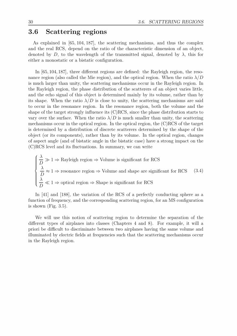
30 3.6. SCATTERING REGIONS

3.6 Scattering regions

As explained in [65, 104, 187], the scattering mechanisms, and thus the complexand the real RCS, depend on the ratio of the characteristic dimension of an object,denoted by D, to the wavelength of the transmitted signal, denoted by λ, this foreither a monostatic or a bistatic configuration.

In [65, 104, 187], three different regions are defined: the Rayleigh region, the reso-nance region (also called the Mie region), and the optical region. When the ratio λ/Dis much larger than unity, the scattering mechanisms occur in the Rayleigh region. Inthe Rayleigh region, the phase distribution of the scatterers of an object varies little,and the echo signal of this object is determined mainly by its volume, rather than byits shape. When the ratio λ/D is close to unity, the scattering mechanisms are saidto occur in the resonance region. In the resonance region, both the volume and theshape of the target strongly influence its (C)RCS, since the phase distribution starts tovary over the surface. When the ratio λ/D is much smaller than unity, the scatteringmechanisms occur in the optical region. In the optical region, the (C)RCS of the targetis determined by a distribution of discrete scatterers determined by the shape of theobject (or its components), rather than by its volume. In the optical region, changesof aspect angle (and of bistatic angle in the bistatic case) have a strong impact on the(C)RCS level and its fluctuations. In summary, we can write

λ

D≫ 1 ⇒ Rayleigh region ⇒ Volume is significant for RCS

λ

D≈ 1 ⇒ resonance region ⇒ Volume and shape are significant for RCS

λ

D≪ 1 ⇒ optical region ⇒ Shape is significant for RCS

(3.4)

In [41] and [188], the variation of the RCS of a perfectly conducting sphere as afunction of frequency, and the corresponding scattering region, for an MS configurationis shown (Fig. 3.5).

We will use this notion of scattering region to determine the separation of thedifferent types of airplanes into classes (Chapters 4 and 8). For example, it will apriori be difficult to discriminate between two airplanes having the same volume andilluminated by electric fields at frequencies such that the scattering mechanisms occurin the Rayleigh region.

3.7. BS-RCS OF A PERFECTLY CONDUCTING SPHERE 31

Figure 3.5: RCS of a perfectly conducting sphere as a function of the ratio of itscircumference to the wavelength. The three scattering regions are also shown [188].

3.7 Computation of the bistatic RCS of a simple

object, the perfectly conducting sphere

In the previous sections, we investigated the mechanisms responsible for the echosignal, and thus the bistatic radar cross-section (BS-RCS) and the bistatic complexradar cross-section (BS-CRCS) of a target. It was intuitively shown that the natureof the target, the aspect angle at which it is viewed, the frequency of the incidentwave, and the bistatic angle between the transmitter (Tx) and the receiver (Rx) areparameters that influence the value of both the BS-RCS and the BS-CRCS.

In order to completely define the parameters that the BS-CRCS and the BS-RCSdepend on, and to provide physical insight into the nature of the BS-RCS, we derive,in this section, the exact expression for the BS-RCS of the perfectly conducting sphere.Given the complexity of the derivation for an object as simple as a sphere, it is easyto understand that it is difficult to derive the exact expression for the BS-RCS of acomplex object in an analytical way. This derivation will show that the theoreticalformulation of the BS-RCS of a complex target is difficult to obtain. The derivationis similar for the BS-CRCS.

The derivation of exact and approximated expressions for the BS-RCS of ob-jects is performed in [49, 180, 182, 194, 195]. We give here the main steps for thederivation of the exact expression for the BS-RCS of a generic object, so that thisexpression can be discussed in terms of its parameters, exactly as in [50,65,98,181,188].

The geometry considered is the one described in Section 3.3. An electromagneticfield is transmitted by a Tx, considered to be a point source. The electromagneticfield is scattered by the target, and then collected by an Rx. According to Eqs. (3.1)and (3.2), in order to compute either the BS-CRCS or the BS-RCS of the object,we have to compute either the ratio of the received electric field (E-field) to the

32 3.7. BS-RCS OF A PERFECTLY CONDUCTING SPHERE

transmitted E-field, or the ratio of the received magnetic field (H-field) to thetransmitted H-field. Even though we can use either the H-field or the E-field, we adoptthe common convention of using the H-field in the computations below [49, 180, 182].Therefore, the computations below aim at expressing the received H-field in terms ofthe transmitted H-field.

In Section 3.6, we showed that both the BS-CRCS and the BS-RCS depend onthe scattering region (Rayleigh, resonance, or optical). As will be seen in Chapters 4and 8, the scattering mechanisms of the air targets that we classify occur mainly inthe optical region, i.e. when the characteristic dimension D of a target is much greaterthan the wavelength λ of the transmitted and scattered signals. Therefore, we willuse the physical optics approximation when possible, exactly as in [180, 182]. Theuse of the physical optics approximation is justified in [182]. The computation of theRCS of generic targets in the Rayleigh and resonance scattering regions can be foundin [50,180]. Other RCS prediction techniques, such as numerical methods, can be foundin [188].

3.7.1 Hypotheses

We perform the derivation of the expression for the BS-RCS under four common as-sumptions [49,182,194,195]. First, we assume the far-field conditions are met. Second,we assume that the waves transmitted by any transmission source are plane in the far-field [212]. Third, we assume that the generic object for which the BS-RCS is derivedis perfectly conducting. Fourth, we assume that the scattering surface dimensions arelarge compared to the wavelength of the incident wave. Below, we explain the first twoassumptions.

Far-field condition

Three spatial regions around a transmitter are defined: the reactive near-field region,the near-field region, also called the Fresnel region, and the far-field region, also calledthe Fraunhofer region [8,23,109]. We consider the far-field region for the derivation ofthe expression of the BS-RCS. In [8,23,109], the far-field region is defined as the regionof space where the angular field distribution is, for all practical purposes, independentof the distance from the antenna. The far-field region is reached when the followingthree conditions are all met:

rT >2D2

λ

rR >2D2

λ

D ≥ λ,

(3.5)

where D is the characteristic dimension of the target, λ is the wavelength of thetransmitted signal, and rT and rR the distances from the target to the Tx and the Rx,respectively.

We consider the far-field region, since it will be the case of the subsequent config-urations considered. For example, in Chapter 8, the characteristic dimension of thelarge-size airplanes for which the BS-RCS is computed is 65 m at most, and the wave-length of the transmitted signal is 3×108/(114.7×106) = 2.616 m. Therefore, in orderto satisfy the far-field condition, rT and rR must be at least 3.23 km, which is the case

3.7. BS-RCS OF A PERFECTLY CONDUCTING SPHERE 33

for the configuration used, as described in Chapter 8. Of course, the characteristic di-mension D = 65 m is greater than the wavelength λ = 2.616 m. The far-field conditionis thus satisfied.

Plane waves

Being in the far-field region allows one to use the hypothesis of plane waves. Theplane wave assumption is explained as follows. We assume that the signal emitted by apoint source, denoted here by Tx, is monochromatic, and isotropic (Fig. 3.6). We alsoassume that the transmitted signal has a constant amplitude. We can thus expressthe transmitted signal st(t), with superscript t standing for "transmit", via a periodiccomplex exponential

st(t) = Aejωt, (3.6)

where A represents the constant amplitude of the signal, and ω the (constant)pulsation of the signal, related to its frequency via ω = 2πf . Note that we will oftenabusively refer to ω as the frequency of the signal. Also note that ω, and thus f , aresigned quantities.

For simplicity, we perform the development below in a two-dimensional (2D) plane.One can easily extend it to a three-dimensional space. Around the point source, weassume that the front wave is circular, since the point source is assumed to be isotropic.The plane wave condition means that, at a distance large enough from the point source,both the amplitude and the the phase of the signal are the same for all points on any linesegment perpendicular to the direction of propagation of the signal, i.e. the wavefront.For example, as shown in Fig. 3.6, both the amplitude and the phase of the signal st(t)at points P1 and P2 are the same, under the plane wave condition.

b

b

b

b b bTx

P1

P2

st(t)

Figure 3.6: Illustration of the plane wave condition.

3.7.2 Transmitted electric and magnetic fields

The electric field (E-field) transmitted by a monochromatic point source Tx can beexpressed as [108]

Et(r, t) = E0(r)e

j(ωt−k· r), (3.7)

where E0 is the amplitude of the field, ω the pulsation, k the wave vector, and r aposition vector in R3.

At any point P , the E-field can be expressed as [108]

E(rP , t) = E0(rP )e−jk· rP ejωt = E(rP )ejωt. (3.8)

34 3.7. BS-RCS OF A PERFECTLY CONDUCTING SPHERE

In Eq. (3.8), E(rP , t), E(rP ), and ejωt are complex-valued. E(rP ) is a complex numberthat is specific to point P . It is multiplied by the complex exponential ejωt to producethe time-varying complex-valued representation of the E-field at P , i.e. E(rP , t).E(rP , t) is a complex value that varies with time (for a given location) and withlocation (for a given time).

From a signal processing point of view, the multiplication of E(rP ) by ejωt

can usefully be interpreted as the rotation of the fixed complex number E(rP )by an angle ωt in the complex plane, as illustrated in Fig 3.7. Therefore, theE-field representation, which is defined in Eq. (3.8) as being the product of E(rP )by ejωt, can be viewed as a vector of length |E(rP )| rotating at angular speed ωin the complex plane, starting at angle ∠E(rP ) (the phase of E(rP )) at t = 0.E(rP ) and E(rP , t) are both called phasors. We will refer to E(rP ) as a fixed pha-sor, and to E(rP , t) as a time-varying phasor or, more specifically, as a rotating phasor.

Re

Im

E(rP , t = 0)E(rP , t)

|E(rP )|

∠E(rP )

ωt

E(rP , t)

Figure 3.7: Representation of E(rP , t) in the complex plane.

Carefully note that, to determine the complex value of E(rP , t) at a given pointP, and for all t’s, we only need to know the fixed phasor E(rP ) specific to point P(and of course, ω). Note that E(rP ) is not completely arbitrary. If the direction ofpropagation k of the plane wave and the value of E(rP ) at some point such as theorigin O are known, the value of E(rP ) can be automatically determined for all pointsP in the (x, y, z) axes.

Of course, in real life, all physical electric fields are real-valued. But the actual valueof the physical E-field can be obtained by projecting, at any time t, the complex-valuedrotating phasor E(rP , t) on the real axis of the complex plane. This means that thereal-valued physical E-field, which is denoted by E(rP , t), is also simply the real part

3.7. BS-RCS OF A PERFECTLY CONDUCTING SPHERE 35

of the rotating phasor E(rP , t),

E(rP , t) = ℜ{E(rP , t)} = ℜ{E(rP )ejωt}, (3.9)

as illustrated in Fig. 3.7. Observe that we use E for the complex-valued E-field andE for the corresponding physical real-valued E-field. Below, we deal with both theelectric field and the magnetic field. We can similarly express the H-field transmittedby a point source as

Ht(r, t) = H0(r)e

j(ωt−k· r), (3.10)

and one can make the same reasoning as for the E-field.

3.7.3 Scattered electric field

We derive the expression for the scattered electric field (E-field) according to [49,182, 194,195]. The derivation starts from the Maxwell equations [23, 109, 194]

∇ × E = −∂B

∂t, (3.11)

∇ × H =∂D

∂t+ J , (3.12)

∇ · D = ρ, (3.13)

∇ · B = 0, (3.14)

where E represents the electric field, B the magnetic induction, H the magnetic field,D the electric displacement, J the current density, and ρ the charge density. Byassuming an harmonic time dependence of E and H of the form of ejωt, and by assumingan homogeneous, isotropic, and source-free region, E and H both satisfy the waveequation [23, 49, 109, 182,194,195]

(∇2 + k2

)ψ = 0, (3.15)

where ψ can represent either E or H.

At the interface of two perfect dielectrics, the boundary conditions of continuitycan be expressed as

n× (E1 − E

2) = 0 (3.16)

n× (H1 − H

2) = 0 (3.17)

n· (D1 − D

2) = 0 (3.18)

n· (B1 − B

2) = 0, (3.19)

where n stands for the normal unit vector, and the superscripts 1 and 2 stand for eachside of the interface, as shown in Fig. 3.8.

Since we assume that the object is perfectly conducting, we have

n× E = 0 (3.20)

n· B = 0. (3.21)

36 3.7. BS-RCS OF A PERFECTLY CONDUCTING SPHERE

y

z

x

Object O

n

B2

D2

H2

E2

E1

H1

B1

D1

Figure 3.8: Simplified illustration of the different electric and magnetic fields at theinterface between two perfect dielectrics.

Since we assume an incident plane wave, both E and H are of the form

ψ = ψI

+ ψS, (3.22)

where the superscripts I and S stand for the incident and scattered fields, respectively.The general solution of Eq. (3.15), expressed in its scalar form, is [49]

ψ(r) = ψI(r) +∫

S

(f∂G

∂n− gG

)dS, (3.23)

where f = ψ and g = ∂ψ/∂n. In the case of E and H , and by using the boundaryconditions of Eq. (3.19), one can get [49]

E = EI

+1ik

∇ ×∫

S∇G×

(n× H

)dS, (3.24)

H = HI −

∫

S∇G×

(n× H

)dS, (3.25)

where G is the Green function defined by

G(r, r′) =1

4πe−jk|r−r′|

|r − r′| , (3.26)

where r is the distance vector from the center of the coordinate system to the observa-tion point, i.e. the receiver, and r′ the distance vector from the center of the coordinatesystem to the integration point on the surface S of the object. We can rewrite this lastexpression as

G(R) =1

4πe−jk|R|

|R| , (3.27)

where R = r − r′. The gradient of the Green function is written as

∇G =1

4π

(−jke

−jkR

R− e−jkR

R2

)R (3.28)

=1

4π

(−jke

−jk(r−r′)

r − r′ − e−jk(r−r′)

(r − r′)2

)r. (3.29)

3.7. BS-RCS OF A PERFECTLY CONDUCTING SPHERE 37

Since the distance r is very large, one can approximate the gradient of the Greenfunction as

∇G ≈ −ejkr

4πrjkre−jkr· r′

(3.30)

We can thus express the scattered electric and magnetic fields as [49]

ES

= −ejkr

4πrr∇ ×

∫

Se−jkr· r′ ×

(n× H

)dS (3.31)

HS

=ejkr

4πrjkr ×

∫

Se−jkr· r′

(n × H

)dS. (3.32)

In [182], the scattered magnetic field HS

is equivalently expressed as

HS

=1

4π

∫

S

(n× H

)× ∇

(e−jkR

R

)dS, (3.33)

where n still denotes the unit vector normal to the surface S, k is still the wavenumber, and S is the integration region, which is the outer surface of the object. R isnow the distance from the observation point, i.e. the receiver, to the integration pointon S. H denotes the tangential component of the magnetic field on the surface of theobject.

Since we assume that the dimensions of the surface of the object are large comparedto the wavelength, we can use the physical optics approximation as in [182] to expressthe magnetic field H as

H =

2iTH0e

−jk· r, on the illuminated side of the object

0, otherwise,, (3.34)

where iT = a − (a· n)n, where a represents the direction of propagation of theincident magnetic field, H0 stands for the magnitude of the incident magnetic field, kthe wave number vector, and r the distance vector from the origin of the coordinatesystem to any point on the surface of the object.

By using Eq. (3.30), and assuming H0 = 1, we get [182]

HS

=e−jkR′

R′ F (β), (3.35)

where R′ is the distance from the center of the coordinate system to the receiver, andwhere F (β) is expressed as

F (β) =jk

2π

[(n0 · a) f −

(n0 · f

)a], (3.36)

where n0 is the unit vector from the receiver to the origin, and f is defined as

f =∫

S′

ne−jkr· (n0+k)dS, (3.37)

where S ′ stands for the illuminated side of the object.

38 3.7. BS-RCS OF A PERFECTLY CONDUCTING SPHERE

By using Eq. (3.2), we can thus express the BS-RCS of the object as

σ(β) = 4π|F (β)|2. (3.38)

The dependence of the BS-RCS on the aspect angle, the bistatic angle, and thefrequency appears through the definition of f (Eq. (3.37)). More precisely, thedependence of the BS-RCS on the aspect angle appears through the vector r. Thedependence of the BS-RCS on the bistatic angle is expressed through the addition ofthe vectors n0 and k. This dependence is discussed in Section 3.7.4. The dependenceof the BS-RCS on the frequency f comes through the wave number k = 2π/λ = 2πf/c.

Up to now, we have not introduced the polarization of the incident and scatteredelectromagnetic fields. In [182], the polarization of the receiver is introduced throughunit vector d. We thus express the BS-RCS as

σ(β) = 4π|F · d|2

=4πλ2

∣∣∣(n0 · a)(f · d

)−(n0 · f

) (a· d

)∣∣∣2. (3.39)

In order to analytically determine the BS-RCS of any object, Eq. (3.37) requires thatone be able to give an analytical expression for the outer surface of the object. While itis possible to give an analytical expression for the scattering surface of simple objectssuch as spheres, spheroids, or cones, it is, however, extremely difficult, if not impossible,to give such expression for complex objects, such as airplanes. For illustration purposes,we present the simple example of a sphere in Section 3.7.5.

3.7.4 Bistatic complex RCS and bistatic RCS as a function of

the bistatic angle

The bistatic geometry is characterized by the bistatic angle β [91]. We showed inSection 3.7.3 that the BS-CRCS and the BS-RCS depend on the value of the bistaticangle β, among other parameters.

In [188], three different regions of bistatic RCS are defined, according to the valueof the bistatic angle: the pseudo-monostatic RCS region, the bistatic RCS region, andthe forwardscatter RCS region. The pseudo-monostatic RCS region corresponds toβ ≤ 5◦. In this region, one can compute the BS-RCS by using the monostatic-bistaticequivalence theorem (MBET), as shown in Section 3.8. The MBET states that theBS-RCS of an object is equal to its monostatic RCS measured at an aspect angleequal to β/2, and at a frequency equal to f csc(β/2).

The bistatic RCS region corresponds to 5◦ ≤ β ≤ 180◦. When the bistatic angle ishigher than 5◦, the monostatic-bistatic equivalence theorem can no longer be applied.The reasons, explained in [98, 188], are that the relative phases between the different(discrete) scatterers constituting the object change, and that the amplitude and phaseof the different scatterers vary according to the bistatic angle. To our knowledge, notheoretical model for the computation of the BS-RCS of a complex object exists forthe bistatic RCS region.

3.7. BS-RCS OF A PERFECTLY CONDUCTING SPHERE 39

The forwardscatter RCS region corresponds to β → 180◦. Around this value of thebistatic angle, it is shown in [181] that the BS-RCS of an object is equal to 4πA2/λ2,where A is the effective area of the object. Methods for predicting the forwardscatterRCS of different targets are discussed in [43, 184, 185]. The recognition of objectsbased on their forwardscatter RCS is discussed in [39, 40].

For illustration purposes, and in preparation for Chapter 8, we compute theBS-RCS of a sample airplane as a function of the azimuth aspect angles with respectto the transmitter and the receiver, denoted by θTx and θRx, respectively. The modelof the airplane consists of a fuselage of size 5.42m × 1m, and two wings of size2.58m × 1m. A stationary current runs through the fuselage and the wings. Figure 3.9shows the BS-RCS of this airplane at a frequency of 115 MHz. As explained above,when θTx + θRx ≈ 180◦, i.e. in forwardscattering, the BS-RCS of the airplane ismaximum, constant, and equal to 10 log(4πA2/λ2) ≈ 20 dB.

One can also see in Fig. 3.9 that, for the pseudo-monostatic region, when thebistatic angle β is small, i.e. when θTx ≈ θRx (on the anti-diagonal of the graph), thevalue of the csc(β/2) is small, and therefore the amplitude of the BS-RCS does notvary much. The variations are much noticeable for large bistatic angles, but smallerthan 180◦.

Figure 3.9: RCS of a sample airplane as a function of its aspect angles with respectto the transmitter and the receiver, denoted by θTx and θRx, respectively.

In this work, we focus on the bistatic RCS region. Since the BS-RCS of complexobjects cannot be easily predicted by any theoretical model, there is a crucial need forexperimental data. Moreover, since we focus on the recognition of such complex objects,the amount of data must be sufficient, in order to perform meaningful classificationexperiments.

40 3.7. BS-RCS OF A PERFECTLY CONDUCTING SPHERE

3.7.5 Application to the case of the perfectly conductingsphere

In this section, we compute the BS-RCS of a sphere of radius R0, from the equationsderived in Section 3.7.3. Since the sphere is a symmetric object in all directions, onecan intuitively understand that its BS-RCS does not depend on the aspect angle.

As in [49,182], and as shown in Fig. 3.10, we assume that the transmitter is locatedat T , on the positive side of the z-axis, thus resulting k = −iz. We also assume thatthe direction of propagation a of the incident magnetic field is directed along they-axis. We assume that the receiver is located at R, in the yz-plane, and that itspolarization is directed along the y-axis, iy. The sphere is located at O.

y

z

x

O

b

b

n

r

k

a

n0

TR

r

r′

α0dS

β

Figure 3.10: Configuration used for the theoretical computation of the BS-RCS of asphere, as in [49,182].

Under these assumptions (and those used from Section 3.7.1 to Section 3.7.3), it isshown in [181,182] that, for a prolate spheroid with major axis a and minor axis b, theinner part of Eq. (3.39) is equal to

2πb2∫ 1

0

∫ 2π

0ηe

−j(kb sinβ

√1−η2 sinφ−ka(1+cos β)−ka(1+cos β)η

)

dφdη, (3.40)

where η and φ are the (angular) spherical coordinates of a generic point on the prolatespheroid. By using the fact that [1]

∫ 2π

0e−jkψ sinφdφ = 2πJ0(kψ), (3.41)

where J0 is the zero-order Bessel function, and by performing the change of variablesη = sin θ, Eq. (3.40) becomes

2πb2∫ π/2

0sin θ cos θJ0(kb sin β sin θ)ejka(1+cos β) cos θdθ. (3.42)

In the case of a sphere, a = b = R0, and the expression reduces to

2πR20

∫ π/2

0sin θ cos θJ0(kR0 sin β sin θ)ejkR0(1+cos β) cos θdθ. (3.43)

3.7. BS-RCS OF A PERFECTLY CONDUCTING SPHERE 41

The BS-RCS of the sphere is thus equal to

σ(β) =4πλ2

4π2R20

∣∣∣∣∣

∫ π/2

0sin θ cos θJ0(kR0 sin β sin θ)ejkR0(1+cos β) cos θdθ

∣∣∣∣∣ . (3.44)

As explained in [181, 182], this integral is evaluated by the double stationary phasetheorem, which is applicable when the characteristic dimension D of the object ismuch larger than the wavelength of the incident field (physical optics approximation).The results achieved is exactly the same as the result achieved by geometrical optics.In the case of the prolate spheroid, we get

σ(β) ≈ 4πb4

a2

((1 + cosβ +

b2

a2(1 − cosβ)

)−2

. (3.45)

In the case of the sphere, a = b = R0, and we thus get

σ(β) ≈ πR20. (3.46)

One must notice that the bistatic angle β does not appear on the right-hand side ofthis equation. In [182], a comparison with measured BS-RCSs of a sphere shows thatthe result of Eq. (3.46) is valid for bistatic angle smaller than 120◦.

3.7.6 Bistatic RCS of canonical objects

In Section 3.7.5, we presented the theoretical computation of the sphere, which isa particular canonical object. In this section, we list the BS-RCS values for othercanonical objects, computed under the same assumptions as those used for the sphere.

The BS-RCS of the finite cone of length r0 and half cone angle γ is expressedin [181, 182] as

σ(β) ≈ 4πr20 sin(4γ)

(sin2 β sin2 γ − cos2 γ(1 + cosβ)2)2

[cos γ(1 + cosβ)J2

0 (kr0 sin β sin γ)+

sin2 β sin2 γJ21 (kr0 sin β sin γ)

].

(3.47)

Similarly, the BS-RCS of the paraboloid defined by

x2 + y2 = −4Pz (3.48)

is expressed as [181, 182]σ(β) = 4πP 2 sec4 (β/2) . (3.49)

The BS-RCS of the ellipsoid defined by

x2

A2+y2

B2+z2

C2= 1 (3.50)

is expressed as [181, 182]

σ(β) =4πA2B2

C2

[(1 + cosβ) +

B2

C2(1 − cos β)

]−2

. (3.51)

One can find expressions for the BS-RCS of other canonical objects in [181,182]. Com-parisons with measurements of BS-RCS of objects are available in [41,49,224,225]. Inall cases considered in this section, the BS-RCS σ depends explicitly on the bistaticangle β.

42 3.8. MONOSTATIC-TO-BISTATIC EQUIVALENCE THEOREMS

3.8 Monostatic-to-bistatic equivalence theorems

In Section 3.7, we presented the theoretical computation of the bistatic radarcross-section (BS-RCS) of a perfectly conducting sphere. The main difficulty lied inthe analytical formulation of the shape of the object. Another way of getting theBS-RCS of an object is to obtain its value from its monostatic radar cross-section(MS-RCS), which is the purpose of the monostatic-to-bistatic equivalence theorem(MBET).

In [98], Kell proposed the following MBET for relatively smooth objects

σBS(θ = β, f) = σMS

(θ =

β

2, f csc

(β

2

)), (3.52)

where σBS represents the BS-RCS, σMS the MS-RCS, θ the azimuth angle of theobject, β the bistatic angle, and f the frequency.

In [48], Crispin and Siegel proposed another MBET, extended for complex objects,

σBS(θ = β, f) = σMS

(θ =

β

2, f

), (3.53)

which is identical to Eq. (3.52) for β = 0.

Eigel performed the analysis of both MBET’s on three simple objects: a plate andtwo cylinders mounted on a base [65]. Eigel showed that both MBET’s start to fail atbistatic angles larger than 20◦, mainly due to the change of scattering centers growingwith increasing bistatic angle. One can find a more thorough analysis of MBET’sin [41]. Because of this limitation, we will not use MBET’s to obtain the BS-RCSs ofcomplex objects such as airplanes.

3.9 Conclusion

Our three automatic target recognition (ATR) systems, that we further discuss inChapters 6, 7, and 8, all use either the bistatic complex radar cross-section (BS-CRCS)or the bistatic radar cross-section (BS-RCS). In this chapter, we defined these twoquantities, and we identified the parameters they depend on.

In particular, we defined the BS-CRCS and of BS-RCS in terms of the transmittedand scattered electromagnetic fields. We presented the different scattering mechanismsthat are responsible for both the BS-CRCS and the BS-RCS. We also defined the threescattering regions: the Rayleigh region, the resonance region, and the optical region.The dominant scattering mechanisms that contribute to both the BS-CRCS and theBS-RCS of an object differ according to the ratio of the characteristic dimension ofthe object to the wavelength of the transmitted electromagnetic field. In particu-lar, the separation of targets into different classes in our three ATR systems relieson the determination of the scattering region in which the scattering mechanisms occur.

3.9. CONCLUSION 43

We also defined the different bistatic RCS regions, according to the value ofthe bistatic angle β: the pseudo-monostatic region, the bistatic region, and theforwardscatter region. We illustrated the variations of the BS-RCS as a function ofthe bistatic angle on a simple model of a small airplane.

The BS-RCS depends on the following parameters: the nature of the object, theaspect angle of this object with respect to either the transmitter or the receiver,the bistatic angle between the transmitter and the receiver, the polarizations of thetransmitter and the receiver, and the frequency of the illuminating wave. Our threeATR systems all take advantage of the analysis of the variation of either the BS-CRCSor the BS-RCS in terms of these parameters. In order to illustrate the influenceof these parameters on the BS-RCS, we presented the theoretical computation ofthe BS-RCS of the simple perfectly conducting sphere, under the physical opticsapproximation. We showed that the theoretical computation of the BS-RCS of ageneric target requires the analytical expression of its shape. Since this analyticalexpression is not available for complex objects, the geometry of complex objects isoften discretized by an ensemble of canonical shapes, such as spheres or dihedrals. Itfollows that the BS-CRCS and BS-RCS of such targets cannot be computed exactly,and that their computation requires either a large amount of time or a large amountof computational resources.

We also expressed the limitations of the monostatic-to-bistatic equivalence theoremsthat aim at computing the BS-RCS of an object from the values of the monostaticRCS of this object. These theorems will thus not be used for the computation of theBS-RCSs of complex objects such as airplanes. Therefore, since a large amount of datais needed to perform meaningful classification experiments, we will put a particulareffort, in Chapters 4 and 8, into the collection of a sufficient amount of data.

44 3.9. CONCLUSION

Chapter 4

Extraction and illustrations of thebistatic complex and real RCS oftargets

Contents4.1 Motivation . . . . . . . . . . . . . . . . . . . . . . . . . . . . 46

4.2 Extraction of the BS-CRCS and the BS-RCS of targets . 47

4.2.1 Transmitted electric field . . . . . . . . . . . . . . . . . . . . 47

4.2.2 Polarization . . . . . . . . . . . . . . . . . . . . . . . . . . . . 48

4.2.3 Expressions for the Tx and Rx E-fields . . . . . . . . . . . . . 50

4.2.4 Bistatic polarization scattering matrix . . . . . . . . . . . . . 52

4.2.5 Components of the bistatic polarization scattering matrix . . 53

4.2.6 Bistatic complex RCS . . . . . . . . . . . . . . . . . . . . . . 55

4.2.7 Bistatic polarization CRCS matrix . . . . . . . . . . . . . . . 56

4.2.8 Position of the Tx as reference for the Tx electric field . . . . 57

4.2.9 Case of a single linear polarization . . . . . . . . . . . . . . . 58

4.2.10 Practical measurement of the BS-RCS of targets . . . . . . . 59

4.3 Acquisition of raw data: experimental setup . . . . . . . . 59

4.3.1 Motivation for using scaled models in an anechoic chamber . 59

4.3.2 Configuration geometry . . . . . . . . . . . . . . . . . . . . . 60

4.3.3 Acquisition of raw data . . . . . . . . . . . . . . . . . . . . . 61

4.3.4 Airplanes of interest . . . . . . . . . . . . . . . . . . . . . . . 63

4.4 Scattering regions . . . . . . . . . . . . . . . . . . . . . . . . 65

4.5 Classes of airplanes . . . . . . . . . . . . . . . . . . . . . . . 65

4.6 Illustration of the BS-CRCS and the BS-RCS of targets . 66

4.6.1 BS-CRCS as a function of the bistatic angle . . . . . . . . . . 66

4.6.2 BS-CRCS as a function of the frequency . . . . . . . . . . . . 69

4.6.3 BS-CRCS as a function of the polarization . . . . . . . . . . 73

4.6.4 BS-CRCS as a function of the orientation . . . . . . . . . . . 73

45

46 4.1. MOTIVATION

4.6.5 Conclusions about the variations of BS-CRCS . . . . . . . . . 75

4.7 Conclusion . . . . . . . . . . . . . . . . . . . . . . . . . . . . 77

In this chapter, we extract both the bistatic complex radar cross-section (BS-CRCS)and the bistatic radar cross-section (BS-RCS) of targets from the transmitted andreceived electric fields. We also describe the experimental setup used to collect thereceived electric fields. We then illustrate the variations of both the BS-CRCS andthe BS-RCS as a function of the parameters investigated in Chapter 3.

Section 4.1 states the motivation for the extraction of both the BS-CRCS andthe BS-RCS. Section 4.2 presents the computation of both the BS-CRCS and theBS-RCS of a generic target from the transmitted and received electric fields. Section 4.3presents the experimental setup we used for the extraction of both the BS-CRCS andthe BS-RCS of targets. Section 4.4 defines the scattering regions in the frequency bandsof interest. Section 4.5 defines the classes of targets to classify. Section 4.6 illustratesthe variations of both the BS-CRCS and the BS-RCS as a function of the differentparameters that we described in Chapter 3. Section 4.7 concludes.

4.1 Motivation for the extraction of the bistatic

complex and real RCS of targets

Our first automatic target recognition system (ATR), whose block diagram is shownin Fig. 4.1, recognizes targets by using their radar image. We compute the radarimages of targets from the bistatic complex radar cross-section (BS-CRCS) of thesetargets (Chapter 5). Our second ATR system, whose block diagram is representedin Fig. 4.2, recognizes targets by using either their BS-CRCS or their bistatic radarcross-section (BS-RCS).

Figure 4.1: Block diagram of our ATR system using radar images of targets.

We consider, in this chapter, the first stage of these two ATR systems, which is theextraction of either the BS-CRCS or the BS-RCS of targets, for both the learning set(LS) and the test set (TS).

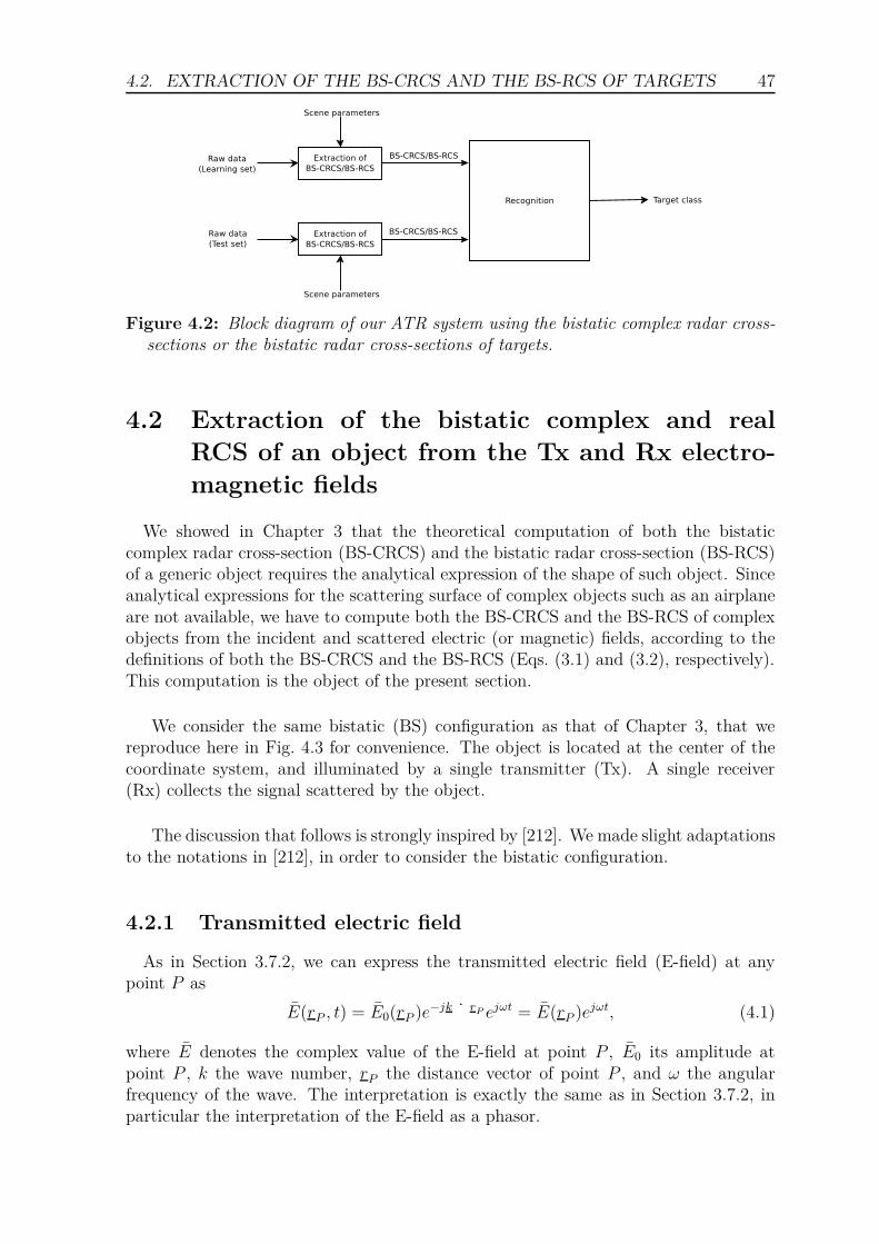
4.2. EXTRACTION OF THE BS-CRCS AND THE BS-RCS OF TARGETS 47

Figure 4.2: Block diagram of our ATR system using the bistatic complex radar cross-sections or the bistatic radar cross-sections of targets.

4.2 Extraction of the bistatic complex and real

RCS of an object from the Tx and Rx electro-

magnetic fields

We showed in Chapter 3 that the theoretical computation of both the bistaticcomplex radar cross-section (BS-CRCS) and the bistatic radar cross-section (BS-RCS)of a generic object requires the analytical expression of the shape of such object. Sinceanalytical expressions for the scattering surface of complex objects such as an airplaneare not available, we have to compute both the BS-CRCS and the BS-RCS of complexobjects from the incident and scattered electric (or magnetic) fields, according to thedefinitions of both the BS-CRCS and the BS-RCS (Eqs. (3.1) and (3.2), respectively).This computation is the object of the present section.

We consider the same bistatic (BS) configuration as that of Chapter 3, that wereproduce here in Fig. 4.3 for convenience. The object is located at the center of thecoordinate system, and illuminated by a single transmitter (Tx). A single receiver(Rx) collects the signal scattered by the object.

The discussion that follows is strongly inspired by [212]. We made slight adaptationsto the notations in [212], in order to consider the bistatic configuration.

4.2.1 Transmitted electric field

As in Section 3.7.2, we can express the transmitted electric field (E-field) at anypoint P as

E(rP , t) = E0(rP )e−jk· rP ejωt = E(rP )ejωt, (4.1)

where E denotes the complex value of the E-field at point P , E0 its amplitude atpoint P , k the wave number, rP the distance vector of point P , and ω the angularfrequency of the wave. The interpretation is exactly the same as in Section 3.7.2, inparticular the interpretation of the E-field as a phasor.

48 4.2. EXTRACTION OF THE BS-CRCS AND THE BS-RCS OF TARGETS

b b

b

T

R

P

φ

θ

rP

y

z

x

rR

rT

Object

β

OkT

φt

θt

θr

φr

rT

rR = kR

rP

p

p

p

p

Figure 4.3: Geometry of the bistatic configuration considered.

4.2.2 Polarization

In contrast to the theoretical computation of the BS-RCS, we introduce thepolarization of the incident and scattered electric fields from the start. For sim-plicity, we start with linear polarization. If an electromagnetic field (EM-field),or wave, is linearly polarized, the polarization is necessarily characterized by anorientation in space, i.e. in the (x, y, z) axes of Fig. 4.3. As is customary, wechoose the orientation of the electric field E to characterize the orientation of the po-larization [108]. Alternatively, one could choose the orientation of the magnetic field H .

In the case of a propagating plane wave characterized by its wave vector k, and thustravelling in the direction of k (and k), we know that the electric field E (E-field) andthe magnetic field (H-field) are perpendicular to k. The unit vector p characterizingthe orientation of the linearly polarized E-field E is shown in Fig. 4.3. We show p"attached" not only to O but also to Tx, to Rx, and to some arbitrary point P . In anycase, p can be thought of as being located in the plane perpendicular to the directionof propagation k.

A linearly-polarized E-field is characterized by the direction p of its polarization,and by its real-valued amplitude E(rP , t). The corresponding E-field vector in the(x, y, z) axes is denoted by E(rP , t) and given, by inspection and construction, by

E(rP , t) = E(rP , t)p. (4.2)

Keep in mind that E and p are three-element vectors in the (x, y, z) axes.

Before moving on, it is critical to have a crystal-clear view of the notations used sofar, and of the quantities they represent.

• p represents the direction of polarization, which is assumed linear. It is a unitvector in the (x, y, z) axes, i.e. in R3. As all vectors of R3, it has three elementsand these are real-valued.

• rP is the position vector of some point P. It is a vector in the (x, y, z) axes, i.e.in R3.

4.2. EXTRACTION OF THE BS-CRCS AND THE BS-RCS OF TARGETS 49

• E(rP , t) is the real value (i.e. the time-varying amplitude) of the linearly polar-ized E-field vector at location rP , i.e. at P, and at time t.

• E(rP , t) is the real value of the physical E-field vector at rP and t, characterizedby the orientation p and the physical (real-valued, scalar) time-varying amplitudeE(rP , t). It is a vector in the (x, y, z) axes, i.e. in R3.

• E(rP , t) is the complex time-varying rotating phasor representation of the valueof the time-varying amplitude E(rP , t). It rotates counterclockwise at angularspeed ω. It is a complex number in the complex plane C. As any complex number,it can also be viewed as a two-element vector with real-valued components (itsreal and imaginary parts), and thus as a vector in R2.

• E(rP ) is a fixed phasor corresponding to E(rP , t). It is a fixed complex number.It can also be viewed as a two-element vector with real-valued components, andthus as a vector in R2.

Horizontal and vertical linear polarizations

The horizontal polarization (often denoted by H) and the vertical polarization(often denoted by V ) are perhaps the most fundamental and the most common typesof linear polarization. (Please do not mix up the symbol H used for both the magneticfield and the horizontal polarization.) Furthermore, other types of polarization, suchas circular polarization, are naturally described as the proper combinations of some Hand V polarizations [108].

To define the linear H polarization and the linear V polarization, we simply needto indicate what the corresponding vectors p in the (x, y, z) axes are. With referenceto Fig. 4.3, we have

p = φ for H polarization

p = θ for V polarization,

where the unit vectors φ and θ are defined as follows. θ is the unit vector "located" inthe plane defined by the z-axis and the direction of propagation k, perpendicular to k,and oriented in the positive sense of the (polar) angle θ. φ is the unit vector "located"in the horizontal plane, perpendicular to k, and oriented in the positive sense of the(azimuth) angle φ.

Carefully note that the direction φ of horizontal (H) polarization and the directionθ of vertical (V ) polarization form a right-handed system of axes with k = −r, but notwith r. This is perfect since what really matters from an electromagnetic standpointis the direction of propagation (i.e. k) and the directions of the H and V polarizations.

It should be noted that, while φ is oriented parallel to the horizontal plane, andis thus horizontal, θ is not oriented vertically. However, θ is in a vertical plane. Oneshould thus be careful concerning the meaning of the qualifiers "horizontal" and "verti-cal" when talking about polarization. The V polarization is generally not vertical, andit could be horizontal if k is aligned with the z-axis. A particular case is when φ is in

50 4.2. EXTRACTION OF THE BS-CRCS AND THE BS-RCS OF TARGETS

the horizontal plane, and when the receiver is at a long distance from the target. Inthis case, θ is vertical.

Arbitrary linear polarizations

We have indicated that the orientation vector p of a given linear polarization is nec-essarily perpendicular to the direction of propagation k. This means that this vectorp is in the plane defined by φ (H polarization) and θ (V polarization). Therefore,the real-valued E-field vector corresponding to an arbitrary linear polarization canbe expressed in terms of its real-valued components along the φ and θ vectors (or axes).

More generally, we can define an arbitrary polarization by defining the (time-varying) real-valued amplitudes associated with the (physical) directions φ and θ. Inother words, we express the E-field vector E(rP , t) corresponding to this arbitrarypolarization in terms of its components along the φ and θ axes,

E(rP , t) = Eφ(rP , t) + E θ(rP , t), (4.3)

where the terms on the right-hand side are defined by a simple adaptation of Eq. (4.2)

Eφ(rP , t) = Eφ(rP , t)φ (4.4)

E θ(rP , t) = Eθ(rP , t)θ, (4.5)

which givesE(rP , t) = Eφ(rP , t)φ+ Eθ(rP , t)θ. (4.6)

Once again, in Eq. (4.6), Eφ(rP , t) and Eθ(rP , t) are the components of the E-field

vector E(rP , t) along the φ and θ axes, respectively.

By dropping the time component, i.e. the term ejωt, we can write

E(rP ) = Eφ(rP )φ+ Eθ(rP )θ. (4.7)

Equation (4.7) is very important for subsequent developments. One of its advantagesis that time t does not appear in it. Specifically, ejωt does not appear. All theinformation is contained in the phasors Eφ(rp) and Eθ(rp), which are fixed phasors foreach given point P.

Although we have focused on linear polarizations, it is important to understandthat the above discussion and formulas can be extended to arbitrary polarizations byproper choices of Eφ(rP ) and Eθ(rP ). Changes of polarization bases come in handy forthis [20, 21, 212].

4.2.3 Expressions for the transmitted and received electro-magnetic fields

Equation (4.7) expresses the three-element complex vector representing a polarizedplane wave, whether it is linearly polarized or not, travelling in the direction of k.

4.2. EXTRACTION OF THE BS-CRCS AND THE BS-RCS OF TARGETS 51

We assume, for both the wave arriving on the scatterer at O and the wave scatteredtowards the receiver at Rx, the hypothesis of a plane wave (defined in Section 3.7.1)as long as the target is in the far-field of both the Tx and the Rx. This means that wecan use Eq. (4.7) to express both the transmitted (Tx) E-field and the received (Rx)E-field. We use the superscripts t and r to distinguish the Tx quantities and the Rxquantities, respectively.

We can express both the transmitted (Tx) electric field (E-field) and the received(Rx) E-field in terms of their polarization basis. The polarization bases for the Txand the Rx are denoted by φ

tand θt, and φ

rand θr, respectively.

We thus adapt Eq. (4.7) to the bistatic configuration, which gives, for the Tx E-fieldat rT and for the Rx E-field at rR,

Et(rT ) = Et

φt

(rT )φt+ Et

θt(rT )θt (4.8)

Er(rR) = Er

φt

(rR)φr

+ Erθr

(rR)θr. (4.9)

Similarly, we write the relations between the Rx phasors at rR, Erφ

r

(rR) and Erθr

(rR),

and the Tx phasors at rP = 0, Etφ

t

(0) and Etθt

(0), as

Et(0) = Et

φt

(0)φt+ Et

θt(0)θt, (4.10)

Er(rR) = Er

φr

(rR)φ+ Erθr

(rR)θ. (4.11)

In the present case, the ultimate goal is to relate the Rx phasors Erφ

r

(rR) and Erθr

(rR)

to the Tx phasors Etφ

t

(0) and Etθt

(0). The Tx phasors at 0, Etφ

t

(0) and Etθt

(0), and the

Tx phasors at rT , Etφ

t

(rT ) and Etθt

(rT ), are related by

Etp(rT ) = Et

p(0)e−jkT · rT , (4.12)

with p being either φt

or θt. This can also be expressed as

Et(rT ) = Et

φt

(0)e−jkT · rT φt+ Et

θt(0)e−jkT · rT θt

=[Etφ

t

(0)φt+ Et

θt

(0)θt]e−jkT · rT

= Et(0)e−jkT · rT . (4.13)

Note that we havekT · rT = krkT · rT . (4.14)

In the present context, we denote the scalar product of two vectors a and b by a· b.Although the alternate notation aT b with ()T denoting "transpose" is preferred, we donot use it here because the transpose sign would make some equations cumbersome,such as in Eq. (4.13). Note that if a is complex-valued, we should use a†b, where ()†

denotes "complex conjugate".

52 4.2. EXTRACTION OF THE BS-CRCS AND THE BS-RCS OF TARGETS

Since the unit vectors kT and rT point in opposite directions, we have kT · rT = −1,and thus

kT · rT = −kr. (4.15)

Equation (4.12) thus becomes

Etp(rT ) = Et

p(0)e−jkT · rT . (4.16)

Using Eq. (4.15), we getEtp(rT ) = Et

p(0)ejkr, (4.17)

as well as the inverse relation

Etp(0) = Et

p(rT )e−jkr. (4.18)

4.2.4 Bistatic polarization scattering matrix

As indicated in [87,100,183,211,212], it is well-known that Erφ

r

(rR) and Erθr

(rR) are

each linearly related to both Etφ

t

(0) and Etθt

(0). This linear relation is expressed in

matrix form as

Erφ

r

(rR)

Erθr

(rR)

= α(kR, rR)

SBSφ

tφ

r

SBSθtφr

SBSφ

tθr

SBSθtθr

Etφ

t

(0)

Etθt

(0)

, (4.19)

or asE˜r(rR) = α(kR, rR)SBSE

˜t(0), (4.20)

where E˜r(rR) and E

˜t(0) are special cases of two-element complex vectors,

E˜r(rP ) =

Erφ

r

(rP )

Erθr

(rP )

(4.21)

E˜t(rP ) =

Etφ

t

(rP )

Etθt

(rP )

, (4.22)

and where α(kR, rR) is a factor further discussed below, and

SBS =

SBSφ

tφ

r

SBSθtφr

SBSφ

tθr

SBSθtθr

. (4.23)

The elements of the scattering matrix SBS are complex-valued. The superscript BS de-notes the fact that the scattering matrix corresponds to a bistatic configuration. SinceSBS depends on the frequency of the illuminating wave, on the aspect angle θ at whichthe object is illuminated, and on the bistatic angle β, SBS should, strictly speaking, benoted as SBS(f, θ, β). This notation will not be used, in order to simplify the equations.

For completeness, let us rewrite the matrix relation (4.19) in terms of the two scalarequations, as

Erφ

r

(rR) = α(kR, rR)SBSφ

tφ

r

Etφ

t

(0) + α(kR, rR)SBSθtφr

Etθt

(0) (4.24)

Erθr

(rR) = α(kR, rR)SBSφ

tθrEtφ

t

(0) + α(kR, rR)SBSθtθr

Etθt

(0). (4.25)

4.2. EXTRACTION OF THE BS-CRCS AND THE BS-RCS OF TARGETS 53

The reason for the factor α(kT , rR) in Eqs. (4.19) and (4.20) is that there is nouniversal agreement in the literature concerning the definitions of the elements of SBS ,and thus of SBS itself [212]. Typical values found in the literature for α(kT , rR) are 1,e−jkT rR

rR, and e−jkT rR

kT rR, where rR is the range from the object to the receiver. α(kT , rR)

is thus denoted as α(k, r), since |kT | = k, and since |rR| = r. The rationale for thepossible factors 1 and e−ikr is likely related to the choice of using the value at theorigin or at the radar for the Tx E-field [212].

In any case, the matrix SBS is called the bistatic polarization scattering matrix(BS-PSM), or simply the bistatic scattering matrix (BS-SM). We will call its elementsthe bistatic polarization scattering coefficients (BS-PSC), or simply the bistatic scat-tering coefficients (BS-SCs). It is clear that the BS-SCs depend on the frequency fof the Tx E-field, on the polarization Pol of both the Tx and Rx E-fields, on the pair(θ, φ) of aspect angles (where θ is the aspect angle in the horizontal plane, and φ theaspect angle in the vertical plane), and on the bistatic angle β. The main differencewith the monostatic scattering coefficients described in [87, 100, 183, 211, 212] is thatthe BS-SCs also depend on the bistatic angle.

4.2.5 Components of the bistatic polarization scattering ma-trix

This section describes the way the coefficients Sptp

rof the bistatic polarization

scattering matrix (BS-PSM) S can be experimentally measured. Once again, thepresentation that follows closely follows that of [212].

Let us consider a Tx E-field that is linearly polarized, either along φt

or along θt.

To be specific, let us consider the case where the linear polarization is along φt. Let us

denote the corresponding Etφ

t

(0) by E0,

Etφ

t

(0) = E0. (4.26)

Of course, E0 is a fixed phasor, i.e. a fixed complex number. Since the linear polariza-tion is along φ

t, we have

Etθt

(0) = 0. (4.27)

The matrix expression (4.19) thus becomes

Erφ

r

(r)

Erθr

(r)

= α(kR, rR)

SBSφ

tφ

r

SBSθtφr

SBSφ

tθr

SBSθtθr

(E0

0

), (4.28)

which gives

Erφ

r

(r) = α(kR, rR)SBSφ

tφ

r

E0 (4.29)

Erθr

(r) = α(kR, rR)SBSφ

tθrE0. (4.30)

54 4.2. EXTRACTION OF THE BS-CRCS AND THE BS-RCS OF TARGETS

It follows that

SBSφ

tφ

r

=1

α(kR, rR)

Erφ

r

(r)

E0

(4.31)

SBSφ

tθr

=1

α(kR, rR)

Erθr

(r)

E0

. (4.32)

Therefore, by measuring Erφ

r

(r) and Erθr

(r), one can easily obtain the values for SBSφ

tφ

r

and SBSφ

tθr

.

We now further examine the expression (4.31) for Sφtφ

r

. (We consider later the three

other elements of the BS-PSM.) The factor Erφ

r

(r) appearing in it can be expressed in

a different form. Indeed, let us consider Eq. (4.11). By taking the scalar product ofeach side with φ

r, we have

Er(r) · φ

r= Er

φr

(r)φr· φ

r+ Er

θr(r)θr · φ

r

= Erφ

r

(r), (4.33)

where we have used the fact that φr

and θr are of unit length and perpendicular toeach other. This gives an alternate expression for Er

φr

(r)

Erφ

r

(r) = Er(r) · φ

r. (4.34)

By substituting into Eq. (4.31), we get

SBSφ

tφ

r

=1

α(kR, rR)

Er(r) · φ

r

E0

. (4.35)

By starting from Eq. 4.31, one can easily find the corresponding result for SBSφ

tθr

,

Sφtθr

=1

α(kR, rR)Er(r) · θrE0

. (4.36)

In Eqs. (4.35) and (4.36), the quantity Er(r) is the complex vector representing the

E-field received at R as a results of transmitting an E-field that is linearly polarizedalong φ

t, i.e.

Etφ

t

(0)

Etθt

(0)

=

(E0

0

). (4.37)

To remember that the transmitted polarization is along φt

(in this case), we rewriteEr(r) as E

r

φt

(r). As a result, Eqs. (4.35) and (4.36) are rewritten as

SBSφ

tφ

r

=1

α(kR, rR)

Er

φt

(r) · φr

E0

(4.38)

SBSφ

tθr

=1

α(kR, rR)

Er

φt

(r) · θr

E0

. (4.39)

4.2. EXTRACTION OF THE BS-CRCS AND THE BS-RCS OF TARGETS 55

By transmitting an E-field linearly polarized along θt, one can obtain the corre-sponding expressions for SBS

θtφr

and SBSθtθr

,

SBSθtφr

=1

α(kR, rR)

Er

θt(r) · φ

r

E0

(4.40)

SBSθtθr

=1

α(kR, rR)

Er

θt(r) · θr

E0

. (4.41)

The four Eqs. (4.38), (4.39), (4.40), and (4.41) can be generically written as

SBSptp

r

=1

α(kR, rR)

Er

pt

(r) · pr

E0

. (4.42)

This generic expression will prove useful later. It is important to keep in mind themeaning of all quantities appearing in this expression, in particular the meaning ofEr

pt

(r). For memory, it is a complex vector. Indeed, keep in mind that Er

pt

(r) is the

complex vector Er(r) that was introduced initially, and that is specialized to the case

of the E-field received at the radar receiver at r, and for the case where the transmittedE-field is linearly polarized along p

t.

4.2.6 Bistatic complex RCS

Contrary to the definition of the elements of the bistatic polarization scatteringmatrix (BS-PSM), i.e. the bistatic polarization scattering coefficients (BS-PSCs),there appears to be a general agreement on the definition of the complex bistaticradar cross-section (BS-CRCS), which is denoted in this work by √σp

tp

r

BS , where pt

and pr

are the polarization of the Tx E-field and the polarization of the Rx E-field,respectively [212]. As for the definition of the BS-CRCS introduced in Section 3.4,note that the full, monolithic "√σp

tp

r

BS" symbol constitutes the notation for theBS-CRCS. This means that √σp

tp

r

BS should not be interpreted as the square rootoperation. It is an integral part of the symbol for the BS-CRCS.

Using the notations introduced above, the agreed definition for the BS-CRCS√σptp

r

BS is [46, 170]

√σp

tp

r

BS = limrR→∞

2√πrR

Er

pt

(rR) · pr

E0

ejkrR. (4.43)

Compared to the definitions introduced in Section 3.4, we simply added the polarizationbasis. Assuming that rR is large enough (since we use a far-field approximation), weignore the taking of the limit, and we write

√σp

tp

r

BS= 2

√πrR

Er

pt

(rR) · pr

E0

ejkrR. (4.44)

By combining Eqs. (4.44) and (4.42), we get

√σp

tp

r

BS= 2

√πrα(kR, rR)SBSp

tp

r

ejkrR, (4.45)

56 4.2. EXTRACTION OF THE BS-CRCS AND THE BS-RCS OF TARGETS

i.e.

SBSptp

r

= β(kR, rR)√σp

tp

r

BS, (4.46)

where

β(kR, rR) =e−jkrR

√πrRα(kR, rR)

. (4.47)

The three possible values for β(kR, rR) result directly from the three possible valuesfor α(kR, rR).

Expression (4.46) relates the BS-PSC SBSptp

r

and the BS-CRCS √σptp

r

BS . Weemphasize that there is universal agreement on the definition of the BS-CRCS√σp

tp

r

BS , but not on the bistatic polarization scattering coefficient SBSptp

r

.

We emphasize that the Eq. (4.42), used to relate √σptp

r

BS and SBSptp

r

, was initiallyintroduced for providing a means of measuring the BS-PSCs.

4.2.7 Bistatic polarization complex radar cross-section matrix(BS-PCRCSM)

In this section, we introduce the matrix that is the counterpart of matrix SBS forthe √σp

tp

r

BS ’s. We continue to closely follow the developments in [212]. We call thismatrix the "bistatic polarization CRCS matrix" (BS-PCRCSM), and we denote it bythe symbol

√σBS . The BS-PCRCSM is thus defined as

√σBS

=

√σφ

tφ

r

BS √σφ

tθr

BS

√σθtφr

BS √σθtθr

BS

. (4.48)

This is the counterpart of Eq. 4.23. Matrices SBS and√σBS are related by

SBS = β(kR, rR)√σBS. (4.49)

The key equation in which SBS appears is Eq. (4.20). By using Eqs. (4.49)and (4.47), Eq. (4.20) can be expressed as

E˜r(rR) = α(kR, rR)β(kR, rR)

√σBSE˜t(0)

=e−jkRrR

2√πrR

√σBSE˜t(0), (4.50)

where E˜r(rR) and E

˜t(0) are special cases of two-element complex vectors, as in

Eq. (4.20). Observe that the quantity α(kR, rR) has disappeared from this equation,which is excellent since there is no general agreement on the nature of the expressionfor α(kR, rR).

For conciseness, Eq. (4.50) is rewritten as

E˜r(rR) = γ(kR, rR)

√σBSE˜t(0), (4.51)

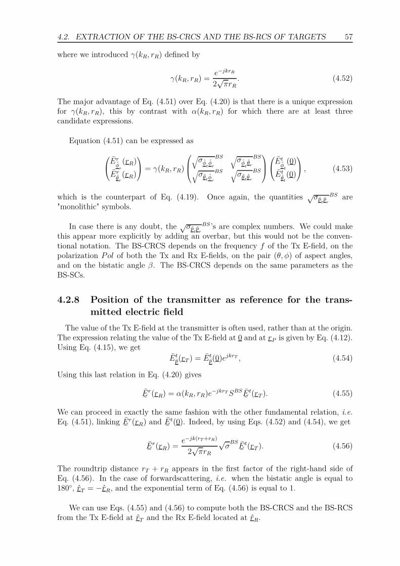
4.2. EXTRACTION OF THE BS-CRCS AND THE BS-RCS OF TARGETS 57

where we introduced γ(kR, rR) defined by

γ(kR, rR) =e−jkrR

2√πrR

. (4.52)

The major advantage of Eq. (4.51) over Eq. (4.20) is that there is a unique expressionfor γ(kR, rR), this by contrast with α(kR, rR) for which there are at least threecandidate expressions.

Equation (4.51) can be expressed as

Erφ

r

(rR)

Erθr

(rR)

= γ(kR, rR)

√σφ

tφ

r

BS √σφ

tθr

BS

√σθtφr

BS √σθtθr

BS

Etφ

t

(0)

Etθt

(0)

, (4.53)

which is the counterpart of Eq. (4.19). Once again, the quantities √σptp

r

BS are"monolithic" symbols.

In case there is any doubt, the √σptp

r

BS ’s are complex numbers. We could makethis appear more explicitly by adding an overbar, but this would not be the conven-tional notation. The BS-CRCS depends on the frequency f of the Tx E-field, on thepolarization Pol of both the Tx and Rx E-fields, on the pair (θ, φ) of aspect angles,and on the bistatic angle β. The BS-CRCS depends on the same parameters as theBS-SCs.

4.2.8 Position of the transmitter as reference for the trans-

mitted electric field

The value of the Tx E-field at the transmitter is often used, rather than at the origin.The expression relating the value of the Tx E-field at 0 and at rP is given by Eq. (4.12).Using Eq. (4.15), we get

Etp(rT ) = Et

p(0)ejkrT , (4.54)

Using this last relation in Eq. (4.20) gives

E˜r(rR) = α(kR, rR)e−jkrTSBSE

˜t(rT ). (4.55)

We can proceed in exactly the same fashion with the other fundamental relation, i.e.Eq. (4.51), linking E

˜r(rR) and E

˜t(0). Indeed, by using Eqs. (4.52) and (4.54), we get

E˜r(rR) =

e−jk(rT +rR)

2√πrR

√σBSE˜t(rT ). (4.56)

The roundtrip distance rT + rR appears in the first factor of the right-hand side ofEq. (4.56). In the case of forwardscattering, i.e. when the bistatic angle is equal to180◦, rT = −rR, and the exponential term of Eq. (4.56) is equal to 1.

We can use Eqs. (4.55) and (4.56) to compute both the BS-CRCS and the BS-RCSfrom the Tx E-field at rT and the Rx E-field located at rR.

58 4.2. EXTRACTION OF THE BS-CRCS AND THE BS-RCS OF TARGETS

4.2.9 Case of a single linear polarization

Let us consider the case of a single linear polarization, meaning that the Tx E-fieldis polarized along some (physical) direction p, and that we sense only the componentof the Rx E-field along the same direction p. For simplicity, we consider here only thecases of horizontal polarization (p = φ) and of vertical polarization (p = θ).

If we transmit along φ and we receive along φ, it should be clear that the only partof interest that remains from Eq. (4.56) is

Erφ(rR) =

e−jk(rT +rR)

2√πrR

√σφφE

tφ(rT ). (4.57)

If we transmit along θ and we receive along θ, the corresponding relation is

Erθ(rR) =

e−jk(rT +rR)

2√πrR

√σθθE

tθ(rT ). (4.58)

If the polarization is not considered, all the subscripts can be dropped, which resultsin

Er(rR) = α′(k, rT , rR)√σEt(rT ), (4.59)

where

α′(k, rT , rR) =e−jk(rT +rR)

2√πrR

. (4.60)

Equation (4.59) will be used in Chapter 5 for the construction of images of targetsfrom their BS-CRCS.

From Eq. (4.59), we can express the BS-CRCS√σ as

√σ =

1α′(k, rT , rR)

Er(rR)Et(rT )

(4.61)

= 2√πrRe

jk(rT +rR) Er(rR)

Et(rT ), (4.62)

which is exactly the definition of the BS-CRCS given by Eq. (3.1).

Similarly, we can express the BS-RCS σ as

σ = 4πr2R

|Er(rR)|2|Et(rT )|2

, (4.63)

which is, not surprisingly, exactly the definition of the BS-RCS expressed in Eq. (3.2).We can thus express both the BS-CRCS and the BS-RCS of a target in function of thetransmitted and received electric fields, provided that we know the distances rT andrR.

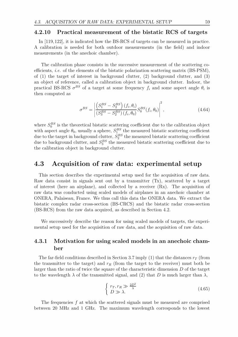
4.3. ACQUISITION OF RAW DATA: EXPERIMENTAL SETUP 59

4.2.10 Practical measurement of the bistatic RCS of targets

In [119,122], it is indicated how the BS-RCS of targets can be measured in practice.A calibration is needed for both outdoor measurements (in the field) and indoormeasurements (in the anechoic chamber).

The calibration phase consists in the successive measurement of the scattering co-efficients, i.e. of the elements of the bistatic polarization scattering matrix (BS-PSM),of (1) the target of interest in background clutter, (2) background clutter, and (3)an object of reference, called a calibration object in background clutter. Indoor, thepractical BS-RCS σBS of a target at some frequency fi and some aspect angle θi isthen computed as

σBS =

∣∣∣∣∣∣

(SBS1 − SBS2

)(fi, θi)

(SBS3 − SBS2 ) (fi, θ0)SBS0 (fi, θ0)

∣∣∣∣∣∣

2

, (4.64)

where SBS0 is the theoretical bistatic scattering coefficient due to the calibration objectwith aspect angle θ0, usually a sphere, SBS1 the measured bistatic scattering coefficientdue to the target in background clutter, SBS2 the measured bistatic scattering coefficientdue to background clutter, and SBS3 the measured bistatic scattering coefficient due tothe calibration object in background clutter.

4.3 Acquisition of raw data: experimental setup

This section describes the experimental setup used for the acquisition of raw data.Raw data consist in signals sent out by a transmitter (Tx), scattered by a targetof interest (here an airplane), and collected by a receiver (Rx). The acquisition ofraw data was conducted using scaled models of airplanes in an anechoic chamber atONERA, Palaiseau, France. We thus call this data the ONERA data. We extract thebistatic complex radar cross-section (BS-CRCS) and the bistatic radar cross-section(BS-RCS) from the raw data acquired, as described in Section 4.2.

We successively describe the reason for using scaled models of targets, the experi-mental setup used for the acquisition of raw data, and the acquisition of raw data.

4.3.1 Motivation for using scaled models in an anechoic cham-

ber

The far-field conditions described in Section 3.7 imply (1) that the distances rT (fromthe transmitter to the target) and rR (from the target to the receiver) must both belarger than the ratio of twice the square of the characteristic dimension D of the targetto the wavelength λ of the transmitted signal, and (2) that D is much larger than λ,

{rT , rR ≫ 2D2

λ

D ≫ λ.(4.65)

The frequencies f at which the scattered signals must be measured are comprisedbetween 20 MHz and 1 GHz. The maximum wavelength corresponds to the lowest

60 4.3. ACQUISITION OF RAW DATA: EXPERIMENTAL SETUP

frequency (since λ = c/f). More specifically, for the minimum frequency of 20 MHz,the corresponding wavelength is 15 m. This is the maximum wavelength we musthandle. We will see in Section 4.3.4 that the characteristic dimension D of the targetsof interest is 15 m. Therefore, according to the far-field conditions in Eq. (4.65), rTand rR must be both larger than 30 m. Since the anechoic chamber at ONERA cannothandle such ranges, one must resort to using scale models of the targets of interest.

Since we use scale models, we measure the BS-CRCS√σ of targets at a frequency

f ′ different from the desired frequency f . The frequency f ′ is equal to the productof the desired frequency f and the scale factor s, f ′ = f × s. A scale factor s of 10means that the scale model of an object is 10 times smaller than the real-size object.This ensures that the contribution of the scale model illuminated at frequency f ′ tothe echo-path signal is the same as would be the contribution of the real-size targetilluminated at frequency f . This homothety is applicable since scale models are madeof perfectly conducting materials.

To obtain the full-scale BS-CRCS at frequency f , one can show that one must simplymultiply by the scale factor the BS-CRCS obtained from the BS-CRCS measured onthe scale model [104]:

√σ(full scale, f) =

√σ(scale s, f ′) × s. (4.66)

As a consequence of the definitions of the BS-CRCS and the BS-RCS, we have [104]

σ(full scale, f) = σ(scale s, f ′) × s2. (4.67)

4.3.2 Configuration geometry

Figure 4.4 shows the configuration geometry. The origin of the coordinate system islocated at the turntable, in the center of the anechoic chamber. The target of interestS, also called the object, is fixed and placed on the turntable, and thus at the originO of the coordinate system. The transmitter (Tx) is fixed, and located on the x-axis,at a distance rT from the origin O. The receiver (Rx) can move along one-half of thecircumference of a circle, in the xy-plane, in order to make the bistatic angle β vary.The distance rT from the transmitter to the object is kept constant and equal to thedistance rR from the object to the receiver. Thus, rT = rR = r.

We define the orientation of the object as the angle between the line-of-sight ofthis object and the x-axis. The orientation of the object is defined in terms of both itsazimuth angle θ and its elevation angle φ (Fig. 4.4). The azimuth angle θ is the anglemeasured positively from the x-axis to the projection of the longitudinal axis of theairplane in the (x, y) plane. The elevation angle φ is the angle measured positivelyfrom the x-axis to the projection of the longitudinal axis of the airplane in the (y, z)plane.

In the configuration described above, the airplane and the Tx are fixed. The Rxmoves, thus making the bistatic angle β vary. The rotation of the receiver around thefixed airplane is equivalent to the rotation, in the opposite direction, of the airplanewith a fixed receiver. Experiments are thus conducted as if airplanes were rotating.

4.3. ACQUISITION OF RAW DATA: EXPERIMENTAL SETUP 61

b

b

θ

rT

rR

S = O

Moving Rx

Stationary Tx x

y

Line-of-Sight

β

z

φ

Figure 4.4: Experimental setup used to collect raw data in an anechoic chamber.

In real-life situations, although airplanes can fly arbitrary trajectories, they gener-ally fly according to a linear trajectory, at least locally. In a linear trajectory, for afixed transmitter and a fixed receiver, the bistatic angle β varies with the translationof the airplane, as shown in Fig. 4.5. Figure 4.6 illustrates the variation of the bistaticangle β along a real-life airplane trajectory, as will be seen in Chapter 8. Therefore,the rotation of the receiver in the anechoic chamber corresponds to the translation ofan airplane along its trajectory.

u

u

b

b

b

b

b

b

b

b

b

b

β1

Tx

Rx

βi

βN P1

Pi

PNAirplane trajectory

Figure 4.5: Illustration of the variation of the bistatic angle β for an airplane flyinga linear trajectory.

4.3.3 Acquisition of raw data

In the anechoic chamber, at a particular time instant, the Tx sends out a signal ata particular carrier frequency f and at a particular polarization Polt, where t standsfor "transmitter". The signal is scattered by a target with a fixed orientation, i.e. withfixed angles θ and φ. The Rx is at a fixed location. The bistatic angle β is thusfixed. The Rx collects the scattered signal at a particular polarization Polr, where

62 4.3. ACQUISITION OF RAW DATA: EXPERIMENTAL SETUP

0 5 10 15 20 25 30 35 40 45 5030

40

50

60

70

80

90

100

110

120

130Bistatic angle β as a function of time

Time index

Bis

tatic

ang

le β

[°]

Figure 4.6: Example evolution of the bistatic angle β through time, for an A319airplane flying a real trajectory, probably close to linear.

the subscript r stands for "receiver". The values used for the azimuth angle θ andthe elevation angle φ of the target, for the bistatic angle β, for the polarizations Poltand Polr, and for the frequency f are listed below. As explained in Chapter 3, theseparameters all influence the value of both the BS-CRCS and the BS-RCS.

Orientation of the target

The orientation of the target is determined by both its azimuth angle θ and its eleva-tion angle φ. Data was recorded for the following values of θ and φ: θ ∈ {0◦, 45◦, 90◦}and φ ∈ {−10◦, 0◦, 5◦}.

Frequencies

Our goal is to use frequencies from 20 MHz to 1.3 GHz. Note that these are thereal-life frequencies of interest, and that these must be scaled for use with the scalemodels. The above frequency range is covered with the four following frequency bands:FB1 ([20; 80] MHz), FB2 ([190; 250] MHz), FB3 ([450; 550] MHz), and FB4 ([1.2; 1.3]GHz). These are the four frequency bands for which raw data was acquired. We useseveral frequencies within each band, spaced by 0.1 MHz for FB1, and by 1 MHz forthe three others.

Bistatic angles

Since we only consider the bistatic RCS region (Section 3.7.4), we kept the bistaticangle β in the range from 5◦ to 180◦. More specifically, we kept the bistatic anglebetween 6◦ and 160◦, so that β ∈ [0◦; 180◦]. The increment in β was varied accordingto the frequency band used: ∆β = 2◦ for FB1, ∆β = 1◦ for FB2, ∆β = 0.5◦ for FB3,and ∆β = 0.25◦ for FB4.

4.3. ACQUISITION OF RAW DATA: EXPERIMENTAL SETUP 63

Polarizations

The polarizations of the Tx and the Rx are generally denoted by the pair Polt Polr.For linear polarizations, i.e. horizontal (H) and vertical (V ) polarizations, the possiblepolarization pairs are HH,HV, V H, V V . For circular polarizations, i.e. left (L) andright (R) polarizations, the possible polarization pairs are LL,LR,RL,RR. In ourexperiments, we used the linear polarizations only.

4.3.4 Airplanes of interest

The four airplanes considered for the experiments in the anechoic chamber are aSuper King Air 200 (Beechcraft), an F117 stealth fighter (F-117), an F16 fighter, anda Learjet. These airplanes are illustrated in Figs. 4.7, 4.8, 4.9, and 4.10, respectively.The illustrating views were generated from Computer-Aided Design (CAD) models.

In order to constitute the different classes of targets, it is useful to examine thedifferences in shape and sizes among these four airplanes. They all have a length of 15meters, and wingspans of about 10 meters. They thus do not differ in size. However,they present major differences in shape. The Beechcraft is made of a rounded fuselageand has two propeller engines located on the wings. It also has a horizontal stabilizerat its rear. The F117 is made of numerous planar facets in order to defeat radar. TheF16 is made of a rounded fuselage, two triangular wings, a rudder, and a sharp nose.It also has two missiles at the wingtips. The Learjet is similar to the Beechcraft, butwith jet engines located directly on the fuselage, and above the wings. It also has onefuel tank at each wingtip.

Figure 4.7: Perspective view of a Beechcraft produced from a three-dimensional CADmodel [210].

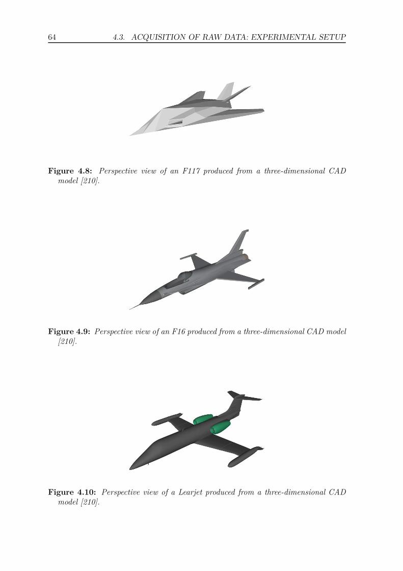
64 4.3. ACQUISITION OF RAW DATA: EXPERIMENTAL SETUP

Figure 4.8: Perspective view of an F117 produced from a three-dimensional CADmodel [210].

Figure 4.9: Perspective view of an F16 produced from a three-dimensional CAD model[210].

Figure 4.10: Perspective view of a Learjet produced from a three-dimensional CADmodel [210].

4.4. SCATTERING REGIONS 65

4.4 Scattering regions for the frequency bands of

interest

We saw in Section 3.6 that the scattering mechanisms, and thus the scatteringregions, are functions of the ratio λ/D, where λ = c/f is the illuminating wavelength,and D the characteristic dimension of the airplane. Table 4.1 gives, for each frequencyband of interest, the ratio λ/D for the two frequencies at the edges of the band forD = 15 m, which is the characteristic dimension of all airplanes of interest. Thisallows one to determine the scattering region for each of the bands. These are shownat the bottom of the columns. Note that the scattering region for FB2 is mostly optical.

Freq.band

FB1 FB2 FB3 FB4

Freq.limits

F1Min

20MHzF1Max

80MHzF2Min

190MHzF2Max

250MHzF3Min

450MHzF3Max

550MHzF4Min

1.2GHzF4Max

1.3GHz

λ (m) 15 3.75 1.5 1.2 0.66 0.55 0.25 m 0.2

λ/D 1 0.25 0.1 0.08 0.044 0.0367 0.0167 0.0133

Scatt.region

Resonance Resonance/optical Optical Optical

Table 4.1: Determination of the scattering region for each frequency band, accordingto the ratio λ/D, with D = 15 m.

We saw in Section 3.6 that the geometric parameter that most affects the scatteringin each of the three scattering regions are the following:

• Rayleigh region: volume,

• Resonance region: volume and shape,

• Optical region: shape.

Since the scattering mechanisms at work for FB1 are those of the resonance region, weconclude that the measured values of both the BS-CRCS and the BS-RCS for this bandwill be more a function of the volume than of the shape. Since the volumes of the fourairplanes are similar, one cannot expect high classification rates for the first frequencyband. Since the scattering mechanisms at work for FB2, FB3, and FB4 are those ofthe optical region, we conclude that the measured values of both the BS-CRCS andthe BS-RCS will be more a function of the shape than of the volume for these threebands.

4.5 Classes of airplanes

The conclusion just reached above indicates that it makes a lot of sense to defineas many classes of airplanes as there are significantly different shapes of airplanes ofinterest. As a result, the four airplanes of interest, here Beechcraft, F117, F16, andLearjet, certainly deserve their own individual class.

66 4.6. ILLUSTRATION OF THE BS-CRCS AND THE BS-RCS OF TARGETS

4.6 Illustration of the bistatic complex and real

RCS of targets

We now show examples of the squared magnitude and phase of the bistatic complexradar cross-section (BS-CRCS)

√σ for the different targets of interest. The squared

magnitude of the BS-CRCS is equal to the bistatic radar cross-section (BS-RCS), asdiscussed in Chapter 3. We illustrate the variation of both the squared magnitudeand the phase of the BS-CRCS as a function of the different parameters that havean influence on the BS-CRCS, i.e. the bistatic angle, the frequency, the polarizationsof both the transmitter and the receiver, and the orientation (in both azimuth andelevation) of the target. We also show how the squared magnitude and phase of theBS-CRCS vary according to the type of target. We will see that the four airplanes ofinterest exhibit differences.

As indicated in Section 4.3, we acquired the BS-CRCS√σ for four airplanes, over

four different frequency bands, four polarization pairs, and for bistatic angles varyingfrom 6◦ to 160◦, all this for three different azimuth angles θ and three different elevationangles φ. For confidentiality reasons, the maximum value of the squared magnitude ofthe BS-CRCS is not reported, but the graphs are normalized according to a commonreference for all airplanes, so that it is possible to compare the squared magnitudesand the phase of the BS-CRCS of different airplanes. The squared magnitudes aredisplayed on a logarithmic scale, and the phase is always reduced to the interval [0, 2π[.

For conciseness, we do not show the total amount of data acquired. We simplyshow the variations of both the squared magnitude and the phase of the BS-RCSfor one parameter at a time. Figure 4.11 is used as the reference for the compar-ison of the variation of the BS-CRCS as a function of the different parameters.The figure shows the squared magnitude and the phase of the BS-CRCS of aBeechcraft at an azimuth angle θ = 0◦ and an elevation angle φ = −10◦. We showthe values of the BS-CRCS for FB2, i.e. for frequencies ranging from 190 MHz to250 MHz, for the HH polarization pair, and for bistatic angles ranging from 6◦ to 160◦.

4.6.1 Variation of the bistatic complex RCS as a function ofthe bistatic angle

Figure. 4.12 shows the variation of both the squared magnitude (in dBs) and thephase of the BS-CRCS as a function of the bistatic angle β for each of the fourairplanes of interest at the center frequency of FB1, i.e. 50 MHz. Figures 4.13, 4.14,and 4.15 show the corresponding graphs for the three other frequency bands, i.e. FB2to FB4.

For a particular frequency, the variations of both the squared magnitude and thephase of the BS-CRCS as a function of β do not seem to be particular. Therefore,we do not a priori favor any bistatic angle for the recognition of the four airplanes ofinterest.

4.6. ILLUSTRATION OF THE BS-CRCS AND THE BS-RCS OF TARGETS 67

Frequency [Hz]

Bis

tatic

Ang

le [°

]

Squared magnitude of CRCS of Beechcraft, for frequency band 2 and polarization HH

1.9 2 2.1 2.2 2.3 2.4 2.5

x 108

20

40

60

80

100

120

140

160 −100

−90

−80

−70

−60

−50

−40

−30

−20

−10

0

Frequency [Hz]

Bis

tatic

Ang

le [°

]

Phase of CRCS of Beechcraft, for frequency band 2 and polarization HH

1.9 2 2.1 2.2 2.3 2.4 2.5

x 108

20

40

60

80

100

120

140

160 0

1

2

3

4

5

6

Figure 4.11: Squared magnitude (left) and phase (right) of the BS-CRCSs of aBeechcraft as a function of the frequency f and bistatic angle β, for FB2 (f ∈[190; 250] MHz), and for the following fixed parameters: Pol = HH, θ = 0◦, andφ = −10◦.

0 20 40 60 80 100 120 140 160−35

−30

−25

−20

−15

−10

−5

0

Bistatic angle [°]

Squ

ared

mag

nitu

de [d

B]

Squared magnitude of CRCS of airplanes as a function of β, for frequency = 50 MHz

BeechcraftF117F16Learjet

0 20 40 60 80 100 120 140 160−4

−3

−2

−1

0

1

2

3

4

Bistatic angle [°]

Pha

se o

f CR

CS

[rad

]

Phase of CRCS of airplanes as a function of β, for frequency = 50 MHz

BeechcraftF117F16Learjet

Figure 4.12: Squared magnitude (left) and phase (right) of the BS-CRCSs as a func-tion of β for each of the four airplanes of interest, for the following fixed parameters:f = 50 MHz (in FB1), Pol = HH, θ = 0◦, and φ = −10◦.

68 4.6. ILLUSTRATION OF THE BS-CRCS AND THE BS-RCS OF TARGETS

0 20 40 60 80 100 120 140 160−35

−30

−25

−20

−15

−10

−5

0

Bistatic angle [°]

Squ

ared

mag

nitu

de [d

B]

Squared magnitude of CRCS of airplanes as a function of β, for frequency = 220 MHz

BeechcraftF117F16Learjet

0 20 40 60 80 100 120 140 160−4

−3

−2

−1

0

1

2

3

4

Bistatic angle [°]P

hase

of C

RC

S [r

ad]

Phase of CRCS of airplanes as a function of β, for frequency = 220 MHz

BeechcraftF117F16Learjet

Figure 4.13: Squared magnitude (left) and phase (right) of the BS-CRCSs as a func-tion of β for each of the four airplanes of interest, for the following fixed parameters:f = 220 MHz (in FB2), Pol = HH, θ = 0◦, and φ = −10◦.

0 20 40 60 80 100 120 140 160−50

−45

−40

−35

−30

−25

−20

−15

−10

−5

0

Bistatic angle [°]

Squ

ared

mag

nitu

de [d

B]

Squared magnitude of CRCS of airplanes as a function of β, for frequency = 500 MHz

BeechcraftF117F16Learjet

0 20 40 60 80 100 120 140 160−4

−3

−2

−1

0

1

2

3

4

Bistatic angle [°]

Pha

se o

f CR

CS

[rad

]

Phase of CRCS of airplanes as a function of β, for frequency = 500 MHz

BeechcraftF117F16Learjet

Figure 4.14: Squared magnitude (left) and phase (right) of the BS-CRCSs as a func-tion of β for each of the four airplanes of interest, for the following fixed parameters:f = 500 MHz (in FB3), Pol = HH, θ = 0◦, and φ = −10◦.

4.6. ILLUSTRATION OF THE BS-CRCS AND THE BS-RCS OF TARGETS 69

0 20 40 60 80 100 120 140 160−60

−50

−40

−30

−20

−10

0

Bistatic angle [°]

Squ

ared

mag

nitu

de [d

B]

Squared magnitude of CRCS of airplanes as a function of β, for frequency = 1.25 GHz

BeechcraftF117F16Learjet

0 20 40 60 80 100 120 140 160−4

−3

−2

−1

0

1

2

3

4

Bistatic angle [°]

Pha

se o

f CR

CS

[rad

]

Phase of CRCS of airplanes as a function of β, for frequency = 1.25 GHz

BeechcraftF117F16Learjet

Figure 4.15: Squared magnitude (left) and phase (right) of the BS-CRCSs as a func-tion of β for each of the four airplanes of interest, for the following fixed parameters:f = 1.25 GHz (in FB4), Pol = HH, θ = 0◦, and φ = −10◦.

4.6.2 Variation of the bistatic complex RCS as a function ofthe frequency

We illustrate here the variations of the squared magnitude and the phase of theBS-CRCS as a function of the frequency, for the four airplanes of interest. Figure 4.11already illustrated the variations of both the squared magnitude and the phase of theBS-CRCS of the Beechcraft as a function of frequency, for FB2. Figures 4.16, 4.17,and 4.18 illustrate the variations of both the squared magnitude and the phase ofthe BS-CRCS of the same Beechcraft for the three other frequency bands. Althoughwe do not show the variations of both the squared magnitude and the phase of theBS-CRCS for the three other airplanes (F16, F117, and Learjet), their variations aresimilar, and the conclusions drawn for the Beechcraft apply to the three other airplanes.

More specifically, it can be seen in Figs. 4.11, 4.16, 4.17, and 4.18 that the numberof oscillations of the phase of the BS-CRCS as a function of the bistatic angle (overthe range β = [6◦; 160◦]), at a particular frequency, is approximately equal to theratio of the characteristic dimension D = 15 m of the target to the wavelength λ.For example, at a frequency of 220 MHz, λ ≈ 1.36 m, and thus D/λ = 11, which isapproximately the number of oscillations of the phase of the BS-CRCS for each of thefour types of targets, as can be seen in Fig. 4.11. Similar observations can be madefor the other frequency bands, i.e. at 50 MHz in Fig. 4.16, at 500 MHz in Fig. 4.17,and at 1.25 GHz in Fig. 4.18.

We illustrate in Figs. 4.19, 4.20, 4.21, and 4.22 the squared magnitude and thephase of the BS-CRCS of the four targets as a function of frequency, for a bistaticangle β = 20◦, for each of the four frequency bands. The number of oscillationsof the squared magnitude of the BS-CRCS of the four airplanes increases as thefrequency increases. This is explained by the fact that the scattering mechanismsmove from the resonance region for the first frequency band, to the optical regionfor the fourth frequency band. Similar variations of the squared magnitude of the

70 4.6. ILLUSTRATION OF THE BS-CRCS AND THE BS-RCS OF TARGETS

Frequency [Hz]

Bis

tatic

Ang

le [°

]

Squared magnitude of CRCS of Beechcraft, for frequency band 1 and polarization HH

2 3 4 5 6 7 8

x 107

20

40

60

80

100

120

140

160 −100

−90

−80

−70

−60

−50

−40

−30

−20

−10

0

Frequency [Hz]B

ista

tic A

ngle

[°]

Phase of CRCS of Beechcraft, for frequency band 1 and polarization HH

2 3 4 5 6 7 8

x 107

20

40

60

80

100

120

140

160 0

1

2

3

4

5

6

Figure 4.16: Squared magnitude (left) and phase (right) of the BS-CRCSs of aBeechcraft as a function of frequency f and bistatic angle β, for FB1 (f ∈ [20; 80]MHz), and for the following fixed parameters: Pol = HH, θ = 0◦, and φ = −10◦.

Frequency [Hz]

Bis

tatic

Ang

le [°

]

Squared magnitude of CRCS of Beechcraft, for frequency band 3 and polarization HH

4.5 4.6 4.7 4.8 4.9 5 5.1 5.2 5.3 5.4 5.5

x 108

20

40

60

80

100

120

140

160 −100

−90

−80

−70

−60

−50

−40

−30

−20

−10

0

Frequency [Hz]

Bis

tatic

Ang

le [°

]

Phase of CRCS of Beechcraft, for frequency band 3 and polarization HH

4.5 4.6 4.7 4.8 4.9 5 5.1 5.2 5.3 5.4 5.5

x 108

20

40

60

80

100

120

140

160 0

1

2

3

4

5

6

Figure 4.17: Squared magnitude (left) and phase (right) of the BS-CRCSs of aBeechcraft as a function of frequency f and bistatic angle β, for FB3 (f ∈ [450; 550]MHz), and for the following fixed parameters: Pol = HH, θ = 0◦, and φ = −10◦.

4.6. ILLUSTRATION OF THE BS-CRCS AND THE BS-RCS OF TARGETS 71

Frequency [Hz]

Bis

tatic

Ang

le [°

]

Squared magnitude of CRCS of Beechcraft, for frequency band 4 and polarization HH

1.2 1.21 1.22 1.23 1.24 1.25 1.26 1.27 1.28 1.29 1.3

x 109

20

40

60

80

100

120

140

160 −100

−90

−80

−70

−60

−50

−40

−30

−20

−10

0

Frequency [Hz]

Bis

tatic

Ang

le [°

]

Phase of CRCS of Beechcraft, for frequency band 4 and polarization HH

1.2 1.21 1.22 1.23 1.24 1.25 1.26 1.27 1.28 1.29 1.3

x 109

20

40

60

80

100

120

140

160 0

1

2

3

4

5

6

Figure 4.18: Squared magnitude (left) and phase (right) of the BS-CRCSs of aBeechcraft as a function of frequency f and bistatic angle β, for FB4 (f ∈ [1.2; 1.30]GHz), and for the following fixed parameters: Pol = HH, θ = 0◦, and φ = −10◦.

BS-CRCS occur at the other available bistatic angles, but we do not discuss them here.

2 3 4 5 6 7 8

x 107

−35

−30

−25

−20

−15

−10

−5

0

frequency [Hz]

Squ

ared

mag

nitu

de [d

B]

Squared magnitude of CRCS of airplanes as a function of frequency, for β = 20°

BeechcraftF117F16Learjet

2 3 4 5 6 7 8

x 107

−4

−3

−2

−1

0

1

2

3

4

frequency [Hz]

Pha

se o

f CR

CS

[rad

]

Phase of CRCS of airplanes as a function of frequency, for β = 20°

BeechcraftF117F16Learjet

Figure 4.19: Squared magnitude (left) and phase (right) of the BS-CRCSs as a func-tion of the frequency f for each of the four airplanes of interest, for FB1 (f ∈ [20; 80]MHz), and for the following fixed parameters: β = 20◦, Pol = HH, θ = 0◦, andφ = −10◦.

For a particular bistatic angle, the variations of both the squared magnitude andthe phase of the BS-CRCS as a function of the frequency f do not seem to be partic-ular. Therefore, we do not a priori favor any frequency for the recognition of the fourairplanes of interest.

72 4.6. ILLUSTRATION OF THE BS-CRCS AND THE BS-RCS OF TARGETS

1.9 2 2.1 2.2 2.3 2.4 2.5

x 108

−20

−18

−16

−14

−12

−10

−8

−6

−4

−2

0

frequency [Hz]

Squ

ared

mag

nitu

de [d

B]

Squared magnitude of CRCS of airplanes as a function of frequency, for β = 20°

BeechcraftF117F16Learjet

1.9 2 2.1 2.2 2.3 2.4 2.5

x 108

−4

−3

−2

−1

0

1

2

3

4

frequency [Hz]

Pha

se o

f CR

CS

[rad

]

Phase of CRCS of airplanes as a function of frequency, for β = 20°

BeechcraftF117F16Learjet

Figure 4.20: Squared magnitude (left) and phase (right) of the BS-CRCSs as afunction of the frequency f for each of the four airplanes of interest, for FB2(f ∈ [190; 250] MHz), and for the following fixed parameters: β = 20◦, Pol = HH,θ = 0◦, and φ = −10◦.

4.5 4.6 4.7 4.8 4.9 5 5.1 5.2 5.3 5.4 5.5

x 108

−30

−25

−20

−15

−10

−5

0

frequency [Hz]

Squ

ared

mag

nitu

de [d

B]

Squared magnitude of CRCS of airplanes as a function of frequency, for β = 20°

BeechcraftF117F16Learjet

4.5 4.6 4.7 4.8 4.9 5 5.1 5.2 5.3 5.4 5.5

x 108

−4

−3

−2

−1

0

1

2

3

4

frequency [Hz]

Pha

se o

f CR

CS

[rad

]

Phase of CRCS of airplanes as a function of frequency, for β = 20°

BeechcraftF117F16Learjet

Figure 4.21: Squared magnitude (left) and phase (right) of the BS-CRCSs as afunction of the frequency f for each of the four airplanes of interest, for FB3(f ∈ [450; 550] MHz), and for the following fixed parameters: β = 20◦, Pol = HH,θ = 0◦, and φ = −10◦.

4.6. ILLUSTRATION OF THE BS-CRCS AND THE BS-RCS OF TARGETS 73

1.2 1.21 1.22 1.23 1.24 1.25 1.26 1.27 1.28 1.29 1.3

x 109

−18

−16

−14

−12

−10

−8

−6

−4

−2

0

frequency [Hz]

Squ

ared

mag

nitu

de [d

B]

Squared magnitude of CRCS of airplanes as a function of frequency, for β = 20°

BeechcraftF117F16Learjet

1.2 1.21 1.22 1.23 1.24 1.25 1.26 1.27 1.28 1.29 1.3

x 109

−4

−3

−2

−1

0

1

2

3

4

frequency [Hz]

Pha

se o

f CR

CS

[rad

]

Phase of CRCS of airplanes as a function of frequency, for β = 20°

BeechcraftF117F16Learjet

Figure 4.22: Squared magnitude (left) and phase (right) of the BS-CRCSs as afunction of the frequency f for each of the four airplanes of interest, for FB4(f ∈ [1.2; 1.3] GHz), and for the following fixed parameters: β = 20◦, Pol = HH,θ = 0◦, and φ = −10◦.

4.6.3 Variation of the bistatic complex RCS as a function ofthe polarization

We illustrate here the variations of both the squared magnitude and the phase of theBS-CRCS as a function of the polarization, for the Beechcraft, for each polarizationpair, i.e. HH,HV, V H , and V V , in Figs. 4.11, 4.23, 4.24, and 4.25, respectively.One must notice, as expected, that both the squared magnitude and the phase of theBS-CRCS obtained for the cross-polarizations V H and HV are not equal, since weare in a bistatic configuration, while they would be equal in a monostatic configuration.

Although we do not show the variations of both the squared magnitude and thephase of the BS-CRCS for the three other airplanes (F16, F117, and Learjet), theirvariations are similar, and the conclusions drawn for the Beechcraft apply to the threeother airplanes.

Since the variations of the squared magnitude and the phase of the BS-CRCS aresimilar from one polarization to the other, we do not a priori favor any particularpolarization for the recognition of the four airplanes of interest.

4.6.4 Variation of the bistatic complex RCS as a function of

the orientation

We illustrate here the variations of both the squared magnitude and the phase of theBS-CRCS as a function of the orientation of the airplane, for the Beechcraft. We con-sider different orientation pairs (θ, φ) : (0◦,−10◦), (45◦,−10◦), (90◦,−10◦), (0◦,−5◦),and (0◦, 0◦) in Figs. 4.11, 4.26, 4.27, 4.28, and 4.29, respectively.

Since the variations of the squared magnitude and the phase of the BS-CRCS aresimilar from one orientation pair to the other, we do not a priori favor any particular

74 4.6. ILLUSTRATION OF THE BS-CRCS AND THE BS-RCS OF TARGETS

Frequency [Hz]

Bis

tatic

Ang

le [°

]

Squared magnitude of CRCS of Beechcraft, for frequency band 2 and polarization HV

1.9 2 2.1 2.2 2.3 2.4 2.5

x 108

20

40

60

80

100

120

140

160 −100

−90

−80

−70

−60

−50

−40

−30

−20

−10

0

Frequency [Hz]B

ista

tic A

ngle

[°]

Phase of CRCS of Beechcraft, for frequency band 2 and polarization HV

1.9 2 2.1 2.2 2.3 2.4 2.5

x 108

20

40

60

80

100

120

140

160 0

1

2

3

4

5

6

Figure 4.23: Squared magnitude (left) and phase (right) of the BS-CRCSs of aBeechcraft as a function of the frequency f and bistatic angle β, for HV polar-ization, and for the following fixed parameters: f ∈ [190; 250] MHz, θ = 0◦, andφ = −10◦.

Frequency [Hz]

Bis

tatic

Ang

le [°

]

Squared magnitude of CRCS of Beechcraft, for frequency band 2 and polarization VH

1.9 2 2.1 2.2 2.3 2.4 2.5

x 108

20

40

60

80

100

120

140

160 −100

−90

−80

−70

−60

−50

−40

−30

−20

−10

0

Frequency [Hz]

Bis

tatic

Ang

le [°

]

Phase of CRCS of Beechcraft, for frequency band 2 and polarization VH

1.9 2 2.1 2.2 2.3 2.4 2.5

x 108

20

40

60

80

100

120

140

160 0

1

2

3

4

5

6

Figure 4.24: Squared magnitude (left) and phase (right) of the BS-CRCSs of aBeechcraft as a function of the frequency f and bistatic angle β, for V H polar-ization, and for the following fixed parameters: f ∈ [190; 250] MHz, θ = 0◦, andφ = −10◦.

4.6. ILLUSTRATION OF THE BS-CRCS AND THE BS-RCS OF TARGETS 75

Frequency [Hz]

Bis

tatic

Ang

le [°

]

Squared magnitude of CRCS of Beechcraft, for frequency band 2 and polarization VV

1.9 2 2.1 2.2 2.3 2.4 2.5

x 108

20

40

60

80

100

120

140

160 −100

−90

−80

−70

−60

−50

−40

−30

−20

−10

0

Frequency [Hz]

Bis

tatic

Ang

le [°

]

Phase of CRCS of Beechcraft, for frequency band 2 and polarization VV

1.9 2 2.1 2.2 2.3 2.4 2.5

x 108

20

40

60

80

100

120

140

160 0

1

2

3

4

5

6

Figure 4.25: Squared magnitude (left) and phase (right) of the BS-CRCSs of aBeechcraft as a function of the frequency f and bistatic angle β, for V V polar-ization, and for the following fixed parameters: f ∈ [190; 250] MHz, θ = 0◦, andφ = −10◦.

orientation for the recognition of the four airplanes of interest.

Frequency [Hz]

Bis

tatic

Ang

le [°

]

Squared magnitude of CRCS of Beechcraft, for frequency band 2 and polarization HH

1.9 2 2.1 2.2 2.3 2.4 2.5

x 108

20

40

60

80

100

120

140

160 −100

−90

−80

−70

−60

−50

−40

−30

−20

−10

0

Frequency [Hz]

Bis

tatic

Ang

le [°

]

Phase of CRCS of Beechcraft, for frequency band 2 and polarization HH

1.9 2 2.1 2.2 2.3 2.4 2.5

x 108

20

40

60

80

100

120

140

160 0

1

2

3

4

5

6

Figure 4.26: Squared magnitude (left) and phase (right) of the BS-CRCSs of aBeechcraft as a function of the frequency f and bistatic angle β, for θ = 45◦

and φ = −10◦, and for the following fixed parameters: f ∈ [190; 250] MHz, andPol = HH.

4.6.5 Conclusions about the variations of the bistatic com-

plex RCS as a function of the bistatic angle, frequency,polarizations, and orientation

The above sections confirmed, based on real data, that both the squared magnitudeand the phase of the BS-CRCS vary with the bistatic angle, the frequency, thepolarizations of the Tx and the Rx, the azimuth angle, and the elevation angle. In

76 4.6. ILLUSTRATION OF THE BS-CRCS AND THE BS-RCS OF TARGETS

Frequency [Hz]

Bis

tatic

Ang

le [°

]

Squared magnitude of CRCS of Beechcraft, for frequency band 2 and polarization HH

1.9 2 2.1 2.2 2.3 2.4 2.5

x 108

20

40

60

80

100

120

140

160 −100

−90

−80

−70

−60

−50

−40

−30

−20

−10

0

Frequency [Hz]B

ista

tic A

ngle

[°]

Phase of CRCS of Beechcraft, for frequency band 2 and polarization HH

1.9 2 2.1 2.2 2.3 2.4 2.5

x 108

20

40

60

80

100

120

140

160 0

1

2

3

4

5

6

Figure 4.27: Squared magnitude (left) and phase (right) of the BS-CRCSs of aBeechcraft as a function of the frequency f and bistatic angle β, for θ = 90◦

and φ = −10◦, and for the following fixed parameters: f ∈ [190; 250] MHz, andPol = HH.

Frequency [Hz]

Bis

tatic

Ang

le [°

]

Squared magnitude of CRCS of Beechcraft, for frequency band 2 and polarization HH

1.9 2 2.1 2.2 2.3 2.4 2.5

x 108

20

40

60

80

100

120

140

160 −100

−90

−80

−70

−60

−50

−40

−30

−20

−10

0

Frequency [Hz]

Bis

tatic

Ang

le [°

]

Phase of CRCS of Beechcraft, for frequency band 2 and polarization HH

1.9 2 2.1 2.2 2.3 2.4 2.5

x 108

20

40

60

80

100

120

140

160 0

1

2

3

4

5

6

Figure 4.28: Squared magnitude (left) and phase (right) of the BS-CRCSs of aBeechcraft as a function of the frequency f and bistatic angle β, for θ = 0◦

and φ = −5◦, and for the following fixed parameters: f ∈ [190; 250] MHz, andPol = HH.

4.7. CONCLUSION 77

Frequency [Hz]

Bis

tatic

Ang

le [°

]

Squared magnitude of CRCS of Beechcraft, for frequency band 2 and polarization HH

1.9 2 2.1 2.2 2.3 2.4 2.5

x 108

20

40

60

80

100

120

140

160 −100

−90

−80

−70

−60

−50

−40

−30

−20

−10

0

Frequency [Hz]

Bis

tatic

Ang

le [°

]

Phase of CRCS of Beechcraft, for frequency band 2 and polarization HH

1.9 2 2.1 2.2 2.3 2.4 2.5

x 108

20

40

60

80

100

120

140

160 0

1

2

3

4

5

6

Figure 4.29: Squared magnitude (left) and phase (right) of the BS-CRCSs of aBeechcraft as a function of the frequency f and bistatic angle β, for θ = 0◦ andφ = 0◦, and for the following fixed parameters: f ∈ [190; 250] MHz, and Pol = HH.

particular, we illustrated the fact that the scattering mechanisms occur in differentscattering regions according to the frequency band. We also illustrated the fact thatthe oscillation rate of both the squared magnitude and the phase of the BS-CRCSvary according to the ratio D/λ. This will influence the classification rate. Indeed, ifboth the squared magnitude and the phase of the BS-CRCS are similar for each of thefour airplanes of interest (Beechcraft, F117, F16, and Learjet), the recognition rate isexpected to be smaller than if they vary significantly.

According to the examples shown, we cannot a priori consider that a particularbistatic angle, a particular frequency band, a particular polarization, or a particularorientation would be preferable for the recognition of the four airplanes of interest.This observation will be confirmed by the achieved classification rates (Chapter 6).

4.7 Conclusion

The first step of each of the first two automatic target recognition (ATR) systemsis the extraction of either the bistatic complex radar cross-section (BS-CRCS) or thebistatic radar cross-section (BS-RCS) of targets. In this chapter, we presented thecomputation of both the BS-CRCS and the BS-RCS of a generic object from thetransmitted electric field and the received electric field, the latter being the raw dataused at input of each of the first two ATR systems.

We presented the experimental setup used to acquire the raw data in an anechoicchamber. In particular, we explained the reasons for using scale models of the airplanesof interest. We also presented the geometry of the setup, and the parameters used forthe acquisition of raw data, which are four frequency bands ranging from 20 MHz to1.3 GHz, the four polarization pairs HH , HV , V H , and V V , the bistatic angles ofinterest, i.e. from 6◦ to 160◦, the azimuth angle that is equal to either 0◦, 45◦, or 90◦,and the elevation angle that is equal to either 0◦, 5◦, or −10◦. We also described the

78 4.7. CONCLUSION

four airplanes of interest, i.e. a Beechcraft, an F117 stealth fighter, an F16 fighter,and a Learjet.

We determined the scattering region which the scattering mechanisms occur in, foreach frequency band. We also determined that the scattering is more influenced bythe shapes of the airplanes than by their volumes, except for the first frequency band.This made us consider each type of airplane as one class.

We illustrated the variations of both the squared magnitude and the phase of theBS-CRCS of the four airplanes of interest as a function of the bistatic angle, thefrequency, the polarization, the azimuth angle, and the elevation angle. According tothe examples shown, it seems that no particular bistatic angle, no particular frequency,no particular polarization, no particular azimuth angle, and no particular elevationangle seem to be a priori preferable for the recognition of the four airplanes of interest.

Chapter 5

Construction of radar images

Contents5.1 Motivation . . . . . . . . . . . . . . . . . . . . . . . . . . . . 79

5.2 Review of tomographic imaging . . . . . . . . . . . . . . . . 80

5.2.1 The Radon Transform . . . . . . . . . . . . . . . . . . . . . . 80

5.2.2 The 2DFT and its rotation property . . . . . . . . . . . . . . 80

5.2.3 The projection-slice theorem . . . . . . . . . . . . . . . . . . 82

5.3 Principles of monostatic radar imaging . . . . . . . . . . . 84

5.3.1 Monostatic (MS) configuration . . . . . . . . . . . . . . . . . 84

5.3.2 Monostatic (MS) radar imaging . . . . . . . . . . . . . . . . . 84

5.4 Principles of bistatic radar imaging . . . . . . . . . . . . . 87

5.4.1 Bistatic (BS) configuration . . . . . . . . . . . . . . . . . . . 87

5.4.2 Bistatic (BS) imaging . . . . . . . . . . . . . . . . . . . . . . 88

5.5 Practical construction of bistatic radar images . . . . . . . 90

5.6 Examples of constructed radar images . . . . . . . . . . . . 94

5.7 Conclusion . . . . . . . . . . . . . . . . . . . . . . . . . . . . 97

Section 5.1 states the motivation for the construction of radar images of the airplanesof interest. Section 5.2 reviews some fundamental principles used in tomographic imag-ing. Sections 5.3 and 5.4 describe the principles of radar imaging for a monostatic con-figuration and a bistatic configuration, respectively. Section 5.5 presents the practicalconstruction of radar images of objects from the bistatic complex radar cross-sections(BS-CRCSs) of these objects. Section 5.6 shows examples of constructed radar imagesof the airplanes of interest. Section 5.7 concludes.

5.1 Motivation for the construction of radar images

of targets

Our first automatic target recognition system (ATR), the block diagram of which isshown in Fig. 5.1, recognizes targets by using their radar images. We discuss, in this

79

80 5.2. REVIEW OF TOMOGRAPHIC IMAGING

chapter, the second stage of this ATR system, i.e. the construction of the radar imagesof targets from the bistatic complex radar cross-section (BS-CRCS) of these targets.

Figure 5.1: Block diagram of our ATR system using radar images of targets.

5.2 Review of tomographic imaging

We derive the expression for the radar image of an object in terms of the complexradar cross-sections of this object by following the principles of tomographic imaging.In this section, we review three fundamental principles that are used in tomographicimaging, which are the Radon Transform (RT), the Fourier Transform (FT), and theprojection-slice theorem (PST). We also review the rotation property of the FT.

5.2.1 The Radon Transform

Figure 5.2 illustrates the Radon Transform (RT) [24,97,138,139,167]. Let us consideran object characterized by its two-dimensional (2D) density distribution f(x, y). Wedenote the projection of f(x, y) on a line x′ at orientation φ by pφ(x′). We have

pφ(x′) =

∫

l(x′)f(x, y) dy′, (5.1)

where l(x′) is any line orthogonal to line x′. pφ(x′) is also called a line integral [97].

The RT of f(x, y), denoted by Rf(x′, φ), is defined as the projection of f(x, y) forany orientation φ. We define it mathematically as [24, 97, 138, 139,167]

Rf(x′, φ) =∫ +∞

−∞

∫ +∞

−∞f(x, y)δ(x cosφ+ y sin φ− x′) dxdy, (5.2)

where δ is the Dirac delta function, and the coordinates x, y, x′, and φ are defined inFig. 5.2.

5.2.2 The two-dimensional Fourier Transform and its rotation

property

We define the one-dimensional (1D) FT F (ω) of a function f(x) as [24, 142]

F (ω) = f(ω) =∫ +∞

−∞f(x)e−jωx dx, (5.3)

5.2. REVIEW OF TOMOGRAPHIC IMAGING 81

f(x, y)

x

y

x′

φ

x′y′

p φ(x

′ )

l(x′)

b

O

Figure 5.2: Illustration of the Radon Transform. The projection of f(x, y) on a linex′ at orientation φ is denoted by pφ(x

′).

where ω is the pulsation. We define the inverse FT as

f(x) =1

2π

∫ +∞

−∞F (ω)ejωx dω. (5.4)

We similarly define the 2D FT F (ωx, ωy) of a function f(x, y) as [24, 142]

F (ωx, ωy) = f(ωx, ωy) =∫ +∞

−∞

∫ +∞

−∞f(x, y)e−jπ(ωxx+ωyy) dxdy. (5.5)

The 2D inverse FT is defined as

f(x, y) =1

(2π)2

∫ +∞

−∞

∫ +∞

−∞F (ωx, ωy)e

−jπ(ωxx+ωyy) dωxdωy. (5.6)

In polar coordinates, the function f(x, y) is expressed as fp(r, θ), where the subscriptp stands for "polar", and r and θ are the polar coordinates, with x = r cos θ andy = r sin θ, as shown in Fig. 5.3. The 2D FT Fp(ρ, φ) of a function fp(r, θ) is definedas

Fp(ρ, φ) =∫ +∞

0

∫ 2π

0fp(r, θ)e

−j2πρr cos(φ−θ)r dθdr, (5.7)

where ωx = ρ cosφ, and ωy = ρ sin φ.

Observe that we use two possible notations for the FT of a function f , i.e. eitherF or f (Fig. 5.3). Our preferred notation is F , but it is sometimes easier to use f .

The rotation theorem of the 2D FT, defined in [24], states that if a function fp(r, θ)undergoes a rotation of angle α, so does its 2D FT, as illustrated in Fig. 5.4. Mathe-matically, we express it as

fp(r, θ − α)2DFT⇐⇒ Fp(ρ, φ− α). (5.8)

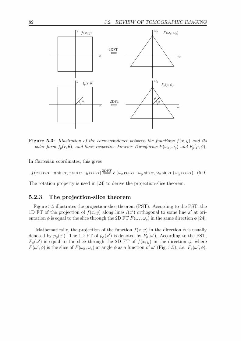
82 5.2. REVIEW OF TOMOGRAPHIC IMAGING

f(x, y)

x

y

fp(r, θ)

x

y

b

rθ

F (ωx, ωy)

ωx

Fp(ρ, φ)

bρφ

⇐⇒

⇐⇒

2DFT

2DFTωx

ωy

ωy

Figure 5.3: Illustration of the correspondence between the functions f(x, y) and itspolar form fp(r, θ), and their respective Fourier Transforms F (ωx, ωy) and Fp(ρ, φ).

In Cartesian coordinates, this gives

f(x cosα−y sinα, x sinα+y cosα)2DFT⇐⇒ F (ωx cosα−ωy sinα, ωx sinα+ωy cosα). (5.9)

The rotation property is used in [24] to derive the projection-slice theorem.

5.2.3 The projection-slice theorem

Figure 5.5 illustrates the projection-slice theorem (PST). According to the PST, the1D FT of the projection of f(x, y) along lines l(x′) orthogonal to some line x′ at ori-entation φ is equal to the slice through the 2D FT F (ωx, ωy) in the same direction φ [24].

Mathematically, the projection of the function f(x, y) in the direction φ is usuallydenoted by pφ(x′). The 1D FT of pφ(x′) is denoted by Pφ(ω′). According to the PST,Pφ(ω

′) is equal to the slice through the 2D FT of f(x, y) in the direction φ, whereF (ω′, φ) is the slice of F (ωx, ωy) at angle φ as a function of ω′ (Fig. 5.5), i.e. Fp(ω

′, φ).

5.2. REVIEW OF TOMOGRAPHIC IMAGING 83

x

y

gp(r, θ) = fp(r, θ − α)

x

y

α

ωx

Gp(ρ, φ) = fp(ρ, φ− α)

⇐⇒

⇐⇒

2DFT

2DFT

fp(r, θ) Fp(ρ, φ)

αωx

ωy

ωy

Figure 5.4: Illustration of the rotation theorem of the 2D Fourier Transform. If afunction fp(r, θ) is rotated by an angle α, then being denoted by gp(r, θ), so does itsFourier Transform Fp(ρ, φ), then being denoted by Gp(ρ, φ).

f(x, y)

x

y

x′

Fp(ω′, φ)

ωx

ωy

ω′

⇐⇒

⇐⇒

2DFT

1DFT

φ

x′

y′

φ

pφ(x′) Pφ(ω

′)

ω′

Figure 5.5: Illustration of the projection-slice theorem. The 1D FT of the projectionpφ(x

′) of f(x, y) is equal to the slice of the 2D FT Fp(ω′, φ) of f(x, y) at orientation

φ.

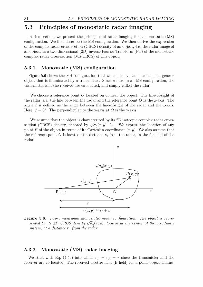
84 5.3. PRINCIPLES OF MONOSTATIC RADAR IMAGING

5.3 Principles of monostatic radar imaging

In this section, we present the principles of radar imaging for a monostatic (MS)configuration. We first describe the MS configuration. We then derive the expressionof the complex radar cross-section (CRCS) density of an object, i.e. the radar image ofan object, as a two-dimensional (2D) inverse Fourier Transform (FT) of the monostaticcomplex radar cross-section (MS-CRCS) of this object.

5.3.1 Monostatic (MS) configuration

Figure 5.6 shows the MS configuration that we consider. Let us consider a genericobject that is illuminated by a transmitter. Since we are in an MS configuration, thetransmitter and the receiver are co-located, and simply called the radar.

We choose a reference point O located on or near the object. The line-of-sight ofthe radar, i.e. the line between the radar and the reference point O is the x-axis. Theangle φ is defined as the angle between the line-of-sight of the radar and the x-axis.Here, φ = 0◦. The perpendicular to the x-axis at O is the y-axis.

We assume that the object is characterized by its 2D isotropic complex radar cross-section (CRCS) density, denoted by

√σ0(x, y) [24]. We express the location of any

point P of the object in terms of its Cartesian coordinates (x, y). We also assume thatthe reference point O is located at a distance r0 from the radar, in the far-field of theradar.

b

b

r(x, y)

O

P (x, y)

Radar x

y

r(x, y) ≈ r0 + x

r0

√σ0(x, y)

Figure 5.6: Two-dimensional monostatic radar configuration. The object is repre-sented by its 2D CRCS density

√σ0(x, y), located at the center of the coordinate

system, at a distance r0 from the radar.

5.3.2 Monostatic (MS) radar imaging

We start with Eq. (4.59) into which rT = rR = r since the transmitter and thereceiver are co-located. The received electric field (E-field) for a point object charac-

5.3. PRINCIPLES OF MONOSTATIC RADAR IMAGING 85

terized by√σ is thus expressed as

Er(r) = α′(k, r)√σEt(r), (5.10)

where

α′(k, r) =e−2jkr

2√πr, (5.11)

and Er(r) is the received electric field (E-field), Et(r) the transmitted E-field, and kthe wavenumber.

For N point objects, each object being characterized by√σi, the received E-field

is given by

Er(r) =N∑

i=1

α′(k, ri)√σiE

t(ri), (5.12)

For a patch dxdy, located at P (x, y), of an object described by its CRCS density√σ0(x, y) (Fig. 5.6), the differential phasor received is, according to Eq. (5.10),

dEr(r) = α′(k, r(x, y))√σ0(x, y)Et(r)dxdy. (5.13)

For a distributed object, the full Rx E-field is obtained by "summing" the differentialphasors dEr(r) over all patches,

Er(r) =∫ +∞

−∞

∫ +∞

−∞α′(k, r(x, y))

√σ0(x, y)Et(r)dxdy

=(∫ +∞

−∞

∫ +∞

−∞α′(k, r(x, y))

√σ0(x, y)dxdy

)Et(r). (5.14)

We express the distance r(x, y) in α′ in terms of the distance r0 and the coordinates(x, y) of the patch dxdy. The following small-angle approximation is made, for thequantity r(x, y) (Fig. 5.6),

r(x, y) =√

(r0 + x)2 + y2

= (r0 + x)

√

1 +(

y

r0 + x

)2

≈ r0 + x, (5.15)

which is intuitively true by simple inspection of Fig. 5.6. This allows us to rewriteEq. (5.11) as

α′(k, r(x, y)) =e−2jkr(x,y)

2√πr(x, y)

≈ e−2jk(r0+x)

2√π(r0 + x)

. (5.16)

Since we assume a far-field condition, we have x ≪ r0. We can thus write

α′(k, r(x, y)) ≈ e−2jk(r0+x)

2√πr0

. (5.17)

86 5.3. PRINCIPLES OF MONOSTATIC RADAR IMAGING

By substituting Eq. (5.17) into Eq. (5.14), we have

Er(r) =

(e−2jkr0

2√πr0

∫ +∞

−∞

∫ +∞

−∞e−2jkx

√σ0(x, y)dxdy

)Et(r)

=

(e−2jkr0

2√πr0

∫ +∞

−∞

(∫ +∞

−∞

√σ0(x, y)dy

)e−2jkxdx

)Et(r). (5.18)

The inner integral∫+∞

−∞√σ0(x, y)dy is the projection of

√σ0 along the y-axis. Ac-

cording to the definition of the Radon Transform (RT) introduced in Section 5.2.1, theinner integral is the RT for an angle φ = 0◦. We thus denote the above integral byR√

σ0(x′, φ). Since φ = 0◦, x′ = x, and we can write

R√σ0(x, 0) =

∫ +∞

−∞

√σ0(x, y)dy. (5.19)

Equation (5.18) thus becomes

Er(r) =e−2jkr0

2√πr0

(∫ +∞

−∞R

√σ0(x, 0)e−2jkxdx

)Et(r). (5.20)

The remaining integral has the form of a 1D FT, defined by Eq (5.3). We can thuswrite ∫ +∞

−∞R

√σ0(x, 0)e−2jkxdx = R

√σ0(2k, 0). (5.21)

We can then rewrite Eq. (5.20) as

Er(r) =e−2jkr0

2√πr0

R√σ0(2k, 0)Et(r). (5.22)

We usefully interpret Eq. (5.22) as follows. First, Er(r) is the fixed phasor of thetotal E-field received at the radar when the object is illuminated with Et(r). Second,Eq. (5.22) is exactly of the same form as the fundamental Eq. (5.10). By comparing

these two equations, one can see that R√σ0(2k, 0) can be interpreted as the monostatic

complex radar cross-section (MS-CRCS) corresponding to the entire object, i.e. to theentire distribution

√σ0(x, y). Since the object is illuminated at an angle φ of zero, we

denote this MS-CRCS by√σ(k, 0). We can thus write

√σ(k, 0) = R

√σ0(2k, 0), (5.23)

which is a remarkable result since it links the CRCS density√σ0(x, y) of the object

to the overall MS-CRCS√σ of this object.

By expanding the right-hand side of Eq. (5.23), the explicit relation between theMS-CRCS and the 2D CRCS density

√σ0(x, y) in the (x, y) coordinates is

√σ(k, 0) =

∫ +∞

−∞

(∫ +∞

−∞

√σ0(x, y)dy

)e−2jkxdx. (5.24)

We use the projection slice-theorem (PST) introduced in Section 5.2.3 to generalizeEq. (5.24) for any orientation φ. We thus have

√σ(k, φ) =

∫ +∞

−∞

∫ +∞

−∞

√σ0(x, y)e−2jk(x cosφ+y sinφ)dxdy. (5.25)

5.4. PRINCIPLES OF BISTATIC RADAR IMAGING 87

Equation (5.25) expresses the MS-CRCS√σ(k, φ) of an object as a function of the 2D

density of the MS-CRCS in the spatial domain√σ0(x, y).

By using the following change of variables

ωx = 2k cosφ

ωy = 2k sin φ,

Eq. (5.25) takes the form of a 2D FT, as defined by Eq. (5.5). By inverting the 2DFT, and performing the inverse change of variables, we get

√σ0(x, y) =

1

(2π)2

∫ +∞

0

∫ 2π

0

√σ(k, φ)e2jk(x cosφ+y sinφ)|4k|dφdk. (5.26)

Since it is usual to use the frequency f instead of the wavenumber k, with k = 2π/λ =2πf/c., we can write

√σ0(x, y) =

∫ +∞

0

∫ 2π

0

√σ

′(f, φ)e4πj f

c(x cos φ+y sinφ)|4f

c2|dφdf, (5.27)

where√σ

′(f, φ) is the MS-CRCS expressed in terms of the frequency f and the angle

φ. Equation (5.27) links the 2D CRCS density of an object to the MS-CRCS of thisobject computed at a frequency f , for an orientation φ of the radar.

5.4 Principles of bistatic radar imaging

In this section, we extend the principles of radar imaging to a bistatic (BS) config-uration. We first describe the BS configuration. We then derive the expression of theradar image, i.e. the 2D CRCS density, of an object as an inverse two-dimensional(2D) Fourier Transform (FT) of the bistatic complex radar cross-section (BS-CRCS)of this object.

5.4.1 Bistatic (BS) configuration

Figure 5.7 shows the BS configuration that we consider. Let us consider a genericobject that is illuminated by a transmitter. Since we are in an BS configuration, thetransmitter Tx and the receiver Rx are not co-located.

We choose a reference point O located on or near the object. We denote by lT theline-of-sight of the Tx, and by lR the line-of-sight of the Rx. The bistatic angle β isthe angle between the Tx and the Rx with vertex at the center of the object. The linebetween the bisector Bis of the bistatic angle and the reference point O is the x-axis.The angle φ is defined as the angle between the bisector Bis and the x-axis. Here,φ = 0◦. The perpendicular to the x-axis at O is the y-axis.

We assume that the object is characterized by its 2D isotropic complex radar cross-section (CRCS) density, denoted by

√σ0(x, y) [24]. We express the location of any

point P of the object in terms of either its Cartesian coordinates (x, y) or its polarcoordinates (r, θ). We denote by rT and rR the distances from the transmitter Tx andthe receiver Rx to the point P , respectively. We also assume that the reference pointO is located at a distance r0 from both the Tx and the Rx, in the far-field of both theTx and the Rx.

88 5.4. PRINCIPLES OF BISTATIC RADAR IMAGING

b

b

rR(x, y)

O

P (r, θ)

Tx

x

y

√σ0(x, y)

Rx

rT (x, y)

β

b

Bis

β/2

lR

lTr0

r0

Figure 5.7: Two-dimensional bistatic radar configuration. The object is representedby its 2D complex radar cross-section density

√σ0(x, y), located at the center of the

coordinate system, at a distance r0 from the Tx and the Rx.

5.4.2 Bistatic (BS) imaging

In the monostatic (MS) configuration, we consider the projection of√σ0(x, y) in the

direction of φ, which is the direction of the radar. The line integrals are perpendicularto the line-of-sight of the radar.

In the bistatic (BS) configuration, we define the bistatic distance as the sum of thedistance from the reference point O on the object to the Tx and the distance from thereference point O on the object to the Rx. The bistatic distance remains equal whenthe object moves along an ellipse whose foci are the Tx and the Rx [224]. The reflexivityproperty of ellipses tells us that, at any point on the ellipse, the tangent of the ellipse,and thus the line integrals, are perpendicular to the bisector of the bistatic angle [224],as shown in Fig. 5.8. Therefore, we can consider a BS configuration as an MS configu-ration, with the radar being located on the bisector of the bistatic angle, at a distancethat is half of the sum of the distances from the Tx and the Rx to the reference point O.

If we can express the bistatic distance rT + rR in terms of 2r0 +X, we can considerEq. (5.24), into which we replace the MS roundtrip distance 2x by X. We thus needto compute the distances rT and rR.

Without loss of generality, we assume the distances from the Tx and the Rx tothe center of coordinates to be equal to r0. By inspection of Fig. 5.7, we express the

5.4. PRINCIPLES OF BISTATIC RADAR IMAGING 89

b

b b

O x

y x′

y′

β/2β/2

Tx Rx

Bis

Object

Figure 5.8: Illustration of the reflexivity property of the ellipse with the Tx and theRx located at its foci. The line integral are perpendicular to the bisector Bis of thebistatic angle.

distance rT as

rT =√

(r0 + r cos(β/2 − θ))2 + (r sin(β/2 − θ))2

=√r2

0 + 2rr0 cos(β/2 − θ) + r2

= r0

√

1 + 2r

r0

cos(β/2 − θ) +r2

r20

≈ r0

√1 + 2

r

r0cos(β/2 − θ)

≈ r0 + r cos(β/2 − θ), (5.28)

where the second to last line is obtained by considering the far-field approximation(r ≪ r0), and the last line by performing a first-order Taylor development on thesquare root.

In a similar way, we obtain the distance rR,

rR = r0 + r cos(β/2 + θ). (5.29)

We thus express the bistatic distance as

rT + rR = 2r0 + r (cos(β/2 − θ) + cos(β/2 + θ))

= 2r0 + 2r cosβ/2 cos θ

= 2r0 + 2x cos(β/2) (5.30)

We can thus substitute 2x by 2x cos(β/2) into Eq. (5.24) to get

√σBS

(k, 0) =∫ +∞

−∞

(∫ +∞

−∞

√σ0(x, y)dy

)e−2jkx cos(β/2)dx. (5.31)

90 5.5. PRACTICAL CONSTRUCTION OF BISTATIC RADAR IMAGES

where the superscript "BS" stands for the bistatic configuration.

We use the PST introduced in Section 5.2.3 to generalize Eq. (5.31) for any orien-tation φ of the bisector as

√σBS

(k, φ) =∫ +∞

−∞

∫ +∞

−∞

√σ0(x, y)e−2jk cos(β/2)(x cosφ+y sinφ)dxdy. (5.32)

Equation (5.32) expresses the BS-CRCS√σBS

(k, φ) of an object as a function of the2D CRCS density

√σ0(x, y).

By using the following change of variables

ωx = 2k cos(β/2) cosφ

ωy = 2k cos(β/2) sinφ,

Eq (5.32) takes the form of a 2D FT, as defined by Eq. (5.5). By inverting the FT,and performing the inverse change of variables, we thus get

√σ0(x, y) =

1

(2π)2

∫ +∞

0

∫ 2π

0

√σBS

(k, φ)e2jk cos(β/2)(x cos φ+y sinφ)|4k cos2(β/2)|dφdk.(5.33)

Since it is usual to use the frequency f instead of the wavenumber k, with k = 2π/λ =2πf/c, we can write

√σ0(x, y) =

∫ +∞

0

∫ 2π

0

√σ

′BS(f, φ)e4πj f

ccos(β/2)(x cosφ+y sinφ)|4f cos2(β/2)

c2|dφdf, (5.34)

where√σ

′BS(f, φ) is the BS-CRCS expressed in terms of the frequency f . Equa-

tion (5.34) links the 2D CRCS density of an object to the BS-CRCS of this objectcomputed at a frequency f , for an orientation φ of the bisector of the bistatic angle.

In the anechoic chamber that we used to extract the BS-CRCS of the airplanes ofinterest (Chapter 4), the Tx is fixed, and located on the x-axis. This corresponds to arotation of β/2 of the configuration depicted in Fig 5.7. Moreover, the object is fixed,and the Rx moves around the object. We thus integrate over the bistatic angle β ratherthan on the aspect angle φ. We thus get

√σ0(x, y) =

∫ +∞

0

∫ 2π

0

√σ

′BS(f, φ)e4πj f

ccos(β/2)(x cos(φ+β/2)+y sin(φ+β/2)|4f cos2(β/2)

c2|dβdf.(5.35)

5.5 Practical construction of bistatic radar images

As shown in Fig. 5.1, we compute the radar images of the targets of interest, i.e. the2D CRCS density

√σ0(x, y) of these targets, from the complex radar cross-sections

(CRCSs) of these targets, for a bistatic configuration. In this section, we detail thepractical construction of these radar images.

5.5. PRACTICAL CONSTRUCTION OF BISTATIC RADAR IMAGES 91

Recall from Chapter 4 that the available bistatic complex radar cross-section(BS-CRCS) is computed over four different frequency bands, four different polar-izations, and several bistatic angles, at three azimuth angles and three elevationangles, for the four airplanes of interest. For computational reasons, we decide to usethe values of the BS-CRCS that are extracted for the HH polarization only. For aparticular azimuth angle, a particular elevation angle, a particular polarization, and aparticular frequency band, the BS-CRCS of a particular target is extracted over somefrequency range and some range of bistatic angles. We can thus usefully represent theBS-CRCS as a two-dimensional array of values of BS-CRCS, the dimensions of thearray being the frequency f and the bistatic angle β, as shown in Fig. 5.9.

For recognition purposes (Chapter 6), we split the values of the BS-CRCS into alearning set (LS), and a test set (TS). For a particular frequency band, the LS containsthe values of BS-CRCS that are available over the lower half of this frequency band,and the TS contains the values of BS-CRCS that are available over the upper half ofthis frequency band. Images of targets are constructed using values of BS-CRCS thatbelong to either the LS or the TS. The constructed images thus belong to either theLS of images or the TS of images, in order to guarantee the independence of the LSand the TS in our recognition experiments [221].

βf

LS

TS

∆β

∆f

fm

fM

βm βM

BS-CRCSs selected

to contruct an image

Figure 5.9: Illustration of the practical reconstruction of an image of a target fromthe BS-CRCSs of this target.

In Section 5.4, we expressed the radar images of targets as an inverse 2D FourierTransform of the bistatic complex radar cross-section (BS-CRCS) of these targets.In particular, Eq. (5.35) states that the value of each pixel (x, y) of an image of atarget is obtained by "summing" the BS-CRCS of the target over an infinite range offrequencies, and a particular range of bistatic angles. As shown in Fig. 5.9, the valuesof BS-CRCS that are used to construct an image of a target can thus be viewed asbelonging to a sub-array of the available values of BS-CRCS. The dimensions of thissub-array are [βm; βM ] × [fm; fM ], where the subscripts "m" and "M" stand for theminimum and maximum values of each of the dimensions of the array, respectively.

92 5.5. PRACTICAL CONSTRUCTION OF BISTATIC RADAR IMAGES

We arbitrarily decide to fix the range of the bistatic angle as being comprisedbetween 20◦ and 25◦. We thus have ∆β = βM − βm ∈ [20◦; 25◦].

In order to fix the frequency range, we use the definitions of the range resolutionrBSx and of the cross-range resolution rBSy , where the superscript "BS" indicates, asabove, that we are in a bistatic configuration. For a monostatic (MS) configuration,the range resolution rMS

x and the cross-range resolution rMSy are given by [165]

rMSx =

c

2∆f(5.36)

andrMSy =

c

2fc∆θ, (5.37)

where c is the speed of light, ∆θ is the aspect angular range (in radians), and ∆fand fc are the frequency range and the central frequency of the data selected toreconstruct an image, respectively.

For a bistatic (BS) configuration, the range resolution rBSx and the cross-rangeresolution rBSy are given by [41]

rBSx =c

2∆f cosβ/2(5.38)

andrBSy =

c

fc∆β, (5.39)

where c is the speed of light, and β and ∆β are the bistatic angle and the bistaticangular range of the data selected to reconstruct an image, respectively.

Since we use the constructed images for classification, we want all the images tohave similar range resolutions and similar cross-range resolutions. In order to do so,we arbitrarily decide that we want the ratio of the range resolution and the cross-rangeresolution of an image to be almost equal to unity. We also want to construct a numberof images large enough to perform meaningful classification. We can thus express thesetwo conditions as

1

α≤ rBSxrBSy

≤ α, (5.40)

where α is experimentally chosen to comply with the two conditions stated above.Table 5.1 lists the chosen values of α, for each frequency band.

In short, for a given range of bistatic angle, and for a given frequency range, wecompute rBSx and rBSy . If Eq. (5.40) is satisfied, we construct the radar image basedon Eq. (5.35). Otherwise, we do not construct any image for the selected sub-array ofvalues of BS-CRCS. The construction process is repeated for all possible sub-arrays.

Table 5.2 shows, for each frequency band, the mean and standard deviation of therange resolution rBSx and of the cross-range resolution rBSy , for the constructed imagesof the Beechcraft from the BS-CRCSs of the LS. Similarly, Table 5.3 shows, for each

5.5. PRACTICAL CONSTRUCTION OF BISTATIC RADAR IMAGES 93

Frequency band α ∆β

FB1: 20 − 80 MHz 1.001 [20; 25]◦

FB2: 190 − 250 MHz 1.02 [20; 25]◦

FB3: 450 − 550 MHz 1.2 [20; 25]◦

FB4: 1.2 − 1.3 GHz 2.9 [20; 25]◦

Table 5.1: Experimentally chosen values of α for each frequency band.

frequency band, the mean and standard deviation of the range resolution rBSx and ofthe cross-range resolution rBSy , for the constructed images of the Beechcraft from theBS-CRCS of the TS.

rx [m] ry [m]Frequency band Mean Std. dev. Mean Std. dev.

FB1: 20 − 80 MHz 21.07 2.30 21.06 2.31FB2: 190 − 250 MHz 3.12 0.11 3.12 0.10FB3: 450 − 550 MHz 1.61 0.03 1.38 0.04FB4: 1.2 − 1.3 GHz 1.58 0.02 0.55 10−4

Table 5.2: Mean and standard deviation of the range resolution rBSx and of the cross-range resolution rBSy of the reconstructed images of the Beechcraft belonging to theLS.

rx [m] ry [m]Frequency band Mean Std. dev. Mean Std. dev.

FB1: 20 − 80 MHz 11.35 1.19 11.35 1.20FB2: 190 − 250 MHz 3.11 0.10 3.12 0.09FB3: 450 − 550 MHz 1.62 0.02 1.38 0.0024FB4: 1.2 − 1.3 GHz 1.59 10−13 0.55 10−14

Table 5.3: Mean and standard deviation of the range resolution rBSx and of the cross-range resolution rBSy of the reconstructed images of the Beechcraft belonging to theTS.

From Tables 5.2, and 5.3, we make the following observations for the Beechcraft:

• For each frequency band, and for both the LS and the TS, the means (andstandard deviation) of rBSx and rBSy are very similar. This makes sense since bothrBSx and rBSy are computed from Eq. (5.40).

• For each frequency band, the mean value of rBSx is greater for the LS than forthe TS, and the same is true for rBSy . This makes sense since the images of theLS and the TS are constructed from the lower part and the upper part of thefrequency band, respectively.

94 5.6. EXAMPLES OF CONSTRUCTED RADAR IMAGES

The same observations apply to the three other airplanes of interest, since theirBS-CRCSs are computed for the same parameters (frequency, polarization, bistaticangle, azimuth angle, and elevation angle).

Table 5.4 shows the number of constructed images of each type of airplane for boththe LS and the TS, for each frequency band. These images are used in Chapter 6 forthe recognition of the four airplanes of interest.

Frequency band Number of imagesLS TS

FB1: [20; 80] MHz 6,480 11,520FB2: [190; 250] MHz 12,600 11,340FB3: [450; 550] MHz 14,580 7,290FB4: [1.2; 1.3] GHz 14,040 4,680

Table 5.4: Number of constructed images of each type of airplanes for the LS and theTS, per frequency band.

5.6 Examples of constructed radar images

In this section, we show examples of constructed images of the four airplanesof interest. For conciseness, we choose to show images that are constructed fromtheir BS-CRCS computed only for bistatic angles ranging from 6◦ to 43.5◦, for anorientation angle θ of 0◦ and for an elevation angle φ of 0◦. The values of the frequencyand bistatic angles are chosen such that they satisfy Eq. (5.40).

Figure 5.10 shows one radar image (shown in pseudocolor for ease of visualization)for each of the four airplanes of interest. These images are constructed for the dataacquired in the first frequency band, FB1. Figures 5.11, 5.12, and 5.13 give thecorresponding images for the three other frequency bands, FB2, FB3, and FB4,respectively. The values in each image are normalized to a maximum value of 1 (0dB).

Tables 5.2 and 5.3 show that the means of rBSx and of rBSy are about 21 m, whichis slightly larger than the characteristic dimension of the airplanes, i.e. 15 m. Asa result, each target appears essentially as a single bright point (Fig. 5.10). SincerBSx and rBSy decrease when the frequency increases, targets are characterized by anincreasing number of smaller bright points when the frequency increases.

5.6. EXAMPLES OF CONSTRUCTED RADAR IMAGES 95

Cross−range [Pixel]R

ange

[Pix

el]

Sample Beech image reconstructed from its C−RCS’s [dB]

20 40 60 80 100 120 140 160 180 200

20

40

60

80

100

120

140

160

180

200 −20

−18

−16

−14

−12

−10

−8

−6

−4

−2

0

(a) Beechcraft

Cross−range [Pixel]

Ran

ge [P

ixel

]

Sample Beech image reconstructed from its C−RCS’s [dB]

20 40 60 80 100 120 140 160 180 200

20

40

60

80

100

120

140

160

180

200 −20

−18

−16

−14

−12

−10

−8

−6

−4

−2

0

(b) F117

Cross−range [Pixel]

Ran

ge [P

ixel

]

Sample Beech image reconstructed from its C−RCS’s [dB]

20 40 60 80 100 120 140 160 180 200

20

40

60

80

100

120

140

160

180

200 −20

−18

−16

−14

−12

−10

−8

−6

−4

−2

0

(c) F16

Cross−range [Pixel]

Ran

ge [P

ixel

]

Sample Beech image reconstructed from its C−RCS’s [dB]

20 40 60 80 100 120 140 160 180 200

20

40

60

80

100

120

140

160

180

200 −20

−18

−16

−14

−12

−10

−8

−6

−4

−2

0

(d) Learjet

Figure 5.10: Example radar images computed from BS-CRCSs collected over the firstfrequency band FB1 ([20; 80] MHz). The images are shown using a pseudocolor scale.

Cross−range [Pixel]

Ran

ge [P

ixel

]

Sample Beech image reconstructed from its C−RCS’s [dB]

20 40 60 80 100 120 140 160 180 200

20

40

60

80

100

120

140

160

180

200 −20

−18

−16

−14

−12

−10

−8

−6

−4

−2

0

(a) Beechcraft

Cross−range [Pixel]

Ran

ge [P

ixel

]

Sample Beech image reconstructed from its C−RCS’s [dB]

20 40 60 80 100 120 140 160 180 200

20

40

60

80

100

120

140

160

180

200 −20

−18

−16

−14

−12

−10

−8

−6

−4

−2

0

(b) F117

Cross−range [Pixel]

Ran

ge [P

ixel

]

Sample Beech image reconstructed from its C−RCS’s [dB]

20 40 60 80 100 120 140 160 180 200

20

40

60

80

100

120

140

160

180

200 −20

−18

−16

−14

−12

−10

−8

−6

−4

−2

0

(c) F16

Cross−range [Pixel]

Ran

ge [P

ixel

]

Sample Beech image reconstructed from its C−RCS’s [dB]

20 40 60 80 100 120 140 160 180 200

20

40

60

80

100

120

140

160

180

200 −20

−18

−16

−14

−12

−10

−8

−6

−4

−2

0

(d) Learjet

Figure 5.11: Example radar images computed from BS-CRCSs collected over thesecond band FB2 ([190; 250] MHz). The images are shown using a pseudocolor scale.

96 5.6. EXAMPLES OF CONSTRUCTED RADAR IMAGES

Cross−range [Pixel]

Ran

ge [P

ixel

]

Sample Beech image reconstructed from its C−RCS’s [dB]

20 40 60 80 100 120 140 160 180 200

20

40

60

80

100

120

140

160

180

200 −20

−18

−16

−14

−12

−10

−8

−6

−4

−2

0

(a) Beechcraft

Cross−range [Pixel]

Ran

ge [P

ixel

]

Sample Beech image reconstructed from its C−RCS’s [dB]

20 40 60 80 100 120 140 160 180 200

20

40

60

80

100

120

140

160

180

200 −20

−18

−16

−14

−12

−10

−8

−6

−4

−2

0

(b) F117

Cross−range [Pixel]

Ran

ge [P

ixel

]

Sample Beech image reconstructed from its C−RCS’s [dB]

20 40 60 80 100 120 140 160 180 200

20

40

60

80

100

120

140

160

180

200 −20

−18

−16

−14

−12

−10

−8

−6

−4

−2

0

(c) F16

Cross−range [Pixel]

Ran

ge [P

ixel

]

Sample Beech image reconstructed from its C−RCS’s [dB]

20 40 60 80 100 120 140 160 180 200

20

40

60

80

100

120

140

160

180

200 −20

−18

−16

−14

−12

−10

−8

−6

−4

−2

0

(d) Learjet

Figure 5.12: Example radar images computed from BS-CRCSs collected over the thirdfrequency band FB3 ([450; 550] MHz). The images are shown using a pseudocolorscale.

Cross−range [Pixel]

Ran

ge [P

ixel

]

Sample Beech image reconstructed from its C−RCS’s [dB]

20 40 60 80 100 120 140 160 180 200

20

40

60

80

100

120

140

160

180

200 −20

−18

−16

−14

−12

−10

−8

−6

−4

−2

0

(a) Beechcraft

Cross−range [Pixel]

Ran

ge [P

ixel

]

Sample Beech image reconstructed from its C−RCS’s [dB]

20 40 60 80 100 120 140 160 180 200

20

40

60

80

100

120

140

160

180

200 −20

−18

−16

−14

−12

−10

−8

−6

−4

−2

0

(b) F117

Cross−range [Pixel]

Ran

ge [P

ixel

]

Sample Beech image reconstructed from its C−RCS’s [dB]

20 40 60 80 100 120 140 160 180 200

20

40

60

80

100

120

140

160

180

200 −20

−18

−16

−14

−12

−10

−8

−6

−4

−2

0

(c) F16

Cross−range [Pixel]

Ran

ge [P

ixel

]

Sample Beech image reconstructed from its C−RCS’s [dB]

20 40 60 80 100 120 140 160 180 200

20

40

60

80

100

120

140

160

180

200 −20

−18

−16

−14

−12

−10

−8

−6

−4

−2

0

(d) Learjet

Figure 5.13: Example radar images computed from BS-CRCSs collected over thefourth frequency band FB4 ([1.2; 1.3] GHz). The images are shown using a pseudo-color scale.

5.7. CONCLUSION 97

5.7 Conclusion

We presented in this chapter the construction of radar images of targets, since thisis the second step of the first automatic target recognition (ATR) system. We derivedthe expression of the two-dimensional (2D) spatial representation of an object from thecomplex radar cross-section (CRCS) of this object for the monostatic configuration.We then extended this expression to the bistatic configuration. In both configurations,the 2D radar image of a target is basically a 2D inverse Fourier Transform of theCRCS of this target.

We then presented the practical construction of radar images from their bistaticcomplex radar cross-section (BS-CRCS), for each of the frequency bands of interest.We constructed each image from a 2D array of values of BS-CRCS of targets, whosedimensions are the bistatic angle and the frequency. The size of each dimension isdetermined such that the ratio of the range resolution and the cross-range resolutionof the obtained image is comprised between 1/α and α. For each frequency band, thevalue of α was experimentally chosen in order to obtain a number of images that islarge enough to perform a meaningful classification (as further discussed in Chapter 6).We showed, for each frequency band of interest, examples of radar images of each ofthe four airplanes of interest.

98 5.7. CONCLUSION

Chapter 6

Recognition of targetsby using their radar images

Contents6.1 Motivation . . . . . . . . . . . . . . . . . . . . . . . . . . . . 100

6.2 Physical and parameter spaces . . . . . . . . . . . . . . . . 101

6.2.1 Physical space . . . . . . . . . . . . . . . . . . . . . . . . . . 101

6.2.2 Parameter space . . . . . . . . . . . . . . . . . . . . . . . . . 105

6.3 Recognition strategy . . . . . . . . . . . . . . . . . . . . . . 106

6.4 Block diagram of the recognizer . . . . . . . . . . . . . . . 111

6.5 Production of feature vectors by window extraction . . . 112

6.6 Determination of target class model by extra-trees . . . . 113

6.6.1 Deterministic decision tree . . . . . . . . . . . . . . . . . . . 113

6.6.2 Extremely randomized trees . . . . . . . . . . . . . . . . . . . 114

6.6.3 Motivation for using extremely randomized trees . . . . . . . 115

6.7 Determination of the target class . . . . . . . . . . . . . . . 116

6.8 Quantification of performance . . . . . . . . . . . . . . . . . 116

6.9 Recognition experiments on MSTAR images . . . . . . . . 117

6.9.1 Description of MSTAR images . . . . . . . . . . . . . . . . . 117

6.9.2 Experimental sets of images . . . . . . . . . . . . . . . . . . . 117

6.9.3 Parameters of the recognizer . . . . . . . . . . . . . . . . . . 120

6.9.4 Recognition results . . . . . . . . . . . . . . . . . . . . . . . . 120

6.10 Recognition experiments on ONERA images . . . . . . . . 127

6.10.1 Experimental sets of images . . . . . . . . . . . . . . . . . . . 127

6.10.2 Parameters of the recognizer . . . . . . . . . . . . . . . . . . 128

6.10.3 Recognition results . . . . . . . . . . . . . . . . . . . . . . . . 128

6.11 Conclusion . . . . . . . . . . . . . . . . . . . . . . . . . . . . 136

99

100 6.1. MOTIVATION

In this chapter, we perform the recognition of targets by using their radar images.Section 6.1 states the motivation for the recognition of targets by using their radarimages. Section 6.2 describes the physical and the parameter spaces in which weexpress both the bistatic complex radar cross-section (BS-CRCS) and the bistatic radarcross-section (BS-RCS), and thus the images, of a target. Section 6.3 describes therecognition strategy that we use to design the recognizer. Section 6.4 describes theblock diagram of the recognizer. Section 6.5 describes the production of feature vectors.Section 6.6 describes the determination of the target class model. Section 6.7 describesthe determination of the class of an unknown target based on a target class model.Section 6.8 presents the criteria we use for the quantification of the performance of therecognizer. Sections 6.9 and 6.10 describe the recognition experiments we performedand the recognition rates we achieved on the MSTAR images and on the ONERAimages, respectively. Section 6.11 concludes.

6.1 Motivation for the recognition of targets by us-

ing their radar images

As explained in Chapter 2, the recognition of targets by using their images is oneof the most popular recognition method in automatic target recognition (ATR) forradars. Our first ATR system, whose block diagram is shown in Fig. 6.1, is designed torecognize targets by using their radar images. In this chapter, we design, implement,and test the recognition stage of this ATR system.

Figure 6.1: Block diagram of our ATR system using radar images of targets.

As explained in Chapter 5, the construction of radar images of targets from thebistatic complex radar cross-section (BS-CRCS) of these targets requires that theBS-CRCS of the targets be available over some range of frequencies and over somerange of bistatic angles. However, this two-dimensional (2D) diversity is unlikelyto be met in an operational system. Indeed, at a particular time instant and for aparticular target, it is possible to compute the BS-CRCS of this target at a particularfrequency and over a large range of bistatic angles by suitably positioning a sufficientnumber of receivers (Rx’s). The frequency diversity requires that the signals of asufficient number of transmitters (Tx’s), operating on distinct, adjacent frequencies,and covering in an adequate way a frequency band that is large enough, be scattered

6.2. PHYSICAL AND PARAMETER SPACES 101

on the target at the same time instant. However, the frequency band planning doesnot allow transmitters of opportunity to cover such a large frequency band.

Since the construction of radar images from their BS-CRCS appears difficult toperform in an operational passive bistatic radar system, we will use the recognition oftargets by using their radar images as a reference to evaluate the two subsequent ATRsystems.

6.2 Physical and parameter spaces

We showed in Chapter 3 that both the complex radar cross-section (CRCS) andthe radar cross-section (RCS) of a particular object depend on electromagnetic andgeometric parameters. Since we construct images of targets from the CRCS of thesetargets, the images also depend on the same electromagnetic and geometric parameters.The two electromagnetic parameters are the frequency and the polarization (of boththe transmitter (Tx) and the receiver (Rx)). For a monostatic (MS) configuration, thegeometric parameter is the aspect angle α, and, for a bistatic (BS) configuration, thegeometric parameters are the aspect angle α and the bistatic angle β. We refer to thisset of parameters as the parameter space.

In the present context, the objects of interest are airplanes. Airplanes fly arbitrarytrajectories that are expressed in the (x, y, z) coordinates, which we call the physicalspace. We thus need to establish the mapping between the physical space and theparameter space. We first present the physical space, and then the mapping betweenthe physical space and the parameter space. We discuss the cases of both the RCSsand the CRCSs. The discussion is similar for the images of the targets.

6.2.1 Physical space

For ease of explanation, and as is commonly done [186], we consider that thephysical space containing the Tx’s, the Rx’s, and the objects of interest (and, thus,their trajectories) is planar, i.e. 2D. Thus, we also refer to this planar physicalspace as the "physical plane". The positions of the above elements are given withrespect to some system of orthogonal (x, y) axes located in this plane. This 2D situ-ation is illustrated in Fig. 6.2. We consider a single frequency and a single polarization.

While the discussion to follow is cast into a 2D framework, it is conceptually easyto extend it to 3D. Furthermore, real-life situations where the objects of interest arelocated at sufficient distances from the Tx’s and Rx’s can generally be handled asthough they were 2D. The physical plane can then be interpreted as an overhead viewof the situation.

In this 2D framework, each object necessarily follows a continuous true trajec-tory in the physical plane (Fig. 6.2). Each (Tx,Rx) pair looks at this object atspecific discrete time instants and, thus, at specific, corresponding discrete (true)positions along its true trajectory; these positions are shown with open circles inFig. 6.2. The discrete "looks" thus result in a sampling of the true (unknown)trajectory. By analogy with the qualifiers "continuous time (CT)" and "discrete

102 6.2. PHYSICAL AND PARAMETER SPACES

x

y

bc

Tx1Trajectory

Object

bc

bc

bc

bc

bc

bc

bc

bc

bc

bc

bc

bc

ut

ut ut

ut

ut

ut

ut

ut

utut ut

ut

ut

rs

rs

rs

rs

rs

rs

rs

rs

rsrs

rs

rs

u

r

u

r

r

rs

Tx3

Tx2

Rx2

Rx1

Figure 6.2: 2D physical space, also called (x, y) plane. The figure illustrates a pas-sive radar system consisting of three transmitters Txi and two receivers Rxi, andobserving an object following a particular trajectory. The open circles on this truetrajectory indicate the true position of S at each time instant one specific (Tx,Rx)pair looks at the object. The open triangles indicate where this pair actually es-timates that the object is. The open rectangles correspond to another pair, whichwill generally provide other position estimates and, furthermore, will generally usedifferent look instants.

time (DT)" of signal processing [142], we respectively use "continuous space (CS)"and "discrete space (DS)" to qualify the continuous trajectory and the sequence ofpoints resulting from sampling. These trajectories are the domains of definition ofboth the radar-cross-section (RCS) functions and the complex radar cross-section(CRCS) functions. We can thus complete the analogy by talking about CS CRCSsignals and DS CRCS sequences, and, similarly, CS RCS signals and DS RCS sequences.

In practice, each (Tx,Rx) pair may "look" at different instants, so that, for eachobject, one must associate a specific DT trajectory (and either a corresponding DTCRCS sequence or a corresponding DT RCS sequence) to each such (Tx,Rx) pair.Furthermore, the estimates of positions for each pair will generally not fall on the truetrajectory (Fig. 6.2).

We thus distinguish between true CS, true DS, and measured DS trajectories. Thelatter two are specific to each (Tx,Rx) pair. For illustration purpose, we often showthe sampling points of a measured DS trajectory on a CS curve, but this curve ispurely conceptual.

The above trajectories are those of a reference point S on the object (Fig. 6.3),typically its center of gravity. The orientation of the object is characterized bythe orientation of a reference (unit) vector s (Fig. 6.3), typically aligned with thelongitudinal axis of the object and pointing to its front. A fundamental assumption ofour work is that we can determine (estimates of) S and s at each instant that each(Tx,Rx) pair looks at the object.

If there is no wind, s essentially coincides with the oriented tangent t to the

6.2. PHYSICAL AND PARAMETER SPACES 103

b

γ

True trajectory

ObjectS

x

y

t

s

Figure 6.3: Stylized object with reference point S on it, and reference orientationvector s through S. When the object moves, S traces the true trajectory of the objectin the (x, y) plane. Vector t is defined by the tangent to this trajectory at S and thedirection of motion of the object.

underlying true CS trajectory at S. Otherwise, there is an angle γ from t to s(Fig. 6.3). (All angles are measured counterclockwise.) While it is relatively easyto get t, perhaps following an interpolation of the measured DS trajectory, it maybe more difficult to get s. However, in one way or another, we need to know theposition S and the orientation s. If necessary, we assume that s is t. This is areasonable assumption when airplanes approach or leave a runway that is well alignedwith the wind direction. In an operational system, the positions of S are obtainedfrom either secondary surveillance radars or passive bistatic radars.

For a particular frequency f and a particular polarization Pol, both the MS-CRCS√σ and the MS-RCS σ of an object vary with the aspect angle α from the line-of-sight

(LOS) vector l to the LOS s of the object (Fig. 6.4(a)). We conceptually representthis variation by the functions

√σ(α) and σ(α). Below, we review some elementary

"geometrical" considerations for the MS-CRCS and MS-RCS [91]. We place ourselvesin a 2D configuration, i.e. we do not consider the elevation angle. This last elevationangle is thus not a parameter of the parameter space used here.

We distinguish between symmetric and asymmetric objects. This is why thestylized object used in Fig. 6.4 has an optional circular part that allows one to make itsymmetric (by omitting this part) or not. For a symmetric object, one can intuitivelydeduce from Fig. 6.4(a) that

√σ(α) and σ(α) are even in α, i.e.

√σ(α) =

√σ(−α)

and σ(α) = σ(−α). This means that, for such an object, one only needs to examinethe variations of

√σ and σ over the limited [0, π] range, instead of over the full [−π, π]

(or [0, 2π]) range, since all values of√σ(α) and σ(α) for α in [−π, 0] can be obtained

from those in [0, π]. However, this does not mean that√σ(α) and σ(α) have period π;

indeed, they have period 2π. As an aside,√σ(α) and σ(α) are generally not equal to√

σ(α+ π) and σ(α+ π), respectively. For an asymmetric object, one obviously needsto consider

√σ(α) and σ(α) over the full [−π, π] range. In conclusion, in the MS case,

we use α to parametrize the variations of both the MS-CRCS and MS-RCS.

104 6.2. PHYSICAL AND PARAMETER SPACES

b

α

LOS

T,R(a)

b

α

BIS

(b)

s

l

T R

LOSRLOST

s

b

αTαR β

lT

lR

S

bb

S

b

b b

Figure 6.4: Illustration of the aspect and bistatic angles for (a) a monostatic config-uration, and (b) a bistatic configuration.

6.2. PHYSICAL AND PARAMETER SPACES 105

The BS equivalent of the MS aspect angle α is the pair of BS aspect angles αT andαR, defined as in the MS case, but with respect to the LOS vector lT (from T ), andthe LOS vector lR (from R), respectively (Fig. 6.4(b)). Although we could use αT andαR to parametrize the variations of both the BS-CRCS

√σBS and the BS-RCS σBS ,

we use instead the bistatic angle β defined as the angle from lT to lR, and the angle αdefined as the angle from b to s, where the vector b bisects β and points towards theoutside of the triangle TSR. One can easily derive the analytical relations betweenthe pairs (αT , αR) and (α, β). This shows that one can use either pair to parametrizethe variations of both the BS-CRCS and the BS-RCS. Here, we use the pair (α, β).

When the BS configuration reduces to an MS configuration, (1) the BS vectors lT ,lR, and b coincide, and become the MS LOS vector l, (2) the BS angle α becomes theMS angle α, hence justifying the use of the same symbol α in both cases, despite thedifferent meanings, and (3) the angle β becomes zero. We use the term "aspect angle"to refer to both the MS angle α and the BS angle α.

In [188], Skolnik states that "σBS is a function of aspect angle and bistatic angle",but he does not define this aspect angle α precisely. Even though the term "bistatic(BS) angle" generally denotes the interior angle of the triangle TSR between the sidesST and SR [186], we also use this term to refer to the β introduced above (which cantake values in [0, 2π], by contrast to the usual [0, π]).

The assumed knowledge of S and of s at any specific time allows us to compute thevalues of α and β for this time. Since we assume that we know S and s at all timesof interest during an observation window, we can associate a pair (α, β) to each pointalong any trajectory. Adding

√σBS and σBS , we can associate two triplets (α, β, σBS)

and (α, β,√σBS

) to each such point.

6.2.2 Parameter space

The parameters α and β are used to define a system of orthogonal (α, β) axes anda corresponding 2D space, referred to here as the parameter plane. We also refer to itas the (α, β) space and the (α, β) plane.

For example, consider a specific measured discrete space (DS) trajectory in thephysical plane, due to one specific (Tx,Rx) pair and one specific object. For each point(x0, y0) along this trajectory, we can compute the corresponding values of α0 and β0,which define a corresponding point (α0, β0) in the (α, β) plane. Each point (x0, y0) canthus be mapped into a point (α0, β0). Since the mapping preserves the time ordering,the mapping of all the points (x0, y0) along the trajectory in the (x, y) plane results ina corresponding trajectory in the (α, β) plane. The values of both the CRCS

√σ and

the RCS σ are also carried over in the mapping. (In the case of polarimetric radars,one complex value per polarization pair would be carried over.) It is useful to visualizeone value of

√σ, or one value of σ, associated with each point on each (x, y) and

(α, β) trajectory and, thus, functions√σ(x, y) and

√σ

′(α, β), or σ(x, y) and σ′(α, β),

which are continuous space (CS) functions (using "Dirac walls" [94]) or DS sequences(using "lollipops" [33]).

106 6.3. RECOGNITION STRATEGY

The customary range of β is [0, π]; the maximum range of α is [0, π] for symmetricobjects, and [−π, π] for asymmetric objects; at a given β,

√σBS

(α) and σBS(α)

always have a period of 2π, and√σBS

(α) and σBS(α) are even for symmetric objects.However, when considering the (α, β) plane, we must always consider the full [−π, π]range of α, even for symmetric objects. Figure 6.5 shows the "central part" of the(α, β) plane, as well as two example trajectories, corresponding either to a singletrajectory observed by two (Tx,Rx) pairs, or two distinct trajectories observed by asingle pair.

Tr1

β

απ0−π

π

b

b

bb

b

b

b

b b

b

bb

b

bb

Tr2

b

b

bbbb

Figure 6.5: 2D parameter space, also called (α, β) plane. The rectangle shown is theboundary of the central part of the plane corresponding to α ∈ [−π, π] and β ∈ [0, π].Two example (α, β)-plane trajectories are shown, both in continuous form and indiscrete form. The dots on each trajectory correspond to the instants one (Tx,Rx)pair looks at the object.

We will use the parameter space, in terms of which we express both the BS-CRCSand the BS-RCS of targets, in the design of each of the three recognizers.

6.3 Recognition strategy

In this section, we define the recognition strategy that we follow for the recognitionstage (i.e. the recognizer) of each of the three automatic target recognition ATRsystems. The lifecycle of any of the recognizers starts with the laboratory development,where the recognizer is constructed and tested. It continues with the operational use.The input data are either images, bistatic complex radar cross-section (BS-CRCS), orbistatic radar cross-section (BS-RCS) of the targets of interest. We partition the datainto a learning set (LS) used for constructing the recognizer, and a test set (TS) usedfor testing it, and quantifying its performance [53, 134].

Recognition consists in assigning a "class" to data, in particular that of the TS. Insupervised learning (as assumed here), this class is one among a set of Nc predefinedclasses, each denoted here by Class ic, with ic ∈ [1, Nc].

The LS can be viewed as being organized into a set of (f, Pol, α, β) spaces, whereeach space corresponds to a predefined class, and is filled with data of this class. The

6.3. RECOGNITION STRATEGY 107

data corresponds to either images, BS-CRCS values, or BS-RCS values of the targetsof interest.

In the present context, since the polarization pair takes discrete values (HH, HV,VH, VV), we will consider each polarization independently of the others. Similarly,since the available data is computed for different non-adjacent frequency bands (FB1to FB4), we will also consider each frequency band independently of the others.Moreover, since the scattering mechanisms remain the same inside each frequencyband, we do not partition the data within a frequency band into sub-bands. Therefore,for each frequency band, and for each polarization, the LS can very advantageously beviewed as being organized into a set of (α, β) planes, where each plane corresponds toa predefined class, and is filled with data of objects of this class.

In short, for each frequency band and for each polarization, we construct onerecognizer for each of the (α, β) plane filled with data of the Nc classes. Recall thatit is sufficient to consider the central part of the (α, β) plane, which corresponds toα ∈ [−π, π] and β ∈ [0, π].

During test, one typically observes an object at a particular frequency and at aparticular polarization, over a part of the (α, β) plane. The basic ingredient for usingthe recognizer is one (α, β) plane that contains a small amount of data. Since the goalof the recognizer is to assign one of the Nc classes to the data in this (α, β) plane, it isvery advantageous to say that this plane corresponds to the unknown class, which wecall "Class x", by analogy with "Class ic". Once again, it is sufficient to consider thecentral part of this plane. The goal of the recognizer is to attribute one of the valuesic’s to x.

We now have, for each frequency band and for each polarization, a set of Nc (α, β)planes filled with data and ready to be used for constructing the recognizer, and one(α, β) plane for holding the data to be recognized, i.e. a sort of scratchpad to holddata temporarily. Figure 6.6(a) illustrates, for each frequency band and for each polar-ization, the central part of each of these planes and the measured DS data they contain.

As will soon become clear, our approach to recognition can be applied either tothe central parts of these planes, or to any common subset thereof. As illustratedin Fig. 6.7, this subset, called here "cookie-cutter region", can be of arbitrary shape.Figure 6.6(b) shows such a region overlayed on the central parts. This regionautomatically segments out the data in (the central part of) all (α, β) planes. One canthen consider only the data that is segmented out (Fig. 6.6(c)).

A key feature of our approach is that, for each frequency band and each polariza-tion, we use the data from the same region in the Nc planes to construct a recognizerspecific to this region and the Nc classes. We call the recognizer specific to a givenregion a sub-recognizer. During test, the data from the same region in the plane forClass x is presented to the (sub-)recognizer.

Instead of cutting out a single region from the (α, β) plane, we can cut outseveral regions, whether overlapping or not, and construct one recognizer for each.

108 6.3. RECOGNITION STRATEGY

β

απ0−π

π

Class1β

απ0−π

π

b

b

ClassNc

. . .

β

απ0−π

π

Classx

β

απ0−π

π

b

b

b

b

b

b

(a)

b bb

bb

bb

bb

bbb

b

b

b

b

b

β

απ0−π

π

. . .

(b)

b

b

b

b

b

b

b

b

b

b

b

b

b

b b

bb

b

b

b

bb

b

b

b

b

β

απ0−π

π

b bb

bb

b bb

bb

bb

bbb

b

b

b

bb

b

b

. . .

(c)

b bb

bb

bb

b

b bb

bb

bbb

b

b

b

bb b

bb

b

bb

b

b

b

b

b

b

b

b

b

b

b

b

b

b

bb

b

b

bb

b

b

b

bb

bb

bbb

b bb

b

b

Figure 6.6: Illustration of the use of the generic cookie-cutter region of Fig. 6.7 toextract the same corresponding region from the (α, β) plane of each class of interest,i.e. Class 1, ..., Class Nc, and Class x. The cookie-cutter region automaticallysegments out portions of the data present in the various (α, β) planes. The recognizeris built from the data so isolated for Classes 1 to Nc. The recognition is performedusing the data so isolated for Class x.

β

απ0−π

π

Cookie-cutter

Central part

region

Figure 6.7: Illustration of the (generic) cookie-cutter region. It delimits one region -consisting of one or more subregions - in the central part of the generic (α, β) plane.It is used as a cookie cutter to isolate the same region in the (α, β) planes of theclasses of interest, i.e. Class 1, ..., Class Nc, and Class x.

6.3. RECOGNITION STRATEGY 109

To handle the full central part, it is sufficient to define a collection of overlapping ornon-overlapping subsets of it. One important covering is obtained by subdividing theα and β axes into contiguous intervals, and using these intervals to define rectangulartiles (Fig. 6.8). One recognizer specific to each tile must be constructed. One canchoose regions/tiles that overlap or not.

Tr1

β

απ0−π

π

b

b

bb

b

b

b

b b

b

bb

b

bb

Tr2

b

b

bbbb

Figure 6.8: Partitioning of the central part of the (α, β) plane using an example 4 ×3array of butting, non-overlapping tiles fully covering the central part (with 4 and 3corresponding to α and β, respectively). A recognizer would be built for each tile,and recognition would be performed tile-by-tile.

One advantage of decomposing the central part into several regions is that therecognizer constructed for each tile will likely have better performance, since it mustonly deal with limited angular coverages in α and β. One disadvantage lies in thenumber of recognizers one must construct.

Figure 6.9 gives a bird’s eye view of the recognizer we build for any givenregion, such as a rectangular tile for a particular frequency band and for a par-ticular polarization. The first block diagram concerns the "construction" of thecorresponding sub-recognizer, which uses the LS data for all Nc classes to producea target class model. For each of the Nc classes, one first produces feature vectors(FVs) [134,208], and one then computes the "best" target class model from all the FVs.

The second block diagram concerns the "test" of the recognizer and its "operationaluse". In both cases, one first produces one FV (at a time) from the appropriate data forthe region of interest. One then determines the class that the (sub-)recognizer assignsto this FV by using the corresponding target class model. The difference between test(TS) and operational use (operational data) is the availability of the ground truth forthe TS, which allows one to quantify the performance of the (sub-)recognizer for theregion considered.

If enough computational power is available, one can envision adjusting the cookie-cutter region on-the-fly. This would imply recomputing the FVs and the target classmodel on-the-fly, prior to testing the new FV of interest on the target class model.

110 6.3. RECOGNITION STRATEGY

Figure 6.9: Block diagrams summarizing the generic architecture of any of the sub-recognizers of the recognition stage (i.e. the recognizer) of each of the three ATRsystems. (a) shows the successive steps in building the target class model, and (b) thesuccessive steps in performing the recognition, either for testing (and performanceevaluation) or for operational use.

6.4. BLOCK DIAGRAM OF THE RECOGNIZER 111

6.4 Block diagram of the recognizer

The input data of the recognizer are the images that we constructed from the bistaticcomplex radar cross-section (Chapter 5) of the targets of interest. The four targetsof interest are a Beechcraft, an F117 fighter, an F16 fighter, and a Learjet. Eachtype of target corresponds to a particular target class. We thus consider Nc = 4 classes.

Each image is labelled a value for each of the parameters of the parameter space,which are the frequency band f , the polarization Pol, the aspect angle α, and thebistatic angle β. As described in Section 6.3, we divide the parameter space into tiles,and we build a recognizer for each tile. As explained in Chapter 5, we constructedimages for the HH polarization only, for each of the four frequency bands, each of thethree aspect angles, and several bistatic angles ranging from 6◦ to 160◦. We arbitrarilydivide the range of bistatic angle into 12 overlapping sectors, as described in Table 6.1.We thus build 4 × 3 × 12 recognizers, one for each frequency band, and for each tile ofthe (α, β) plane.

Bistatic angular sector index Bistatic angular sector (degrees)

1 (6, 43.5)2 (18.5, 56)3 (31, 68.5)4 (43.5, 81)5 (56, 93.5)6 (68.5, 106)7 (81, 118.5)8 (93.5, 131)9 (106, 143.5)10 (118.5, 156)11 (131, 168.5)12 (143.5, 181)

Table 6.1: Bistatic angular sectors considered.

Figure 6.10 gives the block diagrams of the recognizer we build for any giventile. The first block diagram concerns the "construction" of the corresponding sub-recognizer, which uses the LS data for all Nc classes to produce a recognition "model"consisting of a list of extremely randomized trees (extra-trees). We describe thedetermination of the target class model in Section 6.6. For each of the Nc classes, onefirst produces feature vectors (FVs). Each FV consists in an ensemble of windows thatwe extract from each input image. We describe the extraction of windows in Section 6.5.

The second block diagram concerns the "test" of the sub-recognizer and its"operational use". In both cases, one first produces one FV (at a time) from theappropriate data for the tile of interest. One then propagates each FV througheach of the extra-tree, thus assigning a class to each window of the FV for eachextra-tree. A majority vote among the assigned classes determines the class that the(sub-)recognizer assigns to this FV. The difference between test (TS) and operational

112 6.5. PRODUCTION OF FEATURE VECTORS BY WINDOW EXTRACTION

Figure 6.10: Block diagrams summarizing the architecture of any of the sub-recognizers of the recognition stage. (a) shows the successive steps in building thetarget class model, and (b) the successive steps in performing the actual recognition,either for testing (and performance evaluation) or for operational use.

use (operational data) is the availability of the ground truth for the TS, which allowsone to quantify the performance of the recognizer for the tile considered.

The joint use of windows extracted from an image and of extra-trees was developedand tested by Marée for the classification/recognition of non-radar images of objects,and reported in [123, 124].

6.5 Production of feature vectors by window ex-

traction

The first step of the recognizer, for both the construction of the target class modeland the test of the target class model, consists in the production of feature vectors(FVs). Each FV consists in the pixel values inside a fixed number of windows whichwe extract out of each image. The method for the extraction of windows is reportedin [126, 129].

For each image of the learning set (LS), we extract a large number Nls of squarewindows of random sizes (constrained between α% and β% of the image size), atrandom positions. Figure 6.11 shows an example of 4 windows that are extracted outof a particular radar image. We then resize each window to a fixed, given size w × h,so that all windows are described by the same number of pixels. Each window ischaracterized by its pixel values i.e. w × h numerical values in the case of grayscale

6.6. DETERMINATION OF TARGET CLASS MODEL BY EXTRA-TREES 113

images. Each window is also assigned the class of its parent image.

Figure 6.11: Example of four windows that we extract out of a particular image.

A similar process is repeated for the construction of the FV for any image of thetest set (TS). The number of extracted windows can be different, and is denoted byNts. The locations of the windows extracted from images of the LS and for the TScan be different. The main difference is that each window is labelled, but only forquantifying the performance of the recognizer.

6.6 Determination of the target class model by

extra-trees

In this section, we present the determination of the target class model from thefeature vectors (FVs) that we extracted from the images of the learning set (LS).The target class model consists of an ensemble of extremely randomized decisiontrees (extra-trees). The first tree-based methods classified objects based on a singledeterministic decision tree [25]. Then, tree-based methods started using ensemble oftrees, called forests, to classify objects. Different methods to randomize the trees areused, such as bagging [26], random forests [27], and extra-trees [69]. A brief history ofthe different decision-trees methods appears in [124].

6.6.1 Deterministic decision tree

Before describing the concept of an extra-tree, we first briefly describe the classical(binary) deterministic decision tree. Below, we successively describe the constructionof the tree and its use for classifying previously-unseen inputs, as illustrated inFig. 6.12. A deterministic decision tree is a collection of "if-then" mutually exclusivedecision rules that recursively separate objects of the input LS into disjoint subsetsof objects, until each subset contains objects of (mainly) a single class (in case offully-developed trees). When a subset contains objects of (mainly) a single class, it iscalled a terminal node, or leaf. The links between two nodes are called branches.

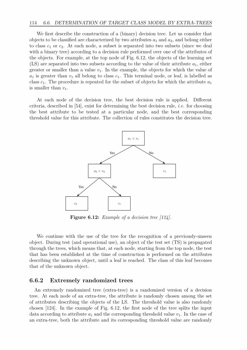
114 6.6. DETERMINATION OF TARGET CLASS MODEL BY EXTRA-TREES

We first describe the construction of a (binary) decision tree. Let us consider thatobjects to be classified are characterized by two attributes a1 and a2, and belong eitherto class c1 or c2. At each node, a subset is separated into two subsets (since we dealwith a binary tree) according to a decision rule performed over one of the attributes ofthe objects. For example, at the top node of Fig. 6.12, the objects of the learning set(LS) are separated into two subsets according to the value of their attribute a1, eithergreater or smaller than a value v1. In the example, the objects for which the value ofa1 is greater than v1 all belong to class c1. This terminal node, or leaf, is labelled asclass c1. The procedure is repeated for the subset of objects for which the attribute a1

is smaller than v1.

At each node of the decision tree, the best decision rule is applied. Differentcriteria, described in [54], exist for determining the best decision rule, i.e. for choosingthe best attribute to be tested at a particular node, and the best correspondingthreshold value for this attribute. The collection of rules constitutes the decision tree.

c1

c1c2

a1 < v1

a2 < v2

Yes No

Yes No

Figure 6.12: Example of a decision tree [124].

We continue with the use of the tree for the recognition of a previously-unseenobject. During test (and operational use), an object of the test set (TS) is propagatedthrough the trees, which means that, at each node, starting from the top node, the testthat has been established at the time of construction is performed on the attributesdescribing the unknown object, until a leaf is reached. The class of this leaf becomesthat of the unknown object.

6.6.2 Extremely randomized trees

An extremely randomized tree (extra-tree) is a randomized version of a decisiontree. At each node of an extra-tree, the attribute is randomly chosen among the setof attributes describing the objects of the LS. The threshold value is also randomlychosen [124]. In the example of Fig. 6.12, the first node of the tree splits the inputdata according to attribute a1 and the corresponding threshold value v1. In the case ofan extra-tree, both the attribute and its corresponding threshold value are randomly

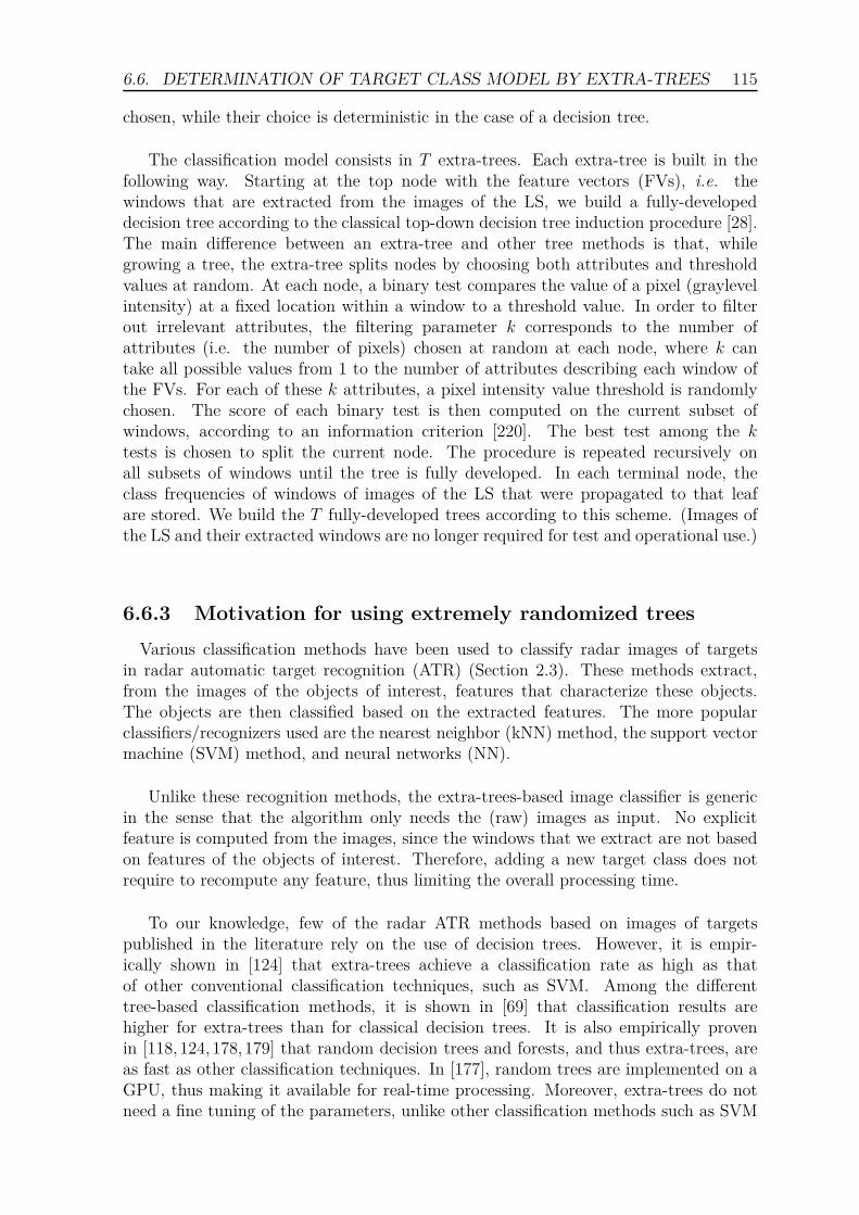
6.6. DETERMINATION OF TARGET CLASS MODEL BY EXTRA-TREES 115

chosen, while their choice is deterministic in the case of a decision tree.

The classification model consists in T extra-trees. Each extra-tree is built in thefollowing way. Starting at the top node with the feature vectors (FVs), i.e. thewindows that are extracted from the images of the LS, we build a fully-developeddecision tree according to the classical top-down decision tree induction procedure [28].The main difference between an extra-tree and other tree methods is that, whilegrowing a tree, the extra-tree splits nodes by choosing both attributes and thresholdvalues at random. At each node, a binary test compares the value of a pixel (graylevelintensity) at a fixed location within a window to a threshold value. In order to filterout irrelevant attributes, the filtering parameter k corresponds to the number ofattributes (i.e. the number of pixels) chosen at random at each node, where k cantake all possible values from 1 to the number of attributes describing each window ofthe FVs. For each of these k attributes, a pixel intensity value threshold is randomlychosen. The score of each binary test is then computed on the current subset ofwindows, according to an information criterion [220]. The best test among the ktests is chosen to split the current node. The procedure is repeated recursively onall subsets of windows until the tree is fully developed. In each terminal node, theclass frequencies of windows of images of the LS that were propagated to that leafare stored. We build the T fully-developed trees according to this scheme. (Images ofthe LS and their extracted windows are no longer required for test and operational use.)

6.6.3 Motivation for using extremely randomized trees

Various classification methods have been used to classify radar images of targetsin radar automatic target recognition (ATR) (Section 2.3). These methods extract,from the images of the objects of interest, features that characterize these objects.The objects are then classified based on the extracted features. The more popularclassifiers/recognizers used are the nearest neighbor (kNN) method, the support vectormachine (SVM) method, and neural networks (NN).

Unlike these recognition methods, the extra-trees-based image classifier is genericin the sense that the algorithm only needs the (raw) images as input. No explicitfeature is computed from the images, since the windows that we extract are not basedon features of the objects of interest. Therefore, adding a new target class does notrequire to recompute any feature, thus limiting the overall processing time.

To our knowledge, few of the radar ATR methods based on images of targetspublished in the literature rely on the use of decision trees. However, it is empir-ically shown in [124] that extra-trees achieve a classification rate as high as thatof other conventional classification techniques, such as SVM. Among the differenttree-based classification methods, it is shown in [69] that classification results arehigher for extra-trees than for classical decision trees. It is also empirically provenin [118,124,178,179] that random decision trees and forests, and thus extra-trees, areas fast as other classification techniques. In [177], random trees are implemented on aGPU, thus making it available for real-time processing. Moreover, extra-trees do notneed a fine tuning of the parameters, unlike other classification methods such as SVM

116 6.7. DETERMINATION OF THE TARGET CLASS

and NN. Extra-trees have also been successfully tested on conventional images, suchas in [146, 147].

Furthermore, it has been empirically shown in [124] that the joint use of windowsextraction and extra-trees is robust to the rotation of targets. Therefore, the jointuse of windows extraction and of an ensemble of extremely randomized decision treesappears to be a promising classification technique.

The image classifier based on the joint use of windows extraction and extra-treesdefined in [124] has been tested on numerous datasets of classical images, such asin [124, 125, 127, 128]. In order to validate the extra-trees-based method as a robustand accurate recognizer of radar images, we first test below the recognizer on thewell-known MSTAR database. We compare the achieved recognition rates with therecognition rates of other ATR systems tested on the MSTAR dataset, and publishedin the literature.

6.7 Determination of the target class

During both test and operational use, we first produce a feature vector (FV) char-acterizing the input image. The FV is a set of Nts windows from this image. We thenpropagate each window of the FV into each of the T extra-trees. The assigned classes ofall windows at terminal nodes are aggregated, and the majority class is assigned to theimage. This approach has also been extended for content-based image retrieval [130]and semantic segmentation [56].

6.8 Quantification of performance

We quantify the performance of the recognizer during the test phase, in the followingway. The primary criterion is the error rate. The error rate is defined as the ratio ofthe number of images that are wrongly classified to the total number of images thatare classified. The second criterion is the individual window error rate. The individualwindow error rate is defined as the ratio of the number of windows that are wronglyclassified to the total number of windows that are classified.

The error rate and the individual window error rate are obtained from theconfusion matrices. A confusion matrix is a two-dimensional matrix. The differenttrue classes of the objects to be classified are each represented by a row, and thedifferent classes assigned by the recognizer are each represented by a column. In theexperiments performed below, the obtained confusion matrices are square, since weforce the recognizer to assign a class to every image that we wish to classify. Eachcell (i, j) of a confusion matrix represents the number of objects of the true classi that are labelled by the computed class j. The sum of all the elements in a rowis equal to the number of objects that truly belong to the class of the row. Therecognition rate for a target class i is the ratio between the number of objects ofthat class that are truly recognized, reported in cell (i, i), to the total number ofobjects of that class. The total recognition rate is the ratio of the sum of the diagonalelements of the confusion matrix to the sum of all the elements of the confusion

6.9. RECOGNITION EXPERIMENTS ON MSTAR IMAGES 117

matrix. The total error rate is equal to one minus the total recognition rate. Forthe error rate, an object is an image of a target of interest, while, for the individualwindow error rate, an object is a window extracted from an image of a target of interest.

We choose the values of the parameters of the recognizer in order to remain com-putationally efficient. However, for two different sets of parameters, if both the errorrates and the window error rates are equal, the set of parameters for which the errorrate is achieved faster is preferred.

6.9 Recognition experiments on MSTAR images

We quantify the performance of the recognizer on images of the MSTAR data. Wefirst describe the MSTAR data, and the six different sets of images we built for therecognition experiments. We then describe the parameters of the recognizer, and therecognition results we achieve for each of the six sets of images.

6.9.1 Description of MSTAR images

The MSTAR data is a well-known database that is collected and distributed underthe DARPA Moving and Stationary Target Recognition program. The MSTARdatabase is shared by the synthetic aperture radar (SAR) ATR community. SARproduces images of targets with sufficient resolution (because of the high frequencyused, usually in the GHz) to be classified [169,171,222].

The MSTAR data consist of X-band (10 GHz) SAR images of targets. We considerthree targets of interest that are the BMP-2 and the BTR-70 armored personalcarriers (APCs), and the T-72 tank. We also consider SLICY canonical targets thatare defined in [175] as "a precisely designed and machined engineering test targetcontaining standard radar reflector primitive shapes such as flat plates, dihedrals,trihedrals, and top hats". Images of clutter, i.e. containing "things" other than thetargets of interest (BMP-2, BTR-70, T-72) and the SLICY targets, are also available.Figure 6.13 shows examples of images of each type.

Images of each of the three targets of interest were captured at two depressionangles, which are 15◦ and 17◦, over a full range of aspect angles, from 0◦ to 360◦. Eachimage is of size 128 pixels × 128 pixels. Images of the SLICY target were capturedat the depression angles of 15◦ and 30◦. The clutter images were captured at thedepression angle of 15◦.

Note that the term "clutter" is used here in the sense used by the MSTAR commu-nity, i.e. for anything that is other than the targets of interest, whether man-made ornatural.

6.9.2 Experimental sets of images

We consider the recognition of the three different targets of interest, in presence ofclutter and/or SLICY targets. Each target of interest is considered here to be a class.SLICY targets are also considered to be a class. Even though it is not possible to

118 6.9. RECOGNITION EXPERIMENTS ON MSTAR IMAGES

(a) BMP-2 APC. (b) BTR-70 APC. (c) T-72 tank.

(d) SLICY target. (e) CLUTTER. (f) CLUTTER.

Figure 6.13: Example SAR images of the various objects available in the MSTARdatabase and used for our recognition experiments.

model the clutter, we call the class representing the clutter images the non-target class.

We make up six different sets of images. We first consider the recognition of thethree targets of interest. We thus first exclusively consider images of the three targetsof interest, i.e. images of the BMP-2 APC’s, the BTR-70 APC’s, and the T-72 tanks.The first set is made up of the raw images of the three targets of interest (128 × 128pixels), as depicted in Table 6.2(a).

To get rid off the background speckle, we manually crop the raw images. Thesecond set is made up of the cropped images (Table 6.2(b)). The cropped images arethe central 64 pixels ×64 pixels of the raw images, since the target and its shadow arealways located in the central part of the raw images.

We then rotate the images of the targets, in order to get rid off the aspect angle.The third set is made up of the images of the three targets of interest that we rotateto get all the targets pointing to the same direction (Table 6.2(c)). We thus assumethat we know the orientation of the target. We perform the rotation by using theinformation provided in the header file of each image. We could use a pose estimatorto get the azimuth angle for the rotation, but rotating the target using this a prioriinformation is not necessary, as we will show in Section 6.9.4. It has also beenempirically shown in [124] that the classifier is robust to the rotation of the targets.Furthermore, we also crop the images, for the same reason as for the second set.However, since the images are rotated, we now keep the central region of 80 × 80pixels. More background speckle is present in the 80 × 80 images than in the 64 × 64images. This additional background speckle is not a problem, as we will show whenwe discuss the results (Section 6.9.4).

6.9. RECOGNITION EXPERIMENTS ON MSTAR IMAGES 119

(a)

(b)

(c)

Table 6.2: SAR images of BMP-2 targets at different aspect angles for each of thefirst three sets. (a) 128×128 raw images of the first set. (b) Cropped 64×64 imagesof the second set. (c) Cropped and rotated 80 × 80 images of the third set.

We then consider the recognition of the three targets of interest in the presence ofnon-targets (i.e. clutter). The fourth set of images is thus made up of the images ofthe three targets of interest and the non-target images.

We then consider the recognition of the three targets of interest in the presence ofSLICY targets, that act as false targets. The fifth set of images is thus made up ofthe images of the three targets of interest and the images of the SLICY targets.

Last, we consider the recognition of the three targets of interest in the presenceof both SLICY targets, that act as false targets, and non-targets (i.e. clutter). Thesixth set of images is thus made up of the images of the three targets of interest, theimages of the SLICY targets, and the non-target images.

For each of the six sets, we choose to put all the images obtained for depressionangles of 17◦ and 30◦ in the learning set (LS), and to put all the images obtained fora depression angle of 15◦ in the test set (TS). For the non-target images, since theavailable images were all taken at a depression angle of 15◦, we choose to put half ofthe images in the LS, and the other half in the TS. This partitioning of the images intoa LS and a TS is similar to the partitionings of the MSTAR images that are reportedin the literature. We are thus able to compare our results to those reported in theliterature. Table 6.3 gives, for each set, the number of images for each class, for boththe LS and the TS.

120 6.9. RECOGNITION EXPERIMENTS ON MSTAR IMAGES

BMP-2 BTR-70 T-72NON-

TARGETSSLICY Total

Set 1:LS/TS

698/587 233/196 463/582 0/0 0/0 1394/1365

Set 2:LS/TS

698/587 233/196 463/582 0/0 0/0 1394/1365

Set 3:LS/TS

698/587 233/196 463/582 0/0 0/0 1394/1365

Set 4:LS/TS

698/587 233/196 463/582 50/50 0/0 1444/1415

Set 5:LS/TS

698/587 233/196 463/582 0/0 288/274 1682/1639

Set 6:LS/TS

698/587 233/196 463/582 50/50 288/274 1732/1689

Table 6.3: Number of images of each class (BMP-2, BTR-70, T-72, NON-TARGETS,and SLICY) in each prepared set, for the LS and the TS. For each class, the numberof images is indicated, both for the LS and the TS.

6.9.3 Parameters of the recognizer

The different parameters of the recognizer that we can tune are the number Nls = Nts

of windows extracted from each image, the random sizes of the windows, the number Tof trees of the target class model, and the number k of random tests performed ateach node of each tree.

For the first three sets, and to stay computationally efficient, we choose totrain and test the recognizer by extracting either 10 or 100 windows per image,i.e. Nls = Nts ∈ {10, 100}. The size of each window is randomly taken be-tween α = 90% and β = 100% of the size of the image. Each window is then resized toget only w × h = 16 × 16 pixel windows. The target class model consists of either 10or 20 extra-trees, i.e. T ∈ {10, 20}, here again for computational reasons. We considerdifferent values of the number of random tests, i.e. k ∈ {1, 16, 256}. Therefore, tworecognition experiments differ by one or more of the following parameters: the numberof windows extracted per image, the number of trees of the target class model, andthe number of tests performed at each node.

The parameters of the recognition experiments we perform on the last three setsare those that give the best results for the first three sets.

6.9.4 Recognition results

This section describes the results achieved for the recognition experiments we performon each of the six sets of the MSTAR data, for the different sets of parameters. Weassign to each recognition experiment a label n1.n2, where n1 corresponds to the set ofimages, and n2 corresponds to the set of parameters we use for the experiment.

6.9. RECOGNITION EXPERIMENTS ON MSTAR IMAGES 121

Recognition results for Set 1

We consider the recognition of the three targets of interest by using the raw128 × 128 images of the three targets of interest only. Table 6.4 gives the error rateachieved for each set of parameters. The lowest achieved error rate is just less than20% (Experiment 1.5). This is due to the presence of background speckle in theimages. Recall that only the central 64 × 64 pixels contain relevant information, andthat, here, we consider all the 128 × 128 pixels of the image. One must notice thatthe error rate does not diminish significantly, neither when taking more windows(Nls = 500 instead of Nts = 100), nor when taking more trees (T = 20 instead ofT = 10). However, taking more tests (k = 256 instead of k = 1) helps to improvethe results, even though we cannot, to keep our method computationally efficient,consider too many tests.

Error rates per experimentExperiment Nls = Nts T k Error rate

1.1 100 10 1 42.56%1.2 100 10 16 32.97%1.3 100 10 256 21.47%1.4 100 20 256 21.61%1.5 500 10 256 19.34%

Table 6.4: Five distinct experiments carried out using the first set of MSTAR SARimages. The table shows, for each experiment, the values of the parameters Nls =Nts, T , and k, and the achieved error rate.

We show the confusion matrix obtained for Experiment 1.5 in Table 6.5. Theconfusion matrix shows that the algorithm is unable to recognize BMP-2 APCs. Thefact that it classifies BMP-2 APCs as T-72 tanks and not as BTR-70 APCs indicatesthat the background speckle plays a major role in the classification of the targets.

Confusion matrix for Experiment 1.5True vs. computed BMP-2 BTR-70 T-72 Recognition rate per target

BMP-2 346 14 227 346/587 = 58.94%BTR-70 1 184 11 184/196 = 93.88%

T-72 9 2 571 571/582 = 98.11%Total 356 200 809

Mean error rate = 19.34%

Table 6.5: Confusion matrix obtained for the experiment of Table 6.4 giving the lowesterror rate, i.e. 19.34% (Experiment 1.5).

Recognition results for Set 2

We consider the recognition of the three targets of interest by using the cropped64 × 64 images of the three targets of interest only. Table 6.6 gives the error rateachieved for each set of parameters. The lowest achieved error rate is just less than

122 6.9. RECOGNITION EXPERIMENTS ON MSTAR IMAGES

1.5% (Experiment 2.3). The difference with the lowest achieved error rate of Set 1 isexplained by the cropping of the images, which results in less speckle in each image.The same conclusions can be drawn concerning the influence of the different parameters.

Error rates per experimentExperiment Nls = Nts T k Error rate

2.1 100 10 1 34.72%2.2 100 10 16 10.53%2.3 100 10 256 1.42%2.4 100 20 1 36.99%2.5 100 20 256 1.48%2.6 10 10 1 32.16%2.7 10 10 16 13.20%2.8 10 10 256 5.86%2.9 10 20 16 11.16%2.10 10 20 256 4.72%

Table 6.6: Ten distinct experiments carried out using the second set of MSTAR SARimages. The table shows, for each experiment, the values of the parameters Nls =Nts, T , and k, and the achieved error rate.

We show the confusion matrix obtained for Experiment 2.3 in Table 6.7. Theconfusion matrix shows that the algorithm is able to recognize the three targets ofinterest.

Confusion matrix for Experiment 2.3True vs. computed BMP-2 BTR-70 T-72 Recognition rate per target

BMP-2 578 0 9 578/587 = 98.47%BTR-70 2 584 2 584/588 = 99.32%

T-72 12 0 570 570/582 = 97.94%Total 592 584 581

Mean error rate = 1.42%

Table 6.7: Confusion matrix obtained for the experiment of Table 6.6 giving the lowesterror rate, i.e. 1.42% (Experiment 2.3).

Recognition results for Set 3

We consider the recognition of the three targets of interest by using the cropped androtated 80 × 80 images of the three targets of interest only. Table 6.8 gives the errorrate achieved for each set of parameters. The lowest achieved error rate is just lessthan 1% (Experiment 3.3). The rotation of the images improves somewhat the errorrate. The same conclusions can be drawn concerning the influence of the differentparameters.

We show the confusion matrix obtained for Experiment 3.3 in Table 6.9. All threetargets are recognized almost perfectly.

6.9. RECOGNITION EXPERIMENTS ON MSTAR IMAGES 123

Error rates per experimentExperiment Nls = Nts T k Error rate

3.1 100 10 1 22.86%3.2 100 10 16 6.15%3.3 100 10 256 0.88%3.4 100 20 1 23.44%3.5 100 20 16 5.64%3.6 100 50 16 5.64%3.7 10 10 1 30.40%3.8 10 10 16 15.82%3.9 10 10 256 6.08%3.10 10 20 256 3.96%3.11 10 50 256 3.37%

Table 6.8: Eleven distinct experiments carried out using the third set of MSTARSAR images. The table shows, for each experiment, the values of the parametersNls = Nts, T , and k, and the achieved error rate.

Confusion matrix for Experiment 3.3True vs. computed BMP-2 BTR-70 T-72 Recognition rate per target

BMP-2 585 0 2 585/587 = 99.66%BTR-70 0 194 2 194/196 = 98.98%

T-72 8 0 574 574/582 = 98.63%Total 592 584 581

Mean error rate = 0.88%

Table 6.9: Confusion matrix obtained for the experiment of Table 6.8 giving the lowesterror rate, i.e. 0.88% (Experiment 3.3).

Recognition results for Set 4

We consider the recognition of the three targets of interest in presence of non-targets.In this case, non-target is considered as a particular class of target. Table 6.10 givesthe error rate achieved for each set of parameters. The lowest achieved error rate isjust less than 4% (Experiment 4.4). A comparison with the corresponding sets ofparameters of the best results achieved for the second set of MSTAR images showsthat the addition of non-target images raises the error rate by about 4 to 10 percent,depending on the parameters.

We show the confusion matrix obtained for Experiment 4.4 in Table 6.11. Allthree targets are recognized almost perfectly, except for the BTR-70. Non-targets areperfectly classified. However, no conclusion can really be reached as the number ofnon-target images is quite small with respect to the number of images of the other tar-gets. Let us emphasize that the non-target class is hard to characterize. For example,Fig. 6.13 shows two sample images of non-target images that are very different.

124 6.9. RECOGNITION EXPERIMENTS ON MSTAR IMAGES

Error rates per experimentExperiment Nls = Nts T k Error rate

4.1 100 10 256 4.24%4.2 10 10 256 10.04%4.3 100 10 16 14.98%4.4 100 20 256 3.6%4.5 100 20 16 15.62%4.6 10 10 16 23.46%

Table 6.10: Six distinct experiments carried out using the fourth set of MSTAR SARimages. The table shows, for each experiment, the values of the parameters Nls =Nts, T , and k, and the achieved error rate.

Confusion matrix for Experiment 4.4True vs.

computedBMP-

2BTR-

70NON-

TARGETT-72 Recognition

rate per targetBMP-2 579 0 0 8 579/587 =

98.64%BTR-70 28 165 0 3 165/196 =

84.18%NON-

TARGET0 0 50 0 50/50 =

100.00%T-72 12 0 0 570 570/582 =

97.94%

Total 619 165 50 573Mean error rate = 3.60%

Table 6.11: Confusion matrix obtained for the experiment of Table 6.10 giving thelowest error rate, i.e. 3.60% (Experiment 4.4).

Recognition results for Set 5

We consider the recognition of the three targets of interest in presence of SLICYtargets that act as false targets. In this case, SLICY targets are considered as aparticular class. Table 6.12 gives the error rate achieved for each set of parameters.The lowest achieved error rate is just less than 2.5% (Experiment 5.4). A comparisonwith the corresponding sets of parameters of the best results achieved for the secondset of MSTAR images shows that the addition of images of SLICY targets raises theerror rate by about 2 to 10 percent, depending on the parameters.

We show the confusion matrix obtained for Experiment 5.4 in Table 6.13. All threetargets of interest and SLICY targets are recognized almost perfectly, except for theBTR-70.

Recognition results for Set 6

We consider the recognition of the three targets of interest in presence of bothSLICY targets and non-target. In this case, SLICY targets are considered as a

6.9. RECOGNITION EXPERIMENTS ON MSTAR IMAGES 125

Error rates per experimentExperiment Nls = Nts T k Error rate

5.1 100 10 256 3.11%5.2 10 10 256 9.15%5.3 100 10 16 13.79%5.4 100 20 256 2.26%5.5 100 20 16 13.24%5.6 10 10 16 22.64%

Table 6.12: Six distinct experiments carried out using the fifth set of MSTAR SARimages. The table shows, for each experiment, the values of the parameters Nls =Nts, T , and k, and the achieved error rate..

Confusion matrix for Experiment 5.4True vs.

ComputedBMP-

2BTR-

70SLICY T-72

Recognitionrate per target

BMP-2 582 0 0 5582/587 =

99.15%

BTR-70 17 174 0 5174/196 =

88.78%

SLICY 0 1 273 0273/274 =

99.64%

T-72 9 0 0 573573/582 =

99.45%

Total 608 175 273 583Mean error rate = 2.26%

Table 6.13: Confusion matrix obtained for the experiment of Table 6.12 giving thelowest error rate, i.e. 2.26% (Experiment 5.4).

particular class of target, and non-target as another class. Table 6.14 gives the errorrate achieved for each set of parameters. The lowest achieved error rate is just lessthan 3.5% (Experiment 5.4). A comparison with the corresponding sets of parametersof the best results achieved for the second set of MSTAR images shows that theaddition of images both SLICY targets and non-targets raises the error rate by about 3to 8 percent, depending on the parameters.

We show the confusion matrix obtained for Experiment 6.4 in Table 6.15. All threetargets of interest, SLICY targets, and non-targets are recognized almost perfectly,except for the BTR-70.

Discussion of the recognition results achieved for the MSTAR images

We considered the recognition of the three targets of interest, for different versionsof the images of the MSTAR data. The lowest error rate achieved for Set 1 (rawimages) is of about 20%, which is very high. The lowest error rate achieved for Set 3(cropped and rotated images) is better than the lowest error rate achieved for Set 2(cropped images). However, since we needed to rotate the images to obtain images

126 6.9. RECOGNITION EXPERIMENTS ON MSTAR IMAGES

Error rates per experimentExperiment Nls = Nts T k Error rate

6.1 100 10 256 3.43%6.2 10 10 256 9.71%6.3 100 10 16 14.32%6.4 100 20 256 3.43%6.5 100 20 16 13.74%6.6 10 10 16 22.02%

Table 6.14: Six distinct experiments carried out using the sixth set of MSTAR SARimages. The table shows, for each experiment, the values of the parameters Nls =Nts, T , and k, and the achieved error rate.

Confusion matrix for Experiment 6.4

True vs.Computed

BMP-2BTR-

70NON-

TARGETSLICY T-72

Recognitionrate pertarget

BMP-2 580 0 0 0 7580/587 =

98.81%

BTR-70 24 170 0 0 2170/196 =

86.73%NON-

TARGET0 0 46 4 0

46/50 =92.00%

SLICY 0 1 7 266 0266/274 =

97.08%

T-72 13 0 0 0 569569/582 =

97.77%

Total 617 171 53 270 578Mean error rate = 3.43%

Table 6.15: Confusion matrix obtained for the experiment of Table 6.14 giving thelowest error rate, i.e. 3.43% (Experiment 6.4).

of Set 3, we can consider that the most significant result is the error rate of 1.42%computed for Set 2. Eliminating as much background speckle as possible from theimages is nevertheless essential to get high recognition rates. The elimination ofbackground speckle is the only image pre-processing step we used.

We then considered the recognition of the three targets of interest in presenceof non-targets (Set 4), SLICY targets (Set 5), or both (Set 6). Results show thatthe addition of non-target images, SLICY target images, or both, increases the errorrate by about 2% to 4%. Our method has thus proven to be robust for recognizingimages of targets in the presence of images of both non-targets and SLICY targets.However, it must be emphasized that, since the number of images of the non-targetclass is small, the non-target class cannot be considered as completely characterized.Therefore, one must take the achieved results with extreme care.

Comparing the classification rates achieved by our method with the results achieved

6.10. RECOGNITION EXPERIMENTS ON ONERA IMAGES 127

by other methods reported in the literature (Section 2.3) is difficult in the sense thatdifferent versions of the MSTAR database are used by the various automatic targetrecognition (ATR) methods reported in the literature. However, when comparingour best error rate, 3%, with error rates obtained by ATR methods published in theliterature, we can say that the extra-trees-based method produces one of the lowesterror rates reported (between 1% and 9%). Furthermore, the extra-trees-based methoddoes only need to crop the images in order to reduce the amount of speckle on theimages. No explicit feature extraction is needed, since the algorithm classifies imagesbased on the raw values of their pixels. Moreover, the algorithm remains generic inthe sense that adding a new class does not imply to recompute new features. This is amajor difference with almost all existing algorithms (listed in Section 2.3), which needto compute features.

As discussed in Section 6.6.3, a tree-based recognizer is usually faster than otherrecognizers based on neural networks or support vector machines. Testing the modelon a few hundred SAR images only requires between a few seconds and one minute ona regular computer (a laptop with 4 Gb of RAM, equipped with a dual-core processorworking at 2 GHz), depending on the parameters. The method is thus computationallyefficient.

6.10 Recognition experiments on ONERA images

We now perform the recognition of the four targets of interest by using the radarimages of the targets of interest. We constructed the images of these targets fromthe bistatic complex radar cross-section (BS-CRCS) of these targets (Chapter 5). TheBS-CRCS of these targets was extracted from signals acquired in the anechoic chamberat ONERA (Chapter 4).

6.10.1 Experimental sets of images

We described in Chapter 5 the construction of the radar images of four targets ofinterest from the BS-CRCS of these targets at various frequencies, various bistaticangles, various azimuth angles, and various elevation angles. The four targets ofinterest are a Beechcraft, an F117 fighter, an F16 fighter, and a Learjet. Each targetis considered as a separate class.

According to the recognizer we described in Section 6.4, we build one recognizerfor each tile of the parameter space into which we express the images of the targets.We explained in Section 6.4 that the parameters of the parameter space of the imagesare the frequency band, the aspect angle α, and the bistatic angle β. We constructedimages for four different frequency bands and three different aspect angles. Imagesthat we constructed from values of the BS-CRCS computed at the lower half of afrequency band belong to the learning set (LS), and images that we constructed fromvalues of the BS-CRCS computed at the upper half of the same frequency band belongto the test set (TS)

As shown in Table 6.1, we arbitrarily divided the range of bistatic angle into 12overlapping bistatic angular sectors. We do not use the bistatic angular sectors 11 and

128 6.10. RECOGNITION EXPERIMENTS ON ONERA IMAGES

12 in our recognition experiments for the following reasons. For sector 11, not enoughimages are constructed since the bistatic angular sector is partly defined for bistaticangles greater than the maximum available bistatic angle (160◦). For sector 12, noimage can be constructed over that sector. Indeed, since an image is constructed fromvalues of the BS-CRCS that are extracted for a variation of the bistatic angle of atleast 20◦ wide, any potential constructed image belonging to sector 12 would needvalues of the BS-CRCS extracted for a bistatic angle ranging from 143.5◦ to 163.5◦.However, values of the BS-CRCS are extracted for a maximum bistatic angle of 160◦.

In the recognition experiments on MSTAR images, we showed that the recognitionmethod we use is insensitive to the rotation of the targets. We thus consider thatimages of the same type of target computed for different azimuth angles θ and differentelevation angles φ of the target belong to the same class.

We thus consider 4×10 = 40 tiles. We build one recognizer for each tile. Table 6.16indicates, for both the LS and the TS, the number of images per bistatic angular sector,for each frequency band.

Frequency band Number of images per angular sectorLS TS

FB1: [20; 80] MHz 648 1152FB2: [190; 250] MHz 1260 1134FB3: [450; 550] MHz 1458 729FB4: [1.2; 1.30] MHz 1404 468

Table 6.16: Number of images per angular sector, for each frequency band, for boththe LS and the TS.

6.10.2 Parameters of the recognizer

We tune the recognizer with the same values of the parameters that we used for therecognition of the MSTAR images. The values for each of the parameters are:

• the number of windows we extract from each image of the LS and from eachimage of the TS is Nls = Nts ∈ {10, 100},

• the size of each window is taken between α = 90% and β = 100% of the size ofthe original image; each window is resized to get 16 × 16 pixels windows,

• the number of trees T ∈ {1, 10},

• the number of possible tests considered at each node of each tree k ∈ {1, 16, 256}.

6.10.3 Recognition results

In this section, we present the results obtained for the recognition of the four targetsof interest by using their constructed radar images. As explained in Section 6.4, webuild a recognizer for each of the four frequency bands (FB1, FB2, FB3, and FB4),

6.10. RECOGNITION EXPERIMENTS ON ONERA IMAGES 129

and for each of the ten bistatic angular sectors.

We first present the recognition results achieved per frequency band, for all bistaticangular sectors. We then present, for each frequency band, the recognition resultsachieved for each of the ten bistatic angular sectors considered.

Recognition results per frequency band

We show below that the error rates are of the same order for each bistatic angularsector. We thus present, for each frequency band (FB), the results achieved for thefirst bistatic angular sector. We assign each recognition experiment a number whosefirst digit corresponds to the FB, and whose second digit corresponds to the set ofparameters we use for the experiment.

Table 6.17 shows the error rates we achieve for the recognition of images forthe first frequency band, FB1 ([20; 80] MHz). As for the MSTAR data, the errorrate decreases more with the number of tests k than with the number of extractedwindows Nls = Nts, or with the number of trees T . The error rates are all very high,ranging from 58% to 68%. This is not surprising, since both the range resolutionand the cross-range resolution are of the order of the characteristic dimension of theairplanes.

Error rates per experiment for FB1Experiment Nls = Nts T k Error rate

1.1 10 1 1 68.34%1.2 10 1 16 67.30%1.3 10 1 256 62.65%1.4 10 10 1 65.91%1.5 10 10 16 66.69%1.6 10 10 256 60.11%1.7 100 1 1 64.84%1.8 100 1 16 65.73%1.9 100 1 256 58.55%1.10 100 10 1 65.74%1.11 100 10 16 61.72%1.12 100 10 256 63.41%

Table 6.17: Twelve distinct experiments carried out using the ONERA images atfrequency band FB1 ([20; 80] MHz). The table shows, for each experiment, the valuesof the parameters Nls = Nts, T , and k, and the achieved error rate.

Table 6.18 shows the confusion matrix obtained for Experiment 1.9, which is thebest error rate obtained for FB1. The table shows that the four targets are not evenlyrecognized, with the F117 being the most accurately recognized target, while theLearjet is the least accurately recognized target. This might be explained by the factthat the F117 has a particular shape that is very distinct from the shape of the otherairplanes. Indeed, we showed in Chapter 3 that the shape plays an important role at

130 6.10. RECOGNITION EXPERIMENTS ON ONERA IMAGES

these frequencies.

Confusion matrix for Experiment 1.9True vs. computed Beech F117 F16 Learjet Recognition rate per target

Beech 512 374 207 59 512/1152 = 44.44%F117 82 673 366 31 673/1152 = 58.42%F16 242 426 431 53 431/1152 = 37.41%

Learjet 532 287 39 294 294/1152 = 25.52%Total 1368 1760 1043 437

Mean error rate = 58.55%

Table 6.18: Confusion matrix obtained for the experiment of Table 6.17 giving thelowest error rate, i.e. 58.55% (Experiment 1.9).

Table 6.19 shows the error rates we achieve for the recognition of images forthe second frequency band, FB2 ([190; 250] MHz). The error rates are all very low,ranging from 0% to 4%. This means that, at these frequencies, the range resolutionand the cross-range resolution are low enough to be able to distinguish among thedifferent airplanes.

As we described in Section 6.8, another indicator of the good performance ofthe algorithm is the error rate for each individual window. One can see that, eventhough the individual window error rate is high, the total error rate can be verylow. The individual window error rate decreases much more with the number oftrees T than with the number of tests k, or with the number of windows Nls = Nts.Indeed, increasing the number of windows does not affect the correct classification of aparticular window. Table 6.20 shows the (perfect) confusion matrix obtained for anyof the Experiments 2.5 to 2.12, which all achieve error rates of 0%.

Tables 6.21 and 6.23 show the error rates we achieve for the recognition of imagesfor the third frequency band, FB3 ([450; 550] MHz), and the fourth frequency band,FB4 ([1.2; 1.3] GHz), respectively. The error rates are all very low, ranging from 0%to 4%. As expected, both the error rate and the individual window error rates arebetter for the FB3 than for FB2, since the range resolution and the cross-rangeresolution are smaller for images constructed for FB3 than for images constructed forFB2. The reason why both the error rates and the individual window error rates areworse for FB4 than for FB2 is that, for FB4, the ratio between the range resolutionand the cross-range resolution of the images is comprised between 1/2.9 and 2.9(Chapter 5), in order to construct a sufficient number of images.

Tables 6.22 and 6.24 show the confusion matrix obtained for any experiment from3.5 to 3.12, and from 4.4 to 4.12, respectively, which all achieve error rates of 0%. Therecognition is thus perfect.

6.10. RECOGNITION EXPERIMENTS ON ONERA IMAGES 131

Error rates and individual window error rates per experiment for FB2Experiment Nls = Nts T k Error rate Individual window error rate

2.1 10 1 1 3.88% 29.81%2.2 10 1 16 0.99% 20.76%2.3 10 1 256 0.68% 17.40%2.4 10 10 1 0.07% 9.72%2.5 10 10 16 0% 5.69%2.6 10 10 256 0% 4.77%2.7 100 1 1 0% 17.07%2.8 100 1 16 0% 9.53%2.9 100 1 256 0% 7.35%2.10 100 10 1 0% 2.63%2.11 100 10 16 0% 0.99%2.12 100 10 256 0% 0.71%

Table 6.19: Twelve distinct experiments carried out using the ONERA images atfrequency band FB2 ([190; 250] MHz). The table shows, for each experiment, thevalues of the parameters Nls = Nts, T , and k, and the achieved error rate.

Confusion matrix for Experiments 2.5 to 2.12True \Given by model Beech F117 F16 Learjet Recognition rate per target

Beech 1134 0 0 0 1134/1134 = 100%F117 0 1134 0 0 1134/1134 = 100%F16 0 0 1134 0 1134/1134 = 100%

Learjet 0 0 0 1134 1134/1134 = 100%

Total 1134 1134 1134 1134Mean error rate = 0%

Table 6.20: Confusion matrix obtained for the experiments of Table 6.19 giving thelowest error rate, i.e. 0% (Experiments 2.5 to 2.12).

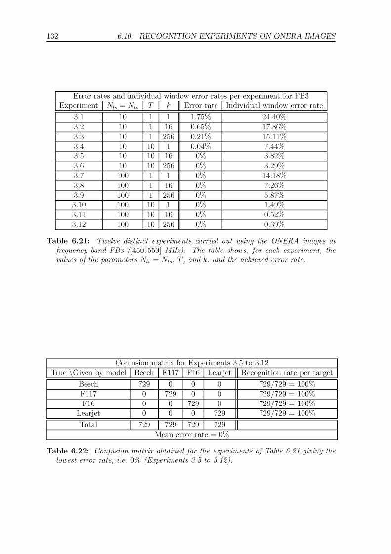
132 6.10. RECOGNITION EXPERIMENTS ON ONERA IMAGES

Error rates and individual window error rates per experiment for FB3Experiment Nls = Nts T k Error rate Individual window error rate

3.1 10 1 1 1.75% 24.40%3.2 10 1 16 0.65% 17.86%3.3 10 1 256 0.21% 15.11%3.4 10 10 1 0.04% 7.44%3.5 10 10 16 0% 3.82%3.6 10 10 256 0% 3.29%3.7 100 1 1 0% 14.18%3.8 100 1 16 0% 7.26%3.9 100 1 256 0% 5.87%3.10 100 10 1 0% 1.49%3.11 100 10 16 0% 0.52%3.12 100 10 256 0% 0.39%

Table 6.21: Twelve distinct experiments carried out using the ONERA images atfrequency band FB3 ([450; 550] MHz). The table shows, for each experiment, thevalues of the parameters Nls = Nts, T , and k, and the achieved error rate.

Confusion matrix for Experiments 3.5 to 3.12True \Given by model Beech F117 F16 Learjet Recognition rate per target

Beech 729 0 0 0 729/729 = 100%F117 0 729 0 0 729/729 = 100%F16 0 0 729 0 729/729 = 100%

Learjet 0 0 0 729 729/729 = 100%

Total 729 729 729 729Mean error rate = 0%

Table 6.22: Confusion matrix obtained for the experiments of Table 6.21 giving thelowest error rate, i.e. 0% (Experiments 3.5 to 3.12).

6.10. RECOGNITION EXPERIMENTS ON ONERA IMAGES 133

Error rates and individual window error rates per experiment for FB4Experiment Nls = Nts T k Error rate Individual window error rate

4.1 10 1 1 4.22% 32.72%4.2 10 1 16 1.13% 22.50%4.3 10 1 256 1.12% 20.51%4.4 10 10 1 0% 10.79%4.5 10 10 16 0% 6.57%4.6 10 10 256 0% 5.38%4.7 100 1 1 0% 18.43%4.8 100 1 16 0% 10.92%4.9 100 1 256 0% 8.95%4.10 100 10 1 0% 2.76%4.11 100 10 16 0% 1.16%4.12 100 10 256 0% 0.89%

Table 6.23: Twelve distinct experiments carried out using the ONERA images atfrequency band FB4 ([1.2; 1.3] GHz). The table shows, for each experiment, thevalues of the parameters Nls = Nts, T , and k, and the achieved error rate.

Confusion matrix for Experiments 4.4 to 4.12True \Given by model Beech F117 F16 Learjet Recognition rate per target

Beech 468 0 0 0 468/468 = 100%F117 0 468 0 0 468/468 = 100%F16 0 0 468 0 468/468 = 100%

Learjet 0 0 0 468 468/468 = 100%

Total 468 468 468 468Mean error rate = 0%

Table 6.24: Confusion matrix obtained for the experiments of Table 6.23 giving thelowest error rate, i.e. 0% (Experiments 4.4 to 4.12).

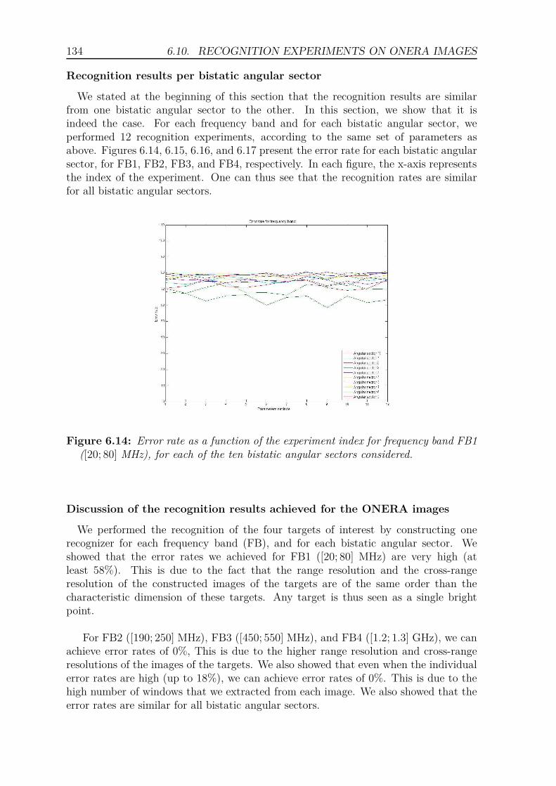
134 6.10. RECOGNITION EXPERIMENTS ON ONERA IMAGES

Recognition results per bistatic angular sector

We stated at the beginning of this section that the recognition results are similarfrom one bistatic angular sector to the other. In this section, we show that it isindeed the case. For each frequency band and for each bistatic angular sector, weperformed 12 recognition experiments, according to the same set of parameters asabove. Figures 6.14, 6.15, 6.16, and 6.17 present the error rate for each bistatic angularsector, for FB1, FB2, FB3, and FB4, respectively. In each figure, the x-axis representsthe index of the experiment. One can thus see that the recognition rates are similarfor all bistatic angular sectors.

Figure 6.14: Error rate as a function of the experiment index for frequency band FB1([20; 80] MHz), for each of the ten bistatic angular sectors considered.

Discussion of the recognition results achieved for the ONERA images

We performed the recognition of the four targets of interest by constructing onerecognizer for each frequency band (FB), and for each bistatic angular sector. Weshowed that the error rates we achieved for FB1 ([20; 80] MHz) are very high (atleast 58%). This is due to the fact that the range resolution and the cross-rangeresolution of the constructed images of the targets are of the same order than thecharacteristic dimension of these targets. Any target is thus seen as a single brightpoint.

For FB2 ([190; 250] MHz), FB3 ([450; 550] MHz), and FB4 ([1.2; 1.3] GHz), we canachieve error rates of 0%, This is due to the higher range resolution and cross-rangeresolutions of the images of the targets. We also showed that even when the individualerror rates are high (up to 18%), we can achieve error rates of 0%. This is due to thehigh number of windows that we extracted from each image. We also showed that theerror rates are similar for all bistatic angular sectors.

6.10. RECOGNITION EXPERIMENTS ON ONERA IMAGES 135

Figure 6.15: Error rate as a function of the experiment index for frequency band FB2([190; 250] MHz), for each of the ten bistatic angular sectors considered.

Figure 6.16: Error rate as a function of the experiment index for frequency band FB3([450; 550] MHz), for each of the ten bistatic angular sectors considered.

136 6.11. CONCLUSION

Figure 6.17: Error rate as a function of the experiment index for frequency band FB4([1.2; 1.3] GHz), for each of the ten bistatic angular sectors considered.

The difference between the error rates achieved for FB1 and for the three other FBsis also due to the difference in scattering mechanisms. Indeed, for FB1, the scatteringmechanisms mainly depend on the volume of the targets while, for the three other FBs,the scattering mechanisms depend on the shape of the targets. Since the four targetsof interest have different shapes but about the same volume, no clear difference couldbe made in the case of FB1.

6.11 Conclusion

In this chapter, we performed the recognition of targets by using their radar images.We first described the physical space into which airplanes fly, and the mapping fromthe physical space to the parameter space in terms of which we express the bistaticcomplex radar cross-section (BS-CRCS), the bistatic radar cross-section (BS-RCS),and the images of these airplanes. We defined the recognition strategy that we applyfor the design of the recognition stage of each of the three automatic target recognition(ATR) systems according to this parameter space. According to the recognitionstrategy we defined, we build one recognizer for each tile of the parameter space.

The recognition method is based on the joint use of window extraction andextremely randomized trees (extra-trees). We used window extraction to producefeature vectors (FVs) out of each image, for both the learning set (LS) and the testset (TS). An FV consists in a set of windows extracted out of a particular image, eachwindow being characterized by the values of the pixels inside this window. The targetclass model we built from the FVs of the LS consists of an ensemble of extra-trees.During test and operational use, the class of a target is determined by propagatingthe FV produced from the image of this target through each extra-tree of the targetclass model.

6.11. CONCLUSION 137

We motivated the use of such a recognition method by both its accuracy andefficiency that are as high as that of other classification methods. Moreover, it is, toour knowledge, one of the first use of tree-based methods in radar ATR.

We first tested our recognition method on the well-known MSTAR SAR data,which allowed us to compare the results achieved with the extra-trees-based recog-nition method to the results achieved by other recognition methods described in theliterature. Even though the ATR methods reported in the literature use differentversions of the MSTAR data, the comparison showed that the error rates we achievedusing this recognition method (error rate comprised between 1% and 3% dependingon the set of parameters) are among the best error rates reported in the literature.This proves that the extra-trees-based recognition method is an efficient method forthe recognition of radar images.

We then tested the classification method on the ONERA images. According tothe recognition strategy, we built one recognizer for each frequency band (FB) andfor each bistatic angular sector. We considered neither the azimuth angle nor theelevation angle, since it was experimentally proven that the recognition method isinsensitive to the rotation of targets. The error rates that we achieved are very highfor FB1 ([20; 80] MHz), of the order of 60%, due to the low resolution of the radarimages compared to the characteristic dimension of the targets. The error rates thatwe achieved for FB2, FB3, and FB4 are very small (about 1% to 4%), and can eventend to 0% for some particular sets of parameters. We explain theses results bythe higher resolutions of the images in these frequency bands. We also explain thedifference of the recognition results for FB1 and the three other FBs by the fact thatthe scattering mechanisms for FB1 depend more on the volumes of the target than forthe three other FBs, and by the fact that the targets of interest have about the samevolumes, but different shapes.

We will compare the recognition results we achieved in this chapter for the recog-nition of targets from their radar images to the recognition results we achieve for therecognition of these targets from their radar cross-sections, either complex or real.

138 6.11. CONCLUSION

Chapter 7

Recognition of targetsby using their bistatic RCS,either complex or real

Contents7.1 Motivation . . . . . . . . . . . . . . . . . . . . . . . . . . . . 140

7.2 Block diagram of the recognizer . . . . . . . . . . . . . . . 141

7.3 Production of feature vectors . . . . . . . . . . . . . . . . . 142

7.4 Determination of target class model by vector spaces . . . 143

7.4.1 Motivation for using subspace methods . . . . . . . . . . . . 143

7.4.2 Subspaces . . . . . . . . . . . . . . . . . . . . . . . . . . . . . 143

7.4.3 Size of subspaces . . . . . . . . . . . . . . . . . . . . . . . . . 145

7.5 Determination of the target class . . . . . . . . . . . . . . . 145

7.5.1 Orthogonal projection . . . . . . . . . . . . . . . . . . . . . . 146

7.5.2 Metrics . . . . . . . . . . . . . . . . . . . . . . . . . . . . . . 147

7.5.3 Oblique projection . . . . . . . . . . . . . . . . . . . . . . . . 148

7.6 Quantification of performance . . . . . . . . . . . . . . . . . 148

7.7 Recognition experiments . . . . . . . . . . . . . . . . . . . . 149

7.7.1 Experimental sets . . . . . . . . . . . . . . . . . . . . . . . . 149

7.7.2 Recognition results achieved for a single (Tx,Rx) pair . . . . 149

7.7.3 Recognition results achieved for three (Tx,Rx) pairs . . . . . 163

7.8 Conclusion . . . . . . . . . . . . . . . . . . . . . . . . . . . . 167

In this chapter, we perform the recognition of targets by using either their bistaticcomplex radar cross-section (BS-CRCS) or their bistatic radar cross-section (BS-RCS).Section 7.1 states the motivation for the recognition of targets by using either theirBS-CRCS or their BS-RCS. Section 7.2 describes the block diagram of the recognizer.Section 7.3 describes the production of the feature vectors. Section 7.4 describes thedetermination of the target class model. Section 7.5 describes the determination ofthe class of an unknown target based on the target class model. Section 7.6 presents

139

140 7.1. MOTIVATION

the criteria we use for the quantification of the performance of the method. Sec-tion 7.7 presents the recognition experiments we performed and the recognition rateswe achieved. Section 7.8 concludes.

7.1 Motivation for the recognition of targets by us-

ing either their bistatic complex RCS or their

bistatic RCS

In Chapter 6, we performed the recognition of targets by using their radar images.We constructed the radar images of targets from a two-dimensional (2D) array ofvalues of bistatic complex radar cross-section (BS-CRCS) of these targets. Thedimensions of this 2D array are the frequency and the bistatic angle.

However, in an operational outdoor passive-radar-based automatic target recogni-tion (ATR) system, it is unlikely that both frequency diversity and angular diversitywill be available. We explained the reasons for not being able to achieve this 2Ddiversity in Section 6.1.

To overcome the need for the necessary 2D diversity, and thus, the need formultiple transmitters (Tx’s) and multiple receivers (Rx’s), we perform, in this chapter,the recognition of targets directly according to either their BS-CRCS or their bistaticradar cross-section (BS-RCS). Therefore, we could a priori use a single (Tx,Rx) pairfor the recognition of targets.

Figure 7.1 shows the block diagram of the implemented passive-radar-based auto-matic target recognition (ATR) system. The main difference with the ATR systemdiscussed in Chapter 6 is that we do not construct images of the targets. We presentedthe extraction of both the BS-CRCS and the BS-RCS from raw data in Chapter 4. Inthis chapter, we design, implement, and test the recognition stage, i.e. the recognizer,of this ATR system.

Figure 7.1: Block diagram of our ATR system using the bistatic complex radar cross-sections or the bistatic radar cross-sections of targets.

7.2. BLOCK DIAGRAM OF THE RECOGNIZER 141

7.2 Block diagram of the recognizer

We explained our recognition strategy in Section 6.3. The input data of therecognizer are either the bistatic complex radar cross-section (BS-CRCS) or thebistatic radar cross-section (BS-RCS) of the targets of interest. The targetsof interest are a Beechcraft, an F117 fighter, an F16 fighter, and a Learjet. Eachtype of target corresponds to a particular target class. We thus consider Nc = 4 classes.

Each value of BS-CRCS or BS-RCS is associated with a value of each of theparameters of the parameter space, which are the frequency band f , the polarizationPol, the aspect angle α, and the bistatic angle β (Section 6.2). As described inSection 6.3, we divide the parameter space into tiles, and we build a recognizer foreach tile. As explained in Chapter 4, values of both the BS-CRCS and the BS-RCS areavailable for four polarizations, four frequency bands, three aspect angles, and severalbistatic angles ranging from 6◦ to 160◦. We arbitrarily divide the range of bistaticangle into 12 overlapping sectors, as described in Table 6.1, which we reproduce inTable 7.1 for convenience. We thus build 4 × 4 × 3 × 12 = 576 recognizers, one foreach polarization, for each frequency band, and for each tile of the (α, β) plane.

For each frequency band, we use the values of both the BS-CRCS and the BS-RCSthat we computed for the lower half of this frequency band for the learning set (LS),and the values of both the BS-CRCS and the BS-RCS that we computed for the upperhalf of this frequency band for the test set (TS).

Bistatic angular sector index Bistatic angular sector (degrees)

1 (6, 43.5)2 (18.5, 56)3 (31, 68.5)4 (43.5, 81)5 (56, 93.5)6 (68.5, 106)7 (81, 118.5)8 (93.5, 131)9 (106, 143.5)10 (118.5, 156)11 (131, 168.5)12 (143.5, 181)

Table 7.1: Bistatic angular sectors considered.

Figure 7.2 gives the block diagrams of the recognizer we build for any giventile. The first block diagram concerns the "construction" of the correspondingsub-recognizer, which uses the LS data for all Nc classes to produce a target classmodel consisting of a list of subspaces. We describe the determination of the targetclass model in Section 7.4. For each of the Nc classes, one first produces feature vectors(FVs). Each FV consists of an ensemble of values of either BS-CRCS or BS-RCS. We

142 7.3. PRODUCTION OF FEATURE VECTORS

describe the production of FVs in Section 7.3.

Figure 7.2: Block diagrams summarizing the architecture of any of the sub-recognizersof the recognition stage. (a) shows the successive steps in building the target classmodel, and (b) the successive steps in performing the actual recognition, either fortesting (and performance evaluation) or for operational use.

The second block diagram concerns the "test" of the (sub-)recognizer and its "oper-ational use". In both cases, one first produces one FV (at a time) from the appropriatedata for the region of interest. One then projects this FV on all Nc subspaces, andcomputes some corresponding (projection) metric. The best metric value determinesthe class that the (sub-)recognizer assigns to this FV. The difference between test (TS)and operational use (operational data) is the availability of the ground truth for theTS, which allows one to quantify the performance of the (sub-)recognizer for the regionconsidered.

7.3 Production of feature vectors

For each polarization, each frequency band, and a given region in the (α, β)plane of a specific class (i.e. with one of the indices 1 to Nc, or x), we mustproduce a set of feature vectors (FVs) from the data in this region, i.e. from (α, β)trajectories with either associated complex bistatic radar cross-section (BS-CRCS)values or associated bistatic radar cross-section (BS-RCS) values. The processfor producing the FVs is the same for any region and for any class. The follow-ing description is thus generic for the data in one region of the (α, β) plane of one class.

The size N of each FV, and the number M of FVs for this generic region mustobey the following constraints: (1) for subsequent processing, N must be the same forall classes; (2) M must be much larger than N to ensure adequate classification. The

7.4. DETERMINATION OF TARGET CLASS MODEL BY VECTOR SPACES143

value of N is chosen experimentally.

In the experiments described later, we build the FVs as follows. For each frequencyband, each polarization, and each (α, β) region, the aspect angle α has a fixed value,since the targets were kept fixed in the anechoic chamber (Chapter 4). Thus, thevariation is expressed only in terms of the bistatic angle β. Each FV represents thevariation of either the BS-CRCS or the BS-RCS during a variation of the bistatic angleof β = 25◦, for a fixed polarization pair and a fixed frequency. Several other ways ofconstructing the list and of sampling it can be envisioned, but this is not discussedhere.

7.4 Determination of the target class model by vec-

tor spaces

The target class model consists in a list of vector spaces, simply called subspaces.We first describe the motivation for using subspace methods for recognition. We thendescribe the construction of the subspaces, and the determination of the size of eachsubspace.

7.4.1 Motivation for using subspace methods for recognition

In Chapter 6, the recognizer used to classify targets by using their radar images wasbased on extremely randomized trees. Here, we propose to use another recognitionmethod based on subspace methods of pattern recognition [141]. Each class of targetis represented by the best-approximating subspace.

Subspace methods of pattern recognition were introduced by Karhunen, Kohonen,Oja, and Watanabe, and are summarized in [141]. Subspace methods of patternrecognition are used in different applications, such as speech recognition [5, 79], andimage recognition [230]. In the radar domain, subspace methods are mainly used fordetection purposes [10–12, 16, 36, 70, 96]. In particular, [15, 29, 58, 176] use subspacemethods for the detection of man-made objects in the context of foliage penetration(FOPEN) radar. To our knowledge, the use of subspace methods for radar automatictarget recognition (ATR) is novel.

Subspace methods in the context of recognition present a particular advantage.Since each target class is characterized by a particular subspace, adding a new tar-get class does not require to re-compute the entire target class model. Instead, thesubspace representing the new target class just needs to be computed, and added tothe target class model. Recognition techniques such as tree-based methods, supportvector machines (SVM), and neural networks (NN) require to recompute the targetclass model when a new class is added.

7.4.2 Subspaces

We generically denote the feature vectors (FVs) for one region and one class by xm,with m ∈ [1,M ]. A significant feature of our approach is that we represent the class

1447.4. DETERMINATION OF TARGET CLASS MODEL BY VECTOR SPACES

(for this region) by the best-approximating subspace, and that we project new FVs onit.

To give a true statistical spin to the problem, we consider that the xm’s are real-izations of a random vector x. The statistical correlation matrix of x is denoted by Rs

x

and defined as Rsx = E

{xxH

}, where E{.} is the expected-value operator. To go back

to a deterministic formulation, one can approximate Rsx as follows,

Rsx ≈ 1

M

M∑

m=1

xmxHm. (7.1)

To go further, we introduce the data matrix X obtained by juxtaposing the xm’s,i.e. X = (x1, . . . xm, . . . , xM). It is easy to see that

Rsx ≈ 1

M

M∑

m=1

xmxHm =

1

MXXH . (7.2)

We thus refer to the right-hand side as the deterministic correlation matrix, denotedby Rd

x, with

Rdx =

1

MXXH . (7.3)

We thus have Rsx ≈ Rd

x. Rdx is known to be the maximum-likelihood estimate of Rs

x.Observe that both Rs

x and Rdx have size N , typically with N ≪ M .

In the considerations to follow, it is more convenient to deal with XXH than with(1/M)XXH. We thus introduce

C = XXH , (7.4)

keeping in mind that C is not the true deterministic correlation matrix Rdx of the

xm’s, but is related to it via Rdx = (1/M)C. However, we will loosely refer to C as the

correlation matrix.

Any symmetric matrix can be diagonalized by an orthonormal matrix, i.e. by amatrix the columns of which are both orthogonal and normalized to unit length. Cbeing symmetric, we can write C = UHΛU , where U is the orthonormal matrix thecolumns of which are the eigenvectors ui of C normalized to unit length, and Λ is the di-agonal matrix the diagonal elements of which are the corresponding eigenvalues λi of C.

The eigenvalues of any real symmetric matrix are real. Furthermore, a matrix ofthe form UUH is not only symmetric but positive semi-definite, and the eigenvaluesof such a matrix are non-negative. Therefore, the eigenvalues of C are real andnon-negative.

Rather than using the correlation matrix, we could use the covariance matrix,which simply amounts to removing the mean from the random vector x or itsrealizations.

It is useful to visualize Rsx - and thus Rd

x and C - as an ellipsoid in RN if thebistatic radar cross-section (BS-RCS) is considered or in CN if the bistatic complex

7.5. DETERMINATION OF THE TARGET CLASS 145

radar cross-section (BS-CRCS) is considered, with its principal directions given by thecolumns ui of U and its "extent" along each ui by the corresponding λi. This gives aconceptual, pictorial representation of the distribution of the xm’s in relation to theui’s. The basic idea of subspace (and dimensionality-reduction) techniques is to ignorethe directions ui where the ellipsoid is relatively thin, i.e. for which the λi’s are verysmall and, especially, zero.

Let us order the λi’s by decreasing values, i.e. λ1 ≥ λ2 ≥ . . . ≥ λN , and keep onlythe ui’s corresponding to the K largest λi’s, i.e. to λ1, . . . , λK . The selected vectorsui can be used to define a subspace of RN (for BS-RCS) or of CN (for BS-CRCS).Furthermore, since the ui’s are orthonormal, they constitute a basis for this subspace,which is of size K. It is useful to introduce a matrix Q, the columns of which are the Kselected ui’s, i.e. Q = (u1, . . . , uK). Q is of size N×K and, thus, generally rectangular.It is also orthonormal, with QHQ = I, where I is the K × K identity matrix. Thismatrix Q constitutes a representation of the subspace built from the xm’s.

7.4.3 Size of subspaces

Each subspace is defined by a certain number of vectors corresponding to the Klargest singular values. The choice of the parameter K is crucial. On the one hand,if K is chosen too small, the corresponding subspace does not represent exactly thetarget class. On the other hand, if K is chosen too large, the corresponding subspacewill over-describe the target of interest.

In order to choose the best value of K, we plan to use the Time Reversal Operator(TRO), defined in [107, 117, 160–163, 233]. However, the TRO method assumes thatthe BS-CRCS and the BS-RCS of targets can be approximated by the bright pointmodel [35]. In short, the bright point model assumes that targets are made of a finitenumber of isotropic scatterers [57], which is not the case of complex targets such asairplanes. Indeed, the bright point model neglects different scattering mechanismssuch as multiple reflections.

We thus choose the size of each subspace, i.e. the number K of singular vectorsof each subspace, such that the sum of their corresponding singular values is at leastequal to some percentage γ of the sum of all singular values. We tested different valuesof γ. According to the results achieved, we choose γ equal to 95%.

7.5 Determination of the target class

In this section, we describe the determination of the class of an unknown target fromthe feature vector (FV) we produced the way described in Section 7.3. We first describethe orthogonal projection of this FV onto each of the subspaces of the target classmodel. We then describe the determination of the target class from these projections.We also describe some reasons for not using oblique projections.

146 7.5. DETERMINATION OF THE TARGET CLASS

7.5.1 Orthogonal projection

Before showing how to project on the subspace defined by an orthonormal matrixsuch as Q, let us review how to project on the subspace defined by a general rectangularmatrix A consisting of K linearly independent columns am [14]. The columns define asubspace, called the columnspace of A [193].

One can show that the matrix that projects any vector b ∈ RN (or CN) into thissubspace is given by the projection matrix [193]

P = A(AHA)−1AH . (7.5)

The result of the projection is then Pb. It is well known that any such projectionmatrix P is symmetric and such that P 2 = P (idempotency).

In the particular case where A is an orthonormal matrix, say Q, the projectionmatrix P is P = Q(QHQ)−1QH . Since QHQ = I, this reduces to

P = QQH . (7.6)

This matrix P projects any vector b into the subspace defined by the K columns ui of Q.

The result of projecting b into the subspace defined by the columns of Q is theprojection (vector)

p = Pb = QQHb . (7.7)

The component xi of this vector along ui, where i ∈ [1, K], is given by xi = uHi p. Thevector x = (x1 . . . xK)H of all the components is given by

x =

uH1...uHK

p = QHp. (7.8)

Using Eq. (7.7), one gets x = QHQQHb = (QHQ)QHb . Since QHQ = I, this reducesto

x = QHb, (7.9)

which is simply a statement of the well-known fact that the components of an arbitraryvector b ∈ RN (or in CN) corresponding to the axes of an orthonormal basis areobtained via the scalar product of b with each of the corresponding unit vectors ui.

The orthonormal matrix U containing the orthonormal eigenvectors of C clearlyplays a crucial role above. Of course, it can be obtained by performing the eigenvaluesdecomposition (EVD) of C = XXH. However, this requires the calculation of theproduct XXH . Since N is typically much smaller than M , the matrix C = XXH ,which is of size N × N , is typically of reasonable size. However, the determination ofthe value of each element of C requires the calculation of N × N scalar products ofsize 1 ×M , where M can be very large.

As it is well known, there is a way to get U quite simply by working directly withX, rather than with XXH . The solution is to use the singular value decomposition

7.5. DETERMINATION OF THE TARGET CLASS 147

(SVD) [193]. The SVD allows one to decompose any rectangular N ×M matrix X asX = UΣV H , where U is a first N ×N orthonormal matrix, Σ an N × M rectangulardiagonal matrix, and V a second M ×M orthonormal matrix.

The columns of U are called the left singular vectors of U and are denoted byui. One can show that the ui’s are the eigenvectors of C = XXH . The matrix Uobtained by SVD is thus exactly the one needed to build the matrix Q appearing inthe expression for the projection matrix P .

In summary, it is generally very advantageous to compute the required projectionmatrix Q (and the projection components xi) by using the SVD of X rather than theEVD of XXT .

7.5.2 Metrics

In our experimental work, we use four different metrics. The first metric is the normof the projection error e = b− p [141, 164,219,226], i.e.

|e| = |b− p| = |b− Pb| = |(I − P )b|, (7.10)

where P = QQH . The subspace for which the projection error is the lowest correspondsto the class labelled to vector b.

Since we are dealing with orthogonal projections, the measure of the energy of theprojection of vector b onto subspace defined by Q is equivalent to the norm of theprojection vector. It is referred to in [72,110,141,164,226] as the "basic decision rule",which is expressed as

E0 =bHPb

bHb. (7.11)

The subspace for which the energy is the largest corresponds to the class labelled tovector b. Taking the minimum of the projection error (Eq. (7.10)) is equivalent totaking the maximum of the projection ((7.11)). For coherency with the other metrics,we use Eq. (7.11) as the first metric.

The second and third metrics used also measure the energy Eρ of the projectionof vector b [141] onto subspace defined by Q. The difference with the first metric isthat the projection of vector b onto each of the vectors ui’s of Q is weighted by theratio of the singular value λi corresponding to the appropriate singular vector ui to thefirst singular value, λ1. This means that the directions of the singular vectors of eachsubspace are weighted by their corresponding singular values. The second and thirdmetrics are expressed as [113]

Eρ =K∑

i=1

(λiλ1

)ρbHuiu

Hi b

bHb, (7.12)

where ρ is a factor defining the importance of the weighting. When ρ = 0, theright-hand side of Eq. (7.12) reduces to the right-hand side of Eq. (7.11). This is whywe denoted the first metric by E0.

148 7.6. QUANTIFICATION OF PERFORMANCE

For the second metric, we choose ρ = 1, as in the Multiple Similarity Method [113].We thus denote the second metric by E1. For the third metric, we choose ρ = 0.05, asin [113]. We thus denote the third metric by E0.05. These values have proven to givethe highest classification rates, as reported in [113]. As for the first metric, the classassigned to vector b corresponds to the subspace Q for which the energy z is the highest.

The fourth metric consists in the fusion of the first three metrics. We use themajority voting rule. Each of the three metrics described above votes for a particularclass. The majority voting rule consists in assigning to an object the class for which thenumber of votes is the largest. One could also envision fusing the data according to theDempster-Schafer Theory of Evidence as in [34, 105]. This approach is not consideredhere, since the classes are mutually exclusive.

7.5.3 Oblique projection

Until now, we proposed metrics based on the orthogonal projection of a vector zonto a subspace Q. In [14], the oblique projection has been defined for detectionproblems. We thus explore the possibility of using such a metric in our work.

Let us consider that the target is modelled by a subspace H and the noise subspaceis represented by subspace S. The oblique projection onto a subspace H according todirection defined by subspace S is defined in [14] as

EHS = H(HHP⊥S H)−1HHP⊥

S , (7.13)

whereP⊥S = I − PS, (7.14)

and PS stands for the orthogonal projector onto subspace S.

While the orthogonal projection PH defined in Section 7.5.1 only requires thedefinition of the subspace H , the oblique projection requires that the subspaces H andS be both defined.

In the case of recognition, let us consider N classes, each class being representedby a subspace denoted by Hi, with i = 1 . . . N . To define the oblique projection ontosubspace H1, one could think about defining the subspace H of Eq. (7.13) as H1, andthe subspace S of Eq. (7.13) as the subspace computed from the feature vectors of allother subspaces [H2 . . .HN ]. However, this does not imply that the subspaces H andS are separated. Moreover, the addition of an extra class requires one to recomputeall the oblique projectors. Eventually, the computation of the oblique projection EHSis more computationally intensive than the computation of the orthogonal projectionPH . Therefore, the oblique projection will not be used in this work.

7.6 Quantification of performance

We quantify the performance of the recognizer during the test phase, according tothe probability of correct recognition. The probability of correct recognition is definedas the ratio of the number of feature vectors (FVs) that are correctly recognized to

7.7. RECOGNITION EXPERIMENTS 149

the total number of FVs. The probability of correct recognition is computed from theconfusion matrix, as described in Section 6.8.

7.7 Recognition experiments

We first describe the experimental sets we use for the recognition experiments. Wethen present the recognition results achieved for a single transmitter (Tx) and a singlereceiver (Rx), and for three (Tx,Rx) pairs. For each case, the recognition results arepresented for the use of both the bistatic complex radar cross-sections (BS-CRCSs) andthe bistatic radar cross-sections (BS-RCSs) of targets. We then discuss the differentresults achieved.

7.7.1 Experimental sets

BS-CRCSs and BS-RCSs of targets are available for four frequency bands and forfour polarizations. For each frequency band and for each polarization, we divide theparameter space (α, β) into 3 × 12 overlapping tiles, where 3 is the number of aspectangles of the targets, and 12 the number of bistatic angular sectors considered. Asdescribed in Section 7.2, we build one recognizer for each tile. Therefore, we build atotal of 4 × 4 × 3 × 12 = 576 recognizers.

We first consider only a single (Tx,Rx) pair. We thus perform 576 recognitionexperiments, one per recognizer. We give the recognition results in Section 7.7.2 foreach frequency band and for each polarization.

We then consider multiple (Tx,Rx) pairs. For computational reasons, we chooseto consider three (Tx,Rx) pairs, with a single Tx operating on a particular frequencyand a particular polarization, and three Rx’s. All three Rx’s operate on the samepolarization, either H or V , which can be distinct from the polarization of the Tx.The three Rx’s are assumed to operate at locations that differ in bistatic angle. Thereare thus C3

12 = 220 possible combinations of the three receivers, for each polarization,and each frequency band. We thus perform 4 × 4 × 3 × 220 = 10560 experiments. Asfor the case of a single (Tx,Rx) pair, we give the recognition results for each frequencyband and for each polarization.

Table 7.2 lists the different recognition experiments we performed. Each experimentis assigned a label n1.n2, where n1 stands for the number of (Tx,Rx) pairs we consider,and n2 stands for the frequency band, and whose third digit stands for the polarizationused.

7.7.2 Recognition results achieved for a single (Tx,Rx) pair

We present the results achieved for a single (Tx,Rx) pair, and by using either theBS-CRCS or the BS-RCS of the targets to classify. For both the BS-CRCS and theBS-RCS cases, we show the recognition rate for each of the four metrics that we in-troduced in Section 7.5.2. For conciseness, we present in details the results achievedfor the HH polarization pair. The results achieved for the three other polarizationpairs are similar to the results achieved for the HH polarization pair. Thus, referring

150 7.7. RECOGNITION EXPERIMENTS

Experimentindex for1 (Tx,Rx)pair

Experimentindex for3 (Tx,Rx)pairs

Frequencyband

Polarization Aspectangles

Bistaticangularsectors

Numberof experi-ments

Exp. 1.1.1 Exp. 2.1.1 [20; 80]MHz

HH All (3) All (12) 36

Exp. 1.1.2 Exp. 2.1.2 [20; 80]MHz

HV All (3) All (12) 36

Exp. 1.1.3 Exp. 2.1.3 [20; 80]MHz

V H All (3) All (12) 36

Exp. 1.1.4 Exp. 2.1.4 [20; 80]MHz

V V All (3) All (12) 36

Exp. 1.2.1 Exp. 2.2.1 [190; 250]MHz

HH All (3) All (12) 36

Exp. 1.2.2 Exp. 2.2.2 [190; 250]MHz

HV All (3) All (12) 36

Exp. 1.2.3 Exp. 2.2.3 [190; 250]MHz

V H All (3) All (12) 36

Exp. 1.2.4 Exp. 2.2.4 [190; 250]MHz

V V All (3) All (12) 36

Exp. 1.3.1 Exp. 2.3.1 [450; 550]MHz

HH All (3) All (12) 36

Exp. 1.3.2 Exp. 2.3.2 [450; 550]MHz

HV All (3) All (12) 36

Exp. 1.3.3 Exp. 2.3.3 [450; 550]MHz

V H All (3) All (12) 36

Exp. 1.3.4 Exp. 2.3.4 [450; 550]MHz

V V All (3) All (12) 36

Exp. 1.4.1 Exp. 2.4.1 [1.2; 1.3]GHz

HH All (3) All (12) 36

Exp. 1.4.2 Exp. 2.4.2 [1.2; 1.3]GHz

HV All (3) All (12) 36

Exp. 1.4.3 Exp. 2.4.3 [1.2; 1.3]GHz

V H All (3) All (12) 36

Exp. 1.4.4 Exp. 2.4.4 [1.2; 1.3]GHz

V V All (3) All (12) 36

Total number of experiments 576

Table 7.2: Recognition experiments performed.

7.7. RECOGNITION EXPERIMENTS 151

to Table 7.2, we present the results for the recognition Experiments 1.1.1, 1.2.1, 1.3.1,and 1.4.1, i.e. experiments for each frequency band and for the HH polarization.

Probabilities of correct recognition for FB1 ([20; 80] MHz)

Tables 7.3, 7.4, 7.5, and 7.6 present the probabilities of correct recognition obtainedfor the recognition of targets for the first frequency band, FB1 ([20; 80] MHz), for thecriteria E0, E1, E0.05, and for the aggregation of these three criteria, respectively. Asone can see on the four tables, the probability of correct recognition is always very lowfor either the BS-CRCS or the BS-RCS, ranging from 0.25, which is the probability ofcorrect recognition that would be obtained by recognizing targets randomly, and 0.63,depending on the tile of the (α, β) plane, and on the metric used. The reasons forsuch a low probability of correct recognition are that the BS-CRCS and the BS-RCSvary more with volume than with shape at these frequencies, and that the targets haveabout the same volume, as discussed in Chapter 4.

Probabilities of correct recognition for FB1For BS-CRCS For BS-RCS

α = 0◦ α = 45◦ α = 90◦ α = 0◦ α = 45◦ α = 90◦

β ∈ [6◦, 43.5◦] 0.41 0.33 0.45 0.36 0.32 0.38β ∈ [18.5◦, 56◦] 0.57 0.55 0.60 0.34 0.35 0.47β ∈ [31◦, 68.5◦] 0.57 0.48 0.53 0.33 0.34 0.30β ∈ [43.5◦, 81◦] 0.60 0.45 0.38 0.31 0.29 0.35β ∈ [56◦, 93.5◦] 0.50 0.27 0.47 0.34 0.35 0.30β ∈ [68.5◦, 106◦] 0.32 0.25 0.48 0.35 0.31 0.34β ∈ [81◦, 118.5◦] 0.35 0.32 0.31 0.32 0.29 0.33β ∈ [93.5◦, 131◦] 0.39 0.32 0.36 0.27 0.34 0.34β ∈ [106◦, 143.5◦] 0.63 0.32 0.33 0.37 0.38 0.35β ∈ [118.5◦, 156◦] 0.42 0.33 0.47 0.33 0.34 0.34

Table 7.3: Probabilities of correct recognition, shown tile-by-tile, for metric E0

applied to BS-CRCS and BS-RCS, computed for the frequency band FB1 ([20; 80]MHz) and polarization HH. The table is divided in tiles in the same way as the(α, β) plane is.

152 7.7. RECOGNITION EXPERIMENTS

Probabilities of correct recognition for FB1For BS-CRCS For BS-RCS

α = 0◦ α = 45◦ α = 90◦ α = 0◦ α = 45◦ α = 90◦

β ∈ [6◦, 43.5◦] 0.46 0.46 0.41 0.36 0.33 0.38β ∈ [18.5◦, 56◦] 0.60 0.50 0.44 0.42 0.47 0.44β ∈ [31◦, 68.5◦] 0.63 0.44 0.47 0.31 0.41 0.51β ∈ [43.5◦, 81◦] 0.55 0.37 0.41 0.35 0.33 0.39β ∈ [56◦, 93.5◦] 0.49 0.39 0.39 0.34 0.35 0.36β ∈ [68.5◦, 106◦] 0.50 0.52 0.43 0.33 0.38 0.34β ∈ [81◦, 118.5◦] 0.63 0.47 0.37 0.39 0.37 0.34β ∈ [93.5◦, 131◦] 0.54 0.48 0.40 0.39 0.35 0.36β ∈ [106◦, 143.5◦] 0.38 0.49 0.34 0.39 0.42 0.31β ∈ [118.5◦, 156◦] 0.42 0.5 0.29 0.40 0.40 0.31

Table 7.4: Probabilities of correct recognition, shown tile-by-tile, for metric E1

applied to BS-CRCS and BS-RCS, computed for the frequency band FB1 ([20; 80]MHz) and polarization HH. The table is divided in tiles in the same way as the(α, β) plane is.

Probabilities of correct recognition for FB1For BS-CRCS For BS-RCS

α = 0◦ α = 45◦ α = 90◦ α = 0◦ α = 45◦ α = 90◦

β ∈ [6◦, 43.5◦] 0.42 0.38 0.36 0.36 0.32 0.40β ∈ [18.5◦, 56◦] 0.52 0.42 0.39 0.36 0.43 0.49β ∈ [31◦, 68.5◦] 0.49 0.42 0.34 0.33 0.39 0.48β ∈ [43.5◦, 81◦] 0.48 0.35 0.31 0.35 0.35 0.39β ∈ [56◦, 93.5◦] 0.45 0.37 0.36 0.37 0.38 0.32β ∈ [68.5◦, 106◦] 0.41 0.41 0.38 0.37 0.40 0.38β ∈ [81◦, 118.5◦] 0.51 0.35 0.32 0.36 0.39 0.36β ∈ [93.5◦, 131◦] 0.42 0.41 0.29 0.32 0.38 0.36β ∈ [106◦, 143.5◦] 0.29 0.40 0.26 0.36 0.43 0.35β ∈ [118.5◦, 156◦] 0.32 0.43 0.24 0.37 0.38 0.33

Table 7.5: Probabilities of correct recognition, shown tile-by-tile, for metric E0.05

applied to BS-CRCS and BS-RCS, computed for the frequency band FB1 ([20; 80]MHz) and polarization HH. The table is divided in tiles in the same way as the(α, β) plane is.

7.7. RECOGNITION EXPERIMENTS 153

Probabilities of correct recognition for FB1For BS-CRCS For BS-RCS

α = 0◦ α = 45◦ α = 90◦ α = 0◦ α = 45◦ α = 90◦

β ∈ [6◦, 43.5◦] 0.47 0.47 0.41 0.37 0.33 0.41β ∈ [18.5◦, 56◦] 0.63 0.51 0.45 0.42 0.46 0.47β ∈ [31◦, 68.5◦] 0.63 0.47 0.46 0.33 0.40 0.51β ∈ [43.5◦, 81◦] 0.55 0.39 0.41 0.36 0.34 0.41β ∈ [56◦, 93.5◦] 0.52 0.41 0.38 0.34 0.39 0.33β ∈ [68.5◦, 106◦] 0.49 0.50 0.42 0.36 0.41 0.37β ∈ [81◦, 118.5◦] 0.63 0.48 0.38 0.41 0.38 0.36β ∈ [93.5◦, 131◦] 0.49 0.49 0.37 0.43 0.39 0.38β ∈ [106◦, 143.5◦] 0.35 0.48 0.32 0.37 0.43 0.32β ∈ [118.5◦, 156◦] 0.42 0.51 0.30 0.36 0.40 0.35

Table 7.6: Probabilities of correct recognition, shown tile-by-tile, for the aggrega-

tion of the three metrics applied to BS-RCS and BS-RCS, computed for thefrequency band FB1 ([20; 80] MHz) and polarization HH. The table is divided intiles in the same way as the (α, β) plane is.

154 7.7. RECOGNITION EXPERIMENTS

Probabilities of correct recognition for FB2 ([190; 250] MHz)

Tables 7.7, 7.8, 7.9, and 7.10 present the probabilities of correct recognition obtainedfor the recognition of targets for the second frequency band, FB2 ([190; 250] MHz), forthe criteria E0, E1, E0.05, and for the aggregation of these three criteria, respectively.The probability of correct recognition ranges from 0.32 to 0.90, depending on the tileof the (α, β) plane, and on the metric used. The probabilities of correct recognitionare higher than for the lowest frequency band when using either the BS-CRCSs or theBS-RCSs. This can be explained by the fact that the BS-CRCS is influenced by boththe volume of the targets, as at the lowest frequency band, and the shape of the targets.One can also see that, for a constant β, the highest probabilities of correct recognitionare obtained for α = 0◦. This is due to the shape of the targets. No bistatic angularsector seems to be preferable. When using BS-CRCSs, metric E0, that does not weightthe vectors of the subspaces, appears to give better results than the weighting metricsE1 and E0.05, while, when using BS-RCSs, metric E0.05 appears to give the best results.

Probabilities of correct recognition for FB2For BS-CRCS For BS-RCS

α = 0◦ α = 45◦ α = 90◦ α = 0◦ α = 45◦ α = 90◦

β ∈ [6◦, 43.5◦] 0.80 0.78 0.68 0.43 0.49 0.40β ∈ [18.5◦, 56◦] 0.84 0.65 0.81 0.53 0.41 0.64β ∈ [31◦, 68.5◦] 0.68 0.69 0.72 0.48 0.40 0.67β ∈ [43.5◦, 81◦] 0.73 0.47 0.78 0.43 0.38 0.43β ∈ [56◦, 93.5◦] 0.64 0.62 0.50 0.57 0.55 0.40β ∈ [68.5◦, 106◦] 0.74 0.56 0.58 0.59 0.48 0.41β ∈ [81◦, 118.5◦] 0.72 0.66 0.66 0.57 0.38 0.39β ∈ [93.5◦, 131◦] 0.90 0.57 0.55 0.67 0.43 0.44β ∈ [106◦, 143.5◦] 0.86 0.68 0.59 0.52 0.49 0.45β ∈ [118.5◦, 156◦] 0.87 0.67 0.64 0.50 0.58 0.48

Table 7.7: Probabilities of correct recognition, shown tile-by-tile, for metric E0

applied to BS-CRCS and BS-RCS, computed for the frequency band FB2 ([190; 250]MHz) and polarization HH. The table is divided in tiles in the same way as the(α, β) plane is.

7.7. RECOGNITION EXPERIMENTS 155

Probabilities of correct recognition for FB2For BS-CRCS For BS-RCS

α = 0◦ α = 45◦ α = 90◦ α = 0◦ α = 45◦ α = 90◦

β ∈ [6◦, 43.5◦] 0.73 0.56 0.50 0.45 0.42 0.36β ∈ [18.5◦, 56◦] 0.80 0.58 0.76 0.53 0.37 0.57β ∈ [31◦, 68.5◦] 0.74 0.52 0.78 0.49 0.32 0.63β ∈ [43.5◦, 81◦] 0.71 0.50 0.63 0.45 0.42 0.47β ∈ [56◦, 93.5◦] 0.77 0.66 0.60 0.48 0.47 0.53β ∈ [68.5◦, 106◦] 0.76 0.62 0.48 0.52 0.41 0.39β ∈ [81◦, 118.5◦] 0.67 0.56 0.52 0.44 0.35 0.42β ∈ [93.5◦, 131◦] 0.81 0.65 0.64 0.50 0.34 0.42β ∈ [106◦, 143.5◦] 0.81 0.70 0.59 0.53 0.39 0.50β ∈ [118.5◦, 156◦] 0.82 0.71 0.58 0.60 0.51 0.45

Table 7.8: Probabilities of correct recognition, shown tile-by-tile, for metric E1

applied to BS-CRCS and BS-RCS, computed for the frequency band FB2 ([190; 250]MHz) and polarization HH. The table is divided in tiles in the same way as the(α, β) plane is.

Probabilities of correct recognition for FB2For BS-CRCS For BS-RCS

α = 0◦ α = 45◦ α = 90◦ α = 0◦ α = 45◦ α = 90◦

β ∈ [6◦, 43.5◦] 0.60 0.43 0.35 0.52 0.53 0.41β ∈ [18.5◦, 56◦] 0.61 0.45 0.62 0.60 0.47 0.69β ∈ [31◦, 68.5◦] 0.62 0.39 0.60 0.54 0.41 0.69β ∈ [43.5◦, 81◦] 0.52 0.40 0.48 0.48 0.45 0.51β ∈ [56◦, 93.5◦] 0.52 0.57 0.47 0.59 0.63 0.55β ∈ [68.5◦, 106◦] 0.59 0.49 0.41 0.65 0.54 0.44β ∈ [81◦, 118.5◦] 0.60 0.47 0.41 0.59 0.41 0.43β ∈ [93.5◦, 131◦] 0.67 0.47 0.54 0.69 0.47 0.46β ∈ [106◦, 143.5◦] 0.57 0.54 0.49 0.56 0.51 0.49β ∈ [118.5◦, 156◦] 0.67 0.53 0.41 0.68 0.66 0.51

Table 7.9: Probabilities of correct recognition, shown tile-by-tile, for metric E0.05

applied to BS-CRCS and BS-RCS, computed for the frequency band FB2 ([190; 250]MHz) and polarization HH. The table is divided in tiles in the same way as the(α, β) plane is.

156 7.7. RECOGNITION EXPERIMENTS

Probabilities of correct recognition for FB2For BS-CRCS For BS-RCS

α = 0◦ α = 45◦ α = 90◦ α = 0◦ α = 45◦ α = 90◦

β ∈ [6◦, 43.5◦] 0.74 0.59 0.47 0.56 0.54 0.41β ∈ [18.5◦, 56◦] 0.8 0.55 0.75 0.64 0.46 0.66β ∈ [31◦, 68.5◦] 0.74 0.49 0.78 0.56 0.40 0.70β ∈ [43.5◦, 81◦] 0.67 0.49 0.62 0.50 0.47 0.57β ∈ [56◦, 93.5◦] 0.73 0.68 0.58 0.58 0.59 0.62β ∈ [68.5◦, 106◦] 0.75 0.60 0.48 0.69 0.53 0.45β ∈ [81◦, 118.5◦] 0.71 0.55 0.53 0.58 0.44 0.47β ∈ [93.5◦, 131◦] 0.82 0.62 0.65 0.72 0.49 0.48β ∈ [106◦, 143.5◦] 0.79 0.70 0.60 0.61 0.53 0.55β ∈ [118.5◦, 156◦] 0.82 0.68 0.57 0.71 0.64 0.52

Table 7.10: Probabilities of correct recognition, shown tile-by-tile, for the aggrega-

tion of the three metrics applied to BS-CRCS and BS-RCS, computed for thefrequency band FB2 ([190; 250] MHz) and polarization HH. The table is divided intiles in the same way as the (α, β) plane is.

7.7. RECOGNITION EXPERIMENTS 157

Probabilities of correct recognition for FB3 ([450; 550] MHz)

Tables 7.11, 7.12, 7.13, and 7.14 present the probabilities of correct recognitionobtained for the recognition of targets for the third frequency band, FB3 ([450; 550]MHz), for the criteria E0, E1, E0.05, and for the aggregation of these three criteria,respectively. The probability of correct recognition ranges between 0.36 and 0.98,depending on the tile of the (α, β) plane, and on the metric used. The probability ofcorrect recognition is better than for FB1 and FB2. This is explained by the fact that,for FB3, the shape of the targets influence the BS-CRCS more than their volume, asdepicted in Chapter 6. The same other conclusions can be drawn as for FB2.

Probabilities of correct recognition for FB3For BS-CRCS For BS-RCS

α = 0◦ α = 45◦ α = 90◦ α = 0◦ α = 45◦ α = 90◦

β ∈ [6◦, 43.5◦] 0.85 0.88 0.77 0.65 0.72 0.54β ∈ [18.5◦, 56◦] 0.89 0.58 0.89 0.66 0.54 0.68β ∈ [31◦, 68.5◦] 0.79 0.56 0.95 0.58 0.52 0.68β ∈ [43.5◦, 81◦] 0.93 0.72 0.93 0.61 0.36 0.67β ∈ [56◦, 93.5◦] 0.96 0.88 0.65 0.81 0.46 0.58β ∈ [68.5◦, 106◦] 0.98 0.78 0.84 0.87 0.64 0.52β ∈ [81◦, 118.5◦] 0.96 0.75 0.92 0.79 0.63 0.56β ∈ [93.5◦, 131◦] 0.97 0.64 0.81 0.72 0.63 0.56β ∈ [106◦, 143.5◦] 0.96 0.90 0.79 0.72 0.74 0.59β ∈ [118.5◦, 156◦] 0.93 0.88 0.82 0.72 0.78 0.57

Table 7.11: Probabilities of correct recognition, shown tile-by-tile, for metric E0

applied to BS-CRCS and BS-RCS, computed for the frequency band FB3 ([450; 550]MHz) and polarization HH. The table is divided in tiles in the same way as the(α, β) plane is.

158 7.7. RECOGNITION EXPERIMENTS

Probabilities of correct recognition for FB3For BS-CRCS For BS-RCS

α = 0◦ α = 45◦ α = 90◦ α = 0◦ α = 45◦ α = 90◦

β ∈ [6◦, 43.5◦] 0.77 0.63 0.59 0.56 0.46 0.42β ∈ [18.5◦, 56◦] 0.86 0.73 0.85 0.63 0.45 0.53β ∈ [31◦, 68.5◦] 0.73 0.71 0.81 0.52 0.41 0.57β ∈ [43.5◦, 81◦] 0.85 0.60 0.78 0.55 0.46 0.53β ∈ [56◦, 93.5◦] 0.73 0.78 0.76 0.48 0.47 0.58β ∈ [68.5◦, 106◦] 0.92 0.80 0.58 0.70 0.57 0.38β ∈ [81◦, 118.5◦] 0.82 0.77 0.60 0.61 0.52 0.51β ∈ [93.5◦, 131◦] 0.78 0.82 0.76 0.52 0.60 0.56β ∈ [106◦, 143.5◦] 0.83 0.83 0.70 0.48 0.56 0.58β ∈ [118.5◦, 156◦] 0.92 0.73 0.59 0.65 0.54 0.37

Table 7.12: Probabilities of correct recognition, shown tile-by-tile, for metric E1

applied to BS-CRCS and BS-RCS, computed for the frequency band FB3 ([450; 550]MHz) and polarization HH. The table is divided in tiles in the same way as the(α, β) plane is.

Probabilities of correct recognition for FB3For BS-CRCS For BS-RCS

α = 0◦ α = 45◦ α = 90◦ α = 0◦ α = 45◦ α = 90◦

β ∈ [6◦, 43.5◦] 0.62 0.53 0.40 0.76 0.73 0.56β ∈ [18.5◦, 56◦] 0.66 0.54 0.69 0.77 0.62 0.77β ∈ [31◦, 68.5◦] 0.62 0.55 0.64 0.68 0.56 0.72β ∈ [43.5◦, 81◦] 0.68 0.48 0.61 0.72 0.44 0.71β ∈ [56◦, 93.5◦] 0.54 0.65 0.58 0.83 0.60 0.70β ∈ [68.5◦, 106◦] 0.72 0.66 0.46 0.92 0.74 0.56β ∈ [81◦, 118.5◦] 0.65 0.62 0.52 0.87 0.67 0.65β ∈ [93.5◦, 131◦] 0.62 0.58 0.67 0.81 0.70 0.68β ∈ [106◦, 143.5◦] 0.70 0.65 0.51 0.75 0.79 0.71β ∈ [118.5◦, 156◦] 0.64 0.66 0.45 0.74 0.82 0.60

Table 7.13: Probabilities of correct recognition, shown tile-by-tile, for metric E0.05

applied to BS-CRCS and BS-RCS, computed for the frequency band FB3 ([450; 550]MHz) and polarization HH. The table is divided in tiles in the same way as the(α, β) plane is.

7.7. RECOGNITION EXPERIMENTS 159

Probabilities of correct recognition for FB3For BS-CRCS For BS-RCS

α = 0◦ α = 45◦ α = 90◦ α = 0◦ α = 45◦ α = 90◦

β ∈ [6◦, 43.5◦] 0.77 0.66 0.54 0.75 0.70 0.60β ∈ [18.5◦, 56◦] 0.84 0.71 0.85 0.77 0.63 0.76β ∈ [31◦, 68.5◦] 0.76 0.70 0.80 0.67 0.57 0.72β ∈ [43.5◦, 81◦] 0.85 0.60 0.76 0.73 0.47 0.69β ∈ [56◦, 93.5◦] 0.73 0.81 0.75 0.82 0.61 0.71β ∈ [68.5◦, 106◦] 0.91 0.81 0.57 0.92 0.72 0.55β ∈ [81◦, 118.5◦] 0.83 0.78 0.62 0.86 0.64 0.65β ∈ [93.5◦, 131◦] 0.77 0.79 0.80 0.83 0.74 0.70β ∈ [106◦, 143.5◦] 0.83 0.83 0.70 0.77 0.80 0.77β ∈ [118.5◦, 156◦] 0.90 0.76 0.58 0.77 0.77 0.57

Table 7.14: Probabilities of correct recognition, shown tile-by-tile, for the aggrega-

tion of the three metrics applied to BS-CRCS and BS-RCS, computed for thefrequency band FB3 ([450; 550] MHz) and polarization HH. The table is divided intiles in the same way as the (α, β) plane is.

160 7.7. RECOGNITION EXPERIMENTS

Probabilities of correct recognition for FB4 ([1.2; 1.3] GHz)

Tables 7.15, 7.16, 7.17, and 7.18 present the probabilities of correct recognitionobtained for the recognition of targets for the fourth frequency band, FB4 ([1.2; 1.3]GHz), for the criteria E0, E1, E0.05, and for the aggregation of these three criteria,respectively. The probability of correct recognition ranges from 0.27 to 1, dependingon the tile of the (α, β) plane, and on the metric used. The same conclusions can bedrawn as for FB3.

Probabilities of correct recognition for FB4For BS-CRCS For BS-RCS

α = 0◦ α = 45◦ α = 90◦ α = 0◦ α = 45◦ α = 90◦

β ∈ [6◦, 43.5◦] 1.0 0.77 0.67 0.73 0.27 0.48β ∈ [18.5◦, 56◦] 0.99 0.95 0.98 0.56 0.60 0.84β ∈ [31◦, 68.5◦] 0.99 0.84 0.96 0.68 0.53 0.83β ∈ [43.5◦, 81◦] 0.99 0.79 0.93 0.68 0.36 0.78β ∈ [56◦, 93.5◦] 1.0 0.91 0.92 0.83 0.33 0.81β ∈ [68.5◦, 106◦] 1.0 0.93 0.94 0.83 0.63 0.59β ∈ [81◦, 118.5◦] 1.0 0.86 0.98 0.84 0.66 0.59β ∈ [93.5◦, 131◦] 0.99 0.94 0.86 0.73 0.73 0.61β ∈ [106◦, 143.5◦] 1.0 0.91 0.95 0.75 0.84 0.65β ∈ [118.5◦, 156◦] 0.96 0.97 0.92 0.62 0.81 0.63

Table 7.15: Probabilities of correct recognition, shown tile-by-tile, for metric E0

applied to BS-CRCS and BS-RCS, computed for the frequency band FB4 ([1.2; 1.3]GHz) and polarization HH. The table is divided in tiles in the same way as the(α, β) plane is.

7.7. RECOGNITION EXPERIMENTS 161

Probabilities of correct recognition for FB4For BS-CRCS For BS-RCS

α = 0◦ α = 45◦ α = 90◦ α = 0◦ α = 45◦ α = 90◦

β ∈ [6◦, 43.5◦] 0.76 0.69 0.75 0.64 0.37 0.44β ∈ [18.5◦, 56◦] 0.89 0.88 0.89 0.52 0.49 0.50β ∈ [31◦, 68.5◦] 0.90 0.78 0.90 0.52 0.48 0.67β ∈ [43.5◦, 81◦] 0.89 0.81 0.80 0.53 0.46 0.65β ∈ [56◦, 93.5◦] 0.84 0.81 0.82 0.58 0.58 0.64β ∈ [68.5◦, 106◦] 0.87 0.84 0.67 0.70 0.51 0.39β ∈ [81◦, 118.5◦] 0.83 0.83 0.67 0.66 0.41 0.61β ∈ [93.5◦, 131◦] 0.88 0.77 0.71 0.61 0.55 0.60β ∈ [106◦, 143.5◦] 0.91 0.85 0.78 0.58 0.61 0.53β ∈ [118.5◦, 156◦] 0.80 0.82 0.70 0.59 0.46 0.41

Table 7.16: Probabilities of correct recognition, shown tile-by-tile, for metric E1

applied to BS-CRCS and BS-RCS, computed for the frequency band FB4 ([1.2; 1.3]GHz) and polarization HH. The table is divided in tiles in the same way as the(α, β) plane is.

Probabilities of correct recognition for FB4For BS-CRCS For BS-RCS

α = 0◦ α = 45◦ α = 90◦ α = 0◦ α = 45◦ α = 90◦

β ∈ [6◦, 43.5◦] 0.68 0.58 0.59 0.85 0.33 0.51β ∈ [18.5◦, 56◦] 0.82 0.68 0.78 0.68 0.67 0.86β ∈ [31◦, 68.5◦] 0.75 0.65 0.81 0.78 0.61 0.85β ∈ [43.5◦, 81◦] 0.75 0.65 0.75 0.72 0.48 0.83β ∈ [56◦, 93.5◦] 0.64 0.69 0.69 0.87 0.50 0.84β ∈ [68.5◦, 106◦] 0.74 0.71 0.49 0.94 0.74 0.63β ∈ [81◦, 118.5◦] 0.70 0.67 0.53 0.92 0.71 0.74β ∈ [93.5◦, 131◦] 0.71 0.62 0.50 0.80 0.84 0.81β ∈ [106◦, 143.5◦] 0.74 0.73 0.56 0.78 0.90 0.77β ∈ [118.5◦, 156◦] 0.70 0.75 0.53 0.75 0.85 0.75

Table 7.17: Probabilities of correct recognition, shown tile-by-tile, for metric E0.05

applied to BS-CRCS and BS-RCS, computed for the frequency band FB4 ([1.2; 1.3]GHz) and polarization HH. The table is divided in tiles in the same way as the(α, β) plane is.

162 7.7. RECOGNITION EXPERIMENTS

Probabilities of correct recognition for FB4For BS-CRCS For BS-RCS

α = 0◦ α = 45◦ α = 90◦ α = 0◦ α = 45◦ α = 90◦

β ∈ [6◦, 43.5◦] 0.78 0.70 0.75 0.85 0.34 0.50β ∈ [18.5◦, 56◦] 0.91 0.87 0.90 0.67 0.65 0.81β ∈ [31◦, 68.5◦] 0.90 0.78 0.91 0.75 0.58 0.85β ∈ [43.5◦, 81◦] 0.90 0.81 0.82 0.74 0.57 0.83β ∈ [56◦, 93.5◦] 0.86 0.83 0.83 0.85 0.58 0.84β ∈ [68.5◦, 106◦] 0.91 0.86 0.66 0.92 0.73 0.63β ∈ [81◦, 118.5◦] 0.89 0.84 0.68 0.88 0.70 0.75β ∈ [93.5◦, 131◦] 0.89 0.78 0.68 0.79 0.83 0.79β ∈ [106◦, 143.5◦] 0.92 0.87 0.76 0.78 0.85 0.76β ∈ [118.5◦, 156◦] 0.83 0.86 0.69 0.78 0.75 0.76

Table 7.18: Probabilities of correct recognition, shown tile-by-tile, for the aggrega-

tion of the three metrics applied to BS-CRCS and BS-RCS, computed for thefrequency band FB4 ([1.2; 1.3] GHz) and polarization HH. The table is divided intiles in the same way as the (α, β) plane is.

7.7. RECOGNITION EXPERIMENTS 163

Discussion of the recognition results achieved for a single (Tx,Rx) pair

We showed above that, for a particular frequency band and for a particularpolarization, the probability of correct recognition varies according to the tile of the(α, β) plane, and according to the metric used. While it appears that there is noparticular bistatic angular sector that favors a high probability of correct recognition,the value α = 0◦ gives a higher probability of correct recognition, for any value of β,when considering the BS-CRCS. This can be explained by the fact that the shapes ofthe front of the targets are very different, while the shapes of the sides of the targetsare rather similar. When considering the BS-RCS of targets, no particular value of αseems to be preferable.

The best metric appears to be the non-weighting metric E0 when using BS-CRCS.This means that the vectors of the subspaces must be considered of equal importance.When using BS-RCS, the best metric appears to be metric E0.05, thus giving moreimportance to the vectors corresponding to the largest eigenvalues.

To illustrate the variation of the probability of correct recognition with frequencyand polarization, the overall probability of correct recognition achieved for eachfrequency band, each polarization, and each metric, when considering the BS-CRCSof targets, is shown in Table 7.19, and in Table 7.20 when considering the BS-RCS oftargets. One can clearly see that the probability of correct recognition increases withfrequency. This is explained by the fact that, for the higher frequencies considered, theBS-CRCS is more influenced by the shape of the targets than by their volume, whileit is exactly the opposite at the lower frequencies considered. One can also see thatwe achieve the highest probabilities of correct recognition for the HH polarization,even though the probabilities of correct recognition we achieve for the three otherpolarizations are not much smaller. This can be intuitively understood by the factthat the shapes of the different targets differ more according to their horizontalplanes than their vertical planes. One can also see that the E0 metric gives the bestprobabilities of correct recognition when considering BS-CRCS, and that the metricE0.05 gives the best probabilities of correct recognition when considering BS-RCS.

We achieve higher probabilities of correct recognition for the BS-CRCS of targetsthan for their BS-RCS. For FB2, FB3, and FB4, the difference is on the order of 10%to 20%, when comparing the results of the best metric for each case. The phase ofthe BS-CRCS differs from one airplane to the other, and is thus significant for therecognition of these four targets.

7.7.3 Recognition results achieved for three (Tx,Rx) pairs

We showed in Section 7.7.2 the probabilities of correct recognition we achievedwhen considering either the BS-CRCS or the BS-RCS of the targets of interest, and asingle (Tx,Rx) pair. This means that we considered a one-dimensional (1D) diversity(the bistatic angle). In Chapter 6, we achieved probabilities of correct recognition ofabout 1 for the frequency bands FB2, FB3, and FB4. As we explained in Chapter 5,we built the radar images from the BS-CRCS extracted with a 2D diversity. In orderto increase the diversity of the data used to recognize targets, and thus in order tohopefully increase the probability of correct recognition, we can use multiple (Tx,Rx)

164 7.7. RECOGNITION EXPERIMENTS

Overall probabilities of correct recognition for BS-CRCSFrequencyband

Polarization Metric E0 Metric E1 Metric E0.05 Aggregation

FB1: [20; 80]MHz

HH 0.43 0.46 0.38 0.46

FB1: [20; 80]MHz

HV 0.37 0.42 0.39 0.43

FB1: [20; 80]MHz

V H 0.34 0.38 0.34 0.38

FB1: [20; 80]MHz

V V 0.38 0.47 0.44 0.48

FB2:[190; 250]MHz

HH 0.69 0.66 0.52 0.65

FB2:[190; 250]MHz

HV 0.60 0.60 0.49 0.60

FB2:[190; 250]MHz

V H 0.62 0.61 0.48 0.60

FB2:[190; 250]MHz

V V 0.63 0.59 0.50 0.60

FB3:[450; 550]MHz

HH 0.84 0.76 0.60 0.75

FB3:[450; 550]MHz

HV 0.76 0.69 0.54 0.69

FB3:[450; 550]MHz

V H 0.82 0.69 0.54 0.69

FB3:[450; 550]MHz

V V 0.79 0.70 0.56 0.70

FB4: [1.2; 1.3]GHz

HH 0.93 0.81 0.67 0.82

FB4: [1.2; 1.3]GHz

HV 0.87 0.75 0.61 0.76

FB4: [1.2; 1.3]GHz

V H 0.93 0.78 0.62 0.79

FB4: [1.2; 1.3]GHz

V V 0.89 0.80 0.65 0.81

Table 7.19: Overall probabilities of correct recognition achieved per frequency bandand per polarization, for the four different metrics, when using the BS-CRCS oftargets.

7.7. RECOGNITION EXPERIMENTS 165

Overall probabilities of correct recognition for BS-RCSFrequencyband

Polarization Metric E0 Metric E1 Metric E0.05 Aggregation

FB1: [20; 80]MHz

HH 0.34 0.37 0.38 0.39

FB1: [20; 80]MHz

HV 0.30 0.33 0.32 0.32

FB1: [20; 80]MHz

V H 0.32 0.35 0.36 0.35

FB1: [20; 80]MHz

V V 0.30 0.34 0.33 0.34

FB2:[190; 250]MHz

HH 0.49 0.46 0.54 0.56

FB2:[190; 250]MHz

HV 0.38 0.38 0.42 0.43

FB2:[190; 250]MHz

V H 0.41 0.39 0.46 0.47

FB2:[190; 250]MHz

V V 0.43 0.36 0.46 0.47

FB3:[450; 550]MHz

HH 0.64 0.53 0.71 0.71

FB3:[450; 550]MHz

HV 0.46 0.40 0.52 0.53

FB3:[450; 550]MHz

V H 0.51 0.43 0.57 0.57

FB3:[450; 550]MHz

V V 0.53 0.41 0.57 0.57

FB4: [1.2; 1.3]GHz

HH 0.66 0.54 0.74 0.74

FB4: [1.2; 1.3]GHz

HV 0.60 0.45 0.66 0.67

FB4: [1.2; 1.3]GHz

V H 0.67 0.47 0.72 0.71

FB4: [1.2; 1.3]GHz

V V 0.63 0.45 0.69 0.68

Table 7.20: Overall probabilities of correct recognition achieved per frequency band andper polarization, for the four different metrics, when using the BS-RCS of targets.

166 7.7. RECOGNITION EXPERIMENTS

pairs. For computational reasons, we choose to use three (Tx,Rx) pairs, and morespecifically, we consider a single Tx and three Rx’s.

We determine the class of a target by performing a majority vote on the classassigned by each single (Tx,Rx) pair considered. The class assigned by each (Tx,Rx)pair is the class obtained by aggregating the results for each of the four metrics.We present, in Tables 7.21 and 7.22, the overall probabilities of correct recognitionwe achieve for each experiment, from 2.1.1 to 2.4.4, and for each of the threeaspect angles of the targets (α = {0◦, 45◦, 90◦}) and the mean value among allaspect angles. Indeed, we showed in the previous section that the probability of cor-rect recognition varies more with the aspect angle than with the bistatic angular sector.

Overall probabilities of correct recognition for BS-CRCSFrequency band Polarization α = 0◦ α = 45◦ α = 90◦ Overall

FB1: [20; 80] MHz HH 0.49 0.36 0.33 0.39FB1: [20; 80] MHz HV 0.38 0.36 0.43 0.39FB1: [20; 80] MHz V H 0.25 0.27 0.3 0.28FB1: [20; 80] MHz V V 0.35 0.5 0.43 0.42FB2: [190; 250] MHz HH 0.76 0.59 0.53 0.63FB2: [190; 250] MHz HV 0.72 0.53 0.33 0.53FB2: [190; 250] MHz V H 0.67 0.56 0.49 0.58FB2: [190; 250] MHz V V 0.63 0.5 0.5 0.54FB3: [450; 550] MHz HH 0.93 0.8 0.82 0.85FB3: [450; 550] MHz HV 0.91 0.81 0.67 0.8FB3: [450; 550] MHz V H 0.84 0.83 0.71 0.79FB3: [450; 550] MHz V V 0.92 0.72 0.73 0.79FB4: [1.2; 1.3] GHz HH 0.98 0.92 0.87 0.92FB4: [1.2; 1.3] GHz HV 0.94 0.85 0.81 0.87FB4: [1.2; 1.3] GHz V H 0.95 0.95 0.86 0.92FB4: [1.2; 1.3] GHz V V 0.96 0.88 0.89 0.91

Table 7.21: Probabilities of correct recognition achieved when considering the BS-CRCS of targets, and three (Tx,Rx) pairs.

The probabilities of correct recognition we achieve for three (Tx,Rx) pairs are ofabout 10% higher than for a single (Tx,Rx) pair. It is thus experimentally proven thatconsidering multiple (Tx,Rx) pairs improves the probability of correct recognition. Aswe can also expect from the previous experiments, the probabilities of correct recogni-tion are lower when considering the BS-RCS of targets rather than their BS-CRCS.

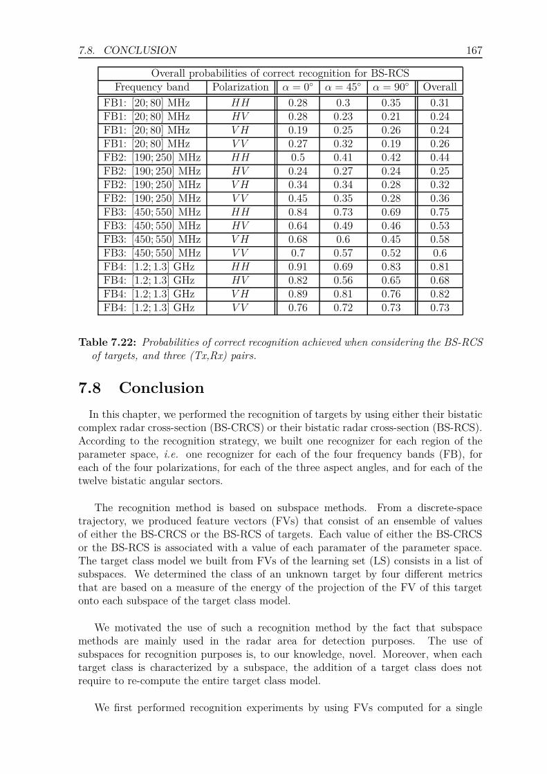
7.8. CONCLUSION 167

Overall probabilities of correct recognition for BS-RCSFrequency band Polarization α = 0◦ α = 45◦ α = 90◦ Overall

FB1: [20; 80] MHz HH 0.28 0.3 0.35 0.31FB1: [20; 80] MHz HV 0.28 0.23 0.21 0.24FB1: [20; 80] MHz V H 0.19 0.25 0.26 0.24FB1: [20; 80] MHz V V 0.27 0.32 0.19 0.26FB2: [190; 250] MHz HH 0.5 0.41 0.42 0.44FB2: [190; 250] MHz HV 0.24 0.27 0.24 0.25FB2: [190; 250] MHz V H 0.34 0.34 0.28 0.32FB2: [190; 250] MHz V V 0.45 0.35 0.28 0.36FB3: [450; 550] MHz HH 0.84 0.73 0.69 0.75FB3: [450; 550] MHz HV 0.64 0.49 0.46 0.53FB3: [450; 550] MHz V H 0.68 0.6 0.45 0.58FB3: [450; 550] MHz V V 0.7 0.57 0.52 0.6FB4: [1.2; 1.3] GHz HH 0.91 0.69 0.83 0.81FB4: [1.2; 1.3] GHz HV 0.82 0.56 0.65 0.68FB4: [1.2; 1.3] GHz V H 0.89 0.81 0.76 0.82FB4: [1.2; 1.3] GHz V V 0.76 0.72 0.73 0.73

Table 7.22: Probabilities of correct recognition achieved when considering the BS-RCSof targets, and three (Tx,Rx) pairs.

7.8 Conclusion

In this chapter, we performed the recognition of targets by using either their bistaticcomplex radar cross-section (BS-CRCS) or their bistatic radar cross-section (BS-RCS).According to the recognition strategy, we built one recognizer for each region of theparameter space, i.e. one recognizer for each of the four frequency bands (FB), foreach of the four polarizations, for each of the three aspect angles, and for each of thetwelve bistatic angular sectors.

The recognition method is based on subspace methods. From a discrete-spacetrajectory, we produced feature vectors (FVs) that consist of an ensemble of valuesof either the BS-CRCS or the BS-RCS of targets. Each value of either the BS-CRCSor the BS-RCS is associated with a value of each paramater of the parameter space.The target class model we built from FVs of the learning set (LS) consists in a list ofsubspaces. We determined the class of an unknown target by four different metricsthat are based on a measure of the energy of the projection of the FV of this targetonto each subspace of the target class model.

We motivated the use of such a recognition method by the fact that subspacemethods are mainly used in the radar area for detection purposes. The use ofsubspaces for recognition purposes is, to our knowledge, novel. Moreover, when eachtarget class is characterized by a subspace, the addition of a target class does notrequire to re-compute the entire target class model.

We first performed recognition experiments by using FVs computed for a single

168 7.8. CONCLUSION

(Tx,Rx) pair. We successively used FVs consisting of the BS-CRCS and of the BS-RCS.The recognition results show that an overall probability of correct recognition of 0.93can be achieved for a single (Tx,Rx) pair operating at a frequency between 1.2 GHzand 1.3 GHz. The achieved probability of correct recognition increases with frequency.The probability of correct recognition is sensitive to the aspect angle α, but not to thebistatic angle β. The probability of correct recognition also varies according to thepolarization used, HH being the best polarization for the targets considered. Thiscan be intuitively understood by the fact that the shapes of the different targets differmore according to their horizontal planes than their vertical planes. We also showedthat recognizing targets by using their BS-CRCS gives better results than by usingtheir BS-RCS.

We then performed recognition experiments by using FVs computed for three(Tx,Rx) pairs. We successively used FVs consisting of the BS-CRCS and of theBS-RCS. An overall probability of correct recognition of 0.98 can be achieved atthe highest frequency band considered, and at polarization HH , when consideringthe BS-CRCS of targets. As for a single (Tx,Rx) pair, the probability of correctrecognition increases with frequency, and varies according to polarization, HH beingthe best polarization. The recognizer is less sensitive to the aspect angle α whenconsidering three (Tx,Rx) pairs.

Compared to the recognition of targets by using their radar images (Chapter 6),we need fewer transmitters and receivers to recognize targets. Indeed, while we need2D diversity to compute radar images of targets, we simply need a 1D diversity tocompute FVs of either BS-CRCS or BS-RCS.

In comparison to the probabilities of correct recognition achieved for the recognitionof targets by using their radar images, the probabilities of correct recognition achievedfor a single (Tx,Rx) pair are of the same order for the first frequency band ([20; 80]MHz), and are lower for the three other frequency bands. This can be explained bythe fact that the images contain much more information than the FVs of BS-CRCS orBS-RCS. When using multiple (Tx,Rx) pairs, i.e. three in the experiments performedhere, the probability of correct recognition rises by about 10%, thus approachingthe probabilities of correct recognition achieved when dealing with radar images oftargets. Increasing the number of (Tx,Rx) pairs thus increases the probability ofcorrect recognition.

The recognition results we obtained in this chapter showed experimentally thatthe recognition of targets by using either their BS-CRCS or their BS-RCS, withoutreconstructing their radar images, is efficient, especially when considering multiple(Tx,Rx) pairs. In Chapter 8, we apply this recognition method on experimentally-acquired, real-life BS-RCS of airplanes.

Chapter 8

Recognition of targetsby using theirexperimentally-acquired, real-lifebistatic RCS

Contents8.1 Motivation . . . . . . . . . . . . . . . . . . . . . . . . . . . . 170

8.2 Block diagram of the ATR system . . . . . . . . . . . . . . 171

8.3 Detection, discrimination, and pre-classification . . . . . . 171

8.4 Classes of targets . . . . . . . . . . . . . . . . . . . . . . . . 172

8.4.1 Types of detected airplanes . . . . . . . . . . . . . . . . . . . 172

8.4.2 Grouping of targets into classes . . . . . . . . . . . . . . . . . 174

8.5 Scene parameters . . . . . . . . . . . . . . . . . . . . . . . . 176

8.6 Extraction of the BS-RCS . . . . . . . . . . . . . . . . . . . 176

8.6.1 Extraction of the BS-RCS from real-life data . . . . . . . . . 176

8.6.2 Generation of the BS-RCS from a simple model . . . . . . . . 180

8.7 Recognition stage . . . . . . . . . . . . . . . . . . . . . . . . 180

8.8 Experimental setup . . . . . . . . . . . . . . . . . . . . . . . 181

8.8.1 Testbed . . . . . . . . . . . . . . . . . . . . . . . . . . . . . . 181

8.8.2 The VOR as a simple illuminator of opportunity . . . . . . . 181

8.8.3 Collecting the received signals by an SDR receiver . . . . . . 183

8.8.4 Digital processing of received signals . . . . . . . . . . . . . . 183

8.9 Data collected and examples of received signals . . . . . . 184

8.9.1 Data available for our recognition experiments . . . . . . . . 184

8.9.2 Received ADS-B data . . . . . . . . . . . . . . . . . . . . . . 185

8.9.3 Spectrograms . . . . . . . . . . . . . . . . . . . . . . . . . . . 185

8.9.4 Signal-to-noise-ratios . . . . . . . . . . . . . . . . . . . . . . . 187

8.9.5 Variations of the BS-RCS as a function of time . . . . . . . . 189

169

170 8.1. MOTIVATION

8.9.6 Distributions of the BS-RCS in (α, β) plane . . . . . . . . . . 189

8.10 Errors on position, bistatic angle, and BS-RCS . . . . . . 193

8.10.1 Error on the position of a target . . . . . . . . . . . . . . . . 193

8.10.2 Influence of the error in position on the bistatic RCS . . . . . 193

8.10.3 Reasons for using the BS-RCS instead of the BS-CRCS . . . 196

8.11 Recognition experiments performed . . . . . . . . . . . . . 196

8.11.1 Amount of data . . . . . . . . . . . . . . . . . . . . . . . . . . 197

8.11.2 Statistics of the feature vectors and brief analysis thereof . . 202

8.11.3 Recognition results for the three-class experiment . . . . . . . 202

8.11.4 Recognition results for all four recognition experiments . . . 208

8.12 Conclusion . . . . . . . . . . . . . . . . . . . . . . . . . . . . 208

In this chapter, we perform the recognition of air targets by using their bistaticradar cross-section (BS-RCS) that we compute from real-life signals acquired usinga passive radar testbed. Section 8.1 describes the motivation for this problem. Sec-tion 8.2 presents the block diagram of the implemented automatic target recognition(ATR) system. Section 8.3 presents the detection and discrimination stages of thisATR system. Section 8.4 discusses the grouping of the types of detected airplanesinto classes. Section 8.5 describes the computation of the scene geometry. Section 8.6presents the extraction of the BS-RCS of detected airplanes, and the generation of theBS-RCS for small airplanes, which we cannot detect. Section 8.7 presents the recogni-tion stage of the ATR system. Section 8.8 presents the experimental setup that we useto collect real-life signals. Section 8.9 presents the collected data, and shows exampleof received signals. Section 8.10 describes the error on the position of the airplanes,its influence on the value of the BS-RCS, and the reasons for using the BS-RCS of theairplanes instead of their bistatic complex radar cross-section (BS-CRCS). Section 8.11presents the recognition experiments we perform and the achieved probabilities of cor-rect recognition. Section 8.12 concludes.

8.1 Motivation for the recognition of targets by us-

ing their real-life bistatic RCSs

In Chapter 7, we performed the recognition of (air) targets by using either theirbistatic complex radar cross-section (BS-CRCS) or their bistatic radar cross-section(BS-RCS). The BS-CRCS and the BS-RCS of the targets of interest were extractedfrom signals transmitted and received in an anechoic chamber. We now plan to testthe recognizer developed in Chapter 7 on BS-RCS of (air) targets computed fromreal-life signals, acquired in the real, outdoor world. In this chapter, we deal withthe recognition of targets by using their BS-RCS, which are extracted from real-lifepassive bistatic radar signals.

To demonstrate the validity of our approach, we built a passive-radar-systemtestbed consisting of one transmitter (Tx) of opportunity and one receiver (Rx). Wedeployed the testbed - produced by the SONDRA lab of SUPELEC - in the vicinityof Orly Airport, near Paris, France. We collected the data almost continuously for

8.2. BLOCK DIAGRAM OF THE ATR SYSTEM 171

ten days, which allows us to perform recognition experiments involving three classes ofairplanes. (The data for the last class were generated by simulation.)

8.2 Block diagram of the automatic target recogni-

tion system

Figure 8.1 shows the block diagram of the automatic target recognition (ATR)system. Since we are in a real, outdoor configuration, we first detect targets in thedetection stage. We then determine whether the detected targets are of interestor not in the discrimination and pre-classification stage. These detection anddiscrimination/pre-classification stages are the only differences with the ATR systemthat is discussed in Chapter 7. For each target of interest, we extract its bistaticradar cross-section (BS-RCS) from (1) the signal transmitted by an illuminator ofopportunity and scattered on the target, and (2) the scene parameters, which consistin the scene geometry, the polarizations of the Tx and the Rx, and the frequency ofthe Tx. We assume that the scene parameters are known.

Figure 8.1: Block diagram of our ATR system using real-life bistatic radar cross-sections of air targets.

For a particular detected target, the scattered signals belong to either the learningset (LS) or the test set (TS). The LS is used to generate the target class model, whilethe TS is used to evaluate the performance of the target class model by assigning aclass to each object of the TS.

8.3 Detection, discrimination, and pre-

classification

We must first detect targets, one at a time. Among the signals scattered by targets,we must discriminate whether a scattered signal corresponds to a target of interest tous. We define a target of interest as being the air target that we detected. For boththe detection and the discrimination (and pre-classification), we use the automaticdependent surveillance - broadcast (ADS-B) signals that are sent by airplanes followingan interrogation.

As described in Chapter 1, secondary surveillance radars (SSRs), in S-mode, sendinterrogation signals to the airplanes, on request from the control tower. The airplane

172 8.4. CLASSES OF TARGETS

transponder transmits omnidirectional (DPSK) signals at 1090 MHz. ADS-B receiverscollect such signals. In our testbed, we detect airplanes from the analysis of ADS-Bsignals. In an operational system, the detection of an air target would be performedby a conventional moving target detector (MTD) radar, such as an airport primaryradar.

ADS-B signals provide the International Civil Aviation Organization (ICAO) code(such as AFR for Air France) and the callsign (such as AFR123) of the detectedairplane. By interrogating an Internet database such as [67], we can determine thetype of airplane we detect. We use this information to define the different classes ofairplanes (8.4).

We discriminate between targets of interest and other targets in two ways. First, adetected target is thus necessarily an airplane, since only airplanes send ADS-B signals.Second, in order to discriminate between the signals scattered by different airplanesthat might be in the vicinity of the ground ADS-B receiver at the same time, we usethe position information contained in ADS-B signals to compute the Doppler shift ofthe detected airplane. Therefore, by using a Doppler filter, we select the part of thereceived signal that corresponds to the signal scattered by the appropriate airplane, asshown in Fig. 8.2.

f

t

Signal scattered

Direct-path signalDoppler filter

by airplane 1 Signal scatteredby airplane 2

Figure 8.2: Illustration of the Doppler filter applied to select the signal scattered byairplane 1 when two airplanes are in the vicinity of the passive radar system at thesame time.

8.4 Classes of targets

In this section, we present the types of airplanes that we detected during the mea-surement campaign. We then discuss the grouping of airplanes into classes.

8.4.1 Types of detected airplanes

We detected a total of 1329 airplanes during the measurement campaign. We listthe 32 different types of airplanes per type of airplane family in Table 8.1.

8.4. CLASSES OF TARGETS 173

Family Number of observations Type Number of observationsA300 4 A30B 4

A320 661

A318 6A319 235A320 308A321 112

A330 156A332 79A333 77

A340 47A342 1A343 45A346 1

B737 206

B733 9B734 2B735 3B736 4B737 13B738 175

B747 53 B744 53

B757 18B752 11B753 7

B767 70B762 8B763 54B764 8

B777 99

B772 35B773 55B77F 2B77L 1B77W 6

Embraer 190 3 E190 3Avro RJ85 5 RJ85 5Avro RJ100 1 RJ1H 1Falcon FA10 1 FA10 1Fokker F100 1 F100 1Unidentified 6

Table 8.1: List of the types and families of airplanes we detected during the measure-ment campaign.

174 8.4. CLASSES OF TARGETS

We define the classes of airplanes according to the physical characteristics of theseairplanes. We thus describe the characteristics of the different airplanes we detected inTables 8.2, 8.3, 8.4, 8.5, and 8.6. For each type of airplane, we show its length, height,wingspan, wing area, wing position, fuselage width, and number of engines.

Type of Plane A300 A310 A318 A319Length [m] 54.10 46.66 34.10 33.84Height [m] 16.5 15.8 12.51 11.76

Wing span [m] 44.84 43.89 34.10 34.10Wing area [m2] 260.0 219.0 122.0 122.4Wing position low low low low

Fuselage width [m] 5.64 5.64 3.95 3.95Number of engines 2 2 2 2

Table 8.2: Characteristics of the Airbus airplanes, from A300 to A319 [2].

Type of Plane A320 A321 A330 A340Length [m] 37.57 44.51 63.69 67.93Height [m] 11.0 11.76 16.83 17.28

Wing span [m] 34.10 34.10 60.30 63.45Wing area [m2] 122.6 123.0 363.1 363.1Wing position low low low low

Fuselage width [m] 3.95 3.95 5.64 5.64Number of engines 2 2 2 4

Table 8.3: Characteristics of the Airbus airplanes, from A320 to A340 [2].

Type of Plane BAe Avro RJ85 BAe Avro RJ100Length [m] 28.60 26.34Height [m] 8.59 8.59

Wing span [m] 26.34 26.34Wing area [m2] 77.3 77.3Wing position high high

Fuselage width [m] 3.56 3.56Number of engines 4 4

Table 8.4: Characteristics of the British Aerospace airplanes RJ85 and RJ100 [90].

8.4.2 Grouping of targets into classes

Tables 8.2, 8.3, 8.4, 8.5, and 8.6 show that the size, and thus, the characteristicdimension of the (detected) airplanes vary from 26 m to 74 m. At the frequencyof the transmitter of opportunity (further discussed below) of 114.7 MHz, with

8.4. CLASSES OF TARGETS 175

Type of Plane B737 B747 B757 B767-400 B777-300Length [m] 42.1 70.66 46.7 61.3 73.9Height [m] 12.6 19.41 6.45 16.8 18.5

Wing span [m] 35.8 64.44 38.05 51.9 60.9Wing area [m2] 91.1 511.0 181.25 - 427.8Wing position low low low low low

Fuselage width [m] 5.7 6.50 3.76 9.3 6.50Number of engines 2 4 2 2 2

Table 8.5: Characteristics of the Boeing airplanes [19].

Type of Plane Embraer E190 Falcon 10 Fokker 100Length [m] 36.24 13.86 35.53Height [m] 10.28 4.61 8.50

Wing span [m] 28.72 13.08 28.08Wing area [m2] 92.5 24.1 93.5Wing position low low low

Fuselage width [m] 3.01 - 3.08Number of engines 2 2 2

Table 8.6: Characteristics of various other airplanes [90].

corresponding wavelength λ of 2.62 m, the key ratio λ/D varies from 0.035 to 0.1.We saw in Chapter 3 that, for such ratios, the scattering mechanisms are mainly afunction of the shape of the airplanes.

The tables show that all detected commercial airplanes have essentially the sameshapes, except for the overall size and the number of engines. It thus makes sense todefine two classes for commercial airplanes: large-size airplane with four engines andmid-size airplanes with two engines.

Table 8.1 does not include smaller airplanes, such as private planes, because mostof the smaller airplanes do not have ADS-B, the result being that we were unable todetect them. However, it makes sense to define a third class to include these smallerairplanes. We thus decide to define the following three classes based upon the overallsize S [m] (the largest of wing span and fuselage length) and the number of engines

• S < 20 : class of small-size airplanes

• 20 ≤ S < 30: no class defined

• 30 ≤ S < 40 and 2 engines: class of mid-size airplanes

• 40 ≤ S < 50: no class defined

• 50 ≤ S and 2 engines: no class defined

• 50 ≤ S and 4 four engines: class of large-size airplanes.

176 8.5. SCENE PARAMETERS

8.5 Scene parameters

The scene parameters, i.e. the positions of the transmitter (Tx) and the receiver(Rx), the position of a detected airplane throughout its trajectory, the polarizations ofthe Tx and the Rx, and the frequency of the Tx, are an input of the automatic targetrecognition (ATR) system. The positions of both the Tx and the Rx are known sincethey are fixed. The polarizations of the Tx and the Rx, and the frequency of the Txare known by construction of the passive radar testbed.

In order to compute the position of a detected airplane, we use the informationsent via the ADS-B signals. In an operational system, the position of a detectedairplane would be given by a radar such as an airport primary surveillance radar.

The information sent by the ADS-B system aboard an airplane (upon interrogation)contains the position of the airplane. Each position is provided as latitude, longitude,and barometric altitude, and is encoded according to the Compact Position Reporting(CPR) format. We use the position of the airplane over time to compute the Dopplershift of the signal scattered by this airplane, as explained in Section 8.3. We alsouse the position of the airplane to compute its bistatic radar cross-section (BS-RCS),aspect angle α, and bistatic angle β, which are the parameters of the parameter space(Section 6.2).

We also know the polarization and the frequency of the Tx, and the polarization ofthe Rx.

8.6 Extraction of the bistatic RCS for the three

airplane classes of interest

We describe our method for the extraction of the bistatic radar cross-section(BS-RCS) from real-life data for the mid-size and large-size airplanes. Since we couldnot detect small-size airplanes, we generate the BS-RCS of small-size airplanes from asimple, adjustable model.

8.6.1 Extraction of the bistatic RCS from real-life data for

mid-size and large-size airplane classes.

Consider the bistatic (BS) configuration shown in Fig. 8.3 for a single (Tx,Rx) pair.The transmitter (Tx) is located at T and the receiver (Rx) at R. The object of interestis located at S. We assume that the geometry is known. The Tx sends out a transmitsignal - which can be viewed as being a continuous-wave (CW) signal - and the Rxreceives the sum of the direct signal (from R) and the scattered signal (from S) [186].However, as explained later, our technique requires that we are able to separate thesetwo signals.

These signals differ by their different arrival times, but the difference betweenthese signals is too short to allow one to separate the signals in the time domain, thereason for this being the sampling frequency of 48 kHz. The different arrival times

8.6. EXTRACTION OF THE BS-RCS 177

GTRT

R

S

RTS RRS

RTR

Scatteringpath

Transmitpath

Direct path

PRD

PRS

(Object)

(Tx)

(Rx)b

b GTS

LFS orLNLOS

b

bGRS

GRT

bbb

b

b

β

Figure 8.3: Bistatic (BS) radar configuration corresponding to one (Tx,Rx) pair look-ing at one object. T , R, and S are the positions of the Tx, Rx, and object, respec-tively. The figure shows the antenna beampatterns for the Tx and Rx. It also showsthe transmit path TS, the scattering path SR, and the direct path TR, along each ofwhich the corresponding signal travels. The various parameters shown are discussedin the text. The figure is used as a support to explain how the BS-RCS of the objectis obtained from the signal received at R, which is the sum of the direct signal andthe scattered signal (if any).

could be computed if the sampling frequency was much higher. However, the motionof the object induces a Doppler shift in the scattered signal received from S, and thisleads to both signals being generally (but not always) well separated in frequency. Theonly hope is thus to separate the two signals of interest in the frequency domain. Inthe analysis below, we assume that the direct and scattered signals can be separated.This allows us to get their respective power.

We denote by PT the power transmitted (by the Tx). We denote by PRX the powerreceived (by the Rx), with X replaced by D for the direct path, and by S for thescattering path.

The scattered power PRS received from S is given by the BS radar equation [224],expressed in natural units (i.e. Watts),

PRS =PTGTSGRSλ

2σ

(4π)3R2TSR

2RS

, (8.1)

where the GXS’s and RXS’s are the antenna gains and the ranges shown in Fig. 8.3,λ the wavelength of the transmitted signal, and σ the BS-RCS of the object for thegiven configuration and object orientation. More specifically, GTS is the gain of theTx antenna in the direction of S, and GRS is the combined gain of the Rx antenna inthe direction of S and of the gain of the Rx chain.

The power PRD received directly from T is given by the link budget equation [99],

178 8.6. EXTRACTION OF THE BS-RCS

expressed in natural units,

PRD =PTGTRGRT

L, (8.2)

where GTR and GRT are the antenna gains shown in Fig. 8.3, and L the propagationloss, which is further discussed later.

The desired BS-RCS σ is directly obtained from the ratio

PRSPRD

=GTSGRSλ

2σL

(4π)3R2TSR

2RSGTRGRT

. (8.3)

One finds

σ =PRSPRD

GTRGRT

GTSGRS

(4π)3R2TSR

2RS

λ2L. (8.4)

Observe that PT , which is unknown (since the Tx is an illuminator of opportunity),does not appear in the above equation for σ.

By introducing the gain-ratio parameter G = GTR/GTS, we can rewrite the lastequation as

σ =PRSPRD

GRT

GRS

G(4π)3R2

TSR2RS

λ2L. (8.5)

On the right-hand side of this equation, the two powers PRS and PRD can be measuredfrom the received signals; the ranges RTS and RRS can easily be found since theconfiguration geometry is known; the gains GRT and GRS of the Rx antenna can beobtained from the configuration geometry and the Rx antenna beampattern (and thus,for each position S of the object); and, of course, λ is known. Since the beampatternof the Tx antenna is unknown, the gains of the transmitted signals GTR and GTS areunknown. The last quantity to be discussed is the loss L.

If the direct path TR between T and R is unobstructed, i.e. "line of sight (LOS)",also called "free space (FS)", then the corresponding loss L is denoted by LLOS, or LFS ,and is given by [99]

LLOS =(

4πRTR

λ

)2

, (8.6)

where λ = c/f is the wavelength, and RTR the distance from T to R (in km).

If the path TR is obstructed, i.e. "non-LOS (NLOS)", then the corresponding lossis denoted by LNLOS, and is given by

LNLOS = LLOSLTER, (8.7)

and, in dBs, byLNLOS = LLOS + LTER [dB], (8.8)

where LTER is the additional loss due to the terrain and other obstructions, referredto here as the terrain loss.

The terrain loss LTER is unknown. However, it is important to observe that, forour configuration geometry, LTER is approximately constant. While we could try to

8.6. EXTRACTION OF THE BS-RCS 179

estimate LTER, here we simply use LLOS in Eq. (8.5), which yields a "biased" BS-RCS,denoted by σ′, and given by

σ′ = KG

LLOS, (8.9)

where

K =PRSPRD

GRT

GRS

(4π)3R2TSR

2RS

λ2. (8.10)

This biased BS-RCS σ′ is related to the true BS-RCS σ = KG/LNLOS via

σ′ = GLNLOSLLOS

σ = GLTER σ, (8.11)

and, in dBs, viaσ′ = σ +G+ LTER [dB]. (8.12)

More generally, the value σ′ obtained for the BS-RCS is related to the true BS-RCSσ via σ′ = σ + ∆σ [dB], where ∆σ includes the terrain loss, the non-omnidirectionalbeampattern of the Tx antenna, and other systematic errors that are assumed to remainquasi constant during the measurement campaign, as shown in Fig. 8.4. Our recognizeris trained and tested on the biased σ′, rather than on the true σ. However, the biasedBS-RCS will, in the sequel, still be denoted by σ, rather than by σ′.

−180 −170 −160 −150 −140 −130 −120 −110 −100 −900

2000

4000

6000

8000

10000

12000

Power [dB]

Num

ber

of o

ccur

ence

s

Histogram of power of received direct signal

Figure 8.4: Histogram of the power of the received direct signal. One clearly sees thatthe terrain loss and other systematic errors are quasi constant through the measure-ment campaign, thus validating the approach for the computation of the BS-RCS.

180 8.7. RECOGNITION STAGE

8.6.2 Generation of the bistatic RCS from a simple, adjustablemodel for small-size airplane class

Since we could not detect small-size airplanes, we produced BS-RCS data for thesmall-size airplane class by using a simple model consisting of one wire for the bodyand one wire for each wing (Fig. 8.5).

φ2φ3

L2

L3

L1

Figure 8.5: Model for the airplanes in the small-size airplane class. This simplemodel consists of three wires, one for the body and one for each wing.

The BS-RCS σ corresponding to a model consisting of N wires of length Li andangle φi is computed according to the following formula,

σ =N∑

i=1

Li sinc(Xi), (8.13)

where

Xi =2πLiλ

sinαT + αR + φi

2cos

β

2, (8.14)

and where αT and αR are the angles between the pointing direction of the airplaneand TS and SR, respectively (Fig. 6.4).

To position and orient the small-size airplanes, we use the information recordedfor all real mid-size airplanes observed. Therefore, we have as many samples for thesmall-size airplanes as we have for the mid-size airplanes. To provide size diversity, thelength of each model wire was varied randomly in an interval centered on 4 m for thebody, and 2 m for each wing, the width of the intervals being 20% of the center value.

8.7 Recognition stage

We use the same recognizer that we used in Chapter 7. For each tile of the parameterspace (α, β), we build one recognizer. Each of the three target classes is characterizedby a subspace. The subspaces are formed from feature vectors (FVs) exactly asdescribed in Section 7.4.2. We produce FVs exactly as in Section 7.3. Each FV is aone-dimensional array of N bistatic radar cross-section (BS-RCS) values expressed indecibel units. Each BS-RCS value is associated to a point in the parameter space.We emphasize that, for a given airplane, and thus a given trajectory, we can produceseveral FVs that correspond to several tiles of the parameter space.

8.8. EXPERIMENTAL SETUP 181

The class assigned to an unknown target, characterized by its FV, is decided basedon the projection and metrics defined in Sections 7.5.1 and 7.5.2, respectively.

We separate the detected airplanes of each of the three classes into a learning set(LS) and a test set (TS). For each class of airplanes, the first third of the total numberof detected airplanes (and thus their corresponding trajectories and their correspondingBS-RCS values) is used for the LS, and the last two thirds for the TS.

8.8 Experimental setup

Our goal is to perform the recognition of airplanes of three categories, i.e. large-sizeairplanes (e.g. A343), mid-size airplanes (e.g. A319), and small-size airplanes (e.g.private planes and UAVs), by using the bistatic radar cross-section (BS-RCS) of theseairplanes. We describe the experimental setup we deployed to get real-life data for thelarge-size and mid-size airplanes.

8.8.1 Testbed

The passive-radar testbed was designed and put together by Sylvain Azarian fromSUPELEC/SONDRA, and then deployed in the vicinity of Orly Airport, south ofParis, France (Fig. 8.6). This allowed us to observe airplanes in approach for landing,climbing after take-off, or following airways.

The testbed ends up consisting of a single (Tx,Rx) pair. The transmitter (Tx) ofopportunity is the VOR (VHF Omni Range) Tx located at Rambouillet, with identifierRMB, and operating on frequency of 114.7 MHz and vertical polarization (Fig. 8.6). AVOR is a navigation aid widely used in aviation. The choice of such an illuminator ofopportunity is discussed below. The receiver (Rx) is based on a software-defined radio(SDR) [135] designed at SONDRA lab. The Rx is located at the point marked "Rx" inFig. 8.6, and operates on vertical polarization. The distance between the Tx and theRx is of 15.5 km. To obtain the necessary information about each observed airplane,i.e. identity (such as callsign) and position, we use an ADS-B receiver co-located withthe SDR-based Rx.

We planned to use, as a second Tx of opportunity, the VOR located at Epernon(EPR, 115.65 MHz), but the corresponding signal-to-noise ratio (SNR) at our Rxproved to be too small to be usable.

Using this experimental setup, we recorded the trajectories of 1329 airplanes of 32different types (as defined according to [67]) of airplanes listed in Section 8.4, over aperiod of ten days.

8.8.2 The VOR as a simple illuminator of opportunity

We define the following requirements for the choice of the transmitter of opportunityof our passive-radar-based system:

182 8.8. EXPERIMENTAL SETUP

u

Orly Airport

RMB VOREPR VOR

Rx

Illustrative trajectories

Paris

ut

u

u

15.5 km10 km(Tx)

RambouilletEpernon Tx

SDR, ADS-BRambouillet

Figure 8.6: Schematic of the Orly Airport area showing the location of the Tx and Rxused in our passive radar testbed. The Tx is the RMB VOR located at Rambouillet.The Rx - consisting of a software-defined radio (SDR) - is located at a private home.The figure also shows the EPR VOR of Epernon, which we tried to use, but the SNRof which was too small to be usable. The figure also shows samples of four differentairplanes trajectories (dashed lines).

• The transmitting power shall be constant through time since it is used in thecomputation of the BS-RCS. The knowledge of the transmitting power is notrequired (Section 8.6)

• The transmitted signal shall not be modulated, in order to keep the systemsimple. The ideal case is that of a carrier frequency.

• The transmitter shall operate on low frequencies, i.e. on frequencies smaller than1 GHz. The operating frequency shall remain constant through time.

• The beampattern of the transmitting antenna shall not be only directed towardsthe ground, since we want the transmitted signal to be scattered by airplanes.

The VHF Omni-Range (VOR) is a quasi-ideal transmitter of opportunity, sinceit satisfies all of these constraints. Figure 8.7 shows the spectrum of the signaltransmitted by a VOR. The spectrum of the signal of the VOR consists of one humpcentered at the carrier frequency fc corresponding to audio information (such asthe VOR callsign), one "sinusoid" (or at least one very narrow-band signal) at thefrequency of fc + 9, 960 Hz, called the subcarrier, and two weaker sinusoids located30 Hz away on each side of the subcarrier, and due to the physical rotation of theVOR antenna. The subcarrier is important because it is well separated from theother frequency components and is thus an almost ideal monochromatic illuminator ofopportunity.

8.8. EXPERIMENTAL SETUP 183

Figure 8.7: Idealized spectrum of a VOR. The "sinusoid" corresponding to the sub-carrier is the effective signal used as an illuminator of opportunity.

The chosen illuminator of opportunity is the VOR transmitter located at Ram-bouillet, with callsign RMB, and operating on 114.7 MHz. The spectrogram of a directsignal received from the VOR is shown in Section 8.9.

8.8.3 Collecting the direct and scattered signals by an SDRreceiver

As shown in Section 8.6, we have to collect (1) the direct signal, which is thesignal transmitted by the VOR and directly (i.e. without any scattering) collectedby the Rx, and (2) the scattered signal, which is the signal transmitted by the VOR,scattered by the target, and collected by the Rx.

We collect these two signals by using a software-defined radio (SDR) re-ceiver [3, 99, 135]. The role of the SDR is to convert the radiofrequency (RF) signalsto their baseband in-phase and quadrature components. Figure 8.8 shows a schematicof the SDR used in our experiments. The SDR converts the RF signals to basebandby using a cascade of three filters and three mixers.

The input RF signal is first passed through an 8th-order low-pass filter with cutofffrequency of 200 MHz, and then through a band-pass filter centered on 115 MHz (aboutthe frequency of the VOR). The resulting signal is mixed to an intermediate frequency(IF) fIF = 22.94 MHz. The resulting signal is passed through a band-pass filtercentered on fIF . The resulting IF signal is mixed to produce the baseband in-phaseand quadrature components, I(t) and Q(t), respectively.

8.8.4 Digital processing of received signals

The I(t) and Q(t) components are digitized by using a computer sound card, to getthe digital in-phase and quadrature components, I[n] and Q[n], respectively. A setupprocedure is performed before acquisition to compensate the I/Q mismatch caused bydifferent gains and delays in the left and right audio channel.

184 8.9. DATA COLLECTED AND EXAMPLES OF RECEIVED SIGNALS

Figure 8.8: Conversion of the RF input signals to baseband performed by the SDRreceiver. The input signal is first filtered twice and then successively converted fromRF to IF and from IF to baseband.

The Fast Fourier Transform (FFTs) is applied to successive segments of the complexsequence I[n] + jQ[n] to obtain the spectrum of the received signal. A spectrogram,which shows the variation of the spectrum as a function of time, of the received signalis obtained by repeating the same operations at successive time instants. Examples ofspectrograms are shown in Section 8.9.

8.9 Data collected and examples of received signals

In this section, we present the data available for our recognition experiments. Wealso show examples of data computed from the received ADS-B signals. We then showexamples of spectrograms of signals received by the SDR receiver. We then show thesignal-to-noise ratios of both the direct and the scattered signals, and an example of thevariations of the bistatic radar cross-section (BS-RCS) as a function of time. Finally,we last show, for each class of airplanes, the distributions of the BS-RCS in the (α, β)parameter space.

8.9.1 Data available for our recognition experiments

The first two sections of Table 8.7 summarize the part of the real data we collectedwith our passive radar testbed during the measurement campaign that lasted tendays, and that we use for our recognition experiments. The table only shows the typesof airplanes for which a significant amount of data is available. Airplanes are dividedinto the three classes defined earlier. The first two consist of real data. For each typeof airplane (in each class), the table gives the number of trajectories observed and thetotal number of samples obtained, for both the learning set (LS) and the test set (TS).

8.9. DATA COLLECTED AND EXAMPLES OF RECEIVED SIGNALS 185

The number of trajectories is also the number of times an airplane of a given type wastracked. The number of samples is also the number of BS-RCS values available for alltrajectories. The last section of Table 8.7 summarizes the synthetic data produced.

Learning set Test setType of air-plane

Number oftrajectories

Number ofsamples

Number oftrajectories

Number ofsamples

Large-size airplanes - Real dataA342 1 11 0 0A343 15 973 30 1680A346 1 8 0 0Total 17 992 30 1680

Mid-size airplanes - Real dataA318 2 56 4 159A319 78 3316 157 6208A320 102 5472 206 10530Total 182 8844 367 16897

Small-size airplanes - Synthetic dataMisc. 182 8546 367 17195

Total (all) 381 18382 764 35772

Table 8.7: Data available for our recognition experiments. The types of airplanes areorganized in the three categories of large-size, mid-size, and small-size airplanes.The first two categories contain real data collected with our passive radar testbed.The last one contains synthetic data we produced. The table gives the number oftrajectories and samples available for each type of airplane.

8.9.2 Received ADS-B data

We compute the trajectory of airplanes from the positions received by ADS-B signals.Figure 8.9 shows the reconstructed trajectory of an airplane. We also compute thebistatic angle and the (smoothed) Doppler shift as a function of time, i.e. essentiallyalong the airplane trajectory, shown in Figs. 8.10 and 8.11, respectively. The Dopplershift is smoothed by using a low-pass filter. Indeed, since commercial airplanes flyaccording to simple trajectories such as straight lines, the Doppler shift varies smoothlyalong the airplane trajectory, i.e. from one time instant to the next.

8.9.3 Spectrograms

Figure 8.12 shows a spectrogram of the signal received by our (SDR) Rx tuned to thefrequency of the RMB VOR, this in the absence of any airplane in the field of view. Thespectrogram thus corresponds to the direct signal only. By definition, the spectrogramshows the variation of the power received as a function of frequency and time. Thefigure also shows a cut at a given time, i.e. the spectrum of the signal at that time.

186 8.9. DATA COLLECTED AND EXAMPLES OF RECEIVED SIGNALS

−1−0.5

00.5

11.5

x 104

−5000

0

5000

100000

1000

2000

3000

4000

5000

Airplane trajectory

x−axis [m]

Transmitter position

Receiver position

Reconstructed trajectory of an airplane

y−axis [m]

z−ax

is [m

]

Figure 8.9: Reconstructed trajectory of an airplane. The locations of the Tx and theRx are also shown.

0 5 10 15 20 25 30 35 40 45 5030

40

50

60

70

80

90

100

110

120

130Bistatic angle β as a function of time

Time index

Bis

tatic

ang

le β

[°]

Figure 8.10: Variation of the bistatic angle β as a function of time, i.e. essentiallyalong the trajectory of an airplane. (Same as Fig. 4.6.)

8.9. DATA COLLECTED AND EXAMPLES OF RECEIVED SIGNALS 187

0 5 10 15 20 25 30 35 40 45 50−500

−400

−300

−200

−100

0

100

Time index

Dop

pler

shi

ft [H

z]

Doppler shift as a function of time

DopplerDoppler smoothed

Figure 8.11: Variation of the Doppler shift as a function of time, i.e. essentiallyalong the trajectory of an airplane.

Not surprisingly, the spectrum remains virtually the same at all times. This spec-trum can be understood in terms of the idealized spectrum of a VOR shown in Fig. 8.7.

Figure 8.13 shows a spectrogram of the signal consisting in the sum of the directsignal and the scattered signal, the latter being due to an (A319) airplane. It is clearthat the three vertical traces correspond to the direct signal received from the VOR,and that the three curved traces correspond to the scattered signal from the airplane.The "curving" is due to the time-dependent Doppler shift due to the motion of theairplane.

Spectrograms such as that of Fig. 8.13 automatically separate (at least to the eye)the direct signal and the scattered signal. At any time t, and as long as the separationin frequency is sufficient, we can easily read off the powers PRS and PRD (Fig. 8.3)that are required to compute the airplane radar cross-section (RCS) σ at this time.

8.9.4 Signal-to-noise-ratios

To read off the above powers of the direct and scattered signals, the signal-to-noiseratios (SNRs) must be sufficient. The SNR at some instant is defined as the ratio ofthe signal power to the noise power at this instant, for a given frequency bandwidth.The power of the noise is measured at any time instant by taking the mean of thepower of the received signal in zones outside that of the signal of interest, such as infrequency indices 120 to 140 in Fig. 8.13.

Figure 8.14 shows the SNR of the received direct signal from the RMB VOR as afunction of time. As expected, this SNR is relatively constant. Its value is from 40 to50 dB. Figure 8.15 shows the SNR of the scattered signal as a function of time. As

188 8.9. DATA COLLECTED AND EXAMPLES OF RECEIVED SIGNALS

Figure 8.12: Spectrogram (in "waterfall view") of the signal received in the absenceof airplanes. It thus corresponds to the spectrogram of the signal received from theRMB VOR over the direct path. The spectrogram can be interpreted with the help ofFig. 8.7.

Spectrogram

Frequency index

Tim

e in

dex

20 40 60 80 100 120 140 160 180 200

5

10

15

20

25

30

35

40

45

2

4

6

8

10

12

14

16

18

20

22

Figure 8.13: Spectrogram (in "waterfall view") of the signal received in the presenceof one airplane. The figure only shows the frequency region near the subcarrierfrequency. At most instants, one can easily distinguish between the straight tracesdue to the direct signal and the curved traces due to the scattered signal. We exploitthe separation in frequency between these two components at most instants to get thepowers required to compute the RCS values.

8.9. DATA COLLECTED AND EXAMPLES OF RECEIVED SIGNALS 189

time increases, the position and "view" of the airplane varies, resulting in variations ofits bistatic radar cross-section (BS-RCS). The observed variations in SNR with timeare directly linked to the variations in BS-RCS with time. However, the value of theSNR is almost always above 25 dB, which guarantees an accurate calculation of theBS-RCS from the measurement of the powers PRS and PRD. We were not able to usethe VOR of Epernon, France, precisely because the SNR of the received signal wastoo small. The sharp transition at the beginning of each of Figs. 8.14 and 8.15 can beignored.

0 5 10 15 20 25 30 35 40 450

10

20

30

40

50

60Signal to noise ratio as a function of time

Time index

SN

R [d

B]

Figure 8.14: Variation, as a function of time, of the signal-to-noise ratio (SNR)of the signal received in the absence of airplanes and, thus, corresponding to thedirect-signal component only.

8.9.5 Variations of the bistatic RCS as a function of time

Using the values of PRS and PRD obtained as a function of time from a spectrogramsuch as that of Fig. 8.13, one can determine, from Eq (8.5), the value of the BS-RCSas a function of time. Figure 8.16 shows an example of the variation of BS-RCS asa function of time. Once again, as time increases, the airplane moves and presentsdifferent aspect angles.

8.9.6 Distributions of the bistatic RCS in (α, β) plane

Since we know the configuration geometry at any time, we can map the mea-sured (discrete space (DS)) trajectories and corresponding BS-RCS values fromthe (x, y) plane to the (α, β) plane. The resulting distributions of BS-RCS in the(α, β) plane are illustrated in Figs. 8.17, 8.18, and 8.19 for the three classes ofairplanes. Figure 8.17 shows the 2672 real BS-RCS values corresponding to the 47

190 8.9. DATA COLLECTED AND EXAMPLES OF RECEIVED SIGNALS

0 5 10 15 20 25 30 35 40 450

10

20

30

40

50

60

70

80Signal to noise ratio as a function of time

Time index

SN

R [d

B]

Figure 8.15: Variation, as a function of time, of the signal-to-noise ratio (SNR) ofthe signal received from one airplane and, thus, corresponding to the scattered-signalcomponent only. The variations are due to the changes in aspect angle and in bistaticangle as the airplane goes by.

0 5 10 15 20 25 30 35 40 450

10

20

30

40

50

60RCS as a function of time

Time index

RC

S [d

Bsm

]

Figure 8.16: Variation, as a function of time, of the BS-RCS extracted from thereceived data, via a spectrogram, such as the one shown in Fig. 8.13.

8.9. DATA COLLECTED AND EXAMPLES OF RECEIVED SIGNALS 191

large-size airplanes observed during our measurement campaign; Fig. 8.18 showsthe 25741 real BS-RCS values corresponding to the 549 mid-size airplanes observedover this campaign; Fig. 8.19 shows the 25741 BS-RCS values produced syntheti-cally for the small-size airplanes. The various numbers just cited are those of Table 8.7.

Figure 8.17: Values of the bistatic RCS for all our (real) large-size airplanes, shownin the (α, β) plane.

The comparison of the plots of Figs. 8.17, 8.18, and 8.19 shows that the threeBS-RCS values at, or near, a given (α, β) point are generally quite different. Of course,our recognition system is designed to exploit these differences.

192 8.9. DATA COLLECTED AND EXAMPLES OF RECEIVED SIGNALS

Figure 8.18: Values of the bistatic RCS for all our (real) mid-size airplanes, shownin the (α, β) plane.

Figure 8.19: Values of the bistatic RCS for all our (synthetic) small-size airplanes,shown in the (α, β) plane.

8.10. ERRORS ON POSITION, BISTATIC ANGLE, AND BS-RCS 193

8.10 Errors on the position, the bistatic angle, and

the bistatic RCS

The data we receive from ADS-B signals in not free of errors. In this section, wefirst quantify the error on the position of the airplane. We then express the influenceof the error on the position on the values of the bistatic angle and the bistatic radarcross-section (BS-RCS). We also express the reasons for using the BS-RCS instead ofthe bistatic complex radar cross-section (BS-CRCS).

8.10.1 Error on the position of a target

As shown in Section 8.6, we compute the BS-RCS of an airplane by using the dis-tances transmitter-target (RTS) and receiver-target (RRS) and the powers of both thereceived scattered signal (PRS) and the received direct signal (PRD). Equation (8.10)is valid for any particular time instant, provided that RTS, RRS,PRD, and PRS areknown at the same particular time instant. However, there is some delay betweenthe time instant at which any ADS-B signal is sent from the plane transponder, andthe time instant at which the ADS-B signal is received (and decoded) at the ADS-Breceiver. There is also some delay for the data processing. These delays induce anerror between the computed position of the airplane and to its true position.

To compute the maximum error on the position of an airplane, we assume that themaximum speed of an aircraft is 1000 km/h, i.e. roughly 280 m/s. The position isgiven by a GPS on-board the aircraft, once every second. The accuracy of the GPS isassumed to be of 10 m. The encoding error due to the Compact Position Reportingformat (CPR) is of 5.1 m.

In the worst case, there is a delay of 1 s between the times the airplane ac-quires its position and sends it. Assuming a decoding and post-processing delay of100 ms at the receiver, the total delay is of 1.1 s between the times the airplaneacquires its position and the actual position of the airplane for which we collectthe scattered signal. We assume the delay due to the propagation to be negligible.By converting the delay into distances, the maxium distance difference between theposition the airplane transmits and its actual position is of 10+5.1+280+28 = 323.1 m.

As can be seen in Figs. 8.20 and 8.21, RTS and RRS are of the order of severalkilometers. Therefore, the error ǫPos on the position is limited to about 5% of thedistances RTS and RRS .

8.10.2 Influence of the error in position on the value of thebistatic RCS

Let us assume that errors in measurement lead us to estimate that the object ispositioned at S ′ rather than at S. The parameters of interest below are the distancesbetween the Tx and S, and between the Rx and S, i.e. RTS and RRS . We naturallydenote the corresponding distances for S ′ by RTS′ and RRS′ .

194 8.10. ERRORS ON POSITION, BISTATIC ANGLE, AND BS-RCS

0 0.5 1 1.5 2 2.5 3 3.5 4

x 104

0

2000

4000

6000

8000

10000

12000

Distance [m]

Num

ber

of o

ccur

ence

s

Histogram of RTS

Figure 8.20: Histogram of the distance RTS between the transmitter and the airplane.

0 0.5 1 1.5 2 2.5 3 3.5 4

x 104

0

1000

2000

3000

4000

5000

6000

7000

8000

Distance [m]

Num

ber

of o

ccur

ence

s

Histogram of RRS

Figure 8.21: Histogram of the distance RRS between the receiver and the airplane.

8.10. ERRORS ON POSITION, BISTATIC ANGLE, AND BS-RCS 195

When we compute the BS-RCS based on the true position S of the object (andthus on the corresponding RTS and RRS), we denote this BS-RCS by σ. When wecompute this BS-RCS based on the erroneous position S ′ of the object (and thusbased on the corresponding RTS′ and RRS′), we denote the erroneous BS-RCS by σ′.(This σ′ should not be confused with the σ′ used in Section 8.6.1.)

The relative error on the value of the BS-RCS, denoted by ǫσ, is defined as

ǫσ =| σ − σ′ |

σ. (8.15)

Below, we assume that the antenna gains GTS and GRS are not significantlyaffected by the error in the position of the object. In other words, we assume thatGTS ≈ GTS′ and GRS ≈ GRS′ .

The expression for σ is given by Eq. (8.5), and the corresponding expression for σ′

is obtained by using the same equation, with the appropriate adjustments,

σ′ =PRS′

PRD

GRT

GRS′

GTR

GTS′

(4π)3

λ2L

R2TS′R2

RS′

R2TR

. (8.16)

By substituting Eqs (8.5) and (8.16) into Eq. (8.15), one gets

ǫσ =

∣∣∣∣∣1 − R2TS′R2

RS′

R2TSR

2RS

∣∣∣∣∣ . (8.17)

In the worst case, RTS′ and RRS′ can be expressed in terms of RTS and RRS respectivelyas

RTS′ = RTS + ǫPos, (8.18)

RRS′ = RRS + ǫPos. (8.19)

By neglecting factors of order two and higher, Eq. (8.17) reduces to

ǫσ =∣∣∣∣2ǫPos

(1

RTS

+1

RRS

)∣∣∣∣ . (8.20)

This shows that the highest relative error ǫσ is achieved for the minimum values of RTS

and RRS . Histograms of RTS and RRS are shown in Figs. 8.20 and 8.21, respectively.According to the histograms, the minimum distances are 3478 m and 3653 m. Dueto the geometry of the configuration, these two values cannot hold simultaneously.We however use them for the computation of the value of the maximum error on theBS-RCS. We also use the maximum error on the position of the object, which is 323m. We thus get a maximum relative error on the value of the BS-RCS of 36.44%. IndB units, this gives an error of maximum 10 log 1.3644 < 1.35 dB on the value of theBS-RCS. This error is negligible compared to the values of the BS-RCS, as seen inSection 8.9.6.

196 8.11. RECOGNITION EXPERIMENTS PERFORMED

8.10.3 Reasons for using the bistatic RCS instead of thebistatic complex RCS

Whereas the recognizer of Chapter 7 used bistatic complex radar cross-section(BS-CRCS) of targets the present recognizer uses their bistatic radar cross-section(BS-RCS). We explain the reasons for this below.

We use here the bright point model, which is widely used in the radar domain [35].According to this model, a target can be considered as being made of a number N ofisotropic bright points. According to this model, the scattered signal received at anyinstant t, sRS(t), is expressed as

sRS(t) =N∑

n=1

√σne

j[2πf(t−τn)+φT x], (8.21)

where√σn is the complex radar cross-section associated to bright point n, f the

frequency of the signal, τn the time delay due to the position of the bright point n,and φTx the phase of the transmitted signal. Equation (8.21) shows that the scatteredsignal sRS(t) depends on τn and φTx.

The time delay τn depends on the distances from any bright point n of the targetto both the transmitter and the receiver. As seen above, the error on the position ofthe target can be up to 323 m. Since the wavelength of the VOR signal is of about3 m, the error on the phase due to the error on the position of the bright points canrange from 0 to 2π. Therefore, we cannot use the phase of the scattered signal, and,as a consequence, not the (complex-valued) BS-CRCS.

8.11 Recognition experiments performed

We can perform two main types of recognition experiments, corresponding to narrowand broad classes, respectively. In the first type, we take one type of airplane in eachof the three categories, e.g. an A343, an A319, and a small airplane (of a specificsize). We then build the corresponding recognizer and quantify its performance.In the second type, we lump together several types of airplanes from the samecategory. This amounts to effectively considering the three categories/classes oflarge-size airplanes, mid-size airplanes, and small-size airplanes. We then build thecorresponding recognizer and quantify its performance. Here, we only describe arecognition experiment of the second type.

We compactly denote the three broad classes of airplanes by CL, CM, and CS,respectively, where C stands for "class" and the second letter for the size of the air-planes. We perform four recognition experiments. Each experiment performed aims atdiscriminating between the following classes of targets:

• Experiment 1: large-size airplanes and small-size airplanes

• Experiment 2: mid-size airplanes and small-size airplanes

• Experiment 3: large-size airplanes and mid-size airplanes

• Experiment 4: large-size airplanes, mid-size airplanes, and small-size airplanes.

8.11. RECOGNITION EXPERIMENTS PERFORMED 197

8.11.1 Amount of data

For each experiment, the central part of the (α, β) plane is arbitrarily divided into acovering of 12×6 rectangular tiles, corresponding to tiles that are 30◦ wide on each side.All tables below reflect this structure, providing tile-by-tile information. The 30◦ widthis chosen based upon the typical variations of these angles for the observed trajectories.

Tables 8.8 and 8.9 provide, for the learning set (LS), the numbers of availabletrajectories (TR), available BS-RCS values (RCS), and computed feature vectors(FV) for each of the three classes (CL, CM, and CS) for each tile. Table 8.8 isfor α ∈ [−π, 0[, and Table 8.9 for α ∈ [0, π[. For memory, the FVs are the basicingredients for building the class subspaces that make up the target class model.Tables 8.10 and 8.11 provide the corresponding information for the test set (TS).

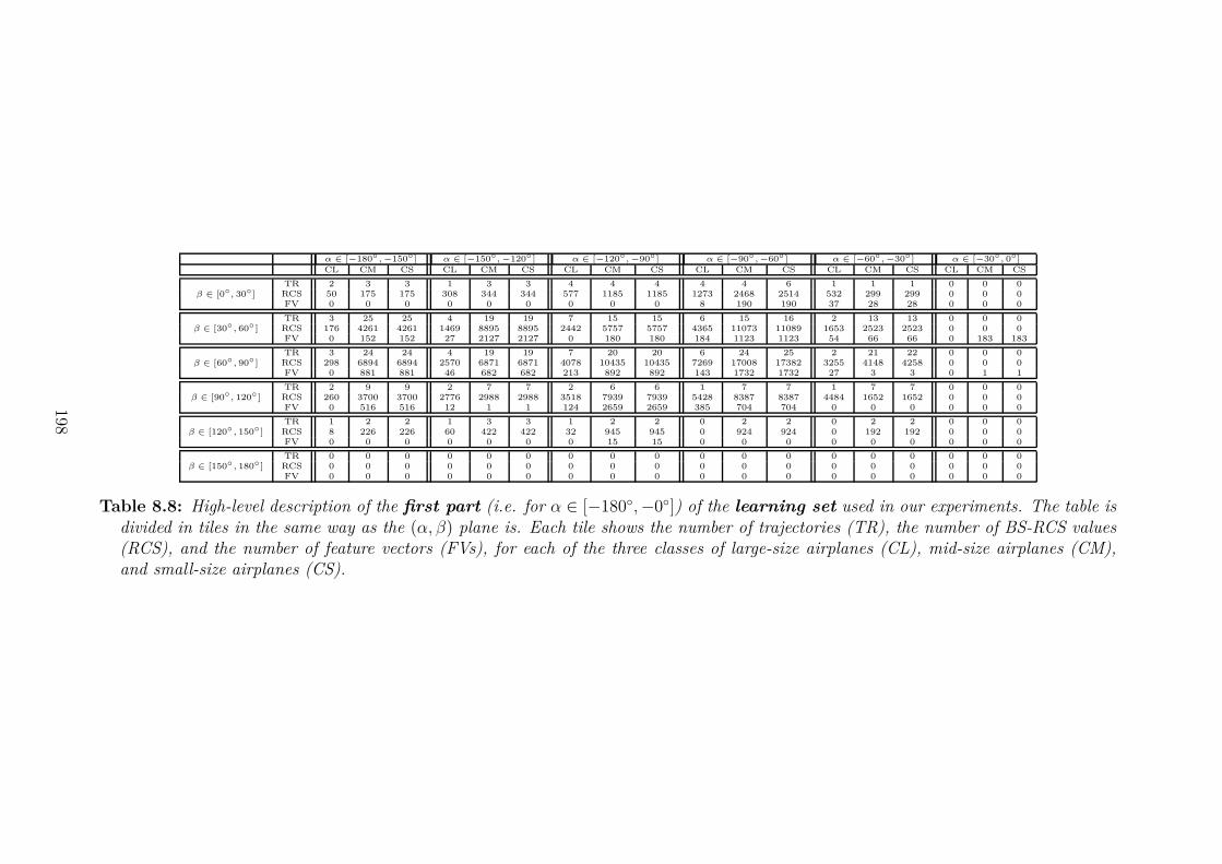
α ∈ [−180◦, −150◦ ] α ∈ [−150◦, −120◦ ] α ∈ [−120◦, −90◦] α ∈ [−90◦, −60◦ ] α ∈ [−60◦, −30◦ ] α ∈ [−30◦, 0◦]CL CM CS CL CM CS CL CM CS CL CM CS CL CM CS CL CM CS

β ∈ [0◦, 30◦]TR 2 3 3 1 3 3 4 4 4 4 4 6 1 1 1 0 0 0

RCS 50 175 175 308 344 344 577 1185 1185 1273 2468 2514 532 299 299 0 0 0FV 0 0 0 0 0 0 0 0 0 8 190 190 37 28 28 0 0 0

β ∈ [30◦, 60◦ ]TR 3 25 25 4 19 19 7 15 15 6 15 16 2 13 13 0 0 0

RCS 176 4261 4261 1469 8895 8895 2442 5757 5757 4365 11073 11089 1653 2523 2523 0 0 0FV 0 152 152 27 2127 2127 0 180 180 184 1123 1123 54 66 66 0 183 183

β ∈ [60◦, 90◦ ]TR 3 24 24 4 19 19 7 20 20 6 24 25 2 21 22 0 0 0

RCS 298 6894 6894 2570 6871 6871 4078 10435 10435 7269 17008 17382 3255 4148 4258 0 0 0FV 0 881 881 46 682 682 213 892 892 143 1732 1732 27 3 3 0 1 1

β ∈ [90◦, 120◦ ]TR 2 9 9 2 7 7 2 6 6 1 7 7 1 7 7 0 0 0

RCS 260 3700 3700 2776 2988 2988 3518 7939 7939 5428 8387 8387 4484 1652 1652 0 0 0FV 0 516 516 12 1 1 124 2659 2659 385 704 704 0 0 0 0 0 0

β ∈ [120◦, 150◦ ]TR 1 2 2 1 3 3 1 2 2 0 2 2 0 2 2 0 0 0

RCS 8 226 226 60 422 422 32 945 945 0 924 924 0 192 192 0 0 0FV 0 0 0 0 0 0 0 15 15 0 0 0 0 0 0 0 0 0

β ∈ [150◦, 180◦ ]TR 0 0 0 0 0 0 0 0 0 0 0 0 0 0 0 0 0 0

RCS 0 0 0 0 0 0 0 0 0 0 0 0 0 0 0 0 0 0FV 0 0 0 0 0 0 0 0 0 0 0 0 0 0 0 0 0 0

Table 8.8: High-level description of the first part (i.e. for α ∈ [−180◦,−0◦]) of the learning set used in our experiments. The table isdivided in tiles in the same way as the (α, β) plane is. Each tile shows the number of trajectories (TR), the number of BS-RCS values(RCS), and the number of feature vectors (FVs), for each of the three classes of large-size airplanes (CL), mid-size airplanes (CM),and small-size airplanes (CS).

198

α ∈ [0◦, 30◦ ] α ∈ [30◦, 60◦] α ∈ [60◦, 90◦ ] α ∈ [90◦, 120◦ ] α ∈ [120◦, 150◦ ] α ∈ [150◦, 180◦ ]CL CM CS CL CM CS CL CM CS CL CM CS CL CM CS CL CM CS

β ∈ [0◦, 30◦ ]TR 1 1 1 1 4 4 2 6 17 8 5 18 7 13 13 3 7 7

RCS 28 98 98 60 2015 2015 3028 3167 6313 1876 119 2560 2431 1818 1818 1864 858 858FV 0 0 0 0 189 189 1228 332 332 12 0 0 207 1 1 15 45 45

β ∈ [30◦, 60◦]TR 2 16 16 1 27 32 3 29 46 8 36 49 8 89 89 3 87 87

RCS 987 4246 4246 636 23114 24267 1806 18368 23049 4069 4231 9893 5721 31042 31042 6483 42097 42097FV 70 320 320 0 3706 3706 0 2017 2017 559 431 431 32 371 371 2098 8359 8359

β ∈ [60◦, 90◦]TR 2 15 15 1 17 17 3 21 22 6 38 39 6 86 86 3 83 83

RCS 867 7441 7441 492 22731 22731 1512 17899 17995 3859 4056 4136 7369 39773 39773 10757 55172 55172FV 0 28 28 33 4868 4868 559 4272 4272 254 1 1 564 6896 6896 526 3539 3539

β ∈ [90◦, 120◦ ]TR 1 4 4 0 4 4 1 6 6 1 12 12 1 29 29 1 28 28

RCS 236 625 625 0 2931 2931 236 1664 1664 590 748 748 6018 49419 49419 6490 81878 81878FV 0 0 0 0 1184 1184 0 0 0 0 0 0 1065 12088 12088 198 10679 10679

β ∈ [120◦, 150◦ ]TR 0 0 0 0 0 0 0 1 1 0 3 3 0 4 4 0 4 4

RCS 0 0 0 0 0 0 0 24 24 0 375 375 0 6474 6474 0 5383 5383FV 00 0 0 0 0 0 0 0 0 0 0 0 0 2141 2141 0 155 155

β ∈ [150◦, 180◦ ]TR 0 0 0 0 0 0 0 0 0 0 0 0 0 0 0 0 0 0

RCS 0 0 0 0 0 0 0 0 0 0 0 0 0 0 0 0 0 0FV 0 0 0 0 0 0 0 0 0 0 0 0 0 2158 2158 0 0 0

Table 8.9: High-level description of the second part (i.e. for α ∈ [0◦, 180◦]) of the learning set used in our experiments. See Table8.8 for additional comments.

199

α ∈ [−180◦, −150◦ ] α ∈ [−150◦, −120◦ ] α ∈ [−120◦, −90◦ ] α ∈ [−90◦, −60◦] α ∈ [−60◦, −30◦ ] α ∈ [−30◦, 0◦ ]CL CM CS CL CM CS CL CM CS CL CM CS CL CM CS CL CM CS

β ∈ [0◦, 30◦ ]TR 0 5 5 0 4 5 0 4 4 0 3 3 0 2 2 0 0 0

RCS 0 146 146 0 127 130 0 471 471 0 1460 1460 0 186 186 0 0 0FV 0 0 0 0 0 0 0 0 0 8 190 190 37 28 28 0 0 0

β ∈ [30◦, 60◦ ]TR 0 38 39 4 36 37 4 35 35 5 31 31 2 27 27 0 0 0

RCS 0 3721 3769 1452 4233 4247 2017 13181 13181 1487 13713 13713 92 5123 5123 0 0 0FV 0 152 152 46 2127 2127 0 180 180 184 1123 1123 54 66 66 0 183 183

β ∈ [60◦, 90◦ ]TR 0 37 37 5 33 33 6 42 42 6 42 42 2 38 38 0 0 0

RCS 0 8633 8633 3631 4754 4754 5219 21119 21119 2796 23332 23332 150 7254 7254 0 0 0FV 0 881 881 46 682 682 242 892 892 171 1732 1732 27 3 3 0 1 1

β ∈ [90◦, 120◦ ]TR 0 14 14 3 17 17 3 19 19 2 18 18 1 16 16 0 0 0

RCS 0 7474 7474 3000 4693 4693 4184 31422 31422 1637 28020 28020 41 9757 9757 0 0 0FV 0 516 516 12 1 1 124 2659 2659 385 704 704 0 0 0 0 0 0

β ∈ [120◦, 150◦ ]TR 0 2 2 3 12 12 3 13 13 2 12 12 1 12 12 0 0 0

RCS 0 151 151 3855 1995 1995 5082 12456 12456 2030 10500 10500 48 3699 3699 0 0 0FV 0 0 0 0 0 0 0 15 15 0 0 0 0 0 0 0 0 0

β ∈ [150◦, 180◦ ]TR 0 0 0 0 0 0 0 0 0 0 0 0 0 0 0 0 0 0

RCS 0 0 0 0 0 0 0 0 0 0 0 0 0 0 0 0 0 0FV 0 0 0 0 0 0 0 0 0 0 0 0 0 0 0 0 0 0

Table 8.10: High-level description of the first part (i.e. for α ∈ [−180◦, 0◦]) of the test set used in our experiments. See Table 8.8 foradditional comments.

200

α ∈ [0◦, 30◦ ] α ∈ [30◦, 60◦ ] α ∈ [60◦, 90◦ ] α ∈ [90◦, 120◦ ] α ∈ [120◦, 150◦ ] α ∈ [150◦, 180◦ ]CL CM CS CL CM CS CL CM CS CL CM CS CL CM CS CL CM CS

β ∈ [0◦, 30◦ ]TR 3 2 2 5 12 12 5 13 39 13 6 32 10 38 39 3 17 17

RCS 318 100 100 4122 1928 1928 8772 3819 11393 8186 62 4926 2645 4326 4371 45 1019 1019FV 0 0 0 0 189 189 1228 564 564 12 0 0 207 1 1 15 45 45

β ∈ [30◦, 60◦]TR 3 30 30 5 55 60 7 62 89 16 69 89 15 191 195 6 178 179

RCS 2243 6005 6005 4888 49296 50589 7651 40712 47973 6691 10189 20595 6578 58002 58305 1787 71019 71103FV 70 320 320 0 3588 3588 0 2017 2017 559 431 431 32 371 371 2199 8636 8636

β ∈ [60◦, 90◦]TR 3 28 28 4 34 34 4 45 48 6 67 70 7 162 162 4 169 169

RCS 2107 16020 16020 2877 44889 44889 5364 39856 39898 3046 9826 9956 1881 77973 77973 2179 105930 105930FV 0 28 28 33 4868 4868 559 4272 4272 254 1 1 565 7100 7100 526 3539 3539

β ∈ [90◦, 120◦ ]TR 0 2 2 0 4 4 0 8 8 0 17 17 1 63 63 1 68 68

RCS 0 408 408 0 1245 1245 0 1245 1245 0 5319 5319 1794 107743 107743 5175 185494 185494FV 0 0 0 0 1184 1184 0 0 0 0 0 0 1065 12088 12088 198 10679 10679

β ∈ [120◦, 150◦ ]TR 0 0 0 0 2 2 0 2 2 0 4 4 0 9 9 0 9 9

RCS 0 0 0 0 50 50 0 440 440 0 6606 6606 0 17224 17224 0 13959 13959FV 0 0 0 0 0 0 0 0 0 0 0 0 0 2141 2141 0 155 155

β ∈ [150◦, 180◦ ]TR 0 0 0 0 0 0 0 0 0 0 0 0 0 0 0 0 0 0

RCS 0 0 0 0 0 0 0 0 0 0 0 0 0 0 0 0 0 0FV 0 0 0 0 0 0 0 0 0 0 0 0 0 2158 2158 0 0 0

Table 8.11: High-level description of the second part (i.e. for α ∈ [0◦, 180◦]) of the test set used in our experiments. See Table 8.8for additional comments.

201

202 8.11. RECOGNITION EXPERIMENTS PERFORMED

8.11.2 Statistics of the feature vectors and brief analysisthereof

For each tile, we can compute the mean and standard deviation of each of the Ncomponents of all FVs built for this tile, for one class, and for one set (either the LSor the TS). Figure 8.22 shows, for one tile, for each of the three classes, and for theTS, the N values of the mean of the components of the corresponding FVs. Similarly,the figure shows the standard deviation of these components.

One can view the graph as showing representations of the mean vector and standarddeviation vector. Note that this last vector corresponds to the values along the diagonalof the covariance matrix of the FVs of interest.

1 2 3 4 5 6 7 8 9 100

0.05

0.1

0.15

0.2

0.25

0.3

0.35Mean and standard deviation vectors for TS, and for bisector sector 4 and bistatic sector 2

Index of feature vector

RC

S v

alue

[dB

]

Class 1 TS MeanClass 1 TS Std DevClass 2 TS MeanClass 2 TS Std DevClass 3 TS MeanClass 3 TS Std Dev

Figure 8.22: The figure shows the representation of the mean vector and the standarddeviation vector (diagonal of covariance matrix) of all FVs corresponding to the tiledefined by α ∈ [90◦; 120◦] and β ∈ [30◦; 60◦] and to the TS.

In Fig. 8.22, the mean vectors and the standard deviation vectors are about thesame for classes 1 and 2. Therefore, the probability of correct recognition is expectedto be low for the tile considered in the figure, as seen in Table 8.12.

In Fig. 8.23, the mean vectors and the standard deviation vectors are different forall three classes. Therefore, the probability of correct recognition is expected to behigh for the tile considered in the figure, as seen in Table 8.12.

8.11.3 Recognition results for the three-class experiment

We present in details the probabilities of correct recognition for the recognitionexperiments involving the three classes of targets. Tables 8.12, 8.13, 8.14, and 8.15give the probabilities of correct recognition for each of the four metrics defined inSection 7.5. We give in Appendix A the confusion matrices obtained for each metricand for each tile.

8.11. RECOGNITION EXPERIMENTS PERFORMED 203

1 2 3 4 5 6 7 8 9 100

0.05

0.1

0.15

0.2

0.25

0.3

0.35

0.4Mean and standard deviation vectors for TS, and for bisector sector 10 and bistatic sector 2

Index of feature vector

RC

S v

alue

[dB

]

Class 1 TS MeanClass 1 TS Std DevClass 2 TS MeanClass 2 TS Std DevClass 3 TS MeanClass 3 TS Std Dev

Figure 8.23: The figure shows the representation of the mean vector and the standarddeviation vector (diagonal of covariance matrix) of all FVs corresponding to the tiledefined by α ∈ [−120◦; −90◦] and β ∈ [30◦; 60◦] and to the TS.

For all metrics, the probability of correct recognition varies from tile to tile. Formetric E0, it ranges from 0.39 to 1. The overall probability of correct recognition,i.e. the probability of correct recognition achieved over all tiles, is of about 0.66,which is quite low. For metric E1, the probability of correct recognition variesfrom 0.35 to 0.99. The overall classification rate is of about 0.79, which is betterthan the overall classification rate achieved for the metric E0. For metric E0.05, theprobability of correct recognition varies from 0.49 to 1. The overall probability ofcorrect recognition is of about 0.83, which is better than the overall probability ofcorrect recognition achieved for metrics E0 and E1. For the aggregation of the threemetrics, the probability of correct recognition varies from 0.49 to 0.99. The overallprobability of correct recognition is of about 0.82. Therefore, it seems that metricE0.05 is to be preferred over the other metrics.

For all metrics, there are tiles for which the recognition is almost perfect. A highprobability of correct recognition is reached for α ≤ 0◦, for a constant β. No conclusioncan be drawn concerning suitable values of β, since the values of the BS-RCS areavailable for values of β ranging from 30◦ to 120◦. According to the high variationof probability of correct recognition from one tile to the other, a high probability ofcorrect recognition can be achieved by suitably locating the receiver(s) of the passivebistatic radar.

α ∈

[−180◦, −150◦ ]α ∈

[−150◦, −120◦ ]α ∈

[−120◦, −90◦ ]α ∈

[−90◦, −60◦]α ∈

[−60◦, −30◦]α ∈

[−30◦, 0◦]α ∈ [0◦, 30◦ ] α ∈ [30◦, 60◦ ] α ∈ [60◦, 90◦ ] α ∈

[90◦, 120◦ ]α ∈

[120◦, 150◦ ]α ∈

[150◦, 180◦ ]

β ∈ [0◦, 30◦] - - - 0.55 - - - 0.65 0.47 - - -β ∈ [30◦, 60◦ ] 1.0 0.76 0.99 0.52 0.92 0.88 0.66 0.58 0.61 0.66 0.63 0.51β ∈ [60◦, 90◦ ] 0.5 0.77 0.61 0.54 - - - 0.62 0.52 - 0.56 0.39β ∈

[90◦, 120◦ ]0.82 - 0.77 0.54 - - - 0.9 - - 0.4 0.5

β ∈

[120◦, 150◦ ]- - - - - - - - - - 0.62 0.9

β ∈

[150◦, 180◦ ]- - - - - - - - - - 0.75 -

Table 8.12: Weighted probabilities of correct recognition for metric E0, shown tile-by-tile, in a way similar to that of Table 8.8.

204

α ∈

[−180◦, −150◦ ]α ∈

[−150◦, −120◦ ]α ∈

[−120◦, −90◦ ]α ∈

[−90◦, −60◦]α ∈

[−60◦, −30◦]α ∈

[−30◦, 0◦]α ∈ [0◦, 30◦ ] α ∈ [30◦, 60◦] α ∈ [60◦, 90◦ ] α ∈

[90◦, 120◦ ]α ∈

[120◦, 150◦ ]α ∈

[150◦, 180◦ ]

β ∈ [0◦, 30◦] - - - 0.92 - - - 0.7 0.72 - - -β ∈ [30◦, 60◦ ] 0.93 0.85 0.88 0.86 0.88 0.93 0.74 0.77 0.89 0.84 0.82 0.77β ∈ [60◦, 90◦ ] 0.93 0.78 0.77 0.72 - - - 0.71 0.69 - 0.77 0.5β ∈

[90◦, 120◦ ]0.89 - 0.87 0.71 - - - 0.89 - - 0.72 0.35

β ∈

[120◦, 150◦ ]- - - - - - - - - - 0.77 0.99

β ∈

[150◦, 180◦ ]- - - - - - - - - - 0.8 -

Table 8.13: Weighted probabilities of correct recognition for metric E1, shown tile-by-tile, in a way similar to that of Table 8.8.

205

α ∈

[−180◦, −150◦ ]α ∈

[−150◦, −120◦ ]α ∈

[−120◦, −90◦ ]α ∈

[−90◦, −60◦]α ∈

[−60◦, −30◦]α ∈

[−30◦, 0◦]α ∈ [0◦, 30◦ ] α ∈ [30◦, 60◦ ] α ∈ [60◦, 90◦ ] α ∈

[90◦, 120◦ ]α ∈

[120◦, 150◦ ]α ∈

[150◦, 180◦ ]

β ∈ [0◦, 30◦] - - - 1.0 - - - 0.6 0.76 - - -β ∈ [30◦, 60◦ ] 0.98 0.98 1.0 0.84 0.99 0.99 0.92 0.68 0.82 0.76 0.99 0.78β ∈ [60◦, 90◦ ] 0.87 0.94 0.69 0.79 - - - 0.86 0.78 - 0.85 0.49β ∈

[90◦, 120◦ ]0.94 - 0.91 0.72 - - - 0.98 - - 0.73 0.5

β ∈

[120◦, 150◦ ]- - - - - - - - - - 0.77 1.0

β ∈

[150◦, 180◦ ]- - - - - - - - - - 0.86 -

Table 8.14: Weighted probabilities of correct recognition for metric E0.05, shown tile-by-tile, in a way similar to that of Table 8.8.

206

α ∈

[−180◦, −150◦ ]α ∈

[−150◦, −120◦ ]α ∈

[−120◦, −90◦ ]α ∈

[−90◦, −60◦]α ∈

[−60◦, −30◦]α ∈

[−30◦, 0◦]α ∈ [0◦, 30◦ ] α ∈ [30◦, 60◦] α ∈ [60◦, 90◦ ] α ∈

[90◦, 120◦ ]α ∈

[120◦, 150◦ ]α ∈

[150◦, 180◦ ]

β ∈ [0◦, 30◦] - - - 0.99 - - - 0.7 0.76 - - -β ∈ [30◦, 60◦ ] 0.98 0.91 0.96 0.88 0.99 0.96 0.88 0.78 0.91 0.85 0.93 0.79β ∈ [60◦, 90◦ ] 0.93 0.87 0.79 0.74 - - - 0.81 0.74 - 0.8 0.5β ∈

[90◦, 120◦ ]0.91 - 0.88 0.72 - - - 0.93 - - 0.73 0.49

β ∈

[120◦, 150◦ ]- - - - - - - - - - 0.77 0.99

β ∈

[150◦, 180◦ ]- - - - - - - - - - 0.83 -

Table 8.15: Weighted probabilities of correct recognition for the aggregation of the three metrics, shown tile-by-tile, in a waysimilar to that of Table 8.8.

207

208 8.12. CONCLUSION

8.11.4 Recognition results for all four recognition experiments

In order to give a general overview of the performance of the recognition system, weshow in Table 8.16 the overall probability of correct recognition for each metric andfor each of the four experiments. As can be expected from the recognition experimentinvolving the three classes of targets described above, the best probability of correctrecognition is always obtained by the E0.05 metric, for each experiment. For thethree-class experiment, the overall correct recognition rate is of 0.82. The recognitionrate is a few percent higher for the three other experiments.

Metric used Recognition experimentCL vs. CS CM vs. CS CL vs. CM CL vs. CM vs. CS

E0 0.78 0.74 0.76 0.66E1 0.77 0.87 0.76 0.79E0.05 0.87 0.88 0.83 0.84

Aggregation 0.86 0.88 0.83 0.82

Table 8.16: Overall probability of correct recognition for each of the four metrics andfor each of the four recognition experiments performed.

The probabilities of correct recognition are of the same order as the probabilitiesof correct recognition achieved for the recognition of the airplanes from their bistaticcomplex radar cross-sections, when considering a single (Tx,Rx) pair in an anechoicchamber. But, the comparison with the results achieved on data acquired in the ane-choic chamber is not pursued further as the airplanes, the frequencies, and the coveringof the (α, β) plane are different. We simply draw the conclusion that the recognizer pro-posed in Chapter 7 has been successfully tested on data acquired both in an anechoicchamber and in real outdoor conditions.

8.12 Conclusion

In this chapter, we performed the recognition of air targets by using their bistaticradar cross-sections (BS-RCSs) that we extracted from real-life signals. We presentedthe operational passive radar testdbed that we used for the acquisition of thesereal-life signals. We deployed the testbed in the vicinity of Orly Airport, using a VORas transmitter of opportunity and a software-defined radio (SDR) as receiver. Wecollected signals from a total of 1329 trajectories for 32 types of airplanes.

We performed the detection of airplanes by using the ADS-B signals they transmitfollowing interrogation. We computed the Doppler shift, the aspect angle α, thebistatic angle β, and the scene geometry from the position information present in thetransmitted ADS-B signals. We discriminated between an airplane of interest andother targets by using a Doppler filter.

We then discussed the grouping of the different detected airplanes into classes. Wedefined three classes that are the large-size airplanes, the mid-size airplanes, and the

8.12. CONCLUSION 209

small-size airplanes. For both the large-size and the mid-size airplanes, we presentedthe computation of their BS-RCS. Since small-size airplanes could not be detected byour testbed, we presented the generation of their BS-RCS from a simple model.

We also presented the data we collected, and we showed examples of receivedsignals, including spectrograms, signal-to-noise ratios, and distributions of the BS-RCSof each class of airplanes in the (α, β) plane.

We discussed the error on the position of an airplane, and showed that it hasa limited influence on the value of the BS-RCS. We also expressed the reasons forusing the BS-RCS of the airplanes instead of their bistatic complex radar cross-section(BS-CRCS).

We used the recognizer described in Chapter 7. A significant feature of thisrecognizer is that it breaks the overall recognition problem down into a set ofrecognition sub-problems by decomposing the central part of the (α, β) parameterplane into regions. We partitioned the central part of the parameter plane into acovering of 12 × 6 rectangular regions. For each region, we built one recognizer, andthus one target class model that consists in a list of subspaces that are computed fromthe feature vectors (FVs) of the airplanes. Each FV is a vector of values of BS-RCS.

We performed four recognition experiments involving the three classes of airplanes.Recognition experiment consisting in classifying air vehicles of two broad classes(large-size airplanes such as A343’s, and/or mid-size airplanes such as A319’s, and/orsmall-size airplanes such as private airplanes and UAVs), led to an overall probabilityof correct recognition varying between 0.82 and 0.88. The recognition experimentconsisting in classifying air vehicles of the three broad classes, led to an overallprobability of correct recognition of about 0.82. However, the probability of correctrecognition varies strongly according to the tile, i.e. according to the region ofthe parameter space, in which the recognition experiment is performed, rangingfrom 0.49 to 0.99. Therefore, in an operational system, one should choose the loca-tion of the receiver(s) appropriately to achieve a high probability of correct recognition.

This overall probability of correct recognition of 0.82 achieved when recognizingthe three broad classes of targets is lower than the probability of correct recognitionachieved when recognizing targets based on their radar images (Chapter 6), since fea-ture vectors contain less information than images. The overall probability of correctrecognition is however of the same order as the overall probability of correct recognitionachieved when recognizing targets based on their BS-CRCS, for a single (Tx,Rx) pair(Chapter 7). This demonstrates the potential of the recognition strategy defined inChapters 7 and 8.

210 8.12. CONCLUSION

Chapter 9

Conclusions and perspectives

Contents9.1 Conclusions . . . . . . . . . . . . . . . . . . . . . . . . . . . . 211

9.1.1 Summary of the thesis . . . . . . . . . . . . . . . . . . . . . . 211

9.1.2 Comparison of the performances of the three ATR systems . 213

9.2 Perspectives . . . . . . . . . . . . . . . . . . . . . . . . . . . . 214

9.2.1 Addition of different types of targets . . . . . . . . . . . . . . 215

9.2.2 Study of bistatic radar phenomenology . . . . . . . . . . . . . 215

9.2.3 Use of different illuminators of opportunity . . . . . . . . . . 215

9.2.4 Refinement of the recognizer . . . . . . . . . . . . . . . . . . 216

9.1 Conclusions

9.1.1 Summary of the thesis

In this thesis, we discuss the recognition of non-cooperative air targets based onpassive bistatic radar signals, i.e. on signals transmitted by one or more illuminatorsof opportunity (operating at low frequency) and scattered by an air target. The useof passive bistatic radar signals for recognition purposes is a key feature of this thesis.We indeed explained that passive bistatic radars are usually used for detection andlocation purposes. Since illuminators of opportunity are already present, the cost ofthe passive radar system is put on the receiver(s).

We focus on the recognition process. We thus assume that the targets of interestare detected and tracked, and that we know their position. We also know thelocations, the operating frequency, and the polarization of the transmitter(s) (Tx) andthe receiver(s) (Rx). We thus know the parameters of the scene.

We implement three automatic target recognition (ATR) systems. For the firstATR system, we perform the recognition of air targets by using their radar images,since many ATR systems reported in the literature use radar images for the recognitionof targets. (We explained some reasons for not recognizing targets by using theirhigh-resolution range profiles in the case of passive bistatic radar.) A radar image

211

212 9.1. CONCLUSIONS

of a target is defined as the spatial representation of the bistatic complex radarcross-section (BS-CRCS) of this target. We construct the radar images of the targetsby applying a two-dimensional (2D) inverse Fourier Transform to a 2D array of valuesof BS-CRCS of these targets.

However, we explain that the 2D diversity needed to compute 2D arrays ofvalues of BS-CRCS would hardly be met in an operational system. For thesecond ATR system, we thus perform the recognition of the air targets by directlyusing either the BS-CRCS or the bistatic radar cross-section (BS-RCS) of these targets.

Since the second ATR system is successfully tested on BS-CRCS values and BS-RCSvalues computed from signals that are acquired in an anechoic chamber, we test thisATR system on BS-RCS values that we compute from real-life signals acquired using apassive radar testbed that we deploy around Orly airport, France. We use the ADS-Bsignals transmitted by commercial airplanes to detect and locate these airplanes. Weuse a VOR Tx as illuminator of opportunity, and a software-defined radio (SDR) as Rx.

Each of the three ATR systems relies on either the BS-CRCS or the BS-RCS of thetargets of interest. We thus present the parameters the BS-CRCS and the BS-RCS arefunctions of, which are the nature of the target, the polarization of both the Tx andthe Rx, the frequency of the transmitted signal, the aspect angle of the target, andthe bistatic angle between the Tx and the Rx. In particular, the variations of boththe BS-CRCS and the BS-RCS as a function of frequency allows one to define threescattering regions. For each scattering region, the scattering mechanisms are functionof either the shape of the target, its volume, or a combination of both.

The frequency f , the polarization couple Pol, the aspect angle α, and the bistaticangle β make up the parameter space in terms of which we express both the BS-CRCSand the BS-RCS. We use this parameter space for the design of the recognition stageof each of the three ATR systems. For each recognizer, we cover the parameter spacewith tiles (overlapping or not). For each tile, we build one recognizer. The coveringof the parameter space into tiles is a key feature of the recognizer of each of the threeATR systems, and thus of this thesis.

We build each recognizer in the following way. From the input data, weproduce feature vectors (FVs). From the FVs, we construct a target class model.The class of an unknown target is determined by passing its FV through the recognizer.

For the first ATR system, an FV consists in pixel values of an ensemble of windowsextracted out of each image. The target class model consists in an ensemble ofextremely randomized trees (extra-trees). The class of an unknown target is deter-mined by propagating each window extracted from the image of this target througheach of the extra-trees. The use of tree-based methods and, thus, of extra-trees, forrecognition purposes in the radar domain is, to our knowledge, novel. Prior to ourapplication to radar images, this classification/recognition method has been used byothers on non-radar images.

For the second and third ATR systems, an FV consists in a vector of values of

9.1. CONCLUSIONS 213

either BS-CRCS or BS-RCS. The target class model consists in an ensemble of sub-spaces, each subspace characterizing a target class. The class of an unknown target isdetermined by projecting the FV of this target onto each of the subspaces of the targetclass model. We use four projection metrics to assign a class to the FV. The use ofsubspace methods for recognition purposes in the radar domain is, to our knowledge,novel.

9.1.2 Comparison of the performances of the three ATR sys-tems

We express the performances of the different ATR systems in terms of theirprobability of correct recognition, and in terms of the number of Tx’s and Rx’s used.In this section, we compare the performances of each of the three ATR systems.

We first test the first ATR system on different configurations of the well-knownMSTAR data, consisting of SAR images of ground-vehicle targets, non-targets, andSLICY targets. The highest achieved probabilities of correct recognition vary between0.96 and 0.99, depending on the configuration of the MSTAR data (targets of interestonly, targets of interest and non-targets, targets of interest and SLICY targets, ortargets of interest and SLICY and non-targets). The recognizer also proves to be quasiinsensitive to the rotation of targets.

We then test the first ATR system is on the images constructed from the ONERAdata. The images are constructed for four frequency bands, for a single polarization,for three aspect angles, and for a range of bistatic angles. We separated the rangeof bistatic angles into overlapping bistatic angular sectors. The probabilities ofcorrect recognition are very low for the lowest frequency band, and are almost perfectfor the three highest frequency bands, this for any bistatic angular sector. Thelow probabilities of correct recognition achieved at the lowest frequency band isexplained by the fact that, at theses frequencies, the BS-RCS of targets, and thusthe images, are more influenced by the volume of the targets than by their shape,the four targets having the same characteristic dimension, but different shapes.The high probabilities of correct recognition achieved at the higher frequencies areexplained by the fact that, at these frequencies, the BS-RCS of targets, and thusthe images, are more influenced by the shapes of the targets than by their volume.Even though the probabilities of correct recognition are very high, we need a highnumber of Tx’s and Rx’s in order to be able to construct the radar images of the targets.

We test the second ATR system on the ONERA data. We first recognize targets byusing their BS-CRCSs extracted for a single (Tx,Rx) pair. For the same reason as forthe images, the probabilities of correct recognition achieved for the lowest frequencyband are low, this for any polarization, any aspect angle, and any bistatic angularsector. Exactly for the same reason as for the images, the probabilities of correctrecognition increase with frequency. The probabilities of correct recognition also varyaccording to the tile of the parameter space, i.e. according to the polarization, the as-pect angle, and the bistatic angular sector. The best probabilities of correct recognitionvary from 0.33 for the lowest frequency band, up to 0.93 for the highest frequency band.

214 9.2. PERSPECTIVES

We then recognize targets by using their BS-RCSs, for a single (Tx,Rx) pair. Thebest probabilities of correct recognition vary from 0.29 for the lowest frequency band,up to 0.74 for the highest frequency band. The conclusions are exactly the same as forthe BS-RCSs. However, one must notice that the probabilities of correct recognitionachieved for the BS-CRCSs are higher than for the BS-RCSs. Therefore, the phase ofthe BS-CRCS is important, since the targets of interest have the same volume, butdifferent shapes.

The probabilities of correct recognition achieved for the recognition of targets byusing either their BS-CRCSs or their BS-RCSs extracted for a single (Tx,Rx) pair, aremuch lower than the probabilities of correct recognition achieved for the recognitionof targets by using their radar images. We thus perform the recognition of targets byusing either their BS-CRCSs or their BS-RCSs extracted for three (Tx,Rx) pairs. Theprobabilities of correct recognition increase by about 10%. Therefore, increasing thenumber of (Tx,Rx) pairs allows one to increase the probability of correct recognition.

We then test the third ATR system on real-life BS-RCSs of commercial airplanes,extracted for a single (Tx,Rx) pair. We achieve an overall probability of correctrecognition of about 0.82, with significant differences among the tiles of the (α, β)plane. We thus experimentally proved that the recognition of targets by using eithertheir BS-CRCSs or their BS-RCSs extracted from signals acquired at low frequency,in a bistatic configuration, using a limited number of (Tx,Rx) pairs gives highprobabilities of correct recognition.

According to the work presented in this thesis, an ATR system recognizing air-planes by using either their BS-CRCS or their BS-RCS, is viable, and the achievedprobabilities of correct recognition are promising. The achieved probabilities of cor-rect recognition for RCS tend to be similar to the probabilities of correct recognitionachieved for radar images, depending on the nature of the targets of interest, theiraspect angle, the bistatic angle of the configuration, the polarization of both the trans-mitter and the receiver, the frequency of the transmitted signals, and the number of(Tx,Rx) pairs used.

9.2 Perspectives

In order to completely develop and assess the performances of an ATR system usingeither the BS-RCS or the BS-RCS of targets, we need to perform further work. Wesuggest perspectives for this. These perspectives fall into four categories, discussedbelow:

• Addition of different types of targets

• Study of bistatic radar phenomenology

• Use of different illuminators of opportunity

• Refinement of the recognizer.

9.2. PERSPECTIVES 215

9.2.1 Addition of different types of targets

In this work, we considered a small number of different types of airplanes. Indeed,we tested the ATR systems on two different sets of data. The airplanes of the firstdataset were of the same size and different shapes, and the airplanes of the seconddataset were of about the same shape and different sizes. In order to validate theprinciple of recognizing air targets by using either their BS-CRCS or their BS-RCS,we should consider on a wider variety of airplanes, e.g. airplanes having both differentsizes and different shapes.

In Chapter 8, a detection stage was added to the ATR system in order to be able todetect and locate airplanes. The detection and location of airplanes, based on ADS-Bsignals, limited us to consider cooperative targets. In future work, other detection andlocation means should be envisioned, so that we can consider other targets, such assmall-size airplanes (whose BS-RCS was simulated since our testbed could not detectthem).

We could also potentially apply our ATR system to other types of targets, such asground vehicles, sea vehicles, or a mix of air, ground, and sea vehicles.

9.2.2 Study of bistatic radar phenomenology

In Chapter 3, we showed that both the BS-CRCS and the BS-RCS of targets varyaccording to the shape and size of the target, the frequency of the incident wave,the polarization of both the incident and scattered signals, the aspect angle of thetarget, and the bistatic angle between the transmitter and the receiver. In particular,we saw that the scattering mechanisms differ, for a given target, according to thefrequency band. We also experimentally showed in Chapter 6 that both the BS-CRCSand the BS-RCS of targets vary according to frequency, aspect angle, and bistatic angle.

However, a complete theoretical study of the variations of both the BS-CRCS andthe BS-RCS of different targets according to polarization, aspect angle, and bistaticangle would allow one to understand the achieved probabilities of correct recognition interms of these physical parameters. Indeed, we can simply conclude that transmittingand receiving signals at some polarization (here HH) gives higher probabilities ofcorrect recognition than at other polarizations, but we did not investigate the physicalmeaning of this observation.

Moreover, a complete phenomenological study of both the BS-CRCS and theBS-RCS would allow one to define the target classes a priori and objectively. Inthis work, targets were separated into different classes according to either their shape(Chapters 6 and 7) or their size (Chapter 8). Other ways of defining target classes canbe envisioned according, for example, to the effect of the polarization on the BS-CRCSand the BS-RCS of targets.

9.2.3 Use of different illuminators of opportunity

As we experimentally showed in Chapter 7, the probability of correct recognitionincreases when using multiple (Tx,Rx) pairs. For computational reasons, we simulated

216 9.2. PERSPECTIVES

the use of three (Tx,Rx) pairs, with a single Tx and three Rx’s. In future work, oneshould envision the use of more than three (Tx,Rx) pairs. Intuitively, the use of asmany (Tx,Rx) pairs as for the construction of the radar images should give similarprobabilities of correct recognition for both the images and the BS-CRCS (or theBS-RCS).

However, according to the work performed in Chapter 7, high probabilities ofcorrect recognition could be achieved even by using fewer (Tx,Rx) pairs than for theconstruction of radar images. Moreover, the use of more than a single Tx would allowone to perform recognition experiments over different frequency bands and differentpolarizations. The recognizer would assign a class to a given unknown target for eachfrequency band or each polarization. The final class would be given by performing amajority vote on all classes, thus resulting in a higher confidence in the recognitionresults.

The consideration of multiple (Tx,Rx) pairs would also allow one to obtain valuesof either the BS-CRCS or the BS-RCS, or both, of different targets at differentfrequencies, different polarizations, different aspect angles, and different bistaticangles, which could be used for other purposes than recognition, such as validatingthe theoretical study of bistatic phenomenology suggested above.

The VOR transmitter is the only illuminator of opportunity that we used in thisthesis, for simplicity reasons (Chapter 8). In future work, one should envision theuse of other illuminators of opportunity. The different illuminators of opportunitycould be used, simultaneously for detection, location, and recognition purposes, at lowfrequency, in a passive multistatic configuration.

In Chapter 8, we tested the ATR system on outdoor, real-life BS-RCSs. In futurework, one could process the phase of the scattered signal in order to use the BS-CRCSinstead of the BS-RCS, since we achieved higher probabilities of correct recognition forthe BS-CRCS than for the BS-RCS.

9.2.4 Refinement of the recognizer

In this thesis, we considered the recognition problem as a classification problem(in the sense of machine learning), and thus as a supervised learning problem. Weperformed the recognition of targets by using either extremely randomized treesor subspace methods. Even though we justified the use of these two recognitiontechniques in Chapters 6 and 7, one should envision investigating other classifica-tion/recognition techniques.

In this thesis, we forced the recognizer to assign a class to each unknown target,among the Nc pre-defined classes. In future work, one could envision adding the class"none" (which would stand for "none of the above"), thereby allowing the recognizer toassign to a target this additional class. This would require assigning a target class withsome degree of confidence, and to define margins between the degrees of confidence.

The partitioning of the parameter space in any number of regions offers the

9.2. PERSPECTIVES 217

possibility of running several recognizers in parallel, e.g. on a graphics processing unit(GPU), thereby enabling real-time operation.

In the different recognition experiments we performed, we defined the target classesaccording to the sizes and shapes of the different targets. The use of unsupervisedlearning techniques, such as a clustering, would allow one to experimentally define theseparation of targets into classes. Moreover, the clustering of different types of targetsshould allow one to experimentally assess the phenomenological study suggested above.

If more types of targets had been available, we could have considered classes andmeta-classes of targets, where meta-classes would be defined as groups of classes.We could have applied the Dempster-Schafer Theory of Evidence to compute theprobabilities of correct recognition of these meta-classes.

218 9.2. PERSPECTIVES

Appendices

219

Appendix A

Confusion matrices for therecognition of targets by using theirexperimentally-acquired, real-lifebistatic RCS

In Chapter 8, we perform the recognition of targets by using the bistatic radarcross-section (BS-RCS) of airplanes. The recognition experiments involve three classesof targets, which are the large-size airplanes (CL), the mid-size airplanes (CM), andthe small-size airplanes (CS). We use the recognizer we defined in Chapter 7. Foreach recognition experiment, i.e. for each tile of the parameter space, the class of anunknown target is determined by four different metrics, which are E0, E1, E0.05, andthe aggregation of the three metrics. In this appendix, we give the confusion matrixthat we obtained for each metric and for each tile of the parameter space. In eachconfusion matrix, the rows correspond to the true classes, and the columns to thecomputed classes.

Tables A.1 and A.2 show the confusion matrices achieved for each tile by usingmetric E0. Tables A.3 and A.4 show the confusion matrices achieved for each tile byusing metric E1. Tables A.5 and A.6 show the confusion matrices achieved for eachtile by using metric E0.05. Tables A.7 and A.8 show the confusion matrices achievedfor each tile for the aggregation of the three metrics.

221

α ∈ [−180◦, −150◦ ] α ∈ [−150◦, −120◦ ] α ∈ [−120◦, −90◦] α ∈ [−90◦, −60◦] α ∈ [−60◦, −30◦ ] α ∈ [−30◦, 0◦]CMc CLc CSc CMc CLc CSc CMc CLc CSc CMc CLc CSc CMc CLc CSc CMc CLc CSc

β ∈ [0◦, 30◦ ]CMt - - - - - - - - - 0.11 - - - - - - - -CLt - - - - - - - - - - - - - - - - - -CSt - - - - - - - - - 0.89 - 1.0 - - - - - -

β ∈ [30◦, 60◦ ]CMt 1.0 - - 0.54 - 0.014 1.0 - 0.011 0.25 0.13 0.12 0.97 0.24 - 0.77 - 0CLt - - - 0.008 - 0.0028 - - - 0.17 0.42 0.064 - 0.76 - - - -CSt - - 1.0 0.45 - 0.98 - - 0.99 0.58 0.45 0.81 0.03 - 1.0 0.23 - 1.0

β ∈ [60◦, 90◦ ]CMt - - - 0.55 - 0.021 0.48 0.26 0.1 0.29 0.16 0.11 - - - - - -CLt - - - - - - 0.053 0.07 0.019 0.14 0.33 0.098 - - - - - -CSt 1.0 - 1.0 0.45 - 0.98 0.47 0.67 0.88 0.57 0.5 0.8 - - - - - -

β ∈ [90◦, 120◦ ]CMt 0.7 - 0.066 - - - 0.68 0.19 0.11 0.33 0.19 0.11 - - - - - -CLt - - - - - - 0.12 0.71 0.024 0.29 0.5 0.12 - - - - - -CSt 0.3 - 0.93 - - - 0.2 0.1 0.87 0.38 0.31 0.77 - - - - - -

β ∈ [120◦, 150◦ ]CMt - - - - - - - - - - - - - - - - - -CLt - - - - - - - - - - - - - - - - - -CSt - - - - - - - - - - - - - - - - - -

β ∈ [150◦, 180◦ ]CMt - - - - - - - - - - - - - - - - - -CLt - - - - - - - - - - - - - - - - - -CSt - - - - - - - - - - - - - - - - - -

Table A.1: First set of confusion matrices (for α ∈ [−180◦, 0◦]) obtained for metric E0, shown tile-by-tile. The table is divided intiles in the same way as the (α, β) plane is. The subscripts "t" and "c" attached to CL, CM, and CS stand for "true" and "computed",respectively.

222

α ∈ [0◦, 30◦ ] α ∈ [30◦, 60◦] α ∈ [60◦, 90◦] α ∈ [90◦, 120◦ ] α ∈ [120◦, 150◦ ] α ∈ [150◦, 180◦ ]CMc CLc CSc CMc CLc CSc CMc CLc CSc CMc CLc CSc CMc CLc CSc CMc CLc CSc

β ∈ [0◦, 30◦ ]CMt - - - 0.5 - 0.21 0.1 0.027 0.013 - - - - - - - - -CLt - - - - - - 0.19 0.22 0.081 - - - - - - - - -CSt - - - 0.5 - 0.79 0.71 0.76 0.91 - - - - - - - - -

β ∈ [30◦, 60◦ ]CMt 0.62 0.34 0.19 0.39 - 0.23 0.18 - 0.068 0.2 0.068 0.029 0.28 - 0.032 0.17 0.32 0.051CLt - 0.19 - - - - - - - 0.088 0.13 0.02 - - - 0.049 0.17 0.0087CSt 0.38 0.47 0.81 0.61 - 0.77 0.82 - 0.93 0.71 0.81 0.95 0.72 - 0.97 0.78 0.51 0.94

β ∈ [60◦, 90◦ ]CMt - - - 0.48 - 0.23 0.31 0.32 0.18 - - - 0.81 0.72 0.66 0.72 0.14 0.7CLt - - - 0.005 - 0.0002 0.092 0.22 0.043 - - - 0.03 0.11 0.01 0.28 0.86 0.27CSt - - - 0.52 - 0.77 0.6 0.47 0.78 - - - 0.16 0.17 0.33 - - -

β ∈ [90◦, 120◦ ]CMt - - - 0.92 - 0.12 - - - - - - 0.43 0.31 0.36 1.0 0.81 1.0CLt - - - - - - - - - - - - 0.3 0.44 0.27 0.0008 0.19 0.0002CSt - - - 0.084 - 0.88 - - - - - - 0.27 0.26 0.37 - - -

β ∈ [120◦, 150◦ ]CMt - - - - - - - - - - - - 0.6 - 0.35 0.81 - 0.013CLt - - - - - - - - - - - - - - - - - -CSt - - - - - - - - - - - - 0.4 - 0.65 0.19 - 0.99

β ∈ [150◦, 180◦ ]CMt - - - - - - - - - - - - 0.66 - 0.15 - - -CLt - - - - - - - - - - - - - - - - - -CSt - - - - - - - - - - - - 0.34 - 0.85 - - -

Table A.2: Second set of confusion matrices (for α ∈ [0◦, 180◦]) obtained for metric E0, shown tile-by-tile. The table is divided intiles in the same way as the (α, β) plane is. The subscripts "t" and "c" attached to CL, CM, and CS stand for "true" and "computed",respectively.

223

α ∈ [−180◦, −150◦ ] α ∈ [−150◦, −120◦ ] α ∈ [−120◦, −90◦] α ∈ [−90◦, −60◦] α ∈ [−60◦, −30◦ ] α ∈ [−30◦, 0◦ ]CMc CLc CSc CMc CLc CSc CMc CLc CSc CMc CLc CSc CMc CLc CSc CMc CLc CSc

β ∈ [0◦, 30◦ ]CMt - - - - - - - - - - - - - - - - - -CLt - - - - - - - - - 1.0 - 0.16 - - - - - -CSt - - - - - - - - - - - 0.84 - - - - - -

β ∈ [30◦, 60◦ ]CMt 1.0 - 0.13 0.92 - 0.19 0.86 - - 0.8 0.16 0.041 0.83 - 0.061 1.0 - 0.016CLt - - - 0.077 - 0.041 0.14 - 0.11 0.2 0.84 0.023 0.17 1.0 0.12 - - 0.12CSt - - 0.87 - - 0.77 - - 0.89 - - 0.94 - - 0.82 - - 0.86

β ∈ [60◦, 90◦ ]CMt 0.95 - 0.095 0.87 - 0.3 0.78 0.49 0.068 0.69 0.34 0.077 - - - - - -CLt - - - 0.13 - 0.004 0.13 0.15 - 0.29 0.58 0.15 - - - - - -CSt 0.054 - 0.9 - - 0.69 0.095 0.36 0.93 0.024 0.082 0.77 - - - - - -

β ∈ [90◦, 120◦ ]CMt 1.0 - 0.21 - - - 0.92 0.1 0.049 0.63 0.3 0.077 - - - - - -CLt - - - - - - 0.075 0.9 0.13 0.37 0.65 0.11 - - - - - -CSt - - 0.79 - - - 0.001 - 0.82 0.001 0.044 0.82 - - - - - -

β ∈ [120◦, 150◦ ]CMt - - - - - - - - - - - - - - - - - -CLt - - - - - - - - - - - - - - - - - -CSt - - - - - - - - - - - - - - - - - -

β ∈ [150◦, 180◦ ]CMt - - - - - - - - - - - - - - - - - -CLt - - - - - - - - - - - - - - - - - 0CSt - - - - - - - - - - - - - - - - - -

Table A.3: First set of confusion matrices (for α ∈ [−180◦, 0◦]) obtained for metric E1, shown tile-by-tile. The table is divided intiles in the same way as the (α, β) plane is. The subscripts "t" and "c" attached to CL, CM, and CS stand for "true" and "computed",respectively.

224

α ∈ [0◦, 30◦] α ∈ [30◦, 60◦ ] α ∈ [60◦, 90◦ ] α ∈ [90◦, 120◦ ] α ∈ [120◦, 150◦ ] α ∈ [150◦, 180◦ ]CMc CLc CSc CMc CLc CSc CMc CLc CSc CMc CLc CSc CMc CLc CSc CMc CLc CSc

β ∈ [0◦, 30◦ ]CMt - - - 0.66 - 0.25 0.66 0.31 0.15 - - - - - - - - -CLt - - - - - - 0.32 0.69 0.067 - - - - - - - - -CSt - - - 0.34 - 0.75 0.016 0.004 0.78 - - - - - - - - -

β ∈ [30◦, 60◦ ]CMt 0.69 0.39 0.17 0.74 - 0.19 0.92 - 0.13 0.52 0.31 0.0006 0.8 - 0.13 0.77 0.34 0.007CLt 0.31 0.61 0.025 - - - - - - 0.38 0.59 0.001 0.2 - 0.024 0.14 0.66 0.19CSt - - 0.81 0.26 - 0.81 0.083 - 0.87 0.097 0.095 1.0 - - 0.85 0.09 - 0.81

β ∈ [60◦, 90◦ ]CMt - - - 0.74 - 0.24 0.7 0.33 0.27 - - - 0.78 0.33 0.2 0.94 0.13 0.39CLt - - - 0.19 - 0.084 0.28 0.63 0.045 - - - 0.15 0.67 0.04 0.06 0.87 0.59CSt - - - 0.065 - 0.67 0.026 0.038 0.69 - - - 0.066 - 0.76 - - -

β ∈ [90◦, 120◦ ]CMt - - - 0.98 - 0.2 - - - - - - 0.83 0.24 0.24 0.7 0.4 0.93CLt - - - - - - - - - - - - 0.093 0.33 0.1 0.3 0.6 0.065CSt - - - 0.016 - 0.8 - - - - - - 0.08 0.44 0.65 - - -

β ∈ [120◦, 150◦ ]CMt - - - - - - - - - - - - 0.87 - 0.33 1.0 - 0.026CLt - - - - - - - - - - - - - - - - - -CSt - - - - - - - - - - - - 0.13 - 0.67 - - 0.97

β ∈ [150◦, 180◦ ]CMt - - - - - - - - - - - - 0.86 - 0.27 - - -CLt - - - - - - - - - - - - - - - - - -CSt - - - - - - - - - - - - 0.14 - 0.73 - - -

Table A.4: Second set of confusion matrices (for α ∈ [0◦; 180◦]) obtained for metric E1, shown tile-by-tile. The table is divided intiles in the same way as the (α, β) plane is. The subscripts "t" and "c" attached to CL, CM, and CS stand for "true" and "computed",respectively.

225

α ∈ [−180◦, −150◦ ] α ∈ [−150◦, −120◦ ] α ∈ [−120◦, −90◦ ] α ∈ [−90◦, −60◦] α ∈ [−60◦, −30◦ ] α ∈ [−30◦, 0◦]CMc CLc CSc CMc CLc CSc CMc CLc CSc CMc CLc CSc CMc CLc CSc CMc CLc CSc

β ∈ [0◦, 30◦ ]CMt - - - - - - - - - 1.0 - - - - - - - -CLt - - - - - - - - - - - - - - - - - -CSt - - - - - - - - - - - 1.0 - - - - - -

β ∈ [30◦, 60◦]CMt 1.0 - 0.039 0.98 - 0.01 1.0 - 0.006 0.7 0.14 0.021 0.98 - - 1.0 - -CLt - - - 0.024 - 0.004 - - - 0.18 0.85 0.001 0.015 1.0 - - - 0.016CSt - - 0.96 0.0005 - 0.99 - - 0.99 0.12 0.011 0.98 - - 1.0 - - 0.98

β ∈ [60◦, 90◦]CMt 0.74 - 0.008 0.92 - 0.034 0.59 0.29 0.02 0.67 0.22 0.059 - - - - - -CLt - - - 0.004 - - 0.034 0.05 - 0.26 0.64 0.031 - - - - - -CSt 0.26 - 0.99 0.075 - 0.97 0.38 0.66 0.98 0.065 0.13 0.91 - - - - - -

β ∈ [90◦, 120◦ ]CMt 0.98 - 0.11 - - - 0.9 0.056 0.03 0.51 0.2 0.06 - - - - - -CLt - - - - - - 0.083 0.94 0.055 0.45 0.74 0.018 - - - - - -CSt 0.016 - 0.89 - - - 0.015 - 0.91 0.036 0.062 0.92 - - - - - -

β ∈ [120◦, 150◦ ]CMt - - - - - - - - - - - - - - - - - -CLt - - - - - - - - - - - - - - - - - -CSt - - - - - - - - - - - - - - - - - -

β ∈ [150◦, 180◦ ]CMt - - - - - - - - - - - - - - - - - -CLt - - - - - - - - - - - - - - - - - -CSt - - - - - - - - - - - - - - - - - -

Table A.5: First set of confusion matrices (for α ∈ [−180◦, 0◦]) obtained for metric E0.05, shown tile-by-tile. The table is divided intiles in the same way as the (α, β) plane is. The subscripts "t" and "c" attached to CL, CM, and CS stand for "true" and "computed",respectively..

226

α ∈ [0◦, 30◦ ] α ∈ [30◦, 60◦] α ∈ [60◦, 90◦] α ∈ [90◦, 120◦ ] α ∈ [120◦, 150◦ ] α ∈ [150◦, 180◦ ]CMc CLc CSc CMc CLc CSc CMc CLc CSc CMc CLc CSc CMc CLc CSc CMc CLc CSc

β ∈ [0◦, 30◦ ]CMt - - - 0.43 - 0.22 0.37 0.2 0.011 - - - - - - - - -CLt - - - - - - 0.32 0.73 0.018 - - - - - - - - -CSt - - - 0.57 - 0.78 0.31 0.068 0.97 - - - - - - - - -

β ∈ [30◦, 60◦ ]CMt 0.97 0.56 0.037 0.43 - 0.081 0.6 - 0.02 0.43 0.21 0.001 0.99 - 0.016 0.62 0.33 0.002CLt 0.025 0.44 - - - - - - - 0.13 0.31 - 0.011 - - 0.089 0.65 0.007CSt - - 0.96 0.57 - 0.92 0.4 - 0.98 0.43 0.48 1.0 - - 0.98 0.29 0.018 0.99

β ∈ [60◦, 90◦ ]CMt - - - 0.85 - 0.12 0.77 0.42 0.15 - - - 0.9 0.46 0.17 0.93 0.14 0.64CLt - - - 0.016 - 0.003 0.097 0.31 0.011 - - - 0.035 0.49 0.004 0.072 0.86 0.33CSt - - - 0.14 - 0.87 0.13 0.27 0.84 - - - 0.07 0.051 0.83 - - -

β ∈ [90◦, 120◦ ]CMt - - - 0.98 - 0.024 - - - - - - 0.8 0.17 0.24 1.0 0.69 1.0CLt - - - - - - - - - - - - 0.1 0.46 0.077 0.003 0.31 0.0005CSt - - - 0.017 - 0.98 - - - - - - 0.099 0.37 0.69 - - -

β ∈ [120◦, 150◦ ]CMt - - - - - - - - - - - - 0.85 - 0.3 1.0 - -CLt - - - - - - - - - - - - - - - - - -CSt - - - - - - - - - - - - 0.15 - 0.7 - - 1.0

β ∈ [150◦, 180◦ ]CMt - - - - - - - - - - - - 0.82 - 0.091 - - -CLt - - - - - - - - - - - - - - - - - -CSt - - - - - - - - - - - - 0.18 - 0.91 - - -

Table A.6: Second set of confusion matrices (for α ∈ [0◦; 180◦]) obtained for metric E0.05, shown tile-by-tile. The table is divided intiles in the same way as the (α, β) plane is. The subscripts "t" and "c" attached to CL, CM, and CS stand for "true" and "computed",respectively.

227

α ∈ [−180◦, −150◦ ] α ∈ [−150◦, −120◦ ] α ∈ [−120◦, −90◦ ] α ∈ [−90◦, −60◦] α ∈ [−60◦, −30◦ ] α ∈ [−30◦, 0◦ ]CMc CLc CSc CMc CLc CSc CMc CLc CSc CMc CLc CSc CMc CLc CSc CMc CLc CSc

β ∈ [0◦, 30◦]CMt - - - - - - - - - 1.0 - 0.016 - - - - - -CLt - - - - - - - - - - - - - - - - - -CSt - - - - - - - - - - - 0.98 - - - - - -

β ∈ [30◦, 60◦ ]CMt 1.0 - 0.046 0.95 - 0.12 0.92 - - 0.82 0.11 0.038 0.97 - - 1.0 - 0.006CLt - - - 0.047 - 0.016 0.083 - - 0.18 0.89 0.013 0.03 1.0 - - - 0.077CSt - - 0.95 - - 0.87 - - 1.0 0.005 - 0.95 - - 1.0 - - 0.92

β ∈ [60◦, 90◦ ]CMt 0.94 - 0.07 0.97 - 0.23 0.79 0.46 0.027 0.71 0.25 0.13 - - - - - -CLt - - - 0.028 - 0.002 0.059 0.095 - 0.27 0.66 0.097 - - - - - -CSt 0.064 - 0.93 0.003 - 0.77 0.15 0.44 0.97 0.027 0.094 0.78 - - - - - -

β ∈ [90◦, 120◦ ]CMt 1.0 - 0.18 - - - 0.92 0.081 0.052 0.63 0.25 0.089 - - - - - -CLt - - - - - - 0.079 0.92 0.11 0.37 0.7 0.082 - - - - - -CSt - - 0.82 - - - 0.001 - 0.83 0.001 0.042 0.83 - - - - - -

β ∈ [120◦, 150◦ ]CMt - - - - - - - - - - - - - - - - - -CLt - - - - - - - - - - - - - - - - - -CSt - - - - - - - - - - - - - - - - - -

β ∈ [150◦, 180◦ ]CMt - - - - - - - - - - - - - - - - - -CLt - - - - - - - - - - - - - - - - - -CSt - - - - - - - - - - - - - - - - - -

Table A.7: First set of confusion matrices (for α ∈ [−180◦; 0◦]) obtained for the aggregation of the three metrics, shown tile-by-tile. The table is divided in tiles in the same way as the (α, β) plane is. The subscripts "t" and "c" attached to CL, CM, and CS standfor "true" and "computed", respectively.

228

α ∈ [0◦, 30◦] α ∈ [30◦, 60◦] α ∈ [60◦, 90◦] α ∈ [90◦, 120◦ ] α ∈ [120◦, 150◦ ] α ∈ [150◦, 180◦ ]CMc CLc CSc CMc CLc CSc CMc CLc CSc CMc CLc CSc CMc CLc CSc CMc CLc CSc

β ∈ [0◦, 30◦ ]CMt - - - 0.64 - 0.25 0.57 0.25 0.063 - - - - - - - - -CLt - - - - - - 0.41 0.74 0.07 - - - - - - - - -CSt - - - 0.36 - 0.75 0.023 0.015 0.87 - - - - - - - - -

β ∈ [30◦, 60◦ ]CMt 0.97 0.49 0.14 0.69 - 0.14 0.87 - 0.056 0.61 0.31 0.001 0.95 - 0.092 0.76 0.34 0.004CLt 0.028 0.51 - - - - - - - 0.26 0.57 - 0.051 - 0.003 0.13 0.66 0.13CSt - - 0.86 0.31 - 0.86 0.13 - 0.94 0.13 0.12 1.0 - - 0.91 0.11 - 0.86

β ∈ [60◦, 90◦ ]CMt - - - 0.88 - 0.25 0.76 0.36 0.25 - - - 0.84 0.35 0.22 0.94 0.12 0.55CLt - - - 0.049 - 0.015 0.2 0.61 0.024 - - - 0.079 0.65 0.017 0.059 0.88 0.45CSt - - - 0.068 - 0.74 0.037 0.036 0.73 - - - 0.077 - 0.77 - - -

β ∈ [90◦, 120◦ ]CMt - - - 0.98 - 0.12 - - - - - - 0.83 0.22 0.25 0.99 0.56 1.0CLt - - - - - - - - - - - - 0.089 0.35 0.093 0.01 0.44 0.002CSt - - - 0.017 - 0.88 - - - - - - 0.084 0.44 0.66 - - -

β ∈ [120◦, 150◦ ]CMt - - - - - - - - - - - - 0.87 - 0.32 1.0 - 0.013CLt - - - - - - - - - - - - - - - - - -CSt - - - - - - - - - - - - 0.13 - 0.68 - - 0.99

β ∈ [150◦, 180◦ ]CMt - - - - - - - - - - - - 0.86 - 0.2 - - -CLt - - - - - - - - - - - - - - - - - -CSt - - - - - - - - - - - - 0.14 - 0.8 - - -

Table A.8: Second set of confusion matrices (for α ∈ [0◦; 180◦]) obtained for the aggregation of the three metrics, showntile-by-tile. The table is divided in tiles in the same way as the (α, β) plane is. The subscripts "t" and "c" attached to CL, CM, and CSstand for "true" and "computed", respectively.

229

230

Appendix B

Publications

Different parts of this work have been published as journal articles or as conferencepapers. We list them below.

2.1 Journal articles

• J. Pisane, S. Azarian, M. Lesturgie, J. G. Verly, Automatic target recognition(ATR) for passive radar, To appear in IEEE Transactions on Aerospace andElectronic Systems.

2.2 Conference papers

• J. Pisane, S. Azarian, M. Lesturgie, J. G. Verly, Passive radar testbed and prelim-inary experiments in recognition of non-cooperative aircraft intruding into con-trolled airspace, URSI Benelux Forum, Sept. 2012 [150].

• J. Pisane, S. Azarian, M. Lesturgie, J. G. Verly, Automatic real-time collection ofRCS of airplanes in a real bistatic low-frequency configuration using a softwaredefined passive radar based on illuminators of opportunity, International RadarConference, May 2012 [149].

• J. Pisane, M. Lesturgie, J. G. Verly, Target classification system based on thecharacterization of targets by subspaces, IEEE CIE International Conference onRadar, Oct. 2011 [154].

• J. Pisane, M. Lesturgie, J. G. Verly, Passive target classification based on low-frequency bistatic backscattering coefficients, Ocean & Coastal Observation: Sen-sors and Systems, Passive Session, June 2010 [152].

• J. Pisane, R. Marée, L. Wehenkel, and J. G. Verly, Robust Automatic TargetRecognition Using Extra-trees, International Radar Conference, IEEE, May 2010[157].

• J. Pisane, M. Lesturgie, and J. G. Verly. Target classification of experimentally-acquired low-frequency backscattering coefficients by construction of subspaces,URSI Benelux Forum, April 2010 [153].

231

232 2.3. OTHER PUBLICATIONS

• J. Pisane, R. Marée, P. Ries, L. Wehenkel, and J. G. Verly, An Extra-trees-basedAutomatic Target Recognition Algorithm, International Radar Conference, IEEE,Oct. 2009 [155].

2.3 Other publications

• J. Pisane, S. Azarian, M. Lesturgie, J. G. Verly, Target classification in bistaticlow frequency radar, 2nd Thales Radar PhD Day, Sept. 2012 [151].

• J. Pisane, R. Marée, L. Wehenkel, and J. G. Verly, Radar Classification based onExtra-Trees, SONDRA Workshop, May 2010 [156].

Bibliography

[1] Abramowitz, M., and Stegun, I. Handbook of mathematical functions: withformulas, graphs, and mathematical tables. Dover publications, 1965. (page 40).

[2] Airbus. Airbus, an EADS company. Website, 2012. http://www.airbus.com/

aircraftfamilies/. (page 174).

[3] Alcatel Lucent Chair on Flexible Radio. Sdr4all. Website, 2012.http://www.flexible-radio.com/sdr4all. (page 183).

[4] Anderson, S. Target classification, recognition and identification with HFradar. In Proceedings of the NATO Research and Technology Agency. Sensorsand Electronics Technology Panel Symposium SET–080/RSY17/RFT: “Targetidentification and recognition using RF systems”, RTO–MP–SET (2004). (page18).

[5] Asano, F., Hayamizu, S., Yamada, T., and Nakamura, S. Speech en-hancement based on the subspace method. IEEE Transactions on Speech andAudio Processing (2000). (page 143).

[6] Baker, C., and Griffiths, H. Bistatic and multistatic radar sensors forhomeland security. Advances in sensing with security applications (2006). (page16).

[7] Baker, C., Griffiths, H., and Papoutsis, I. Passive coherent locationradar systems. Part 2: Waveform properties. In IEE Proceedings Radar, Sonar,and Navigation (2005). (page 16).

[8] Balanis, C. Antenna theory: analysis and design. J. Wiley, 1982. (pages 26,32).

[9] Baldwin, J., Smith, A., and Cassell, R. General aviation colli-sion avoidance-challenges of full implementation. In Proceedings of the 13thAIAA/IEEE Digital Avionics Systems Conference (DASC) (1994). (page 11).

[10] Bandiera, F., Besson, O., Orlando, D., Ricci, G., and Scharf, L.GLRT-based direction detectors in noise and subspace interference. In Proceed-ings of the IEEE International Conference on Acoustics, Speech, and Signal Pro-cessing (ICASSP) (2006). (page 143).

[11] Bandiera, F., De Maio, A., Greco, A., and Ricci, G. Adaptive radardetection of distributed targets in homogeneous and partially homogeneous noiseplus subspace interference. IEEE Transactions on Signal Processing (2007). (page143).

233

234 BIBLIOGRAPHY

[12] Bandiera, F., Orlando, D., Ricci, G., and Scharf, L. Adaptive radardetection: A subspace identification approach. In Proceedings of the 2nd In-ternational Workshop on Cognitive Information Processing (CIP) (2010). (page143).

[13] Barès, C. Développement et application de méthodes d’identification de ciblesaériennes dans les bandes HF et VHF. PhD thesis, Université de Rennes I, 2007.(page 20).

[14] Behrens, R., Scharf, L., Inc, C., and Broomfield, C. Signal process-ing applications of oblique projection operators. IEEE Transactions on SignalProcessing (1994). (pages 146, 148).

[15] Belkacemi, H. Approches de sous-espaces pour le traitement adaptatif spatio-temporel en radar aéroporté monostatique/bistatique. PhD thesis, Université deParis XI Orsay, 2006. (page 143).

[16] Bencheikh, M. L., Wang, Y., and He, H. A subspace-based technique forjoint DOA-DOD estimation in bistatic MIMO radar. In Proceedings of the 11thInternational Radar Symposium (IRS) (2010). (page 143).

[17] Bhanu, B. Automatic target recognition: State of the art survey. IEEE Trans-actions on Aerospace and Electronic Systems (1986). (pages 2, 17, 18).

[18] Blyakhman, A., and Runova, I. Forward scattering radiolocation bistaticRCS and target detection. In The Record of the 1999 IEEE Radar Conference(1999). (page 16).

[19] Boeing. Boeing, commercial airplanes. Website, 2012.http://www.boeing.com/commercial/products.html. (page 175).

[20] Boerner, W., Yan, W., Xi, A., and Yamaguchi, Y. Basic concepts ofradar polarimetry. Proceedings of the NATO Advanced Research Workshop onDirect and Inverse Methods in Radar Polarimetry (1988). (page 50).

[21] Boerner, W., Yan, W., Xi, A., and Yamaguchi, Y. On the basic princi-ples of radar polarimetry: The target characteristic polarization state theory ofKennaugh, Huynen’s polarization fork concept, and its extension to the partiallypolarized case. Proceedings of the IEEE (1991). (page 50).

[22] Boisvert, R., and Orlando, V. ADS-Mode S system overview. In Pro-ceedings of the 12th AIAA/IEEE Digital Avionics Systems Conference (DASC)(1993). (page 11).

[23] Born, M., and Wolf, E. Principles of optics: electromagnetic theory ofpropagation, interference and diffraction of light. Pergamon Press, 1965. (pages32, 35).

[24] Bracewell, R. Two-dimensional imaging. Prentice-Hall, 1995. (pages 19, 80,81, 82, 84, 87).

[25] Breiman, L. Classification and regression trees. Chapman & Hall/CRC, 1984.(page 113).

BIBLIOGRAPHY 235

[26] Breiman, L. Bagging predictors. Machine learning (1996). (page 113).

[27] Breiman, L. Random forests. Machine learning (2001). (page 113).

[28] Breiman, L., Friedman, J., Olsen, R., and Stone, C. Classification andregression trees. Wadsworth International, 1984. (page 115).

[29] Brigui, F. Algorithmes d’imagerie SAR polarimétrique basés sur des modèles àsous-espace. PhD thesis, SUPELEC, 2010. (page 143).

[30] Brousseau, C. Caractérisation Large Bande de Fréquence: Application auradar et au sondage de canal. PhD thesis, Université Rennes 1, 2005. (page 20).

[31] Cetin, M., Karl, W., and Castanon, D. Analysis of the impact of feature-enhanced SAR imaging on ATR performance. In Proceedings of SPIE (2002),vol. 4727. (page 20).

[32] Cetin, M., and Lanterman, A. Region-enhanced passive radar imaging. InIEE Proceedings Radar, Sonar, and Navigation (2005). (page 19).

[33] Cha, P., and Molinder, J. Fundamentals of signals and systems: a buildingblock approach. Cambridge Univ Press, 2006. (page 105).

[34] Challa, S., and Koks, D. Bayesian and Dempster-Shafer fusion. Sadhana(2004). (page 148).

[35] Chassay, G. Justification du modèle des points brillants. intégration dans lemodèle des interactions entre différentes parties d’une cible. In 9eme Colloquesur le traitement du signal et des images (1983), Groupe d’Etudes du Traitementdu Signal et des Images (GRETSI). (pages 145, 196).

[36] Chen, C.-Y., and Vaidyanathan, P. A Subspace Method for MIMO RadarSpace-Time Adaptive Processing. In Proceedings of the IEEE International Con-ference on Acoustics, Speech, and Signal Processing (ICASSP) (2007). (page143).

[37] Chen, J., and Walton, E. Comparison of two target classification techniques.IEEE Transactions on Aerospace and Electronic Systems (1986). (page 19).

[38] Chen, V., and Ling, H. Joint time-frequency analysis for radar signal andimage processing. IEEE Signal Processing Magazine (1999). (page 20).

[39] Cherniakov, M., Abdullah, R., Jancovic, P., and Salous, M. Forwardscattering micro sensor for vehicle classification. In Proceedings of the IEEEInternational Radar Conference (2005). (page 39).

[40] Cherniakov, M., Abdullah, R., Jancovic, P., Salous, M., and Cha-pursky, V. Automatic ground target classification using forward scatteringradar. In IEE Proceedings Radar, Sonar, and Navigation (2006). (page 39).

[41] Cherniakov, M., and Nezlin, D. Bistatic radar: principles and practice.John Wiley, 2007. (pages 27, 30, 41, 42, 92).

236 BIBLIOGRAPHY

[42] Cherniakov, M., Nezlin, D., and Kubik, K. Air target detection viabistatic radar based on LEOS communication signals. In IEE Proceedings Radar,Sonar, and Navigation (2002). (page 17).

[43] Cherniakov, M., Salous, M., Kostylev, V., and Abdullah, R. Analysisof forward scattering radar for ground target detection. In Proceedings of theIEEE European Radar Conference (EURAD) (2005). (page 39).

[44] Cohen, M. An overview of radar-based, automatic, noncooperative target recog-nition techniques. In Proceedings of the IEEE International Conference on Sys-tems Engineering (1991). (pages 17, 18).

[45] Coleman, C., Watson, R., and Yardley, H. A practical bistatic passiveradar system for use with DAB and DRM illuminators. In Proceedings of theIEEE Radar Conference (2008). (page 17).

[46] Colin-Koeniguer, E., and Thirion-Lefevre, L. Bistatic scattering fromforest components. Part II: first validation of a bistatic polarimetric forest modelin the VHF-UHF band [225–475 MHz] using indoor measurements. Waves inRandom and Complex Media (2010). (pages 26, 55).

[47] Colone, F., O’Hagan, D., Lombardo, P., and Baker, C. A multi-stage processing algorithm for disturbance removal and target detection in pas-sive bistatic radar. IEEE Transactions on Aerospace and Electronic Systems(2009). (page 16).

[48] Crispin, J., Siegel, K., and Bowman, J. Methods of radar cross-sectionanalysis. Academic Press, 1968. (pages 15, 42).

[49] Crispin Jr, J., Goodrich, R., and Siegel, K. A theoretical method for thecalculation of radar cross section of aircraft and missiles. Tech. rep., Universityof Michigan, 1959. (pages 15, 31, 32, 35, 36, 37, 40, 41).

[50] Crispin Jr, J., and Maffett, A. Radar cross-section estimation for simpleshapes. Proceedings of the IEEE (1965). (pages 31, 32).

[51] Cumming, I., and Wong, F. Digital signal processing of synthetic apertureradar data: algorithms & implementation. Artech House, 2005. (page 19).

[52] Du, L., Liu, H., and Bao, Z. Radar HRRP statistical recognition: Parametricmodel and model selection. IEEE Transactions on Signal Processing (2008).(page 19).

[53] Duda, R., and Hart, P. Pattern classification and scene analysis. Wiley,1996. (page 106).

[54] Duda, R., Hart, P., and Stork, D. Pattern classification and scene analysis2nd ed. Wiley Interscience, 1995. (pages 2, 114).

[55] Dudgeon, D., and Lacoss, R. An overview of automatic target recognition.The Lincoln Laboratory Journal (1993). (page 18).

BIBLIOGRAPHY 237

[56] Dumont, M., Marée, R., Wehenkel, L., and Geurts, P. Fast multi-class image annotation with random subwindows and multiple output randomizedtrees. In Proceedings of the International Conference on Computer Vision Theoryand Applications (VISAPP) (2009). (page 116).

[57] Duquenoy, M. Analyse temps-fréquence appliquée à l’imagerie SAR po-larimétrique. PhD thesis, Université Rennes 1, 2009. (page 145).

[58] Durand, R. Processeurs SAR basés sur des détecteurs de sous-espaces. PhDthesis, SUPELEC, 2007. (page 143).

[59] Ehrman, L. Automatic target recognition using passive radar and a coordinatedflight model. Master’s thesis, Georgia Institute of Technology, 2004. (page 21).

[60] Ehrman, L. An algorithm for automatic target recognition using passive radarand an EKF for estimating aircraft orientation. PhD thesis, Georgia Institute ofTechnology, 2005. (page 21).

[61] Ehrman, L., and Lanterman, A. Automatic target recognition via passiveradar, using precomputed radar cross sections and a coordinated flight model.IEEE Transactions on Aerospace and Electronic Systems (2003). (page 21).

[62] Ehrman, L., and Lanterman, A. Target identification using modeled radarcross sections and a coordinated flight model. In Proceedings from the ThirdMulti-National Conference on Passive and Covert Radar (2003). (page 21).

[63] Ehrman, L., and Lanterman, A. A robust algorithm for automated tar-get recognition using precomputed radar cross sections. In Proceedings of SPIE(2004), vol. 5426, Citeseer. (page 21).

[64] Ehrman, L., and Lanterman, A. A robust algorithm for automatic targetrecognition using passive radar. In System Theory, Proceedings of the Thirty-Sixth Southeastern Symposium on (2004), IEEE. (page 21).

[65] Eigel Jr, R., Collins, P., Terzuoli Jr, A., Nesti, G., and Fortuny,J. Bistatic scattering characterization of complex objects. IEEE Transactionson Geoscience and Remote Sensing (2000). (pages 28, 30, 31, 42).

[66] Eisenbies, C. Classification of ultra high range resolution radar using decisionboundary analysis. Tech. rep., DTIC Document, 1994. (page 19).

[67] Flightradar24 AB. Flightradar24, live air traffic. Website, 2012.http://www.flightradar24.com. (pages 172, 181).

[68] Florin, C. Automated traffic control for smart landing facilities. PhD thesis,Virginia Polytechnic Institute and State University, 2002. (page 10).

[69] Geurts, P., Ernst, D., and Wehenkel, L. Extremely randomized trees.Machine learning (2006). (pages 113, 115).

[70] Gini, F., Giannakis, G., Greco, M., and Zhou, G. T. Time-averagedsubspace methods for radar clutter texture retrieval. IEEE Transactions onSignal Processing (2001). (page 143).

238 BIBLIOGRAPHY

[71] Glende, M., Heckenbach, J., Kuschel, H., Müller, S., Schell, J.,and Schumacher, C. Experimental passive radar systems using digital illu-minators (DAB/DVB-T). In Proceedings of the International Radar Symposium(IRS) (2007). (page 17).

[72] Greco, M., Gini, F., and Farina, A. A multiple hypotheses testing ap-proach to radar detection and pre-classification. In Proceedings of the IEEERadar Conference (2004). (page 147).

[73] Griffiths, H. Bistatic radar - principles and practice. In Proceedings of theSBMO International Microwave Conference (1993). (page 16).

[74] Griffiths, H. From a different perspective: principles, practice and potentialof bistatic radar. In Proceedings of the International Radar Conference (2003).(page 16).

[75] Griffiths, H. New directions in bistatic radar. In Proceedings of the IEEERadar Conference (2008), IEEE. (page 16).

[76] Griffiths, H., and Baker, C. Passive coherent location radar systems. Part1: Performance prediction. In IEE Proceedings Radar, Sonar, and Navigation(2005). (page 16).

[77] Griffiths, H., and Long, N. Television-based bistatic radar. IEE ProceedingsCommunications, Radar, and Signal Processing (1986). (page 17).

[78] Griffiths, H., and Willis, N. Klein Heidelberg - The first modern bistaticradar system. IEEE Transactions on Aerospace and Electronic Systems (2010).(page 16).

[79] Gunal, S., and Edizkan, R. Use of novel feature extraction technique withsubspace classifiers for speech recognition. In Proceedings of the IEEE Interna-tional Conference on Pervasive Services (2007). (page 143).

[80] Guo, H., Coetzee, S., Mason, D., Woodbridge, K., and Baker, C.Passive radar detection using wireless networks. In Proceedings of the IET In-ternational Conference on Radar Systems (2007). (page 17).

[81] Guo, H., Woodbridge, K., and Baker, C. Evaluation of WiFi beacontransmissions for wireless based passive radar. In Proceedings of the IEEE RadarConference (2008). (page 17).

[82] Herman, S., and Moulin, P. A particle filtering approach to FM-band passiveradar tracking and automatic target recognition. In IEEE Aerospace ConferenceProceedings (2002). (page 21).

[83] Hernandez, N., Rodriguez, J., Martin, J., Mata, F., Gonzalez, R.,and Alvarez, R. An approach to automatic target recognition in radar imagesusing SVM. Lecture Notes in Computer Science (2006). (page 20).

[84] Holpp, W. The century of radar. Deutsche Gesellschaft für Ortung und Navi-gation (DGON) (2003). (page 15).

BIBLIOGRAPHY 239

[85] Howland, P. Target tracking using television-based bistatic radar. In IEEProceedings Radar, Sonar, and Navigation (1999). (page 17).

[86] Howland, P., Maksimiuk, D., and Reitsma, G. FM radio based bistaticradar. In IEE Proceedings Radar, Sonar and Navigation (2005), IET. (page 17).

[87] Huynen, J. Phenomenological theory of radar targets. PhD thesis, DrukkerijBronder-Offset NV, 1970. (pages 52, 53).

[88] Hwang, J., Lin, K., Chiu, Y., and Deng, J. Automatic target recogni-tion based on high-resolution range profiles with unknown circular range shift.In Proceedings of the IEEE International Symposium on Signal Processing andInformation Technology (2006). (page 19).

[89] IEEE Std. IEEE Standard Radar Definitions. IEEE Std 686-2008 (Revision ofIEEE Std 686-1997) (2008). (page 3).

[90] Inc., D. M. Aircraft technical data and specifications. Website, August 2012.http://www.airliners.net/aircraft-data/. (pages 174, 175).

[91] Jackson, M. The geometry of bistatic radar systems. IEE Proceedings Com-munications, Radar, and Signal Processing (1986). (pages 16, 38, 103).

[92] Jacobs, S., and O’Sullivan, J. High resolution radar models for joint track-ing and recognition. In Proceedings of the IEEE National Radar Conference(1997). (page 19).

[93] Jacobs, S., and O’Sullivan, J. Automatic target recognition using sequencesof high resolution radar range-profiles. IEEE Transactions on Aerospace andElectronic Systems (2000). (page 19).

[94] James, J. A student’s guide to Fourier transforms: with applications in physicsand engineering. Cambridge Univ Press, 2011. (page 105).

[95] Javidi, B. Image recognition and classification: algorithms, systems, and appli-cations. CRC Press, 2002. (page 2).

[96] Jian, W., Kirlin, R., Xiaoli, L., and Dizaji, R. Small ship detectionwith high frequency radar using an adaptive ocean clutter pre-whitened subspacemethod. In Proceedings of the Sensor Array and Multichannel Signal ProcessingWorkshop (2002). (page 143).

[97] Kak, A., and Slaney, M. Principles of computerized tomographic imaging.Society for Industrial Mathematics, 2001. (page 80).

[98] Kell, R. On the derivation of bistatic RCS from monostatic measurements.Proceedings of the IEEE (1965). (pages 15, 31, 38, 42).

[99] Kenington, P. RF and baseband techniques for software defined radio. ArtechHouse, 2005. (pages 177, 178, 183).

[100] Kennaugh, E., and Sloan, R. Effects of type of polarization on echo char-acteristics. Tech. rep., DTIC Document, 1952. (pages 52, 53).

240 BIBLIOGRAPHY

[101] Kim, K., Seo, D., and Kim, H. Efficient radar target recognition using theMUSIC algorithm and invariant features. IEEE Transactions on Antennas andPropagation (2002). (page 19).

[102] Kim, K., Seo, D., and Kim, H. Efficient classification of ISAR images. IEEETransactions on Antennas and Propagation (2005). (page 19).

[103] Knott, E. RCS reduction of dihedral corners. IEEE Transactions on Antennasand Propagation (1977). (page 24).

[104] Knott, E., Shaeffer, J., and Tuley, M. Radar cross section. SciTechPublishing, 2004. (pages 27, 28, 30, 60).

[105] Koks, D., and Challa, S. An Introduction to Bayesian and Dempster-Shaferdata fusion. Tech. rep., Systems Sciences Lab, Defence Science and TechnologyOrganisation, 2003. (page 148).

[106] Koksal, A., Shapiro, J., and Wells, W. Model-based object recognitionusing laser radar range imagery. In Proceedings of SPIE (1999), vol. 3718. (page17).

[107] Komilikis, S., Prada, C., and Fink, M. Characterization of extended ob-jects with the DORT method. In Proceedings of the IEEE Ultrasonics Symposium(1996). (page 145).

[108] Kong, J. Electromagnetic wave theory. Higher Education Press, 2002. (pages33, 48, 49).

[109] Kraus, J. Antennas. McGraw-Hill, 1988. (pages 32, 35).

[110] Kraut, S., Scharf, L., and McWhorter, L. Adaptive subspace detectors.IEEE Transactions on Signal Processing (2001). (page 147).

[111] Ksienski, A., Lin, Y., and White, L. Low-frequency approach to targetidentification. Proceedings of the IEEE (1975). (page 19).

[112] Kubica, M., Kubica, V., Neyt, X., Raout, J., Roques, S., andAcheroy, M. Optimum target detection using illuminators of opportunity.In Proceedings of the IEEE Radar Conference (2006). (page 16).

[113] Laaksonen, J., and Oja, E. Subspace dimension selection and averaged learn-ing subspace method in handwritten digit classification. In Proceedings of the In-ternational Conference on Artificial Neural Networks (ICANN) (1996), Springer.(pages 147, 148).

[114] Lanterman, A., Munson Jr, D., and Wu, Y. Wide-angle radar imag-ing using time-frequency distributions. In IEE Proceedings Radar, Sonar, andNavigation (2003). (page 19).

[115] Lauri, A., Cardinali, R., Colone, F., Lombardo, P., and Buccia-relli, T. A geometrically based multipath channel model for passive radar. InProceedings of the IET International Conference on Radar Systems (2007). (page16).

BIBLIOGRAPHY 241

[116] Lauri, A., Colone, F., Cardinali, R., Bongioanni, C., and Lombardo,P. Analysis and emulation of FM radio signals for passive radar. In Proceedingsof the IEEE Aerospace Conference (2007). (page 17).

[117] Lehmann, N., Fishler, E., Haimovich, A., Blum, R., Chizhik, D., Ci-mini, L., and Valenzuela, R. Evaluation of transmit diversity in MIMOradar direction finding. IEEE Transactions on Signal Processing (2007). (page145).

[118] Lepetit, V., Lagger, P., and Fua, P. Randomized trees for real-timekeypoint recognition. In Proceedings of the IEEE International Conference onComputer Vision and Pattern Recognition (CVPR) (2005). (page 115).

[119] Lesturgie, M. Methodology of outdoor RCS measurement on scale models.Tech. rep., ONERA, 2001. (page 59).

[120] Lu, Y., Tan, D., and Sun, H. Air target detection and tracking using a multi-channel GSM based passive radar. In Proceedings of the IEEE InternationalWaveform Diversity and Design Conference (2007). (page 17).

[121] Malanowski, M., and Kulpa, K. Two methods for target localization in mul-tistatic passive radar. IEEE Transactions on Aerospace and Electronic Systems(2012). (page 16).

[122] Marcellin, J. Methodology of indoor RCS measurement on scale models. Tech.rep., ONERA, 2001. (page 59).

[123] Marée, R. PiXiT, an automatic image classification software in Java. Website.http://www.montefiore.ulg.ac.be/~maree/pixit.html. (page 112).

[124] Marée, R. Classification automatique d’images par arbres de décision. PhDthesis, University of Liège, 2005. (pages 112, 113, 114, 115, 116, 118).

[125] Marée, R., Geurts, P., Piater, J., and Wehenkel, L. A generic approachfor image classification based on decision tree ensembles and local sub-windows.In Proceedings of the 6th Asian Conference on Computer Vision (2004). (page116).

[126] Marée, R., Geurts, P., Piater, J., and Wehenkel, L. Random subwin-dows for robust image classification. In Proceedings of the IEEE Conference onComputer Vision and Pattern Recognition (2005). (page 112).

[127] Marée, R., Geurts, P., and Wehenkel, L. Une méthode générique pourla classification automatique d’images à partir des pixels. Revue des NouvellesTechnologies de l’Information (2003). (page 116).

[128] Marée, R., Geurts, P., and Wehenkel, L. Biological image classificationwith random subwindows and extra-trees. Workshop on Multiscale BiologicalImaging, Data Mining & Informatics, 2006. (page 116).

[129] Marée, R., Geurts, P., and Wehenkel, L. Random subwindows andextremely randomized trees for image classification in cell biology. BMC CellBiology supplement on Workshop of Multiscale Biological Imaging, Data Miningand Informatics (2007). (page 112).

242 BIBLIOGRAPHY

[130] Marée, R., Geurts, P., and Wehenkel, L. Content-based image retrievalby indexing random subwindows with randomized trees. IPSJ Transactions onComputer Vision and Applications. (2009). (page 116).

[131] Mensa, D., Halevy, S., and Wade, G. Coherent Doppler tomography formicrowave imaging. Proceedings of the IEEE (1983). (page 19).

[132] Mishra, A., and Mulgrew, B. Bistatic SAR ATR. IET Proceedings Radar,Sonar, and Navigation (2007). (page 20).

[133] Mitchell, R., and DeWall, R. Overview of high range resolution radartarget identification. In Proceedings of the Automatic Target Recognition WorkingGroup Conference (1994). (page 19).

[134] Mitchell, T. Machine learning. McGraw-Hill, 1997. (pages 2, 106, 109).

[135] Mitola III, J., and Maguire Jr, G. Cognitive radio: making software radiosmore personal. IEEE Personal Communications (1999). (pages 181, 183).

[136] Moruzzis, M., and Guillerot, J. Analysis of experimental data for NCTRtarget modelling. Thomson-CSF, Radar Signature Analysis and Imaging of Mil-itary Targets (1997). (page 19).

[137] Muehe, C. The moving target detector. IEEE Transactions on Aerospace andElectronic Systems (2006). (page 9).

[138] Natterer, F. The mathematics of computerized tomography. Society for In-dustrial Mathematics, 2001. (pages 19, 80).

[139] Natterer, F., and Wubbeling, F. Mathematical methods in image recon-struction. Society for Industrial Mathematics, 2001. (page 80).

[140] Novak, L. State-of-the-art of SAR automatic target recognition. In The Recordof the IEEE International Radar Conference (2000). (page 19).

[141] Oja, E. Subspace methods of pattern recognition. Research Studies Press Letch-worth, 1983. (pages 143, 147).

[142] Oppenheim, A., Willsky, A., and Nawab, S. Signals and systems. Prentice-Hall, 1983. (pages 80, 81, 102).

[143] Park, S., Park, K., Jung, J., Kim, H., and Kim, K. Construction oftraining database based on high frequency RCS prediction methods for ATR.Journal of Electromagnetic Waves and Applications (2008). (page 19).

[144] Park, S., Smith, M., and Mersereau, R. Target recognition based on di-rectional filter banks and higher-order neural networks. Digital Signal Processing(2000). (page 20).

[145] Patnaik, R., and Casasent, D. MINACE filter classification algorithms forATR using MSTAR data. In Proceedings of SPIE (2005), vol. 5807. (page 20).

BIBLIOGRAPHY 243

[146] Piérard, S., Leroy, D., Hansen, J., and Van Droogenbroeck, M. Es-timation of human orientation in images captured with a range camera. AdvancesConcepts for Intelligent Vision Systems (2011). (page 116).

[147] Piérard, S., and Van Droogenbroeck, M. Estimation of human ori-entation based on silhouettes and machine learning principles. In Proceedingsof the International conference on pattern recognition applications and methods(ICPRAM) (2012). (page 116).

[148] Piette, M. Réponse impulsionnelle de cibles militaires tridimensionnelles: Con-ception, développement et validation d’un banc de mesure. In AGARD Confer-ence Proceedings (1997). (page 18).

[149] Pisane, J., Azarian, S., Lesturgie, M., and Verly, J. Automatic real-time collection of RCS of airplanes in a real bistatic low-frequency configurationusing a software defined passive radar based on illuminators of opportunity. InProceedings of the IEEE Radar Conference (2012). (page 231).

[150] Pisane, J., Azarian, S., Lesturgie, M., and Verly, J. Passive radartestbed and preliminary experiments in recognition of non-cooperative aircraftintruding into controlled airspace. In URSI Benelux Forum (2012). (page 231).

[151] Pisane, J., Azarian, S., Lesturgie, M., and Verly, J. Target classifi-cation in bistatic low frequency radar. In 2nd Thales Radar PhD Day (2012).(page 232).

[152] Pisane, J., Lesturgie, M., and Verly, J. Passive target classificationbased on low-frequency bistatic backscattering coefficients. In Proceedings of theConference on Ocean & Coastal Observation: Sensors and Systems (2010). (page231).

[153] Pisane, J., Lesturgie, M., and Verly, J. Target classification ofexperimentally-acquired low-frequency backscattering coefficients by construc-tion of subspaces. In URSI Benelux Forum (2010). (page 231).

[154] Pisane, J., Lesturgie, M., and Verly, J. Target classification system basedon the characterization of targets by subspaces. In Proceedings of the IEEE CIEInternational Conference on Radar (2011). (page 231).

[155] Pisane, J., Marée, R., Ries, P., Wehenkel, L., and Verly, J. An extra-trees-based automatic target recognition algorithm. In Proceedings of the IEEEInternational Radar Conference (2009). (page 232).

[156] Pisane, J., Marée, R., Wehenkel, L., and Verly, J. Radar classificationbased on extra-trees. In 2nd SONDRA Workshop Cargese (2010). (page 232).

[157] Pisane, J., Marée, R., Wehenkel, L., and Verly, J. Robust automatictarget recognition using extra-trees. In Proceedings of the IEEE InternationalRadar Conference (2010). (page 231).

[158] Pommet, D., Morris, J., McGahan, R., and Fiddy, M. Imaging of un-known targets from measured scattering data. IEEE Antennas and PropagationMagazine (1999). (page 19).

244 BIBLIOGRAPHY

[159] Poullin, D. Passive detection using digital broadcasters (DAB, DVB) withCOFDM modulation. In IEE Proceedings on Radar, Sonar, and Navigation(2005). (page 17).

[160] Prada, C., and Fink, M. Eigenmodes of the time reversal operator: A solutionto selective focusing in multiple-target media. Wave motion (1994). (page 145).

[161] Prada, C., Manneville, S., Spoliansky, D., and Fink, M. Decompo-sition of the time reversal operator: Detection and selective focusing on twoscatterers. Journal of the Acoustical Society of America (1996). (page 145).

[162] Prada, C., Thomas, J., et al. Experimental subwavelength localizationof scatterers by decomposition of the time reversal operator interpreted as acovariance matrix. Journal of the Acoustical Society of America (2003). (page145).

[163] Prada, C., Thomas, J., and Fink, M. The iterative time reversal process:Analysis of the convergence. The Journal of the Acoustical Society of America(1995). (page 145).

[164] Prakash, M., and Murty, M. Extended subspace methods of pattern recog-nition. Pattern recognition letters (1996). (page 147).

[165] Quinquis, A., Radoi, E., and Totir, F. Some radar imagery results usingsuperresolution techniques. IEEE Transactions on Antennas and Propagation(2004). (pages 19, 92).

[166] Radoi, E., Quinquis, A., and Totir, F. Supervised self-organizing clas-sification of superresolution ISAR images: an anechoic chamber experiment.EURASIP Journal on Applied Signal Processing (2006). (page 20).

[167] Ramm, A., and Katsevich, A. The Radon transform and local tomography.CRC Press, 1996. (pages 19, 80).

[168] Register, A., Blair, W., Ehrman, L., and Willett, P. Using measuredRCS in a serial, decentralized fusion approach to radar-target classification. InIEEE Aerospace Conference (2008). (page 21).

[169] Richards, M. Fundamentals of radar signal processing. McGraw-Hill, 2005.(page 117).

[170] Riegger, S., and Wiesbeck, W. Wide-band polarimetry and complex radarcross section signatures. Proceedings of the IEEE (1989). (pages 26, 55).

[171] Rihaczek, A. Principles of high-resolution radar. Artech House, 1996. (page117).

[172] Ringer, M., and Frazer, G. Waveform analysis of transmissions of opportu-nity for passive radar. In Proceedings of the Fifth IEEE International Symposiumon Signal Processing and Its Applications (ISSPA’99) (1999). (pages 16, 17).

[173] Sadjadi, F. Physics of automatic target recognition. Springer, Feb 2007. (page2).

BIBLIOGRAPHY 245

[174] Sensor Data Management System, US Air Force. MSTARoverview. Website, 2012. https://www.sdms.afrl.af.mil/content/mstar/

MSTAR_Public_Data_References_040421.doc. (page 20).

[175] Sensor Data Management System, US Air Force. MSTAR pub-lic targets. Website, 2012. https://www.sdms.afrl.af.mil/index.php?

collection=mstar&page=targets. (page 117).

[176] Sharma, A., and Moses, R. Matched subspace detectors for discriminationof targets from trees in SAR imagery. In Conference Record of the Thirty-FourthIEEE Asilomar Conference on Signals, Systems and Computers (2000). (page143).

[177] Sharp, T. Implementing decision trees and forests on a GPU. In Proceedings ofthe European Conference on Computer Vision (ECCV) (2008), Springer. (page115).

[178] Shotton, J., Fitzgibbon, A., Cook, M., Sharp, T., Finocchio, M.,Moore, R., Kipman, A., and Blake, A. Real-time human pose recognitionin parts from single depth images. In Proceedings of the IEEE InternationalConference on Computer Vision and Pattern Recognition (CVPR) (2011). (page115).

[179] Shotton, J., Johnson, M., and Cipolla, R. Semantic texton forests forimage categorization and segmentation. In Proceedings of the IEEE InternationalConference on Computer Vision and Pattern Recognition (CVPR) (2008). (page115).

[180] Siegel, K. Far field scattering from bodies of revolution. Applied scientificresearch: Electrophysics, acoustics, optics, mathematical methods (1957). (pages31, 32).

[181] Siegel, K., Alperin, H., Bonkowski, R., Crispin, J., Maffett, A.,Schensted, C., and Schensted, I. Bistatic radar cross sections of surfacesof revolution. Journal of Applied Physics (1955). (pages 31, 39, 40, 41).

[182] Siegel, K., Bonkowski, R., Crispin, J., Maffett, A., Schensted, C.,Schensted, I., and Alperin, H. Theoretical cross-sections as a function ofseparation angle between transmitter and receiver at small wavelengths. Tech.rep., University of Michigan, 1953. (pages 31, 32, 35, 37, 38, 40, 41).

[183] Sinclair, G. The transmission and reception of elliptically polarized waves.Proceedings of the IRE (1950). (pages 52, 53).

[184] Sizov, V., Cherniakov, M., and Antoniou, M. Forward scatter RCSestimation for ground targets. In Proceedings of the IEEE European MicrowaveConference (2007). (page 39).

[185] Sizov, V., Cherniakov, M., and Antoniou, M. Forward scattering radarpower budget analysis for ground targets. IET Proceedings Radar, Sonar, andNavigation (2007). (page 39).

246 BIBLIOGRAPHY

[186] Skolnik, M. An analysis of bistatic radar. IRE Transactions on Aerospace andNavigational Electronics (1961). (pages 15, 101, 105, 176).

[187] Skolnik, M. Introduction to radar. Radar Handbook (1962). (pages 2, 3, 9, 15,16, 30).

[188] Skolnik, M. Radar handbook (3rd edition), 2008. (pages 24, 26, 30, 31, 32, 38,105).

[189] Slaney, M., and Kak, A. Principles of computerized tomographic imaging.SIAM, 1988. (page 19).

[190] Slomka, S., Gibbins, D., Gray, D., and Haywood, B. Features for highresolution radar range profile based ship classification. In Proceedings of theFifth IEEE International Symposium on Signal Processing and Its Applications(ISSPA) (1999). (page 19).

[191] Soumekh, M. Synthetic aperture radar signal processing. Wiley, 1999. (page19).

[192] Stevens, M. Secondary surveillance radar. Artech House, 1988. (page 10).

[193] Strang, G. Introduction to linear algebra. Wellesley Cambridge Pr, 2003.(pages 146, 147).

[194] Stratton, J. Electromagnetic theory. McGraw-Hill, 1941. (pages 31, 32, 35).

[195] Stratton, J., and Chu, L. Diffraction theory of electromagnetic waves.Physical Review (1939). (pages 31, 32, 35).

[196] Sullivan, R. Radar foundations for imaging and advanced concepts. SciTechPublishing, 2004. (page 19).

[197] Sun, H., Tan, D., and Lu, Y. Design and implementation of an experimen-tal GSM based passive radar. In Proceedings of the International IEEE RadarConference (2003). (page 17).

[198] Sun, H., Tan, D., and Lu, Y. Aircraft target measurements using a GSM-based passive radar. In Proceedings of the IEEE Radar Conference (2008). (page17).

[199] Sun, Y., Liu, Z., Todorovic, S., and Li, J. Synthetic aperture radarautomatic target recognition using adaptive boosting. In Proceedings of SPIE(2005), vol. 5808. (page 20).

[200] Tan, D., Lesturgie, M., Sun, H., and Lu, Y. Target detection performanceanalysis for airborne passive bistatic radar. In Proceedings of the IEEE Inter-naional Geoscience and Remote Sensing Symposium (IGARSS) (2010). (page16).

[201] Tan, D., Sun, H., and Lu, Y. Sea and air moving target measurements usinga GSM based passive radar. In Proceedings of the IEEE International RadarConference (2005). (page 17).

BIBLIOGRAPHY 247

[202] Tan, D., Sun, H., Lu, Y., Lesturgie, M., and Chan, H. Passive radarusing global system for mobile communication signal: theory, implementationand measurements. In IEE Proceedings Radar, Sonar, and Navigation (2005).(page 17).

[203] Tan, D., Sun, H., Lu, Y., and Liu, W. Feasibility analysis of GSM signalfor passive radar. In Proceedings of the IEEE Radar Conference (2003). (page17).

[204] Taylor Jr, J., and Brunins, G. Design of a new airport surveillance radar(ASR-9). Proceedings of the IEEE (1985). (page 9).

[205] Thirion-Lefevre, L., Colin-Koeniguer, E., and Dahon, C. Bistaticscattering from forest components. Part I: coherent polarimetric modelling andanalysis of simulated results. Waves in Random and Complex Media (2010).(page 26).

[206] Thomas, J., Baker, C., and Griffiths, H. DRM signals for HF passivebistatic radar. In Proceedings of the IET International Conference on RadarSystems (2007), IET. (page 17).

[207] Thomas, J., Baker, C., and Griffiths, H. HF passive bistatic radar po-tential and applications for remote sensing. In New Trends for EnvironmentalMonitoring Using Passive Systems (2008), IEEE. (page 16).

[208] Tou, J., and González, R. Pattern recognition principles. Addison Wesley,1974. (page 109).

[209] Trim, R. Mode S: An introduction and overview. Electronics & CommunicationEngineering Journal (1990). (page 11).

[210] UK, D. 3D CAD Browser. Website, 2012. http://www.3dcadbrowser.com/.(pages 63, 64).

[211] Van De Hulst, H. Light scattering by small particles. Wiley, 1957. (pages 52,53).

[212] Verly, J. Physical optics polarization scattering matrix for a right-angle dihe-dral. Tech. rep., M.I.T., 1995. (pages 26, 32, 47, 50, 52, 53, 55, 56).

[213] Verly, J., and Delanoy, R. Model-based automatic target recognition(ATR) system for forwardlooking groundbased and airborne imaging laser radars(LADAR). Proceedings of the IEEE (1996). (page 20).

[214] Verly, J., Delanoy, R., and Dudgeon, D. Machine intelligence technologyfor automatic target recognition. The Lincoln Laboratory Journal (1989). (page17).

[215] Verly, J., Dudgeon, D., and Lacoss, R. Progress report on the develop-ment of the automatic target recognition system for the UGV/RSTA LADAR.Tech. rep., M.I.T., 1995. (pages 17, 20).

248 BIBLIOGRAPHY

[216] Verly, J., Dudgeon, D., and Lacoss, R. Model-Based Automatic TargetRecognition System for the UGV/RSTA Ladar: Status at Demo C. Tech. rep.,M.I.T., 1996. (page 20).

[217] Vignaud, L. Wavelet-relax feature extraction in radar images. In IEE Proceed-ings Radar, Sonar, and Navigation (2003). (page 20).

[218] Walton, E., and Jouny, I. Bispectrum of radar signatures and applicationto target classification. Radio Science (1990). (page 19).

[219] Watanabe, S. Knowing and guessing: a quantitative study of inference andinformation. John Wiley & Sons, 1969. (page 147).

[220] Wehenkel, L. Automatic learning techniques in power systems. Kluwer Aca-demic Publishers, 1997. (page 115).

[221] Wehenkel, L. Applied inductive learning, note de cours. Université de Liège,2000. (pages 3, 91).

[222] Wehner, D. High resolution radar. Artech House, 1987. (pages 19, 117).

[223] Williams, R., Westerkamp, J., Gross, D., and Palomino, A. Automatictarget recognition of time critical moving targets using 1D high range resolution(HRR) radar. IEEE Aerospace and Electronic Systems Magazine (2000). (page19).

[224] Willis, N. Bistatic radar. SciTech Publishing, 2005. (pages 3, 15, 16, 41, 88,177).

[225] Willis, N., and Griffiths, H. Advances in bistatic radar. SciTech Publishing,2007. (pages 4, 15, 41).

[226] Xu, L., Krzyzak, A., and Oja, E. Neural-net method for dual subspacepattern recognition. In Proceedings of the IEEE International Joint Conferenceon Neural Networks (IJCNN) (1991). (page 147).

[227] Yang, C., and Blasch, E. Pose-angular tracking of maneuvering targetswith high range resolution (HRR) radar. In Proceedings of the InternationalConference on Information Fusion (2008). (page 19).

[228] Yang, Y., Qiu, Y., and Lu, C. Automatic target classification: Experimentson the MSTAR SAR images. In Proceedings of the Sixth International Con-ference on Software Engineering, Artificial Intelligence, Networking, and Paral-lel/Distributed Computing (SNPD), and First ACIS International Workshop onSelf-Assembling Wireless Networks (SAWN) (2005). (page 20).

[229] Yi, J., Bhanu, B., and Li, M. Target indexing in SAR images using scatteringcenters and the Hausdorff distance. Pattern Recognition Letters (1996). (page17).

[230] Zhang, P., Peng, J., and Domeniconi, C. Kernel pooled local subspacesfor classification. IEEE Transactions on Systems, Man, and Cybernetics. PartB: Cybernetics (2005). (page 143).

BIBLIOGRAPHY 249

[231] Zhao, Q., and Principe, J. Support vector machines for SAR automatic tar-get recognition. IEEE Transactions on Aerospace and Electronic Systems (2001).(page 20).

[232] Zhao, Q., Xu, D., and Principe, J. Pose estimation of SAR automatic targetrecognition. In Proceedings of Image Understanding Workshop (1998). (page 20).

[233] Ziade, Y., Roussel, H., Lesturgie, M., and Tabbara, W. A coherentmodel of forest propagation: Application to detection and localization of targetsusing the DORT method. IEEE Transactions on Antennas and Propagation(2008). (page 145).

[234] Zyweck, A., and Bogner, R. Radar target classification of commercial air-craft. IEEE Transactions on Aerospace and Electronic Systems (1996). (page19).