Tracked Mobile Robot Control: Hybrid Approach By

Zhejun Fan (Ph.D. Candidate),

Yoram Koren (Paul G. Goebel Professor of Engineering and Mr. Fan’s PhD Advisor) &

David Wehe (Associate Professor of Nuclear Engineering)

Published in

Vehicle System Dynamics, Volume 25, Issue S1; pp. 126-138, 1996

A Note:

The central reference of this publication is the paper:

Cross-coupled biaxial computer control for manufacturing systems

which was published by Yoram Koren in 1980.

Originally this paper was published as an algorithm that enables achieving precise control in CNC systems, and was implemented in the 1980’s by

CNC leading manufacturers.

Later the cross-coupled control (CCC) algorithm was used to coordinate the motions of two mobile robots performing a joint task, to coordinate the

motion of two helicopters, and in this paper. Note the impressive results demonstrated in Figures 5 and 6 of this paper.

Vehicle Sysleni Dynamics Supplement 25 (1 996). pp. 126-1 38 O Swets & Zeitlinger

Tracked Mobile Robot Control: Hybrid Approach

Zhejun Fan,* Yoram Karen,* David Wehe**

*Department of Mechanical Engineering 8 Applied Mechanics **Nuclear Engineering & Radiological Sciences

The University of Michigan, Ann Arbor, Michigan 48109, USA

1 INTRODUCTION

Most of the research into tracked vehicles deals with terramechanics, namely with the interaction between the vehicle and the terrain (Wong et al, 1984). The tracked vehicle community is particularly interested in off-road vehicle performance. Motion control of a tracked vehicle is a relatively new area. This is mainly due to the fact that the kinematics of a tracked vehicle is very complex since there are an infinite number of contact points between the track and the terrain and infinite closed-link chains which make slippage unavoidable. Both of these factors make the modeling of a tracked vehicle very difficult. However, in order to improve the motion accuracy of autonomous tracked vehicles, a model is required. In this paper we introduce a simple orientation model for tracked vehicles which uses the effective wheel diameter. This model is based on the observation that a tracked mobile robot resembles a regular differential drive robot with two driving wheels when only straight-line motion is considered. For an arbitrary nonlinear motion the control problem is very complicated and the general solution is not yet known.

There are many factors that affect the motion accuracy of a tracked mobile robot. In general, motion errors can be decomposed into two classes: internal errors and external errors. Internal errors relate to control loop and drive errors, and can be detected by the wheel encoders. The main internal error sources are different drive loop parameters and different disturbances acting on each loop. External errors can be detected only with absolute motion measurements. The main external systematic errors are cause by different wheel diameters and wheel misalignment. External nonsystematic errors include wheel slippage and floor roughness. Under normal condition, the largest component of motion errors is due to systematic errors (Borenstein et al, 1985; Banta, 1988; Feng, 1992; Wang, 1987).

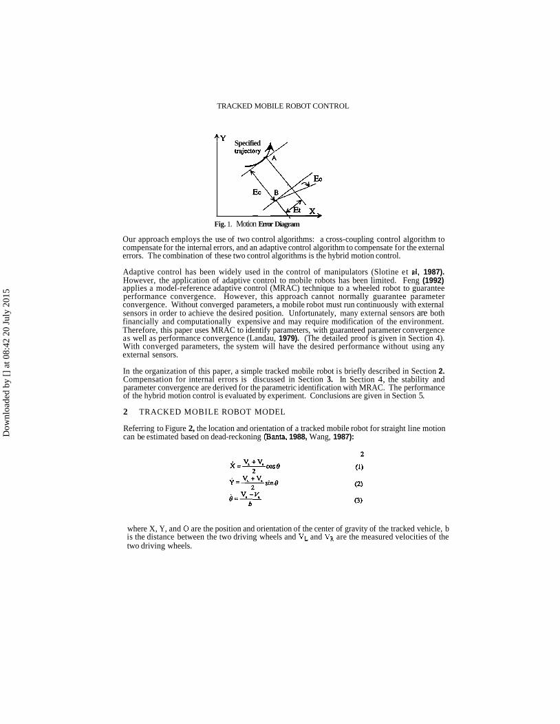
Motion errors can be decomposed into orientation errors, contour errors, and tracking errors as shown in Figure 1. The vehicle is instructed at point A, but it is at point B. The orientation error EO is defined as the angular difference between the actual orientation and the desired orientation. The contour error E, is the distance between the actual position B and the desired trajectory in the direction perpendicular to the direction of travel. The tracking error E,is the distance between the actual position and the desired position in the direction of travel. In mobile robot motion control, the orientation errors are the dominant errors since they cause unbounded growth of the contour errors. The tracking errors are usually of less concern (Feng. 1992).

Dow

nloa

ded

by [

] at

08:

42 2

0 Ju

ly 2

015

TRACKED MOBILE ROBOT CONTROL

Specified trajdov &

Fig. 1. Motion Error Diagram

Our approach employs the use of two control algorithms: a cross-coupling control algorithm to compensate for the internal errors, and an adaptive control algorithm to compensate for the external errors. The combination of these two control algorithms is the hybrid motion control.

Adaptive control has been widely used in the control of manipulators (Slotine et al, 1987). However, the application of adaptive control to mobile robots has been limited. Feng (1992) applies a model-reference adaptive control (MRAC) technique to a wheeled robot to guarantee performance convergence. However, this approach cannot normally guarantee parameter convergence. Without converged parameters, a mobile robot must run continuously with external sensors in order to achieve the desired position. Unfortunately, many external sensors are both financially and computationally expensive and may require modification of the environment. Therefore, this paper uses MRAC to identify parameters, with guaranteed parameter convergence as well as performance convergence (Landau, 1979). (The detailed proof is given in Section 4). With converged parameters, the system will have the desired performance without using any external sensors.

In the organization of this paper, a simple tracked mobile robot is briefly described in Section 2. Compensation for internal errors is discussed in Section 3. In Section 4, the stability and parameter convergence are derived for the parametric identification with MRAC. The performance of the hybrid motion control is evaluated by experiment. Conclusions are given in Section 5.

2 TRACKED MOBILE ROBOT MODEL

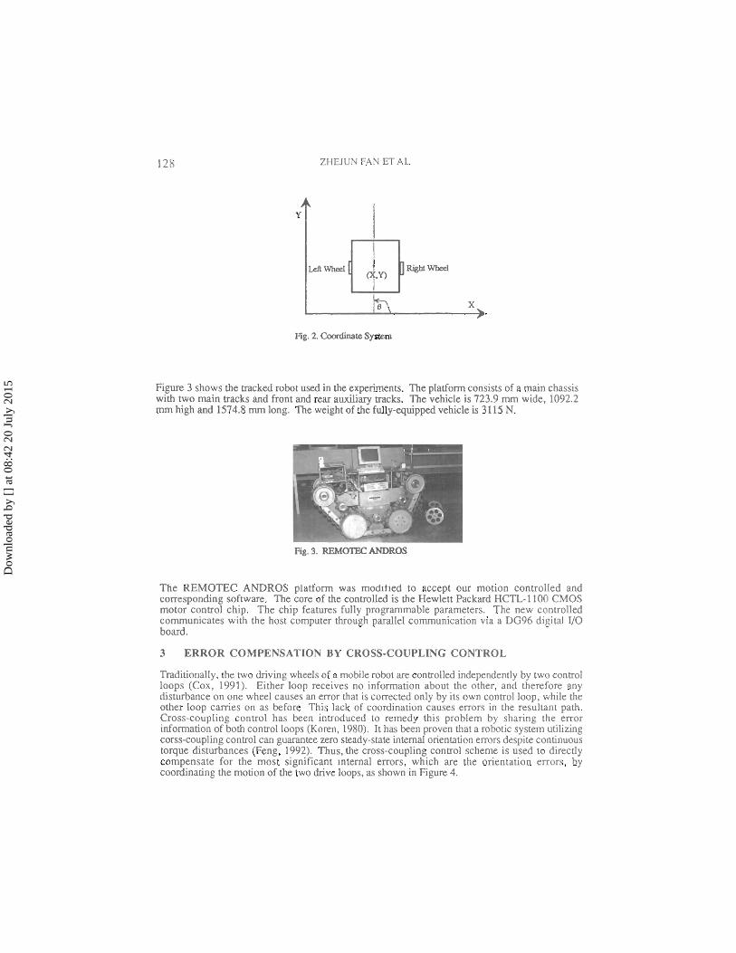
Referring to Figure 2, the location and orientation of a tracked mobile robot for straight line motion can be estimated based on dead-reckoning (Banta, 1988, Wang, 1987):

where X, Y, and 0 are the position and orientation of the center of gravity of the tracked vehicle, b is the distance between the two driving wheels and VL and VR are the measured velocities of the two driving wheels.

Dow

nloa

ded

by [

] at

08:

42 2

0 Ju

ly 2

015

128 ZHEJUN FAN ET AL

Wg. 2. Coordinale System

Figure 3 shows the hacked robot used in the experiments. The platform consists of a main chassis with two main tracks and front and rear auxiliary tracks. The vehicle is 723.9 mm wide, 1092.2 mm high and 1574.8 mm long. The weight of the fully-quipped vehicle is 3115 N.

Fig. 3. REMOTEC ANDROS

The REMOTEC ANDROS platform was modified to accept our motion controlled and corresponding software. The core of the controlled is the Hewlett Packard HCTL-1100 CMOS motor control chip. The chip features fully programmable parameters. The new controlled communicates with the host computer through parallel communication via a DG96 digital I/O board.

3 ERROR COMPENSATION BY CROSS-COUPLING CONTROL

Traditionally, the two driving wheels of a mobile robot are controlled independently by two control loops (Cox, 1991). Either loop receives no information about the other, and therefore any disturbance on one wheel causes an error that is corrected only by its own control loop, while the other loop carries on as before This lack of coordination causes errors in the resultant path. Cross-coupling control has been inuoduced to remedy this problem by sharing the error information of both control loops (Koren, 1980). It has been proven that a robotic system utilizing corss-coupling conml can guarantee zero steady-state internal orientation errors despite continuous torque disturbances (Feng, 1992). Thus, the cross-coupling control scheme is used to directly compensate for the most significant internal errors, which are the orientation errors. by coordinating the motion of the two drive loops, as shown in Figure 4.

Dow

nloa

ded

by [

] at

08:

42 2

0 Ju

ly 2

015

TRACKED MOBILE ROBOT CONTROL

fig. 4. clD.scoupliog Cootr0ue-r

3.1 Steady-State Analysis

When the cross-coupling control loop has reached its steady state, we can apply final value theorem to this two input two output system and obtain an expression for the steady state value of

and wq, respectively.

where R, .R, = the right mi left whcel annmand velocities V, ,VL = the right and left whcel actual velocities m,.m, = the right and I& wheel angular velocities C, .CL = the right mi I& wheel canpermtian gains

K, .K, = the I& and right drive loop DC gains TL .T, = the left and right drive loop time wnstauts

r = 146 mm, the assumed nominal wheel radius for both I& and right drive loop

r, ,r, = the actual left and right wheel radii

K, ,K, = the proportional and integral gains for a PI controller

The sampling time for the cross-coupling control loop only is about 30 ms. Since the sampling time for the adaptive control loop is 500 ms, as it requires two additional ultrasonic sensors to measure the external orientation of the mobile robot, (discussed in Section 4), it can be assumed that the cross-coupling controlled is at its steady state when adaptive control was applied later.

Dow

nloa

ded

by [

] at

08:

42 2

0 Ju

ly 2

015

ZHEJUN FAN ET AL.

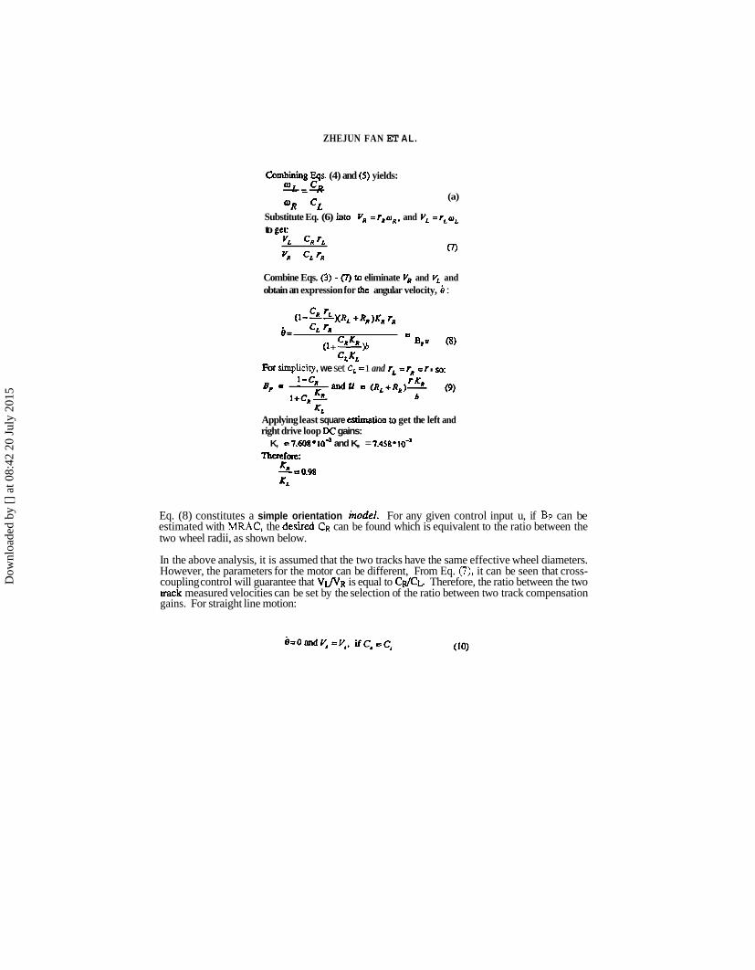
Combiming Egs. (4) and (5) yields: a~ - c ~ --- (a) OR c~

Substitute Eq. (6) into V, =r,,o,, and V, =r,a, to get

YL, CR r, 0

VR CL r,

Combine Eqs. (3) - (7) to eliminate V, and V, and obtain an expression for the angular velocity, i) :

( l - ~ ~ x ~ , +R& r,, i= CL 'R

CRKR Bpu (8) (1 + -9 CLKL

For simplicity, we set C, = 1 and rL = rn = r . SO:

- KL

Applying least square estimation to get the left and right drive loop DC gains:

K, = 7.608. lo4 and K,, = 7.458*10" 'Ibenfare:

L a 9 8 KL

Eq. (8) constitutes a simple orientation inodel. For any given control input u, if Bp can be estimated with MRAC, the desired CR can be found which is equivalent to the ratio between the two wheel radii, as shown below.

In the above analysis, it is assumed that the two tracks have the same effective wheel diameters. However, the parameters for the motor can be different, From Eq. (7). it can be seen that cross- coupling control will guarantee that V f l ~ is equal to CR/& Therefore, the ratio between the two track measured velocities can be set by the selection of the ratio between two track compensation gains. For straight line motion:

Dow

nloa

ded

by [

] at

08:

42 2

0 Ju

ly 2

015

TRACKED MOBILE ROBOT CONTROL 131

If the two wheel diameters are not the same. Eq. (8) can be set to zero to obtain the following equation:

then, V, = VL will be obtained if

Therefore, it can be concluded that for a straight-line motion, CR is equivalent to the ratio between r~ and r~ if we assume CL = 1. Parametric identification will be used to find CR.

3.2 Experimental Results for Cross-coupling Control

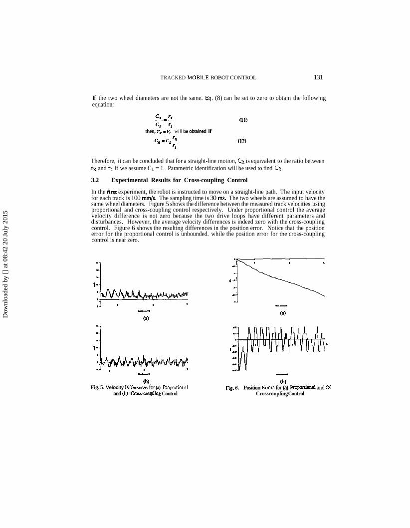
In the fnst experiment, the robot is instructed to move on a straight-line path. The input velocity for each track is 100 mm/s. The sampling time is 30 ms. The two wheels are assumed to have the same wheel diameters. Figure 5 shows the difference between the measured track velocities using proportional and cross-coupling control respectively. Under proportional control the average velocity difference is not zero because the two drive loops have different parameters and disturbances. However, the average velocity differences is indeed zero with the cross-coupling control. Figure 6 shows the resulting differences in the position error. Notice that the position error for the proportional control is unbounded. while the position error for the cross-coupling control is near zero.

r H

(3) Fig. 5. Velocity Diff- for (a) Roportional

and (b) Ctrssaupling Control

-u

@I Fig. 6. Position Emws for (a) Proportional and (b)

Crosscoupling Control

Dow

nloa

ded

by [

] at

08:

42 2

0 Ju

ly 2

015

ZHEJLIN FAN ET AL.

From the experimental results, it can be concluded that the proposed cross-coupling controller can more accurately control the robot by coordinating the motions in both drive loops in spite of different parameters and disturbances in the left and right motors. However, it cannot handle the external error such as the different effective wheel diameters.

4 COMPENSATION FOR EXTERNAL ERRORS BY ADAPTIVE CONTROL

The cross-coupling controller is very effective in compensating for the internal errors such as different parameters in the left drive loop and the right drive loop. It guarantees that the actual angular velocities of the left wheel and the right wheel are the same for a straight-line motion. However, if the two effective wheel diameters are different, the distances traveled by the two wheels will be different even though their angular velocities are the same, which will cause orientation error and consequently unbounded position errors. These are systematic external errors that cannot be compensated for by cross-coupling control. As shown in (Borenstein, 1992). a 1 rnrn deviation in the nominal 114 mrn wheel diameter can cause up to 8.3 degree orientation error and a 0.74 m lateral position error for a planned 10 m straight-line motion.

In order to compensate for the orientation errors due to different wheel diameters, parametric identification with model reference adaptive control can be used to estimate the parameter CR. The adaptive loop will use the orientation information measured by two sonars in real-time to estimate the internal parameters, and will result in smaller orientation errors.

4.1 Hyperstability Approach

The three basic approaches considered in the design of an' MRAC system were based on the use of local parametric optimization theory, Lyapunov function, and hyperstability (Landau, 1979). Among those approaches, hyperstability was selected since it allows the choice of a class of Lyapunov functions in order to widen the class of control laws which lead to a globally stable MRAC system.

The hyperstability approach starts by analyzing the stability of the system and then choosing the best adaptation gains from all the stable systems. The design procedure starts by transforming the MRAC system into the form of an equivalent feedback system composed of two blocks, one in the feedforward path and one in the feedback path. Then the solutions are found for the part of the adaptation laws that appears in the feedback path of the equivalent system so that the Popov integral inequality is satisfied. Then solutions are found for the remaining part of the adaptation law that appears in the feedforward path such that the feedforward path is a hyperstable block. Finally, the adaptation law is transformed back to the original MRAC system.

4.2 Main Concept

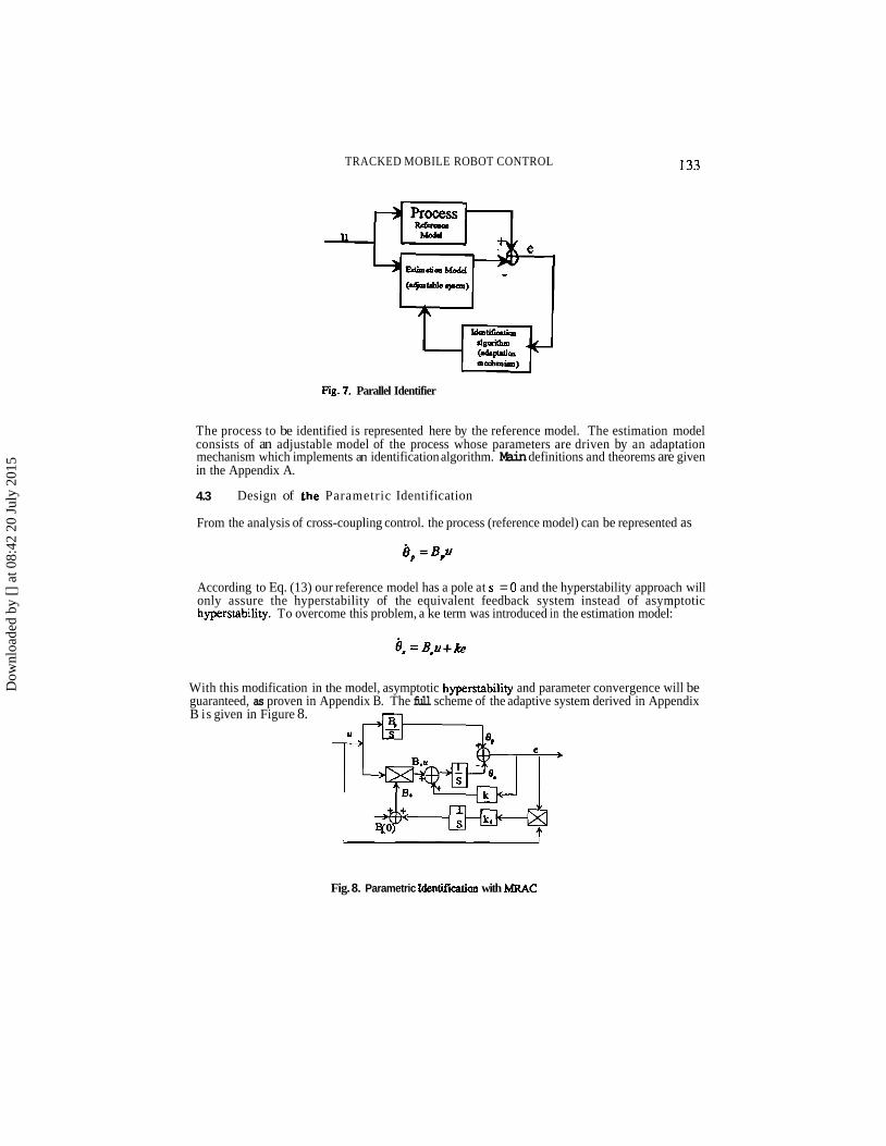
The objective is to find the ratio between the two effective wheel radii ( r ~ l r t ) in order to compensate for external errors. If Bp can be estimated, then CR can be found from Eq. (9). Parameter identification with MRAC is used to estimate Bp as shown in Figure 7.

Dow

nloa

ded

by [

] at

08:

42 2

0 Ju

ly 2

015

TRACKED MOBILE ROBOT CONTROL

fig. 7. Parallel Identifier

The process to be identified is represented here by the reference model. The estimation model consists of an adjustable model of the process whose parameters are driven by an adaptation mechanism which implements an identification algorithm. Main definitions and theorems are given in the Appendix A.

4.3 Design of the Parametric Identification

From the analysis of cross-coupling control. the process (reference model) can be represented as

According to Eq. (13) our reference model has a pole at s = 0 and the hyperstability approach will only assure the hyperstability of the equivalent feedback system instead of asymptotic hyperstability. To overcome this problem, a ke term was introduced in the estimation model:

With this modification in the model, asymptotic hyperstability and parameter convergence will be guaranteed, as proven in Appendix B. The full scheme of the adaptive system derived in Appendix B is given in Figure 8.

Fig. 8. Parametric Identification with MRAC

Dow

nloa

ded

by [

] at

08:

42 2

0 Ju

ly 2

015

134 ZHEJUN FAN E T A L

4.4 Adaptive Controlled Hardware

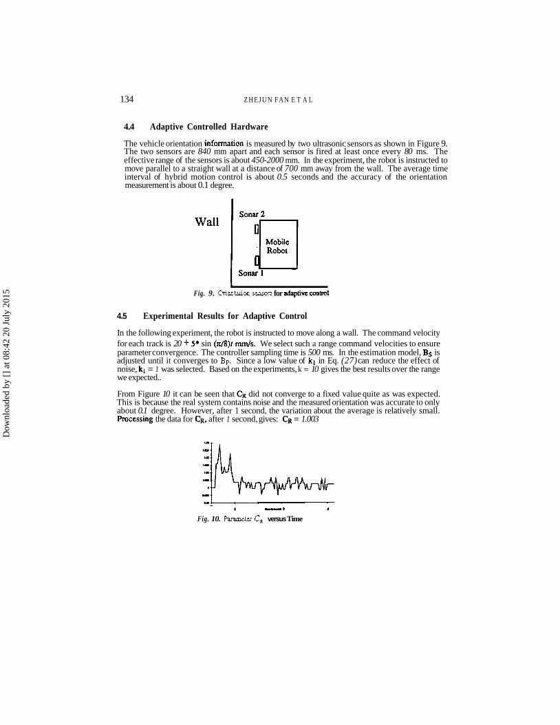
The vehicle orientation information is measured by two ultrasonic sensors as shown in Figure 9. The two sensors are 840 mm apart and each sensor is fired at least once every 80 ms. The effective range of the sensors is about 450-2000 mm. In the experiment, the robot is instructed to move parallel to a straight wall at a distance of 700 mm away from the wall. The average time interval of hybrid motion control is about 0.5 seconds and the accuracy of the orientation measurement is about 0.1 degree.

Fig. 9. OrieIltaIioo sensors for adaptive coornl

4.5 Experimental Results for Adaptive Control

In the following experiment, the robot is instructed to move along a wall. The command velocity for each track is 20 + 5* sin (nl8)t 4 s . We select such a range command velocities to ensure parameter convergence. The controller sampling time is 500 ms. In the estimation model, Bs is adjusted until it converges to Bp. Since a low value of kl in Eq. (27) can reduce the effect of noise, kl = 1 was selected. Based on the experiments, k = 10 gives the best results over the range we expected..

From Figure 10 it can be seen that CR did not converge to a fixed value quite as was expected. This is because the real system contains noise and the measured orientation was accurate to only about 0.1 degree. However, after 1 second, the variation about the average is relatively small. hocessing the data for CR, after 1 second, gives: CR = 1.003

I L U I a

Fig. 10. Parametu CR versus Time

Dow

nloa

ded

by [

] at

08:

42 2

0 Ju

ly 2

015

TRACKED MOBILE ROBOT CON'TROL 135

Since the nominal wheel diameter is 292 mrn for the tracked mobile robot, there is a 0.876 mm difference between the two effective wheel diameters.

In order to check the accuracy of this identified parameter, the hxcked vehicle was made to move 4 m in a straight-line path 10 times, with the parameter CR identified by hybrid control. For comparison, we repeated the experiment with cross-coupling control only. The results are shown in Table 1.

Table I

The results shown in Table 1 demonstrate that hybrid control is much better than regular cross- coupling control alone. Even with this identified parameter, the error is not zero due to noise, sensor inaccuracies, and unmodeled dynamics.

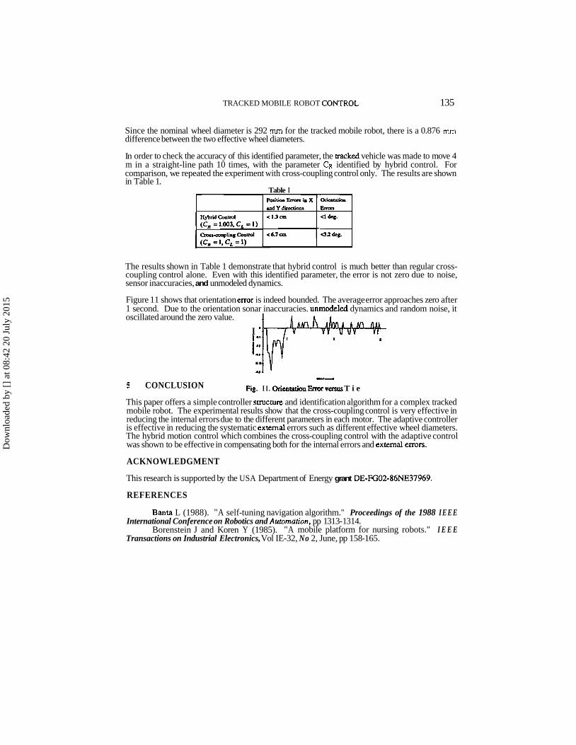
Figure 11 shows that orientation error is indeed bounded. The average error approaches zero after 1 second. Due to the orientation sonar inaccuracies. unmodeled dynamics and random noise, it oscillated around the zero value.

I ' i r .. .. .. 5 CONCLUSION

w-

fig. I I . Orientation E m v m T i e

This paper offers a simple controller saucture and identification algorithm for a complex tracked mobile robot. The experimental results show that the cross-coupling control is very effective in reducing the internal errors due to the different parameters in each motor. The adaptive controller is effective in reducing the systematic extemal errors such as different effective wheel diameters. The hybrid motion control which combines the cross-coupling control with the adaptive control was shown to be effective in compensating both for the internal errors and extemal errors.

ACKNOWLEDGMENT

This research is supported by the USA Department of Energy grant DE-FG02-86NE37969.

REFERENCES

Banta L (1988). "A self-tuning navigation algorithm." Proceedings of the 1988 IEEE International Conference on Robotics and Automation, pp 13 13- 13 14.

Borenstein J and Koren Y (1985). "A mobile platform for nursing robots." I E E E Transactions on Industrial Electronics, Vol IE-32, No 2, June, pp 158-165.

Dow

nloa

ded

by [

] at

08:

42 2

0 Ju

ly 2

015

136 ZHEJUN FAN ET AL.

Borenstein J (1992). Mobile Robot Course Pack, Ann Arbor, The University of Michigan. Cox IJ (1991). "Blanche--an experiment in guidance and navigation of an autonomous

robot vehicle." IEEE Transactions on Robotics and Automation, Vol7, No 2, April, pp 193-204. Feng L (1992). "Adaptive motion control of mobile robot." Ph.D. thesis, The University

of Michigan. Koren Y (1980). "Cross-coupling biaxial computer conh-01 for manufacturing systems."

ASME Journal on Dynamic System, Measurement, and Control, Vol 102, Dec, pp 265-272. Landau YD (1979). Aduptive Control. Marcel Dekker, Inc., New York. Slotine J-JE, Li W (1987). "On the adaptive control of robot manipulators." ~ n t ' ~

Robotics Res, 6 , 3. Wang CM (1987). "Location estimation and error analysis for an autonomous mobile

robot." GMR-5897, General Motors Research Laboratories, Warren, Michigan 48090, July 9, 1987.

Wong JY, Preston-Thomas J (1984). "A comparison between a conventional method and an improved method for predicting tracked vehicle performance." Proceedings of the 8th International Conference of the International Society for Terrain-Vehicle Systems, Vienna, Austria, Nov.

APPENDIX A

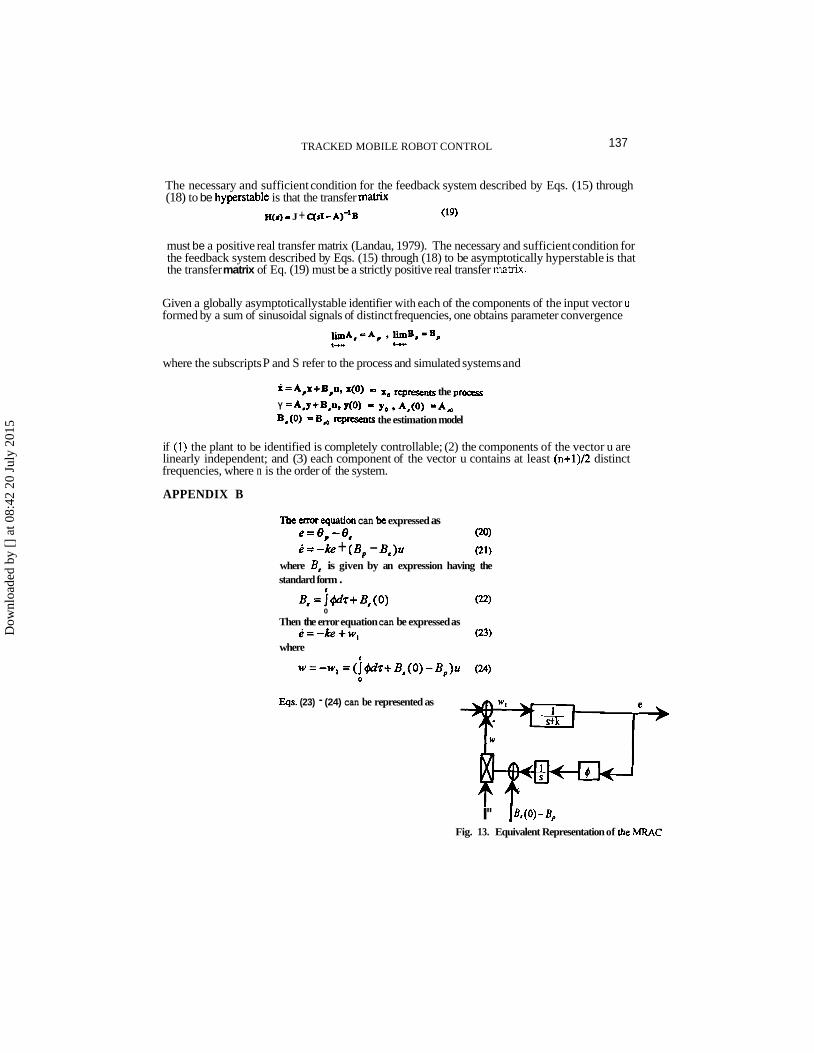
In order to prove the global stability and parameter convergence, consider the feedback system depicted in Figure 12. The system is formed by a linear time-invariant feedforward block and feedback block which can be linear or nonlinear and time-invariant or time-varying.

Fig. 12 Nonlinear Feedback System

The feedback system represented in Figure 12 is termed (asymptotically) hyperstable if it is (asymptotically) globally stable with aU the feedback blocks satisfying Popov integral inequality. Eq . (15):

t t ) d for all 4 > b (15) 1.

Consider the closed system having a feedfornard block

i=Ax+Bu=Ax-Bw (16) v = Cx+ Ju= Cx- Jw (17)

and a feedback block w = f(v,t) (18)

which satisfies the Popov inregml incqualify

Dow

nloa

ded

by [

] at

08:

42 2

0 Ju

ly 2

015

TRACKED MOBILE ROBOT CONTROL 137

The necessary and sufficient condition for the feedback system described by Eqs. (15) through (18) to be hyperstable is that the transfer mahix

~ ( s ) = J + q d -A)-'B (19)

must be a positive real transfer matrix (Landau, 1979). The necessary and sufficient condition for the feedback system described by Eqs. (15) through (18) to be asymptotically hyperstable is that the transfer matrix of Eq. (19) must be a strictly positive real transfer matrix.

Given a globally asymptotically stable identifier with each of the components of the input vector u formed by a sum of sinusoidal signals of distinct frequencies, one obtains parameter convergence

where the subscripts P and S refer to the process and simulated systems and

i =A,x+B,u. ~ ( 0 ) I, rcpmsents the prazrs Y =A,y+B,u, ~ ( 0 ) = y o . A,(O) =A, B, (0) a B, rcpmenfs the estimation model

if (1) the plant to be identified is completely controllable; (2) the components of the vector u are linearly independent; and (3) each component of the vector u contains at least (n+1)/2 distinct frequencies, where n is the order of the system.

APPENDIX B

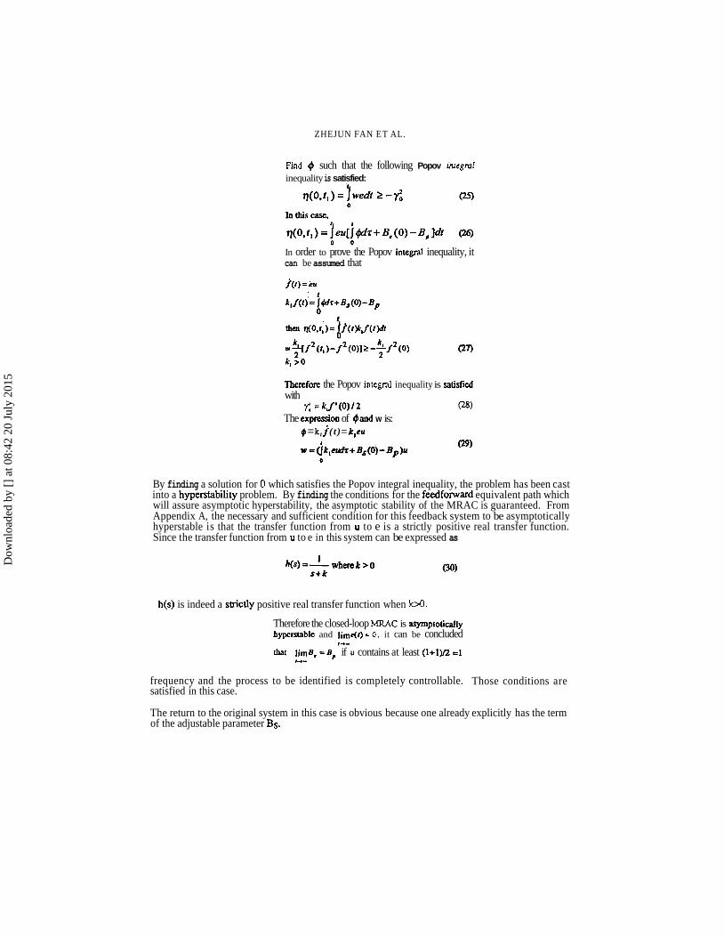
The uror equation can be expressed as e = 8 , - 8 , (20)

i = -ke + (B, - B,)u (21) where B, is given by an expression having the standard form .

B; = j c ) d r + ~ ; ( 0 ) (22) 0

Then the error equation can be expressed as e = - k e + w , (23)

where

Eqs. (23) - (24) can be represented as

I" ]B.(o)-B, Fig. 13. Equivalent Representation of the MRAC

Dow

nloa

ded

by [

] at

08:

42 2

0 Ju

ly 2

015

ZHEJUN FAN ET AL.

Find 4 such that the following Popov inregml inequality is satisfied:

. .

In order to prove the Popov integral inequality, it can be assumed that

Therefore the Popov integral inequality is satisfi with

r', = k,f1(0)/2 (zs)

The exp&on of #and w is: # = k, f ( t ) = k,eu

By finding a solution for 0 which satisfies the Popov integral inequality, the problem has been cast into a hyperstability problem. By finding the conditions for the feedforward equivalent path which will assure asymptotic hyperstability, the asymptotic stability of the MRAC is guaranteed. From Appendix A, the necessary and sufficient condition for this feedback system to be asymptotically hyperstable is that the transfer function from u to e is a strictly positive real transfer function. Since the transfer function from u to e in this system can be expressed as

h(s) is indeed a strictly positive real transfer function when k>O.

Therefore the closed-loop MRAC is asymptotically hyperstable and lim41) = 0. it can be concluded

1 4 -

Lbat IimB, =B, if u contains at least (l+l)~% r l 1 4 -

frequency and the process to be identified is completely controllable. Those conditions are satisfied in this case.

The return to the original system in this case is obvious because one already explicitly has the term of the adjustable parameter Bs.

Dow

nloa

ded

by [

] at

08:

42 2

0 Ju

ly 2

015