tracer testing in the svartsengi geothermal field in

Tracer testing in the Svartsengi geothermalfield in 2015

Sigrún Brá Sverrisdóttir

Thesis of 60 ECTS creditsMaster of Science (M.Sc.) in Sustainable Energy

Engineering

January 2016

Tracer testing in the Svartsengi geothermal field in 2015

Thesis of 60 ECTS credits submitted to the School of Science and Engineeringat Reykjavík University in partial fulfillment of

the requirements for the degree ofMaster of Science (M.Sc.) in Sustainable Energy Engineering

January 2016

Supervisors:

Ágúst Valfells, SupervisorAssociate Professor, Reykjavík University, Iceland

Guðni Axelsson, Co-advisorReservoir Engineer, ÍSOR, Iceland

Examiner:

Egill Júlíusson, ExaminerReservoir Engineer, Landsvirkjun, Iceland

CopyrightSigrún Brá Sverrisdóttir

January 2016

Tracer testing in the Svartsengi geothermal field in2015


January 2016

AbstractThe Svartsengi geothermal field has been utilized for district heating since 1976and electricity generation since 1980. Some complications due to the utilizationhave arisen throughout the years. Those include a rapid pressure drawdown inthe field and issues regarding waste water management. The continuous injectionof spent geothermal fluid began in 1998 when SV-17 was taken into use. Withthe addition of SV-24 as an injection well in 2008, the injection rate was slowlyincreased to 60% of the extraction rate. Pressure measurements showed that theinjection provided pressure support to the field, but the addition of a new energyplant and increased production from the field reintroduced the trend of decliningfield pressure. An important part of geothermal field management is to monitorinjection wells and study the ability to increase reinjection. In the summer of 2015a threefold tracer test was performed in Svartsengi for that purpose. Liquid phasetracers were injected into wells SV-17 and SV-24, 2,7-napthalene disulfonate and2,6-napthalene disuldonate, and a steam tracer, sulfurhexafluoride, was injected intoSV-24. Samples have since been taken from all production wells in the field withthe addition of the monitoring well in Eldvörp. At the time of writing the 2,6-NDShas only been detected in well SV-9, while no signs have been noted of 2,7-NDS.However, the steam tracer has been detected in all production wells and samplingfor that has been terminated, but no signs were detected in the well in Eldvörp.The tracer returns were modelled quantitatively using a couple of programs fromthe ICEBOX software package from ÍSOR. TRINV was used to simulate the tracerrecovery based on the theory of solute transport and one dimensional flow channelmodels. TRCOOL was used to predict the cooling in the production wells dueto the injection. Only 0.035% of the injected steam phase tracer was recoveredin the production wells, indicating a very modest recharge from the injection wellto the production wells. Well SV-23 had the largest tracer recovery, but SV-11experienced the highest tracer concentration. Cooling predictions were calculatedfor the current injection scenario in well SV-24 and for a scenario where the currentinjection rate was doubled, for 30 years. For both scenarios the model predicted aninsignificant cooling in production wells over the 30 year period.

Úrvinnsla á ferilefnaprófunum í Svartsengi 2015


janúar 2016

ÚtdrátturVinnsla úr jarðhitasvæðinu Svartsengi hófst árið 1976 þegar heitu vatni var hleyptá fyrstu húsin í Grindavík. Fjórum árum síðar hófst raforkuframleiðsla úr svæðinu,þegar orkuver III var tekið í notkun. Með stöðugri framleiðslu hafa nokkur stærrivandmál litið dagsins ljós. Þar á meðal má nefna; hröð þrýstingslækkun vegnavinnslu og losun jarðsjávar á yfirborð. Til að stemma stigu við þessum vandamál-um hófst stöðug niðurdæling í holu SV-17 árið 1998. Tíu árum seinna var annarriniðurdælingarholu bætt við, SV-24, og í hægum skrefum var niðurdæling aukin í60% af upptöku úr svæðinu. Þrýstingsmælingar sýndu að niðurdælingin dró veru-lega úr hraða þrýstingslækkunarinnar í vinnsluholum, en þegar orkuver VI tók tilstarfa jókst þrýstingslækkun í Svartsengi á ný. Hluti af rekstri jarðhitasvæða er aðrannsaka áhrif niðurdælingar á svæðið og kanna möguleika á aukinni niðurdælingu.Í þeim tilgangi hófst þríþátta ferilefnapróf sumarið 2015. Vökvafasa ferilefni vorusett niður í holur SV-17 og SV-24, 2,7-napthalene disulfonate og 2,6-napthalenedisulfonate. Gufufasa ferilefnið sulfuhexafluoríð var sett niður í holu SV-24. Sýnivoru síðan tekin úr öllum vinnslu holum í Svartsengi ásamt rannsóknar holu í Eld-vörp. Þegar þetta er skrifað, hefur vökvafasa ferilefnið sem sett var niður í holuSV-24 einungis greinst í tveimur sýnum frá einni holu, SV-9, en gufufasa efnið hefurlokið komu sinni í allar vinnsluholur. Enn hefur ekki greinst 2,7-napthalene disul-fonat. Engin merki um sulfurhexafluoríð voru merkjanleg í Eldvörp. Endurheimturgufufasans voru hermdar í forritum sem fáanleg eru í ICEBOX forritapakkanum fráÍSOR. TRINV var notað til að herma rennslisleiðir milli niðurdælingar holunnarog vinnsluholanna. TRCOOL var hinsvegar notað til að reikna út áætlaða kólnunsvæðisins vegna niðurdælingar. Einungis 0,035% af ferlefninu sem var dælt niðurvar endurheimt í vinnsluholunum. Það benti til þess að einungis örlítill hluti afniðurdældavökvanum skilaði sér í þær holur sem vinna úr gufuhluta svæðisins.Stærsti hluti ferilefnisins var endurheimtur í holu SV-23, en hæsti styrkur efnisinskom fram í holu SV-11. Gerðar voru kólnunarspár fyrir núverandi niðurdælingu í30 ár, ásamt tvöföldu magni þess sem nú er dælt niður. Báðar spár bentu til þess aðniðurdæling í 30 ár myndi ekki hafa marktæk áhrif á núverandi hitastig svæðisins.

Tracer testing in the Svartsengi geothermal field in 2015


Thesis of 60 ECTS credits submitted to the School of Science and Engineeringat Reykjavík University in partial fulfillment of

the requirements for the degree ofMaster of Science (M.Sc.) in Sustainable Energy Engineering

January 2016

Student:


Supervisors:

Ágúst Valfells

Guðni Axelsson

Examiner:

Egill Júlíusson

The undersigned hereby grants permission to the Reykjavík University Library to reproducesingle copies of this Thesis entitled Tracer testing in the Svartsengi geothermal field in2015 and to lend or sell such copies for private, scholarly or scientific research purposes only.The author reserves all other publication and other rights in association with the copyrightin the Thesis, and except as herein before provided, neither the Thesis nor any substantialportion thereof may be printed or otherwise reproduced in any material form whatsoeverwithout the author’s prior written permission.

date

Sigrún Brá SverrisdóttirMaster of Science

Acknowledgements

I would like to acknowledge Ágúst Valfells and Guðni Axelsson for their support and guid-ance throughout this whole process, and my employer HS Orka for trusting me with thisproject and providing me with all the resources needed to finish the thesis, both financialand informations, Kristín Vala Matthíasdóttir for bringing me the idea this project and all theencouragement throughout the process, Ómar Sigurðsson for working on production num-bers and providing valuable feedback, and KjartanMarteinsson for assisting me with TRINV.

Finally, I want to thank my family for all the support when I needed it the most andspecial thanks to my boyfriend Rich for his endless support and proofreading.

xvii

Contents

Acknowledgements xv

Contents xvii

List of Figures xix

List of Tables xxi

List of Abbreviations xxiii

List of Symbols xxv

1 Introduction 11.1 Aim and objectives . . . . . . . . . . . . . . . . . . . . . . . . . . . . . . 2

2 Background 32.1 Tracer tests . . . . . . . . . . . . . . . . . . . . . . . . . . . . . . . . . . 32.2 The geological setting of Svartsengi . . . . . . . . . . . . . . . . . . . . . 5

2.2.1 Hydrological connection between Svartsengi and Eldvörp . . . . . . 62.2.2 Conceptual model of Svartsengi . . . . . . . . . . . . . . . . . . . 7

2.3 The injection history of Svartstengi . . . . . . . . . . . . . . . . . . . . . . 162.4 Tracer tests in the Svartsengi geothermal field . . . . . . . . . . . . . . . . 18

3 Methods 233.1 Sampling methods . . . . . . . . . . . . . . . . . . . . . . . . . . . . . . . 24

3.1.1 Vapor phase sampling methods . . . . . . . . . . . . . . . . . . . . 243.1.2 Liquid phase sampling methods . . . . . . . . . . . . . . . . . . . 25

3.2 Analytical methods . . . . . . . . . . . . . . . . . . . . . . . . . . . . . . 273.2.1 Vapor phase sample analytical methods . . . . . . . . . . . . . . . 273.2.2 Liquid phase analytical methods . . . . . . . . . . . . . . . . . . . 29

3.3 Modeling methods . . . . . . . . . . . . . . . . . . . . . . . . . . . . . . . 293.3.1 Tracer transport . . . . . . . . . . . . . . . . . . . . . . . . . . . . 303.3.2 Thermal breakthrough . . . . . . . . . . . . . . . . . . . . . . . . 31

4 Results 354.1 Tracer recovery . . . . . . . . . . . . . . . . . . . . . . . . . . . . . . . . 354.2 Modeling . . . . . . . . . . . . . . . . . . . . . . . . . . . . . . . . . . . 39

4.2.1 Steam phase tracer returns . . . . . . . . . . . . . . . . . . . . . . 394.2.1.1 Analysis of two phase wells . . . . . . . . . . . . . . . . 394.2.1.2 Analysis of steam zone wells . . . . . . . . . . . . . . . . 42

xviii

4.2.2 Liquid phase tracer returns . . . . . . . . . . . . . . . . . . . . . . 464.3 Cooling predictions . . . . . . . . . . . . . . . . . . . . . . . . . . . . . . 47

5 Conclusions 495.1 Recommendations . . . . . . . . . . . . . . . . . . . . . . . . . . . . . . . 51

Bibliography 53

xix

List of Figures

2.1 Main tectonic features at Reykjanes Peninsula. Fissure swarms from Sæmunds-son (1978) shown as yellow shaded areas [19], modified from Jenness andClifton[20]. . . . . . . . . . . . . . . . . . . . . . . . . . . . . . . . . . . . . . . . . 6

2.2 Estimated reservoir temperature at 600 meters below sea level. Modified fromGerorgsson and Tulinius [22] by Vatnaskil [19]. . . . . . . . . . . . . . . . . . 7

2.3 Measured volcanic intrusions, modified by Vatnaskil from Franzson [26], [19]. . 82.4 Geologic cross-section at Svartsengi showing sequence of lava and hyaloclastite

layers, intrusive rock, faults and proposed flow patterns within geothermal andgroundwater aquifers. Modified by Vatnaskil from Franzson [19], [26]. . . . . . 9

2.5 A possible model of the steam zone at Svartsengi [27]. . . . . . . . . . . . . . 102.6 A comparison of geological cross-section in wells SV-18 and SV-19 to figure 2.4

[28]. . . . . . . . . . . . . . . . . . . . . . . . . . . . . . . . . . . . . . . . . 112.7 Location of production wells at Svartsengi, direction of directionally drilled

wells shown in red. Modified from [7]. . . . . . . . . . . . . . . . . . . . . . . 122.8 Subsidence rate at the outer part of the Reykjanes peninsula for four time inter-

vals. Bench marks are shown by solid circles, roads are shown by thick lines,contour intervals are 1 mm/year [37]. . . . . . . . . . . . . . . . . . . . . . . . 15

2.9 Location of main fussure swarms and earthquake belt on Reykjanes peninsula,modified from Kjaran et al., 1980 [19], [24]. . . . . . . . . . . . . . . . . . . . 15

2.10 Pressure at 900 m depth in Svartsengi and Eldvörp from 1980-2013 [7]. . . . . 172.11 Sodium concentration in well SV-6, SV-9 and SV-10 [38]. . . . . . . . . . . . . 192.12 Percentage of carbondioxide and nitrogen in gas in wells SV-6, SV-8, SV-9,

SV-10 and SV-11 [38]. . . . . . . . . . . . . . . . . . . . . . . . . . . . . . . 20

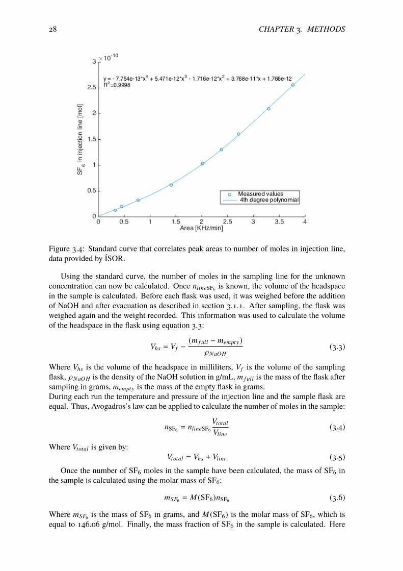
3.1 Webre seperator at wellhead for vapor phase sampling. . . . . . . . . . . . . . 253.2 Sampling set up, bottle upside down and water for cooling. . . . . . . . . . . . 263.3 Separator for liquid phase sampling. . . . . . . . . . . . . . . . . . . . . . . . 263.4 Standard curve that correlates peak areas to number of moles in injection line,

data provided by ÍSOR. . . . . . . . . . . . . . . . . . . . . . . . . . . . . . . 283.5 Diagram of an idealized single fracture matrix system [54]. . . . . . . . . . . . 33

4.1 Production variations throughout the steam phase test . . . . . . . . . . . . . . 364.2 Steam phase production for wet steam wells . . . . . . . . . . . . . . . . . . . 374.3 Concentration of SF6 in production wells . . . . . . . . . . . . . . . . . . . . 384.4 Cumulative SF6 returns per well . . . . . . . . . . . . . . . . . . . . . . . . . 384.5 Observed and simulated SF6 recovery in well SV-11 . . . . . . . . . . . . . . . 404.6 Observed and simulated SF6 recovery in well SV-7 . . . . . . . . . . . . . . . 414.7 Observed and simulated SF6 recovery in well SV-22 . . . . . . . . . . . . . . . 424.8 Observed and simulated SF6 recovery in well SV-23. . . . . . . . . . . . . . . 43

xx

4.9 Observed and simulated SF6 recovery in well SV-10. . . . . . . . . . . . . . . 444.10 Observed and simulated SF6 recovery in well SV-16. . . . . . . . . . . . . . . 454.11 Observed and simulated SF6 recovery in well SV-20 . . . . . . . . . . . . . . . 46

xxi

List of Tables

2.1 Information about well depth and distances from reinjection wells. . . . . . . . 14

3.1 Sampling schedule for both SF6 and NDS. . . . . . . . . . . . . . . . . . . . . 23

4.1 Parameters of the flow channel model simulating the tracer recovery in well SV-11. 404.2 Parameters of the flow channel model simulating tracer recovery in well SV-7. . 414.3 Parameters of the flow channel model simulating tracer recovery in well SV-22. 424.4 Parameter of the flow channel model simulating tracer recovery in well SV-23 . 434.5 Parameter of the flow channel model simulating tracer recovery in well SV-10 . 444.6 Parameter of the flow channel model simulating tracer recovery in well SV-16. . 454.7 Parameter of the flow channel model simulating tracer recovery in well SV-20. . 464.8 Recommended assumptions for cooling predictions. . . . . . . . . . . . . . . . 474.9 Flow channel model parameters used to predict cooling. . . . . . . . . . . . . . 48

xxiii

List of Abbreviations

HPLC High performance liquid chromatographÍSOR Iceland GeoSurveyNDS Napthalenedisulfonateppb Parts per billionppm Parts per million

xxv

List of Symbols

Symbol DescriptionA Cross-sectional area of flow channel [m2]b Half of the fracture width [meters]C Tracer concentration [kg/m3]c f Specific heat of fracture zone material [J/kg/°C]cm Specific heat of rock matrix [J/kg/°C]cR Specific heat capacity of the rock [J/kg/°C]cw Specific heat of the geothermal fluid [J/kg/°C]c(t) Tracer concentration in produced fluid [kg/m3]C(t) Tracer concentration in flow channel [kg/m3]c(s) Tracer concentration in well [kg/L]D∗ Coefficient of molecular diffusion [m2/s]D Dispersion coefficient [m2/s]Fx Tracer mass flow rate, x-direction [kg/m2s]Fx,advection Tracer mass flow rate due to advection [kg/m2s]Fx,dispersion Tracer mass flow rate due to dispersion [kg/m2s]h Height of fracture [m]h f Enthalpy of saturated liquid [kJ/kg]hg Enthalpy of saturated vapor [kJ/kg]hgeo f Enthalpy of the geothermal fluid [kJ/kg]kth Thermal conductivity of the formation [W/m/°C]L Flow channel length [m]mempty Mass of an empty flask [g]mevacuated Mass of flask after evacuation [g]m f ull Mass of a full flask [g]mSF6 Mass of SF6mi (t) Cumulative tracer return [kg]M Injected tracer mass [kg]M (SF6) Molar mass of SF6 [g/mol]nline Number of moles in injection line [mol]nSF6 Number of SF6 moles in sample [mol]ntotal Total number of moles in sample [mol]Pline Pressure in injection line [mbar]q Flow in channel [kg/s]qin j Injection rate [kg/s]Q Production rate [kg/s]R Gas constant [83144.7 ml mbar /mol/K]Rthermal Thermal retardation coefficient [-]t Time [seconds]

xxvi

T f Temperature of fluid [°C]TI Initial formation temperature [°C]Tm Temperature of fluid in fracture [°C]Tp(L, t) Production temperature[°C]T0 Initial formation temperature [°C]T Temperature in sampling line [K]u Average linear velocity [m/s]Vf Volume of sampling flask [ml]Vhs Volume of flask headspace [ml]Vline Volume of intake line [l]Vtotal Total volume in gas chromatograph [l]x Distance along a flow channel [m]xv Vapor quality [-]

αL Longitudinal dispersivity of channel [m]αx Dispersivity [m]φ Porosity [-]ρ Density of material [kg/m3]π Piκ Thermal diffusivity [m2/s]ωin j Fraction of injected fluid reaching the production well [-]

1

Chapter 1

Introduction

The first wells were drilled in the Svartsengi geothermal field in 1971 and continuous useof the area was started 5 years later [1]. Early on, a rapid pressure draw down was noticedin the field and discussion about reinjecting fluid back into the system started [2]. A coupleof reinjection and tracer tests were done in the early 1980’s to test the field’s reaction toinjection. The tests in the early 1980’s showed that injection into well SV-12 would providepressure support to the system and reduce drawdown. However, due to its proximity toproduction wells, a rapid cooling in production wells would be expected in the field, and thewell was deemed too close to the production zone to serve as an injection well. Between1988 and 2000, injection, mostly of experimental nature, were performed into wells SV-5and SV-6. Like SV-12, these wells were located within the production zone causing a highrisk of a premature cold front in production wells. In 1998 well SV-17 was drilled about 2.4kmWSW of the production zone with the main purpose to serve as an injection well. In 2001injection started slowly at a rate of about 24 kg/s, but in 2014 the injection rate reached anall time maximum of 190 kg/s [3]. In late 2008 well SV-24 was added as a second injectionwell and currently HS Orka is reinjecting about 60% of the fluid that is being extracted fromthe field back into the system [4], [5],[6]. In addition to the reinjection by HS Orka, 100 kg/sof cold water was flowing into the system through a feed point at about 350 m depth in wellSV-24 between 2008-2010 [7]. Measurements have shown that the increased reinjection hasprovided a noticeable pressure support to the system. Pressure remained relatively constantfrom 2002 to 2008. In early 2008, energy plant VI, a 30 MW steam turbine, went into op-eration and despite the additional reinjection into SV-24 a pressure drawdown of 1 bar/yearhas been noted in the field since 2010 [8], [9].

The connections between the present injection wells and the production wells have neverbeen studied, and possible effects due to the injection are still unknown. Tracer tests havelong been used in hydrological systems, including geothermal fields, to study flow patternsand connections between wells. An important factor of geothermal field operation is propermanagement of reinjection. A cold front due to reinjection can cause large damage to a field,while on the other hand, large scale production where recharge is less than production cancause a rapid pressure decline in the field. In order to gain a better understanding of thesystem, HS Orka initiated a series of tracer tests in the summer of 2015. These tracer testswill be used to analyze connections between production wells and injection wells, predictlong term cooling in the field due to current reinjection, and estimate cooling due to higherand lower injection rates.

2 CHAPTER 1. INTRODUCTION

1.1 Aim and objectivesIn this paper I aim to answer a few questions that can help improve the management of theSvartsengi geothermal field and I will make recommendations on which parts of this tracertest could have been performed in a better way.The Svartsengi geothermal field has been managed successfully without major decline inproduction up to this day but more knowledge can lead to even longer lifetime of the systemand increased power generation. Quantitatively I will analyze the tracer test data, using amodeling method described by Axelson et al.[10], and determine whether reinjection can becontinued at this rate or higher in wells SV-17 and SV-24 for the foreseeable future withoutsignificant cooling in the field. Cooling predictions for the current production and reinjectionscheme will be made along with cooling predictions for higher and lower injection rates.The connections between production wells and reinjection wells have a large effect on therisk of cooling. For example, a short circuit between a reinjection well and a production wellincreases the risk of a premature cold front drastically, but an injection well located coupleof km away from the production field is less likely to have a great affect on the temperatureof production wells. Thus, I will analyze the connections based on the tracer test data andobtain flow channel parameters that are then used for cooling predictions. At the same time,it is important to gather information about the success of the tracer test itself so later testscan be improved upon. I will determine whether the optimal amount of tracer was injectedinto the system and whether the sampling schedule was adequate.

The results from the tests can then later be used to determine whether reinjection can beincreased into wells SV-17 and SV-24 or whether the rate of reinjection needs to be reducedin order to avoid damaging the field in the long run. It may, also give information aboutthe direction of flow in the field and how the fluid moves through it. This would, providemore information that can be used in future decision making for the field. Such as, whereto add other production wells, optimization of injection well placement, and how connectedthe Eldvörp field is to the Svartsengi production area and the two current injection wells.

3

Chapter 2

Background

2.1 Tracer tests

Thefirst large scale geothermal reinjection testwas started in 1970 in theAhuachapán geother-mal field in El Salvador to test its viability of being used as a waste water disposal method[11]. Although the idea that injection could enhance energy recovery and provide pressuresupport for the system was recognized early on, injection was in most cases merely lookedat as a means of waste water disposal with added costs [12] and [13]. However, this outlookhas changed drastically and now injection is considered an essential part of sustainable andenvironmentally friendly management of geothermal fields. A proper injection strategy isvital to avoid negative effects such as thermal breakthrough and scaling in surface equipmentand injection wells [13]. Considerable thought and research has to be put into where themost suitable location for the injection well is for a particular field because an injection welllocated close to the center of the reservoir will give the best pressure support, but by the sametoken it will maximize the risk of thermal breakthrough [10]. Once reinjection has started,the research needs to continue so the long term effects of the injection can be determined.That is done by performing a tracer test, or a set of tracer tests, in the field. Tracer tests havebeen used extensively in geothermal fields but the quantitative analysis of the data has beenlacking in the past. If tracer test data is used to its full extent it can be used to study flowpaths, quantify fluid flow in the field, and estimate long term cooling in production wells [10].

Tracer testing is an indirect method for characterizing the subsurface of hydrologicalsystems. The success of the tracer test depends on the planning that goes into it beforeexecution. The factors that need to be determined ahead of time include: which tracer toinject, the amount of tracer, and a rough sampling schedule [10], [14].

The selection of tracer depends on factors such as: the reservoir characteristics, back-ground concentration, and expected recovery time. The selected tracer should ideally not bepresent in the system but very low constant concentrations are acceptable and can be cor-rected for. The tracer should not react with the reservoir rock or be absorbed, and preferablyit should be easy to analyze [10]. The selected tracer needs to be stable at the reservoirtemperature or have a well-characterized degradation at the reservoir conditions [14]. Oncea suitable tracer has been selected the amount of tracer to inject has to be determined. Thequantity of tracer to inject can be complicated to determine but a rough estimate can beobtained by performing a mass balance on the system that takes into account the injectionrate, production rate and an expected recovery time [10]. Sometimes the amount of injected

4 CHAPTER 2. BACKGROUND

tracer is based on experience from earlier tracer tests in the area. Another factor that hasto be taken into account is the tracer’s detection limit but typically the tracer concentrationshould reach at least 5-10 times the detection limit [10].

Prior to tracer injection there should be a rough sampling schedule in place but as thetest progresses modifications should be made if need be. The sampling schedule shouldinclude frequency and sampling points. Sampling schedules depend on reservoir conditionsand distances involved but as a general rule the sampling frequency should be very high atfirst and can be reduced as the test progresses [10]. Not all samples need to be analyzed butthey should be kept in storage so they can be analyzed later if need be.

The transport of tracers in geothermal systems can be described by the theory of solutetransport in porous and fractured underground hydrological systems [10]. The theory ofsolute transport has been the subject of a large number of textbooks over the years [15],[16], [17], but a comprehensive summary of tracer movement through a porous and fracturedgeothermal system was given by Axelsson er al. [10].

The concentration distribution of the tracer as it moves through the porous media isaffected by three main mechanisms. Those are: average velocity of the fluid, variationsin actual fluid particle velocities, and flux of tracer particles from regions of higher tracerconcentrations to those of lower ones [15], [10]. These mechanisms are generally calledadvection, mechanical dispersion and finally molecular diffusion. Where advection refersto transport of particles with the average velocity of the fluid, mechanical dispersion refersto mixing of particles due to variations in actual fluid particle velocities, and moleculardiffusion refers to the flux of tracer particles from regions of higher tracer concentrationsto those of lower concentration. Due to the complex interaction of the different modes oftransport, tracer test analysis and interpretation becomes a difficult process.

The mass flow rate of tracer through the system in the x direction is described by equation2.1:

Fx = Fx,advection + Fx,dispersion (2.1)where Fx is in the units of kg/m2s. The mass flow rate due to advection is further describedby 2.2

Fx,advection = uxφC (2.2)where ux is the average fluid particle velocity in m/s, φ is the unitless porosity and C is thetracer concentration in kg/m3.The mass flow rate due to mechanical dispersion is represented by Fick’s law:

Fx,dispersion = −φDx∂C∂x

(2.3)

where Dx is the dispersion coefficient in m2/s, further described by:

Dx = αxux + D∗ (2.4)

where αx is the dispersivity of the material in meters and D∗ is the coefficient of moleculardiffusion in m2/s.

The differential equation for tracer transport is derived by combining the above flowequations, in the x, y and z directions (comparable equations apply for equations 2.1-2.4 in

2.2. THE GEOLOGICAL SETTING OF SVARTSENGI 5

all directions), and incorporating the conservation of mass of the tracer. For a homogeneous,isotropic and saturated medium the differential equation becomes:

∂

∂x[Dx

∂C∂x

] +∂

∂y[Dy

∂C∂y

] +∂

∂z[Dz

∂C∂z

] −∂

∂x[uxC] −

∂

∂y[uyC] −

∂

∂z[uzC] =

∂C∂t

(2.5)

In order to fully define the model appropriate boundary conditions and initial conditionsneed determined. The solution to such a model can often become very complicated buttheoretically a mathematical solution exists for all models [10], [18]. Due to the complexnature of such detailed models, simplifying assumptions are often made in order to obtaina more simple analytical solution. An example is the one dimensional flow-channel modelthat will be used and discussed in further detail in section 3.3. The one dimensional flowchannel model has been used successfully in numerous fields around the world in estimatingflow channels between wells and predicting cooling in production wells due to reinjection.

2.2 The geological setting of Svartsengi

In order to do a thorough tracer test analysis one must have a good knowledge of the geolog-ical features of the geothermal field. One way to gain a good understanding of a geothermalfield is to study current and past conceptual models of the field. The focus of this section willbe on describing the current conceptual model of Svartsengi and listing previous versions ofthe model.

Svartsengi is located on the Reykjanes peninsula which is a unique part of the Mid-Atlantic Ridge where it rises above sea level [19]. The Mid-Atlandic Ridge is a divergentplate boundary spreading at a rate of roughly 2 cm/year, with NW-SE extensional platemovement during rifting episodes that consist of eruptions and normal faulting [20],[19].Two major fault patterns are present on the peninsula, NE-SW faults due to the extensionalplate movement and N-S striking, right lateral strike-slip faults [20], [21].

Four volcanic systems have been identified on the Reykjanes peninsula; see figure 2.1.They are defined by areas of concentrated fissure swarms consisting of NE-SW strikingeruptive fissures and normal faults [20].


Figure 2.1: Main tectonic features at Reykjanes Peninsula. Fissure swarms from Sæmunds-son (1978) shown as yellow shaded areas [19], modified from Jenness and Clifton [20].

The four volcanic systems are Reykjanes (R), Krísuvík (K), Brennisteinsfjöll (B) and Hengill(He). Reykjanes includes three high temperature geothermal fields; Svartsengi, Eldvörp andReykjanes. Svartsengi and Eldvörp are believed to be hydrologically connected systemswhile Reykjanes is considered to be isolated from the two.

2.2.1 Hydrological connection between Svartsengi and EldvörpThe proposed hydrological connection between Svartsengi and Eldvörp is supported bymeasurements of water level drawdown, where the drawdown in the Eldvörp observationwell mirrors the drawdown at Svartsengi. On the other hand, a sharp water level drawdownin the Reykjanes field was experienced in 2006 when production was increased dramaticallybut the Eldvörp and Svartsengi fields were not affected [19]. More pieces of evidencesupporting the theory of hydrological connection between Svartsengi and Eldvörp is aresistivity survey performed in 1981 and 1982 [22], and a resistivity cross-section fromReykjanes and Svartsengi published in 1997 [23]. Geothermal reservoirs are generallycharacterized by a low resistivity cap and a high resistivity core where the high temperaturefluid resides. The same high resistivity core reached up to a depth of 300 meters betweenSvartsengi and Eldvörp. On the other hand, only a low resistivity cap was visible for 5 kmat a depth of 1200 meters below sea level between Elvörp and Reykjanes, indicating far lessconnectivity between the two fields [23]. Simplifying assumptions and known values havebeen used to calculate reservoir temperatures on the Reykjanes peninsula from resistivitymeasurements at 600 meter below sea level [22]. The results indicated that the connectionbetween Svartsengi and Eldvörp was much better than the one between the Reykjanes fieldand Eldvörp. As seen in figure 2.2, the Svartsengi and Eldvörp fields fall within the same150°C contour, while Eldvörp and Reykjanes fall within the same 100°C contour at that samedepth.


Figure 2.2: Estimated reservoir temperature at 600 meters below sea level. Modified fromGerorgsson and Tulinius [22] by Vatnaskil [19].

2.2.2 Conceptual model of SvartsengiIn the 1950’s the municipalities in the Reykjanes area became interested in investigating thepossibility of exploiting geothermal water for district heating purposes [19]. Research beganin what is known as the Reykjanes geothermal field, but it was not until 1969 that researchbegan in the Svartsengi field, and the first exploration well was drilled two years later [6].

The first conceptual model of Svartsengi was developed by Kjaran et al. in 1980 [24],the model was a continuation of a report done by Elíasson et al. from 1977 [25]. The modelwas based on data from the first three years of production along with the report from 1977.At that time only 3 wells were used for production SV-2, SV-3 and SV-4. Those three wellsalong with well SV-5, which was only used for observation at the time, were the basis for theinitial conceptual model [24].

In 1990 Franzson presented an updated conceptual model of the Svartsengi geothermalfield based on data collected over a 14 year period. At this time a number of new wells hadbeen drilled in the field, so the new model used data from 11 wells, along with resistivitysurveys and surface geological mapping [26]. Despite over a half a dozen production wellsbeing added to the system since 1990, Franzson’s model still remains the most detailedconceptual model of the field. A combined conceptual model for Svartsengi, Eldvörp andReykjanes done by Vatnaskil consulting engineers in 2012 [19], provided a detailed summaryof data from various studies and tests that have been performed in the fields over the years.

Franzson determined that the permeability of the systemwas largely controlled by up-flowalong N-S and NNW-SSE faults and volcanic intrusions. A detailed analysis of borehole logs


by Franzson [26] showed a high concentration of intrusives at a depth range of 1100-1300meters in wells SV-6, SV-7, SV-8 and SV-12 as seen in figure 2.3.

Figure 2.3: Measured volcanic intrusions, modified by Vatnaskil from Franzson [26], [19].

At this depth the portion of intrusives is 90% or greater and they lie nearly horizontal inthe bedrock, as illustrated in figure 2.4. Due to the alignment of the intrusive rock a highpermeability feed zone facilitates a good hydrological connection between wells at a depthrange of 1100-1300 meters [26], [19]. An extensive report with a geological cross-sectionincluding wells drilled after the drilling of SV-12 does not exist, but reports for other wellscan give an idea of the geology of a larger section of Svartsengi.


Figure 2.4: Geologic cross-section at Svartsengi showing sequence of lava and hyaloclastitelayers, intrusive rock, faults and proposed flow patterns within geothermal and groundwateraquifers. Modified by Vatnaskil from Franzson [19], [26].

SV-14 is located 45mSEofwell SV-10. Drill cuttings indicate that thewell is located nearthe SE boundary of the steam zone and feed points were located at horizontal boundariesbetween lava and hyaloclastite layers [27]. An examination of data obtained during thedrilling of SV-14 also showed that geological layers in well SV-14 corresponded to layersobserved in SV-10, SV-3 and SV-2 and there are no major normal faults in the area [27].Surface and geological data from wells located in the steam zone show that it is likely steamup-flow could be traced to a N-S fault cutting through the zone and several NE-SW faults


cutting the N-S fault, shown in figure 2.5. The crossing of these faults are the sources ofsteam up-flow from the geothermal reservoir, and horizontal boundaries spread the up-flowto the wells.

Figure 2.5: A possible model of the steam zone at Svartsengi [27].

SV-18 is located 250meters SSE of well SV-8. Thewell was drilled as a so called step-outwell to test the boundaries of the geothermal system. It was believed that the hot up-flow ofthe system follows a N-S trend and the drilling of SV-18 was a part of exploring whether thiszone was closer to the heat source than other areas. Data obtained during the drilling of thewell showed that the geological cross-section in well SV-18 was comparable to other wells atSvartsengi, but most of the layers started 30-50 m lower than in other wells. The only major


structure that was absent was a dolerite intrusive belt located at 1100-1300 meters in otherwells (see figure 2.4)[28]. Geological data showed that the formation temperature around thewell was higher than around wells to the north and high temperature formations extend about100 meter higher than in other wells [28]. This evidence supports the theory that SV-18 islocated closer to the hot up-flow than other wells. However, the current temperature in thewell is only 240°C, similar to the average temperature in the geothermal field.

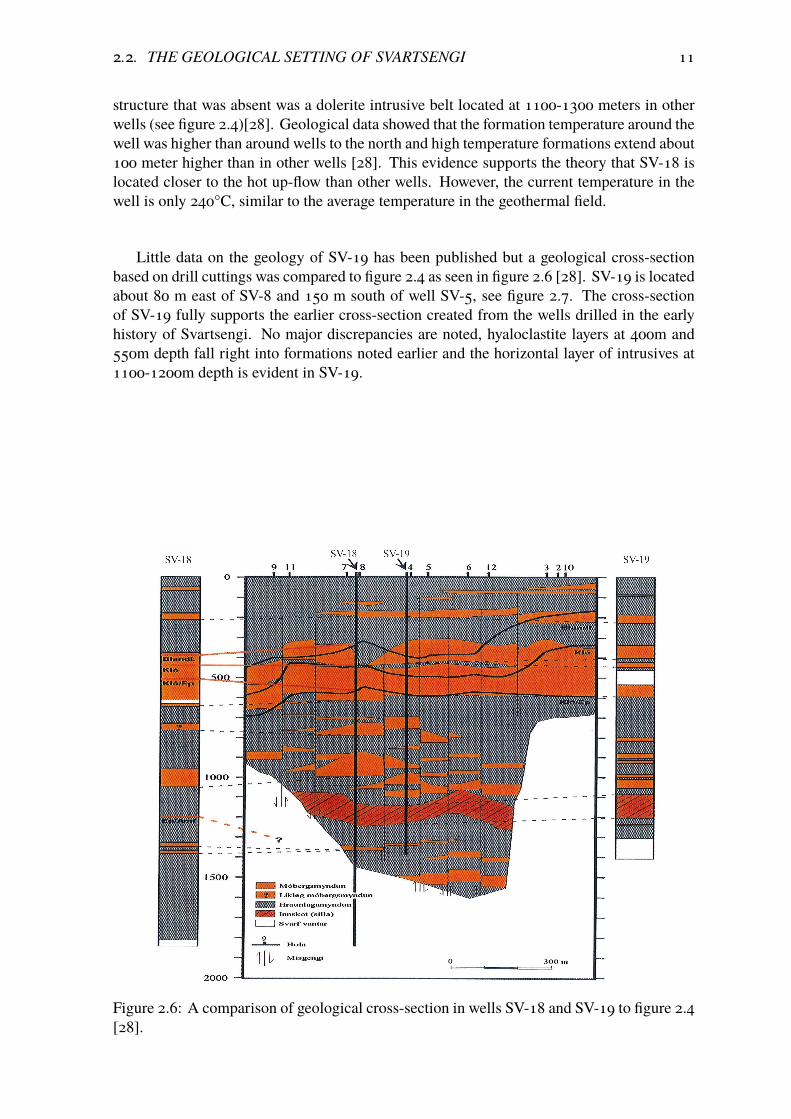
Little data on the geology of SV-19 has been published but a geological cross-sectionbased on drill cuttings was compared to figure 2.4 as seen in figure 2.6 [28]. SV-19 is locatedabout 80 m east of SV-8 and 150 m south of well SV-5, see figure 2.7. The cross-sectionof SV-19 fully supports the earlier cross-section created from the wells drilled in the earlyhistory of Svartsengi. No major discrepancies are noted, hyaloclastite layers at 400m and550m depth fall right into formations noted earlier and the horizontal layer of intrusives at1100-1200m depth is evident in SV-19.

Figure 2.6: A comparison of geological cross-section in wells SV-18 and SV-19 to figure 2.4[28].


Figure 2.7: Location of production wells at Svartsengi, direction of directionally drilledwells shown in red. Modified from [7].

SV-17 was drilled specifically as an injection well. The well is located 2.4 km WSWof the main production zone but resistivity measurements indicated that high temperaturescould be found at shallow depth in the area. The temperature of the well was measured to be240°C and capable of serving either as a production well or an injection well. Despite thedistance frommain production zone geological layers could be traced back to the same originof those of the production wells at Svartsengi, but the high temperature zone is believed to bepositioned 100-200 m lower than in other wells [29]. Feed points in the well are connectedwith two vertical basalt intrusions at a depth between 450-700 m, where a large number ofrelatively small feed points were noted. Horizontal fractures near the bottom of the wellcorrespond the two largest feed points in the well [29].

SV-24 was drilled within the same well platform as SV-17, like SV-17 it was intendedas an injection well right from the start. SV-24 is a directionally drilled well with a drilledlength of 1098 meters. Original plans had intended the well to be 2000 m deep but a highinjectivity index of 35 l/s/bar at 1000 m depth indicated a high permeability in the well andthere was no need to drill deeper. Main feed points in the well were noted at 649m and 674m[30].

The geologic cross-section in figure 2.4 and information from more recent boreholesshow a sequence of lava flows separated by hyaloclastite layers. The hyaloclastite layersare generally far less permeable than the lava layers, and therefore hinder the flow of fluid[19]. The thick layer of hyaloclastite at 300 to 600 meters depth is likely to act as a caprock,separating the geothermal reservoir from a shallow groundwater aquifer sitting on top. Thecaprock is fractured on the NE side of the reservoir, allowing up flow of geothermal fluid that


gives rise to the creation of a natural steam zone around wells SV-2, SV-3, SV-10, SV-14,SV-16 and SV-20 [26]. Local decrease in reservoir pressure due to production has causedthe natural steam zone to expand. The enlargement of the original steam zone caused wellsSV-7 and SV-11 to start producing both from the liquid dominated reservoir and the steamzone [31].

Later on in this study, when analysis of the tracer data is performed, parameters suchas distance between injection and production wells, depth of wells, casing depth, and feedpoints are used to evaluate tracer recovery and gain a further insight into the characteristics ofthe geothermal system. Detailed information about well and casing depths in the geothermalsystems at Svartsengi and Eldvörp were presented in [7]. Beneath the casing either a slottedliner or no liner has been inserted for the production portion of the wells and geothermalfluid can easily flow into the wells from various feed points. A summary of well feed pointswas created using available borehole logs and Franzson’s summary [26], [27], [28], [32],[33], [29], [30], [34]. Unfortunately, borehole logs or information about feed points was notavailable for all wells. Presented in table 2.1 is all data available from the sources mentionedabove. In addition, distances between wells were measured using Petrel [35], where distancesto and from directionally drilled wells were measured at the top of the wells. Note that thislist does not present all feed points encountered during drilling, but only those that wereconsidered likely to be large contributors to production from the wells. Note that, in general,the casing of steam zone wells is considerably shallower than those of two phase or liquidphase wells. The exception here is well SV-23, a steam phase only well, where the casingreaches down to 489 m. The reason behind that being that SV-23 is a directionally drilledwell; where the well head is located outside the original steam zone but drilled directionallyinto it.

The initial conceptual model proposed a trough shaped highly permeable 2 km2 reservoir,opposed to 6-8 km2 estimated by [23] and [22], with relatively impermeable boundaries onthree sides [24].This hypothesis has since been supported by numerous land subsidencemeasurements [36], [37]. The subsidence data presented in figure 2.8 provides a detailedsummary of data collected between 1967 and 1999. The data supports the original hypothesisand subsidence contours, extending from Svartsengi towards Eldvörp in the SW direction,showcase the hydrological connection between Svartsengi and Eldvörp. The short distancebetween contours east of Svartsengi show a rapid decline in subsidence rate, suggestinggeological formations that limit permeability in that direction [19]. Earthquake epicenterson the Reykjanes peninsula have been thoroughly studied through the years. The epicentersform a belt on the the peninsula that cuts through the Reykjanes geothermal field, Eldvörpand Svartsengi. Both Svartsegni and Eldvörp are located in the middle of the belt, as seenin figure 2.9. Earthquakes make way for cracks and fractures, consequently increasing thepermeability of the rock matrix. The outside boundaries of the earthquake belt are thereforelikely to form boundaries of lower permeability around the reservoir in the north and southdirection. This is supported by closeness of subsidence contours north and south of theSvartsengi. The land subsidence data not only gives an idea of the shape of the reservoir,it also provides information on the area geothermal fluid is being extracted from at depthand the relative lateral extent of the reservoir [19]. About 100 km2 of land area aroundSvartsengi has been affected by subsidence due to production, which is a much larger areathan the production zone itself [19],[37].


Table 2.1: Information about well depth and distances from reinjection wells.

Well Depth [m] Casing [m] Feed points [m] Distance from [m]

SV-24 SV-17

SV-7 1438 600 1350 2626 2598SV-8 1603.5 622 2640 2612SV-9 994 588 441, 907 2431 2401SV-10 425 220 3274 3244SV-11 1141 582 2436 2409SV-14 612.4 195 349-350 3230 3201SV-16 440 246 3316 3287SV-18 1845 770 735, 1815 2677 2651SV-19 1600 715 2776 2748SV-20 430.5 245 244-256,350, 404 3250 3221SV-21 1475 844 2354 2323SV-22 862 386 388, 410, 510-515, 620-640 3023 2994SV-23 698 489 608, 646 3096 3066EG-2 1265 520 2739 2761SV-17 1260 789 1052, 1125, 1220 — —SV-24 1086 300 649, 674 — —


Figure 2.8: Subsidence rate at the outer part of theReykjanes peninsula for four time intervals.Bench marks are shown by solid circles, roads are shown by thick lines, contour intervals are1 mm/year [37].

Figure 2.9: Location of main fussure swarms and earthquake belt on Reykjanes peninsula,modified from Kjaran et al., 1980 [19], [24].


2.3 The injection history of SvartstengiEarly on discussion started whether or not it would benefit the Svartsengi geothermal field toinject some of the production fluid into the field again. This came about after considerabledrawdown in the field was recorded in 1976 [2].In march 1982 the first injection well, SV-12, was drilled. It was drilled with the followingcriteria in mind [2]:

1. It was within the known reservoir.

2. It should have the potential to be used as a production well if injection was not feasible.

The well is located in the north end of the current production zone, about 200 m west ofSV-10. Before the injection test started it was proposed that brine would be injected for aweek into the reservoir, then hot fresh water for a week and then finally brine for 4-8 weeks.However, little was known about the effect of injecting brine into the reservoir, and at thetime changes were being made to the power plant so the supply of hot fresh water was limited.Thus the test was performed using cold water, which had the advantage of being in amplesupply but the disadvantages of larger temperature difference and higher risk of corrosion[38].

This first injection test lasted 24 days but during that time 63-65 l/s of cold water wereinjected into SV-12. The water level in SV-4 was monitored during the test along with thewater level in SV-12. The water level in SV-12 rose as soon as the tests started and abouta week after the injection stared a considerable increase was noted in SV-4. Along withthe increased water level there was an increase in the amount of gas in SV-4 which causedthe water level monitor to fail. About three weeks after injection had been terminated thewater level had fallen approximately 100 m. This first test showed that an injection intoSV-12 would provide a pressure support for the system and reduce drawdown. However, asimultaneous tracer test showed that the well might be located too close to the productionfield. The results from the tracer test will be discussed in further detail in a later section[38].

Following recommendations that were provided as a result of the injection test in 1982,another more extensive test was performed in 1984. Again the test was twofold, an injectiontest and simultaneous tracer tests. The supersaturation of the spent geothermal brine wasa cause for concern about silica deposits in the injection well and pipelines. One of thepurposes of this test was to see whether mixing condensate with the brine would allow thebrine to be injected without considerable silica deposits before reaching the reservoir. Thetest was done with a 20% condensate and 80% brine mixture at a flow rate of 50 l/s and lasted77 days. Again the water level in SV-4 showed a direct correlation to the amount that wasbeing injected into the system, or in other words the total amount of fluid extracted from thereservoir. However, the injection did not have a noticeable effect on other wells. The mixingof 20% condensate with the brine could not be maintained because at the second half of thetest the production of condensate dropped and only 10% mixing was achieved which did notturn out to be sufficient. A rapid increase in water level in SV-12 occurred and injection wasstopped to avoid permanently damaging the well.

Once the injection of condensate and brine mix had stopped the injection of hot freshwater into SV-12 was continued for about 4 years. During that time the flow rate ranged from40 kg/s to 90 kg/s. Once injection into well 12 was terminated, injection into SV-5 started and

2.3. THE INJECTION HISTORY OF SVARTSTENGI 17

continued for 2 years at a flow rate of 20-60 kg/s. The injection into well 5 was terminated in1990 and no more experiments were done with injection of fluid into the system for the nextthree years. In 1993 injection of condensate into SV-6 was started and done on and off forthe next 7 years. The injection from 1984-2000 was mostly of experimental nature and allthree wells, SV-12, SV-6 and SV-5 are located within the production zone. If injection hadbeen continued into these wells at the same flow rates, some pressure support would havebeen provided but a rapid cooling should have been expected in the field[1].

In 1998 the drilling of SV-17 was started. The well was intended to be an injection welland provide pressure support for the system without the risk of rapid cooling. The well is1260 km deep and located 2.5 km WSW of the production field. Injection into the well wasnot started until 2001 when 30 kg/s of condensate brine mixture was injected. In 1992 and1994 further research was done on the silica scaling problem experienced in 1984. There itwas determined that 38% of the mixture had to be condensate if only 1 mm of scaling wasallowed per year. If no scaling was permitted condensate had to account for 52%. Thus,the mixture injected into well SV-17 contains 40-50% condensate and 50-60% brine at atemperature of 95°C [1]. The injection was slowly increased from 30 kg/s in 2001 to 150kg/s in 2007 [39] [3].

In late 2008 SV-24 was added as a second injection well [4]. The well was drilled on thesame platform as SV-17, located about 2.3 km from the nearest production well. The injec-tion in well SV-24 started out slow, but in 2014 the total reinjection into the field averagedabout 300 kg/s, where approximately 35% of the fluid was injected in SV-24 [3]. In additionto the fluid injected by HS Orka, about 100 kg/s of cold ground water leaked into well SV-24from 2008 until the responsible feed point was sealed off in 2010 by HS Orka [7].

Temperature measurements done following the reinjection into SV-17 and SV-24 showthat temperature has not been affected by injection of the 95°C fluid. However, pressure datashow a good pressure support resulting from the injection in monitoring wells as illustratedin figure 2.10.

Figure 2.10: Pressure at 900 m depth in Svartsengi and Eldvörp from 1980-2013 [7].


The pressure data from Svartsengi and Eldvörp show a strong correlation between theoperation of the power plant and well pressure fluctuations. In November 1999 EnergyPlant V started producing electricity [40]. Shortly after, in 2000, the field pressure starteddropping at an increased rate. But in 2002, once injection into SV-17 had reached about55 kg/s, pressure started stabilizing and stayed almost constant until early 2008 [3],[7]. Inearly 2008 Energy Plant VI was commissioned and pressure started decreasing again [7].However, the new trend did not last; by the end of 2008 the pressure started increasing againdue to reinjection into SV-24. Since 2010 the pressure has been decreasing at a rate about1.1 bar/year due to the increased production intensity in 2008. The reason for the late arrivalof pressure decrease can likely be traced in some part back to the inflow of cold fluid intoSV-24 that was sealed off in 2010.

2.4 Tracer tests in the Svartsengi geothermal fieldAs previously stated, two combined injection and tracer tests were performed in the early1980s. The objectives and results of the injection tests were discussed in detail in the previoussection. The focus in this section will be on the purpose and results of the tracer tests.

The test performed in 1982 was the first tracer test in a high temperature field in Iceland,and due to lack of experience Hitaveita Sudurnesja decided to perform a simple test tobegin with[2]. Cold fresh water was injected into well SV-12. Sodium concentration in thegeothermal brine and nitrogen ratio in the gas coming from production wells were used astracers. The test was performed as described below [38]:

1. Cold fresh water at a flow rate of 63-65 l/s was injected into the newly drilled injectionwell, SV-12, for 24 days.

2. Brine samples were collected from the separators of wells 6-11 every 2 hours for 11weeks. Sampling was terminated after 70 days.

3. The concentration of sodium in the brine was analyzed. This was done to monitorthe salinity of the brine. If there was a short circuit between the injection well andany of the production wells, the salinity in that particular production well should dropsignificantly.

4. Steam phase and gas samples were taken everyweek after the first twoweeks tomonitorthe ratio of nitrogen in the gas. Carbon dioxide normally makes up about 98% of thegases that travel with the brine from the wells at Svartsengi. Fresh water containsoxygen and nitrogen and when the fresh water is injected into the reservoir those gasesare mixed in with the brine. The ratio of nitrogen in the gas of wells that are affectedby the in-flow of fresh water should rise compared to normal levels.Thus, the ratio ofnitrogen in the gas was used to gather information about how the injected fresh watertraveled through the reservoir.

Before the injection started brine samples were taken once per day for a week to get baseconcentration for each well. Wells SV-6, SV-9 and SV-10 all showed a change in sodiumconcentration, as seen in figure 2.11. Well SV-10 was the first to respond, 55 minutes af-ter injection started the sodium concentration in the well dropped from 7500 ppm to 4500ppm. After three hours the concentration had returned to normal. A drop in concentrationand a return to normal levels was observed two more times during the test period. Well

2.4. TRACER TESTS IN THE SVARTSENGI GEOTHERMAL FIELD 19

SV-9 showed a drop in sodium concentration of 6000 ppm 34 days after injection and 3days later the concentration had returned to normal values. Well 6 also showed a changein sodium concentration but the well had been shut in before the test and then again for 2hours during the test while the well was connected to the power plant. For the first weekof the test the well was discharged through a silencer. The changes in boiling and wellcondition thus made it hard to interpret the data. Wells SV-7, SV-8 and SV-11 did notshow a significant sodium concentration during the test. Similarly, wells 6 and SV-10 showsthe largest increase in nitrogen ratio in the gas samples. Wells SV-8, SV-9 and SV-11 doshow a response but considerably less than wells SV-6 and SV-10. as seen in figure 2.12 [38].

Figure 2.11: Sodium concentration in well SV-6, SV-9 and SV-10 [38].


Figure 2.12: Percentage of carbondioxide and nitrogen in gas in wells SV-6, SV-8, SV-9,SV-10 and SV-11 [38].

The main results from this first tracer test in a high temperature field in Iceland werethat well 12 was too close to the production field to be used as an injection well. The shortresponse time indicated that there was a very strong connection between well SV-10 andSV-12 and long term injection would most likely cause cooling in the field, and possibly veryrapidly. At this point further testing of the well was recommended [38].

In 1984 the second tracer test was performed at Svartsengi, based on guidelines from theprevious test. Again the test was performed in conjunctionwith an injection test inwell 12, theinjection test which was discussed in the previous section. This time two tracers were injectedinto the field, iodide and RhodamineWT. The tracers were chosen according to the guidelinesoutlined in background section about tracer tests. However, iodide did have a backgroundconcentration of 177 ppb [41]. The main purpose of using Rhodamine WT along with theiodide was to test its stability in a high temperature reservoir, the Rhodamine WT had beenused successfully in low temperature fields but had not been tested in high temperature fields.

On July 26th 37 liters of Rhodamine WT mixed with few a hundred liters of injectionfluid were injected into well SV-12. The day after 350 liters of potassium iodide dissolved ina few hundred liters of injection fluid were injected. The sampling frequency for this secondtest was much higher than of the first test to begin with. At first samples were collectedevery hour, but quickly decreased to 12, 6, 4 and then finally 2 samples per day. The firstsign of iodide occurred 40 hours after injection in well SV-6 and reached a peak value after100 hours [41]. It should be noted that well SV-10, the well that had shown the strongestconnection to well SV-12 in the previous test, was at this time producing solely from the

2.4. TRACER TESTS IN THE SVARTSENGI GEOTHERMAL FIELD 21

steam cap that had formed due to production, and no liquid samples could be obtained [2].Other wells that the iodide was detected in were wells SV-7 and SV-8. However, it wasestimated that only about 4% combined of the iodide injected was recovered in wells SV-7and SV-8 while 38% were recovered in well SV-6 [41]. The Rhodamine WT experiment didnot prove to be successful. The Rhodamine WT did show up in the system at the same timeas the iodide and reached a peak value after 100 hours. The concentration however is muchlower than would be expected based on the iodide return and drops off much faster. Thus,it was determined that the Rhodamine WT was not stable enough at such high temperaturesand silica deposits in the sample interfered with the analysis. The conclusions drawn fromthe tracer test were that:

1. Well SV-6 is fed through a single fracture and porous rocks. This was based on thefact that three models were needed to model the high peak and long tail of the recoverycurve [42].

2. Prolonged injection into well SV-12 would cause rapid cooling in well SV-6 and makeit unfit for production relatively quickly [41].

3. Wells south of the injection well would be most affected, but wells placed east andwest of well SV-12 would most likely not experience cooling until decades later [41].

The results from the 1982 and 1984 tracer tests were both in agreement that well SV-12 was too close to the production field to avoid cooling due to injection. The test alsoshowed that the predominant direction of flow in the field was consistent with the direc-tion of the fractures; north-south [41]. The wells south of the injection well had the highestand fastest recovery of tracers while wells west and east of well 12 had amuch lower recovery.

No other tracer tests have been performed in the Svartsengi field until now despitecontinuous injection into SV-17 and SV-24. The wells are located about 2.5 km south-westof the production zone. Thus, the current test is expected to take a considerably longer timethan the tests performed through SV-12 in the 1980s.

23

Chapter 3

Methods

The tracer test at Svartsengi began on June 23rd 2015 when 400 kg of the liquid phasetracer 2,6-napthalene disulfonate (NDS) were dissolved in 12 m3 of water, and injected intowell SV-24. The injection lasted about 20 minutes. Liquid background samples were takenon June 19th and at the end of May by Iceland GeoSurvey (ÍSOR). The first samples aftertracer injection were taken on June 25th. On June 28th 86,78 kg of the steam phase tracersulfurhexafluoride (SF6) were injected into well SV-24. The tracer injection took 11 hoursand 39 minutes. Background steam samples were taken by ÍSOR at the end of May and thefirst samples after injection of tracer were taken June 30th and July 1st. On July 8th 400 kgof the liquid phase tracer 2,7-NDS dissolved in approximately 12 m3 of water were injectedinto well SV-17. The injection lasted 30 minutes.

The sampling schedule was designed according to general rules described in section 2.1.Both steam and liquid phase sampling schedules are presented in table 3.1

Table 3.1: Sampling schedule for both SF6 and NDS.

Liquid phase Steam Phase

Week Sampling Frequency Week Sampling Frequency

1 1x per week 1-2 3x per week2-6 3x per week 3-8 2x per week7-9 2x per week 9-14 1x per week10> 1x per week 15-17 Every other week

The distance between the injection wells and the closest production well is about 2.3 km,see table 2.1. Thus, the chance of the liquid tracer showing up in the system within the firstweek were determined to be extremely low and only one sample was taken in the first week.The following five weeks the sampling frequency was increased to three times per week incase the liquid tracer traveled with high velocity through the system and a sharp peak wouldbe experienced. After seven weeks without any signs of the liquid tracers it was determinedthat the chances of a sharp peak would be highly unlikely and the it was safe to reduce thesampling frequency without running the risk of losing any significant data. At this point thesampling frequency for the liquid phase was reduced down to twice per week and two weekslater down to once per week.

24 CHAPTER 3. METHODS

The steam tracer was expected to travel at a much greater speed through the system dueto a much lower density and higher entropy of the gas phase than the liquid phase. Therefore,the sampling frequency for the steam phase tracers started out at three times per week tomake sure all sharp peaks would be detected. Two weeks after injection the frequency wasreduced down to twice a week. At this point it was determined that the SF6 traveled at alow enough speed through the system that no important information would be lost with areduced frequency. The steam tracer was first detected 18 days past injection in wells SV-7and SV-11. On August 20th it was determined to reduce the sampling frequency down toonce per week in the following week, week 9. At this point the concentration of SF6 hadalready reached a maximum and the concentrations for each well were coming down at asteady pace close to detection limits. However, the next batch of results showed that theconcentration was starting to rise again in a couple of the wells. This posed the questionwhether the frequency should be increased again or kept at the current rate. It was determinedthat given the previous pattern of tracer returns and the relatively long time past injectionthat a sharp peak would not be very likely and one sample per week would be sufficient.The sampling frequency of one sample per week was kept constant through September. Atthe end of September the concentration had dropped down to detection limits. At this pointit was considered highly unlikely that the concentration would rise again and the samplingfrequency was reduced down to every other week until steam sampling was terminated inweek 17.

3.1 Sampling methods

3.1.1 Vapor phase sampling methodsA Giggenbach glass bottle was used for gas phase samples. 52 bottles were used for thisexperiment, each bottle was weighed when empty and then filled with water to calculateexact volume. Due to the number of monitoring wells and sampling frequency there wasa rather quick turn around for each bottle for the first few weeks. Each bottle was cleanedthoroughly before 100 ml of 10 M NaOH solution was added to the bottle. Finally, the bottlewas evacuated for 4 minutes and weighed.

The gas phase at Svartsengi consists mainly of CO2 and H2S. In fact CO2 and H2S makeup about 99 mole% of the gas coming from the wells [43]. Thus, the caustic solution is addedto Giggenbach bottle before sampling, acidic gases dissolve in the NaOH solution allowingthe other gases to be collected in the headspace in detectable concentrations.

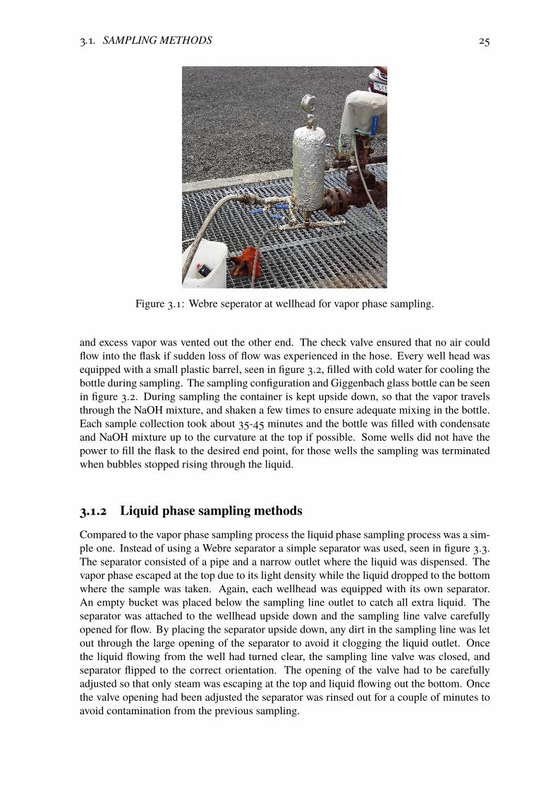
A Webre separator, shown in figure 3.1, was utilized at the wellhead. Each well had itsown Webre separator to minimize contamination between wells.

At the start of sampling geothermal fluid from the well was allowed to flow through bothvapor and fluid vent with a full opening to rinse out separator from last sampling. Once theseparator had been rinsed out for a couple of minutes the vapor vent was adjusted so that ablue cone formed at the outlet. The blue cone is an indicator that dry steam is being vented[44]. The water vent was kept at a full opening throughout the sampling process, allowingwater level in the separator to remain low to ensure the best quality of the vapor sample.After adjusting the vapor outlet, a silicone hose was attached and rinsed for a couple ofminutes before it was attached to the Giggenbach bottle. The silicone hose was fitted with ay-connection and a check valve. The end without the check valve was connected to the bottle

3.1. SAMPLING METHODS 25

Figure 3.1: Webre seperator at wellhead for vapor phase sampling.

and excess vapor was vented out the other end. The check valve ensured that no air couldflow into the flask if sudden loss of flow was experienced in the hose. Every well head wasequipped with a small plastic barrel, seen in figure 3.2, filled with cold water for cooling thebottle during sampling. The sampling configuration and Giggenbach glass bottle can be seenin figure 3.2. During sampling the container is kept upside down, so that the vapor travelsthrough the NaOH mixture, and shaken a few times to ensure adequate mixing in the bottle.Each sample collection took about 35-45 minutes and the bottle was filled with condensateand NaOH mixture up to the curvature at the top if possible. Some wells did not have thepower to fill the flask to the desired end point, for those wells the sampling was terminatedwhen bubbles stopped rising through the liquid.

3.1.2 Liquid phase sampling methods

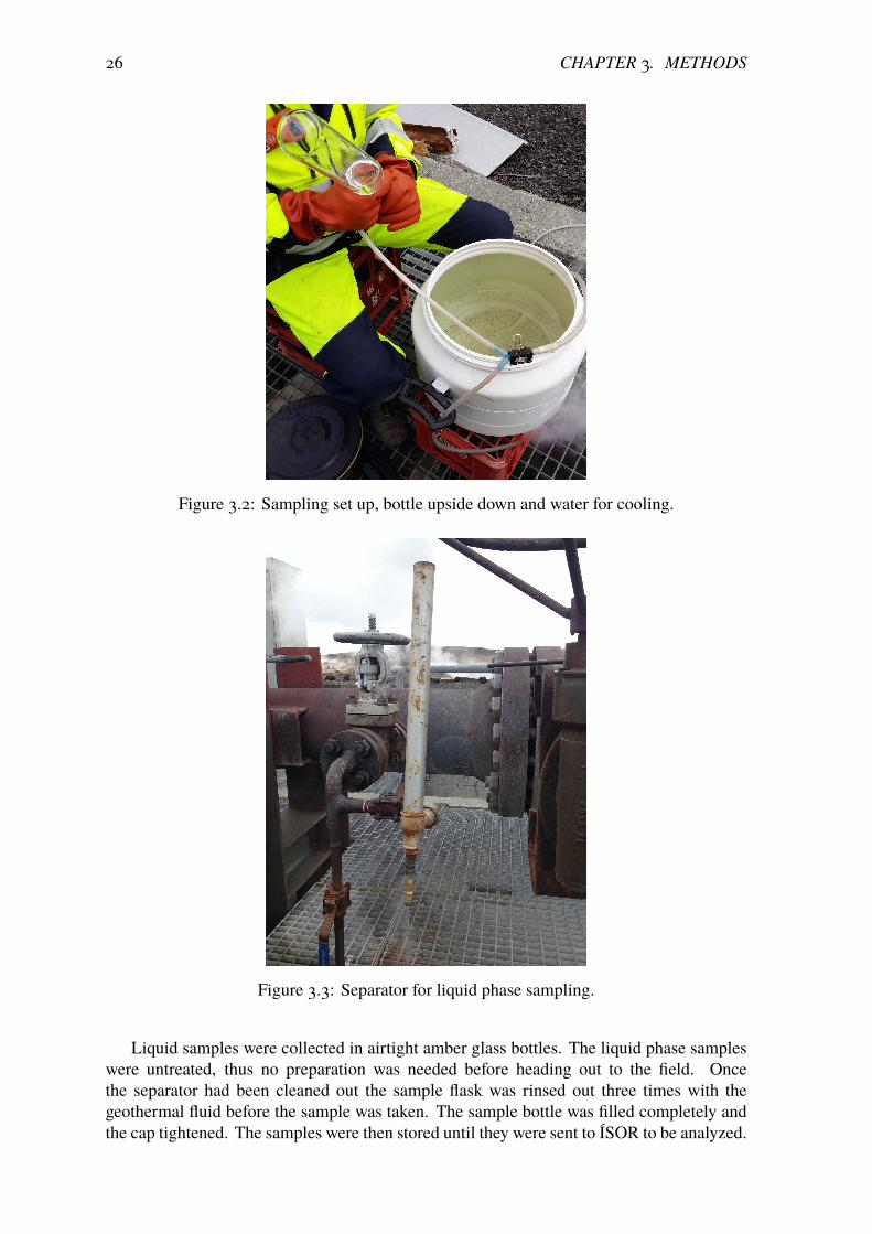
Compared to the vapor phase sampling process the liquid phase sampling process was a sim-ple one. Instead of using a Webre separator a simple separator was used, seen in figure 3.3.The separator consisted of a pipe and a narrow outlet where the liquid was dispensed. Thevapor phase escaped at the top due to its light density while the liquid dropped to the bottomwhere the sample was taken. Again, each wellhead was equipped with its own separator.An empty bucket was placed below the sampling line outlet to catch all extra liquid. Theseparator was attached to the wellhead upside down and the sampling line valve carefullyopened for flow. By placing the separator upside down, any dirt in the sampling line was letout through the large opening of the separator to avoid it clogging the liquid outlet. Oncethe liquid flowing from the well had turned clear, the sampling line valve was closed, andseparator flipped to the correct orientation. The opening of the valve had to be carefullyadjusted so that only steam was escaping at the top and liquid flowing out the bottom. Oncethe valve opening had been adjusted the separator was rinsed out for a couple of minutes toavoid contamination from the previous sampling.


Figure 3.2: Sampling set up, bottle upside down and water for cooling.

Figure 3.3: Separator for liquid phase sampling.

Liquid samples were collected in airtight amber glass bottles. The liquid phase sampleswere untreated, thus no preparation was needed before heading out to the field. Oncethe separator had been cleaned out the sample flask was rinsed out three times with thegeothermal fluid before the sample was taken. The sample bottle was filled completely andthe cap tightened. The samples were then stored until they were sent to ÍSOR to be analyzed.

3.2. ANALYTICAL METHODS 27

3.2 Analytical methods

All samples were analyzed by ÍSOR using their equipment and techniques. The followingtwo sections will describe in detail what methods were used to analyze the samples andcalculate SF6, 2,7-NDS and 2,6-NDS concentrations.

3.2.1 Vapor phase sample analytical methods

The SF6 samples were analyzed using a Thermo Scientific Trace 1310 gas chromatographequipped with a TG Bond Alumnia Na2SO4 analytical column and an electron capture detec-tor (ECD). 99.999% pure nitrogen was used as both make-up and carrier gas. The preferredsoftware for instrumental control and data analysis was Chromeleon, version 7.2. The injec-tion and oven temperatures were kept at 373 kelvin and 333 kelvin respectively. Injectiontime for each sample was 1 minute and run-time was kept at 7 minutes.

The method used to calculate the concentration of SF6 in the samples is based on thesame principle as many chemical analytical methods. The detector in the gas chromatographyields a spectra with a peak for the analyte. Thus, the first step was to run the samples fromthe field through the gas chromatograph and achieve a spectra for each sample. The secondstep was to create a standard curve by running a series of samples with a known concentrationof SF6 through the gas chromatograph. The standard curve correlates the area of the peak tonumber of moles of SF6 in the samples from the field. Using the ideal gas law the numberof moles in the injection line can be calculated:

nline =PlineVline

RT(3.1)

Where nline is the total number of moles in the injection line, Pline is the pressure of thesample in the injection line in millibar, Vline is the volume of the injection line in milliliters,R is the gas constant in milliliter-millibar/kelvin-mol and T is the temperature of the samplein kelvin. Here the volume of the injection line was 28.68 mL.

When the standard curve is created the standard gas is injected at different pressures tovary the number of moles in the injection line. Since the concentration of SF6 in the standardis known, in this case 1 ppm, the total number of moles SF6 in the known volume of thesampling line can be calculated:

nlineSF6 = 1x10−6nline (3.2)

Once enough data points have been obtained to create a standard curve with peak areasof the same scale as those of the unknown samples, analysis of the unknown samples canbegin. The standard curve used in this particular case is presented in figure 3.4.


Figure 3.4: Standard curve that correlates peak areas to number of moles in injection line,data provided by ÍSOR.

Using the standard curve, the number of moles in the sampling line for the unknownconcentration can now be calculated. Once nlineSF6 is known, the volume of the headspacein the sample is calculated. Before each flask was used, it was weighed before the additionof NaOH and after evacuation as described in section 3.1.1. After sampling, the flask wasweighed again and the weight recorded. This information was used to calculate the volumeof the headspace in the flask using equation 3.3:

Vhs = Vf −(m f ull − mempty)

ρNaOH(3.3)

Where Vhs is the volume of the headspace in milliliters, Vf is the volume of the samplingflask, ρNaOH is the density of the NaOH solution in g/mL, m f ull is the mass of the flask aftersampling in grams, mempty is the mass of the empty flask in grams.During each run the temperature and pressure of the injection line and the sample flask areequal. Thus, Avogadros’s law can be applied to calculate the number of moles in the sample:

nSF6 = nlineSF6

Vtotal

Vline(3.4)

Where Vtotal is given by:Vtotal = Vhs + Vline (3.5)

Once the number of SF6 moles in the sample have been calculated, the mass of SF6 inthe sample is calculated using the molar mass of SF6:

mSF6 = M (SF6)nSF6 (3.6)

Where mSF6 is the mass of SF6 in grams, and M (SF6) is the molar mass of SF6, which isequal to 146.06 g/mol. Finally, the mass fraction of SF6 in the sample is calculated. Here

3.3. MODELING METHODS 29

the first step is to calculate the total sample mass:

msample = (m f ull − mevacuated)kg

1000g(3.7)

where msample is the mass of the sample in kg, m f ull is the mass of the flask after sampling ingrams and mevacuated is the mass of the flask after evacuation. Once the mass of the sampleitself is known the mass fraction in the sample can be calculated:

c =mSF6

msample(3.8)

where c is the mass fraction in g/kgcondensate.

The limiting factor for the method was high concentration of standard gas availablecompared to the peak areas of the unknown samples. The samples with a concentrationbelow approximately 0.02 ppb (or 2x10−5 mg/kg condensate) could not be analyzed with ahigh degree of certainty. The reason for this is that those concentrations fall below the scopeof the available standard curve, and due to non-linearity of the data, extrapolation can not beguaranteed.

3.2.2 Liquid phase analytical methodsThe liquid phase samples were analyzed in a high performance liquid chromatograph (HPLC)using fluorescence spectroscopy at the ÍSOR lab. The HPLC solution used was a UlitMate3000 from Dionex, equipped with a 50 mm x 2.1 mm BetaBasic column from Dionex anda fluorescent detector [45]. The detector’s excitation wavelength was set at 225 nm andemission wavelength was set at 340 nm. Injector volume for the HPLC was 20 µg and flowrate between 0.5-0.7 mL/min. The system pressure was 170-190 bar. The mobile phaseconsisted of phosphate buffer in methanol/water mixture. The phosphate buffer consistedof 3.17 mM Na2HPO4, 6.21 mM KH2PO4 and 5.0 mM (CH3CH2CH2CH2)4N[OP(OH)2O](TBAP). The methanol/water mixture consisted of 25% methanol and 75% water. ThisHPLC method resulted in chromatographic separation of 2,6 NDS and 2,7 NDS from eachother and from reservoir interferences [46]. The runtime for each sample was 15 min.

To clean the samples before each run theywere filtered using a 0.22 µmnylon filter. Beforeeach run 5 standards mixed with geothermal brine from SV-7 were run through the UltiMate3000. Those standards were 0.1 ppb, 0.5 ppb, 1 ppb, 5 ppb and 10 ppb. Additionally, the 5standards were run through the system after every 10th sample. The detection limit of 2,6NDS and 2,7 NDS in the HPLC was 0.2 ppb.

3.3 Modeling methodsThe main goal with this paper is to increase the understanding of the characteristics ofthe Svartsengi geothermal system and estimate the risk of a cold front due to the currentreinjection into the field. In order to do that the tracer returns were modeled quantitativelyusing a couple of programs included in the ICEBOX software package. The programs thatwere used were TRINV, for simulating tracer returns, and TRCOOL, for creating long termcooling predictions in production wells.


3.3.1 Tracer transportThe TRINV software was developed by Orkustofnun and has been used successfully innumerous geothermal fields around the world [47], [48], [10]. The software is based onprinciples of the theory of solute transport, which was discussed in detail in section 2.1, andon the basis of one dimensional flow-channel model [10]. In reality wells are connectedby complex nets of fracture-zones, interbeds and layers, the one dimensional flow channelmodel, however, assumes that the flow between an injection well and a production well canbe modeled by one or more flow channels. These one dimensional flow channels are used todescribe the parts of these structures that are relevant to each pair of injection and productionwells. Since the model assumes flow only in one direction, the differential equation for tracertransport equation 2.5 can be simplified to [10]:

D∂2C∂x2 = u

∂C∂x+∂C∂t

(3.9)

Where D is the dispersion coefficient in m2/s given by equation 3.10, C is the tracerconcentration in the channel in kg/m3 at a distance x, x is the distance along the flow channelin meters, and u is the average fluid velocity given in m/s, described by equation 3.11. Inthe model mechanical dispersion is assumed to dominate molecular dispersion, thus thedispersion coefficient is given by:

D = αLu (3.10)

Where αL is the longitudinal dispersivity of the channel in meters and u is average fluidvelocity given by:

u =qρAφ

(3.11)

Where q is the injection flow rate in the flow channel in kg/s, ρ is the geothermal fluid densityin kg/m3, A is the average cross-sectional area of the flow channel in m2 and φ is the porosityof the channel.

If some amount of tracer , M , is assumed to be injected instantaneously and moleculardiffusion is ignored, tracer concentration in the production well is given by [10],[47], [49]:

c(t) =uMr ρ

Q1

2√πDt

e(−(x−ut)2/4Dt) (3.12)

Where Mr is the tracer mass flowing along the channel in kg, Q is the production rate in kg/sand x is the distance between the injection well and production well in meters.

The conservation of mass law correlates the tracer concentration in the production well tothe tracer concentration in the fracture zone, and is the basis for simulating the tracer returndata with equation 3.12 [50],[10]:

c(t)Q = C(t)q (3.13)

Where c(t) is the concentration of tracer in the production well fluid in kg/m3, Q is theproduction rate in kg/s, C(t) is the concentration of tracer in the flow channel and q is theinjection flow rate in the flow channel in kg/s.


In cases where the production well and injection well are connected by more than oneflow channel equation 3.12 becomes [47], [49]:

c(t) =n∑

i=1

ui Mr,i ρ

Q1

2√πDit

e(−(xi−ui t)2/4Di t) (3.14)

where c(t) is the concentration of tracer in the produced fluid, n is the number of flowchannels Mr,i is the tracer mass in flow channel i and xi the distance along flow-path i. ui,qi and Di are the average linear velocity along flow-path i, flow rate in channel i and thedispersion coefficient in flow-channel i, respectively, given by:

ui =qi

ρAiφi(3.15)

Di = αLiui (3.16)

qi =Mr,i

Mqin j (3.17)

where Ai is the cross-sectional area of flow-path i, φi is the porosity of channel i, αLi is thelongitudinal dispersivity of flow-channel i and qi is the flow of geothermal fluid in flow-pathi, and qin j is the injection rate.

The name of the software,TRINV, stands for tracer inversion. The flow channel propertiesare the flow channel cross-sectional area (Aiφi), the flow channel dispersivity (αLi) and theflow channel length (x). During the modeling the flow channel length is fixed as the distancebetween the main feed-zones of the two wells involved. As the name indicates, the softwaresolves equations 3.14-3.17 inversely using a non-linear least squares fitting to simulate thetracer return data and obtain the model parameters [10], [47]. The one-dimensional flowchannel model does not yield a unique solution to the problem, especially when consideringmultiple flow channels. Thus, a thorough understanding of the system and the tracer testdata is required when analyzing the solutions and estimating the most likely solution to theproblem [47].

Once the most probable solution has been determined, TRCOOL is used to make coolingpredictions. The TRINV program gave information about the flow channels in the system.This information is part of the input into the TRCOOL program. Temperature changes dueto long term reinjection are dependent on the properties of the flow channels, not only theirvolume but mainly on porosity and surface area [10]. Thus, in order to get the most accuratepredictions of the temperature decline, those parameters need to be estimated by looking atgeological and geophysical data from the field.

3.3.2 Thermal breakthroughThe reservoir rockmatrix acts as a heat exchangerwhenwater colder than reservoir conditionsis injected into the system. The capacity of the heat exchanger depends on the contact surfacearea between the rock and the fluid, the heat capacity of both the rock and the geothermalfluid, and the thermal conductivity of the rock. Thermal breakthrough can be predicted usinga similar equation to the one describing advancement of tracers. The thermal changes canbe described using equation 3.18 [51]:

Rthermal∂T∂t+ u · ∇T = κ∇2T (3.18)


where κ is the thermal diffusivity in m2/s and Rthermal is the unitless thermal retardationcoefficient. κ and Rthermal are further defined by

Rthermal = 1 +(1 − φ)ρRcR

φρwcw(3.19)

andκ =

kth

φρRcR(3.20)

where ρR is the density of the rock in kg/m3, cR is the specific heat capacity of the rockin J/Kg/°C, φ is the unit-less porosity of the rock matrix and kth is the thermal conductivityof the formation in W/m/°C.

Studies on the propagation of a thermal front in single phase, porous medium have shownthat due to the thermal inertia of the rock volume, the thermal front lags behind the fluid frontby a constant factor related to the volumetric heat capacity [51],[52],[53]. In other words,in homogeneous media, free of diffusive and dispersive effects, a sharp transition from thereservoir temperature to injection temperature should be expected behind the injection front.The mixing of geothermal and injection fluid, however, is largely controlled by diffusive ordispersive effects that cause both an earlier and more gradual decrease in the productiontemperature.

If we imagine a simple conceptual model shown in figure 3.5 describing transport alonga fissure then the thermal transport can be described by [54]:

Rthermal∂T f

∂t+ u

∂T f

∂x− D

∂2T f

∂x2 −κ′mb∂Tm

∂y

��y=b

= 0, |y | ≤ b (3.21)

and∂Tm

∂t= κm

∂2Tm

∂x2 , |y | > b (3.22)

.where T f is the temperature withing the fracture zone matrix and Tm is the temperature

in the rock matrix. Here κm is the thermal diffusivity in the rock matrix outside the fracture,further defined as

κm =kth

φρmcm(3.23)

where ρm is the density of the rock matrix outside the fracture and cm is the specific heatcapacity of the rock matrix outside the fracture.

κ′m is the thermal diffusivity within the fracture zone matrix, similarly defined as

κ′m =kth

φρ f c f(3.24)

where the subscript f denotes properties of the fracture zone material. Note that the fractureis not completely free of rock and open to flow of pure geothermal fluid.


Figure 3.5: Diagram of an idealized single fracture matrix system [54].

In the model presented here, the mechanical dispersion term from the tracer modelabove has been retained. However, in a solution presented by Carslaw and Jaeger [55] thedispersion is assumed to have an insignificant effect on thermal breakthrough. For steadyflow conditions the production temperature, TP(L, t) becomes:

TP(L, t) = T0 − ωin jqQ

(T0 − TI ) erfc[

kthL/(φρwcw)2bu√κm(t − Rthermal x/u)

h(

utRthermal

− x)]

(3.25)

Where T0 is the initial formation temperature in °C, ωin j is the fraction of injected fluidreaching the production well, which is equal to the ratio Mi/M , TI is the temperature ofinjected fluid in °C, L is the length of the flow channel in meters, b is half the width ofthe fracture-zone in meters, and h is the height of the flow-path inside the fracture-zone inmeters. Note that for multiple flow channels the solution is:

TP(L, t) = T0 −n∑

i=1ωin j,i

qi

Q(T0 −TI ) erfc

[kthLi/(φi ρwcw)

2biui√κm,i (t − Rthermal,i xi/ui)

hi

(uit

Rthermal,i− xi

)]

(3.26)The equations presented above (eq. 3.25 and 3.26) are valid at times t > Rthermal x

u .

The solution presented here above is the one used by TRCOOL to predict thermal break-through in production wells based on tracer test data. Several parameters control the arrivalof thermal changes, including the thermal retardation factor, the fracture opening, the poros-ity of the channel and the matrix diffusivity. However, the fraction of injected fluid reachingthe well, the production rate and the temperate difference between the reservoir and injectedfluid sets the limit for the magnitude of cooling. In this solution dispersion is assumed tohave an insignificant affect on the thermal breakthrough. However, it should be noted that inreality dispersion does in fact play a role in the process. By including the dispersive part inthe solution it is possible that an improved prediction would be achieved.


The results of the tracer test is used to estimate the average linear velocity in the fracture(u) and the cross-sectional area (Aφ). From there assumptions are often made about thesurface area available for heat transfer. It is recommended that this be done for at least twoextremes. One where the surface area is small, or a pipe like flow channel, this would resultin the most rapid cooling prediction. The other scenario would be a larger surface area flowchannel, similar to a thin horizontal layer, that is amore optimistic scenario resulting in slowercooling. Reasonable estimates of the formation density, heat capacity, and thermal conduc-tivity can either be found by using likely values from the literature or measuring samplesfrom the formation. In this case the likely values from the literature will be used due to thelong research and production history of Svartsengi. An estimate of the fracture porosity canoften be found in the literature, but if no such value is available a conservative value should beused in order to avoid underestimating the onset of thermal breakthrough [54]. The fractureporosity, along with the fracture aperture and unforeseen changes in the flow field due toproduction are the most uncertain parameters affecting the thermal breakthrough predictions.

When thermal breakthrough predictions are made based on tracer tests the underlyingassumption is that the fluid and temperature fronts follow the same paths from injection toextraction wells. One must keep in mind that over the course of long term production of ageothermal field this assumption may not be valid [54]. Chemical changes in the reservoirfluid, pressure drawdown and thermal changes due to production can alter flow-paths in thereservoir. Decreased reservoir temperatures within the field can lead to increased viscosityof the reservoir fluid and consequently slow down the thermal breakthrough [56]. However,significant changes to viscosity are more pronounced in cases where the temperature changesare very drastic. Thus, this phenomenon is unlikely to have a considerable effect on thethermal breakthrough predictions. Another factor that might alter flow paths in the reservoirare varying flow rates, such as injection and production rates. During geothermal utilizationthe injection and production rates are bound to vary to some extend and that was indeed thecase over the duration of this tracer test, as will be illustrated further in section 4.1. Themodel however is not designed to account for large variations on production or injectionrates, thus average rates were used for the analysis of the data.

35

Chapter 4

Results

4.1 Tracer recoveryIn this section the tracer recovery in different wells will pe presented. The amount of recov-ered tracer will also be calculated and the concentration of tracer in production wells will bediscussed.

Before the data can be analyzed in any way the tracer recovery must be estimated for eachproduction well of the test. The amount of tracer throughout the test was estimated based onequation 4.1:

mi (t) =∫ t

0ci (s)Qi (s)ds (4.1)

where mi (t) is the cumulative mass recovered in production well i in kg at time t, ci is thetracer concentration in the production well in kg/L or kg/kg and Qi is the production rate ofthe well i in L/s or kg/s.

At the time of writing liquid tracer has only been detected in small concentrations intwo samples, both from SV-9, thus minimum discussion will be on the results of the liquidtracer test as it is still ongoing. 2,6-NDS was detected in both samples, but no 2,7-NDS wasdetected. Preliminary observations indicate that the injected fluid from SV-24 does arrive inthe production wells slightly quicker than fluid injected into well SV-17.

The first step in determining the tracer return was to gather information about the pro-duction from each well over the duration of the test. Due to annual maintenance stops thatoverlapped with the test, variation in production rates were rather large, as seen in figure 4.1.Wells SV-10, SV-16, SV-20 and SV-23 produce purely from the steam zone while SV-22,SV-11 and SV-7 are wet steam wells. In order to calculate the portion of steam in the wetsteam wells a couple of different methods were used. According to HS ORKA (personalcommunication with Ómar Sigurðsson), the enthalpy of well SV-22 is around 1850 kJ/kg.Using the enthalpy of the well and steam tables the quality of the steam was determinedusing the following equation:

xv =hgeo f − h f

hg − h f(4.2)

where xv is the vapor quality, hgeo f is the enthalpy of geothermal fluid in the well (1850kJ/kg), h f is the enthalpy of saturated liquid state and hg is the enthalpy of saturated vapor

36 CHAPTER 4. RESULTS

state. At the separator pressure of 5.5 bar the value of h f and hg are 655.4 kJ/kg and 2752.8kJ/kg, respectively [57]. According to equation 4.2 the vapor fraction in well SV-22 is 0.57,which is in agreement with a value obtained by Þorvaldsson et al. [3]. For wells SV-7 andSV-11 values published by [3] were used, considering how recent the data was and howwell calculations for SV-22 matched up to it. It was determined that these numbers werean accurate description of the current status of those two wells. Both wells produce about22.4% steam and 81.6% fluid at the separator pressure. Using these fractions new productionnumbers for steam only were calculated and presented in figure 4.2.

Figure 4.1: Production variations throughout the steam phase test

One of the objectives of this thesis was to determine whether the appropriate amountof tracer was injected. For best results the concentration of tracer in the production wellsshould reach at least 5-10 times the detection limit, at the peak concentration in the well.The lowest area for the 1 ppm standard is 0.32 kHz/min, which yields a concentration around2x10−8 g/kgcondensate, or 0.02 ppb [8]. Despite the detection limit of the equipment beinglower than 0.02 ppb, samples with concentrations below 0.02 ppb could not be analyzedwith a high degree of accuracy. Thus 0.02 ppb is taken as the reference point here. Ap-proximately 60% of the samples, where SF6 was detected, yielded a spectra with a peakarea below 0.32 kHz/min. In order to create a standard curve for samples with such a lowconcentration using a 1 ppm standard the gas had to be put under a pressure down to 10mbar, in other words, down to the lowest pressure the equipment capable of. This createda higher risk of error incorporated into the standard curve. According to test that were per-formed at ÍSOR to evaluate the standard curve the deviation was in the range of -5.3% - 7.2%.

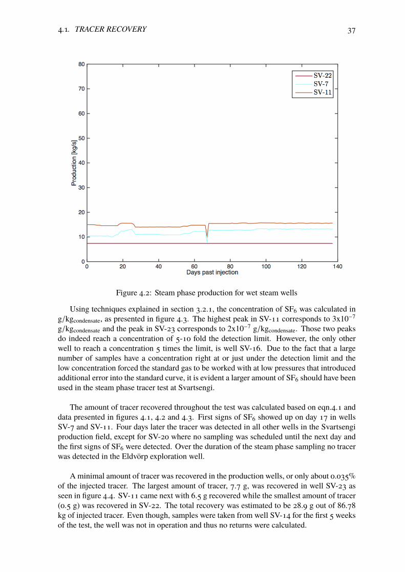
4.1. TRACER RECOVERY 37

Figure 4.2: Steam phase production for wet steam wells

Using techniques explained in section 3.2.1, the concentration of SF6 was calculated ing/kgcondensate, as presented in figure 4.3. The highest peak in SV-11 corresponds to 3x10−7

g/kgcondensate and the peak in SV-23 corresponds to 2x10−7 g/kgcondensate. Those two peaksdo indeed reach a concentration of 5-10 fold the detection limit. However, the only otherwell to reach a concentration 5 times the limit, is well SV-16. Due to the fact that a largenumber of samples have a concentration right at or just under the detection limit and thelow concentration forced the standard gas to be worked with at low pressures that introducedadditional error into the standard curve, it is evident a larger amount of SF6 should have beenused in the steam phase tracer test at Svartsengi.

The amount of tracer recovered throughout the test was calculated based on eqn.4.1 anddata presented in figures 4.1, 4.2 and 4.3. First signs of SF6 showed up on day 17 in wellsSV-7 and SV-11. Four days later the tracer was detected in all other wells in the Svartsengiproduction field, except for SV-20 where no sampling was scheduled until the next day andthe first signs of SF6 were detected. Over the duration of the steam phase sampling no tracerwas detected in the Eldvörp exploration well.

A minimal amount of tracer was recovered in the production wells, or only about 0.035%of the injected tracer. The largest amount of tracer, 7.7 g, was recovered in well SV-23 asseen in figure 4.4. SV-11 came next with 6.5 g recovered while the smallest amount of tracer(0.5 g) was recovered in SV-22. The total recovery was estimated to be 28.9 g out of 86.78kg of injected tracer. Even though, samples were taken from well SV-14 for the first 5 weeksof the test, the well was not in operation and thus no returns were calculated.


Figure 4.3: Concentration of SF6 in production wells

Figure 4.4: Cumulative SF6 returns per well

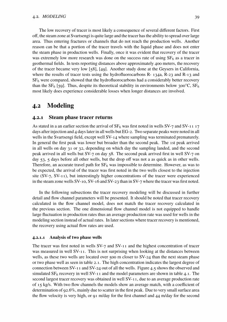
4.2. MODELING 39

The low recovery of tracer is most likely a consequence of several different factors. Firstoff, the steam zone at Svartsengi is quite large and the tracer has the ability to spread over largearea. Thus entering fractures or channels that do not reach the production wells. Anotherreason can be that a portion of the tracer travels with the liquid phase and does not enterthe steam phase in production wells. Finally, once it was evident that recovery of the tracerwas extremely low more research was done on the success rate of using SF6 as a tracer ingeothermal fields. In tests reporting distances above approximately 400 meters, the recoveryof the tracer became very low [58], [49]. Another study done at the Geysers in California,where the results of tracer tests using the hydrofluorocarbons R- 134a, R-23 and R-13 andSF6 were compared, showed that the hydrofluorocarbons had a considerably better recoverythan the SF6 [59]. Thus, despite its theoretical stability in environments below 300°C, SF6most likely does experience considerable losses when longer distances are involved.

4.2 Modeling

4.2.1 Steam phase tracer returnsAs stated in a an earlier section the arrival of SF6 was first noted in wells SV-7 and SV-11 17days after injection and 4 days later in all wells but EG-2. Two separate peakswere noted in allwells in the Svartsengi field, except well SV-14 where sampling was terminated prematurely.In general the first peak was lower but broader than the second peak. The 1st peak arrivedin all wells on day 31 or 32, depending on which day the sampling landed, and the secondpeak arrived in all wells but SV-7 on day 58. The second peak arrived first in well SV-7 onday 53, 5 days before all other wells, but the drop off was not a as quick as in other wells.Therefore, an accurate travel path for SF6 was impossible to determine. However, as was tobe expected, the arrival of the tracer was first noted in the two wells closest to the injectionsite (SV-7, SV-11), but interestingly higher concentrations of the tracer were experiencedin the steam zonewells SV-10, SV-16 and SV-23 than in SV-7where the tracer was first noted.

In the following subsections the tracer recovery modeling will be discussed in furtherdetail and flow channel parameters will be presented. It should be noted that tracer recoverycalculated in the flow channel model, does not match the tracer recovery calculated inthe previous section. The one dimensional flow channel model is not equipped to handlelarge fluctuation in production rates thus an average production rate was used for wells in themodeling section instead of actual rates. In later sections where tracer recovery is mentioned,the recovery using actual flow rates are used.

4.2.1.1 Analysis of two phase wells

The tracer was first noted in wells SV-7 and SV-11 and the highest concentration of tracerwas measured in well SV-11. This is not surprising when looking at the distances betweenwells, as these two wells are located over 500 m closer to SV-24 than the next steam phaseor two phase well as seen in table 2.1. The high concentration indicates the largest degree ofconnection between SV-11 and SV-24 out of all the wells. Figure 4.5 shows the observed andsimulated SF6 recovery in well SV-11 and the model parameters are shown in table 4.1. Thesecond largest tracer recovery was obtained in well SV-11, due to an average production rateof 15 kg/s. With two flow channels the models show an average match, with a coefficient ofdetermination of 92.6%, mainly due to scatter in the first peak. Due to very small surface areathe flow velocity is very high, or 91 m/day for the first channel and 44 m/day for the second


channel. Attempts were made to simulate the tracer recovery using three flow channelsbut proved unsuccessful. Despite higher concentrations experienced in the second channelslightly more tracer is recovered in the lower and broad peak in the first channel.

Table 4.1: Parameters of the flow channel model simulating the tracer recovery in well SV-11.

Channel Number 1 2

Average flow velocity, u [m/s] 1.06x10−3 5.08x10−4

Average flow velocity, u [m/day] 91 44Longitudinal dispersivity,αL [m] 68.7 3.1Tracer mass, Mi [kg] 3.26x10−3 1.96x10−3

Length, x [m] 2450 2550Cross section, Aφ [m2] 2.40x10−1 3.01x10−1

Mass fraction, Mi/M [%] 3.75x−3 2.26x10−3

Figure 4.5: Observed and simulated SF6 recovery in well SV-11

The tracer concentration in SV-7 was considerably lower than in SV-11 despite beinglocated only 200 m NE of SV-11. Tracer recovery in the well was also relatively low, partlydue to a low production rate of 12 kg/s. Flow velocities were comparable to velocities in wellSV-11, or 92 m/day and 48 m/day, as seen in table 4.2 along with other model parameters.Again two channels with small cross-sections were used to model the recovery with a fairlygood match with a coefficient of determination of 95.5%, see figure 4.6.

4.2. MODELING 41

Table 4.2: Parameters of the flow channel model simulating tracer recovery in well SV-7.

Channel Number 1 2


Average flow velocity, [m/day] 92 48Longitudinal dispersivity,αL [m] 57.5 19.8Tracer mass, Mi [kg] 7.54x10−4 1.48x10−3


Mass fraction, Mi/M [%] 8.69x10−4 1.71x10−3


The two phase well with the lowest tracer concentration was SV-22, which was also thewell with the lowest average production rate over the duration of the test with 7.4 kg/s. Thewell is directionally drilled, away from the injection well. At the bottom of the well it is 3333m away from SV-24 and is furthest away of all the production wells. The cross sectional areasof the flow channels used to model the recovery (see table 4.3), were smaller than the crosssectional area in wells SV-7 and SV-11, but comparable. The coefficient of determinationusing two flow channels was 95.1%. Again the model showed a fairly good match as seenin figure 4.7. Of all the wells the connectivity between the injection well and the productionwell is the lowest in well SV-22.


Table 4.3: Parameters of the flow channel model simulating tracer recovery in well SV-22.

Channel Number 1 2






Both wells SV-7 and SV-11 had rather broad first peaks, with a bit of scatter in the data.This might indicate that two different channels are feeding the wells during the first peak thatcaused the rise and drop in concentration. However, despite efforts to model the data usingmore than two flow channels no such results were achieved. That can partly be the resultof the limited number of data points and the small concentrations of tracer involved. WellSV-22 is located considerably closer to steam zone wells than the other two phase wells atSvartsengi. The recovery in SV-22 looked more similar to the recovery curves in the steamzone wells, that will be presented in the next subsection, than the recovery curves in its fellowtwo phase wells.

4.2.1.2 Analysis of steam zone wells

Despite the long distance between SV-23 and SV-24, and being directionally drilled awayfrom the injection well, SV-23 was the well with the second highest concentration and the

4.2. MODELING 43

largest recovery of tracer. The relatively large recovery of tracer can be traced back to ahigh average production rate of 19 kg/s and the high concentration of tracer in the well.Interestingly, the cross sections of both the first and second channel were the largest of allwells. Table 4.4 shows the model parameters used for both channels. A very good matchwas obtained for the model, coefficient of determination of 99.1%, as seen in figure 4.8.

Table 4.4: Parameter of the flow channel model simulating tracer recovery in well SV-23

Channel Number 1 2





Figure 4.8: Observed and simulated SF6 recovery in well SV-23.

SV-10 is located 3244 m away from the injection well. Over the duration of the testaverage flow rate in the well was 28 kg/s. Judging from the tracer concentration in each well,the connectivity between SV-10 and SV-24 is average compared to other wells in the field.Due to high production rates the third largest amount of tracer was recovered in well SV-10.The model parameters are presented in table 4.5. The model proved a fairly good match tothe measured data, or with a coefficient of determination of 97.1%, as seen in figure 4.9.


Table 4.5: Parameter of the flow channel model simulating tracer recovery in well SV-10

Channel Number 1 2






The average production rate over the duration of the test was 20 kg/s in well SV-16.The connectivity between SV-16 and SV-24 is the third greatest of all wells in terms ofconcentration of tracer in well. The coefficient of determination for the simulation was97.3%, as seen in 4.10. Model parameters are presented in table 4.6.

4.2. MODELING 45

Table 4.6: Parameter of the flow channel model simulating tracer recovery in well SV-16.

Channel Number 1 2






The average flow rate in well SV-20 over the duration of the test was 16 kg/s. In termsof tracer concentration and flow channel cross-sectional area (see table 4.7), well SV-20 hasthe second lowest degree of connectivity to the injection well. A surprisingly high tracerconcentration was measured towards the end of the test, as seen in figure 4.11. Attemptswere made to fit the data using three channels but proved unsuccessful, thus it cannot bedetermined whether this last data point is noise in the data or an actual increase in the well’stracer concentration. The coefficient of determination using two flow channels was 93.5%.


Table 4.7: Parameter of the flow channel model simulating tracer recovery in well SV-20.

Channel Number 1 2






In general, less scatter in the data was noted in the first peak of the tracer recovery forsteam zone wells than two phase wells and over all better model fits were achieved. Moresimilarity was noted between the two peaks than between the two peaks in the two phasewells and in all cases but one, two flow channels seemed to be an appropriate description ofthe recovery. Here, well SV-20 was the out-lier with a relatively large concentration of tracerin the third to last sample when the concentration in previous samples was lower.

4.2.2 Liquid phase tracer returnsAt the time of writing 2,6-NDS had only been detected in two samples, and no traces of2,7-NDS have been detected in the production wells. Both samples containing 2,6-NDSabove detection limits were from well SV-9.

4.3. COOLING PREDICTIONS 47

Due to the limited number of samples available for modeling, no attempts were made tomodel the liquid phase tracer recovery as the tracer tests are still ongoing.

4.3 Cooling predictionsShortly into the modeling process, it became apparent, due to the very modest recharge fromthe injection well to production wells, that thermal breakthrough in steam zone and two phasewells due to reinjection into SV-24 was highly unlikely. However, in order to get a betteridea of how the injection would affect the field temperature if reinjection was continued atits current rate for the next 30 years, cooling predictions were made using TRCOOL fromthe ICEBOX software package. Additionally, predictions were made for the extreme case ofdoubling the reinjection into well SV-24.

As stated in section 3.3.2, the fracture porosity and the fracture aperture, or the geometry,are two of the most uncertain parameters affecting the thermal breakthrough predictions.Since tracer tests do not give any information about the flow channel geometry, it is oftenrecommended that cooling predictions should bemade for 2-3 different scenarios to deal withthat uncertainty. The three scenarios often used are represented in table 4.8. For this studyonly the pessimistic scenario was used due to the small cross-sectional area of predicted flowchannels.

Table 4.8: Recommended assumptions for cooling predictions.

Scenario Outlook Surface Area Porosity

1 Optimistic Large Low2 Intermediate Large High3 Pessimistic Small High

Porosity in the Svartsengi field is believed to range from 5% to 40%, but generally aporosity of 15% is considered to be high [60]. Thus an average porosity of 15% was used forthese calculations. Presented in table 4.9 are the model parameters assumed in this study.

Reinjection of 95°C condensate brine mixture into well SV-24 was started in 2008, andsince then no effects of cooling have been experienced. As expected, thermal breakthroughpredictions showed that insignificant cooling would be expected due to reinjection at a cur-rent rate. For example the two wells that would experience the greatest amount of coolingwere wells SV-23 and SV-11 with a cooling of 0.1°C. When the injection rate was doubledthe model predicted a cooling of 0.2°C. This insignificant cooling is because the tracer testindicates that only a tiny fraction of the injected fluid reaches the production wells. However,one should keep in mind that if the tracer return was underestimated, due to SF6 escapingthe system or being lost during injection for example, cooling predictions would be underes-timated and not detect a possible cold front within the 30 year lifetime.


Table 4.9: Flow channel model parameters used to predict cooling.

Well Channel Length [m] Height [m] Width [m] Porosity [%]

SV-7 2618 2.4 0.6 152700 1.3 0.3 15

SV-11 2450 2.8 0.7 152550 2.9 0.7 15

SV-10 3255 2.0 0.5 153274 3.0 0.8 15

SV-16 3294 2.0 0.5 153316 2.6 0.7 15

SV-20 3235 0.9 0.2 153250 1.3 0.3 15

SV-22 3023 0.6 0.2 153333 0.9 0.2 15

SV-23 3096 2.5 0.6 153288 3.9 1.0 15

49

Chapter 5

Conclusions

The three simultaneous tracer tests at Svartsengi, described and analyzed in this thesis, werecarried out with the purpose of gaining a better understanding of the connections between thetwo injection wells, SV-17 and SV-24, and the production wells at Svartsengi and researchwell at Eldvörp. In total fourteen production and research wells were sampled during thetest. Thereof, five steam phase wells, four two phase wells and five liquid phase wells. Atthe time of writing, six months after the injection of liquid and steam tracers at Svartsengi,steam phase sampling has been terminated and the steam phase tracer is believed to havecompleted its journey to the monitored wells. The steam phase tracer was detected in allproduction wells at Svartsengi at very low concentration but no signs of SF6 were noted inthe research well in Eldvörp. Well SV-14 was shut in a short time into the test and, thereforeno analysis was done on the results from SV-14.

First signs of 2,6-NDS showed up on December 16th, 177 days past injection, in wellSV-9 with a measured concentration of 0.5 ppb. Since then one other sample from the samewell with a concentration of 0.9 ppb has been analyzed. No signs of 2,7-NDS have beendetected. Due to the limited amount of data available, no modeling or analysis of the liquidphase tracer recovery was attempted.

In total 0.035% of the injected steam tracer has been recovered. This very low recoveryindicates an extremely modest recharge from SV-24 to the wells producing from the steamphase of the reservoir. A possible contributor to the low recovery of the tracer is that a part ofthe SF6 is lost despite its theoretical stability at the reservoir temperature, as was discussedin section 4.1. A portion of the tracer could also travel with the liquid phase and not enter thewells producing from the steam zone. A large number of data points were measured rightaround the detection limit of the equipment and technology available. Recommendationsmade in section 2.1 state that concentration of the tracer in production wells should reach atleast 5-10 times the detection limit. According to that recommendation the tracer test meetsthat demand in wells SV-11 and SV-23 during the highest peaks. However, due to the lowconcentration in other wells and number of measurements that fall right around the detectionlimit of the tracer, a larger amount of steam phase tracer should have been injected into thesystem in order to obtain more reliable results. The low concentrations involved caused arather high standard deviation curve for the SF6, in the range of -5.3%-7.2%. Another wayto mitigate this large error would have been to use a standard gas of lower concentration than1 ppm, which was not available at the time. Higher pressures would have been needed tocreate the appropriate standard curves using a gas of lower concentration, thus reducing the

50 CHAPTER 5. CONCLUSIONS

risk of error incorporated into the standard curve.

The greatest concentration was experienced in well SV-11, the well located closest to theinjection well. The largest recovery on the other hand was in well SV-23, located relativelyfar from the injection well. For all wells a two flow channel model was used to modelthe recovery with adequate coefficient of determination. Attempts were made to model thetracer recovery using a larger number of flow channels, but they were unsuccessful. Thatwas in part due to the low percentage and concentration of tracer recovered. The width andvariability in the recovery curves indicates that most likely a larger number of flow channelsare feeding the production wells from SV-24. Well SV-7 and SV-11 both have two separatepeaks in the early half of the test, arriving at similar times indicating the possibility of atleast two different pathways. A large number of steam zone wells have very wide first andsecond peaks, giving rise to the possibility of multiple pathways.

Due to the fast flow velocity of the tracers, between 91-111 m/day for the first channel andbetween 44-57 m/day for the second flow channel, and relatively low sampling frequency,exact mapping of the sequence of arrival and travel paths between production wells couldnot be determined. Based on the large difference between arrival time of steam tracer andliquid tracers, it is believed that the steam phase and liquid phase do not travel together fora significant distance. In section 2.2.2 the steam zone at Svarsengi was described and apossible conceptual model of the steam zone at earlier stages of development shown (seefigure 2.5). It is known that the steam zone has spread further out into the field since the startof production at Svartsengi due to a pressure drawdown in the field, causing SV-7 and SV-11to produce two phase flow. The large time difference between the arrival of the steam tracerand the liquid tracer indicates that the steam phase travels at a higher rate through the systemand enters steam layer rather soon after injection, where it travels to wells SV-11 and SV-7,before spreading to other wells in the field. The steam zone was believed to have formedoriginally due to fractures linked to a N-S fault in the caprock of the reservoir. Thus, allowingup flow of geothermal fluid into the upper part of the reservoir, the fluid was then spreadto production wells via NE-SW faults. The relatively high concentration of tracer in SV-23compared to surrounding wells indicates the directionally drilled well cuts the steam zoneclose to its origin, where the steam flows up to the steam zone wells. From there the greatestflow is into well SV-16 and SV-10. Other wells in the zone (SV-14, SV-20, and SV-22producing both from steam and liquid zones) are further away from the origin, receiving lessconcentrations of tracer and producing less steam over the duration of the test. In this regardlittle connection was seen between the distance of production well from injection well, butrather connection to their location in the steam zone.

The absence of steam tracer in Eldvörp does not rule out a connection and pressuresupport that has been noted in the two fields in so many studies before, as was discussed insection 2.2.1 and 2.3. All the extraction in the area is happening to the ENE of the injectionwells while the research well at Eldvörp is located to the WSW of the injection wells. Thus,it can be expected that the flow gradient is higher towards the production wells at Svartsengithan towards Eldvörp, minimizing tracer transport into the research well at Eldvörp.

The two channel flow models indicated an extremely small cross-sectional area of thepathways, with the largest combined cross-sectional area for the two flow channels being0.78 m2 in well SV-23. The longitudinal dispersion in all simulations indicates a mediumto low dispersion in the flow channels. However, due to the low recovery it is likely that

5.1. RECOMMENDATIONS 51

the injected fluid that enters the steam phase diffuses and disperses through the reservoiroutside direct flow channels. The steam zone has extended quite far out at Svartsengi and thereservoir rock is highly permeable compared to many other geothermal reservoirs. Thus, thesteam has the ability to disperse over a large area and a large part of the steam does not reachthe productionwells in the timeframe of this study, contributing the low recovery of the tracer.

One of the main purposes of this study was to determine the risk of thermal breakthroughdue to present reinjection. Thirty year cooling predictions were made using the two channelmodel parameters. The 95°C brine condensate mixture is injected into the 240°C reservoirat a rate of about 115 kg/s through well SV-24. Recommendations were made in section 4.3,where three different scenarios were presented. Because of the small portion of injected fluidreaching the production wells only the most pessimistic outlook was used. The initial goalwas to create thermal breakthrough predictions for current injection rate, lower injection rate,and a higher injection rate. However, once predictions had beenmade for the current scenarioand double the current injection rate it became clear that predictions for lower injection rateswere unnecessary. The thirty year cooling predictions for 115 kg/s indicated that a cooling ofless than a tenth of a degree should be expected in all wells, with the largest degree of coolingin SV-23 and SV-11. When the injection rate was doubled the expected cooling increasedto less than two tenths of a degree. The result from this test state that the injection can becontinued at this current rate, or even double the current rate, without significant cooling inthe production wells within the next 30 years. However, it is possible the recovery of thetracer was underestimated. In that case cooling predictions are also underestimated and therisk of thermal breakthrough might not have been detected. Thus, liquid tracer returns needto be analyzed in conjunction with steam tracer returns for a more accurate prediction.

5.1 RecommendationsAn objective of this paper was to gather information about the success of the tracer testand make recommendation about which elements can be improved upon, which will be thesubject of this section.

Air contamination was noted in majority of the samples throughout the whole test. Nu-merous attempts were made in order to find the source of the contamination but all wereunsuccessful. For future tracer tests using the same methods, and possibly the same equip-ment, a thorough study with the goal to eliminate such a contamination should be performedprior to the start of the test.

Additional risk of error was introduced into the standard curve due relatively low con-centrations of SF6 in the samples. The low tracer concentration and high concentration ofstandard gas available, forced the use of lower than desirable pressures in the creation ofstandard curves. The low pressures created standard curve errors between -5.3%-7.2%. Tomitigate this error a larger amount of tracer needs to be injected in conjunction with the useof a standard gas of a lower concentration than 1 ppm.

The steam phase tracer traveled rather quickly through the system and few data pointswere obtained during the rise and drop of peak values. The sampling of the steam phasetracer is quite time consuming and it can be tempting to minimize the sampling frequencyas quickly as possible for various reasons. In this case a higher sampling frequency, where

52 CHAPTER 5. CONCLUSIONS

samples would have been taken at least once daily, would have provided valuable data and abetter continuity for the modeling of the tracer recovery.

Another improvement related to the modeling and calculations of the tracer recoverywould have been to perform the test at a time that does not coincide with annual maintenancestops. Maintenance stops cause large fluctuation in production rates which the flow channelmodel is not equipped to handle. For the analysis of a tracer test with such fast recoveries,stable production rates are preferred.

Finally, research in the field should be continued and the data already obtained from thesteam phase tracer should be evaluated with the liquid phase tracer once sampling has beenterminated. The liquid phase data can provide important information about the direction offlow in the field, connections between liquid and steam phase transports, and has the abilityto give a different view on the risk of thermal breakthrough.

53

Bibliography

[1] S. Þórhallsson, T. Hauksson, S. P. Kjaran, M. Ólafsson, and A. Albertsson, “Niður-dæling í Svartsengi frá tilraunum til stöðugs rekstrar”, presented at the MálþingJarðhitafélags Íslands, 2004.

[2] J. S. Guðmundsson, T. Hauksson, S. Thorhallsson, A. Albersson, and G. Thorolfs-son, “Injection and tracer testing in Svartsengi field, Iceland”, in Well Session, NewZealand: New Zealand Geothermal Workshop, 1984, pp. 175–180.

[3] L. Þorvaldsson, E.M.Myer, and A. Arnaldsson, “Svartsengi- Reykjanes: Vinnslueftir-lit fyrir árið 2014”, Vatnaskil Consulting Engineers, Iceland, Tech. Rep. 15.06, 2015,p. 44.

[4] HS Orka, “Ársskýrsla 2008- financial statement 2008”, HS Orka, Iceland, AnnualReport, 2008, p. 152.

[5] ——, “Ársskýrsla 2014”, HSOrka, Iceland, Annual Report, 2015. [Online]. Available:http://arsskyrsla2014.hsorka.is/ (visited on 12/02/2015).

[6] S. Þórhallsson and S. P. Kjaran, “Niðurdæling í háhitasvæðið Svartsengi”, in Jarðhiti-Rannsóknir, Reykjavík, Iceland, Nov. 1991, pp. 361–382.

[7] S. S. Gylfadóttir, “Svartsengi - Reykjanes : Hita- og þrýstingsmælingar 2013”, Íslen-skar orkurannsóknir, Reykjavík, Tech. Rep. ÍSOR-2014/026, 2014, p. 84.

[8] E. Eyjólfsdóttir, Analyses of SF6 and calculations, Memorandum, May 11, 2015.[9] L. Þorvaldsson and A. Arnaldsson, Svartsengi-30 year production scenarios, Memo-

randum.[10] G. Axelsson, G. Björnsson, and F. Montalvo, “Quantitative interpretation of tracer

test data”, presented at the Proceedings World Geothermal Congress 2005, Antalya,Turkey, 2005.

[11] S. S. Einarsson, A. Vides, and G. Cuéllar, “Disposal of geothermal waste water byreinjection”, presented at the Second United Nations Symposium on the Developmentand Use of Geothermal Resources, San Francisco, California, USA, 1975, pp. 1349–1355.

[12] G. S. Bodvarsson and V. Stefansson, “Some theoretical and field aspects of reinjectionin geothermal reservoirs”, Water Resources Research, vol. 25, no. 6, pp. 1235–1248,Jun. 1, 1989.

[13] V. Stefánsson, “Geothermal reinjection experience”, Geothermics, vol. 26, no. 1,pp. 99–139, Feb. 1997.

[14] G. M. Shook, S. L, and A.Wylie, “Tracers and tracer testing: Design, implementation,tracer selection, and interpretation methods”, Idaho National Laboratory (INL), Tech.Rep. INEEL/EXT-03-01466, Jan. 1, 2004.

http://arsskyrsla2014.hsorka.is/

54 BIBLIOGRAPHY

[15] J. Bear, Hydraulics of Groundwater. Courier Corporation, Mar. 15, 2012, 594 pp.[16] J. Bear, D. I. Zaslavskii, and S. Irmay, Physical Principles of Water Percolation and

Seepage. Unesco, 1968, 480 pp.[17] D. K. Todd and L. W. Mays, Groundwater Hydrology. Wiley, 2005, 636 pp.[18] I. Javandel, C. Doughty, and C.-F. Tsang, Groundwater transport: Handbook of math-

ematical models. American Geophysical Union, 1984, 244 pp.[19] Vatnaskil, “Conceptual model of development of the Svartsengi-Eldvörp-Reykjanes

geothermal reservoirs”, Vatnaskil Consulting Engineers, Reykjavík, Tech. Rep. 12.01,Mar. 2012, p. 39.

[20] M. H. Jenness and A. E. Clifton, “Controls on the geometry of a holocene craterrow: A field study from southwest Iceland”, Bulletin of Volcanology, vol. 71, no. 7,pp. 715–728, Feb. 17, 2009.

[21] C. R. Pullinger, “Geological and geothermal mapping at Nupafjall and Svartsengi,Reykjanes peninsula, SW-iceland”, UNU Geothermal Training Programme, Final 11,1991, p. 45.

[22] L. S. Georgsson and H. Tulinius, “Viðnámsmælingar á utanverðum Reykjanesskaga1981 og 1982”, Orkustofnun, Reykjavík, Tech. Rep. OS-83049/JHD-09, Jun. 1983.

[23] R.Karlsdóttir, “TEM-viðnámsmælingar á utanverðumReykjanesskaga”,Orkustofnun,Reykjavík, OS-97001, Apr. 1997, p. 63.

[24] S. P. Kjaran, J. Elíasson, and G. K. Halldórsson, “Svartsengi: Athugun á vinnslujarðhita”, Orkustofnun, Reykjavík, Tech. Rep. OS80021/ROD10-JHD17, Jun. 1980.

[25] J. Elíasson, S. S. Arnaldsson, and S. P. Kjaran, “Svartsengi : Straumfræðileg rannsókná jarðhitasvæði”, Orkustofnun, Reykjavík, Tech. Rep. OS ROD 7718/OS SFS 7702,1977, p. 74.

[26] H. Franzson, “Svartsengi: Jarðfræðilíkan af háhitakerfi og umhverfi þess”, Orkustof-nun, Reykjavík, Tech. Rep. OS-90050/JHD-08, Dec. 1990, pp. 1–41.

[27] ——, “Svartsengi jarðfræði holu hsh-14 og tengsl við nærliggjandi holur”, Orkustof-nun, Tech. Rep. OS-97024, 1997.

[28] B. Richter, S. Þ. Guðlaugsson, B. Steingrímsson, G. Björnsson, J. Ö. Bjarnarson, andS. Þórhallson, “Svartsengi - hola SJ-18 : Borun, rannsóknir og vinnslueiginleikar”,Orkustofnun, Reykjavík, Tech. Rep. OS-99117, 1999.

[29] H. Franzson, S. Þ. Guðlaugsson, G. Björnsson, J. Ö. Bjarnason, and S. Þórhallsson,“Svartsengi - hola SJ-17 : Borun, rannsóknir og vinnslueiginleikar”, Orkustofnun,Reykjavík, Tech. Rep. OS-99036, 1999.

[30] M. Á. Sigurgeirsson, O. Ó. Kjartansson, H. Björnsson, S. S. Jónsson, and C. Feucht,“Svartsengi - SV-24 : Borun holu SV-24”, ÍSOR, Reykjavík, ÍSOR-2008/055, 2008.

[31] G. Björnsson and B. Steingrímsson, “Hiti og þrýstingur í jarðhitakerfinu í Svartsengi: Upphafsástand og breytingar vegna vinnslu”, Orkustofnun, Reykjavík, Tech. Rep.OS-91016/JHD-04, 1991.

[32] S. S. Jónsson, S. H. Haraldsdóttir, M. Á. Sigurgeirsson, and B. Richter, “Svartsengi -hola SV-22 : Borun holu SV-22 í 862 m dýpi”, ÍSOR, Reykjavík, Tech. Rep. ÍSOR-2008/014, 2008, p. 89.

BIBLIOGRAPHY 55

[33] S. H. Gunnarsdóttir, O. Ó. Kjartansson, S. S. Jónsson, and Christa Feucht, “Svartsengi- hola SV-23 : Borun holu SV-23 í 700 m dýpi”, Íslenskar orkurannsóknir, Reykjavík,Tech. Rep. ÍSOR-2008/035, 2008, p. 129.

[34] B. Richter, Á. Guðmundsson, S. Þórhallsson, B. Steingrímsson, G. Ó. Friðleifsson,K. Birgisson, Ó. Sigurðsson, and S. Þ. Guðlaugsson, “Svartsengi, hola SV-20 : Borunvinnsluhluta”, Orkustofnun, Reykjavík, Tech. Rep. OS-2002/016, 2002, p. 34.

[35] Schlumberger, Petrel, version 2014.4 (64-bit), 2014.[36] H. Eysteinsson, G. Þorbergsson, andÓ. G. Flóvenz, “Landhæðar- og þyngdarmælingar

við Svartsengi og á reykjanesi / hjálmar eysteinsson, gunnar þorbergsson, ólafur g.flóvenz”, Orkustofnun, Reykjavík, Tech. Rep. HE-GÞ-ÓGF-91/01, 1991.

[37] H. Eysteinsson, “Elevation and gravity changes at geothermal fields on the Reyk-janes peninsula, SW Iceland”, presented at the World Geothermal Congress, Kyushu-Tohoku, Japan, 2000.

[38] J. S. Guðmundsson, “Niðurdælingartilraun við Svartsengi 1982”, Orkustofnun, Tech.Rep. OS-83047/JDH-07, Jun. 1983, pp. 1–49.

[39] Hitaveita Suðurnesja, “Ársskýrsla 2005-financial statements 2005”, Hitaveita Suður-nesja, Iceland, Annual rep. 2006, p. 70. [Online]. Available: http://www.hsorka.is/HSCompanyInfo/annual_reports/HSOrka_Arsskyrsla2005.pdf (visited on 07/12/2015).

[40] HS Orka. (2010). HS orka, Energy Plant V, [Online]. Available: http://hsorka.is/english/HSProduction/Svartsengi/OrkuverV.aspx (visited on12/07/2015).

[41] T. Hauksson, “Niðurdælingartilraun í Svartsengi 1984”, Orkustofnun, Reykjavík,Tech. Rep. OS-85107/JHD-13, Nov. 1985.

[42] J. S. Guðmundsson and T. Hauksson, “Tracer survey in Svartsengi field 1984”,Geothermal Resource Council: Transactions, vol. 9.2, pp. 306–315, Aug. 1985.

[43] J. Altamirano, “Sampling and analyses of geothermal steam and geothermometerapplications in Krafla, Theistareykir, Reykjanes and Svartsengi, iceland”, Tech. Rep.13, 2006, pp. 153–169.

[44] H. Ármannsson and M. Ólafsson, “Collection of geothermal fluids for chemical anal-ysis”, ÍSOR, Reykjavík, ÍSOR-2006/016, 2006.

[45] E. I. Eyjólfsdóttir, Forvitnast um greiningartæki, E-mail, Dec. 14, 2015. (visited on12/15/2015).

[46] P. E. Rose, S. D. Johnson, and P. Kilbourn, “Tracer testing at Dixie valley, Nevada,using 2-napthalene sulfonate and 2,7-napthalene disulfonate”, presented at the 26thWorkshop on Geothermal Reservoir Engineering, California, USA, 2001, p. 6.

[47] L. Jiurong, “Reinjection and tracer tests in the Laugaland geothermal field, n-iceland”,The United Nations University, Geothermal Training Programme, Reykjavík, Tech.Rep. 6, 1999, pp. 141–164.

[48] S. G. Benson, G. M. Aragon, and J. B. Nogara, “Quantification of injection fluidseffects to Mindanao geothermal production field productivity through a series oftracer tests, Philippines”, presented at the World Geothermal Congress, Indonesia,2010.

http://www.hsorka.is/HSCompanyInfo/annual_reports/HSOrka_Arsskyrsla2005.pdf



http://hsorka.is/english/HSProduction/Svartsengi/OrkuverV.aspx

http://hsorka.is/english/HSProduction/Svartsengi/OrkuverV.aspx

56 BIBLIOGRAPHY

[49] A. I. Molina Martínez and G. Axelsson, “Assessment of thermal interference inthe northern part of Los Azufres geothermal field, Mexico, by tracer test analysis”,Geothermal Resource Council Transactions, vol. 35, pp. 1505–1511, 2011.

[50] G. Axelsson, G. Björnsson, Ó. G. Flovenz, H. Kristmannsdóttir, and G. Sverrisdóttir,“Injection experiments in low-temperature geothermal areas in Iceland”, presented atthe World Geothermal Congress, 1995.

[51] G. Bodvarsson, “Thermal problems in the siting of reinjection wells”, Geothermics,vol. 1, no. 2, pp. 63–66, Jun. 1972. (visited on 11/25/2015).

[52] A. W. Woods and S. D. Fitzgerald, “The vaporization of a liquid front moving througha hot porous rock”, Journal of Fluid Mechanics, vol. 251, pp. 563–579, Jun. 1993.

[53] G. M. Shook, “Prediction of thermal brakthrough from tracer tests”, in 24th Workshopon Geothermal Reservoir Engineering, 1999.

[54] E. K. Bjarkarson, “Predicting thermal drawdown in geothermal systems using inter-well tracer tests”, msthesis, Háskóli Íslands, Reykjavik, Feb. 2014, 124 pp. [Online].Available: http://hdl.handle.net/1946/17337 (visited on 11/25/2015).

[55] H. Carslaw and J. Jaeger, Conduction of Heat in Solids, 2nd. Great Britain: OxfordUniversity Press, 1959, 510 pp.

[56] G. M. Shook, “Predicting thermal breakthrough in heterogeneous media from tracertests”, Geothermics, vol. 30, no. 6, pp. 573–589, 2001.

[57] M. J. Moran and H. N. Shapiro, Fundamentals of Engineering Thermodynamics, 5th.England: Wiley, 2006, 722 pp.

[58] E. R. Iglesias, M. F. Armenta, R. J. Torres, M. R. Montes, N. R. Picasso, and R. L.Delgado, “Simultaneous liquid- and vapor-phase tracer study in the Tejamaniles areaof the Los Azufres, Mexico, geothermal field”, presented at the Procedings WorldGeothermal Congress, Indonesia, 2010.

[59] M. C. Adams, “A comparison of two multiple-tracer tests conducted at the Geysers”,presented at the Proceedings 26th Workshop on Geothermal Reservoir Engineering,California, USA, 2011.

[60] J. L. Zuniga, “Geophysical logging in well SG-9, Svartsengi geothermal field, SW-Iceland”, UNUGeothermal Training Programme, Reykjavík, Tech. Rep. 1980-8, 1980,p. 79.

http://hdl.handle.net/1946/17337

BIBLIOGRAPHY 57

School of Science and EngineeringReykjavík UniversityMenntavegur 1101 Reykjavík, IcelandTel. +354 599 6200Fax +354 599 6201www.ru.is

www.ru.is

tracer testing in the svartsengi geothermal field in

Documents