towards a model-based prognostics methodology for ... a model-based prognostics methodology for...

Towards A Model-based Prognostics Methodology for ElectrolyticCapacitors: A Case Study Based on Electrical Overstress

Accelerated AgingJose R. Celaya1, Chetan S. Kulkarni2, Gautam Biswas3, and Kai Goebel4

1 SGT Inc. NASA Ames Research Center, Moffett Field, CA, 94035, [email protected]

2, 3 Vanderbilt University, Nashville, TN, 37235, [email protected]

[email protected]

5 NASA Ames Research Center, Moffett Field, CA, 94035, [email protected]

ABSTRACT

A remaining useful life prediction methodology for elec-trolytic capacitors is presented. This methodology is basedon the Kalman filter framework and an empirical degradationmodel. Electrolytic capacitors are used in several applicationsranging from power supplies on critical avionics equipmentto power drivers for electro-mechanical actuators. These de-vices are known for their comparatively low reliability andgiven their criticality in electronics subsystems they are agood candidate for component level prognostics and healthmanagement. Prognostics provides a way to assess remaininguseful life of a capacitor based on its current state of healthand its anticipated future usage and operational conditions.We present here also, experimental results of an acceleratedaging test under electrical stresses. The data obtained in thistest form the basis for a remaining life prediction algorithmwhere a model of the degradation process is suggested. Thispreliminary remaining life prediction algorithm serves as ademonstration of how prognostics methodologies could beused for electrolytic capacitors. In addition, the use degrada-tion progression data from accelerated aging, provides an av-enue for validation of applications of the Kalman filter basedprognostics methods typically used for remaining useful lifepredictions in other applications.

Jose R. Celaya et.al. This is an open-access article distributed under the termsof the Creative Commons Attribution 3.0 United States License, which per-mits unrestricted use, distribution, and reproduction in any medium, providedthe original author and source are credited.

1. INTRODUCTION

This paper proposes the use of a model based prognosticsapproach for electrolytic capacitors. Electrolytic capacitorshave become critical components in electronics systems inaeronautics and other domains. This type of capacitors areknown for their low reliability and frequent breakdown incritical systems like power supplies of avionics equipmentand electrical drivers of electro-mechanical actuators of con-trol surfaces. The field of prognostics for electronics com-ponents is concerned with the prediction of remaining usefullife (RUL) of components and systems. In particular, it fo-cuses on condition-based health assessment by estimating thecurrent state of health. Furthermore, it leverages the knowl-edge of the device physics and degradation physics to predictremaining useful life as a function of current state of healthand anticipated operational and environmental conditions.

1.1. Motivation

The development of prognostics methodologies for the elec-tronics field has become more important as more electricalsystems are being used to replace traditional systems in sev-eral applications in fields like aeronautics, maritime, and au-tomotive. The development of prognostics methods for elec-tronics presents several challenges due to great variety ofcomponents used in a system, a continuous development ofnew electronics technologies, and a general lack of under-standing of how electronics fail. Traditional reliability tech-niques in electronics tend to focus on understanding the timeto failure for a batch of components of the same type. Justuntil recently, there has been a push to understand, in moredepth, how a fault progresses as a function of usage, namely,

International Journal of Prognostics and Health Management, ISSN2153-2648, 20121

https://ntrs.nasa.gov/search.jsp?R=20120016746 2018-07-08T04:22:23+00:00Z

INTERNATIONAL JOURNAL OF PROGNOSTICS AND HEALTH MANAGEMENT

loading and environmental conditions. Furthermore, just un-til recently, it was believed that there were no precursor offailure indications for electronics systems. That is now un-derstood to be incorrect, since electronics systems, similarto mechanical systems, undergo a measurable wear processfrom which one can derive features that can be used to pro-vide early warnings to failure. These failures can be detectedbefore they happen and one can potentially predict the re-maining useful life as a function of future usage and environ-mental conditions.

Avionics systems in on-board autonomous aircraft performcritical functions greatly escalating the ramification of an in-flight malfunction (Bhatti & Ochieng, 2007; Kulkarni et al.,2009). These systems combine physical processes, computa-tional hardware and software; and present unique challengesfor fault diagnosis. A systematic analysis of these conditionsis very important for analysis of aircraft safety and also toavoid catastrophic failures during flight.

Power supplies are critical components of modern avionicssystems. Degradations and faults of the DC-DC converterunit propagate to the GPS (global positioning system) andnavigation subsystems affecting the overall operation. Ca-pacitors and MOSFETs (metal oxide field effect transistor)are the two major components, which cause degradations andfailures in DC-DC converters (Kulkarni, Biswas, Bharadwaj,& Kim, 2010). Some of the more prevalent fault effects, suchas a ripple voltage surge at the power supply output can causeglitches in the GPS position and velocity output, and this inturn, if not corrected can propagate and distort the navigationsolution.

Capacitors are used as filtering elements on power electronicssystems. Electrical power drivers for motors require capaci-tors to filter the rail voltage for the H-bridges that providebidirectional current flow to the windings of electrical mo-tors. These capacitors help to ensure that the heavy dynamicloads generated by the motors do not perturb the upstreampower distribution system. Electrical motors are an essen-tial element in electro-mechanical actuators systems that arebeing used to replace hydro-mechanical actuation in controlsurfaces of future generation aircrafts.

1.2. Previous work

In earlier work (Kulkarni, Biswas, Koutsoukos, Goebel, &Celaya, 2010b), we studied the degradation of capacitors un-der nominal operation. There, work capacitors were usedin a DC-DC converter and their degradation was moni-tored over an extended period of time. The capacitors werecharacterized every 100-120 hours of operation to capturedegradation data for ESR and capacitance. The data col-lected over the period of about 4500 hours of operation werethen mapped against an Arrhenius inspired ESR degradationmodel (Kulkarni, Biswas, Koutsoukos, Goebel, & Celaya,

2010a).

In following experimental work, we studied accelerateddegradation in capacitors (Kulkarni, Biswas, Koutsoukos,Celaya, & Goebel, 2010). In that experiment the capaci-tors were subjected to high charging/discharging cycles at aconstant frequency and their degradation progress was mon-itored. A preliminary approach to remaining useful life pre-diction of electrolytic capacitors was presented in (Celaya etal., 2011b). This paper here builds upon the work presentedin the preliminary remaining useful life prediction in (Celayaet al., 2011a) and experimental studies done in (Celaya et al.,2012).

1.3. Other related work and current art in capacitor prog-nostics

The output filter capacitor has been identified as one of the el-ements of a switched mode power supply that fails more fre-quently and has a critical impact on performance (Goodmanet al., 2007; Judkins et al., 2007; Orsagh et al., 2005). A prog-nostics and health management approach for power suppliesof avionics systems is presented in (Orsagh et al., 2005). Re-sults from accelerated aging of the complete supply were pre-sented and discussed in terms of output capacitor and powerMOSFET failures; but there is no modeling of the degrada-tion process or RUL prediction for the power supply. Otherapproaches for prognostics for switched mode power suppliesare presented in Goodman et al. (2007) and Judkins et al.(2007). The output ripple voltage and leakage current arepresented as a function of time and degradation of the capac-itor, but no details were presented regarding the modeling ofthe degradation process and there were no technical detailson fault detection and RUL prediction algorithms.

A health management approach for multilayer ceramic capac-itors is presented in Nie et al. (2007). This approach focuseson the temperature-humidity bias accelerated test to replicatefailures. A method based on Mahalanobis distance is usedto detect abnormalities in the test data; there is no predictionof RUL. A data driven prognostics algorithm for multilayerceramic capacitors is presented in Gu et al. (2008). Thismethod uses data from accelerated aging test to detect poten-tial failures and to make an estimation of time of failure.

2. PROGNOSTICS METHODOLOGY

The process followed in the proposed prognostics method-ology is presented in the block diagram in Figure 1. Itis based on a model-based prognostics framework using antime-dependent empirical degradation model build from ac-celerated aging tests.

Accelerated Aging: The methodology is based on resultsfrom an accelerated life test on real electrolytic capacitors.This test applies electrical overstress to commercial, off the

2


shelf capacitors, in order to observe and record the degra-dation process and identify performance conditions in theneighborhood of the failure criteria in a considerably reducedtime frame. A total of 6 accelerated aging test devices areavailable for the development of the proposed methodology.Electrochemical-impedance spectroscopy (EIS) is used peri-odically during the accelerated aging test to characterize thefrequency response of the capacitor’s impedance. Severalmeasurements are available through the aging time, includ-ing measurements at pristine condition and measurements af-ter failure condition.

System Identification: A lumped-parameter model (M1)of the non-ideal capacitor impedance is assumed. Thisimpedance model includes a capacitance element and anequivalent series resistance (ESR) parasitic element. The EISmeasurements along with the impedance model structure areused in a systems identification setting to estimate the modelparameters available throughout the aging test. This results intime-dependent capacitance and ESR measurements trajecto-ries reflecting capacitor degradation.

Degradation Modeling: We present here an empirical degra-dation model that is based on the observed degradation pro-cess during the accelerated life test. The objective of themodel is to generate a parametrized model of the time-dependent capacitance degradation as generated by the sys-tem identification step. A similar degradation model can begenerated for ESR but not considered in this work.

Parameter Estimation: The parameters of the degradationmodel are estimated using nonlinear least-squares regression.The quality of the fit is good enough as to assume these pa-rameters as static during the prognostics process.

Prognostics: A Bayesian framework is employed to estimate(track) the state of health of the capacitor based on measure-ment updates of key capacitor parameters. The Kalman filteralgorithm is used to track the state of health and the degra-dation model is used to make predictions of remaining usefullife once no further measurements are available.

3. ACCELERATED AGING EXPERIMENTS

Accelerated life test methods are often used in prognosticsresearch as a way to assess the effects of the degradation pro-cess through time. It also allows for the identification andstudy of different failure mechanisms and their relationshipswith different observable signals and parameters. In the fol-lowing section we present the accelerated aging methodologyand an analysis of the degradation pattern induced by the ag-ing. The work presented here is based on an accelerated elec-trical overstress. In the following subsections, we first presenta brief description of the aging setup followed by an analysisof the observed degradation. The precursor to failure is alsoidentified along with the physical processes that contribute to

Accelerated Aging

System Identification

ImpedanceModel

EIS

Degradation Modeling

Training Trajectories

Test Trajectory

Parameter Estimation

State-space Representation

Prognostics

DynamicSystem

Realization

Health State Estimation

RUL Estimation

αi, βi

D1

CR(tk)

Figure 1. Methodology for capacitor prognostics.

the degradation.

3.1. Experimental Setup

Since the objective of this experiment is studying the effectsof high voltage on degradation of the capacitors, the capaci-tors were subjected to high voltage stress through an externalsupply source using a specially developed hardware. The ca-pacitors are stressed under high voltage conditions and spe-cially developed hardware. The voltage overstress is appliedto the capacitors as a square waveform in order to subject thecapacitor to continuous charge and discharge cycles.

At the beginning of the accelerated aging, the capacitorscharge and discharge simultaneously; as time progresses andthe capacitors degrade, the charge and discharge times varyfor each capacitor. Even though all the capacitors under testare subjected to similar operating conditions, their ESR andcapacitance values change differently. We therefore moni-tor charging and discharging of each capacitor under test andmeasure the input and output voltages of the capacitor. Fig-ure 2 shows the block diagram for the electrical overstressexperiment. Additional details on the accelerated aging sys-tem are presented in (Kulkarni, Biswas, Koutsoukos, Celaya,& Goebel, 2010).

For this experiment six capacitors in a set were consideredfor the EOS experimental setup. Electrolytic capacitors of2200µF capacitance, with a maximum rated voltage of 10V ,maximum current rating of 1A and maximum operating tem-perature of 105C were used for the study. These werethe recommended capacitors by the manufacturer for DC-DC

3


Function Generator

Signal Amplifier

RL

Vo VL

UUT

Figure 2. Block diagram of the experimental setup.

converters. The electrolytic capacitors under test were char-acterized in detail before the start of the experiment at roomtemperature.

The measurements were recorded every 8-10 hours of the to-tal 180 plus hours of accelerated aging time to capture therapid degradation phenomenon in the ESR and capacitancevalues. The ambient temperature for the experiment wascontrolled and kept at 25C. During each measurement thevoltage source was shut down, capacitors were dischargedcompletely and then the characterization procedure was car-ried out. This was done for all the six capacitors under test.For further details regarding the aging experiment results andanalysis of the measured data refer to (Kulkarni, Biswas,Koutsoukos, Celaya, & Goebel, 2010; Celaya et al., 2011b).

3.2. Physical interpretation of the degradation process

There are several factors that cause electrolytic capacitors tofail. Continued degradation, i.e., gradual loss of functionalityover a period of time results in the failure of the component.Complete loss of function is termed a catastrophic failure.Typically, this results in a short or open circuit in the capac-itor. For capacitors, degradation results in a gradual increasein the equivalent series resistance and decrease in capacitanceover time.

In this work, we study the degradation of electrolytic capac-itors operating under high electrical stress, i.e., Vapplied ≥Vrated. During the charging/discharging process the capaci-tors degrade over the period of time. A study of the literatureindicated that the degradation could be primarily attributedto electrolyte evaporation, leakage current and increase in in-ternal pressure due to gas released due to chemical reactions(IEC, 2007-03; MIL-C-62F, 2008; Kulkarni, Biswas, Kout-soukos, Goebel, & Celaya, 2010a). An ideal capacitor wouldoffer no resistance to the flow of current at its leads. However,the electrolyte that fills the space between the plates and theelectrodes produces a small equivalent internal series resis-tance. Fig. 3 shows the structure of an electrolytic capacitorin detail. The ESR dissipates some of the stored energy in thecapacitor leading to increase in the internal temperature andthus causing electrolyte evaporation.

ESR and capacitance are the two main failure precursors thattipify the current health state of the device. ESR and capac-itance values were calculated after characterizing the capac-

Anode Foil

Cathode Foil

Connecting Lead

Aluminum Tab

SeparatorPaper

Figure 3. Electrolytic capacitor structure.

itors at regular intervals. As the devices degrade due to dif-ferent failure mechanisms we can observe a decrease in thecapacitance and an increase in the ESR.

The literature on capacitor degradation shows a direct rela-tionship between electrolyte decrease with increase in ESRand decrease in capacitance value of the capacitor (Kulkarni,Biswas, Koutsoukos, Goebel, & Celaya, 2010b). ESR in-crease implies greater dissipation, and, therefore, a slow de-crease in the average output voltage at the capacitor leads.

ESR and capacitance values are estimated by using a sys-tem identification using a lump parameter model consistentof the capacitance and the ESR in series as shown in Fig-ure 4. The frequency response of the capacitor impedance(measured with electro-impedance spectroscopy) is used forthe parameter estimation. It should be noted that the lumped-parameter model used to estimate ESR and capacitance, isnot the model to be used in the prognostics algorithm; it onlyallows us to estimate parameters which provide indicationsof the degradation process through time. Parameters such asESR and capacitance are challenging to estimate from the in-situ measurements of voltage and current through the accel-erated aging test.

CI CR RE

IdealCapacitor

Non ideal Capacitor with parasitic series resistance

Figure 4. Lumped parameter model (M1) for a real capacitor.

3.3. System identification for real capacitor model

The ESR and capacitance values were estimated from thecapacitor impedance frequency response measured using anSP-150 Biologic SAS electro-impedance spectroscopy instru-ment. A lumped parameter model consisting of a capacitorwith a resistor in series was assumed to estimate the ESR and

4


capacitance.

The ideal capacitor has complex impedance ZI = 1/sCIwhere CI is the ideal capacitance value. The compleximpedance of modelM1 is given by

Z = RE +1

sCR, (1)

where RE is the equivalent series resistance and CR is thereal capacitance.

Electrochemical impedance spectroscopy measurements areavailable to characterize the electrical performance of the ca-pacitor. Figure 5 shows Nyquist plots of the impedance mea-surements for capacitor #1 at pristine condition and after ac-celerated aging at intervals of 71, 161 and 194 hours. Thedegradation can be observed as the Nyquist plot shifts to theright as a function of aging time due to increase inRE . Thesemeasurement are then used to estimate the parameters of theimpedance modelM1 from eq. (1). The parameter estimationperformed using the EIS instrument software (EC lab). Thisis basically and optimization problem using an aggregate ofmean squared error as an objective function. The error is ag-gregated at different frequencies for which measurements areavailable. The optimization is set up to minimize the objec-tive function by finding optimal values for CR∗ and RE∗.

0 0.05 0.1 0.15 0.2−0.2

0

0.2

0.4

0.6

0.8

1

1.2

−Im

(Z)(

ohm

)

Re(Z) (ohm)

New

71 hr

161 hr

194 hr

Figure 5. Electroimpedance measurements at different agingtimes.

This parameter estimation is performed every time an EISmeasurement is taken resulting on values of CR and RE atdifferent points in time through the aging of the components.The average pristine condition ESR value was measured tobe 0.056 mΩ and average capacitance of 2123 µF individu-ally for the set of capacitors under test.

Figure 6 shows percentage increase in the ESR value for allthe six capacitors under test over the period of time. Thisvalue of ESR is calculated from the impedance measurements

after characterizing the capacitors. Similarly, figure 7 showsthe percentage decrease in the value of the capacitance as thecapacitor degrades over the period under EOS test conditiondiscussed. As per standards MIL-C-62F (2008), a capacitor isconsidered unhealthy if under electrical operation its ESR in-creases by 280 − 300% of its initial value or the capacitancedecreases by 20% below its pristine condition value. Fromthe plots in Figure 6 we observe that for the time for which theexperiments were conducted the average ESR value increasedby 54%− 55% while over the same period of time, the aver-age capacitance decreased by more than 20% (the thresholdmark for a healthy capacitor) (see Figure 7). As a result, thepercentage capacitance loss is selected as a precursor of fail-ure variable to be used in the degradation model developmentpresented next.

0 50 100 150 2000

10

20

30

40

50

60

Aging Time (hr)

ES

R i

ncr

ease

(%

)

Cap. #1

Cap. #2

Cap. #3

Cap. #4

Cap. #5

Cap. #6

Figure 6. Degradation of capacitor performance, percentageESR increase as a function of aging time.

0 50 100 150 2000

5

10

15

20

25

Aging Time (hr)

Cap

acit

ance

loss

(%

)

Cap. #1

Cap. #2

Cap. #3

Cap. #4

Cap. #5

Cap. #6

Figure 7. Degradation of capacitor performance, percentagecapacitance loss as a function of aging time.

5


4. DEGRADATION MODELING FOR PROGNOSTICS

This sections presents the details of the degradation modeldevelopment. A degradation model is an essential part of amodel-based prognostics algorithm and it is typically appli-cation dependent. A model is formulated based on the empir-ical evidence of the degradation process time evolution fromexperiments presented in the previous section, particularly,capacitance loss as described by figure 7.

4.1. Nominal model

The non-ideal capacitor model M1 can be used as part ofelectronics circuits that make use of capacitors. An exampleis the low-pass filter implementation in figure 8. In this cir-cuit, input voltage Vi is considered as the voltage to be filteredand the voltage across the capacitor (this includesRE as well)is the output voltage Vo which is filtered. Let v(t) = Vo(t)and u(t) = Vi(t) in the low-pass system circuit with non-ideal capacitor shown in figure 8. A state-space realization(M2) of the dynamic system is given by

z(t) =−1

CR(R+RE)z +

1

CR(R+RE)u(t), (2)

v(t) =

[1− RE

R+RE

]z +

RER+RE

u(t),

where z(t) = VC(t) is the state variable representing thecapacitor voltage, CR, RE and R are system parameters.Furthermore, CR and RE are parameters that will changethrough time as the capacitor degrades.

R RE

V i(t) Vo(t)

VC

Figure 8. Low pass filter model (M2).

ModelM1 describes the nominal dynamics of a low-pass fil-ter with a non-ideal capacitor. This model by itself is notsufficient to implement a model-based prognostics algorithmsince the degradation process as reflected on model parame-ters is not modeled. Degradation models describing the timeevolution of RE or CR are needed in order to enhance M1

for model-based prognostics. Nevertheless, M1 is useful inthis form for model-based fault detection and isolation whichis not covered in this work.

4.2. Degradation model

The percentage loss in capacitance is used as a precursor offailure variable and it is used to build a model of the degrada-tion process. This model relates aging time to the percentage

loss in capacitance. Let Cl be the percentage loss of capaci-tance due to degradation as shown by figure 7. The followingequation is a degradation model D of the capacitance param-eter in the real capacitor modelM1.

D1 : Cl(t) = eαt + β, (3)

where α and β are degradation model parameters that willbe estimated from the experimental data of accelerated agingexperiments.

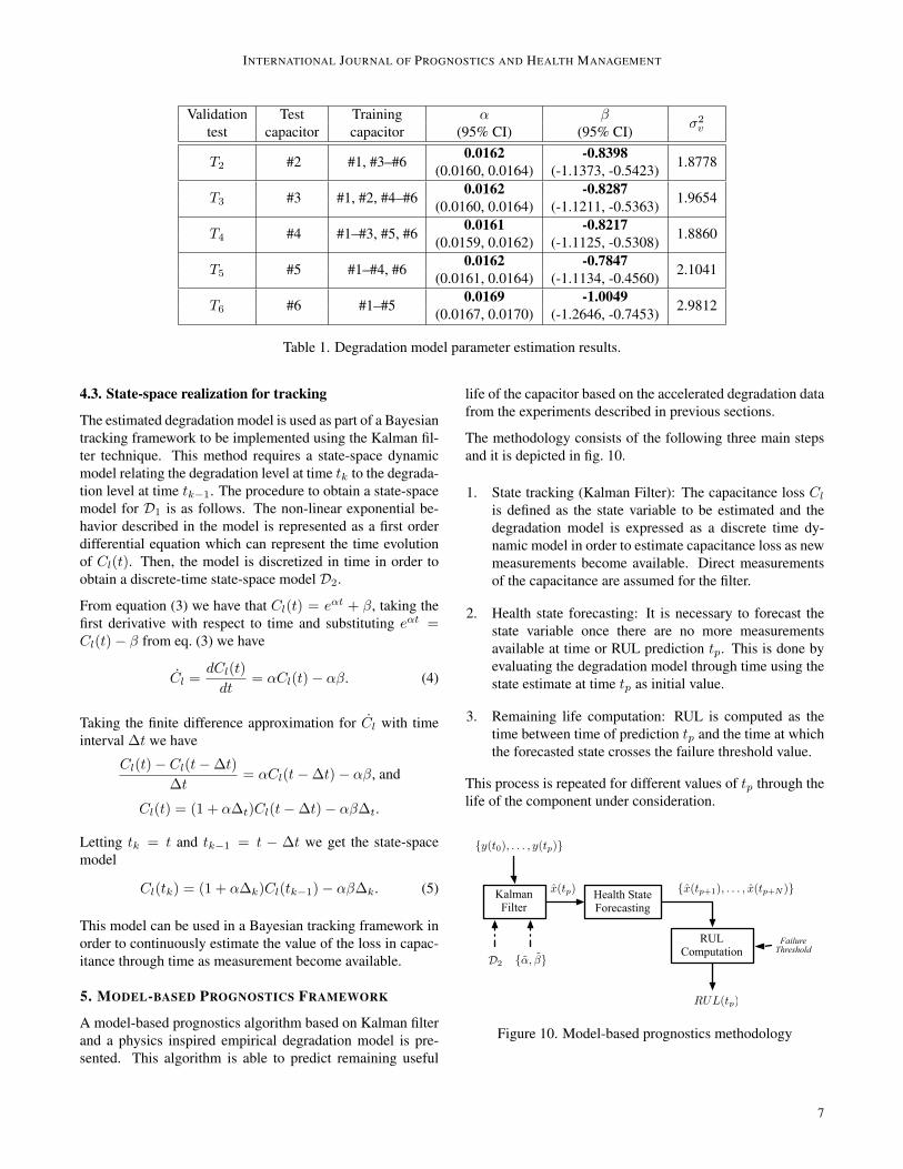
In order to estimate the model parameters, five capacitors areused for estimation, and the remaining capacitor is used totest the prognostics algorithm. This results in six leave-one-out test cases for validation of the prognostics algorithm re-sults. A nonlinear least-squares regression algorithm is usedto estimate the model parameters. Table 1 presents definitionof the test cases and the parameter estimation results. Theestimate and 95% confidence interval is presented for param-eters α and β. In addition, the error variance is included as away to assess the quality of the fit.

Figure 9 shows the estimation results for test case T6. The ex-perimental data are presented together with results from theexponential fit function. It can be observed from the residualsthat the estimation error increases with time. This is to be ex-pected since the last data point measured for all the capacitorsfall slightly off the concave exponential model.

0 50 100 150 200−50

0

50

Cap. lo

ss (

%)

Aging time (hr)

Data

Fit

0 50 100 150 200−10

0

10

Resi

duals

(%

)

Aging time (hr)

Residuals

Figure 9. Estimation results for the empirical degradationmodel.

It should be noted that this degradation model with static pa-rameters will be used in a Bayesian tracking framework. Thiswill help to overcome the degradation model limitation to rep-resent the behavior close to the failure threshold given thetracking framework ability to compensate the estimation asmeasurements become available.

6


Validation Test Training α βσ2vtest capacitor capacitor (95% CI) (95% CI)

T2 #2 #1, #3–#6 0.0162 -0.8398 1.8778(0.0160, 0.0164) (-1.1373, -0.5423)

T3 #3 #1, #2, #4–#6 0.0162 -0.8287 1.9654(0.0160, 0.0164) (-1.1211, -0.5363)

T4 #4 #1–#3, #5, #6 0.0161 -0.8217 1.8860(0.0159, 0.0162) (-1.1125, -0.5308)

T5 #5 #1–#4, #6 0.0162 -0.7847 2.1041(0.0161, 0.0164) (-1.1134, -0.4560)

T6 #6 #1–#5 0.0169 -1.0049 2.9812(0.0167, 0.0170) (-1.2646, -0.7453)

Table 1. Degradation model parameter estimation results.

4.3. State-space realization for tracking

The estimated degradation model is used as part of a Bayesiantracking framework to be implemented using the Kalman fil-ter technique. This method requires a state-space dynamicmodel relating the degradation level at time tk to the degrada-tion level at time tk−1. The procedure to obtain a state-spacemodel for D1 is as follows. The non-linear exponential be-havior described in the model is represented as a first orderdifferential equation which can represent the time evolutionof Cl(t). Then, the model is discretized in time in order toobtain a discrete-time state-space model D2.

From equation (3) we have that Cl(t) = eαt + β, taking thefirst derivative with respect to time and substituting eαt =Cl(t)− β from eq. (3) we have

Cl =dCl(t)

dt= αCl(t)− αβ. (4)

Taking the finite difference approximation for Cl with timeinterval ∆t we have

Cl(t)− Cl(t−∆t)

∆t= αCl(t−∆t)− αβ, and

Cl(t) = (1 + α∆t)Cl(t−∆t)− αβ∆t.

Letting tk = t and tk−1 = t − ∆t we get the state-spacemodel

Cl(tk) = (1 + α∆k)Cl(tk−1)− αβ∆k. (5)

This model can be used in a Bayesian tracking framework inorder to continuously estimate the value of the loss in capac-itance through time as measurement become available.

5. MODEL-BASED PROGNOSTICS FRAMEWORK

A model-based prognostics algorithm based on Kalman filterand a physics inspired empirical degradation model is pre-sented. This algorithm is able to predict remaining useful

life of the capacitor based on the accelerated degradation datafrom the experiments described in previous sections.

The methodology consists of the following three main stepsand it is depicted in fig. 10.

1. State tracking (Kalman Filter): The capacitance loss Clis defined as the state variable to be estimated and thedegradation model is expressed as a discrete time dy-namic model in order to estimate capacitance loss as newmeasurements become available. Direct measurementsof the capacitance are assumed for the filter.

2. Health state forecasting: It is necessary to forecast thestate variable once there are no more measurementsavailable at time or RUL prediction tp. This is done byevaluating the degradation model through time using thestate estimate at time tp as initial value.

3. Remaining life computation: RUL is computed as thetime between time of prediction tp and the time at whichthe forecasted state crosses the failure threshold value.

This process is repeated for different values of tp through thelife of the component under consideration.

KalmanFilter

Health State Forecasting

RULComputation

RUL(tp)

α, βD2

x(tp)

y(t0), . . . , y(tp)

x(tp+1), . . . , x(tp+N )

FailureThreshold

Figure 10. Model-based prognostics methodology

7


5.1. Kalman filter for state estimation

A state-space dynamic model is needed for the filtering. Thestate variable xk at time tk is defined as the percentage ca-pacitance loss Cl(k). Since the system measurements arepercentage loss in capacitance as well, the output equationis given by yk = hxk, where the value of h is equal to one.The following system structure is used in the implementationof the filtering and the prediction using the Kalman filter.

xk = Akxk−1 +Bku+ v,yk = hxk + w,

(6)

where,

Ak = (1 + ∆k),Bk = −αβ∆k,h = 1,u = 1.

(7)

The time increment between measurements ∆k is not con-stant since measurements were taken at non-uniform sam-pling rate. This implies that some of the parameters of themodel in equation (6) will change through time. Furthermore,v and w are normal random variables with zero mean and Qand R variance respectively. The description of the Kalmanfiltering algorithm is omitted from this article. A thoroughdescription of the algorithm can be found in Stengel (1994),a description of how the algorithm is used for forecasting canbe found in Chatfield (2003) and an example of its usage forprognostics can be found in (Saha et al., 2009).

5.2. Future state forecasting

The use of the Kalman filter as a RUL forecasting algorithmrequires the evolution of the state without updating the errorcovariance matrix and the posterior of the state vector. The nstep ahead forecasting equation for the Kalman filter is givenbelow. The last update is done at the time of the last measure-ment tl.

xl+n = Anxl +

n−1∑i=0

AiB (8)

The subscripts from parameters A and B are omitted since aconstant ∆t is used in the forecasting mode (one predictionevery hour).

5.3. Noise models

The model noise variance Q was estimated from the modelregression residuals for each test case as presented in table 1.This variance was used for the model noise in the Kalmanfilter implementation. The measurement noise variance R isalso required in the filter implementation. This variance wascomputed from the direct measurements of the capacitancewith the EIS equipment, the observed variance is 4.99×10−7.

6. PREDICTION OF REMAINING USEFUL LIFE RESULTS

Estate estimation and RUL prediction results are discussedfor test case T6. Figure 11 shows the result of the filter track-ing the complete degradation signal. The residuals show anincreased error with aging time. This is to be expected giventhe results observed from the model estimation process.

0 50 100 150 2000

20

40

Aging time (hr)

Capacit

ance l

oss

(%

)

Observed

Filtered

0 50 100 150 200−5

0

5

Resi

duals

(%

)Aging time (hr)

Figure 11. Tracking results for the Kalman filter implemen-tation applied to test capacitor (capacitor #6).

Figure 12 presents results from the remaining useful life pre-diction algorithm at time tp = 161 (hr), which is the timeat which ESR and C measurements are taken. The failurethreshold is considered to be a crisp value of 20% decrease incapacitance. End of life (EOL) is defined as the time at whichthe forecasted percentage capacity loss trajectory crosses theEOL threshold. Therefore, RUL is EOL minus 161 hours.

0 50 100 150 2000

5

10

15

20

25

Aging time (hr)

Cap

acit

ance

loss

(%

)

Measured

Filtered

Predicted

Failure Threshold

Figure 12. Remaining useful life prediction at time 149 (hr).

Figure 13 presents the capacitance loss estimation and EOLprediction at different points during the aging time. Predic-

8


tions are made after each point in which measurements areavailable. It can be observed that the predictions become bet-ter as the prediction is made closer to the actual EOL. This ispossible because the estimation process has more informationto update the estimates as it nears EOL. Figure 14 presents azoomed-in version of figure 13 focusing in the area close tothe failure threshold.

0 50 100 150 2000

10

20

Measured Filtered Predicted

0 50 100 150 2000

10

20

0 50 100 150 2000

10

20

0 50 100 150 2000

10

20

0 50 100 150 2000

10

20

0 50 100 150 2000

10

20

0 50 100 150 2000

10

20

0 50 100 150 2000

10

20

0 50 100 150 2000

10

20

0 50 100 150 2000

10

20

Aging time (hr)

tp = 0

tp = 24

tp = 47

tp = 71

tp = 94

tp = 116

tp = 139

tp = 149

tp = 161

tp = 171

Figure 13. T6: Health state estimation and forecasting of ca-pacitance loss (%) at different times tp during the aging time;tp = [0, 24, 47, 71, 94, 116, 139, 149, 161, 171].

9


140 150 160 170 180 190

10

20


140 150 160 170 180 190

10

20

140 150 160 170 180 190

10

20

140 150 160 170 180 190

10

20

140 150 160 170 180 190

10

20

140 150 160 170 180 190

10

20

140 150 160 170 180 190

10

20

140 150 160 170 180 190

10

20

140 150 160 170 180 190

10

20

140 150 160 170 180 190

10

20

Aging time (hr)

tp = 0

tp = 24

tp = 47

tp = 71

tp = 94

tp = 116

tp = 139

tp = 149

tp = 161

tp = 171

Figure 14. T6: Detail of the health state estimation and fore-casting of capacitance loss (%) at different times tp during theaging time; tp = [0, 24, 47, 71, 94, 116, 139, 149, 161, 171].

An α-λ prognostics performance metric is presented in Fig-ure 15 for validation test T6. The blue line represents groundtruth and the shaded region is corresponding to a 30% (α =0.3) error bound in the RUL prediction. This metric specifiesthat the prediction is within the error bound halfway betweenfirst prediction and EOL (λ = 0.5). In addition, this metricallows us to visualize how the RUL prediction performancechanges as data closer to EOL becomes available. AppendixB presents the α-λ metric plots for the remaining validationcases.

0 50 100 150 2000

50

100

150

200

250

Time

RU

L

RU L∗(1 ± α)RU L∗T6

Figure 15. Performance based on α-λ performance metric.

6.1. Validation tests

Table 2 summarizes results for the remaining life predictionat all points in time where measurements are available. Thelast column indicates the RUL prediction error. The magni-tude of the error decreases as the prediction time gets closerto EOL. The decrease is not monotonic which is to be ex-pected when using a tracking framework to estimate healthstate because the last point of estimation is used to start theforecasting process.

Table 3 shows performance based on the relative accuracy(RA) metric in equation (9). These metrics allows for an as-sessment of the percentage accuracy relative to the ground-truth value. RA values of 100 represent perfect accuracy. TheRA is presented for all the test cases for different predictiontimes. The last column of the Table 3 represents the me-dian RA of all the test cases for a particular prediction time.It is observed that the RA values decrease considerably fortp = 171. This is consistent with previous observations indi-cating that the algorithm with a fixed-parameter model is notable to cope with the sudden jump in exponential behaviorpresent around the 171 hour. This is a limitation that couldbe overcome by either an enhanced degradation model or aan online estimation of degradation model parameters usinga more sophisticated Bayesian tracking method like extended

10


tp RUL∗ RUL′

T2 RUL′

T3 RUL′

T4 RUL′

T5 RUL′

T6

24 151.04 158.84 164.88 158.76 167.76 159.8947 128.04 131.32 134.08 128.35 135.32 125.9171 104.04 117.01 119.88 115.37 122.63 116.4194 81.04 92.69 96.64 93.09 97.6 95.42

116 59.04 67.28 65.39 67.77 69.5 65.71139 36.04 44.01 44.72 46.88 49.4 53.75149 26.04 30.67 32.41 33.55 35.92 39.95161 14.04 17.23 18.28 18.2 22.64 25.6171 4.04 1.07 2.89 N/A 5.52 8.45

Table 2. Summary of RUL forecasting results.

Kalman filter or particle filter.

RA = 100

(1− RUL∗ −RUL′

RUL∗

)(9)

tp RAT2 RAT3 RAT4 RAT5 RAT6 RA

24 94.8 95.5 91.9 96.9 99.7 95.547 97.4 99.3 96.4 96.7 91.7 96.771 87.5 91.9 84.5 94.1 97.1 91.994 85.6 90 78.9 94.8 94.2 90

116 86 99.1 76.5 98 96.2 96.2139 77.8 95.8 53.1 96.7 81.1 81.1149 82.1 98.4 46.9 94.8 86.6 86.6161 77.2 87.3 16.6 87.5 89.8 87.3171 26.6 26.4 N/A 34.8 63.7 30.7

Table 3. Validation based on relative accuracy metric.

7. CONCLUSION

This paper presents a RUL prediction algorithm based on ac-celerated life test data and an empirical degradation model.The main contributions of this work are: a) the identificationof the lumped-parameter model (Figure 4) for a real capaci-tor as a viable reduced-order model for prognostics-algorithmdevelopment; b) the identification of the ESR and C modelparameters as precursor of failure features; c) the develop-ment of an empirical degradation model based on acceleratedlife test data which accounts for shifts in capacitance as afunction of time; d) the implementation of a Bayesian basedhealth state tracking and remaining useful life prediction al-gorithm based on the Kalman filtering framework. One majorcontribution of this work is the prediction of remaining usefullife for capacitors as new measurements become available.

This capability increases the technology readiness level ofprognostics applied to electrolytic capacitors. The results pre-sented here are based on accelerated life test data and on theaccelerated life timescale. Further research will focus on de-

velopment of functional mappings that will translate the ac-celerated life timescale into real usage conditions time-scale,where the degradation process dynamics will be slower, andsubject to several types of stresses. The performance of theproposed exponential-based degradation model is satisfactoryfor this study based on the quality of the model fit to the ex-perimental data and the RUL prediction performance as com-pared to ground truth. As part of future work we will alsofocus on the exploration of additional models based on thephysics of the degradation process and larger sample size foraged devices. Additional experiments are currently underwayto increase the number of test samples. This will greatly en-hance the quality of the model, and guide the exploration ofadditional degradation-models, where the loading conditionsand the environmental conditions are also accounted for to-wards degradation dynamics.

ACKNOWLEDGMENT

This work was funded by the NASA Aviation Safety Pro-gram, SSAT project.

NOMENCLATURE

CI Ideal capacitance value for an ideal capacitorCR Real capacitor value for a non-ideal capacitor

modelRE Equivalent series resistance of the capacitorCl(k) Capacitance percentage loss at time tkTi Validation test on capacitor iMi Nominal model for a component or systemDi Degradation model for a capacitorRL Load resistance on electrical overstress systemVL Load voltage on electrical overstress systemVo Electrical overstress voltage in aging systemZI Ideal capacitor impedanceZ Capacitor impedance for non-ideal capacitor

modelM1

11


REFERENCES

Bhatti, U., & Ochieng, W. (2007). Failure modes and modelsfor integrated gps/ins systems. The Journal of Naviga-tion, 60, 327.

Celaya, J., Kulkarni, C., Biswas, G., & Goebel, K. (2011a). Amodel-based prognostics methodology for electrolyticcapacitors based on electrical overstress accelerated ag-ing. Proceedings of Annual Conference of the PHMSociety, September 25-29, Montreal, Canada.

Celaya, J., Kulkarni, C., Biswas, G., & Goebel, K. (2011b,March). Towards prognostics of electrolytic capaci-tors. In AIAA 2011 Infotech@Aerospace Conference.St. Louis, MO.

Celaya, J., Kulkarni, C., Biswas, G., & Goebel, K. (2012).Prognostic and experimental techniques for electrolyticcapacitor health monitoring. The Annual Reliabilityand Maintainability Symposium (RAMS), January 23-36, Reno, Nevada..

Chatfield, C. (2003). The analysis of time series: An intro-duction (6th ed.). Chapman and Hall/CRC.

Goodman, D., Hofmeister, J., & Judkins, J. (2007). Elec-tronic prognostics for switched mode power supplies.Microelectronics Reliability, 47(12), 1902-1906. (doi:DOI: 10.1016/j.microrel.2007.02.021)

Gu, J., Azarian, M. H., & Pecht, M. G. (2008). Fail-ure prognostics of multilayer ceramic capacitors intemperature-humidity-bias conditions. In Prognosticsand health management, 2008. phm 2008. interna-tional conference on (p. 1-7).

IEC. (2007-03). 60384-4-1 fixed capacitors for use in elec-tronic equipment (Tech. Rep.).

Judkins, J. B., Hofmeister, J., & Vohnout, S. (2007). A prog-nostic sensor for voltage regulated switch-mode powersupplies. In Aerospace conference, 2007 ieee (p. 1-8).

Kulkarni, C., Biswas, G., Bharadwaj, R., & Kim, K. (2010).Effects of degradation in dc-dc converters on avionicssystems: A model based approach. Machinery FailurePrevention Technology Conference, MFPT 2010.

Kulkarni, C., Biswas, G., & Koutsoukos, X. (2009). A prog-nosis case study for electrolytic capacitor degradationin dc-dc converters. Annual Conference of the Prog-nostics and Health Management Soceity, PHM 2009.

Kulkarni, C., Biswas, G., Koutsoukos, X., Celaya, J., &Goebel, K. (2010). Integrated diagnostic/prognosticexperimental setup for capacitor degradation and healthmonitoring. In 2010 IEEE AUTOTESTCON (p. 1-7).

Kulkarni, C., Biswas, G., Koutsoukos, X., Goebel, K., &Celaya, J. (2010a). Experimental studies of ageing inelectrolytic capacitors. Annual Conference of the Prog-nostics and Health Management Soceity.

Kulkarni, C., Biswas, G., Koutsoukos, X., Goebel, K., &Celaya, J. (2010b). Physics of Failure Models for Ca-pacitor Degradation in DC-DC Converters. The Main-

tenance and Reliability Conference, MARCON 2010.MIL-C-62F. (2008). General specification for capacitors,

fixed, electrolytic.Nie, L., Azarian, M. H., Keimasi, M., & Pecht, M.

(2007). Prognostics of ceramic capacitor temperature-humidity-bias reliability using mahalanobis distanceanalysis. Circuit World, 33(3), 21 - 28.

Orsagh, R., Brown, D., Roemer, M., Dabnev, T., & Hess,A. (2005). Prognostic health management for avionicssystem power supplies. In Aerospace conference, 2005ieee (p. 3585-3591).

Saha, B., Goebel, K., & Christophersen, J. (2009). Compar-ison of prognostic algorithms for estimating remaininguseful life of batteries. Transactions of the Institute ofMeasurement and Control, 31(3-4), 293-308.

Stengel, R. F. (1994). Optimal control and estimation. DoverBooks on Advanced Mathematics.

Jose R. Celaya is a research scientist with SGT Inc. atthe Prognostics Center of Excellence, NASA Ames ResearchCenter. He received a Ph.D. degree in Decision Sciences andEngineering Systems in 2008, a M. E. degree in OperationsResearch and Statistics in 2008, a M. S. degree in ElectricalEngineering in 2003, all from Rensselaer Polytechnic Insti-tute, Troy New York; and a B. S. in Cybernetics Engineeringin 2001 from CETYS University, Mexico.

Chetan S. Kulkarni is a Ph.D candidate at ISIS, VanderbiltUniversity. He received the M.S. degree in EECS from Van-derbilt University, Nashville, TN, in 2009 and a B. E. in Elec-tronics and Electrical Engineering in 2002 from the Univer-sity of Pune, India.

Kai Goebel received the degree of Diplom-Ingenieur fromthe Technische Universitt Mnchen, Germany in 1990. He re-ceived the M.S. and Ph.D. from the University of Californiaat Berkeley in 1993 and 1996, respectively. Dr. Goebel isa senior scientist at NASA Ames Research Center where heleads the Diagnostics and Prognostics groups in the Intelli-gent Systems division. In addition, he directs the PrognosticsCenter of Excellence and he is the technical lead for Prog-nostics and Decision Making of NASAs System-wide Safetyand Assurance Technologies Program. He worked at Gen-eral Electrics Corporate Research Center in Niskayuna, NYfrom 1997 to 2006 as a senior research scientist. He has car-ried out applied research in the areas of artificial intelligence,soft computing, and information fusion. His research interestlies in advancing these techniques for real time monitoring,diagnostics, and prognostics. He holds 15 patents and haspublished more than 200 papers in the area of systems healthmanagement.

Gautam Biswas received the Ph.D. degree in computer sci-ence from Michigan State University, East Lansing. He is aProfessor of Computer Science and Computer Engineering inthe Department of Electrical Engineering and Computer Sci-

12


ence, Vanderbilt University, Nashville, TN.

13


A PROGNOSTICS VALIDATION RESULTS

0 50 100 150 2000

10

20


0 50 100 150 2000

10

20

0 50 100 150 2000

10

20

0 50 100 150 2000

10

20

0 50 100 150 2000

10

20

0 50 100 150 2000

10

20

0 50 100 150 2000

10

20

0 50 100 150 2000

10

20

0 50 100 150 2000

10

20

0 50 100 150 2000

10

20

Aging time (hr)

tp = 0

tp = 24

tp = 47

tp = 71

tp = 94

tp = 116

tp = 139

tp = 149

tp = 161

tp = 171


140 150 160 170 180 190 200

10

20


140 150 160 170 180 190 200

10

20

140 150 160 170 180 190 200

10

20

140 150 160 170 180 190 200

10

20

140 150 160 170 180 190 200

10

20

140 150 160 170 180 190 200

10

20

140 150 160 170 180 190 200

10

20

140 150 160 170 180 190 200

10

20

140 150 160 170 180 190 200

10

20

140 150 160 170 180 190 200

10

20

Aging time (hr)

tp = 0

tp = 24

tp = 47

tp = 71

tp = 94

tp = 116

tp = 139

tp = 149

tp = 161

tp = 171


14


0 50 100 150 2000

10

20


0 50 100 150 2000

10

20

0 50 100 150 2000

10

20

0 50 100 150 2000

10

20

0 50 100 150 2000

10

20

0 50 100 150 2000

10

20

0 50 100 150 2000

10

20

0 50 100 150 2000

10

20

0 50 100 150 2000

10

20

0 50 100 150 2000

10

20

Aging time (hr)

tp = 0

tp = 24

tp = 47

tp = 71

tp = 94

tp = 116

tp = 139

tp = 149

tp = 161

tp = 171


140 150 160 170 180 190 200

10

20


140 150 160 170 180 190 200

10

20

140 150 160 170 180 190 200

10

20

140 150 160 170 180 190 200

10

20

140 150 160 170 180 190 200

10

20

140 150 160 170 180 190 200

10

20

140 150 160 170 180 190 200

10

20

140 150 160 170 180 190 200

10

20

140 150 160 170 180 190 200

10

20

140 150 160 170 180 190 200

10

20

Aging time (hr)

tp = 0

tp = 24

tp = 47

tp = 71

tp = 94

tp = 116

tp = 139

tp = 149

tp = 161

tp = 171


15


0 50 100 150 2000

10

20


0 50 100 150 2000

10

20

0 50 100 150 2000

10

20

0 50 100 150 2000

10

20

0 50 100 150 2000

10

20

0 50 100 150 2000

10

20

0 50 100 150 2000

10

20

0 50 100 150 2000

10

20

0 50 100 150 2000

10

20

0 50 100 150 2000

10

20

Aging time (hr)

tp = 0

tp = 24

tp = 47

tp = 71

tp = 94

tp = 116

tp = 139

tp = 149

tp = 161

tp = 171


140 150 160 170 180 190 200

10

20


140 150 160 170 180 190 200

10

20

140 150 160 170 180 190 200

10

20

140 150 160 170 180 190 200

10

20

140 150 160 170 180 190 200

10

20

140 150 160 170 180 190 200

10

20

140 150 160 170 180 190 200

10

20

140 150 160 170 180 190 200

10

20

140 150 160 170 180 190 200

10

20

140 150 160 170 180 190 200

10

20

Aging time (hr)

tp = 0

tp = 24

tp = 47

tp = 71

tp = 94

tp = 116

tp = 139

tp = 149

tp = 161

tp = 171


16


0 50 100 150 2000

10

20


0 50 100 150 2000

10

20

0 50 100 150 2000

10

20

0 50 100 150 2000

10

20

0 50 100 150 2000

10

20

0 50 100 150 2000

10

20

0 50 100 150 2000

10

20

0 50 100 150 2000

10

20

0 50 100 150 2000

10

20

0 50 100 150 2000

10

20

Aging time (hr)

tp = 0

tp = 24

tp = 47

tp = 71

tp = 94

tp = 116

tp = 139

tp = 149

tp = 161

tp = 171


140 150 160 170 180 190 200

10

20


140 150 160 170 180 190 200

10

20

140 150 160 170 180 190 200

10

20

140 150 160 170 180 190 200

10

20

140 150 160 170 180 190 200

10

20

140 150 160 170 180 190 200

10

20

140 150 160 170 180 190 200

10

20

140 150 160 170 180 190 200

10

20

140 150 160 170 180 190 200

10

20

140 150 160 170 180 190 200

10

20

Aging time (hr)

tp = 0

tp = 24

tp = 47

tp = 71

tp = 94

tp = 116

tp = 139

tp = 149

tp = 161

tp = 171


17


A PROGNOSTICS ALPHA-LAMBDA PERFORMANCEMETRIC

0 50 100 150 2000

50

100

150

200

250

Time

RU

L


Figure 24. T2: Alpha-Lambda Prognostics Metric (λ = 0.5and α = 0.3).

0 50 100 150 2000

50

100

150

200

250

Time

RU

L



0 50 100 150 2000

50

100

150

200

250

Time

RU

L



0 50 100 150 2000

50

100

150

200

250

Time

RU

L



18

2012 EPHM

Towards A Model-based Prognostics Methodology for Electrolytic Capacitors: A Case

Study Based on Electrical Overstress Accelerated Aging

José R. Celaya1, Chetan Kulkarni2, Gautam Biswas2 and Kai Goebel3

1SGT Inc., Prognostics Center of Excellence, NASA Ames Research Center

2ISIS, Vanderbilt University 3Prognostics Center of Excellence, NASA Ames Research Center

1

2012 EPHM

•  Motivation and background •  Prognostics approach •  Accelerated aging experiments •  Degradation modeling •  Prognostics method and results •  Discussion

2

Outline

2012 EPHM

•  Electronic components have increasingly critical role in on-board, autonomous functions for –  Vehicle controls, communications, navigation, radar systems

•  Future aircraft systems will rely more on electronic components

•  Assumption of new functionality increases number of electronics faults with perhaps unanticipated fault modes

3

Motivation

Component : Capacitors, MOSFETs

Line Replaceable Unit (LRU) : Power Supply

Images courtesy : Boeing

•  We need understanding of behavior of deteriorated components to develop capability to anticipate failures/predict remaining RUL

2012 EPHM

Prognostics Research Approach for Electronics

4

2012 EPHM

Model-based prognostics (1/3)

KalmanFilter


RULComputation

RUL(tp)

α, βD2

x(tp)

y(t0), . . . , y(tp)

x(tp+1), . . . , x(tp+N )

FailureThreshold

•  State vector includes dynamics of the degradation process

•  It might include nominal operation dynamics

•  EOL defined at time in which performance variable cross failure threshold

•  Failure threshold could be crisp or also a random variable

5

x(t) = f(x(t), u(t)) + w(t)

y(t) = h(x(t)), u(t)) + v(k)

R(tp) = tEOL − tp

2012 EPHM

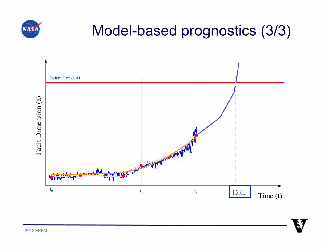
Model-based prognostics (2/3) •  Tracking of health

state based on measurements

•  Forecasting of health state until failure threshold is crossed

•  Compute RUL as function of EOL defined at time failure threshold is crossed

6

110 120 130 140 150 160 170 180 1905

10

15

20

MeasuredFilteredPredicted

110 120 130 140 150 160 170 180 1905

10

15

20

110 120 130 140 150 160 170 180 1905

10

15

20

110 120 130 140 150 160 170 180 1905

10

15

20

Aging time (hr)

tp=116

tp=139

tp=149

tp=161

2012 EPHM

Model-based prognostics (3/3)

tP tD Time (t)

Faul

t Dim

ensio

n (a

)

t0

Failure Threshold

EoL

2012 EPHM

Accelerated Aging

Degradation Modeling

Training Trajectories

Test Trajectory

Parameter Estimation

State-space Representation

Prognostics

DynamicSystem

Realization

Health State Estimation

RUL Estimation

αi, βi

D

D

8

Methodology

xk = Axk−1 +Buk−1 + wk−1

yk = Hxk + vk

KalmanFilter


RULComputation

RUL(tp)

α, βD2

x(tp)

y(t0), . . . , y(tp)

x(tp+1), . . . , x(tp+N )

FailureThreshold

2012 EPHM

Accelerated Aging Systems for Prognostics

9

2012 EPHM

Electrical Overstress Aging System

10 !

!

2012 EPHM

Real Capacitor

EIS

Reduced order model

Degradation model (time)

Health state

estimation

RUL prediction

11

Methodology

!

!

Ck = e!tk +"

2012 EPHM

Dynamic modeling of the degradation process

12

2012 EPHM

•  Based on observed degradation from capacitance parameter

•  Using training capacitor data to estimate degradation model parameters

•  Assumed exponential model based on capacitance loss

•  Parameter estimation with least-squared regression

13

Empirical degradation model

Ck = e!tk +"

2012 EPHM

Degradation model results

14

•  The optimal parameter presented along the 95% confidence interval. •  The residuals are modeled as a normally distributed random variable with zero

mean and variance


Validation Test Training α βσ2vtest capacitor capacitor (95% CI) (95% CI)

T2 #2 #1, #3–#6 0.0162 -0.8398 1.8778(0.0160, 0.0164) (-1.1373, -0.5423)

T3 #3 #1, #2, #4–#6 0.0162 -0.8287 1.9654(0.0160, 0.0164) (-1.1211, -0.5363)

T4 #4 #1–#3, #5, #6 0.0161 -0.8217 1.8860(0.0159, 0.0162) (-1.1125, -0.5308)

T5 #5 #1–#4, #6 0.0162 -0.7847 2.1041(0.0161, 0.0164) (-1.1134, -0.4560)

T6 #6 #1–#5 0.0169 -1.0049 2.9812(0.0167, 0.0170) (-1.2646, -0.7453)

Table 1. Degradation model parameter estimation results.

Figure 9 shows the estimation results for test case T6. The ex-perimental data are presented together with results from theexponential fit function. It can be observed from the residualsthat the estimation error increases with time. This is to be ex-pected since the last data point measured for all the capacitorsfall slightly off the concave exponential model.

0 50 100 150 200!50

0

50

Cap

. lo

ss (

%)

Aging time (hr)

Data

Fit

0 50 100 150 200!10

0

10

Res

idu

als

(%)

Aging time (hr)

Residuals

Figure 9. Estimation results for the empirical degradationmodel.

It should be noted that this degradation model with static pa-rameters will be used in a Bayesian tracking framework. Thiswill help to overcome the degradation model limitation to rep-resent the behavior close to the failure threshold given thetracking framework ability to compensate the estimation asmeasurements become available.

4.3. State-space realization for tracking

The estimated degradation model is used as part of a Bayesiantracking framework to be implemented using the Kalman fil-ter technique. This method requires a state-space dynamicmodel relating the degradation level at time tk to the degrada-

tion level at time tk−1. The procedure to obtain a state-spacemodel for D1 is as follows. The non-linear exponential be-havior described in the model is represented as a first orderdifferential equation which can represent the time evolutionof Cl(t). Then, the model is discretized in time in order toobtain a discrete-time state-space model D2.

From equation (3) we have that Cl(t) = eαt + β, taking thefirst derivative with respect to time and substituting eαt =Cl(t)− β from eq. (3) we have

Cl =dCl(t)

dt= αCl(t)− αβ. (4)

Taking the finite difference approximation for Cl with timeinterval ∆t we have

Cl(t)− Cl(t−∆t)

∆t= αCl(t−∆t)− αβ, and

Cl(t) = (1 + α∆t)Cl(t−∆t)− αβ∆t.

Letting tk = t and tk−1 = t − ∆t we get the state-spacemodel

Cl(tk) = (1 + α∆k)Cl(tk−1)− αβ∆k. (5)

This model can be used in a Bayesian tracking framework inorder to continuously estimate the value of the loss in capac-itance through time as measurement become available.

5. MODEL-BASED PROGNOSTICS FRAMEWORK

A model-based prognostics algorithm based on Kalman filterand a physics inspired empirical degradation model is pre-sented. The methodology consists of the following three mainsteps and it is depicted in fig. 10.

1. State tracking (Kalman Filter): The capacitance loss Cl

is defined as the state variable to be estimated and thedegradation model is expressed as a discrete time dy-namic model in order to estimate capacitance loss as newmeasurements become available. Direct measurementsof the capacitance are assumed for the filter.

7

2012 EPHM

Prognostics method and results

15

2012 EPHM

•  Implementation of prognostics algorithm with Kalman filter

•  Capacitance loss considered as state variable •  EIS measurements and lumped parameter

model used to obtained measured capacitance loss values

•  Empirical degradation model used to generate the state transition equation

•  Use one Capacitor for testing and the rest for model parameter estimation (leave on out test)

•  Failure threshold of 20% drop on capacitance based on MIL-C-62F

16

Prognostics algorithm

2012 EPHM

Kalman filter implementation •  State transition

equation derived from degradation model

•  State-space model for filter implementation

17

!C!t

=!C "!"

Ct "Ct " #t

#t=!Ct " #t "!"

Ct = (1+!#t)Ct " #t "!"#t

Ck = (1+!#k)Ck " 1"!"#k

Ck = AkCk ! 1+Bku+ v!yk = hCk +w,where

Ak = (1+"t),Bk = !!""k,h =1,!u =1.

Ck = e!tk +"

2012 EPHM

•  Assumed measurements are not available at some point in time

•  Filter used in forecasting mode to predict future states

•  Predictions done at 1 hr. intervals •  State transition equation used to propagate

state (n: number of prediction steps, l: last measurement at tl)

18

Prediction mode

Cl+n = AnCl + AiB

i=0

n!1

"

2012 EPHM

Tracking and forecasting (Cap. #6)

19

110 120 130 140 150 160 170 180 1905

10

15

20

MeasuredFilteredPredicted

110 120 130 140 150 160 170 180 1905

10

15

20

110 120 130 140 150 160 170 180 1905

10

15

20

110 120 130 140 150 160 170 180 1905

10

15

20

Aging time (hr)

tp=116

tp=139

tp=149

tp=161

2012 EPHM

Relative Accuracy

20


tp RUL∗ RUL

T2 RUL

T3 RUL

T4 RUL

T5 RUL

T6

24 151.04 158.84 164.88 158.76 167.76 159.8947 128.04 131.32 134.08 128.35 135.32 125.9171 104.04 117.01 119.88 115.37 122.63 116.4194 81.04 92.69 96.64 93.09 97.6 95.42

116 59.04 67.28 65.39 67.77 69.5 65.71139 36.04 44.01 44.72 46.88 49.4 53.75149 26.04 30.67 32.41 33.55 35.92 39.95161 14.04 17.23 18.28 18.2 22.64 25.6171 4.04 1.07 2.89 N/A 5.52 8.45



RA = 100

1− RUL∗ −RUL

RUL∗

(9)

tp RAT2 RAT3 RAT4 RAT5 RAT6RA

24 94.8 95.5 91.9 96.9 99.7 95.5

47 97.4 99.3 96.4 96.7 91.7 96.7

71 87.5 91.9 84.5 94.1 97.1 91.9

94 85.6 90 78.9 94.8 94.2 90

116 86 99.1 76.5 98 96.2 96.2

139 77.8 95.8 53.1 96.7 81.1 81.1

149 82.1 98.4 46.9 94.8 86.6 86.6

161 77.2 87.3 16.6 87.5 89.8 87.3

171 26.6 26.4 N/A 34.8 63.7 30.7


7. CONCLUSION




ACKNOWLEDGMENT


NOMENCLATURE



model M1

11


tp RUL∗ RUL

T2 RUL

T3 RUL

T4 RUL

T5 RUL

T6

24 151.04 158.84 164.88 158.76 167.76 159.8947 128.04 131.32 134.08 128.35 135.32 125.9171 104.04 117.01 119.88 115.37 122.63 116.4194 81.04 92.69 96.64 93.09 97.6 95.42

116 59.04 67.28 65.39 67.77 69.5 65.71139 36.04 44.01 44.72 46.88 49.4 53.75149 26.04 30.67 32.41 33.55 35.92 39.95161 14.04 17.23 18.28 18.2 22.64 25.6171 4.04 1.07 2.89 N/A 5.52 8.45



RA = 100

1− RUL∗ −RUL

RUL∗

(9)


24 94.8 95.5 91.9 96.9 99.7 95.5

47 97.4 99.3 96.4 96.7 91.7 96.7

71 87.5 91.9 84.5 94.1 97.1 91.9

94 85.6 90 78.9 94.8 94.2 90

116 86 99.1 76.5 98 96.2 96.2

139 77.8 95.8 53.1 96.7 81.1 81.1

149 82.1 98.4 46.9 94.8 86.6 86.6

161 77.2 87.3 16.6 87.5 89.8 87.3

171 26.6 26.4 N/A 34.8 63.7 30.7


7. CONCLUSION




ACKNOWLEDGMENT


NOMENCLATURE



model M1

11

2012 EPHM

Discussion

21

2012 EPHM

•  RUL prediction algorithm based on accelerated life test data and an empirical degradation model –  Identification of the lumped-parameter model for a

real capacitor as a viable reduced-order model for prognostics-algorithm development

–  Identification of ESR and C as precursor of failure feature parameters

– Development of an empirical degradation model based on accelerated life test data which accounts for shifts in capacitance as a function of time

–  Implementation of a Bayesian based health state tracking and RUL prediction algorithm based on the Kalman filtering framework

22

Contribution

2012 EPHM

•  Proposed approach requires further development – Results presented over accelerated aging test time

scale – The empirical degradation model can be improved. – Degradation model and prediction algorithm assume

constant loading and environmental conditions – Explore more sophisticated Bayesian tracking

algorithms if required to handle variable loading and operational conditions as well as degradation models with time varying parameters

– Uncertainty representation in the forecasting section and model uncertainty assessment under the Bayesian tracking framework

23

Comments

2012 EPHM

Thank You

This work was funded by NASA, Aviation Safety Program, IVHM and SSAT Projects

24

2012 EPHM

Backup slides

25

2012 EPHM

Results (all)

26

2012 EPHM

RUL Results for all test cases

27


tp RUL∗ RUL

T2 RUL

T3 RUL

T4 RUL

T5 RUL

T6

24 151.04 158.84 164.88 158.76 167.76 159.8947 128.04 131.32 134.08 128.35 135.32 125.9171 104.04 117.01 119.88 115.37 122.63 116.4194 81.04 92.69 96.64 93.09 97.6 95.42

116 59.04 67.28 65.39 67.77 69.5 65.71139 36.04 44.01 44.72 46.88 49.4 53.75149 26.04 30.67 32.41 33.55 35.92 39.95161 14.04 17.23 18.28 18.2 22.64 25.6171 4.04 1.07 2.89 N/A 5.52 8.45



RA = 100

1− RUL∗ −RUL

RUL∗

(9)


24 94.8 95.5 91.9 96.9 99.7 95.5

47 97.4 99.3 96.4 96.7 91.7 96.7

71 87.5 91.9 84.5 94.1 97.1 91.9

94 85.6 90 78.9 94.8 94.2 90

116 86 99.1 76.5 98 96.2 96.2

139 77.8 95.8 53.1 96.7 81.1 81.1

149 82.1 98.4 46.9 94.8 86.6 86.6

161 77.2 87.3 16.6 87.5 89.8 87.3

171 26.6 26.4 N/A 34.8 63.7 30.7


7. CONCLUSION




ACKNOWLEDGMENT


NOMENCLATURE



model M1

11

2012 EPHM

Degradation on lumped parameter model

28

!C and ESR are estimated from EIS measurements

0 20 40 60 80 100 120 140 160 180 2000

10

20

Aging Time (hr)

Cap

acita

nce

(loss

%)

0

20

40

60

ESR

(inc

reas

e %

)

C

ESR

towards a model-based prognostics methodology for ... a model-based prognostics methodology for...

Documents