toward an integrative software infrastructure for - my water quality
TRANSCRIPT
11/23/2011 10:55 AM 1
Toward an integrative software infrastructure for water management in
the Smarter Planet
Barbara Eckman1, Mark Feblowitz
2, Alex Mayer
3, Anton Riabov
4
Abstract
Building the Smarter Planet requires creating an Intelligent Infrastructure that integrates technology
with business, government, and the everyday life of the citizens of earth, to maximize the use of scarce
resources, balance human use and ecosystem preservation, reduce costs, and improve quality of life.
One of the keystones of this Intelligent Infrastructure is an Integrative Modeling Framework (IMF), a
platform to enable the integration by non-expert users of diverse, sensor-based data, related business
data, and complex, cross-disciplinary mathematical modeling, in support of planning, monitoring,
management, reporting, and decision support applications. We describe a research prototype that
applies the Mashup Automation with Runtime Invocation & Orchestration (MARIO) technology from
IBM Research to this problem in a specific application area in water management: simulating stream
discharges using compositions of hydrologic process submodels derived from monolithic stream
discharge simulators. We show how MARIO’s semantic tagging and model composition engine enable
us to meet three critical challenges of an IMF: 1) generating valid chain(s) or compositions of model
components, given a definition of starting and ending states ; 2) allowing all scientifically valid
compositions of components; and 3) disallowing compositions that are scientifically invalid, i.e., that
combine model components whose basic assumptions about quantities like soil architectures or
evaporation schemes conflict. While we focus here on water management , the technology that we
describe is readily generalizable to other Intelligent Infrastructure applications, e.g., cities,
transportation, and utilities.
Introduction
Building the Smarter Planet requires creating an Intelligent Infrastructure that integrates technology
with business, government, and the everyday life of the citizens of earth, to maximize the use of scarce
resources, balance human use and ecosystem preservation, reduce costs, and improve quality of life.
Bringing intelligence to these interactions requires an unprecedented degree of integration of
heterogeneous data, analytics and simulations. One of the keystones of this Intelligent Infrastructure is
therefore an Integrative Modeling Framework (IMF), an infrastructure platform to enable the
integration by non-expert users of diverse, sensor-based data, related business data, and complex,
cross-disciplinary mathematical modeling, in support of planning, monitoring, management, reporting,
1 PO Box X, Wayne, PA 19087; [email protected]
2 IBM T.J. Watson Research Center, Cambridge, MA 02142; [email protected]
3 Michigan Technological University, Houghton, MI 49931; [email protected]
4 IBM T.J. Watson Research Center, Hawthorne, NY 10532; [email protected]

11/23/2011 10:55 AM 2
and decision support applications. For example, critical to the technology foundation for the
development and operation of Smart Cities is the integration of a wide variety and volume of data and
the application of a correspondingly wide variety of analytics and simulations to interpret this data,
make predictions based on it, and optimize business processes that act on it.[1] In the domain of water
management, policy makers and other stakeholders need to assess, come to consensus, and act on land-
use decisions that balance human use and ecosystem preservation/restoration. These decisions require
input from models from a wide variety of environmental sectors, including water balance, water quality,
carbon balance, crop production, and proxies for biodiversity.[2] But model codes are typically written
in a monolithic fashion which does not support building large integrated models out of a set of model
components. Furthermore, in the relatively rare case where codes are modularized, a common
framework is lacking which can provide a consistent interface for passing data, as well as a language in
which to express rules about which components may validly be integrated.
A number of approaches have been developed for integration of data sources and/or services, such as
Service-Oriented Architecture (SOA), Enterprise Service Bus (ESB), Service Component Architecture
(SCA) and Extract, Transform, Load (ETL). All of these technologies are relevant to an integrative
modeling framework and address important needs, providing execution environments, connectivity,
service catalogs, interface contracts, and data transformation. In this paper we present a new approach
to describing components that makes it possible to exclude invalid compositions of model components
based not just on interface contracts but also on semantic constraints. As illustrated in Figure 1, our
approach complements these technologies and can be best applied in combination with all or some of
them.
In this work, we describe a research prototype that applies IBM research technology to the problem of
model integration in a specific application area: simulating stream discharges. We choose this
application area because we have a deep understanding of the needs and issues involved in stream
discharge simulation, and therefore the research technology applied to it will be challenged and
stretched by its requirements. Nevertheless , the technology that we describe is readily generalizable to
other Intelligent Infrastructure applications, e.g., cities, transportation, and utilities.
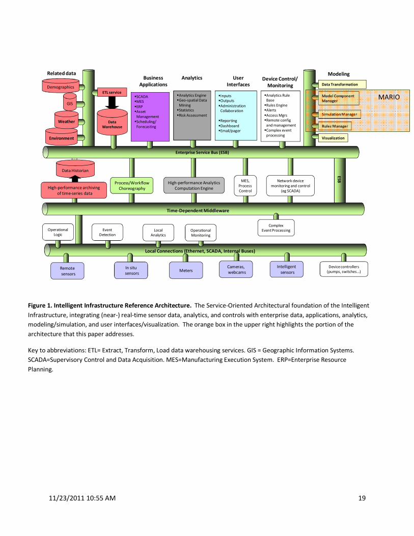
The reference software architecture we propose for an Intelligent Infrastructure is shown in Figure 1, a
variation on that of [3]. A Service-Oriented Architecture, it integrates (near-) real-time sensor data,
analytics, and controls with enterprise data, applications, analytics, modeling/simulation, and user
interfaces/visualization. It comprises three Enterprise Service Buses, specialized for (from bottom to
top): 1) Sensor Level: Event/Data Capture, Analytics, Pattern Recognition, Control; 2) Operational Level:
Business Processes, Workflow, Modeling, Contingencies and Analytics; and 3) Enterprise Level:
Visualization, Simulation, Process Optimization, Planning, Deep Insight. An orange box in the upper
right highlights the portion of the architecture on which this paper focuses: managing model
components and the metadata and rules that govern their composition into workflows or chains of
model components that comprise simulations. To our knowledge, this functionality is lacking in existing
modeling frameworks but it is critical for an Intelligent Infrastructure IMF, particularly one whose target
users are not expert modelers.
11/23/2011 10:55 AM 3
In the specific area of estimating streamflow, there are a variety of well-respected models, each with
different assumptions about such concepts as soil architecture and how best to correct for error in
estimating effective precipitation. We are developing a flexible, extensible modeling framework to
enable non-expert modelers to define and run multi-step analytic simulations for river basin
management, based on the Mashup Automation with Runtime Invocation & Orchestration (MARIO)
project from IBM Research. In this framework, we divide monolithic models into atomic components
with clearly defined semantics encoded via rich metadata representation. Once models and their
semantics and composition rules have been registered with the system by their authors or other
experts, non-expert users may construct simulations as workflows of these atomic model components.
A model composition engine enforces rules/constraints for composing model components into
simulations, to avoid the creation of Frankenmodels, models that execute but produce scientifically
invalid results.
This paper is organized as follows. We begin in the Motivation section by describing the basic concepts
of hydrology and motivating the need for an IMF in that field. Next we describe the Framework for
Understanding Structural Errors (FUSE)[4], a system in which four parent stream discharge models have
been componentized, allowing the components to be assembled into new models. We view this work
both as a case study for the need for an IMF in hydrology (Case Study: FUSE section), and as an excellent
source of model components for our work. Next, we summarize the underlying MARIO technology
(MARIO: A New Approach to Model Integration) and describe how we defined MARIO-ready
composable components based on FUSE, taking advantage of MARIO’s metadata capabilities to
represent necessary constraints on compositions of model components (Applying MARIO to FUSE). Next
we describe the results of this application (Results). The Discussion section highlights what we see as the
primary advantages of our approach, and describes our plans for further research. The Conclusion
summarizes the contributions of the paper.
Motivation
In order to motivate the need for an IMF in the hydrology field, we must first introduce some hydrology
basics.
A Hydrology Primer
Hydrology is the science that encompasses the occurrence, distribution, movement and properties of
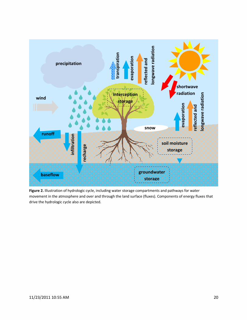
water and the relationship of water with environmental and human systems. The hydrologic cycle is a
continuous process where water is evaporated and transported from the earth's surface to the
atmosphere and back to the land and oceans. Within the hydrologic cycle, water is subjected to physical,
chemical and biological processes as it travels various paths through the atmosphere and the earth's
surface. Figure 2 illustrates some of the processes and storage reservoirs in the hydrologic cycle,
including the principle that energy, via solar radiation, drives the cycling of water between the earth’s
surface and the atmosphere.
Current, critical issues in hydrology include determining how fresh water distribution over and through
and on the land surface may be impacted as a result of climate change and how the cycling of water
11/23/2011 10:55 AM 4
influences patterns of ecosystem carbon and nutrient cycling. Given the intensive nature of human
inter-relationships with the hydrologic cycle, hydrologists and water resources managers are concerned
with adapting water management strategies to variations in the hydrologic cycle, induced by natural or
anthropogenic changes in land cover and climate.
Hydrologic modeling, which encompasses the movement and storage of water through the hydrologic
cycle, can be a powerful tool for exploring issues of interest to hydrologists and water managers. In this
work, we are narrowing the scope to consider models whose primary function is to simulate stream
flows, or discharges, in response to precipitation events (e.g. rain storm or snow melt events), although
we believe our approach to be generally applicable, both to wider hydrologic modeling issues and to
other Intelligent Infrastructure domains. Stream discharge simulations are used to understand and
make predictions concerning water supply availability, including support for water banking and
groundwater recharge, flood events, hydroelectric power generation, and ecosystem interactions, such
as relationships between fish survival and flow magnitude and timing.
Approaches for modeling stream discharge vary widely in terms of how the models conceptually and
mathematically represent the physical processes that govern the distribution and movement of water
over and through the land surface. The models are typically applied over a watershed or basins that can
range in size from a few to millions of square kilometers. Simulations are run over time scales that
range from a matter of minutes to months to years. A typical model development exercise involves
conceptualization of the hydrologic system, definition of the relevant model equations, writing
computer codes, assembly of input information, and calibration of model tuning parameters against
observed discharges. The calibrated models are used to forecast stream discharges under a variety of
climatic or land cover conditions.
The models usually operate by separating precipitation entering the land surface into various fluxes,
such as (1) water that flows on or under the land surface and eventually into a stream channel, (2) water
that evaporates or transpires from the land surface or through vegetation into the atmosphere, and (3)
water that percolates into the underlying groundwater. Model operation also usually involves dividing
the physical system into a number of compartments. Water can be stored within compartments. Water
fluxes describe the movement of water in, out, and between compartments.
Water balance equations are written for each compartment, as in
= −∑ ∑in out
dSq q
dt
where dS dt is the time rate of change of storage, S, of water in a compartment, qin represents the
fluxes of water entering a compartment, and qout represents the fluxes leaving a compartment. The flux
terms typically consist of empirically-derived equations that depend on state variables such as storage
and temperature and empirical parameters. The empirical parameters are usually derived by calibrating
the model against stream discharge observations. Water balance equations typically must be solved
using numerical approximations. A typical model may involve several, coupled water balance equations.
11/23/2011 10:55 AM 5
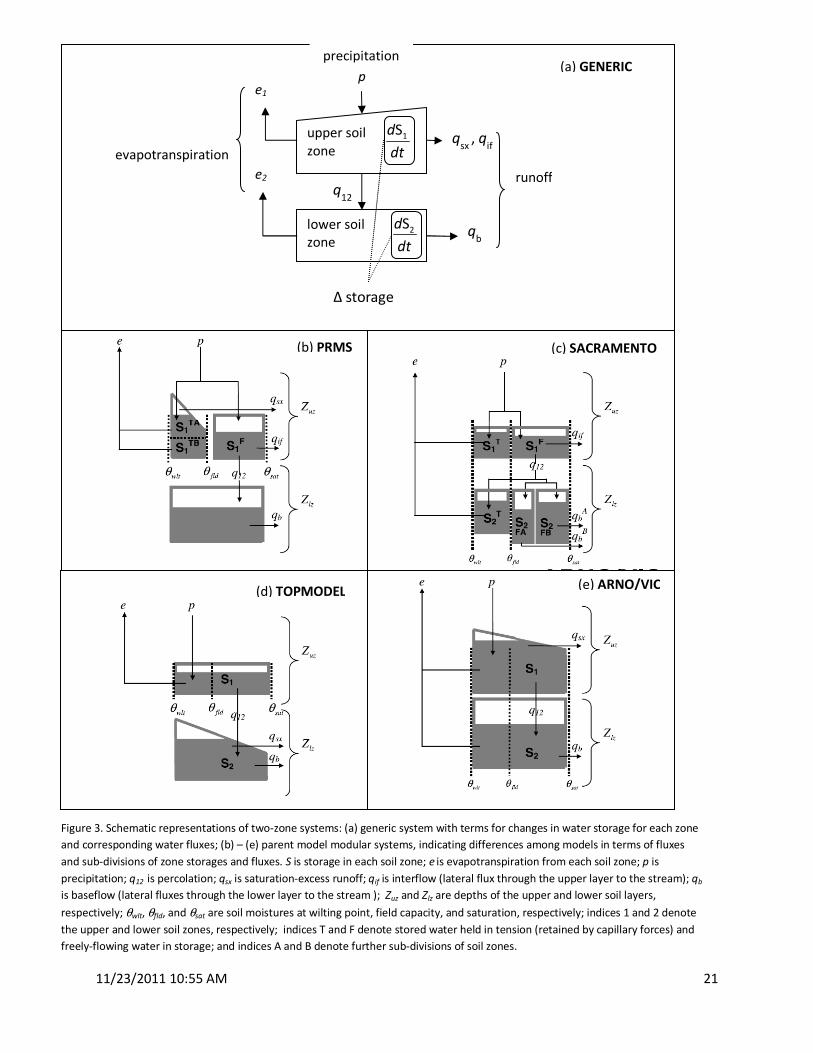
Figure 3 a) shows an example of a model that divides the soil between the land surface and a near-
surface groundwater aquifer into two layers, each with its own water balance equation.
There are many sources of uncertainty involved in the development of stream discharge models,
including errors in the conceptualization of the system. One promising approach to contending with this
uncertainty is to use an ensemble of models to make predictions of streamflows, also known as multi-
modeling. Multi-modeling is attractive in that the ensemble mean of all model outputs combines the
strengths of each model, generating an output that is more robust than a single model,. Combining
model outputs could be as simple as averaging the stream discharges estimated by each model or could
incorporate error estimates obtained during model calibration, as in
=∑ k kF w f
where F is the ensemble mean stream discharge, fk is the result of kth model, and wk is the weight of
the kth model, related to model’s correlation with observations during calibration.
Stream discharge codes, and indeed codes used for other aspects of water management, can be built in
a modular fashion. Code modules can be written for each water balance equation and flux equation,
with the appropriate data being passed between each module. If codes are written in a modular format
and data structures are consistent, modules can be swapped in and out of the models and modules
representing different processes can be added. For example, the system represented in Figure 3 a) does
not include a conceptual representation of canopy interception storage (the part of precipitation that is
captured and held by vegetation). An appropriate canopy interception module would have atmospheric
precipitation as input and would, in principle, output precipitation onto the soil surface and into the
upper soil water balance equation.
Historically, stream discharge model development has occurred through different groups in academic
institutions and government agencies, often with little communication among the groups. As a result,
many models have been developed, each with its strength and weaknesses. In addition, codes have
often been written in a monolithic fashion, and, in the case where codes are modularized, code
structures for passing data are not consistent from model to model. This practice has led to several
inefficiencies, including the need to customize input data to suit each model and to write specialized
code to allow the models or pieces of the models to pass data among each other.
The Need for an Integrative Modeling Framework
To facilitate modeling in the hydrology community and the exchange of modeling ideas and best
practices, it is necessary to provide a flexible, extensible modeling framework infrastructure for defining
and running multi-step analytic simulations, and integrating them with real-time sensor data. This
approach requires the division of extant (typically monolithic) discipline-specific models into atomic
model components. Cross-disciplinary simulations may then be expressed as workflows specified as
chains or compositions of components. Unlike other existing modeling frameworks, our framework is
intended to support non-expert modelers. Since models can be built on different or even conflicting
assumptions and definitions of key terms, not all compositions of components represent scientifically
valid simulations. It is critical not to allow formation of Frankenmodels, compositions of incompatible
11/23/2011 10:55 AM 6
components that produce scientifically invalid simulations. This requires a rich metadata specification
for representing model semantics and expressing rules/constraints for combining model components.
Additional requirements are a software environment for modeling framework development, and an
adapter strategy for non-Java code (e.g., FORTRAN, Python) that still enables efficient simulation runs,
including parallelization of component execution.
An IMF would allow for modules to be written to a published interface and then to be re-assembled to
form completely new models, as long as the structures for passing data in and out of the models were
consistent. Initially this approach would involve extracting component modules from the various parent
stream discharge codes, but we expect that soon model developers will write directly to the interface.
This approach would potentially enhance the robustness of multi-modeling efforts.
Several groups have attempted to develop IMFs for hydrologic modeling. Leavesley et al. [5] developed
the Unix-based Modular Modeling System (MMS) to support development of hydrologic process
algorithms and the integration of user-selected sets of algorithms into operational hydrologic models.
Designed to facilitate integration of existing modelling systems, the OpenMI project focuses on defining
a standardized interface to pass data among models and model components.[6] More recently, the
Consortium of Universities for the Advancement of Hydrologic Science, Inc. (CUAHSI) is launching an
effort towards the development of a Community Hydrologic Modeling Platform (CHyMP). [7] The
general thrust of CHyMP is to promote a community-based effort to develop modular components of
the hydrologic cycle that can be integrated into useful models and modeling and used in advanced
hydrologic research. Clark et al. have developed the Framework for Understanding Structural Errors
(FUSE)[4], which focuses primarily on multi-modeling. In this work, the authors componentized four
parent stream discharge models and manually combined the components into new models. The
following section explains the FUSE methodology.
Case Study: FUSE
In Clark et al.’s FUSE code, individual flux equations are modularized, rather than linking existing sub-
models, as is done in the MMS effort . In FUSE, modeling options are drawn from four parent rainfall-
runoff models (Figure 3 b-e), denoted here as the PRMS, Sacramento, TOPMODEL, and ARNO/VIC
models (see [4] for the full name and citations for each model). The parent models include several
processes that interact with the subsurface, such as vegetation storage, but for simplicity, only fluxes
within the subsurface are considered. In each model, the subsurface is divided into two layers: the
unsaturated layer, or upper soil layer (above the water table), and the saturated layer, or lower soil layer
(below the water table). Each parent model describes the architecture of the upper and lower soil layer
and equations for simulating fluxes: evaporation, surface runoff, percolation of water between soil
layers, interflow, and base flow. The layer architecture refers to the subdivision of the water storage
into from one to three compartments. The equations for simulating fluxes for a given process vary in
terms of the algebraic equations and the parameters and state variables needed to calculate the fluxes.
The parent models are simplified somewhat to allow for as many processes as possible to be
modularized and interchangeable and incorporated into new models that are re-assembled from the
11/23/2011 10:55 AM 7
resulting modules. We used a more recent version of the FUSE code than described in Clark et al., which
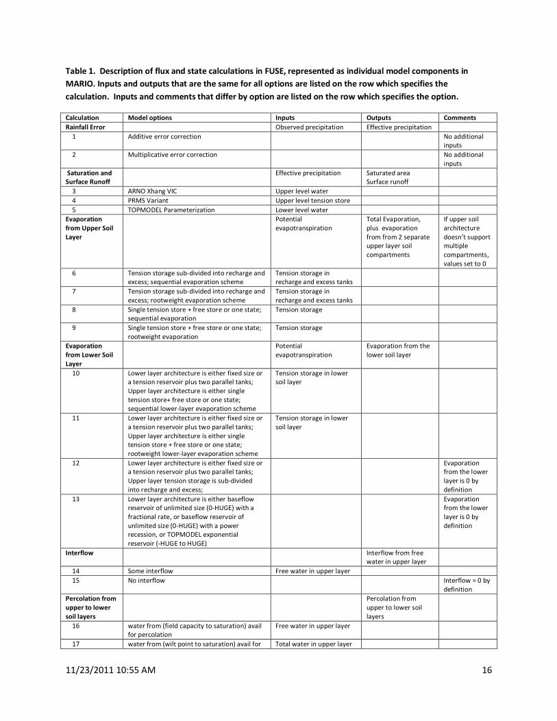
includes several more model building choices. The model building options are given in Table 1. The
number of possible models built by simply choosing one option for each calculation in Table 1 exceeds
250,000. However, the vast majority of model decisions, e.g., selection of flux equations, are tied to
preliminary decisions such as the choice of soil layer architecture. When model compositions are
removed that involve incompatible model components, 316 valid models can be constructed. Note that
in FUSE, scientifically invalid compositions are removed manually using programming constructs such as
loops and CASE statements, while in our IMF these compatibility constraints, once registered, are
automatically enforced by the framework.
The FUSE code is written in FORTRAN. The code is written in a modularized fashion, and data structures
are defined to make the addition of more sub-models relatively straightforward and facilitate
communication between sub-models. User input files determine the model decisions. FORTRAN CASE
statements are used to establish which equations are to be evaluated in the subroutines that calculate
model fluxes and related quantities, given the user’s model building decisions. Since the solution of the
resulting nonlinear ordinary differential equations is not a trivial task, a large portion of the FUSE code is
dedicated to the mathematics required to solve the water balance equations for the state variables. The
FUSE code also is set up to allow either the user to input values of the model parameters or to have the
code estimate the model parameters internally, based on matching simulated and observed stream
discharges.
We build on FUSE in the present paper to show how those components could be assembled into
integrated workflows of components , or model compositions, using a more flexible and powerful
declarative approach that manages both syntactic and semantic heterogeneity. The next section
describes the MARIO project, which forms the basis of our integrated system.
MARIO: A New Approach to Model Integration
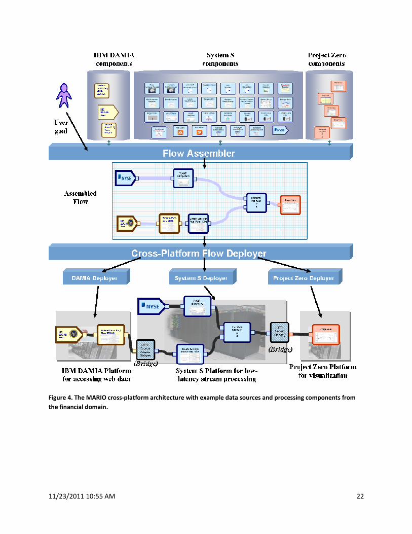
MARIO [8], developed at IBM Research, is an experimental software tool implementing goal-driven,
automated assembly of cross-platform [9], flow-based applications (see Figure 4). A flow-based
application is an assembly of software components – software modules, web services, etc. – that are
interconnected via a dataflow and assembled to perform some information processing task. MARIO’s
ability to interpret component semantic descriptions, and to assemble from them large numbers of
flow-based applications, positions it well as a foundational element of an IMF.
To assemble the individual components into an interconnected application, MARIO requires two things:
1) semantic descriptions of the component’s inputs, outputs, and parameters, and 2) a semantic
description of the goal to be achieved by the application. Component developers provide the
component descriptions, MARIO users (e.g., hydrologists) express their processing goals, and MARIO
assembles the flows based on that information.
11/23/2011 10:55 AM 8
Components in MARIO are described using a light-weight semantic tagging approach formal enough to
support automated assembly yet simple enough to be authored by most developers.5 Component
developers annotate each component’s inputs and outputs with tags, using an XML representation.
Examples (Figure 7) are described in detail in the next section. The tags describe syntax and semantics of
the input or output, including the type of information received or sent, formatting of the data,
measurement units, processing or analysis applied to obtain the data, etc. Input descriptions are used to
specify assembly constraints. In a valid composition, every tag specified in the description of an input
must be present directly or indirectly in the description of the output connected to that input.
MARIO users employ many of the same tags to express processing goals. Using MARIO’s faceted
interface, shown in Figure 6, a hydrologist might browse among various facets of information, in much
the same way he might shop for shoes online, picking the tags that best describe the desired processing
outcome. He could select tags such as ObservedPrecipitation, RoutedRunoff, GraphView; MARIO then
presents a plan for satisfying that goal—a GraphView of a multi-step composition capable of producing
RoutedRunoff, calculated using ObservedPrecipitation as input. The user can examine the composition
and can either deploy it or specify additional constraints by selecting additional tags such as
MultiplicativeRainErrorCalculation until both MARIO’s interpretation of the goal and its selected
composition meet the user’s preferences.
For a given processing goal MARIO identifies combinations of components that satisfy assembly
constraints and jointly produce outputs matching goal tags, doing so by applying a special-purpose,
optimized planning algorithm. If the goal is ambiguous MARIO selects the top-ranked composition, with
ranking based on the total cost and quality of each candidate composition.
Tags in MARIO are typically organized into a “tagsonomy” (Figure 7, top) – a simple taxonomic hierarchy
of tags. In a MARIO tagsonomy, tags are related to other tags using simple “extends” links with a
specific interpretation for component assembly, open to many uses/interpretations by the component
developer.
Composition rules are defined as a combination of match rules and propagation rules. Tags are either
matched directly, as an exact tag name match, or taxonomically, whereby a tag can be matched to any
sub-tag. In a direct match, an input tagged with EffectivePrecipitation could be matched to any output
also tagged with EffectivePrecipitation. For a taxonomic match, an input tagged with
SaturationAndSurfaceRunoff could be matched to an output tagged with any model-specific
SaturationAndSurfaceRunoff, e.g., ARNO/VIC, PRMS, or TOPMODEL (see Table 1, rows 3-5). Tag
propagation, described in [8], is beyond the scope of this paper. MARIO enforces these composition and
propagation rules to ensure that all combinations of compositions are explored, that only legitimate
5 INQ [10], a predecessor to MARIO, relied on OWL-based component descriptions to encode assembly constraints
using rich semantic graphs. Although highly expressive and precise, these descriptions could only be authored and
maintained by developers with highly specialized modeling skills. MARIO uses simpler semantic descriptions
consisting of textual tags, much like tags used in the Delicious social bookmarking service.[11]
11/23/2011 10:55 AM 9
compositions are considered, and that goals for all legitimate compositions can be expressed by the
user.
The applications composed by MARIO can be deployed across a wide variety of computational
platforms, including IBM InfoSphere Streams (Streams). Streams, a new software platform for
distributed computing based on a highly scalable stream processing programming model, [12] supports
high-performance processing of large data volumes. The Streams platform achieves scalability by
distributing stream processing across potentially large clusters of machines, with no special user coding
needed to schedule distributed processing or to establish communication interconnectivity. Using
Streams as a target environment, applications composed and deployed by MARIO can easily be scaled
across a large number of processors.
Streams is programmed using the SPADE programming language [13], a specialized language for stream
processing. The parts of a MARIO-assembled composition that are deployed to Streams are
programmed in SPADE; each MARIO SPADE component contains a fragment of SPADE code in its
binding. In this case, a flux calculation may be implemented in SPADE, or a FORTRAN module
implementing it may be called from SPADE. When MARIO assembles SPADE components the MARIO
SPADE backend builds a SPADE program from the fragments, compiles it and deploys it to the Streams
runtime, connecting it to data sources and processing the data as a distributed, parallel-processed
stream processing application. While in this paper we focus on applying MARIO to hydrology modeling,
in the Discussion section we preview our next step: using MARIO to assemble SPADE applications built
of hydrology-specific operators, and deploying these applications to the InfoSphere Streams platform
for distributed, scalable execution.
Applying MARIO to FUSE
As described above, the purpose of the models comprising FUSE is to estimate stream discharge given
observed precipitation. This is done by calculating key elements of the water cycle, or fluxes:
evaporation, surface runoff, percolation of water between soil layers, interflow, and base flow, and the
effect of these fluxes on the change of the state of water in the soil. FUSE incorporates a variety of flux
calculations from the four parent models, which are based on different soil architectures (Figure 3) and
a variety of different assumptions that affect calculations of key concepts like surface runoff,
evaporation and percolation (Table 1). To avoid producing Frankenmodels, our IMF must address three
major challenges. First, given a definition of starting and ending states (represented as input and output
datatypes), the framework must generate chain(s) or composition(s) of model components that accept
the desired input data and produce the desired output data. Secondly, these chains must allow all
compositions of components that are scientifically valid. And thirdly, the IMF must disallow
compositions that are scientifically invalid, i.e., compositions that combine model components whose
assumptions about, e.g., upper and lower soil layer architectures, conflict. In the following sections we
describe how we defined MARIO-ready composable components based on FUSE, and how we took
advantage of MARIO’s metadata capabilities to represent necessary constraints among FUSE
components.
11/23/2011 10:55 AM 10
Defining composable components from FUSE
As shown in Table 1, the FUSE engine consists of several FORTRAN modules, each of which is responsible
for performing a particular flux calculation. Within each module, FORTRAN CASE statements select
among the various model configuration options (upper/lower soil architecture, soil evaporation scheme,
percolation scheme, etc.), applying the formula appropriate to the configured model. For example,
there are three options for the flux calculation for saturation and surface runoff, performing
computations similar to those performed under the ARNO/VIC, PRMS, and TOPMODEL models,
respectively. As Table 1, rows 3-5 indicate, they all take effective precipitation as input and emit an
estimation of saturated area and surface runoff as outputs, but the differences among their assumed
soil architectures require different state variable inputs representing water storage in the upper soil
layer.
In MARIO each of the FUSE sub-modules is treated as a separate, composable component, each
performing a single, model-specific flux computation. In transforming FUSE sub-modules to MARIO
components, each numbered row of Table 1 corresponds to a component in MARIO, each of the Inputs
to a component input, and each of the Outputs to an output.
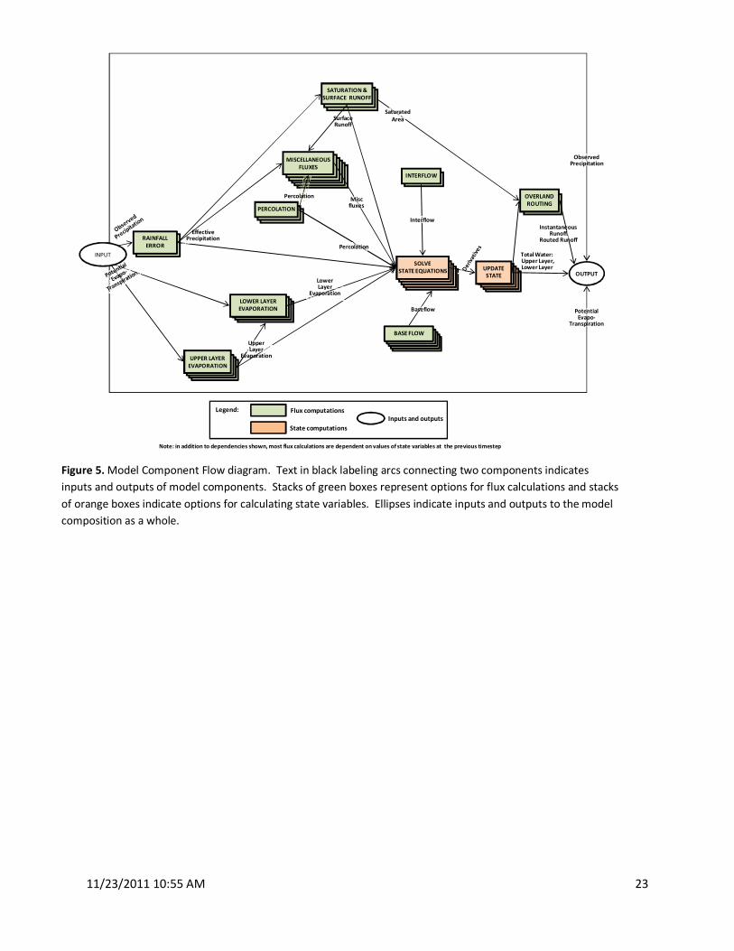
Figure 5 contains a high-level view of the flow of data at execution among these components. The
MARIO FUSE components are depicted as stacks of components, each representing the variant used for
a specific model configuration option as described in Table 1, second column. When a user conveys a
model configuration to MARIO, MARIO assembles at most one component from each stack, linking
outputs of some to inputs of others. Thus, each configured model consists only of the formulae needed
for that model, eliminating the need for runtime decision logic.
As mentioned above, FUSE’s core flux calculations are controlled by collections of many FORTRAN CASE
statements and FOR loops. When a new soil architecture, flux computation, or other modeling
characteristic is added, changes must be made throughout the FORTRAN code, increasing code
complexity and the likelihood of incorrect operation. Converting these modules to composable
components and relying on MARIO’s rigorous application of composition rules, all possible model
compositions are explored, guided by simple expressions of flux dependencies, preventing the creation
of Frankenmodels.
Semantic Tagging of FUSE components
To enable automated model composition, each component is annotated with tags, light-weight
semantic descriptions of the component’s inputs, outputs, and configuration parameters, as shown in
Figure 7 and described in an earlier section (MARIO: A New Approach to Model Integration).
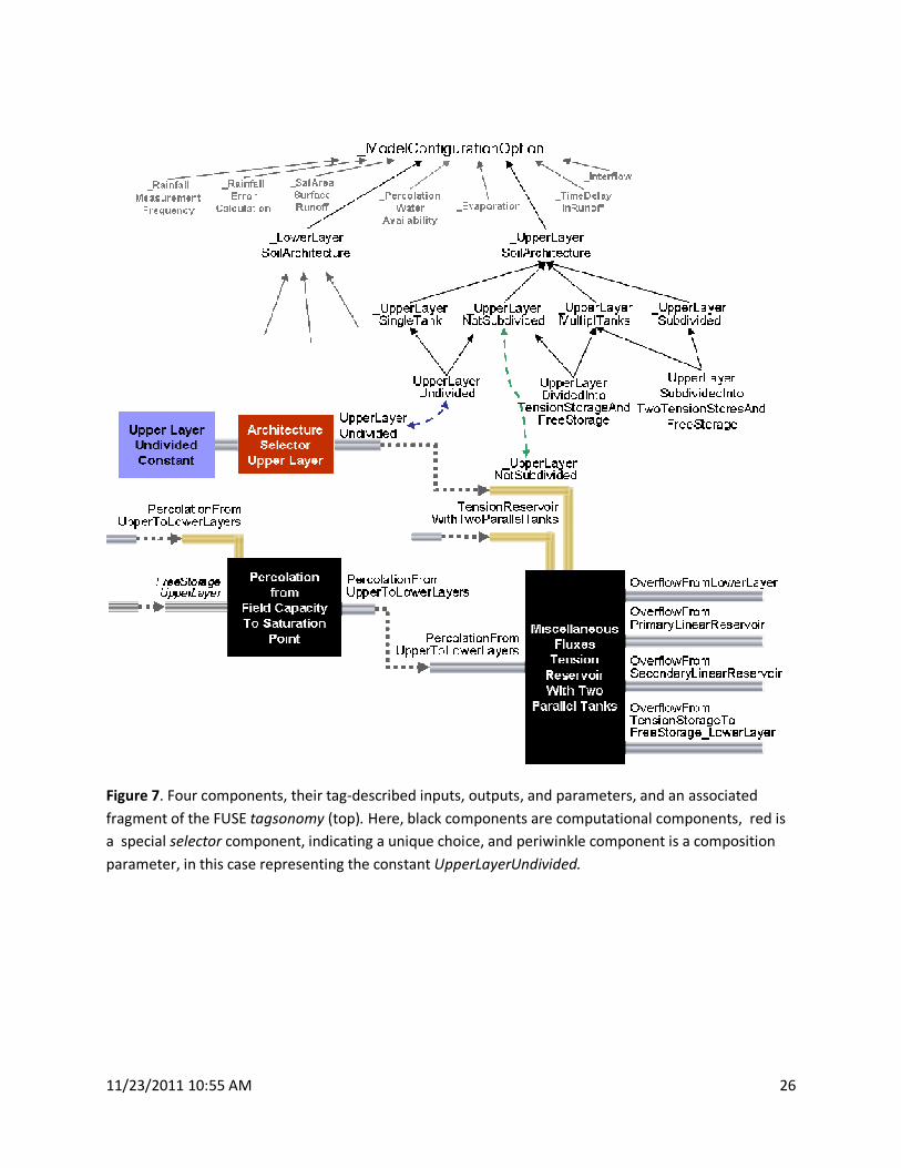
Figure 7 (top) includes a fragment of this application’s tagsonomy, beginning at the top with tags
corresponding to the 9 top-level model configuration options (e.g., RainfallMeasurementFrequency).
The descendant tags extending UpperLayerSoilArchitecture represent the various upper layer
architecture choices shown in Figure 3; for example, the
UpperLayerDividedIntoTensionStorageAndFreeStorage tag reflects the Sacramento architecture, while
UpperLayerUndivided a reflects an architecture shared by TOPMODEL and ARNO/VIC.
11/23/2011 10:55 AM 11
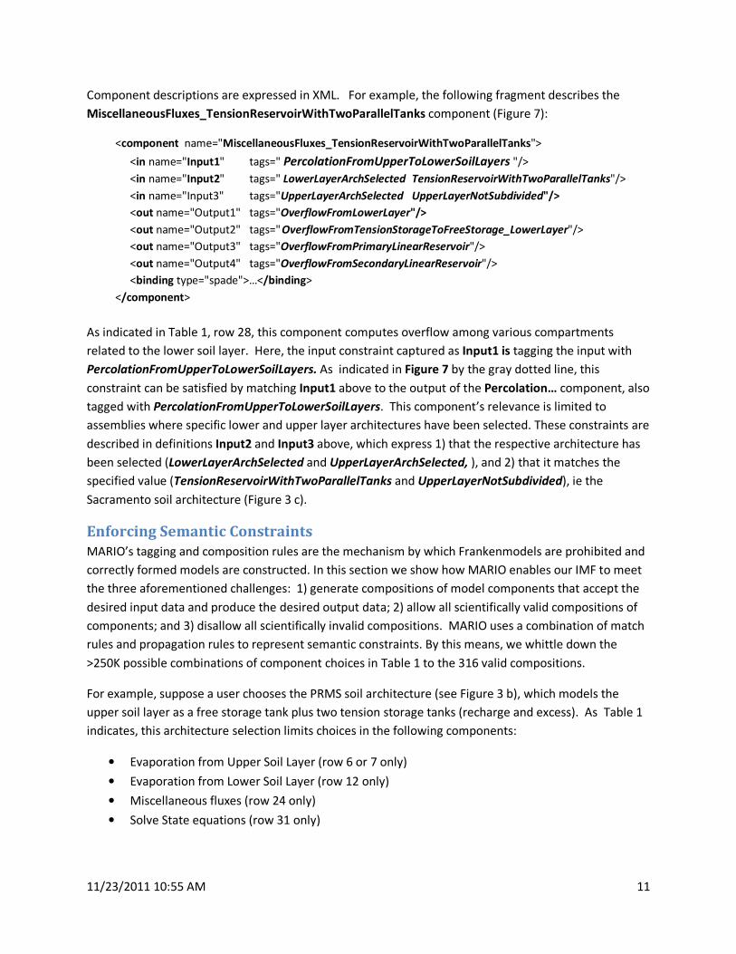
Component descriptions are expressed in XML. For example, the following fragment describes the
MiscellaneousFluxes_TensionReservoirWithTwoParallelTanks component (Figure 7):
<component name="MiscellaneousFluxes_TensionReservoirWithTwoParallelTanks">
<in name="Input1" tags=" PercolationFromUpperToLowerSoilLayers "/>
<in name="Input2" tags=" LowerLayerArchSelected TensionReservoirWithTwoParallelTanks"/>
<in name="Input3" tags="UpperLayerArchSelected UpperLayerNotSubdivided"/>
<out name="Output1" tags="OverflowFromLowerLayer"/>
<out name="Output2" tags=" OverflowFromTensionStorageToFreeStorage_LowerLayer"/>
<out name="Output3" tags="OverflowFromPrimaryLinearReservoir"/>
<out name="Output4" tags="OverflowFromSecondaryLinearReservoir"/>
<binding type="spade">…</binding>
</component>
As indicated in Table 1, row 28, this component computes overflow among various compartments
related to the lower soil layer. Here, the input constraint captured as Input1 is tagging the input with
PercolationFromUpperToLowerSoilLayers. As indicated in Figure 7 by the gray dotted line, this
constraint can be satisfied by matching Input1 above to the output of the Percolation… component, also
tagged with PercolationFromUpperToLowerSoilLayers. This component’s relevance is limited to
assemblies where specific lower and upper layer architectures have been selected. These constraints are
described in definitions Input2 and Input3 above, which express 1) that the respective architecture has
been selected (LowerLayerArchSelected and UpperLayerArchSelected, ), and 2) that it matches the
specified value (TensionReservoirWithTwoParallelTanks and UpperLayerNotSubdivided), ie the
Sacramento soil architecture (Figure 3 c).
Enforcing Semantic Constraints
MARIO’s tagging and composition rules are the mechanism by which Frankenmodels are prohibited and
correctly formed models are constructed. In this section we show how MARIO enables our IMF to meet
the three aforementioned challenges: 1) generate compositions of model components that accept the
desired input data and produce the desired output data; 2) allow all scientifically valid compositions of
components; and 3) disallow all scientifically invalid compositions. MARIO uses a combination of match
rules and propagation rules to represent semantic constraints. By this means, we whittle down the
>250K possible combinations of component choices in Table 1 to the 316 valid compositions.
For example, suppose a user chooses the PRMS soil architecture (see Figure 3 b), which models the
upper soil layer as a free storage tank plus two tension storage tanks (recharge and excess). As Table 1
indicates, this architecture selection limits choices in the following components:
• Evaporation from Upper Soil Layer (row 6 or 7 only)
• Evaporation from Lower Soil Layer (row 12 only)
• Miscellaneous fluxes (row 24 only)
• Solve State equations (row 31 only)
11/23/2011 10:55 AM 12
MARIO ensures that these components and only these components are selected, given the architecture
choice, by associating the tag UpperLayerSubdivided and its children exclusively to them.
Not evident in Table 1 is a more subtle constraint, represented in FUSE by a FORTRAN if-statement: “do
not allow percolation below field capacity if the upper soil layer has multiple tension storage tanks”,
namely, the excess and recharge zones. Therefore the choice of PRMS upper soil architecture limits the
choice of percolation components to choices 2 and 3. As introduced earlier, parent tags were used in
MARIO to express this constraint. For this case, UpperLayerUndivided, a specific type of
UpperLayerSoilArchitecture, was classified as being an UpperLayerArchitectureSingleTank. All other
upper layer architectures were classified as UpperLayerArchitectureMultipleTanks. To enforce the
above constraint on percolation, we explicitly restricted the Percolation_WiltPointToSat component to
be assembled only when the upper layer architecture is one of the children of
UpperLayerArchitectureSingleTank. Note that UpperLayerUndivided is currently the only upper layer
architecture defined as UpperLayerArchitectureSingleTank; if a new kind of upper architecture were to
be introduced and classified as a single tank architecture, it would automatically be allowed in the
assembly with Percolation_WiltPointToSat, with all other combinations still being excluded. This occurs
without any additional procedural programming, and without recompilation and/or reinstallation of
MARIO.
Results
The culmination of our current work is an interface whereby hydrologist users can interact with MARIO,
select among model composition options, examine the resultant assembled flows, refine goals, etc., and
where component developers can insert additional components for immediate inclusion in subsequent
user requests. When our work is complete (with component descriptions bound to real, running code in
FORTRAN, SPADE , C++, etc.), those users could, at any time, submit any assembled flow for deployment
and operation and can view result data via a variety of data visualizers.
As currently configured, users can interact with MARIO to do two main things: 1) guide MARIO to
construct any of a large number of scientifically valid model compositions by selecting among the FUSE
model configuration options, and 2) browse and select combinations of the many available flux and
state computations and apply these “sub-models” to precipitation data for visualization and exploration.
Since MARIO applies its composition rules to the component semantic descriptions, any selectable
combination of tags – complete water models or finer grained flux calculation sub-models – is a valid
and deployable composition, assuming that the developer has correctly crafted both the component
descriptions and the associated computation code.
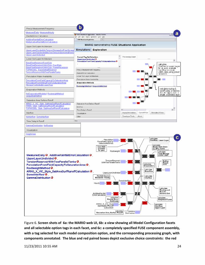
A hydrologist’s first view of MARIO for FUSE can be seen in Figure 6a. Here, the user can 1) have MARIO
construct total water analysis models (under the Simulations tab) or 2) select among the various fluxes
and calculations (under the Exploration tab).
Model configuration options for Simulations, reflected in Figure 6b, are grouped into facets,
corresponding to the Calculation column of Table 1. Figure 6a (right) shows the top-ranked composition
11/23/2011 10:55 AM 13
graph produced when two configuration options have been selected ( UpperLayerUndivided for the
Upper Soil Layer Architecture and PercolationFromFieldCapacityToSaturationArea for the Percolation
Water Availability facet). Note that MARIO has automatically assembled a complete, ready-to-deploy
simulation, selecting options for each as-yet unspecified category.6 The user can deploy this simulation
or can continue to refine the goal.
Figure 6c shows the fully elaborated, user-selected goal consisting of one option from each category
(left), and the corresponding flow composition assembled for that goal (right). The flow diagram has
been annotated to describe each computational component. The description of each has been
abbreviated. It is possible to identify which of the 39 flux computation components has been selected by
its name, in combination with the model decisions, which are represented in the paired blue and red
components. For example, the component for calculation of Saturation and Surface Runoff would be
component 3 (Table 1), because the selected method is
ARNO_X_VICStyle_SatAreaSurfaceRunoffCalculation.
As mentioned above, the initial set of model elements and computational components can be extended.
As component developers identify new soil architectures and/or new ways to calculate fluxes, they
register these new elements with MARIO; hydrologists can employ the new options and components
immediately. Other analytic toolkits can be incorporated, including those available with InfoSphere
Streams, to apply, e.g., comparative analytics to collections of models. Also, additional data sources can
be added, such as web-accessible datasets and even live streaming water sensors. Given a scalable
model runtime environment such as InfoSphere Streams, many analyses across multiple, high volume
data sources provide an environment for high performance water data analysis and exploration.
Discussion
In this paper we have shown how the semantic tagging and model composition engine of the MARIO
project enable us to meet three critical challenges of an IMF: 1) generating valid chain(s) or
compositions of model components, given a definition of starting and ending states ; 2) allowing all
scientifically valid compositions of components; and 3) disallowing compositions that are scientifically
invalid, i.e., that combine model components whose basic assumptions about quantities like soil
architectures or evaporation schemes conflict. The advantages of this system when compared to other
model framework systems mentioned in the Motivation section are many. A declarative approach to
constraint specification frees users from the error-prone and tedious practice of manually programming
constraints in FORTRAN via nested loops and CASE statements. The tagsonomy allows the expression
and enforcement of constraints that are higher level than simple type-checking of inputs and outputs of
model components. Since constraint specification is declarative, it is relatively easy to extend the
system with new components written (or wrappered) to the MARIO/SPADE interface specification—
whether components that compute the same fluxes in a new way, or components that compute new
6 The complete graph was generated to satisfy _FullModelResultSet, and implicit goal element for Simulations.
This tag represents the generation of all result data output by each FUSE simulation.
11/23/2011 10:55 AM 14
fluxes. MARIO’s flow generation and automatic composition enable multiple different compositions of a
set of components to be generated and run---invaluable in a multi-model, ensemble-based modeling
approach. Unlike the case of models written as monolithic FORTRAN programs, MARIO’s handling
computation at the component level allows the investigation of intermediate results at any stage along
the model composition flow.
There is nonetheless further work to be done before we can demonstrate a fully functional IMF. In this
paper we focused on componentization of models, and the representation and management of
metadata expressing their semantics. An obvious next step is to associate these conceptual components
to executable code, either in FORTRAN for complex computations such as the solution of the differential
state equations, or in the SPADE language for the relatively simple algebraic expressions used in many of
the FUSE flux calculations. The components will then be candidates for parallel execution in InfoSphere
Streams, which could dramatically increase performance, especially in multi-model, ensemble-based
methods, or when exploring large parameter spaces in autocalibration/parameter estimation. The
stream-based data model of InfoSphere Streams will also facilitate connecting the system to real-time or
near-real-time streaming sensor data, such as precipitation data.
Incorporating visualization tools will allow the rich and complex data sets that are produced in the
stream discharge simulator to be effectively conveyed and will enable non-expert users to make full use
of the relevant features of the framework. The MARIO interface will make this task particularly easy,
since 1) the results of any calculation would be available for presentation to the user, and 2) the user
need only select the tags corresponding to the desired data to see the data.
In our further work with this system, we plan to carry out several explorations of extensibility, for
example:
• componentizing and incorporating another monolithic model, e.g., the USGS’s Hydrological
Simulation Program—FORTRAN (HSPF) [14]
• integrating simulations of stream discharges from multiple watersheds to determine stream
discharges in a river network
• include more hydrologic processes in the stream discharge simulators such as infiltration-
excess runoff and processes representing role of vegetation in the hydrologic cycle, such as
the effect of vegetation canopy on the magnitude and rate of precipitation delivered to the
soil surface
• integrating an explicit groundwater model to simulate coupled surface-groundwater systems,
to allow users to simultaneously manage surface and groundwater resources
Conclusion
In this paper we have broken new ground in the development of the Integrated Modeling Framework
that is needed in many disciplines and domains related to the Intelligent Infrastructure. We have
described a research prototype that supports: registering model components in a specific domain;
expressing the semantics of the model components in a standardized set of metadata; expressing and
enforcing rich, domain-specific semantic constraints on how model components may be validly
11/23/2011 10:55 AM 15
composed together and assembled to form larger simulations; and generating valid component
assemblies, and excluding assemblies which violate the expressed domain-specific semantic constraints,
thus avoiding Frankenmodels, model assemblies that execute but are scientifically invalid. We have
demonstrated this work using the complex, real-world example of the calculation of stream discharge
from observed precipitation, building on the foundation of real-world FORTRAN modules. The use of
this example has challenged and stretched IBM’s MARIO research technology, and in the process
demonstrated its great utility. Once model developers have registered the model components and
their semantics with MARIO, component assemblies may be built by non-expert modelers with the
assurance that the model semantics will not be violated, and therefore only scientifically valid
assemblies will be generated and run. While we have focused on a single complex but fairly narrow
application domain (stream discharge in hydrology), we fully expect that our approach will be readily
applicable to a wide variety of related domains (e.g., water quality, carbon balance, crop production,
and biodiversity), and to other domains that are critical for intelligent water management, e.g.,
demographics, financials, weather, geographic information systems, and real-time streaming data from
such devices as water meters, water quality sensors, and fault-detection devices in smart levees. From
here it is not unreasonable to imagine applications to cities, transportation, utilities, and other key areas
making up our vision of the Intelligent Infrastructure.
References
See end of paper after tables and figures.
Acknowledgments
The authors extend warm thanks to Martyn Clark of the National Institute of Water and Atmospheric
Research (NIWA) in Christchurch, New Zealand, for generously allowing us to build upon his FUSE code
and answering our questions about it. We thank Steve De Gennaro, Ron Ambrosio, and Jeff Katz of IBM
for discussions of solution architectures for the Smarter Planet initiative. We also thank Anand
Ranganathan and others who worked on MARIO at IBM: Eric Bouillet, Hanhua Feng, Zhen Liu and
Octavian Udrea. This work would not be possible without them. Finally, we thank Peter Williams of
IBM’s Big Green Innovations group, for his helpful suggestions and for introducing Alex Mayer to the rest
of the co-authors (a match made in a place very near to heaven).
11/23/2011 10:55 AM 16
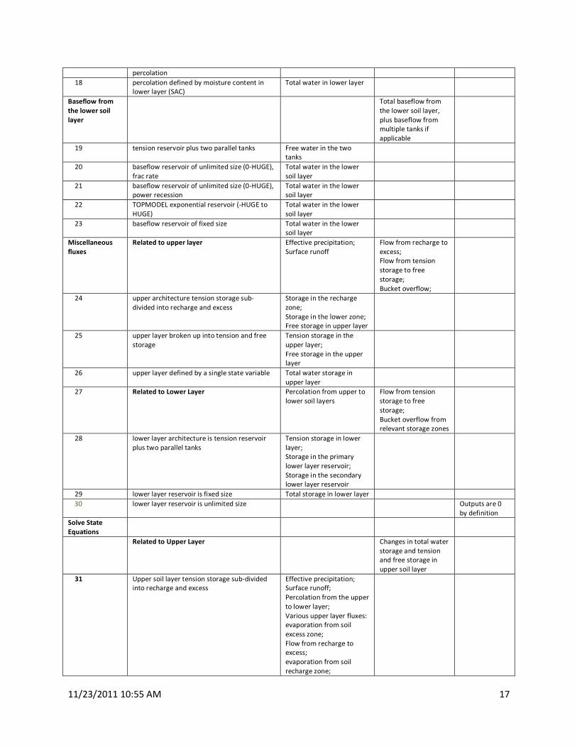
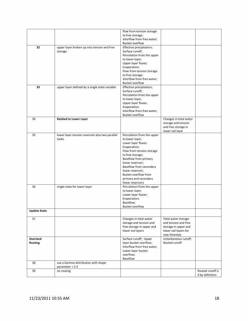
Table 1. Description of flux and state calculations in FUSE, represented as individual model components in
MARIO. Inputs and outputs that are the same for all options are listed on the row which specifies the
calculation. Inputs and comments that differ by option are listed on the row which specifies the option.
Calculation Model options Inputs Outputs Comments
Rainfall Error Observed precipitation Effective precipitation
1 Additive error correction No additional
inputs
2 Multiplicative error correction No additional
inputs
Saturation and
Surface Runoff
Effective precipitation Saturated area
Surface runoff
3 ARNO Xhang VIC Upper level water
4 PRMS Variant Upper level tension store
5 TOPMODEL Parameterization Lower level water
Evaporation
from Upper Soil
Layer
Potential
evapotranspiration
Total Evaporation,
plus evaporation
from from 2 separate
upper layer soil
compartments
If upper soil
architecture
doesn’t support
multiple
compartments,
values set to 0
6 Tension storage sub-divided into recharge and
excess; sequential evaporation scheme
Tension storage in
recharge and excess tanks
7 Tension storage sub-divided into recharge and
excess; rootweight evaporation scheme
Tension storage in
recharge and excess tanks
8 Single tension store + free store or one state;
sequential evaporation
Tension storage
9 Single tension store + free store or one state;
rootweight evaporation
Tension storage
Evaporation
from Lower Soil
Layer
Potential
evapotranspiration
Evaporation from the
lower soil layer
10 Lower layer architecture is either fixed size or
a tension reservoir plus two parallel tanks;
Upper layer architecture is either single
tension store+ free store or one state;
sequential lower-layer evaporation scheme
Tension storage in lower
soil layer
11 Lower layer architecture is either fixed size or
a tension reservoir plus two parallel tanks;
Upper layer architecture is either single
tension store + free store or one state;
rootweight lower-layer evaporation scheme
Tension storage in lower
soil layer
12 Lower layer architecture is either fixed size or
a tension reservoir plus two parallel tanks;
Upper layer tension storage is sub-divided
into recharge and excess;
Evaporation
from the lower
layer is 0 by
definition
13 Lower layer architecture is either baseflow
reservoir of unlimited size (0-HUGE) with a
fractional rate, or baseflow reservoir of
unlimited size (0-HUGE) with a power
recession, or TOPMODEL exponential
reservoir (-HUGE to HUGE)
Evaporation
from the lower
layer is 0 by
definition
Interflow Interflow from free
water in upper layer
14 Some interflow Free water in upper layer
15 No interflow Interflow = 0 by
definition
Percolation from
upper to lower
soil layers
Percolation from
upper to lower soil
layers
16 water from (field capacity to saturation) avail
for percolation
Free water in upper layer
17 water from (wilt point to saturation) avail for Total water in upper layer
11/23/2011 10:55 AM 17
percolation
18 percolation defined by moisture content in
lower layer (SAC)
Total water in lower layer
Baseflow from
the lower soil
layer
Total baseflow from
the lower soil layer,
plus baseflow from
multiple tanks if
applicable
19 tension reservoir plus two parallel tanks Free water in the two
tanks
20 baseflow reservoir of unlimited size (0-HUGE),
frac rate
Total water in the lower
soil layer
21 baseflow reservoir of unlimited size (0-HUGE),
power recession
Total water in the lower
soil layer
22 TOPMODEL exponential reservoir (-HUGE to
HUGE)
Total water in the lower
soil layer
23 baseflow reservoir of fixed size Total water in the lower
soil layer
Miscellaneous
fluxes
Related to upper layer Effective precipitation;
Surface runoff
Flow from recharge to
excess;
Flow from tension
storage to free
storage;
Bucket overflow;
24 upper architecture tension storage sub-
divided into recharge and excess
Storage in the recharge
zone;
Storage in the lower zone;
Free storage in upper layer
25 upper layer broken up into tension and free
storage
Tension storage in the
upper layer;
Free storage in the upper
layer
26 upper layer defined by a single state variable Total water storage in
upper layer
27 Related to Lower Layer Percolation from upper to
lower soil layers
Flow from tension
storage to free
storage;
Bucket overflow from
relevant storage zones
28 lower layer architecture is tension reservoir
plus two parallel tanks
Tension storage in lower
layer;
Storage in the primary
lower layer reservoir;
Storage in the secondary
lower layer reservoir
29 lower layer reservoir is fixed size Total storage in lower layer
30 lower layer reservoir is unlimited size Outputs are 0
by definition
Solve State
Equations
Related to Upper Layer Changes in total water
storage and tension
and free storage in
upper soil layer
31 Upper soil layer tension storage sub-divided
into recharge and excess
Effective precipitation;
Surface runoff;
Percolation from the upper
to lower layer;
Various upper layer fluxes:
evaporation from soil
excess zone;
Flow from recharge to
excess;
evaporation from soil
recharge zone;
11/23/2011 10:55 AM 18
flow from tension storage
to free storage;
Interflow from free water;
Bucket overflow
32 upper layer broken up into tension and free
storage
Effective precipitation;
Surface runoff;
Percolation from the upper
to lower layer;
Upper layer fluxes:
Evaporation;
Flow from tension storage
to free storage;
Interflow from free water;
Bucket overflow
33 upper layer defined by a single state variable
Effective precipitation;
Surface runoff;
Percolation from the upper
to lower layer;
Upper layer fluxes:
Evaporation;
Interflow from free water;
Bucket overflow
34 Related to Lower Layer Changes in total water
storage and tension
and free storage in
lower soil layer
35 lower layer tension reservoir plus two parallel
tanks
Percolation from the upper
to lower layer;
Lower layer fluxes:
Evaporation;
Flow from tension storage
to free storage;
Baseflow from primary
linear reservoir;
Baseflow from secondary
linear reservoir;
Bucket overflow from
primary and secondary
linear reservoirs
36 single state for lower layer
Percolation from the upper
to lower layer;
Lower layer fluxes:
Evaporation;
Baseflow;
Bucket overflow
Update State
37 Changes in total water
storage and tension and
free storage in upper and
lower soil layers
Total water storage
and tension and free
storage in upper and
lower soil layers for
new timestep
Overland
Routing
Surface runoff; Upper
layer bucket overflow;
Interflow from free water;
Lower layer bucket
overflow;
Baseflow
instantaneous runoff;
Routed runoff
38 use a Gamma distribution with shape
parameter = 2.5
39 no routing Routed runoff is
0 by definition
11/23/2011 10:55 AM 19
Figure 1. Intelligent Infrastructure Reference Architecture. The Service-Oriented Architectural foundation of the Intelligent
Infrastructure, integrating (near-) real-time sensor data, analytics, and controls with enterprise data, applications, analytics,
modeling/simulation, and user interfaces/visualization. The orange box in the upper right highlights the portion of the
architecture that this paper addresses.
Key to abbreviations: ETL= Extract, Transform, Load data warehousing services. GIS = Geographic Information Systems.
SCADA=Supervisory Control and Data Acquisition. MES=Manufacturing Execution System. ERP=Enterprise Resource
Planning.
ES
BUser
Interfaces
Analytics Device Control/
Monitoring
Related data
ETL service
Simulation Manager
Model Component
Manager
Visualization
Data Transformation
Rules Manager
Business
Applications
Data Historian
Demographics
GIS
Environment
Weather
Local Connections (Ethernet, SCADA, Internal Buses)
Operational
Logic
Cameras,
webcams
Intelligent
sensors
Process/Workflow
Choreography
Device controllers
(pumps, switches…)
Time-Dependent Middleware
MES,
Process
Control
Meters
Enterprise Service Bus (ESB)
High-performance Analytics
Computation Engine
Network device
monitoring and control
(eg SCADA)
Event
DetectionLocal
AnalyticsOperational
Monitoring
Complex
Event Processing
Modeling
In situ
sensorsRemote
sensors
�Analytics Engine
�Geo-spatial Data
Mining
�Statistics
�Risk Assessment
�SCADA
�MES
�ERP
�Asset
Management
�Scheduling/
Forecasting
�Inputs
�Outputs
�Administration
Collaboration
�Reporting
�Dashboard
�Email/pager
Data
Warehouse
�Analytics Rule
Base
�Rules Engine
�Alerts
�Access Mgrs
�Remote config
and management
�Complex event
processing
High-performance archiving
of time-series data
MARIO
11/23/2011 10:55 AM 20
wind
groundwater
storage
precipitation
tra
nsp
ira
tio
n
ev
ap
ora
tio
n
ev
ap
ora
tio
n
interception
storage
snow
runoff
infi
ltra
tio
n
rech
arg
e
refl
ect
ed
an
d
lon
gw
av
e r
ad
iati
on
refl
ect
ed
an
d
lon
gw
av
e r
ad
iati
on
shortwave
radiation
baseflow
soil moisture
storage
Figure 2. Illustration of hydrologic cycle, including water storage compartments and pathways for water
movement in the atmosphere and over and through the land surface (fluxes). Components of energy fluxes that
drive the hydrologic cycle also are depicted.
11/23/2011 10:55 AM 21
upper soil
zone evapotranspiration
lower soil
zone
qsx
, qif 1
Sd
dt
Δ storage
runoff
qb
e1
precipitation
p
e2 q
12
2Sd
dt
(a) GENERIC
(b) PRMS (c) SACRAMENTO
(d) TOPMODEL (e) ARNO/VIC
Figure 3. Schematic representations of two-zone systems: (a) generic system with terms for changes in water storage for each zone
and corresponding water fluxes; (b) – (e) parent model modular systems, indicating differences among models in terms of fluxes
and sub-divisions of zone storages and fluxes. S is storage in each soil zone; e is evapotranspiration from each soil zone; p is
precipitation; q12 is percolation; qsx is saturation-excess runoff; qif is interflow (lateral flux through the upper layer to the stream); qb
is baseflow (lateral fluxes through the lower layer to the stream ); Zuz and Zlz are depths of the upper and lower soil layers,
respectively; θwlt, θfld, and θsat are soil moistures at wilting point, field capacity, and saturation, respectively; indices 1 and 2 denote
the upper and lower soil zones, respectively; indices T and F denote stored water held in tension (retained by capillary forces) and
freely-flowing water in storage; and indices A and B denote further sub-divisions of soil zones.
11/23/2011 10:55 AM 22
Figure 4. The MARIO cross-platform architecture with example data sources and processing components from
the financial domain.
11/23/2011 10:55 AM 23
RAINFALL
ERROR
RAINFALL
ERROR
SATURATION &
SURFACE Runoff
OVERLAND
ROUTING
UPDATE
STATE
UPDATE
STATE
UPDATE
STATE
UPDATE
STATESOLVE
STATE EQUATIONS
SOLVE
STATE EQUATIONS
SOLVE
STATE EQUATIONS
SOLVE
STATE EQUATIONS
PERCOLATIONPERCOLATION
MISCELLANEOUS
FLUXES
MISCELLANEOUS
FLUXES
MISCELLANEOUS
FLUXES
MISCELLANEOUS
FLUXES
MISCELLANEOUS
FLUXES
UPPER LAYER
EVAPORATION
UPPER LAYER
EVAPORATION
UPPER LAYER
EVAPORATION
LOWER Layer EVAPORATION
LOWER Layer
EVAPORATION
LOWER Layer
EVAPORATION
INTERFLOW
BASE FLOWBASE FLOWBASE FLOW
SATURATION &
SURFACERunoff
PERCOLATION
INTERFLOW
SOLVE
STATE EQUATIONS
LOWER LAYER
EVAPORATION
UPPER LAYER
EVAPORATION
Miscfluxes
UPDATE
STATE
Note: in addition to dependencies shown, most flux calculations are dependent on values of state variables at the previous timestep
Instantaneous Runoff
Routed Runoff
Total Water:Upper Layer, Lower Layer
OUTPUT
Legend: Flux computations
State computations
Inputs and outputs
SATURATION &
SURFACE RUNOFF
Upper Layer
Evaporation
Lower Layer
Evaporation
EffectivePrecipitation
BASE FLOWBASE FLOW
OVERLAND
ROUTING
Interflow
Baseflow
Saturated
AreaSurface Runoff
Observed Precipitation
Potential Evapo-
Transpiration
Percolation
MISCELLANEOUS
FLUXES
Percolation
INPUT
Figure 5. Model Component Flow diagram. Text in black labeling arcs connecting two components indicates
inputs and outputs of model components. Stacks of green boxes represent options for flux calculations and stacks
of orange boxes indicate options for calculating state variables. Ellipses indicate inputs and outputs to the model
composition as a whole.
11/23/2011 10:55 AM 24
Figure 6. Screen shots of 6a: the MARIO web UI, 6b: a view showing all Model Configuration facets
and all selectable option tags in each facet, and 6c: a completely specified FUSE component assembly,
with a tag selected for each model composition option, and the corresponding processing graph, with
components annotated. The blue and red paired boxes depict exclusive choice constraints: the red

11/23/2011 10:55 AM 25
box is a singleton selector, allowing exactly one value of the respective model configuration option.
Without such a constraint, any component calling for, e.g., and upper layer architecture choice could
be satisfied by any of the upper layer architecture options.
11/23/2011 10:55 AM 26
Figure 7. Four components, their tag-described inputs, outputs, and parameters, and an associated
fragment of the FUSE tagsonomy (top). Here, black components are computational components, red is
a special selector component, indicating a unique choice, and periwinkle component is a composition
parameter, in this case representing the constant UpperLayerUndivided.
11/23/2011 10:55 AM 27
References
[1] C. Harrison, B. Eckman, R. Hamilton, P. Hartswick, J. Kalagnanam, J. Paraszczak, and P. Williams,
"Foundations for Smart Cities," IBM Journal of Research & Development, Special Issue on
Supporting a 'Smarter Planet' with Technology, (2010).
[2] B. Eckman, C. Barford, P. West, and G. Raber, "Intuitive simulation, querying, and visualization for
river basin policy & management," IBM Journal of Research & Development, Special Issue on
Technologies for Environmental Stewardship, (2009).
[3] M. Kehoe, E. Alvey, H. Badawi, B. Brech, S. DeGennaro, R. DeMaine, P. Hartswick, A. Heys, J. Hogan,
J. Katz, and D. Waxman, "Smart Cities Solution Architectures: A RedGuide for Business Leaders,"
2009.
[4] M. Clark, A. Slater, D. Rupp, R. Woods, J. Vrugt, H. Gupta, T. Wagener, and L. Hay, "Framework for
Understanding Structural Errors (FUSE): A modular framework to diagnose differences between
hydrological models," Water Resources Research, vol. 44, p. W00B02 (2008).
[5] G Leavesley, P Restrepo, S Markstrom, M Dixon, and L Stannard, The Modular Modeling System
(MMS): User's Manual, U.S. Geological Survey, Denver, CO,1996.
[6] J Gregersen, P Gijsbers, and S Westen, "OpenMI : Open Modelling Interface," Journal of
Hydroinformatics, pp. 175-191 (2007).
[7] Consortium of Universities for the Advancement of Hydrologic Science Inc, "Community Hydrologic
Modeling Platform (CHyMP)," 2009. http://www.cuahsi.org/chymp.html
[8] A. V. Riabov, E. Bouillet, M. D. Feblowitz, Z. Liu, and A. Ranganathan, "Wishful Search: Interactive
Composition of Data Mashups," World Wide Web Conference (WWW-08), Beijing, China, Apr 21-
25, 2008., (2008).
[9] E. Bouillet, M. D. Feblowitz, H. Feng, Z. Liu, A. Ranganathan, A. V. Riabov, and O. Udrea, "MARIO:
Middleware for Assembly and Deployment of Complex Multi-platform Applications,"
ACM/IFIP/USENIX 10th International Middleware Conference, Urbana Champaign, Illinois, USA,
November 30 - December 4, 2009, (2009).
[10] E. Bouillet, M. D. Feblowitz, Z. Liu, A. Ranganathan, and A. V. Riabov, "Semantic Matching,
Propagation and Transformation for Composition in Component-Based Systems," International
Journal of Software Science and Computational Intelligence (IJSSCI), vol. 1, No. 1 (2009).
[11] "Delicious," 2009. http://delicious.com
[12] IBM, "InfoSphere Streams," 2009. http://www.ibm.com/software/data/infosphere/streams/
[13] B. Gedik, H. Andrade, K.-L. Wu, P. S. Yu, and M. Doo, "SPADE: The System S Declarative Stream
Processing Engine. " International Conference on Management of Data, ACM SIGMOD, (2008).

11/23/2011 10:55 AM 28
[14] B. Bicknell, J. Imhoff, J. Kittle, Jr. A. Donigian, and R. Johanson, Hydrological Simulation Program--
Fortran, User's manual for version 11, U.S. Environmental Protection Agency, National Exposure
Research Laboratory, Athens, Ga,1997.