Zhang Y., Li G., Muskat B., Law R. (2020). Tourism Demand Forecasting: A Decomposed Deep Learning Approach, Journal of Travel Research. doi: 10.1177/0047287520919522

https://journals.sagepub.com/doi/full/10.1177/0047287520919522

Tourism Demand Forecasting: A Decomposed Deep Learning Approach

ABSTRACT

Tourism planners rely on accurate demand forecasting. However, despite numerous advancements, crucial methodological issues remain unaddressed. This study aims to further improve the modeling accuracy and advance the artificial intelligence (AI)-based tourism demand forecasting methods. Deep learning models that predict tourism demand are often highly complex and encounter overfitting, which is mainly caused by two underlying problems: 1) access to limited data volumes and 2) additional explanatory variable requirement. To address these issues, we use a decomposition method that achieves high accuracy in short- and long-term AI-based forecasting models. The proposed method effectively decomposes the data and increases accuracy without additional data requirement. In conclusion, this study alleviates the overfitting issue and provides a methodological contribution by proposing a highly accurate deep learning method for AI-based tourism demand modeling.

Keywords

Tourism demand forecasting, tourism planning, AI-based forecasting, deep learning, decomposing method, overfitting

1 INTRODUCTION

Tourism planners require accurate forecasting of tourist arrival data (Law, Li, Fong, & Han,

2019; Li & Law, 2020; Wan & Song, 2018). Similarly, destinations and all actors within the

tourism value chain, such as the transportation sector, tour operators, accommodation

providers, event organizers, and retailers, require accurate forecasts to make short-term

decisions that meet their operational demands, as well as to develop long-term strategies to

analyze market trends, set priorities, and manage risks. Given such importance, tourism

demand forecasting retains high research interest (Law et al., 2019; Sun, Wei, Tsui, & Wang,

2019; Wan & Song, 2018).

Despite numerous advancements in the three modeling categories of tourism

forecasting literature (i.e., time series, econometric, and artificial intelligence [AI]), several

crucial methodological problems still require further attention (Chen, Li, Wu, & Shen, 2019;

Li & Law, 2020; Wan & Song, 2018). Highly sophisticated modeling approaches are used to

address these methodological challenges, including econometric Bayesian vector

autoregressive (BVAR) models, market interpretation/data analysis system (Assaf, Li, Song,

& Tsionas, 2019; Bangwayo-Skeete & Skeete, 2015), and advanced AI-based models, such as

deep learning (DL) (Law et al., 2019).

This study applies AI-based techniques to improve the accuracy of tourism demand

forecasting modeling; techniques include traditional machine learning algorithms (Sun et al.,

2019) and advanced DL methods (Law et al., 2019; LeCun, Bengio, & Hinton, 2015; Ma,

Xiang, Du & Fan, 2018). The latter have powerful feature engineering and can automatically

extract relevant demand indicators (Law et al., 2019). Despite the advantages of AI-based

methods, two major problems cause overfitting of the predictive model. The first problem is

the limited data volume. For example, time series data might only capture 5–10 years’ worth

of data or even merely 60–200 samples (Frechtling, 2012). Limited data volume can lead to

underperformance in future actual testing data, despite a close fit in the training data (Hawkins,

2004, Wang et al., 2013) in traditional and AI-based models.

The second problem is rooted in the necessity to add extra variables. To increase

accuracy, existing AI-based tourism demand forecasting studies commonly incorporate

additional explanatory variables (Law et al., 2019; Yang, Pan, & Song, 2014). However, such

additions are problematic due to possible variable redundancy and lead to overfitting (Pan, Liu,

& Huang, 2017; Niu et al., 2011). In addition, explanatory variables often require further

processing, such as filtering the unimportant items or selecting the most important ones. This

process is referred to as feature engineering (Zheng & Casari, 2018), which can only be handled

with highly specialized expertise. Law et al. (2019) suggested using a single attention

mechanism for automatic feature engineering and lag order selection instead of manual

processing. However, the proposed dynamic linear modeling (DLM) is unreliable in identifying

relevant variables and their lags, especially when the available data is insufficient (Law et al.,

2019).

To address these problems, the present study applies the recent DL approach to tourism

demand forecasting. We use a decomposition method to increase the accuracy of short- and

long-term AI-based forecasting models, and to effectively decompose the data (Li & Law, 2020;

Silva et al., 2019). Using this decomposition approach, we develop an AI-based forecasting

model that can achieve high accuracy without additional data requirement. Decomposition

methods divide the initial dataset into smaller stationary sub-series, a process labelled divide-

and-conquer (Qiu, Ren, Sungathan, & Amaratunga, 2017). These stationary sub-series can be

forecasted separately without further requirements, and thus effectively utilize the available

data.

The methodological contributions of this research are twofold. First, we address the

overfitting issue caused by limited data volume, especially in highly complex models through

the seasonal and trend decomposition using Loess (STL), which generates a relatively simple

forecasting process. Second, we propose a novel deep learning approach and use a duo attention

deep learning model (DADLM) with feature selection and lag order. In this way, we obtain a

highly accurate model and also identify the relevant explanatory variables without requiring

additional data using the DADLM model. Then, we extend the single layer attention

mechanism to a two-layer duo attention mechanism, separately completing the feature and the

lag order selections to alleviate the overfitting.

In summary, this study aims to improve the accuracy of AI-based tourism demand

forecasting by proposing a novel framework involving STL and DADLM (STL-DADLM).

Specifically, the initial data decomposition method is followed by a DL approach to alleviate

the overfitting issue and improve the short- and long-term forecasting accuracies, which serve

as the key contributions of this research.

2 RELATED WORKS

2.1. Tourism demand forecasting

Tourism demand forecasting falls under tourism economic literature and continues to attract

increasing attention (Assaf, et al., 2019; Law et al., 2019; Li & Law, 2020; Song, Dwyer, Li,

& Cao, 2012; Sun et al., 2019). Peng, Song, and Crouch (2014) divide extant literature on

tourism demand forecasting into three categories: time series, econometric, and AI-based

models. However, although “numerous studies on tourism forecasting have now been

published over the past five decades, no consensus has been reached in terms of which types

of forecasting models tend to be accurate and in which circumstances” (Peng, Song, & Crouch,

2014, p. 181).

Time series studies rely on historical tourism to predict future trends and are widely

used in literature. The autoregressive integrated moving average (ARIMA) and its variants are

commonly used for its efficiency and effectiveness (Zhang, 2003). Baldigara and Mamula

(2015) used ARIMA to explain the patterns of German tourism demand in Croatia. Goh and

Law (2002) proposed the seasonal ARIMA method, which captures seasonality inside the

univariate time series. Lim, McAleer, and Min (2009) established the ARIMA with explanatory

variable model, which allows autoregression to manage multiple time series data on

international tourism demand with economic factors. Naïve and exponential smoothing

methods (EST) are frequently used for univariate forecasting, typically as benchmarks for

performance evaluation (Song & Li, 2008). However, although ARIMA variants can generate

predictions through time series, several inherent limitations prevail. Most of the ARIMA

variants assume a linear relationship between the future and past time steps values. Therefore,

resulting estimations may not be accurate when solving complex non-linear problems.

Econometric tourism demand forecasting models are another popular approach. These

models can identify the casual relationship between the tourism demand dependents and the

explanatory variables. The commonly used econometric models include the autoregressive

distributed lag model, error correction model, and vector autoregression (VAR) (Long, Liu, &

Song, 2019; Smeral, 2019; Song & Li, 2008). Smeral (2019) predicted the income elasticities

in models with high accuracy. Ognjanov, Tang, and Turner (2018) evaluated the economy

models on Chinese tourism data with acceptable accuracy. Wong et al. (2006) evaluated the

Bayesian vector autoregression (BVAR) in advanced economic models, which was claimed as

a solution to the overfitting problem. Gunter and Önder (2017) used the novel Bayesian factor-

augmented vector autoregression model to accurately forecast Vienna’s tourism demand using

Google analytics indicator data. Bangwayo-Skeete and Skeete (2015) proposed the mixed data

sampling model using the Google search data to improve the performance of tourism demand

forecasting. Assaf et al. (2019) reported that the Bayesian global vector autoregressive model

is highly suitable for tourism demand forecasting in South Asia.

Panel data analyses are similarly adopted using the tourism demand data with other

cross-sector data. Long, Liu, and Song (2019) used panel data to analyze the tourism demand

in Beijing. Yang and Zhang (2019) proposed the spatial–temporal econometric model to

accurately forecast the Chinese tourism demand. Although econometric models can utilize

explanatory variables during forecasting, using such models in tourism demand forecasting has

several limitations. For instance, in most econometric models, explanatory variables are either

exogenous or endogenous and are pre-determined before the modeling process.

AI-based methods are becoming increasingly popular in predicting tourism demand

(Law, Li, Fong, & Han, 2019). As previously mentioned, AI-based methods include machine

learning (Sun et al., 2019) and sophisticated DL methods (Law et al., 2019). Cai, Lu, and Zhang

(2009) found that the generic support vector regression algorithm exhibits a more satisfactory

performance and requires fewer parameters than the ARIMA methods. Cankurt (2016) used

the regression tree for Turkish tourism demand forecasting. Artificial neural networks (ANNs)

are also adopted as a nonlinear forecasting model in tourism demand since the early 1990s.

Numerous studies report the superiority of ANNs over other methods (Song & Li, 2008). Law

et al. (2019) developed a DLM for tourism demand forecasting, which automatically extracts

relevant demand indicators. Their case study on Macau’s tourism demand forecasting

demonstrated a considerable increase in accuracy. Zhang et al. (2020) developed a STL-

DADLM for tourism demand forecasting, which utilized the decomposition with deep learning

to mitigate the overfitting problem in tourism demand forecasting. Ma et al. (2018) introduced

DL in natural language processing and performed a textual analysis to evaluate online hotel

reviews. Compared with other approaches, DL has specific advantages (LeCun et al., 2015),

such as powerful forecasting capability and feature engineering (Law et al., 2019). Other AI-

based models still use pre-determined explanatory variables, whereas the DLM model only

uses a single attention layer, which may cause efficiency issues in cases with numerous

explanatory variables but limited available training data.

2.2. Decomposition method in tourism demand forecasting

Decomposition methods are widely used by tourism researchers to divide large datasets (Li &

Law, 2020; Silva et al., 2019). Data decomposition can be achieved through filters, spectral,

singular spectrum analysis (SSA), wavelet transform, and empirical mode decomposition (Li

& Law, 2020). Silva et al. (2019) used decomposition methods and SSA with neural network

autoregression to forecast the tourism demand data for two European countries. Coshall (2000)

utilized SSA to search for cyclical patterns and interrelationships between the leads and lags in

international tourism. Chen et al. (2012) used empirical mode decomposition to forecast tourist

arrivals in Taiwan.

Decomposition methods recursively divide the data into two or more sub-series under

the same or related data type. These methods recently gained momentum in tourism forecasting

literature because of its ability to integrate stationary data series into the entire forecasting

model (Li & Law, 2020). Moreover, decomposition methods reduce the overall forecasting

complexity without requiring additional data, thereby increasing the forecasting accuracy (Wu

& Huang, 2009). Huang et al. (1998) stated that the divide-and-conquer strategy is the key

concept of time series forecasting problems. They report that time series data can be

decomposed into several components and then forecasted separately. However, numerous

decomposition methods, such as wavelet transformation or empirical mode decomposition,

require complex inferential process or obscure mode (Zhang & Wang, 2018). To mitigate these

problems, Cleveland, Cleveland, McRae, and Terpenning (1990) recommended the use of the

seasonal trend decomposition method.

2.3 Overfitting in tourism demand forecasting

Overfitting is one major challenge for quantitative forecasting models (Hawkins 2004). In

tourism demand forecasting, quality is affected by two overfitting reasons. First, the data

diversity and volume in sophisticated modeling (e.g., DL methods) are commonly limited. For

example, most relevant studies can only access historical data from 5–10 years ago (Law et al.,

2019; Li & Law, 2020; Song, Dwyer, Li, & Cao, 2012; Sun et al., 2019). Wu et al. (2012)

mentioned that ANN frequently suffers from overfitting. Claveria et al. (2015) reported that

multiple-layer neural networks require cross-validation to overcome the overfitting issue.

Second, irrelevant or redundant explanatory variables may be introduced during the

model construction. Li et al. (2017) claimed that in tourism demand forecasting with a search

index, a large search query can cause overfitting. Sun et al. (2019) argued that search index-

related tourism demand forecasting research should intensively consider and avoid the

overfitting issue. Moreover, efficient utilization of the limited data volume for explanatory

variables selection remains unexplored. In summary, although AI-based methods provide

manifold opportunities, several methodological issues remain unaddressed. The literature

review indicated that extant deep learning models in tourism demand forecasting are often

highly complex. These issues are rooted in model overfitting, limited data volume, and

additional explanatory variable requirement. The present study therefore addresses these gaps

to improve the modeling accuracy in AI-based tourism demand forecasting.

3. METHODOLOGY

In this study, we introduce the STL-DADLM framework to alleviate the overfitting issue in

tourism demand forecasting. The STL simplifies the forecasting method while the DADLM

efficiently selects the explanatory variables and lag order. The proposed framework yields high

accuracy without requiring additional data. In this section, the tourism demand forecasting

problem is explained in detail and the integration of DLM with STL is proposed.

3.1. Tourism demand forecasting problem formulation

Time series studies in tourism research use various factors, such as determinants and indicators,

to predict future tourism arrival volume (Song & Li, 2008). The objective of tourism demand

forecasting is to use the multivariate factors of past data in the time series to predict future

tourism arrival volume.

Let vector 𝑌! = {𝑦", 𝑦#, . . . , 𝑦!}denote the time series data of the tourism arrival

volume for T time steps. Correspondingly, the observed feature vector that predicts the time

series data 𝑌! can be expressed as

𝑋! = {𝑥", 𝑥#, . . . , 𝑥!}, (1)

where T is the length of the time series. For time step t, the input variable 𝑥$ with n exogenous

features can be defined as

𝑥$ = (𝑥$", 𝑥$#, . . . , 𝑥$%)T ∈ ℝ%.(2)

At time step t, 𝑦$ is the tourism arrival volume and 𝑥$represents various factors, such

as the corresponding search intense indicator (SII) data from the search engines. The

multivariate factors {𝑥$}$'"! with a length of 𝑇and real 𝑇 time steps of the tourism arrival

volume {𝑦$}$'"! are used as the input to the prediction function F, which predicts the future 𝛿

time steps of the tourism arrival volume {𝑦$}$'$("!() , as

{𝑦$}$'$("!() = 𝐹({𝑥$}$'"! , {𝑦$}$'"! ), (3)

where 𝛿 is the number of future time steps to be forecasted. The 𝑇 time steps of the extant data

and the corresponding factors are then used to forecast the future 𝛿 steps of the tourism arrival

volume. Given that the tourism demand forecasting is nonlinear and complex, the function F

must capture the nonlinear mapping between the multivariate factors and the targeted tourism

arrival volume.

3.2. Conceptual framework of the tourism demand forecasting: STL-DADLM

Figure 1 shows the conceptual framework of STL-DADLM. This method can be accomplished

in three main steps: tourism data collection, STL, and DLM forecasting using the DADLM

model.

Figure 1. Proposed conceptual framework of STL-DADLM

3.2.1. Tourism data collection

Tourism arrival volume data are collected from organizations in the destination market, such

as government agencies. Given the seasonal nature of tourism demand, the tourism arrival

volume data fluctuate in timing and magnitude by following a statistical pattern (Chen, Li, Wu,

& Shen, 2019). Therefore, tourism arrival volume data are commonly extracted weekly,

monthly, or quarterly. In this study, the tourism arrival volume is collected monthly from

reliable organizations (e.g., government agencies and departments).

Various SII data are extracted through major search engine platforms, such as Google

Trends and Baidu Index (Chamberlin, 2010). Travelers often use search engines to obtain

tourism-related information (Fesenmaier, Xiang, Pan, & Law, 2011), such as weather, food,

and transportation. We used Google as the search engine for the SII data collection, which is

conducted in four steps:

(1) Several seed search keywords are defined by targeting the tourism arrival

destination. Keywords cover the major aspects of the tourism interests in the destination. The

defined aspects are sufficiently general to represent the preparation and planning according to

the traveler interests.

(2) The seed search keywords are used to generate related search terms with additional

details. For example, in typing “Hong Kong transportation” in Google Trends, the terms “Hong

Kong metro” and “Hong Kong airport” can appear as related search terms, which can enhance

the search keyword on the destinations. Different visitor regions use different regions of

Google Trends.

(3) The SII intensities of the search keywords are used on Google Trends to extract the

same time interval of the tourism arrival volume data.

(4) All SII intensities for the keywords form the SII data as the multivariate factors in

the time series of tourism demand.

3.2.2. STL

After data collection, fluctuations in the tourism arrival data 𝑌$ can be observed. STL is used

to accurately forecast the tourism demand, and also plays an important role in the time series

data analysis, especially in strong seasonality patterns (Theodosiou, 2011). Technically, STL

is based on the locally weighted regression with a smooth filter, which works inside the

decomposition processes. STL begins with the inner loop of six steps: detrending, cycle-

subseries smoothing, low-pass filtering on smoothed cycle-subseries, detrending smoothed

cycle-subseries, de-seasonalizing, and trend smoothing (Cleveland, Cleveland, McRae, &

Terpenning, 1990).

At time step t, the tourism arrival volume 𝑌$ can be considered as the sum of three

components, given below,

𝑌$ = 𝑇$ + 𝑆$ + 𝑅$. (4)

Given that seasonality occurs repetitively following the same cycles, the respective

component is regarded as the constant component. According to STL, the trend component

after decomposition is the stationary series, which reflects the global trend pattern from the

beginning to the end of the time step. At the end of STL, the tourism arrival volume 𝑌$ at time

t is decomposed into the global trend pattern 𝑇$, constant seasonality component 𝑆$, and local

sensitivity pattern 𝑆$ . The forecast of the tourism arrival volume data 𝑌! is transformed

separately and respectively into global trend and local sensitivity pattern series 𝑇! and 𝑅!

through the DLM training. The constant seasonality component 𝑆! shifts repeatedly according

to the forecasting period using the Naïve method. Consequently, the tourism arrival data is

decomposed into several simple forecasting processes, which confirms high accuracy without

requiring additional data or complex modeling with numerous parameters. Using the proposed

method, the overfitting problem is significantly reduced.

3.2.3. DLM forecasting

After the STL, DLM is applied separately on the global trend 𝑇! and local sensitivity 𝑅!

pattern series. This study extends the DLM model proposed by Law et al. (2019) into the

DADLM to simultaneously capture the relevant features and proper lag order. After training

the DADLM, separate predictions are conducted to forecast 𝑇! and 𝑅!.

3.3. DADLM

In this study, we use deep learning with attention layer to utilize the input data through

automatic feature engineering. We also add one attention layer after the initial inputs and

obtained two outputs after the attention layers pass separately through two long short-term

memory (LSTM) layers. The final prediction is computed from a dense layer by concentrating

the two LSTM outputs. Figure 2 illustrates the proposed model.

Figure 2. DADLM for tourism demand forecasting

LSTM plays an important role in DL architecture, and three gates within the memory cells

work closely in the LSTM unit. The memory cell stores the temporary states. The input, forget,

and output gates are used to enter the current input into the cell state, update the cell state as

long-term memory, and output the current state as short-term memory into the next sequence

block, respectively (Gers, Eck, & Schmidhuber, 2000). LSTM encodes the input {𝑥}$'"! into

the hidden state {ℎ}$'"! . At time step t, ℎ$ is the hidden state (short-term memory) from the

output gate in the LSTM unit, which is updated by the previous ℎ$*", current cell state 𝑐$, and

the current input 𝑥$.

𝑓$ = 𝜎<𝑊+ · [ℎ$*", 𝑥$] + 𝑏+B (5)

𝑖$ = 𝜎(𝑊, · [ℎ$*", 𝑥$] + 𝑏,) (6)

𝐶$^= 𝑡𝑎𝑛ℎ(𝑊. · [ℎ$*", 𝑥$] + 𝑏.) (7)

𝐶$ = 𝑓$ ∗ 𝐶$*" + 𝑖$ ∗ 𝐶$^

(8)

𝑜$ = 𝜎(𝑊/ · [ℎ$*", 𝑥$] + 𝑏/) (9)

ℎ$ = 𝑜$ ∗ 𝑡𝑎𝑛ℎ(𝐶$) (10)

For the forget gates, Equation 5 uses the current time step input with the last time step’s hidden

state. Equation 6 is the input gate and controls the cell state updates, which are then transferred

to all neural network cells. Equations 7 and 8 update the cell states by sending the new

information and the last cell state from Equations 5 and 6 to Equation 8. Equations 9 and 10

are used to output the current time step’s hidden state by using the last time step’s hidden and

updated cell states from Equation 8.

Considering the attention mechanism in DLM, two input attention layers are proposed

on the feature and time step dimensions. The duo attention layer on input of {𝑥}$'"! are

calculated as follows.

𝐴! = 𝑠𝑜𝑓𝑡𝑚𝑎𝑥(𝑊! · [{𝑥}$'"! ]T + 𝑏!) · [{𝑥}$'"! ]T, (11)

𝐴0 = 𝑠𝑜𝑓𝑡𝑚𝑎𝑥(𝑊0 · [{𝑥}$'"! ] + 𝑏0) · [{𝑥}$'"! ]. (12)

The input of {𝑥}$'"! has T time steps with F features in the vector. The first equation

pays attention on the time step dimension. The result from the softmax function has a dimension

of 𝐹 × 𝑇, where T is the time step in the input vector and F is the number of features. The

second equation pays attention on the feature dimension. The result after the softmax function

has a dimension of 𝑇 × 𝐹. [𝑊! ,𝑊0] and [𝑏! , 𝑏0] are the parameters learned from the training

process.

The duo attention layer structure differs from DLM and has only one attention layer.

Equation 11 conducts feature selection without lag order selection. Similarly, Equation 12

focuses on the lag order selection without feature selection. By using the duo attention layer

structure, the same amount of data is processed via two separate feature engineering in parallel.

Therefore, unlike in DLM with a single attention layer, the explanatory variables and lag order

are selected and processed into a duo attention layer in DADLM.

An Adam optimizer is used with a learning rate scheduler and grid search to identify

the best parameters for training the DADLM model. The mean absolute percentage error

(MAPE) serves as the loss function. The DADLM model is trained with sufficient batch size

and epochs and is then examined in the empirical study.

𝐿 P𝑌^, 𝑌Q = "

1∑ 1,'" S2

!*2!^

2!^ S (13).

4. EMPIRICAL CASE STUDY

The empirical study is conducted to forecast the monthly tourist arrivals in Hong Kong and

evaluate the performance of the proposed framework. Hong Kong, as the first autonomous

region of Southern China, is an attractive tourist location. Qiu et al. (2019) state that the

tourism industry in Hong Kong is a major contributor to the region’s economy. Therefore, due

to this considerable influence, an accurate tourism demand forecast for Hong Kong is important

for government agencies and industry practitioners.

4.1. Tourism Demand Data Collection

The Hong Kong tourism demand dataset “HK2012–2018” is utilized as the case study to

evaluate the proposed method. This dataset contains two parts: the monthly tourism arrival

volume data and the SII data.

4.1.1. Tourism Arrival Volume Data Collection

The Hong Kong tourism arrival volume data are collected monthly from the Hong Kong

Tourism Board (HKTB), which is the region’s government-subverted organization for

promoting and enhancing its tourism worldwide. The HKTB website

(https://partnernet.hktb.com/en/home/index.html) stores 72 months of tourism arrival volume

data.

4.1.2. Hong Kong SII data collection

HKTB (Board, 2017) report that various global visitor markets, including mainland China,

serve as sources of Hong Kong tourism arrivals. In this empirical study, the Hong Kong SII

data are collected for selected visitor markets from the search engines. Although Google has

the largest search volume in most countries (Scharkow & Vogelgesang, 2011), its access in

Mainland China is limited. Hence, for SII data collection, Mainland China is excluded and only

six visitor markets that use Google as their major search engine are considered, namely,

Australia, the United Kingdom, the Philippines, Singapore, Thailand, and the United States.

Other major source market, including South Korea, Japan, and Taiwan are excluded because

the English search keywords in these countries are limited in Google. Moreover, these three

countries have their own major search engines (Yahoo for Taiwan and Japan and Naver for

South Korea). Figure 3 shows the monthly Hong Kong tourism arrival volume from the six

visitor markets.

Figure 3. Six source markets for Hong Kong tourism arrivals in 2012–2018

Several seed search keywords are defined for the SII data in the six tourism source markets.

Seven categories are pre-determined to identify the appropriate seed search keywords related

to traveler search behaviors, namely, dining, lodging, transportation, tour, clothing, shopping,

and recreation. Table 1 presents 17 selected seed search keywords, below.

Table 1: Hong Kong SII seed search keywords

Category Seed Keywords

dining Hong Kong food, Hong Kong restaurant lodging Hong Kong hotel, Hong Kong accommodation

transporatation Hong Kong transportation, Flight to Hong Kong

tour Hong Kong travel, Holiday in Hong Kong, Travel to Hong Kong

clothing Hong Kong weather, Hong Kong temperature shopping Shopping in Hong Kong recreation Hong Kong bar, Hong Kong nightlife, Hong Kong clubs

Tourism-related keywords are then identified for each search query with Google Trends on the

basis of the initial seed search keywords and the data collection. For example, “Travel to Hong

Kong” was extended to “Best time to travel to Hong Kong” and “Travel to Macau”. On the

basis of their relevance to the six chosen tourism source markets, 96 keywords are collected.

Finally, a Python script is developed to crawl the SII data from Google Trends and finalize the

data collection.

After collecting the dataset of the Hong Kong tourism demand, the training data are

expressed as <{𝑥$}$'"3 , {𝑦$}$'"3 B, where k is the number of months for the training data, 𝑥$ is a

96-dimensional vector representing the collected SII data for the 96 keywords, and 𝑦$ is the

corresponding month’s tourism arrival volume, which was collected according to the method

described in Section 4.1.1.

4.2. STL results

STL is applied to process the monthly tourism arrival volume data of the six tourism source

markets, for each of which a trend series, seasonality, and residual series are generated. In

accordance with the method presented in Section 3.2.2, the trend and residual series from each

Hong Kong source market represent the global trend pattern and local sensitivity series,

respectively. The seasonality series represents the constant component series for each Hong

Kong source market.

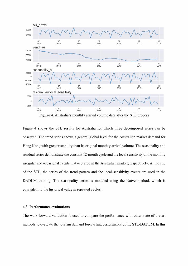
Figure 4. Australia’s monthly arrival volume data after the STL process

Figure 4 shows the STL results for Australia for which three decomposed series can be

observed. The trend series shows a general global level for the Australian market demand for

Hong Kong with greater stability than its original monthly arrival volume. The seasonality and

residual series demonstrate the constant 12-month cycle and the local sensitivity of the monthly

irregular and occasional events that occurred in the Australian market, respectively. At the end

of the STL, the series of the trend pattern and the local sensitivity events are used in the

DADLM training. The seasonality series is modeled using the Naïve method, which is

equivalent to the historical value in repeated cycles.

4.3. Performance evaluations

The walk-forward validation is used to compare the performance with other state-of-the-art

methods to evaluate the tourism demand forecasting performance of the STL-DADLM. In this

subsection, the validation setting for the experiments is introduced and the forecasting results

on one- and multiple-step forecasting are compared.

4.3.1. Validation setup

The walk-forward validation method is used to simulate the real-world forecasting scenario;

the new tourism arrival volume data are available at the end of the month and used for the

following month (Law et al., 2019). In the forecasting process, the time step window is initially

set to 24 months (2012–2013) for the training data, which is then augmented for each time step

by a month to forecast the next month/s.

Following this validation setup, SVR, extreme gradient boosting tree regressor

(XGBTR), ANN model (Palmer, Montano & Sesé, 2006), ARIMA, DLM (Law et al., 2019),

ETS, and Naïve methods are used as baseline models. We investigate the robustness of the

proposed STL-DADLM compared with all these baseline models in the experiment. The STL-

DADLM uses the global trend pattern and local sensitivity series in the experiment, whereas

baseline models utilize the original tourism arrival volume. Based on the previous n-month

data <{𝑥$}$'3*%3 , {𝑦$}$'3*%3 B and to predict the next month, the inputs for ANN, DLM, and

DADLM are the same and thus forms a 3D array. The first dimension is the total number of

months in training, followed by the time-step dimension of n, and then the factor vector created

by the SII data and tourism arrival volumes of the corresponding months. Moreover, SVR and

XGBTR utilize the past n-month data <{𝑥$}$'3*%3 , {𝑦$}$'3*%3 B to predict the tourism arrival

volume for the next month{𝑦$}$'3(".

The time step n is evaluated from the grid search for ANN, DLM, DADLM, SVR, and

XGBTR. However, different from the inputs of ANN, DLM, and DADLM, those for SVR and

XGBTR are transformed into 2D array by flattening the original 3D array. The result is a large-

size input in the second dimension due to the flattened array in these models. Therefore, SVR

and XGBTR adopts the maximal information coefficient MIC (e.g. Kinney & Atwal, 2014) to

conduct feature engineering in forecasting. The ANN model has three layers, including an

initial hidden layer size of 64. Law et al. (2019) established a default setting for the DLM

model and initialized a size of 256 on the LSTM hidden layer and 32 on the dense layers before

the output layer. The ARIMA model uses the tourism arrival volume as input and

autoregressive parameter; the non-seasonal differences and moving average terms are validated

in the subsequent stage.

Next, grid search is implemented for parameter tuning through walk-forward validation

to determine the best performance among all compared algorithms. To reduce the search

complexity, the number of hidden layers and dropout rates in the DL and ANN are set with a

limited option based on common DL model specifics (Goodfellow, Bendigo & Courville,

2016). For ANN, the hidden layer is selected through grid search from the range {64,128,256}

on each tourism source market data. For DLM, the hidden and dense layers of LSTM are

respectively selected through grid search from the ranges {128,256,512} and {32,64,128} on

each tourism source market data. Prior to the forecasting experiment, several parameters must

be tuned particularly for DADLM, such as the size of the hidden unit in LSTM ∈

{128,256,512} , the dropout rate 𝑑 ∈ {0.01,0.3,0.5} , and the size of the dense layer 𝑞 ∈

{32,64,128},. By contrast, the autoregressive parameter, non-seasonal differences, and the

moving average parameter for ARIMA are determined first through the Box–Jenkins

methodology for obtaining several candidate models (Zhang, 2013). Then the grid search is

used with Akaike’s information criterion to identify the best ARIMA model with parameters.

The time step for the training data are also identified from range of 𝑛 ∈ {12,13,14,15}. Given

the limited data length of 72 months, the time step length for the training data capped at 15 and

12 months is the most satisfactory. As a result, all parameters are determined using the grid

search on the walk-forward validation, and the final parameter is the set with the lowest training

loss.

The root mean square error (RMSE), mean absolute error (MAE), and MAPE are used

to measure the forecasting performance and compare their effectiveness, as below.

𝑅𝑀𝑆𝐸 = ]"1∑ 1,'" ^𝑦$, − 𝑦$,

^`#

(14),

𝑀𝐴𝐸 = "1∑ 1,'" a𝑦$, − 𝑦$,

^a (15),

𝑀𝐴𝑃𝐸 = "1∑ 1,'" S4#

!*4#!^

4#!S × 100% (16).

4.3.2. Evaluation of one-step forecasting

In one-step forecasting, the tourism arrival volume data are collected from July 2012 to June

2014 and used as training to forecast the monthly predictions for the six visitor markets. The

STL-DADLM processes the data from July 2014 to June 2018 (48 months) using a step-by-

performance step approach with a walk-forward validation on each visitor market to determine

its robustness compared with that of the baseline models. DLDAM without STL decomposition

is also included in the comparison to verify the effect of STL decomposition in the time series

forecasting.

After the forecasting process, we obtain the overall results of the 48 months data for

each visitor market. The averages of the error rate on each evaluation metrics (MAPE, RMSE,

and MAE) are computed using the predicted and actual tourism arrival volumes for each visitor

market. Tables 2, 3, and 4 summarize the comparison of the forecasting results for the tourism

arrival volume using the proposed method and the baseline models.

Table 2: Short-term forecasting MAPE comparison for four years in six source markets

METHOD MAPE

AU GB PH TH SG US STL-DADLM 1.09 1.30 1.63 1.94 1.15 1.11

DADLM* 1.78 2.13 2.10 2.19 1.63 1.45 DLM 1.93 2.20 2.65 2.79 2.20 1.93 ANN 7.01 7.90 8.60 17.12 16.76 5.33

ARIMA 8.11 7.51 6.12 12.91 15.11 4.29 XGBTR 10.68 7.59 13.09 13.61 19.75 7.09

SVR 11.84 9.28 8.48 12.32 12.99 7.26 ETS 8.89 9.10 10.16 14.23 13.78 8.33

NAIVE 10.39 8.15 11.38 15.76 19.92 6.78 * without the STL method Table 3: Short-term forecasting RMSE comparison for four years in the six source markets

METHOD RMSE

AU GB PH TH SG US STL-DADLM 769.02 770.49 1465.87 1399.55 1107.91 1262.07

DADLM* 1160.46 1299.96 2023.13 1612.86 1642.27 1734.13 DLM 1262.63 1348.43 2407.91 2094.97 1868.86 2327.32 ANN 4154.11 4366.58 7062.08 8510.22 9582.21 6448.46

ARIMA 4615.20 4522.91 6079.81 7911.52 9231.17 5167.16 XGBTR 5826.28 4588.56 11017.62 8171.16 10283.26 8606.05

SVR 6267.49 6269.72 7404.01 7807.10 8548.92 8918.57 ETS 4817.92 6109.22 8097.37 8322.90 8790.93 9318.77

NAIVE 5802.13 4418.89 8613.23 8402.56 10291.19 8568.32 * without the STL method

Table 4: Short-term forecasting MAE comparison for four years in the six source markets

METHOD MAE AU GB PH TH SG US

STL-DADLM 559.49 574.20 1129.37 910.69 652.84 1005.51 DADLM* 868.24 933.45 1524.38 1193.60 952.76 1376.83

DLM 929.05 985.65 1868.19 1325.67 1101.59 1766.68 ANN 3385.25 3712.68 5728.29 7004.80 7069.82 5224.06

ARIMA 3655.21 3577.27 4779.32 6135.98 6988.13 4236.29 XGBTR 4442.41 3645.38 8913.38 6294.59 8347.91 7044.53

SVR 4754.78 4698.96 5657.40 6074.85 6754.51 7066.07 ETS 3776.89 4519.90 7716.13 6416.29 6813.62 7312.56

NAIVE 4412.67 3789.17 8132.33 6722.81 8521.83 6927.02 * without the STL method

Among all compared methods, the STL-DADLM achieved the best forecasting performance

in terms of the minimum error rate on all evaluation metrics across all six source markets. The

STL-DADLM forecasting error rate is lower than those of ANN, ARIMA, SVR, XGBTR,

Naïve and ETS. The mean forecasting MAPE of Australia after applying STL on the DADLM

decreased from 1.78% to 0.78%, compared with that of the DADLM without STL. This result

suggests that in the case of Hong Kong tourism demand, STL can further enhance the

forecasting accuracy without requiring additional data.

Interestingly, the forecasting error rates of the STL-DADLM and DADLM without STL

decomposition are lower than those of DLM for the six source markets. These results confirm

that DADLM with the duo attention layer has a clear advantage in multivariate time series

forecasting in terms of the efficient selection of explanatory variables (i.e., SII factors).

Moreover, STL-DADLM outperforms DADLM and DLM in forecasting accuracy.

Table 5: Diebold-Mariano test results of short-term forecasting MAPE for four years in six

visitor markets

METHOD MARKETS DIEBOLD-MARIANO STATISTICS

DADLM* DLM ANN ARIMA XGBTR SVR ETS NAIVE

STL-DADLM

AU 2.211 5.189 2.135 5.122 3.191 −5.163 5.893 2.731 GB 3.901 2.178 −3.136 3.188 −3.122 −4.132 5.787 2.872 PH 2.876 −2.788 −2.873 3.982 −2.312 −2.331 2.121 2.092 TH 3.192 −5.213 5.782 3.823 −2.992 −3.120 2.110 2.019 SG 2.918 2.123 2.111 4.132 2.782 −4.882 3.782 3.892 US −2.903 −3.723 3.652 −3.121 2.731 5.172 3.772 5.172

* The DADLM experiment does not use the STL decomposition method.

Table 5 suggests that the STL-DADLM is significantly better than other models in reducing

the MAPE according to Diebold–Mariano test at 0.05 statistical significance. The null

hypothesis of the STL-DADLM (non-rejection of MAPE) obtains the same forecasting

accuracy as the other models.

4.3.3. Evaluation of multiple-step forecasting

In this experiment, STL-DADLM uses the data from the previous 12 months

<{𝑥$}$'3*""3 , {𝑦$}$'3*""3 B to forecast the next three and six months data during the multiple-

step forecasting. Other baseline models, such as SVR and XGBTR, need to process numerous

steps because they use ETS to forecast the SII factors for the next three and six months; the SII

data are not available prior to the end of the new month. However, the LSTM-based STL-

DADLM, DLM, and ANN naturally output multiple dimensional vector using the previous 12-

month data. The one-step forecasting presented in the previous section and the multiple-step

forecasting in this subsection are based on the walk-forward validation. The difference is that

the former only forecasts one month per time step, whereas the latter forecasts multiple months

per time step.

Table 6: Long-term forecasting MAPE comparison for four years in the six source markets

METHOD MAPE

AU GB PH TH SG US

STL-DADLM-3 MONTHS 4.48 4.54 5.04 6.21 6.33 4.12

DLM-3 MONTHS 5.60 5.31 6.97 7.41 6.37 4.55

ANN-3 MONTHS 6.19 5.92 7.89 9.18 7.33 5.16

ARIMA-3 MONTHS 8.99 7.28 9.13 10.33 8.09 6.18

XGBTR-3 MONTHS 7.12 7.79 8.33 11.23 9.17 10.13

SVR-3 MONTHS 8.22 7.83 8.93 9.13 7.56 10.18

ETS-3 MONTHS 9.20 9.11 10.31 12.11 10.09 11.33

NAÏVE-3 MONTHS 10.22 10.02 11.23 13.01 13.10 12.08

STL-DADLM-6 MONTHS 4.57 4.05 4.65 8.97 8.03 4.50

DLM-6 MONTHS 5.74 5.72 5.47 8.91 8.47 6.33

ANN-6 MONTHS 5.89 6.33 7.17 9.23 9.02 7.82

ARIMA-6 MONTHS 9.12 9.33 8.19 10.32 10.11 11.14

XGBTR-6 MONTHS 11.12 12.32 9.76 9.39 10.35 12.63

SVR-6 MONTHS 10.25 11.18 9.98 9.95 11.76 11.83

ETS-6 MONTHS 12.30 13.21 11.35 11.09 12.78 13.88

NAÏVE-6 MONTHS 12.92 13.56 12.60 12.93 13.02 13.90

* The MAPE error in the table is the average MAPE across the forecasting period.

Table 7: Long-term forecasting RMSE comparison for four years in the six source markets

METHOD RMSE

AU GB PH TH SG US

STL-DADLM-3 MONTHS 2634.46 2723.67 5083.31 4185.16 4613.50 5035.57

DLM-3 MONTHS 3119.11 3090.29 6493.31 4215.15 4660.23 5725.94

ANN-3 MONTHS 3810.32 3817.21 7013.35 7919.28 5910.23 6322.65

ARIMA-3 MONTHS 5983.13 4339.11 9132.98 8720.19 6793.07 7013.78

XGBTR-3 MONTHS 4514.19 5117.29 8239.09 9018.19 8190.32 10391.98

SVR-3 MONTHS 5218.33 5313.11 8819.21 7831.33 5953.67 11882.12

ETS-3 MONTHS 6310.33 5919.20 9763.03 10031.31 9201.73 12893.72

NAÏVE-3 MONTHS 6900.29 6509.12 11903.22 11290.62 12192.63 13356.15

STL-DADLM-6 MONTHS 2830.17 2198.69 4756.12 5145.76 5212.93 5422.20

DLM-6 MONTHS 3712.37 3328.58 5315.06 5098.62 5298.56 7818.35

ANN-6 MONTHS 3819.21 3928.73 6713,12 5728.82 6019.22 8718.09

ARIMA-6 MONTHS 8193.03 8930.01 7109.11 7991.01 6837.31 11020.03

XGBTR-6 MONTHS 9010.78 11211.13 8982.16 6387.27 6928.13 12872.28

SVR-6 MONTHS 8639.72 10113.23 9317.73 6827.19 7139.29 11398.83

ETS-6 MONTHS 10201.98 12390.82 10982.76 8618.17 7539.27 13562.18

NAÏVE-6 MONTHS 10332.63 13101.87 12301.10 9031.09 7763.12 13671.02

* The RMSE error in the table is the average RMSE across the forecasting period.

Table 8: Long-term forecasting MAE comparison for four years in the six source markets

METHOD MAE

AU GB PH TH SG US

STL-DADLM-3 MONTHS 2029.46 2157.55 3697.42 3682.75 2926.41 4213.21

DLM-3 MONTHS 2481.58 2589.91 4966.95 3795.97 2945.77 4571.10

ANN-3 MONTHS 3512.12 2918.87 5890.02 6782.92 4010.03 5287.67

ARIMA-3 MONTHS 4519.21 3982.09 7390.23 7201.03 4590.21 6013.32

XGBTR-3 MONTHS 3819.01 4013.22 6367.56 7516.29 5010.11 8039.07

SVR-3 MONTHS 4211.52 4136.50 6989.20 6720.83 4209.91 8047.29

ETS-3 MONTHS 4710.33 4311.09 7537.12 8036.92 5493.40 8911.19

NAÏVE-3 MONTHS 5012.02 4539.10 8011.83 8536.10 6219.90 9782.12

STL-DADLM-6 MONTHS 2236.43 1923.37 3436.25 4142.05 3711.07 4663.74

DLM-6 MONTHS 2869.88 2798.37 3943.27 4087.29 4053.55 6748.24

ANN-6 MONTHS 3011.18 4012.02 4527.73 4590.09 4928.11 7818.30

ARIMA-6 MONTHS 5809.90 7019.82 5390.02 5310.07 5822.03 9011.38

XGBTR-6 MONTHS 6321.98 9011.17 6098.28 4662.27 5919.90 9892.53

SVR-6 MONTHS 6109.92 8673.25 6209.81 5019.53 6298.73 9109.80

ETS-6 MONTHS 6610.30 9593.01 7102.90 5722.77 6536.29 13102.92

NAÏVE-6 MONTHS 6732.11 9710.22 7430.88 6103.24 6630.21 13221.17

* The MAE error in table is the average MAE across the forecasting period

Tables 6, 7, and 8 present the error rates in the three- and six-month step forecasting

performances of all baseline models for all six source markets. The error rates of STL-DADLM

and DLM are significantly smaller than those of the other models. For the three- and six-month

step forecasting, the same period (July 2014 to June 2018) is used as the testing data for all six

source market arrival data to validate the forecasting performance. The average error rates

(MAPE, RMSE, and MAE) over the period of July 2014 to June 2018 are used to evaluate the

model performances.

The average error rate of MAPE for the three-month step forecasting by STL-DADLM

is significantly lower than that of the other models (Table 6) (Law et al., 2019). The STL

improved the forecast accuracy without requiring additional data and the duo attention layer

utilized the SII factors to reduce the overfitting. The same results can be observed in the three-

month step forecasting in Tables 7 and 8.

For the average error rate on the six-month step forecasting, the proposed framework

obtains a remarkably lower value than that of DADLM, DLM, ARIMA, ANN, XGBTR, and

SVR for all source markets except Thailand. The average error rates of STL-DADLM,

DADLM, and DLM for the visitor market of Thailand are equal. This finding may be explained

by the generalized SII data for all visitor markets of Hong Kong tourism demand, some of

which may be ineffective due to language and cultural differences across different visitor

markets. However, for the other five source markets, the STL-DADLM achieved a significantly

lower average error rate than the other baseline models. For Great Britain, the average MAPE

is reduced from 5.72% to 4.05% compared with that of STL-DADLM and DLM. Similar

results are observed in Tables 7 and 8.

Table 9: Diebold-Mariano Test results of long-term forecasting MAPE for four years in six

visitor markets

METHOD DIEBOLD-MARIANO STATISTICS

DLM-3 months

ANN-3 months

ARIMA-3 months

XGBTR-3 months

SVR-3 months

ETS-3 months

Naïve-3 months

AU 2.13 2.39 −4.01 5.20 5.78 3.33 5.11

GB −3.10 2.89 2.01 3.09 −4.22 3.89 5.09

PH 5.14 −5.09 2.00 3.11 -3.14 7.09 10.38

TH 3.11 −4.02 2.09 2.40 -2.83 9.19 9.17

SG 2.90 −3.13 3.17 2.28 −2.98 8.17 9.11

US −5.10 −2.30 -2.71 2.21 −5.31 5.87 6.02

METHOD DIEBOLD-MARIANO STATISTICS

DLM-6 months

ANN-6 months

ARIMA-6 months

XGBTR-6 months

SVR-6 months

ETS-6 months

Naïve-6 months

AU 3.10 −3.19 2.90 −3.18 2.02 −8.10 −7.66

GB 2.99 −3.38 2.13 −2.31 2.88 −8.17 −7.91

PH 3.82 −3.92 2.67 −3.34 2.91 −9.10 −4.16

TH −3.11 −4.12 3.18 −3.09 5.13 −10.17 −6.82

SG 2.90 −5.60 3.80 2.89 5.19 −5.22 −5.19

US 2.09 2.92 2.67 2.80 5.89 −6.83 −9.12

Table 9 shows the results of the Diebold–Mariano test for 2014 to 2018 in the six source

markets for long-term forecasting. In most of the source markets, STL-DADLM outperforms

the other models at 0.05 significance level. The results show that for most cases, the mean

MAPE of STL-DADLM is lower than that of the benchmark models on three- and six-month

step forecasting.

In summary, the STL of the tourism arrival volume data series can be accurately

predicted in short- and long-term forecasting without further requirements. STL can further

reduce the forecast overfitting by avoiding the complex models on the basis of the available

data. Compared with DLM, the duo attention layer from DADLM efficiently uses the

forecasting features with higher accuracy. The DL methods with attention mechanism (i.e.,

DLM and DADLM) achieve substantial improvements on forecasting compared with the

traditional models. Moreover, the STL-DADLM reduces the overfitting problem in tourism

demand forecasting and generates lower average error rate compared with the baseline models

for short- and long-term forecasting.

5. CONCLUSIONS

This research proposes a new framework, STL-DADLM, to reduce overfitting and improve the

tourism demand forecasting. First, using the data from a case study involving six source

markets for Hong Kong, we decomposed the tourism arrival volume using STL, which

increased the forecasting accuracy. Second, the efficiency of the feature and lag order selection

are improved using the duo attention layer to reduce the model overfitting. The proposed DL

forecasting model achieved higher accuracy than the existing models.

The new forecasting framework presents important implications for tourism practice.

Tourism practitioners can benefit from the improved accuracy of the novel DL forecasting

models. Specifically, effective short-term planning and decision-making and reliable long-term

strategies and risk management can be implemented. After comparing several tourism

forecasting methods, we alleviate the overfitting issue using data decomposition and the duo

attention layer in DADLM to increase the accuracy of tourism demand forecast. The model

robustness is evaluated by comparison with commonly used models, such as DLM, ANN,

ARIMA, SVR, XGBTR, ETS, and Naïve methods. This study offers two important

contributions to tourism literature.

First, we use the STL decompositions to address the overfitting problem caused by the

limited data volume in DL networks. The limited data are decomposed into stationary subseries

and the forecasting performance improved without further requirements on one- and multiple-

step forecasting. Second, we develop the DADLM model by adding an extra attention

mechanism into DLM. The empirical results confirm that the duo attention layer can efficiently

conduct the feature and lag order selection, which is a remarkable improvement. In addition,

the explanatory variables (SII factors) are also efficiently utilized and identified with high

accuracy. In conclusion, the duo attention layer can alleviate the overfitting issue in Hong Kong

tourism demand forecasting.

This research, however, has several limitations. Considering that DL requires a large

number of parameters for optimization, future research should concentrate on investigating the

forecasting stability. To facilitate such research, we release our dataset “HK2012–2018” at

https://github.com/tulip-lab/open-data and the implementation “STL-DADLM” as open source

at https://github.com/tulip-lab/open-code. Furthermore, using the available data sources,

superior determinants such as the economy, climate change, and leisure time, can also be used

as potential explanatory variables. Given the present health crisis caused by the spread of the

corona virus, and the challenges faced by the global tourism face, any tourism destination can

encounter various natural, economic, political and safety crises that can lead to an external

shock and unforeseen decline in demand. The resilience and adaptiveness of a tourism

destination, however, is highly influenced by how governments and tourism actors respond to

crisis (Hystad and Keller, 2008). Moreover, tourism can assist in the recoveries of the

destinations (Muskat, Nakanishi & Blackman, 2014).

REFERENCES

Assaf, A. G., Li, G., Song, H., & Tsionas, M. G. (2019). Modeling and forecasting regional tourism demand using the Bayesian global vector autoregressive (BGVAR) model. Journal of Travel Research, 58(3), 383-397.

Bangwayo-Skeete, P. F., & Skeete, R. W. (2015). Can Google data improve the forecasting performance of tourist arrivals? Mixed-data sampling approach. Tourism Management, 46, 454-464.

Baldigara T., & Mamula M. (2015). Modelling International Tourism Demand Using Seasonal ARIMA Models Tourism and Hospitality Management, 21(1), 19-31.

BoardKong TourismHong. (2017). A Statistical Review of Hong Kong Tourism, 2017. http://partnernet.hktb.com, accessed on 02.11.2019.

Cai, Z. J., Lu, S., & Zhang, X. B. (2009). Tourism demand forecasting by support vector regression and genetic algorithm. In 2009 2nd IEEE International Conference on Computer Science and Information Technology, Beijing, (pp. 144-146).

Camacho, M., & Pacce, M. J. (2018). Forecasting travellers in Spain with Google’s search volume indices. Tourism Economics, 24(4), 434-448.

Cankurt, S. (2016). Tourism demand forecasting using ensembles of regression trees. In 2016 IEEE 8th International Conference on Intelligent Systems (IS), Madeira Island, Portugal, (pp. 702-708).

Chamberlin G. (2010). Googling the present. Economic & Labour Market Review, 4, 59-95. Chen, J. L., Li, G., Wu, D. C., & Shen, S. (2019). Forecasting seasonal tourism demand using

a multi-series structural time series method. Journal of Travel Research, 58(1), 92-103. Chen, H. K., & Wu, C. J. (2012). Travel time prediction using empirical mode decomposition

and gray theory: Example of National Central University bus in Taiwan. Transportation Research Record, 2324(1), 11-19.

Che, Z., Purushotham, S., Cho, K., Sontag, D., & Liu, Y. (2018). Recurrent neural networks for multivariate time series with missing values. Scientific Reports, 8(1), 6085.

Choi, H. & Varian Hal. (2012). Predicting the Present with Google Trends. The Economic Record, 88, 2-9.

Cleveland, B.R., Cleveland, S.W., McRae E.J., & Terpenning, I. (1990). STL: A Seasonal-Trend Decomposition. Journal of Official Statistics, 6, 3-73.

Claveria, O., Monte, E., & Torra, S. (2015). Tourism demand forecasting with neural network models: different ways of treating information. International Journal of Tourism Research, 17(5), 492-500.

Connor, J.T., Martin, R.D., & Atlas, L.E. (1994). Recurrent neural networks and robust time series prediction. IEEE Transactions on Neural Networks, 5(2), 240-54.

Coshall, J. (2000). Spectral analysis of international tourism flows. Annals of Tourism Research, 27, 577-589.

Fesenmaier, D. R., Xiang, Z., Pan, B., & Law, R. (2011). A framework of search engine use for travel planning. Journal of Travel Research, 50(6), 587-601.

Frechtling, D. (2012). Forecasting tourism demand. Abingdon, UK: Routledge. Gers, F.A., Eck, D., & Schmidhuber, J. (2000). Applying LSTM to Time Series Predictable

through Time-Window Approaches. ICANN. Giles, C. L., Lawrence, S., & Tsoi, A. C. (2001). Noisy time series prediction using recurrent neural networks and grammatical inference. Machine Learning, 44(1-2), 161-183.

Goh, C., & Law, R. (2002). Modeling and forecasting tourism demand for arrivals with stochastic nonstationary seasonality and intervention. Tourism Management, 23(5), 499-510.

Goodfellow, I., Bengio, Y., & Courville, A. (2016). Deep Learning. Cambridge, MA: MIT Press.

Gunter, U., & Önder, I. (2016). Forecasting city arrivals with Google Analytics. Annals of Tourism Research, 61, 199-212.

Hassani, H., Silva, E. S., Antonakakis, N., Filis, G., & Gupta, R. (2017). Forecasting accuracy evaluation of tourist arrivals. Annals of Tourism Research, 63, 112-127.

Hawkins, D. M. (2004). The problem of overfitting. Journal of chemical information and computer sciences, 44(1), 1-12.

Huang, N. E., Shen, Z., Long, S. R., Wu, M. C., Shih, H. H., Zheng, Q., ... & Liu, H. H. (1998). The empirical mode decomposition and the Hilbert spectrum for nonlinear and non-stationary time series analysis. Proceedings of the Royal Society of London. Series A: Mathematical, Physical and Engineering Sciences, 454(1971), 903-995.

Hystad P., W., Keller P.C. (2008). Towards a destination tourism disaster management framework: long-term lessons from a forest fire disaster. Tourism Management, 1, 151-162.

Khashei, M., & Bijari, M. (2011). A novel hybridization of artificial neural networks and ARIMA models for time series forecasting. Applied Soft Computing, 11(2), 2664-2675.

Kinney, J. B., & Atwal, G. S. (2014). Equitability, mutual information, and the maximal information coefficient. Proceedings of the National Academy of Sciences, 111(9), 3354-3359.

Law, R., Li, G., Fong, D. K. C., & Han, X. (2019). Tourism demand forecasting: A deep learning approach. Annals of Tourism Research, 75, 410-423.

LeCun, Y., Bengio, Y., & Hinton, G. (2015). Deep learning. Nature, 521(7553), 436-444. Lim, C., McAleer, M., & Min, J. C. (2009). ARMAX modelling of international tourism

demand. Mathematics and Computers in Simulation, 79(9), 2879-2888. Li, G., Song, H., & Witt, S. (2005). Recent Development in Econometric Modelling and

Forecasting. Journal of Travel Research, 44(1), 82-99. Liu, H., Lu, J., Feng, J., & Zhou, J. (2017). Group-aware deep feature learning for facial age

estimation. Pattern Recognition, 66, 82-94. Li, X., Pan, B., Law, R., & Huang, X. (2017). Forecasting tourism demand with composite

search index. Tourism Management, 59, 57-66. Li, X., & Law, R. (2020). Forecasting tourism demand with decomposed search cycles. Journal

of Travel Research, 59(1), 52-68. Long, W., Liu, C., & Song, H. (2019). Pooling in tourism demand forecasting. Journal of

Travel Research, 58(7), 1161-1174. Ma, Y., Xiang, Z., Du, Q., & Fan, W. (2018). Effects of user-provided photos on hotel review

helpfulness: An analytical approach with deep learning. International Journal of Hospitality Management, 71, 120-131.

Muskat, B., Nakanishi, H., & Blackman, D. (2014). Integrating Tourism into Disaster Recovery Management: The Case of the Great East Japan Earthquake and Tsunami 2011. In B. Ritchie, & K. Campiranon (Eds.), Tourism Crisis and Disaster Management in Asia-Pacific (pp. 97–115). Wallingford, UK.

Niu, W., Li, G., Zhao, Z., Tang, H., & Shi, Z. (2011). Multi-granularity context model for dynamic Web service composition. Journal of network and computer applications, 34(1), 312-326.

Önder, I. (2017). Forecasting tourism demand with Google trends: Accuracy comparison of countries versus cities. International Journal of Tourism Research, 19(6), 648-660.

Ognjanov, B., Tang, Y., & Turner, L. (2018). Forecasting International Tourism Regional Expenditure. Chinese Business Review, 17(1), 38-52.

Palmer, A., Montano, J. J., & Sesé, A. (2006). Designing an artificial neural network for forecasting tourism time series. Tourism Management, 27(5), 781-790.

Park, S., Lee, J., & Song, W. (2017). Short-term forecasting of Japanese tourist inflow to South Korea using Google trends data. Journal of Travel & Tourism Marketing, 34(3), 357-368.

Peng, B., Song, H., & Crouch, G. I. (2014). A meta-analysis of international tourism demand forecasting and implications for practice. Tourism Management, 45, 181-193.

Qiu, H., Fan, D. X., Lyu, J., Lin, P. M., & Jenkins, C. L. (2019). Analyzing the Economic Sustainability of Tourism Development: Evidence from Hong Kong. Journal of Hospitality & Tourism Research, 43(2), 226-248.

Qiu, X., Ren, Y., Suganthan, P. N., & Amaratunga, G. A. (2017). Empirical mode decomposition-based ensemble deep learning for load demand time series forecasting. Applied Soft Computing, 54, 246-255.

Saayman, A., Viljoen, A., & Saayman, M. (2018). Africa’s outbound tourism: An Almost Ideal Demand System perspective. Annals of Tourism Research, 73, 141-158.

Scharkow, M., & Vogelgesang, J. (2011). Measuring the public agenda using search engine queries. International Journal of Public Opinion Research, 23(1), 104-113.

Shen, S., Li, G., & Song, H. (2011). Combination forecasts of international tourism demand. Annals of Tourism Research, 38(1), 72-89.

Silva, E. S., Hassani, H., Heravi, S., & Huang, X. (2019). Forecasting tourism demand with denoised neural networks. Annals of Tourism Research, 74, 134-154.

Smeral, E. (2019). Seasonal forecasting performance considering varying income elasticities in tourism demand. Tourism Economics, 25(3), 355-374.

Song, H., & Li, G. (2008). Tourism demand modelling and forecasting—A review of recent research. Tourism Management, 29(2), 203-220.

Song, H., Dwyer, L., Li, G., & Cao, Z. (2012). Tourism economics research: A review and assessment. Annals of Tourism Research, 39(3), 1653-1682.

Sun, S., Wei, Y., Tsui, K. L., & Wang, S. (2019). Forecasting tourist arrivals with machine learning and internet search index. Tourism Management, 70, 1-10.

Theodosiou, M. (2011). Forecasting monthly and quarterly time series using STL decomposition. International Journal of Forecasting, 27(4), 1178-1195.

Wan, S.K., & Song, H. (2018). Forecasting turning points in tourism growth. Annals of Tourism Research, 72, 156-167.

Wang, X., Li, G., Jiang, G., & Shi, Z. (2013). Semantic trajectory-based event detection and event pattern mining. Knowledge and information systems, 37(2), 305-329.

Wu, Z., & Huang, N. E. (2009). Ensemble empirical mode decomposition: a noise-assisted data analysis method. Advances in Adaptive Data Analysis, 1(1), 1-41.

Wong, K. K., Song, H., & Chon, K. S. (2006). Bayesian models for tourism demand forecasting. Tourism Management, 27(5), 773-780.

Yu, J. X., Ng, M. K., & Huang, J. Z. (2001). Patterns discovery based on time-series decomposition. In Pacific-Asia Conference on Knowledge Discovery and Data Mining, Hong Kong, (pp. 336-347).

Yahya, N. A., Samsudin, R., & Shabri, A. (2017). Tourism forecasting using hybrid modified empirical mode decomposition and neural network. International Journal of Advances in Soft Computing and its Applications, 9, 14-31.

Yang, Y., Pan, B., & Song, H. (2014). Predicting hotel demand using destination marketing organization’s web traffic data. Journal of Travel Research, 53(4), 433-447.

Yang, Y., & Zhang, H. (2019). Spatial-temporal forecasting of tourism demand. Annals of Tourism Research, 75, 106-119.

Zhang, G. P. (2003). Time series forecasting using a hybrid ARIMA and neural network model. Neurocomputing, 50, 159-175.

Zhang, Y., Li, G., Muskat, B., Law, R., & Yang, Y. (2020). Group pooling for deep tourism demand forecasting. Annals of Tourism Research, 82, 102899.

Zhang, X., & Wang, J. (2018). A novel decomposition‐ensemble model for forecasting short‐term load‐time series with multiple seasonal patterns. Applied Soft Computing, 65, 478-494.

Zheng, A., & Casari, A. (2018). Feature engineering for machine learning: Principles and techniques for data scientists (1st ed.). Sebastopol, CA: O'Reilly.