topsis for solving multi-attribute decision making...

New Trends in Neutrosophic Theory and Applications

65

PARTHA PRATIM DEY1, SURAPATI PRAMANIK2, *, BIBHAS C. GIRI3

1, 3 Department of Mathematics, Jadavpur University, Kolkata-700032, West Bengal, India. 2* Department of Mathematics, Nandalal Ghosh B.T. College, Panpur, P.O.-Narayanpur, District North 24 Parganas, Pin code-743126, West Bengal, India. Corresponding author’s E-mail: [email protected]

TOPSIS for Solving Multi-Attribute Decision Making Problems

under Bi-Polar Neutrosophic Environment

Abstract The paper investigates a technique for order preference by similarity to ideal solution (TOPSIS)

method to solve multi-attribute decision making problems with bipolar neutrosophic information. We define Hamming distance function and Euclidean distance function to determine the distance between bipolar neutrosophic numbers. In the decision making situation, the rating of performance values of the alternatives with respect to the attributes are provided by the decision maker in terms of bipolar neutrosophic numbers. The weights of the attributes are determined using maximizing deviation method. We define bipolar neutrosophic relative positive ideal solution (BNRPIS) and bipolar neutrosophic relative negative ideal solution (BNRNIS). Then, the ranking order of the alternatives is obtained by TOPSIS method and most desirable alternative is selected. Finally, a numerical example for car selection is solved to demonstrate the applicability and effectiveness of the proposed approach and comparison with other existing method is also provided.

Keywords

Single valued neutrosophic sets; bipolar neutrosophic sets; TOPSIS; multi-attribute decision making.

1. Introduction Zadeh [1] introduced the concept of fuzzy set to deal with problems with imprecise information

in 1965. However, Zadeh [1] considers one single value to express the grade of membership of the fuzzy set defined in a universe. But, it is not always possible to represent the grade of membership value by a single point. In order to overcome the difficulty, Turksen [2] incorporated interval valued fuzzy sets. In 1986, Atanassov [3] extended the concept of fuzzy sets [1] and defined intuitionistic fuzzy sets which are characterized by grade of membership and non-membership functions. Later, Lee [4, 5] introduced the notion of bipolar fuzzy sets by extending the concept of fuzzy sets where the degree of membership is expanded from [0, 1] to [-1, 1]. In a bipolar fuzzy set, if the degree of membership is zero then we say the element is unrelated to the corresponding property, the membership degree (0, 1] of an element specifies that the element somewhat satisfies

mailto:[email protected]

Florentin Smarandache, Surapati Pramanik (Editors)

66

the property, and the membership degree [−1, 0) of an element implies that the element somewhat satisfies the implicit counter-property [6]. Zhou and Li [7] incorporated the notion of bipolar fuzzy semirings and investigated relative properties using positive t- cut, negative s- cut and equivalence relation. Smarandache [8, 9, 10, 11] incorporated indeterminacy membership function as independent component and defined neutrosophic set on three components truth, indeterminacy and falsehood. However, from practical point of view, Wang et al. [12] defined single valued neutrosophic sets (SVNSs) where degree of truth membership, indeterminacy membership and falsity membership [0, 1]. Deli et al. [13] introduced the notion of bipolar neutrosophic sets (BNSs) which is a generalization of the fuzzy sets, bipolar fuzzy sets, intuitionistic fuzzy sets, neutrosophic sets. Pramanik and Mondal defined rough bipolar neutrosophic set [14].

Zhang and Wu [15] presented a TOPSIS [16] method for solving single valued neutrosophic multi-criteria decision making with incomplete weight information. Chi and Liu [17] proposed an extended TOPSIS method for MADM problems where the attribute weights are unknown and the attribute values are expressed in terms of interval neutrosophic numbers. Biswas et al. [18] developed a new TOPSIS based approach for solving multi-attribute group decision making problem with simplified neutrosophic information. Broumi et al. [19] extended TOPSIS method for multiple attribute decision making based on interval neutrosophic uncertain linguistic variables. In neutrosophic hybrid environment, Pramanik et al. [20] extended TOPSIS method for singled valued soft expert set based multi-attribute decision making problems. Dey et al. [21] presented TOPSIS method for generalized neutrosophic soft multi-attribute group decision making. Mondal et al. [22] presented TOPSIS in rough neutrosophic environment and provided illustrative example.

Deli et al. [13] investigated a bipolar neutrosophic multi-criteria decision making approach based on bipolar neutrosophic weighted average and geometric operators and the score, certainty and accuracy functions. Uluçay et al. [23] studied similarity measures of bipolar neutrosophic sets and their application to multiple criteria decision making. Literature review suggests that TOPSIS method in bipolar neutrosophic environment is yet to appear. Therefore this issue needs to be addressed.

In this paper, we define Hamming distances and Euclidean distances between two BNSs and develop a new TOPSIS based method for solving MADM problems under bipolar neutrosophic assessments.

The content of the paper is organized as follows. Section 2 presents some basic definitions concerning neutrosophic sets, SVNSs, BNSs which are helpful for the construction of the paper. Hamming and Euclidean distances between two bipolar neutrosophic numbers (BNNs) are also defined in the Section 2. Section 3 is devoted to present TOPSIS method for MADM problems under bipolar neutrosophic environment. A car selection problem is solved in Section 4 to illustrate the applicability of the proposed method. Sectin 5 presents conclusion.

2. Preliminaries

In this Section, we provide basic definitions regarding neutrosophic sets, SVNSs, BNSs.

https://www.researchgate.net/profile/Aynur_Uluc?_sg=nrfDbu9yO3Cw78PznKltvQ8DNdF-ioEEkbM5GIWdOKYs8nNxDldkIfttRAcHhTjy.B-YkSPsS6esvUUZPoM7PFmbRP8MJTbff41fc5MQedpCWkaoZdicnBcKIXnLTgVzl.hNxubT61qc7EN5NUhqOQkZNvmBOqqML1qdSnUOZPzGTwEWcPdsLQKCiAIdv5DLxE


67

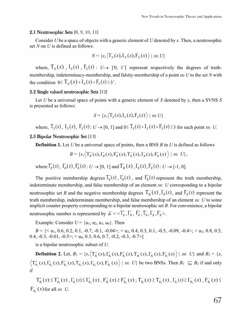
2.1 Neutrosophic Sets [8, 9, 10, 11]

Consider U be a space of objects with a generic element of U denoted by x. Then, a neutrosophic set N on U is defined as follows:

N = {x, )(F),(I),(T xxx NNN xU}

where, )(T xN , )(I xN , )(F xN : U ]-0, 1+[ represent respectively the degrees of truth-membership, indeterminacy-membership, and falsity-membership of a point xU to the set N with the condition -0 )(T xN + )(I xN + )(F xN 3+.

2.2 Single valued neutrosophic Sets [12]

Let U be a universal space of points with a generic element of X denoted by x, then a SVNS S is presented as follows:

S = {x, )(F),(I),(T xxx SSS xU}

where, )(T xS , )(I xS , )(F xS : U [0, 1] and 0 )(T xS + )(I xS + )(F xS 3 for each point x U.

2.3 Bipolar Neutrosophic Set [13]

Definition 1. Let U be a universal space of points, then a BNS B in U is defined as follows

B = {x, )(F ),(I ),(T),(F),(I),(T xxxxxx BBBBBB x U},

where )(T xB , )(I xB

, )(F xB : U [0, 1] and )(T xB

, )(I xB , )(F xB

: U [-1, 0].

The positive membership degrees )(T xB , )(I xB

, and )(F xB represent the truth membership,

indeterminate membership, and false membership of an element x U corresponding to a bipolar neutrosophic set B and the negative membership degrees )(T xB

, )(I xB , and )(F xB

represent the truth membership, indeterminate membership, and false membership of an element x U to some implicit counter property corresponding to a bipolar neutrosophic set B. For convenience, a bipolar neutrosophic number is represented by b~ = <

BT ,

BI ,

BF ,

BT ,

BI ,

BF >.

Example: Consider U = {u1, u2, u3, u4}. Then

B = {< u1, 0.6, 0.2, 0.1, -0.7, -0.1, -0.04>; < u2, 0.4, 0.3, 0.1, -0.5, -0.09, -0.4>; < u3, 0.8, 0.5, 0.4, -0.3, -0.01, -0.5>; < u4, 0.3, 0.6, 0.7, -0.2, -0.3, -0.7>]

is a bipolar neutrosophic subset of U.

Definition 2. Let, B1 = {x, )(F ),(I ),(T),(F),(I),(T111111

xxxxxx BBBBBB x U} and B2 = {x,

)(F ),(I ),(T),(F),(I),(T222222

xxxxxx BBBBBB x U} be two BNSs. Then B1 B2 if and only

if

)(T1

xB )(T

2xB

, )(I1

xB )(I

2xB

, )(F1

xB )(F

2xB

; )(T1

xB )(T

2xB

, )(I1

xB )(I

2xB

, )(F1

xB

)(F2

xB for all x U.


68

Definition 3. Consider, B1 = {x, )(F ),(I ),(T),(F),(I),(T111111

xxxxxx BBBBBB x U} and B2 =

{x, )(F ),(I ),(T),(F),(I),(T222222

xxxxxx BBBBBB x U} be two BNSs. Then B1 = B2 if and only

if

)(T1

xB = )(T

2xB

, )(I1

xB = )(I

2xB

, )(F1

xB = )(F

2xB

; )(T1

xB = )(T

2xB

, )(I1

xB = )(I

2xB

, )(F1

xB =

)(F2

xB for all x U.

Definition 4.Consider, B = {x, )(F ),(I ),(T),(F),(I),(T xxxxxx BBBBBB x U} be a BNS.

The complement of B is denoted by Bc and is defined by

)(T c xB = {1+} - )(T xB

, )(I c xB = {1+} - )(I xB

, )(F c xB = {1+} - )(F xB

;

)(T c xB = {1-} - )(T xB

, )(I c xB = {1-} - )(I xB

, )(F c xB = {1-} - )(F xB

for all x U.



{x, )(F ),(I ),(T),(F),(I),(T222222

xxxxxx BBBBBB x U} be two BNSs. Then their union B1B2

is defined as follows:

B1 B2 = {Max ( )(T1

xB , )(T

2xB

),2

)(I)(I21

xx BB

, Min ( )(F1

xB , )(F

2xB

), Min ( )(T1

xB ,

)(T2

xB ),

2)(I)(I

21xx BB

, Max ( )(F

1xB

, )(F2

xB )} for all x U.



{x, )(F ),(I ),(T),(F),(I),(T222222

xxxxxx BBBBBB x U} be two BNSs. Then their intersection B1

B2 is defined as follows:

B1 B2 = {Min ( )(T1

xB , )(T

2xB

),2

)(I)(I21

xx BB

, Max ( )(F1

xB , )(F

2xB

), Max ( )(T1

xB ,

)(T2

xB ),

2)(I)(I

21xx BB

, Min ( )(F

1xB

, )(F2

xB )}for all x U.

Definition 7. Suppose 1~b = <

1TB ,

1I B ,

1FB ,

1TB ,

1I B ,

1FB > and 2

~b = <

2TB ,

2I B ,

2FB ,

2TB ,

2I B ,

2FB > are

two BNNs, then

i. α . 1~b = <1 – (1 -

1TB ) α , (

1I B ) α , (

1FB ) α , - (-

1TB ) α , - (-

1I B ) α , - (1 – (1 – (-

1FB )) α )>;

ii. ( 1~b ) α = < (

1TB ) α , 1 - (1 -

1I B ) α , 1 - (1 -

1FB ) α , - (1 – (1 – (-

1TB )) α ), - (-

1I B ) α , – (-

1FB )) α )>;

iii. 1~b + 2

~b = <

1TB +

2TB -

1TB .

2TB ,

1I B .

2I B ,

1FB .

2FB , -

1TB .

2TB , - (-

1I B -

2I B -

1I B .

2I B ), - (-

1FB -

2FB -

1FB .

2FB )>;


69

iv. 1~b . 2

~b = <

1TB .

2TB ,

1I B +

2I B -

1I B .

2I B ,

1FB +

2FB -

1FB .

2FB , (-

1TB -

2TB -

1TB .

2TB ), -

1I B .

2I B , -

1FB .

2FB )>,

where α > 0. 2.4. The distance between two BNNs

In this sub-section, we propose the distance between two BNNs.

Consider 1B =

m

1i(xi, <

1TB (xi),

1I B (xi),

1FB (xi),

1TB (xi),

1I B (xi),

1FB (xi)>) , 2B =

m

1i(xi, <

2TB (xi),

2I B

(xi),

2FB (xi),

2TB (xi),

2I B (xi),

2FB (xi)>) be two BNNs then,

(1). The Hamming distance between two BNNs is defined as follows:

DH ( 1B , 2B ) =

m

1i{|(

1TB (xi) -

2TB (xi))| + |(

1I B (xi) -

2I B (xi))| + |(

1FB (xi) -

2FB (xi))| + |(

1TB (xi)-

2TB (xi))|

+ |(

1I B (xi) -

2I B (xi))| + |(

1FB (xi) -

2FB (xi))|} (1)

(2). The normalized Hamming distance between two BNNs is defined as follows:

NDH ( 1B , 2B ) = m61

m

1i{|(

iBT (xi) -

2TB (xi))| + |(

1I B (xi) -

2I B (xi))| + |(

1FB (xi) -

2FB (xi))| + |(

1TB (xi) -

2TB (xi))| + |(

1I B (xi) -

2I B (xi))| + |(

1FB (xi) -

2FB (xi))|} (2)

(3). The Euclidean distance between two BNNs is defined as follows:

EH ( 1B , 2B ) =

m

i 2ii

2ii

2ii

2ii

2ii

2ii

))(F)(F())(I)(I())(T)(T(

))(F)(F())(I)(I())(T)(T(

212121

212121

xxxxxx

xxxxxx

BBBBBB

BBBBBB

(3)

(4). The normalized Euclidean distance between two BNNs is defined as follows:

NEH ( 1B , 2B ) =

m

i 2ii

2ii

2ii

2ii

2ii

2ii

))(F)(F())(I)(I())(T)(T(

))(F)(F())(I)(I())(T)(T(

6m1

212121

212121

xxxxxx

xxxxxx

BBBBBB

BBBBBB

(4)

with the following properties:

(1). 0DH ( 1B , 2B )6m

(2). 0 NDH ( 1B , 2B ) 1

(3). 0 EH ( 1B , 2B ) 6m

(4). 0 NEH ( 1B , 2B ) 1.

3. TOPSIS method for MADM with bipolar neutrosophic information

In this Section, we present an approach based on TOPSIS method to deal with MADM problems under bipolar neutrosophic environment.


70

Let A = {A1, A2, …, Am}, (m 2) be a discrete set of m feasible alternatives, C = {C1, C2, …, Cn}, (n 2) be a set of attributes under consideration and w = (w1, w2, …, wn)T be the unknown

weight vector of the attributes with 0wj1 and

n

1j jw = 1. The rating of performance value of

alternative Ai, (i = 1, 2, …, m) with respect to the predefined attribute Cj, (j = 1, 2, …, n) is presented by the decision maker (DM) and they can be expressed by BNNs. Therefore, the proposed approach is presented using the following steps:

Step 1. Construction of decision matrix with BNNs The rating of performance value of alternative Ai (i = 1, 2, …, m) with respect to the attribute

Cj, (j = 1, 2, …, n) is expressed by BNNs and they can be presented in the decision matrix as follows:

nmijr~

=

mnm2m1

2n2221

1n1211

r...rr............r...rrr...rr

Here, we have rij = (

ijT ,

ijI ,

ijF ,

ijT ,

ijI ,

ijF ) with

ijT ,

ijI ,

ijF , -

ijT , -

ijI , -

ijF [0, 1] and 0

ijT +

ijI +

ijF -

ijT -

ijI -

ijF 6 for i = 1, 2, …, m; j = 1, 2, …, n.

Step 2. Determination of weights of the attributes We assume that the weights of the attributes are not equal and they are fully unknown to the

DM. Therefore, in this paper, maximizing deviation method [24] is used to find the unknown weights. The main idea of maximizing deviation method can be expressed as follows. If the attribute values rij (j = 1, 2, …, n) in the attribute Cj have small differences between the alternatives, then Cj has a small significance in ranking of all alternatives and a small weight is assigned for the attribute. If the attribute values rij (j = 1, 2, …, n) in the attribute Cj are same, then Cj has no effect in the ranking results and zero is assigned to the weight of the attribute. However, if the attribute values rij (j = 1, 2, …, n) over the attribute Cj have big differences, then Cj will play a key role in ranking of all alternatives and we will allocate a big weight for the attribute. The deviation values of alternative Ai (i = 1, 2, …, m) to all other alternatives under the attribute Cj (j = 1, 2, …, n) can

be defined as Zij (wj) = jkjm

1k ij )wr,(rz

, then Zj (wj) = jm

1i ijwZ

= jkj

m

1i

m

1kij )wr,(rz

presents the total

deviation values of all alternatives to the other alternatives for the attribute Cj (j = 1, 2, …, n). Now

Z (wj) = )w(Z jn

1j j

= jkjm

1i

m

1k ijn

1j)wr,(rz

presents the total deviation of all attributes to the other

alternatives with respect to all alternatives. Now we construct the non-linear optimizing model based on above analysis to obtain unknown attribute weight wj as follows:

Max Z (wj) = jkjm

1i

m

1k ijn

1j)wr,(rz

(5)

Subject to

n

1j

2jw = 1, wj 0, j = 1, 2, …, n.


71

We now formulate the Lagrange multiplier function, and obtain

L (wj, ρ ) = jkjm

1i

m

1k ijn

1jw)r,(rz

+ρ (

q

1j

2jw -1)

whereρ is the Lagrange multiplier.

Then, we calculate the partial derivatives of L with respect to wj andρ respectively as follows:

j

j

wρ),(wL

= jkj

m

1i

m

1k ij w)r,(rz

+ρ (

n

1j

2jw -1) = 0,

ρρ),(wL j

=

n

1j

2jw -1 = 0.

Therefore, the weight of the attribute Cj is obtained as

wj =

n

1j

2

kjm

1i

m

1k ij

kjm

1i

m

1k ij

)r,(rz

)r,(rz

(6)

and the normalized weight of the attribute Cj is given by

*jw =

n

1j kjm

1i

m

1k ij

kjm

1i

m

1k ij

)r,(rz

)r,(rz

. (7)

Step 3. Construction of weighted decision matrix We find aggregated weighted decision matrix by multiplying weights [25] of the attributes and

the aggregated decision matrixnm

wij

jr

is constructed as follows:

nmijr wj =

nm

wij

jr

=

n21

n21

n21

wmn

wm2

wm1

w2n

w22

w21

w1n

w12

w11

r...rr............r...rr

r...rr

jwijr = ( jw

ijT , jwijI , jw

ijF , jwijT , jw

ijI , jwijF ) with w

ijT , wijI , w

ijF , wijT , w

ijI , wijF [0, 1] and 0

wijT + w

ijI + wijF - w

ijT - wijI - w

ijF 6 for i = 1, 2, …, m; j = 1, 2, …, n.

Step 4. Identify the bipolar neutrosophic relative positive ideal solution (BNRPIS) and bipolar neutrosophic relative negative ideal solution (BNRNIS)

In real life decision making, we confront two types of attributes namely, benefit type attributes ( 1β ) and cost type attributes ( 2β ). In bipolar neutrosophic environment, assume that w

BNRPISQ and


72

wBNRNISQ be the bipolar neutrosophic relative positive ideal solution (BNRPIS) and bipolar

neutrosophic relative negative ideal solution (BNRNIS). Then, wBNRPISQ and w

BNRNISQ are defined as follows:

wBNRPISQ =( ,F,I,T,F,I,T 111111 w

1w1

w1

w1

w1

w1

, 222222 w2

w2

w2

w2

w2

w2 F,I,T,F,I,T ,…,

nnnnnn wn

wn

wn

wn

wn

wn F,I,T,F,I,T ) (8)

wBNRNISQ = ( ,F,I,T,,-FI,T 111111 w

1w1

w1

w1

w1

w1

, 222222 w2

w2

w2

w2

w2

w2 F,I,T,F,I,T , …,

nnnnnn wn

wn

wn

wn

wn

wn F,I,T,F,I,T ) (9)

where jjjjjj w

jwj

wj

wj

wj

wj F,I,T,F,I,T = <[{ )(TMax jw

iji

|j 1β }; { )(TMin jwiji

|j 2β }],

[{ )(IMin jwiji

| j 1β }; { )(IMax jwiji

|j 2β }], [{ )(FMin jwiji

|j 1β }; { )(FMax jwij

i

|j 2β }],

[{ )(TMin jwiji

|j 1β }; { )(TMax jwij

i

|j 2β }], [{ )(IMax jw

iji

|j 1β }; { )(IMin jwiji

|j

2β }],[{ )(FMax jwiji

|j 1β }; { )(FMin jwiji

|j 2β }]>, j = 1, 2, …, n;

jjjjjj wj

wj

wj

wj

wj

wj F,I,T,F,I,T = < [{ )(TMin jw

iji

|j 1β }; { )(TMax jwiji

|j 2β }],

[{ )(IMax jwiji

| j 1β }; { )(IMin jwiji

| j 2β }], [{ )(FMax jwiji

|j 1β }; { )(FMin jwij

i

|j 2β }],

[{ )(TMax jwiji

|j 1β }; { )(TMin jwij

i

|j 2β }], [{ )(IMin jw

iji

|j 1β }; { )(IMax jwiji

|j 2β }],

[{ )(FMin jwiji

|j 1β }; { )(FMax jwiji

|j 2β }] >, j = 1, 2, …, n.

Step 5. Calculation of distance of each alternative from BNRPIS and BNRNIS

The normalized Euclidean distance of each alternative jjjjjj wij

wij

wij

wij

wij

wij F,I,T,F,I,T from

the BNRPIS jjjjjjjjjjjj F,I,T,F,I,T wwwwww for i = 1, 2, …, m; j = 1, 2, …., n can be

defined as follows:

iNEuc =

n

1j 2wij

wij

2wij

wij

2wij

wij

2wij

wij

2wij

wij

2wij

wij

)FF()II()TT

)FF()II()TT(

6n1

jjjjjj

jjjjjj

(10)

Similarly, normalized Euclidean distance of each alternative jjjjjj w

ijwij

wij

wij

wij

wij F,I,T,F,I,T

from the BNRNIS jjjjjj wj

wj

wj

wj

wj

wj F,I,T,F,I,T for i = 1, 2, …, m; j = 1, 2, …., n can be

written as follows:


73

iNEuc =

n

1j 2wij

wij

2wij

wij

2wij

wij

2wij

wij

2wij

wij

2wij

wij

)FF()II()TT

)FF()II()TT(

6n1

jjjjjj

jjjjjj

(11)

Step 6. Evaluate the relative closeness co-efficient The relative closeness co-efficient of each alternative Ai, (i = 1, 2, …, m) with respect to the

BNRPIS wBNRPISQ is defined as follows:

*icc =

iN

iN

iN

EucEucEuc

(12)

where, 0*icc 1, i = 1, 2, …, m.

Step 7. Rank the alternatives Rank the alternatives according to the descending order of the alternatives and select the best

alternative with maximum value of *icc .

4. A numerical example

We consider the problem [13] where a customer wants to buy a car. There are four types cars (alternatives) Ai, i = 1, 2, 3, 4 are available. The customer considers four attributes namely Fuel economy (C1), Aerod (C2), Comfort (C3), Safety C4 to assess the alternatives. Now we solve the problem with bipolar neutrosophic information based on TOPSIS method to select most desirable car for the customer. Then, the proposed TOPSIS approach for solving the problem is presented in the following steps:

Step 1: Formulation of decision matrix We construct the decision matrix with bipolar neutrosophic information presented by the DM

as given below (see Table 1).

Table 1. The decision matrix provided by the DM

C1 C2 C3 C4

A1 (0.5, 0.7, 0.2, -0.7, -0.3, -0.6) (0.4, 0.4, 0.5, -0.7, -0.8, -0.4) (0.7, 0.7, 0.5, -0.8, -0.7, -0.6) (0.1, 0.5, 0.7, -0.5, -0.2, -0.8)

A2 (0.9, 0.7, 0.5, -0.7, -0.7, -0.1) (0.7, 0.6, 0.8, -0.7, -0.5, -0.1) (0.9, 0.4, 0.6, -0.1, -0.7, -0.5) (0.5, 0.2, 0.7, -0.5, -0.1, -0.9)

A3 (0.3, 0.4, 0.2, -0.6, -0.3, -0.7) (0.2, 0.2, 0.2, -0.4, -0.7, -0.4) (0.9, 0.5, 0.5, -0.6, -0.5, -0.2) (0.7, 0.5, 0.3, -0.4, -0.2, -0.2)

A4 (0.9, 0.7, 0.2, -0.8, -0.6, -0.1) (0.3, 0.5, 0.2, -0.5, -0.5, -0.2) (0.5, 0.4, 0.5, -0.1, -0.7, -0.2) (0.4, 0.2, 0.8, -0.5, -0.5, -0.6)


74

Step 2. Calculation of the weights of the attributes We use normalized Hamming distance and obtain the weights of the attributes by maximizing

deviation method as follows:

w1 = 0.2585, w2 = 0.2552, w3 = 0.2278, w4 = 0.2585, where

4

1j jw = 1.

Step 3. Construction of weighted decision matrix The weighted decision matrix is obtained by multiplying weights to decision matrix as given

below (see Table 2)

Table 2. The weighted decision matrix

C1 C2 C3

A1 (0.164, 0.912, 0.66, -0.912, -0.732, -0.211) (0.122, 0.791, 0.838, -0.913, -0.945, -0.122) (0.24, 0.922, 0.854, -0.95, -0.922, -0.208)

A2 (0.488, 0.912, 0.836, -0.912, -0.912, -0.027) (0.264, 0.874, 0.945, -0.913, -0.838, -0.026) (0.408, 0.812, 0.89, -0.592, -0.922, -0.162) A3 (0.088, 0.789, 0.66, -0.876, -0.732, -0.267) (0.055, 0.663, 0.663, -0.791, -0.913, -0.122) (0.408, 0.854, 0.854, -0.89, -0.854, -0.055)

A4 (0.448, 0.912, 0.66, -0.944, -0.876, -0.027) (0.087, 0.838, 0.663, -0.838, -0.838, -0.055) (0.146, 0.812, 0.854, -0.592, -0.922, -0.055)

______________________________ C4

______________________________ A1 (0.027, 0.836, 0.912, -0.836, -0.66, -0.337) A2 (0.164, 0.66, 0.912, -0.836, -0.551, -0.444) A3 (0.267, 0.836, 0.088, -0.789, -0.66, -0.055) A4 (0.124, 0.66, 0.944, -0.836, -0.836, -0.208)

_______________________________

Step 4. Recognize the BNRPIS and BNRNIS

The BNRPIS ( wBPRPISR ) and BNRNIS ( w

BPRNISR ) are obtained from the weighted decision matrix as follows:

wBPRPISR = < (0.448, 0.789, 0.66, -0.944, -0.732, -0.027); (0.264, 0.663, 0.663, -0.913, -0.838, -

0.026); (0.408, 0.812, 0.854, -0.89, -0.854, -0.055); (0.267, 0.66, 0.88, -0.836, -0.551, -0.055) >; w

BPRNISR = < (0.088, 0.912, 0.836, -0.876, -0.912, -0.267); (0.055, 0.878, 0.945, -0.791, -0.945, -0.122); (0.146, 0.922, 0.89, -0.592, -0.922, -0.208); (0.027, 0.836, 0.912, -0.789, -0.836, -0.444) >.

Step 5. Distance measures of each alternative from the BNRPISs and BNRNISs


75

The normalized Euclidean distances of each alternative from the BNRPISs are computed as follows:

1NEuc = 0.0479, 2

NEuc = 0.0161, 3NEuc = 0.013, 4

NEuc = 0.0469.

Similarly, the normalized Euclidean distances of each alternative from the BNRNISs are computed as follows:

1NEuc = 0.0123, 2

NEuc = 0.0247, 3NEuc = 0.0548, 4

NEuc = 0.0192.

Step 6. Calculation of the relative closeness coefficient

We determine the relative closeness co-efficient *icc , (i = 1, 2, 3, 4) using Eq. (12).

*1cc = 0.2043, *

2cc = 0.6054, *3cc = 0.8082, *

4cc = 0.2905.

Step 7. Rank the alternatives

The ranking order of the cars is presented according to the relative closeness coefficient as given below.

A3 A2 A4 A1 Consequently, A3 is the most preferable alternative.

Note 1: Deli et al. [13] consider the weight vector of the attributes as w = (21 ,

41 ,

81 ,

81 ) for

car selection. However, if we take weight vector of the attributes as w = (21 ,

41 ,

81 ,

81 ), then

relative closeness co-efficient *icc , (i = 1, 2, 3, 4) are computed as given below.

*1cc = 0.3746, *

2cc = 0.5761, *3cc = 0.4716, *

4cc = 0.6944.

Therefore, the ranking order of the cars can be represented as follows:

A4 A2 A3 A1 So, A4 would be the most suitable alternative.

5. Conclusion

In this paper, we present a TOPSIS method for solving MADM problem with bipolar neutrosophic information. We define Hamming distance function and Euclidean distance function to determine the distance between BNNs. In the decision making situation, the rating of performance values of the alternatives with respect to the attributes are provided by the DM in terms of BNNs. The weights of the attributes are obtained by maximizing deviation method and we construct the weighted decision matrix. We also define BNRPIS and BNRNIS. Euclidean distance measure is employed to compute the distances of each alternative from BNRPISs as well as BNRNISs. Relative closeness coefficients are calculated to rank the alternative and to obtain the best alternative. Finally, the proposed method is applied to solve a car selection problem to verify the applicability of the proposed method and comparison with other existing method is also provided.


76

References 1. L.A. Zadeh. Fuzzy sets, Information and Control, 8 (1965), 338-353. 2. I.B.Turksen. Interval valued fuzzy sets based on normal forms, Fuzzy Sets and Systems, 20(2) (1986),

191-210. 3. K.T. Atanassov. Intuitionistic fuzzy sets, Fuzzy Sets and Systems, 20 (1986), 87-96. 4. K.M. Lee. Bipolar-valued fuzzy sets and their operations, In Proc. Int. Conf. on Intelligent Technologies,

Bangkok, Thailand (2000), 307-312. 5. K.M. Lee. Bipolar fuzzy subalgebras and bipolar fuzzy ideals of BCK/BCI- algebras, Bull. Malays. Math.

Sci. Soc., 32(3) (2009), 361-367. 6. J. Chen, S. Li, M. Ma, X. Wang. m-Polar fuzzy sets: an extension of bipolar fuzzy sets, The Scientific

World Journal, 2014. http://dx.doi.org/10.1155/2014/416530. 7. M. Zhou, S. Li. Application of bipolar fuzzy sets in semirings, Journal of Mathematical Research with

Applications, 34(1) (2014), 61-72. 8. F. Smarandache. A unifying field of logics. Neutrosophy: neutrosophic probability, set and logic,

American Research Press, Rehoboth, 1998. 9. F. Smarandache. Linguistic paradoxes and tautologies. Libertas Mathematica, University of Texas at

Arlington, IX (1999), 143-154. 10. F. Smarandache. Neutrosophic set – a generalization of intuitionistic fuzzy sets, International Journal of

Pure and Applied Mathematics, 24(3) (2005), 287-297. 11. F. Smarandache. Neutrosophic set – a generalization of intuitionistic fuzzy set, Journal of Defence

Resources Management, 1(1) (2010), 107-116. 12. H. Wang, F. Smarandache, Y. Zhang, and R. Sunderraman. Single valued neutrosophic sets, Multi-space

and Multi-Structure, 4 (2010), 410-413. 13. Deli, M. Ali, F. Smarandache. Bipolar neutrosophic sets and their application based on multi-criteria

decision making problems, Proceedings of the 2015 International Conference on Advanced Mechatronic Systems, Beiging, China, August, 20-24, 2015, 249-254.

14. S. Pramanik, K.Mondal. Rough bipolar neutrosophic set. Global Journal of Engineering Science and Research Management 3(6) (2016), 71-81.

15. Z. Zhang, C. Wu. A novel method for single-valued neutrosophic multi-criteria decision making with incomplete weight information, Neutrosophic Sets and Systems, 4 (2014), 35-49.

16. C.L. Hwang, K. Yoon. Multiple attribute decision making: methods and applications, Springer, New York, 1981.

17. P. Chi, P. Liu. An extended TOPSIS method for the multiple attribute decision making problems based on interval neutrosophic set, Neutrosophic Sets and Systems, 1 (2013), 63-70.

18. P. Biswas, S. Pramanik, B.C. Giri. TOPSIS method for multi-attribute group decision making under single-valued neutrosophic environment, Neural Computing and Applications, (2015), DOI: 10.1007/s00521-015-1891-2.

19. S. Broumi, J. Ye. F. Smnarandache. An extended TOPSIS method for multiple attribute decision making based on interval neutrosophic uncertain linguistic variables. Neutrosophic Sets and Systems 8 (2015), 22-31.

20. S. Pramanik, P. P. Dey, B. C. Giri. TOPSIS for singled valued soft expert set based multi-attribute decision making problems. Neutrosophic Sets and Systems 10 (2015), 88-95.

21. P.P. Dey, S. Pramanik, B.C. Giri. Generalized neutrosophic soft multi-attribute group decision making based on TOPSIS. Critical Review 11 (2015), 41-55.

22. K. Mondal, S. Pramanik, F. Smarandache. TOPSIS in rough neutrosophic environment. Neutrosophic Sets and Systems 13 (2016). In Press.


77

23. V. Uluçay, I. Deli, M. Şahin, Similarity measures of bipolar neutrosophic sets and their application to multiple criteria decision making. Neural Computing and Applications (2016). doi 10.1007/s00521-016-2479-1.

24. Y.M. Yang. Using the method of maximizing deviations to make decison for multi-indices, System Engineering and Electronics, 7 (1998) 24-31.

25. J.J. Peng, J.Q. Wang, J. Wang, H. Zhang, X. Chen. Simplified neutrosophic sets and their applications in multi-criteria group decision-making problems, International Journal of Systems Science, (2014), DOI:10.1080/00207721.2014.994050.

topsis for solving multi-attribute decision making...

Documents