tools for quantifying isotopic niche space and dietary variation at …. mammal. 2012...

Tools for quantifying isotopic niche space and dietary variation at theindividual and population level

SETH D. NEWSOME,* JUSTIN D. YEAKEL, PATRICK V. WHEATLEY, AND M. TIM TINKER

Department of Zoology and Physiology, University of Wyoming, 1000 East University Avenue, Department 3166,Laramie, WY 82071, USA (SDN)Department of Ecology and Evolutionary Biology, University of California–Santa Cruz, Santa Cruz, CA 95064, USA(JDY)Center for Isotope Geochemistry, Lawrence Berkeley National Laboratory, 1 Cyclotron Road, MS 70A-4418, Berkeley,CA 94720, USA (PVW)United States Geological Survey, Western Ecological Research Center, Long Marine Laboratory, 100 Shaffer Road,Santa Cruz, CA 95060, USA (MTT)

* Correspondent: [email protected]

Ecologists are increasingly using stable isotope analysis to inform questions about variation in resource andhabitat use from the individual to community level. In this study we investigate data sets from 2 California seaotter (Enhydra lutris nereis) populations to illustrate the advantages and potential pitfalls of applying variousstatistical and quantitative approaches to isotopic data. We have subdivided these tools, or metrics, into 3categories: IsoSpace metrics, stable isotope mixing models, and DietSpace metrics. IsoSpace metrics are used toquantify the spatial attributes of isotopic data that are typically presented in bivariate (e.g., d13C versus d15N) 2-dimensional space. We review IsoSpace metrics currently in use and present a technique by which uncertaintycan be included to calculate the convex hull area of consumers or prey, or both. We then apply a Bayesian-basedmixing model to quantify the proportion of potential dietary sources to the diet of each sea otter population andcompare this to observational foraging data. Finally, we assess individual dietary specialization by comparing apreviously published technique, variance components analysis, to 2 novel DietSpace metrics that are based onmixing model output. As the use of stable isotope analysis in ecology continues to grow, the field will need a setof quantitative tools for assessing isotopic variance at the individual to community level. Along with recentadvances in Bayesian-based mixing models, we hope that the IsoSpace and DietSpace metrics described herewill provide another set of interpretive tools for ecologists.

Key words: isotope mixing models, isotopic niches, sea otters, stable isotope analysis

E 2012 American Society of Mammalogists

DOI: 10.1644/11-MAMM-S-187.1

Stable isotope analysis has rapidly transitioned from a noveltechnique of limited interest to one of the most valuable toolsin an ecologist’s tool set, and the number of published papersthat utilize isotopic approaches is growing at an exponentialrate. Stable isotope analysis has been adopted by nearly everysubdiscipline of ecology because it allows scientists to traceresources within and between animals, plants, and microbes, atscales ranging from the individual to the community level.Recent reviews of the subject summarize how isotopic datacan be used to evaluate information on resource or habitat use,or both, that would help define an organism’s niche in atraditional Grinnellian (Grinnell 1917), Eltonian (Elton 1927),or Hutchinsonian (Hutchinson 1957) sense. Some have evengone so far as to utilize the term isotopic niche (Flaherty and

Ben-David 2010; Martınez del Rio et al. 2009a; Newsome etal. 2007) because isotopic axes provide information on thebionomic and scenopoetic aspects of the niche (Hutchinson1978) and arguably can be as informative as many otherenvironmental variables traditionally used to define nichehypervolumes. A clear distinction, however, must be madebetween the isotopic and realized niche space. Only with theconversion of isotopic data to numerical estimates of resourceor habitat use, or both, via mixing models can traditional

w w w . m a m m a l o g y . o r g

Journal of Mammalogy, 93(2):329–341, 2012

329

www.mammalogy.org

components of an organism’s niche be evaluated with isotopictools.

As one might expect of a tool that was adopted quickly andwith little experimental groundwork, there are a number ofunresolved issues concerning the use of stable isotopes asintrinsic ecological tools. In general, these issues centeraround ecophysiological and methodological considerationsthat in some (but not all) cases can have a major effect on howstable isotope data are interpreted. For example, a recent waveof controlled feeding experiments examined isotopic incorpo-ration (or turnover) rates for a wide variety of tissues andtaxonomic levels (Martınez del Rio et al. 2009b), which isessential for accurate interpretation of applied studies.Likewise, recent laboratory and field-based studies (Gaye-Siessegger et al. 2003; Newsome et al. 2010; Vander Zandenand Rasmussen 2001) have investigated potential mechanismsresponsible for variation in trophic discrimination factors, orthe difference in isotopic composition between a consumer’stissues and its diet (Dtissue2diet), that have important implica-tions for examining diet or trophic level, or both, ofindividuals or populations, which is the most common useof stable isotope analysis in ecology. Methodologicalconsiderations include sample pretreatment, such as the properpreparation of tissues for hydrogen isotope (dD) analysis(Bowen et al. 2005) and whether consumer and prey tissuesshould be lipid-extracted prior to carbon isotope (d13C)analysis (Newsome et al. 2010; Post 2002; Ricca et al.2007). As the use of stable isotope analysis in ecologycontinues to grow, these issues and others currently unrecog-nized, present substantial challenges to the research commu-nity. In our opinion, these challenges represent an intriguingopportunity because they transcend the disciplines of ecologyand physiology and require the need for both experimental andapplied work.

Another methodological issue concerns the question of howisotopic data should be treated from a statistical andinterpretive standpoint, which is quickly becoming a richsource of literature. Most of this work has focused on variousforms of stable isotope mixing models that can be used todetermine source proportions in consumer diets (Moore andSemmens 2008; Parnell et al. 2010; Phillips and Gregg 2003;Phillips and Koch 2002); on statistically based interpretationof dD data that is used to assess movement and migratorypatterns (Farmer et al. 2008; Wunder and Norris 2008); on theuse of single- versus multiple-compartment models forevaluating isotopic incorporation rates (Carleton et al. 2008;Cerling et al. 2007); and on the use of spatial metrics tocharacterize community-level variation in trophic structureacross space and time (Layman et al. 2007; Turner et al.2010). In this paper we address the 1st and 4th topics, andbriefly summarize here the various forms of mixing models,the utility of spatial metrics, and the type of information these2 approaches can provide; see the ‘‘Materials and Methods’’for a more detailed description.

Initially, mixing models used a linear framework todetermine a unique mathematical solution for the relative

contributions of n + 1 prey sources using n isotope systems(e.g., d13C or d15N, or both). Later iterations of these modelsallowed users to compensate for differences in elementalconcentrations among potential sources (Phillips and Koch2002), which have important implications for the interpreta-tion of isotopic data derived from omnivores that consumeresources of varying quality (i.e., nitrogen content). Forgeneralists that consume a wide variety of potential foodsources, however, these models were sometimes difficult touse in practice. In response, Phillips and Gregg (2003)produced IsoSource, which generates a frequency distributionof potential proportions for greater than n + 1 sources whenonly using n isotope systems. In the past few years, Bayesian-based models such as MixSIR (Moore and Semmens 2008)and SIAR (Parnell et al. 2010) have been developed that buildon the capabilities of IsoSource and allow users to includeinformation regarding isotopic variation in potential sourcesand trophic discrimination factors, as well as input priorinformation on resource or habitat use obtained from othertypes of data (e.g., scat analysis or observation).

Mixing models are useful tools for converting isotopic datainto a form that can be directly compared to traditionalecological information. In essence, these models provideestimates of trophic interaction strengths, or interactiondistributions in the case of IsoSource or Bayesian-basedapproaches, between consumers and their prey, and thereforehave greater ecological traction than comparisons of isotopicdata presented in 2-dimensional bivariate space (e.g., d13Cversus d15N). But even Bayesian-based mixing models can becumbersome, especially when applied to generalist specieswith diverse diets, in situations with an even distribution ofresources in the isotopic mixing space, or when makingcommunity-level comparisons of isotopic variation amongconsumers. In response, ecologists have started using spatialmetrics to quantify various aspects of their data in the bivariated13C versus d15N framework that is often used to presentisotopic data (Layman et al. 2007, in press; Turner et al. 2010).Spatial metrics were originally used by paleontologists tostudy the evolution of morphospace in the fossil record (Foote1990; Gould 1991), but were quickly adopted by ecologists toquantify differences in form and function among extant groupsin an evolutionary context (Watters 1991; Winemiller 1991).

A recent concept paper by Layman et al. (2007) focused onhow various spatial metrics, including convex hull area(CHA), nearest-neighbor distance (NND), and distance tocentroid (DC) can be used to quantify community-widemeasures of trophic structure. For example, the CHA of d13Cand d15N values in bivariate space for a population (or species)can provide an estimate of dietary diversity; see the‘‘Materials and Methods’’ for detailed descriptions of howthese metrics are calculated and the kind of information theyprovide. A sharp critique of this approach (Hoeinghaus andZeug 2008) highlighted the need to control for isotopicvariation among potential sources available to consumers thatoccupy different habitats (Matthews and Mazumder 2004) andconcluded that the conversion of isotopic data into source

330 JOURNAL OF MAMMALOGY Vol. 93, No. 2

proportions via mixing models was the best way to addressthis problem (Newsome et al. 2007).

Here we show that when properly applied, spatial metricsare an intuitive set of tools for evaluating dietary variation,trophic structure, and habitat use at not only the level of thecommunity, but also at the population and individual scale.We draw on existing spatial metrics, which we call IsoSpacemetrics, and offer ways in which these approaches can controlfor isotopic variation among sources. We also offer a fewnovel dietary metrics, which we call DietSpace metrics, thatare useful for assessing dietary specialization and comple-mentary to other approaches used in the literature (e.g.,variance components analysis). Our paper utilizes publishedisotopic data sets for 2 California sea otter (Enhydra lutrisnereis) populations (Newsome et al. 2009, 2010) to highlightboth the advantages and caveats of using these tools tointerpret isotopic data. Although the sea otter data sets areparticularly useful examples because they are paired withextensive observational data on diet composition, the toolsdescribed here could easily be applied to isotopic data fromother taxonomic groups, including microbes and plants.

MATERIALS AND METHODS

IsoSpace metrics.—Insight into isotopic systems can begained with the use of metrics that quantify aspects of isotopicbivariate space. IsoSpace is typically defined by d13C andd15N values of both the consumer and its potential resources(prey), and is often assumed to be equivalent to a consumer’sresource isotopic niche space (Martınez del Rio et al. 2009a;Newsome et al. 2007). Because isotopic values are normalizedto account for trophic discrimination, a consumer will fallwithin the isotopic space defined by those resources it hasconsumed (Fig. 1). The interior of this space is often referredto a prey or mixing space. Characteristics that are descriptiveof both ecological and environmental processes that underliethese isotopic values can be quantified by Euclideanmeasurements of the various shapes and distances within thisbivariate space. Although previous investigations haveestablished frameworks for evaluating consumer-level differ-ences when the isotopic values of resources do not change(Turner et al. 2010), such approaches have not incorporatedisotopic variance in potential prey available to differentpopulations that occupy different food webs. Here we brieflydescribe these measurements, as well as procedures by whichvariance can be incorporated. In contrast to a mixing modelapproach, note that consumer isotopic data do not have to betrophic-corrected prior to the calculation of the spatial metricsdescribed below.

The CHA is the simplest area that can be drawn around theoutermost coordinates that define the mixing space; interiorsources are excluded and will not be referred to here. Amixing space can be subdivided into a series of triangularcomponents (Fig. 1). The CHA can be calculated by the sumof the triangular areas within the convex hull; triangles aredrawn between a single arbitrary source and each pair of

nearest-neighbor sources that define the remaining hull. Ifvectors are labeled clockwise (P0–P5 in Fig. 1) the CHA canbe calculated:

CHA~1

2

Xn{1

i~1

ni|niz1j j, ð1Þ

where ni and ni + 1 are vectors defined as in Fig. 1, and |ni 3

ni + 1| is the magnitude of the cross product of the 2 vectors(equation 1). Because potential sources in IsoSpace aretypically distributions of values, it is important to takevariance into account. Although more rigorous methods maybe employed, here we use a simple algorithm to incorporatesource variation into CHA measurements. To incorporatevariance into CHA measurements, coordinates are randomlychosen from each unique source distribution; from this seriesthe CHA is calculated. This process is iterated such that arepresentative sample of potential CHAs is quantified acrossall source distributions. For the mixing spaces that we evaluatehere, 1 3 105 iterations is sufficient to accurately calculate theCHA, although the number of iterations required increaseswith greater isotopic variability of the convex hull, whichincreases the number of potential hull shapes. In principle, theCHA can be extrapolated to more than 2 dimensions (i.e.,when using more than 2 isotopic tracers) such that themeasurement would define a hypervolume, although thisquickly becomes computationally expensive and is beyond the

FIG. 1.—Theoretical d13C and d15N bivariate mixing spaceshowing how a variety of spatial (IsoSpace) metrics are calculated.The convex hull area (CHA) is the simplest area that can be drawnaround the outermost coordinates (labeled P0–P5) that define themixing space; interior sources are excluded. The mixing space can besubdivided into a series of triangular components and calculated asthe sum of the triangular areas within the CHA. In this example, themixing space vectors for the prey are labeled i1–i5; triangles aredrawn between a single arbitrary source and each pair of nearest-neighbor sources that define the remaining hull. The nearest-neighbordistance (NND) is defined by the minimum Euclidean distancebetween an isotopic coordinate relative to all other coordinates in aset. In this example, the NNDs for consumers C1–C5 are denoted byblue lines. Lastly, the centroid for the prey sources P0–P6 is markedby a red diamond and red lines denote the distances from each prey.

April 2012 SPECIAL FEATURE—ISOTOPIC NICHE SPACE AND DIETARY VARIATION 331

scope of this paper. We limit our discussion to a 2-dimensionalIsoSpace for simplicity.

The NND is defined by the minimum Euclidean distancebetween an isotopic coordinate relative to all other coordinatesin a set. In the 2-dimensional IsoSpace defined above, acoordinate is defined by its d13C and d15N values. We notethat the Euclidean distance is not limited with respect to thenumber of isotopes (dimensions) that are used. NNDs can becalculated for a set of isotopic coordinates that compriseindividuals within a population of a single species, or acrossmultiple species. The NND provides information regarding theclustering of points within a set. If the NND of a set ofcoordinates has low variance, the isotopic values of a groupare distributed across IsoSpace homogeneously; if NNDvalues are highly variable, the set of isotopic values isheterogeneously distributed (e.g., clustered or overdispersed).

The DC metric is defined as the Euclidean distance betweenan isotopic coordinate and a predetermined central coordinate,or centroid. In IsoSpace, the centroid coordinate is defined bythe average of each respective isotopic tracer (e.g., d13C)across all sources. The distance of each source to the centroidprovides information regarding the distribution of data pointsin bivariate space. Similar to the NND measurement, lowvariance of the DC implies a convex hull that is more circularin 2-dimensional space, and data points are distributed alongthe periphery of the convex hull. High variance in DC andNND implies that data points are more evenly distributed inbivariate space. The relative distribution of sources (i.e., prey)in bivariate space also has implications for the use of nonlinearmixing models because they tend to produce more definedresults if potential sources lie on the periphery of the mixingspace (see below). For the above metrics, we used a Welch’s2-way t-test to assess whether differences in mean valuesbetween sites were statistically significant.

Stable isotope mixing models.—Mixing models are designedto determine the contributions of a given set of resources to aconsumer’s diet. Traditionally, such models have been limitedto linear approaches, where the number of potential sources(i.e., prey) must be less than or equal to the number of isotopictracers + 1; in such a situation, a unique analytical solutionalways exists. For example, a 3-source mixing space definedby 2 isotopic systems is given by the mass balance equations(equation 2):

d13Cm~P3

i~1

fid13Ci, d15Nm~

P3

i~1

fid15Ni, 1~

P3

i~1

fi, ð2Þ

where d13C and d15N are the respective isotopic values ofcarbon and nitrogen in d notation (where d 5 1,000[(Rsample/Rstandard) 2 1], and R 5 either 13C/12C or 15N/14N) for boththe mix (m; i.e., the consumer) and sources (i; i.e., theresources or prey), whereas fi denotes the contribution of eachsource i to the mix. When n 5 3, all proportional contributionscan be solved analytically because there are 3 equations and 3unknowns (Phillips et al. 2005).

Most ecological scenarios are more complex and involvemany more sources than the number of isotopic tracers utilized

in the study. In addition, there is both natural variability anderror associated with isotopic measurements that cannot beincluded in the above framework. To address these issues, anumerical approximation called IsoSource was developed todetermine proportional source contributions (Phillips andGregg 2003). These numerical tools allowed the range ofproportional contribution-to-diet values to be determined,even if the number of sources was larger than the number ofisotopic tracers + 1, where no unique mathematical solution ispossible. Other approaches, such as binning sources withsimilar isotopic values, can be utilized to further decrease thenumber of potential sources and increase the accuracy of theresults (Phillips et al. 2005; Ward et al. 2011). Importantly,although ranges of contribution-to-diet values can be calcu-lated with these numerical procedures, all values within theranges are equally likely, thereby limiting interpretations whenranges are large.

Bayesian isotope mixing models were developed to copewith many potential sources, the uncertainties inherent inisotopic measurements, and the incorporation of priorknowledge. This approach results in an accurate quantificationof the uncertainty that characterizes scenarios with many moresources than isotopic tracers being utilized, as well as bothmeasurement and discrimination uncertainty. As such, the useof a Bayesian framework results in true posterior probabilitydistributions of the potential contributions of each source to amix.

Current Bayesian mixing models employ a sampling-importance-resampling or Markov chain Monte Carlo ap-proach to determine the likelihood of potential sourcecontributions to a mix. In general, for each source, a randomproportional contribution vector is proposed (fq; where fielements in the vector fq sum to unity). From this proposedvector, the mean and standard deviation are calculated, and thelikelihood of the mixture, given these parameters, isdetermined:

L x mmj,ssj

!!" #

~ Pn

k~1Pn

j~1

1

ssj

ffiffiffiffiffiffi2pp exp {

xkj{mmj

" #2

2ss2j

2

64

3

75

8><

>:

9>=

>;, ð3Þ

where x represents the isotopic data describing the mix (avector where each element is a set of isotopic measurements ofthe consumer), xkj is the value of the jth isotope of the kth

element of the mix, j is the mean of jth isotope of the proposal,and j is the standard deviation of the jth isotope of the proposal(equation 3). The posterior probability is then calculated:

P fq xj% &

~L x fq

!!% &p fq

% &P

L x fq

!!% &p fq

% & , ð4Þ

where L(x|fq) is as described above, P(fq) is the probability ofthe given proposal based on prior information, and thedenominator is a normalizing constant (equation 4). Accordingto the sampling-importance-resampling or Markov chainMonte Carlo algorithms, proposals are generated randomly,and a given proposal is accepted if the unnormalized posterior


probability is higher than the previously proposed unnorma-lized posterior probability. As such, the most likely contribu-tion is iteratively approached across the likelihood space. Thefinal posterior probabilities are typically considered robust ifthere have been §1,000 accepted, unduplicated, contribution-to-diet proposals (see Moore and Semmens [2008] for details).The output of Bayesian isotope mixing models appears similarto the simulations of numerical linear models; however, theyare not equivalent. Values within a range given by Bayesianmixing models have associated probability densities, whereasvalues within the range given by linear mixing models all havethe same probability (i.e., a uniform distribution). Recentadvances in Bayesian mixing models have resulted inapproaches that assess hierarchies of isotopic data (e.g.,individuals within populations within species—Semmens etal. 2009), as well as sophisticated methods for binning sources(Ward et al. 2011).

For this study, we used previously published d13C and d15Ndata for 2 California sea otter (E. l. nereis) populations fromSan Nicolas Island (SNI) and Monterey Bay (MB) and theirrespective prey; see Newsome et al. (2009, 2010) for detailson sampling strategy, tissue pretreatment, and isotopicanalyses. Individual means and standard deviations werecalculated from the subsampled whisker segments for each seaotter. Trophic discrimination factors of 2.0% and 3.5% wereused for d13C and d15N, respectively (Newsome et al. 2010) inthe mixing models for the SNI population. For MB, we usedslightly different trophic discrimination factors of 2.5% and3.5% for d13C and d15N, respectively (Newsome et al. 2009).

IsoSpace metrics were assessed for both SNI and MB seaotters, as well as their potential prey. We then calculated theproportional contribution of each prey to the diets of SNI andMB sea otters at the individual level with the Bayesian isotopemixing model MixSIR. Because the multiple measurementsobtained from individual sea otter whiskers cannot beconsidered independent, a parameterized bootstrapping pro-cedure was employed to incorporate within-individual vari-ance into the model. By doing so, we were able to moreaccurately include variance associated with individual seaotter foraging behaviors while maintaining assumptionsintrinsic to the model. Posterior distributions for the SNI andMB sea otter populations were obtained by bootstrapping andpooling individual sea otter MixSIR results such that eachindividual contributed equally to the final posterior probabilitydistributions. Such an analysis can also be implemented with ahierarchical stable isotope mixing model (Semmens et al.2009).

DietSpace metrics.—In its simplest incarnation, a consum-er’s diet is represented as a vector f 5 (f1, f2, …, fn) , such thateach element of the vector (fi) represents the proportionalcontribution of a prey source (e.g., mixing model output), andn is the total number of prey. As stated previously, f must sumto unity. With the use of a Bayesian isotope mixing model, thediet of a consumer is defined by a posterior probabilitydistribution, represented by a series of numerically calculatedvectors, rather than a single vector. Accordingly, the

distribution of each source quantifies the error associatedwith the isotopic measurements of both the consumer and itsresources or the natural ecological variability of the consum-er’s diet, or both. Here we present a useful method by which tomeasure the degree of specialization for an individualconsumer and compare groups of consumers (or populations).Note that in this context we define ‘‘specialization’’ in theclassical sense of niche specialization, or the degree to which aconsumer relies on a subset of prey, with respect to the totalnumber of available prey, and distinguish this concept fromindividual diet specialization, which we discuss below.

The quantification of dietary specialization is particularlystraightforward if the source contribution-to-diet probabilitiesare known. Here we establish a dietary Euclidean space withas many dimensions as prey, and define the centroid as anultrageneralist consumer (Fig. 2A). For example, if a con-sumer’s diet consists of n prey items, the centroid would bedefined by the coordinate c 5 (1/n,1/n,1/n,1/n,1/n), such thatthe consumer is an ultrageneralist, where every preycontributes equally. By contrast, we define a 2nd point inthe Euclidean space that defines an ultraspecialist consumerby the coordinate w 5 (1,0,0,0,0), such that only 1 source isconsumed. We note that for this metric it does not matterwhich element of the coordinate w has a value of 1 (e.g.,(1,0,0,0,0) is equivalent to (0,1,0,0,0)). We can now define thedistance from the ultrageneralist centroid of a consumerrepresented by a particular dietary coordinate f, relative to anultraspecialist, and across all proposed contribution-to-dietvectors (equation 5), such that:

e~

ffiffiffiffiffiffiffiffiffiffiffiffiffiffiffiffiffiffiffiffiffiffiffiffiffiffiffiffiffiPni~1 fi{cið Þ2

q

ffiffiffiffiffiffiffiffiffiffiffiffiffiffiffiffiffiffiffiffiffiffiffiffiffiffiffiffiffiffiffiPni~1 wi{cið Þ2

q : ð5Þ

Thus the degree of dietary specialization at the populationlevel (e) varies between 0 and 1, where a value of 0 denotesthe ultrageneralist consumer and a value of 1 denotes theultraspecialist consumer (Fig. 2A). Because we have normal-ized this metric to the distance between the ultraspecialist andultrageneralist, it is comparable across consumers withdifferent numbers of potential prey, though it does notdistinguish between consumers that specialize on differentsubsets of prey. When the diet of a consumer is quantified byprobability distributions, e also will be defined by aprobability distribution, because each proposed dietary vectorhas an associated e value. Here we use this metric to analyzeoutput from a Bayesian isotope mixing model (MixSIR).Because mixing model results are expressed as a series ofcontribution to diet vectors, e can be calculated for each vectorindependently such that a distribution of e values is obtained.Furthermore, e values for individuals can be pooled to obtainniche specialization values for a population.

It is often convenient to compare the dietary habits of 2 ormore consumers, or an individual consumer with the meandietary habits of its population. Again we borrow a well-known relationship from linear algebra such that pairwisedietary comparisons can be easily made. We note that this and


similar metrics often have been used to compare species’niches and even dietary input, although, to our knowledge, ithas not been used in the context of isotopic data or mixingmodel output (Bolnick et al. 2002; Kohn and Riggs 1982;Smith et al. 1990; Tinker et al. 2008). Because a consumer’sdiet can be thought of as a unique vector in diet-space, theangle that exists between 2 dietary vectors will define theirrelative similarity. As such, we define the dietary similarityindex:

s~f1:f2

f1j j f2j j, ð6Þ

where f1 and f2 are vectors composed of proportional preycontribution-to-diet values for consumer 1 and 2, respectivey(equation 6; Fig. 2B). The similarity index is equal to the cosine

of the angle between the vectors f1 and f2. As such, it can varybetween 0 (exactly dissimilar) and 1 (exactly similar). Asbefore, when the diets of consumers are quantified bydistributions, the similarity index is itself a distribution, andnaturally incorporates the uncertainty derived from mixingmodels. An alternative similarity metric that may be useful isthe Bhattacharyya distance (Bhattacharyya 1943), whichmeasures the distance between 2 discrete or continuousprobability distributions. Here we employ the dietary similaritymetric presented above to assess the similarity of individualotter diets, as quantified by MixSIR, to those of the wholepopulation. A finding of low similarity would provide evidencefor among-individual variation, or individual diet specialization(sensu Bolnick et al. 2003; Estes et al. 2003).

Observational dietary data.—Data on foraging behavior andprey consumption by radiotagged sea otters were collected asdescribed in Tinker et al. (2008). We restrict analysis to adultsea otters for which we recorded a minimum of 300 feedingdives over a 2-year period between 2003 and 2006 when datawere collected: this resulted in a data set of 30,651 dives for39 radiotagged study animals (11 at SNI and 28 at MB). Wealso assembled information on diameter–biomass relationshipsfor each prey type (Oftedal et al. 2007). For each study animal,we estimated diet composition on the basis of consumed wetedible biomass using a Monte Carlo, resampling algorithmdesigned to account for uncertainty and biases inherent in theraw data (Dean et al. 2002; Tinker et al. 2008); see theSupplemental Material for more details (file can be foundonline at http://dx.doi.org/10.1644/11-MAMM-S-187.S1).

RESULTS

Isotopic values of California sea otters and putative prey.—The SNI sea otter population (n 5 13) had mean (6SD)isotopic values of d13C 5 216.8 % 6 0.6 %, d15N 5 14.9 %6 0.7 %. The MB sea otter population (n 5 31) had mean(6SD) isotope values of d13C 5 214.5 % 6 0.9 %, d15N 511.6 % 6 0.8 %. Trophic discrimination factors were appliedto measured sea otter isotope values in Fig. 3; see the‘‘Materials and Methods’’ for actual discrimination factors

FIG. 2.—A) A schematic illustrating the concept of the special-ization index (e). The specialization index measures the degree towhich a consumer concentrates on a subset of prey, relative to theavailable prey. A consumer’s diet can be written as a vector ofproportional contribution of prey, f in an n-dimensional diet space,where n 5 the number of prey. We determine the Euclidean distanceof f from a centroid, which is defined as an ultrageneralist end-member. This distance is calculated relative to the distance of E to anultraspecialist end-member, w. B) A schematic illustrating theconcept of the similarity index (s). In a 3-dimensional diet space(where there are 3 potential prey), we define the dietary vectors of 2consumers: f1 and f2. The similarity between f1 and f2 is thereforecalculated as the cosine of the angle h between the 2 dietary vectors.As such, the similarity metric varies between 0 and 1; 0 correspondsto absolute dissimilarity, whereas 1 corresponds to vectors that shareequal proportions of each prey.

FIG. 3.—The d13C and d15N mixing spaces for sea otter vibrissae and putative prey sources from A) San Nicolas Island (SNI) and B)Monterey Bay (MB), California. Ellipses around prey represent standard deviation and error bars associated with mean sea otter isotope valuesrepresent standard error. IsoSpace metrics (convex hull area, nearest-neighbor distance, and distance to centroid) for sea otters and potential preyhave been calculated for both populations. For SNI, IsoSpace metrics have been calculated for prey mixing spaces with and without*Megastraea snails. C) The percentage of the prey convex hull area occupied by sea otter populations at SNI and MB. Again, these metrics havebeen calculated with and without* Megastraea snails at SNI. Letters denote significant differences among the percentage of mixing spaceoccupied by each sea otter population.


used for each population. Isotope values were determined forthe edible tissue of potential sea otter prey from SNI and MB(Newsome et al. 2009, 2010); see Table 1 for scientific names,sample sizes, mean isotope data, and [C]/[N] ratios of preytypes. We were unable to obtain a permit to collect abalone atSNI and therefore used abalone data collected from the centralCalifornia mainland coast from San Simeon to Monterey Bay(see Newsome et al. 2010).

To simplify the mixing space and increase the accuracy ofour dietary estimates, we binned spiny lobsters with Cancercrabs, as well as sea urchins with northern kelp crabs in theSNI invertebrate community. The isotopic values of ourresultant bins for SNI were: spiny lobsters + Cancer crabs:d13C 5 215.3% 6 1.0%, d15N 5 14.9% 6 0.4%; seaurchins + northern kelp crabs: d13C 5 214.4% 6 0.6%, d15N5 10.9% 6 0.8%. Similarly, we grouped purple sea urchinswith mussels in the MB invertebrate community. The isotopicvalues of this bin resulted in: purple sea urchins + mussels:d13C 5 217.2% 6 1.0%, d15N 5 9.3% 6 0.5%.

IsoSpace metrics.—Nearest-neighbor distance (NND) val-ues were determined for the mean d13C and d15N values ofindividuals within SNI and MB sea otter populations. NNDvalues (6SD) were: NNDSNI otter 5 0.43 6 0.21, NNDMB otter

5 1.27 6 0.41. Similarly, the NND values of potential seaotter prey were: NNDSNI prey 5 1.85 6 1.19, NNDMB prey 52.01 6 0.84. DC measurements also were calculated for themean d13C and d15N values of sea otters, their potentialprey, and the respective centroids of each group, suchthat DCSNI otter 5 0.92 6 0.21, DCMB otter 5 1.58 6 0.43,DCSNI prey 5 2.58 6 0.77, and DCMB prey 5 2.13 6 0.90.Units for both NND and DC measurements are expressedas %. CHA measurements were calculated by 3 separatealgorithms to assess the importance of covariance: 1) CHAusing only the mean values of consumers and prey,respectively (cf. Layman et al. 2007); 2) CHA incorporating

variance of d13C and d15N values of consumers and prey,respectively, which assumes independence of d13C and d15Nvalues; and 3) CHA incorporating covariance of d13C andd15N values of consumer and prey, respectively. Units for eachmethod are expressed as %2. CHA results from method 1were: CHASNI otter 5 1.75, CHAMB otter 5 6.73, CHASNI prey

5 15.80, and CHASNI otter 5 10.01. CHA results from method2 were: CHASNI otter 5 1.86 6 1.19, CHAMB otter 5 6.73 61.97, CHASNI prey 5 15.81 6 3.88, and CHAMB prey 5 10.06 64.30. Finally, CHA results from method 3 were: CHASNI otter 51.75 6 0.88, CHAMB otter 5 6.59 6 1.58, CHASNI prey 5 15.936 4.03, and CHAMB prey 5 9.87 6 4.22. If Megastraea snailsare not included as potential prey for the SNI sea otterpopulation, CHA estimates for the prey become: method 1CHASNI prey 5 5.24; method 2 CHASNI prey 5 5.53 6 3.4; andmethod 3 CHASNI prey 5 5.67 6 3.5.

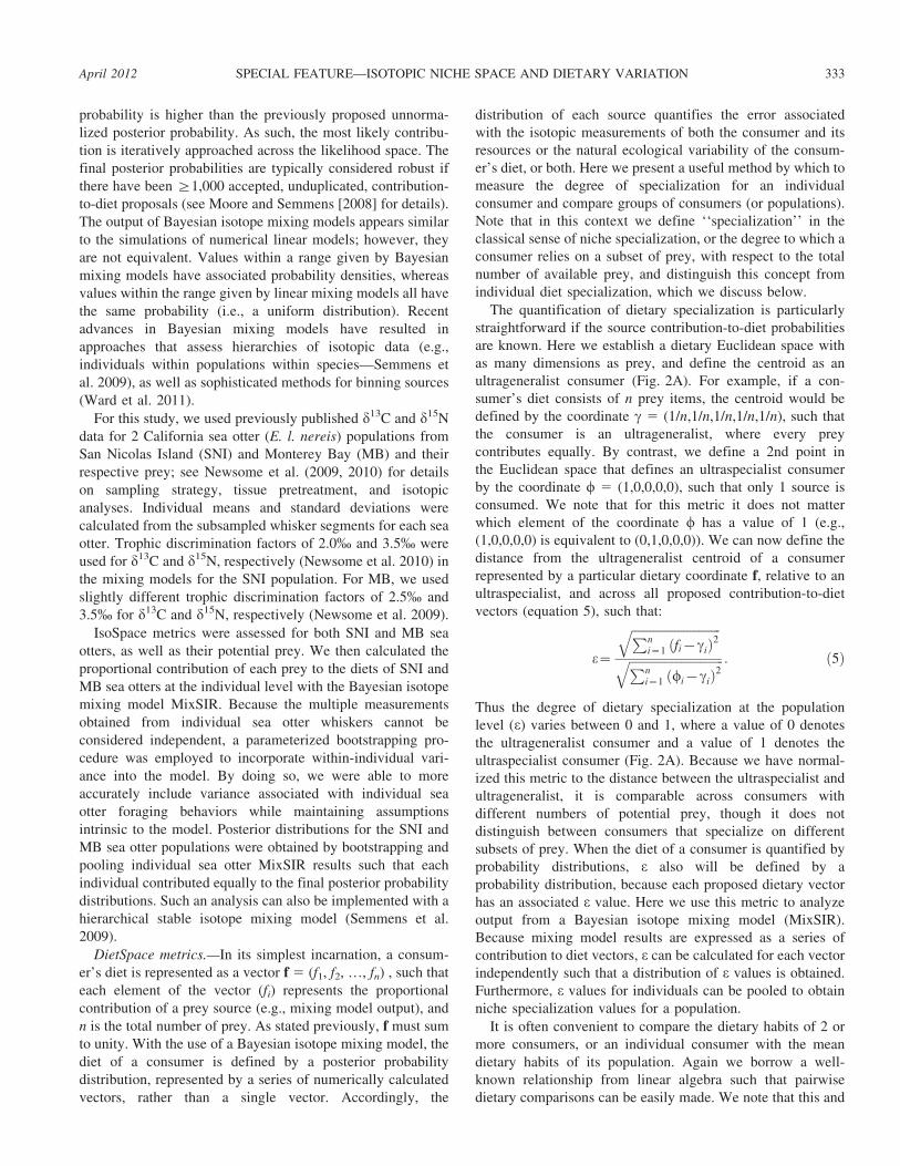
Stable isotope mixing models.—We used the Bayesian-based stable isotope mixing model MixSIR (version 1.0.4—Moore and Semmens 2008) to calculate posterior probabilitydensities of the proportional contributions of prey to SNI andMB sea otter population diets. We used uninformative priorsand only accepted results if there were #1,000 accepteddraws. Dietary contributions for SNI and MB populationswere calculated by bootstrapping and pooling MixSIR resultsfor individual sea otters in both populations; the densities aredisplayed in Fig. 4. Median (1st quartile, 3rd quartile)contribution estimates for the SNI sea otter population are:spiny lobsters + Cancer crabs 5 0.04 (0.01, 0.10); kelp crabs +sea urchins 5 0.26 (0.13, 0.41); abalone 5 0.20 (0.05, 0.40);Chlorostoma snails 5 0.26 (0.01, 0.66); and Megastraeasnails 5 0.03 (0.01, 0.09). Median (1st quartile, 3rd quartile)contribution estimates for the MB sea otter population are:purple sea urchins + mussels 5 0.02 (0.01, 0.05); kelp crabs 50.38 (0.09, 0.61); abalone 5 0.04 (0.01, 0.13); Cancer crabs 50.17 (0.06, .028); Chlorostoma snails 5 0.05 (0.02, 0.15); and

TABLE 1.—Mean carbon (d13C) and nitrogen (d15N) values, sample sizes (n), associated variance, [C]/[N] ratios, and population-level dietcomposition (6SD) based on observational data for sea otter prey groups from San Nicolas Island and Monterey Bay, California.

Prey type Species n d13C SD d15N SD [C]/[N]

San Nicolas Island

Sea urchins Strongylocentrotus franciscanus 18 214.4 0.6 10.7 0.7 7.0 (1.5)

Strongylocentrotus purpuratusNorthern kelp crabs Pugettia producta 5 214.5 0.8 11.3 0.9 4.2 (0.2)

Rock crabs Cancer productus/C. antennarius 8 215.1 1.2 14.7 0.3 3.9 (0.3)

Spiny lobsters Panulirus interruptus 5 215.7 0.7 15.3 0.3 3.7 (0.2)

Chlorostoma snails Chlorostoma funebralis/C. eiseni/C. regina 5 214.3 0.8 12.8 0.9 3.9 (0.1)Megastraea snails Megastraea undosa 5 219.1 0.5 11.2 0.3 3.8 (0.1)

Abalone Haliotis cracherodii/H. rufescens 22 215.5 0.9 9.5 0.9 3.6 (0.3)

Monterey Bay

Rock crabs Cancer productus/C. antennarius/C. magister 34 215.6 0.8 14.1 0.8 4.1 (0.2)

Purple sea urchins Strongylocentrotus purpuratus 16 217.0 1.1 9.4 0.4 4.7 (0.8)Clams Tresus nuttalli/Protothaca staminea/Saxidomus

nuttalli/Macoma nasuta

56 215.5 1.0 11.4 0.7 4.1 (0.5)

Northern kelp crabs Pugettia producta 27 213.3 1.1 11.6 0.8 4.8 (0.6)

California mussels Mytilus californianus 18 217.5 0.9 9.2 0.5 4.0 (0.4)Chlorostoma snails Chlorostoma funebralis 24 214.3 0.9 10.6 0.7 4.5 (0.4)

Chlorostoma pulligo/C. brunnea/C. montereyi

Abalone Haliotis cracherodii/H. rufescens 22 215.5 0.9 9.5 0.9 3.8 (0.3)


clams 5 0.04 (0.02, 0.11). Note that modeling results show afew cases where posterior probability distributions aremultimodal or highly variable, such that the median is notan optimal descriptive statistic.

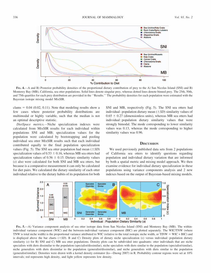
DietSpace metrics.—Niche specialization indexes werecalculated from MixSIR results for each individual withinpopulations SNI and MB; specialization values for thepopulation were calculated by bootstrapping and poolingindividual sea otter MixSIR results such that each individualcontributed equally to the final population specializationvalues (Fig. 5). The SNI sea otter population had mean (6SD)specialization values of 0.53 6 0.16, whereas MB sea otters hadspecialization values of 0.56 6 0.15. Dietary similarity values(s) also were calculated for both SNI and MB sea otters, butbecause is a comparative measurement it can only be calculatedfor diet pairs. We calculated the dietary similarity of each otterindividual relative to the dietary habits of its population for both

SNI and MB, respectively (Fig. 5). The SNI sea otters hadindividual : population dietary mean (6SD) similarity values of0.65 6 0.27 (dimensionless units), whereas MB sea otters hadindividual : population dietary similarity values that werestrongly bimodal. The mode corresponding to lower similarityvalues was 0.13, whereas the mode corresponding to highersimilarity values was 0.96.

DISCUSSION

We used previously published data sets from 2 populationsof California sea otters to identify questions regardingpopulation and individual dietary variation that are informedby both a spatial metric and mixing model approach. We thenexamine evidence for individual dietary specialization in thesepopulations using variance components analysis and 2 newindexes based on the output of Bayesian-based mixing models.

FIG. 5.—A) Variance component analysis of sea otter isotope data from San Nicolas Island (SNI) and Monterey Bay (MB). The within-individual variance component (WIC) and the between-individual variance component (BIC) are plotted separately. The WIC/TNW (whereTNW is total niche width) is the proportional variance attributed to WIC (relative to the total isotopic niche width, or TINW 5 WIC + BIC) andis displayed above the bar charts (6SD). B and C) Density plots of dietary niche specialization (e) versus individual : population dietarysimilarity (s) for B) SNI and C) MB sea otter populations. Density plots can be subdivided into quadrants: otter individuals that are nichespecialists with diets dissimilar to the population (specialist/dissimilar), niche specialists with diets similar to the population (specialist/similar),niche generalists with diets dissimilar to the population (generalist/dissimilar), and niche generalists with diets similar to the population(generalist/similar). Densities were drawn with a kernel density estimator (ks—Duong 2007) in R. Probability contour regions were set at 10%intervals; red represents high density, and light yellow represents low density.

FIG. 4.—A and B) Posterior probability densities of the proportional dietary contribution of prey to the A) San Nicolas Island (SNI) and B)Monterey Bay (MB), California, sea otter populations. Solid lines denote singular prey, whereas dotted lines denote binned prey. The 25th, 50th,and 75th quartiles for each prey distribution are provided in the ‘‘Results.’’ The probability densities for each population were estimated with theBayesian isotope mixing model MixSIR.


We also discuss challenges and caveats with the use of thesetools and offer new ways isotopic data may be utilized toidentify differences in population- and individual-level dietaryvariation.

IsoSpace metrics.—The isotopic patterns presented as d13Cversus d15N biplots among the sea otter populations in Fig. 3clearly suggest a difference in dietary variation at thepopulation level. The amount of variation among individualsat SNI (Fig. 3A) is lower than at MB (Fig. 2B), and thisdistinction is accurately captured in the significantly largerCHA estimate (t156 5 219.4, P , 0.001) for the MB versusSNI population. The degree of isotopic variation amongconsumers in a population is fundamentally driven by theamount of variation among prey sources available to eachpopulation. Thus, spatial metrics as applied solely to consumerisotopic data with no consideration of variation among putativeprey is problematic and can lead to flawed interpretations ofdietary variation, individual specialization, and food-webstructure (Hoeinghaus and Zeug 2008; Matthews and Mazum-der 2004). To account for isotopic variation in prey available toeach sea otter population, we calculated the CHA for the preyand present the percentage of this area occupied by each seaotter population (Fig. 3C). Despite removing a single preyspecies (Megastraea snails) at SNI that significantly reducedCHA estimates for prey at this locality (t190.9 5 20.9, P ,0.001), the sea otters occupied a significantly lower proportionof the prey space than at MB (t99.9 5 25.64, P , 0.001). Thissuggests that otters at SNI are using a smaller portion of theavailable niche space, and that interindividual dietary variationis larger at MB in comparison to SNI.

As with any data set, the existence of outliers can lead to anoverestimation of the CHA of prey or consumer, or both,isotopic space. Calculation of CHA with and without outliers,as done here with Megastraea snails at SNI, is one way ofassessing their impact. The DC metric is a 2nd useful methodfor assessing the degree of isotopic variation, but is lesssensitive to the effects of outliers than CHA because itincludes all individuals in a data set, not just those on theperiphery that define the convex hull. For example, the mean(6SD) DC of MB sea otters (1.1 6 0.5) was slightly, but notsignificantly (t96.6 5 1.87, P 5 0.06), larger than that of SNIsea otters (0.8 6 0.4). A 3rd measurement, the NND, isanother informative method to assess the relative distributionof prey and consumer data in isotopic biplots. The mean (6SD)NND among sea otters is similar (P . 0.3) at SNI (0.3 6 0.2)and MB (0.3 6 0.1), providing support that the significantdifference in CHA between the 2 populations is driven bypopulation-level dietary variation rather than the presence ofoutliers in the MB data set.

A discussion of outliers and the relative distribution of datain bivariate space highlights differences in the nature ofmixing spaces that can affect the utility of spatial metrics. Lowvariance in the mean NND and DC metrics is characteristic ofan even distribution of data in bivariate space. In contrast,when most prey are distributed along the periphery of themixing space, the existence of outliers can create a large

degree of variance in NND and DC metrics. For comparisonamong populations or communities, a comparison of NND andDC variance (i.e., standard deviation) provides an easy way todetermine whether differences in CHA result from outliers inbivariate space. The NND and DC metrics for the SNI and MBsea otters (Fig. 3) have similar standard deviations, suggestingthat the distribution of data points in d13C versus d15Nbivariate space is similar between the 2 populations. Thissupports the hypothesis that the significant difference in CHAbetween SNI and MB is indeed driven by a difference indietary variation at the population level, and not because theCHA of 1 population (MB) is inflated because of outliers. Thisconcept also has implications for the use of mixing models tointerpret isotopic data (see below).

Lastly, the difference in sample sizes among individuals in apopulation or species in a community is a factor to considerwhen interpreting spatial metrics. For example, we only havedata for 13 sea otters from SNI, but data for more than 30individuals from MB. In this particular scenario, the smalloverall sea otter population at SNI (n 5 30–40—Hatfield2005) mediates the discrepancy in sample size, because the 13individuals analyzed here represent a large portion (approx-imately 30–40%) of the total population in 2003 whenvibrissae were collected. Although larger, the approximately30 MB individuals represent a much smaller fraction(approximately 5%) of the sea otter population in MB. Insituations where population sizes are unknown, yet samplesizes are uneven among populations or species, a bootstrapmodeling approach can be used. Such an approach wouldrandomly select x number of individuals from the larger of the2 data sets, where x equals the total number of individualsanalyzed in the smaller data set, and calculate a spatial metric(e.g., CHA or NND) several thousand times to provide aconservative estimate of the mean and variance for a subset ofindividuals in the population for which there are more data.

Stable isotope mixing model.—When feasible, the use ofstable isotope mixing models to convert isotopic data inresource proportion estimates provides the most usefulecological information that can be directly compared totraditional types of data. Mixing models are ideal for scenarioswhen trying to parse dietary information among 3 sources (i.e.,prey) using 2 isotope systems, or between 2 sources using asingle isotope system. As mentioned above, most ecologicalscenarios are much more complex than these ideal situations,and our example of California sea otters is no exception.

Observational data from SNI and MB show that sea ottersconsume more than 30 species of invertebrate prey, withsubstantial overlap in the prey species available to eachpopulation. For our isotopic study, we chose to analyze the 7most important prey species for each population (Fig. 3),which based on observational data combine to represent.95% and approximately 90% of the prey consumed at SNIand MB, respectively (Table 2). In some situations, 2 preytypes had similar mean d13C and d15N values and we chose togroup them into a single source for the mixing models(Phillips et al. 2005). In some cases this strategy produced


combinations of prey with similar ecological functions (e.g.,Cancer crabs and spiny lobsters at SNI). Other combinations,however, did not include prey types with similar functions,such as purple sea urchins (macroalgae grazer–browser) andmussels (filter feeders) at MB. This overlap is likely related tothe large variation in d13C values of various types ofmacroalgae (e.g., brown versus red) previously reported fromCalifornia kelp forest ecosystems (Hamilton et al. 2011; Pageet al. 2008). In general, however, the isotopic patternsobserved among kelp forest invertebrates in California(Fig. 3) conform to expectations based on the isotopicgradients associated with primary producers (i.e., macroalgaeversus microalgae) and food-web structure (i.e., trophic level).

We used a Bayesian-based mixing model (MixSIR version1.0.4—Moore and Semmens 2008) to determine sourceproportions of the various prey types or groups in the diets ofthe 2 sea otter populations (Fig. 4). Again, the sea otter scenariopresented here is unique because the overall performance ofmixing models can be judged because we know a priori therelative contributions of prey types for these populations basedon observational data (Table 1; Tinker et al. 2008). At SNI,mixing model results (Fig. 4) identify the most important preyitems consumed by sea otters; however, the relative contribu-tions of prey in the population’s diet do not conform toobservational data. For example, the median contribution forthe sea urchin–kelp crab prey group was 26%, whereobservational data show that these 2 prey types combine tocontribute 82% of diet (Table 2). The mixing model alsosuggests that abalone (20%) and Chlorostoma snails (26%)were more important dietary components than shown byobservational data (1.8% and 3.3%, respectively). Other preytypes consumed by this population have relatively minormedian contributions, which is supported by the observationaldata (Table 2). This pattern, where only 2 or 3 prey typescombine to represent the large majority of resources consumedby this population, also is supported by spatial metrics.Estimates of CHA, NND, and DC for the sea otters at SNIare small relative to those for the prey types available to thepopulation (Fig. 3A). In addition, sea otters occupy a smallproportion of the available prey mixing space (Fig. 3C).

Like the observational data, mixing model results for the MBsea otter population shows a more diverse and even contributionof prey that at SNI (Table 2). Similar to SNI, however, themodel does a poor job of capturing the relative proportions ofprey. For example, the mixing model shows that kelp crabs arethe most important prey type (Fig. 4) and overestimates thisprey’s contribution to population diet with a median contributionof 39% versus 11% via observation. Furthermore, the modelshows that the median contribution of sea urchins and mussels to

the population’s diet is only 2%, but observational data showthat this prey is the 2nd most common prey consumed by MBsea otters, contributing approximately 14% to the populationdiet (Table 2). Lastly, Cancer crabs combine to contribute about25% to diet based on observation, but the model shows that theseprey have a median contribution of 17%.

The Bayesian framework is not a panacea. As withtraditional linear mixing models, if the number of sources istoo large relative to the number of isotope systems (e.g., d13C)that are used, the answers provided by the model will behighly uncertain, because many source combinations maycontribute to the observed mix. The opposite is also true—ifall potential prey items are not included and residual variationis not explicitly estimated, results will be biased. Like anystatistical model, if sources of uncertainty—individual orpopulation variation, or variation in source estimates—areignored or modeled inappropriately, estimates may be biased.Furthermore, if inaccurate trophic discrimination factors orvariance in trophic discrimination factors are applied,erroneous posterior probabilities will result (Bond andDiamond 2011). Finally, the nature of mixing spaces canhave a dramatic impact on the resultant distributions. Forexample, if a straight line can be drawn between the mixture(i.e., consumer) and 2 consecutive sources in the isotopicmixing space, results for those 2 potential sources will behighly variable, because many combinations of one, the other,or both sources could contribute to the consumer.

DietSpace metrics.—In the discussion of spatial metrics andmixing models above, we focus on aspects of population-leveldiet. The conventional calculation of a population’s dietarybreadth integrates prey selection across all individuals butignores inter- and intraindividual variation in diet. A growingnumber of studies, however, show that individual dietaryspecialization (or individuality) is pervasive in many taxa andcommunities (Bolnick et al. 2003). The growing recognitionof individuality in diet has important implications forpopulation biology, food-web dynamics, and stability (Kon-doh 2003), and may even contribute to interindividualvariation in fitness (Annett and Pierotti 1999; Darimont etal. 2007) that may result in phenotypic diversification andspeciation (Moodie et al. 2007; Svanback and Bolnick 2005).

Some recent studies (Lewis et al. 2006; Newsome et al.2009, 2010) have shown that an isotopic approach is a reliableand cost-effective alternative to observational or gut contentdata (Estes et al. 2003; Tinker et al. 2008; Werner and Sherry1987) that has been traditionally used to assess dietaryspecialization at the sex or individual level. Here we comparea previously published approach, variance component analysis(Newsome et al. 2009), with 2 novel indexes to assess

TABLE 2.—Diet composition for California sea otter populations at San Nicolas Island (SNI) and Monterey Bay (MB) based on observationand reported as the percentage of consumed organic biomass. Numbers in parentheses represent standard error of dietary contribution at thepopulation level based on observation of n number of individuals.

n Sea urchins Kelp crabs Cancer crabs Spiny lobsters Snails Mussels Clams Abalone

SNI 11 70.9 (5.0) 11.2 (1.6) 7.7 (3.1) 3.9 (2.2) 3.3 (0.6) 0.0 0.8 (0.6) 1.8 (1.2)

MB 28 14.4 (3.0) 11.0 (2.2) 25.0 (4.3) 0.0 9.3 (3.9) 10.3 (3.8) 12.9 (4.1) 6.4 (2.6)


individuality in the SNI and MB sea otter populations. The 2latter indexes, specialization index (e) and individual : popula-tion similarity (s), are based on the output of the Bayesian-based mixing model (Fig. 4). In contrast, the variancecomponents analysis only uses isotopic data from sea otters(not prey) to evaluate the within-individual components (WIC)and between-individual components (BIC) of diet.

The variance components results show there is nearly twiceas much isotopic variance in the MB sea otter data set than fromSNI (Fig. 5A), and that this pattern is driven by differences inthe BIC (SNI 5 0.77 versus MB 5 1.40). Traditionally, the totalniche width (TNW) of a population has been defined as thesum of the WIC and BIC of diet (Roughgarden 1972), andthe ratio of the WIC to the TNW (WIC/TNW) of a populationhas traditionally been used to evaluate individual specializa-tion (Bolnick et al. 2002). As WIC/TNW approaches 1, allindividuals utilize the full spectrum of resources used by thepopulation (i.e., all individuals are generalists), whereas a valueclose to 0 denotes that individuals are utilizing a smallproportion of resources consumed at the population level. Inother words, individual specialization increases as the WIC/TNW decreases. In a similar fashion, we can calculate a totalisotopic niche width (TINW) for each population by summingthe WIC and BIC in the isotopic data set (TINW 5 WIC +BIC). The mean (6SD) WIC/TINW for the MB population(0.33 6 0.03) was lower than that of the SNI population (0.40 60.08), suggesting a greater degree of individual specialization atMB versus SNI, which is also supported by observation(Table 2; Tinker et al. 2008).

As an alternative to the WIC/TINW index, we use ourspecialization metric (e) to assess the degree of nichespecialization for SNI and MB sea otter individuals. Thebenefit of this approach is that it does not require estimates ofwithin-individual dietary variation, even though we do includewithin-individual variability in our analysis of sea otter diet.When isotope data are used to calculate e, however, bothpredator and potential prey isotopic values are required tocalculate the proportional contribution of each prey to apredator’s diet. Because isotopic approaches are often of mostuse when quantifying species interactions that are difficult orimpossible to observe directly, we suggest that this approachhas merit. We observe that at both the population andindividual level, the MB sea otters have higher specializationvalues than the SNI sea otters, which is qualitatively similar tothe WIC/TINW metric (Fig. 5A).

An integration of the specialization metric with the measure-ment for individual : population dietary similarity (s) mayelucidate more information regarding sea otter diet (Fig. 5).Here we observe that most individuals at SNI have highsimilarity to the population mean (high s values), and rangefrom being niche specialists to generalists. A few individualsexhibit slightly different diets, represented by much weakerpeaks at lower values of s. By contrast, MB sea otters havesimilarity values that are strongly bimodal, a pattern associatedwith a high degree of individuality, with individuals falling into1 of a number of potential specialist types.

The analysis of SNI and MB sea otters with our proposedDietSpace metrics presents a straightforward means to assessniche specialization and dietary similarity with mixing modeloutput derived from isotopic measurements. Our resultsconfirm the expectation that SNI sea otters are more similarto the population as a whole, whereas MB sea otters are morevariable. Our results also confirm that the degree of nichespecialization at the individual level is generally high for theMB sea otters, whereas the greater range in similarity valuesindicates that there is greater population dietary diversity atMB. A result that is less obvious when analyzing only isotopicdata is that SNI sea otters span a range of niche specializationvalues and have low individuality (high s values), suggestingthat individuals are less likely to include prey that is lesspreferred at the population level.

Future developments and words of caution.—Stable isotopeanalysis is often attractive to ecologists because the results arenumerical data and naturally lend themselves to descriptivestatistics and quantitative manipulation. We foresee a strongfuture for quantitative tools that aid ecologists in interpretingisotopic data from the individual to community level. Futurework, however, should look back at potential weaknesses in anisotopic approach; in particular ecologists should examineassumptions that underpin isotopic mixing models. Martınezdel Rio et al. (2009b) demonstrated that inter- and intrataxonvariation in isotope trophic discrimination factors can varydepending upon a number of factors. These discriminationfactors are central in placing the consumer in the mixing spaceand affect some of the IsoSpace metrics and, to an unknowndegree, the isotopic mixing models. Bond and Diamond(2011) found that mixing model results are highly contingentupon discrimination factors, but this likely depends upon thenature of the IsoSpace.

The similarity among functionally distinct prey groups at MBhighlights an important caveat in using an isotopic approach tostudy variation in resource (or habitat) use. Isotopic data do nottypically provide dietary composition data at the species level.Instead, isotopic variation within or among ecosystems iscreated by biochemical processes, such as the formation of a3-carbon or 4-carbon sugar in the 1st step of photosynthesis orthe transamination–deamination of amino acids in the tricar-boxylic acid cycle that occurs during nutrient assimilation andamino acid synthesis. Biological processes that sort isotopes alsocan be driven by physicochemical variation in the environment(e.g., temperature), which governs the rate of biochemicalreactions by which organisms assimilate nutrients, grow, andreproduce. Stable isotope analysis will only be useful whenpotential sources (prey) have distinct isotope values (but seeYeakel et al. 2011) and an ideal approach would be to combinestable isotope analysis with traditional diet proxies (e.g., scatanalysis) that provide higher-resolution information on dietarydiversity.

Finally, we look to the future of DietSpace metrics andother ways to assess individuality with isotope data. Weanticipate that further quantitative descriptors relating dietarysimilarity or differences either among individuals or among


populations will be useful in a number of ecological subfields.One potential example is a metric of DietSpace that useshierarchical clustering to create a tree of dietary similarity.Such an approach could be used at the population level toexamine animals that compete for resources. At the individuallevel, a dietary tree of individuals could be compared togenetic data to determine if foraging behavior is culturallytransmitted from parents to offspring. As isotopic researchcontinues and techniques improve in accuracy and rigor weexpect that researcher creativity and ingenuity in exploringtheir data will expand as well. We welcome the furtherdevelopment of tools that seek to translate isotopic measure-ments into a language that can be understood by all ecologists.

ACKNOWLEDGMENTS

Thanks to the Monterey Bay National Marine Sanctuary Founda-tion and the United States Marine Mammal Commission for fundingthe collection and processing of sea otter prey samples. We thank A.Green, M. Kenner, K. Miles, and J. Bodkin for assistance in preycollection and E. Snyder, C. Mancuso, W. Wurzel, E. Heil, and R.Harley for laboratory assistance. We thank A. C. Jakle, E. J. Ward,and L. Feliciti for constructive reviews. We thank A. Green forobtaining the necessary California Fish and Game permit for marineinvertebrate collection and the United States Navy for permission toconduct research on San Nicolas Island. SDN was partially funded bythe National Science Foundation (ATM-0502491, DIOS-0848028),Carnegie Institution of Washington, and the W. M. Keck Foundation(072000). S. D. Newsome and J. D. Yeakel contributed equally to thisstudy.

LITERATURE CITED

ANNETT, C. A., AND R. PIEROTTI. 1999. Long-term reproductive outputin western gulls: consequences of alternate tactics in diet choice.Ecology 80:288–297.

BHATTACHARYYA, A. 1943. On a measure of divergence between twostatistical populations defined by their probability distributions.Bulletin of the Calcutta Mathematical Society 35:99–109.

BOLNICK, D. I., ET AL. 2003. The ecology of individuals: incidence andimplications of individual specialization. American Naturalist161:1–28.

BOLNICK, D. I., L. H. YANG, J. A. FORDYCE, J. M. DAVIS, AND R.SVANBACK. 2002. Measuring individual-level resource specializa-tion. Ecology 83:2936–2941.

BOND, A., AND A. DIAMOND. 2011. Recent Bayesian stable-isotopemixing models are highly sensitive to variation in discriminationfactors. Ecological Applications 21:1017–1023.

BOWEN, G. H., L. CHESSON, K. NIELSON, T. E. CERLING, AND J.EHLERINGER. 2005. Treatment methods for the determination of d2Hand d18O of hair keratin by continuous-flow isotope-ratio massspectrometry. Rapid Communications in Mass Spectrometry19:2371–2378.

CARLETON, S. A., L. KELLY, R. ANDERSON-SPRECHER, AND C. MARTINEZ

DEL RIO. 2008. Should we use one-, or multi-compartment modelsto describe 13C incorporation into animal tissues? Rapid Commu-nications in Mass Spectrometry 22:3008–3014.

CERLING, T. E., ET AL. 2007. Stable isotopic niche predicts fitness of preyin a wolf–deer system. Biological Journal of the Linnean Society90:125–137.

DARIMONT, C. T., P. C. PAQUET, T. E. REIMCHEN. 2007. Stable isotopeniche predicts fitness of prey in a wolf-deer system. BiologicalJournal of the Linnean Society 90:125–137.

DEAN, T. A., ET AL. 2002. Food limitation and the recovery of seaotters following the ‘Exxon Valdez’ oil spill. Marine EcologyProgress Series 241:255–270.

DUONG, T. 2007. KS: kernel density estimation and kerneldiscriminant analysis for multivariate data in R. Journal ofStatistical Software 21:1–16.

ELTON, C. S. 1927. Animal ecology. Sidgwick and Jackson, London,United Kingdom.

ESTES, J. A., M. L. RIEDMAN, M. M. STAEDLER, M. T. TINKER, AND B. E.LYON. 2003. Individual variation in prey selection by sea otters: patterns,causes and implications. Journal of Animal Ecology 72:144–155.

FARMER, A., B. S. CADE, AND J. TORRES-DOWDALL. 2008. Fundamentallimits to the accuracy of deuterium isotopes for identifying thespatial origin of migratory animals. Oecologia 158:183–192.

FLAHERTY, E. A., AND M. BEN-DAVID. 2010. Overlap and partitioningof the ecological and isotopic niches. Oikos 119:1409–1416.

FOOTE, M. 1990. Nearest-neighbor analysis of trilobite morphospace.Systematic Biology 39:371–382.

GAYE-SIESSEGGER, J., U. FOCKEN, H. ABEL, AND K. BECKER. 2003.Feeding level and diet quality influence trophic shift of C and Nisotopes in Nile tilapia (Oreochromis niloticus). Isotopes inEnvironmental and Health Studies 39:125–134.

GOULD, S. 1991. The disparity of the Burgess Shale arthropod faunaand the limits of cladistic analysis: why we must strive to quantifymorphospace. Paleobiology 17:411–423.

GRINNELL, J. 1917. The niche-relationships of the California thrasher.Auk 34:427–433.

HAMILTON, S. L., ET AL. 2011. Extensive geographic and ontogeneticvariation characterizes the trophic ecology of temperate reef fishon southern California rocky reefs. Marine Ecology Progress Series429:227–244.

HATFIELD, B. B. 2005. The translocation of sea otters to San NicolasIsland: an update. Pp. 473–475 in Proceedings of the 6th CaliforniaIslands Symposium (D. K. Garcelon and C. A. Schwemm, eds.).Institute for Wildlife Studies, Arcata, California National ParkService, Technical Publication CHIS-05-01.

HOEINGHAUS, D., AND S. ZEUG. 2008. Can stable isotope ratios providefor community-wide measures of trophic structure? Ecology89:2353–2357.

HUTCHINSON, G. E. 1957. Concluding remarks. Cold Spring HarborSymposia on Quantitative Biology 22:415–427.

HUTCHINSON, G. E. 1978. An introduction to population ecology. YaleUniversity Press, New Haven, Connecticut.

KOHN, A. J., AND A. C. RIGGS. 1982. Sample size dependence inmeasures of proportional similarity. Marine Ecology ProgressSeries 9:147–151.

KONDOH, M. 2003. Foraging adaptation and the relationship betweenfood-web complexity and stability. Science 299:1388–1391.

LAYMAN, C. A., ET AL. In press. Applying stable isotopes to examinefood-web structure: an overview of analytical tools. BiologicalReviews.

LAYMAN, C. A., D. A. ARRINGTON, C. G. MONTANA, AND D. M. POST.2007. Can stable isotope ratios provide for community-widemeasures of trophic structure? Ecology 88:42–48.

LEWIS, R., T. C. O’CONNELL, M. LEWIS, C. CAMPAGNA, AND A. R.HOELZEL. 2006. Sex-specific foraging strategies and resource parti-tioning in the southern elephant seal (Mirounga leonina). Proceed-ings of the Royal Society, B. Biological Sciences 273:2901–2907.


MARTINEZ DEL RIO, C., P. SABAT, R. ANDERSON-SPRECHER, AND S. P.GONZALEZ. 2009a. Dietary and isotopic specialization: the isotopicniche of three Cinclodes ovenbirds. Oecologia 161:149–159.

MARTINEZ DEL RIO, C., N. WOLF, S. A. CARLETON, AND L. Z. GANNES.2009b. Isotopic ecology ten years after a call for more laboratoryexperiments. Biological Reviews 84:91–111.

MATTHEWS, B., AND A. MAZUMDER. 2004. A critical evaluations ofintrapopulation variation of d13C and isotopic evidence ofindividual specialization. Oecologia 140:361–371.

MOODIE, G. E., P. F. MOODIE, AND T. E. REIMCHEN. 2007. Stableisotope niche differentiation in sticklebacks with symmetric andasymmetric pectoral fins. Biological Journal of the LinneanSociety 92:617–623.

MOORE, J. W., AND B. X. SEMMENS. 2008. Incorporating uncertaintyand prior information into stable isotope mixing models. EcologyLetters 11:470–480.

NEWSOME, S. D., ET AL. 2009. Using stable isotopes to investigateindividual diet specialization in California sea otters (Enhydralutris nereis). Ecology 90:961–974.

NEWSOME, S. D., M. T. CLEMENTZ, AND P. L. KOCH. 2010. Using stableisotope biogeochemistry to study marine mammal ecology. MarineMammal Science 26:509–572.

NEWSOME, S. D., C. MARTINEZ DEL RIO, S. BEARHOP, AND D. L. PHILLIPS.2007. A niche for isotopic ecology. Frontiers in Ecology and theEnvironment 5:429–436.

OFTEDAL, O. T., K. RALLS, M. T. TINKER, AND A. GREEN. 2007.Nutritional constraints on the southern sea otter in the MontereyBay National Marine Sanctuary. Monterey Bay National MarineSanctuary and Marine Mammal Commission, Washington, D.C.,Technical Report.

PAGE, H. M., D. C. REED, M. A. BRZEZINSKI, J. M. MELACK, AND J. E.DUGAN. 2008. Assessing the importance of land and marine sourcesof organic matter to kelp forest food webs. Marine EcologyProgress Series 360:47–62.

PARNELL, A. C., R. INGER, S. BEARHOP, AND A. L. JACKSON. 2010.Source partitioning using stable isotopes: coping with too muchvariation. PLoS ONE 5:e9672.

PHILLIPS, D. L., AND J. W. GREGG. 2003. Source partitioning usingstable isotopes: coping with too many sources. Oecologia 136:261–269.

PHILLIPS, D. L., AND P. L. KOCH. 2002. Incorporating concentrationdependence in stable isotope mixing models. Oecologia 130:114–125.

PHILLIPS, D. L., S. D. NEWSOME, AND J. W. GREGG. 2005. Combiningsources in stable isotope mixing models: alternative methods.Oecologia 144:520–527.

POST, D. 2002. Using stable isotopes to estimate trophic position:models, methods, and assumptions. Ecology 83:703–718.

RICCA, M. A., A. K. MILES, R. G. ANTHONY, X. DENG, AND S. S. O.HUNG. 2007. Effect of lipid extraction on analyses of stable carbonand stable nitrogen isotopes in coastal organisms of the Aleutianarchipelago. Canadian Journal of Zoology 85:40–48.

ROUGHGARDEN, J. 1972. Evolution of niche width. American Naturalist106:683–718.

SEMMENS, B. X., E. J. WARD, J. W. MOORE, AND C. T. DARIMONT. 2009.Quantifying inter- and intra-population niche variability usinghierarchical Bayesian stable isotope mixing models. PloS ONE4:e6187.

SMITH, E. P., K. W. PONTASCH, AND J. C. CAIRNS. 1990. Communitysimilarity and the analysis of multispecies environmental data: aunified statistical approach. Water Research 24:507–514.

SVANBACK, R., AND D. L. BOLNICK. 2005. Intraspecific competitionaffects the strength of individual specialization: an optimal diettheory method. Evolutionary Ecology Research 7:993–1012.

TINKER, M. T., G. BENTALL, AND J. A. ESTES. 2008. Food limitationleads to behavioral diversification and dietary specialization in seaotters. Proceedings of the National Academy of Sciences 105:560–565.

TURNER, F. T., M. L. COLLYER, AND T. J. KRABBENHOFT. 2010. Ageneral hypothesis-testing framework for stable isotope ratios inecological studies. Ecology 91:2227–2233.

VANDER ZANDEN, M. J., AND J. B. RASMUSSEN. 2001. Variation in d15Nand d13C trophic fractionation: implications for aquatic food webstudies. Limnology and Oceanography 46:2061–2066.

WARD, E. J., B. X. SEMMENS, D. L. PHILLIPS, J. W. MOORE, AND N.BOUWES. 2011. A quantitative approach to combine sources instable isotope mixing models. Ecosphere 2:art19.

WATTERS, G. T. 1991. Utilization of a simple morphospace bypolyplacophorans and its evolutionary implications. Malacologia33:221–240.

WERNER, T. K., AND T. W. SHERRY. 1987. Behavioral feedingspecialization in Pinaroloxias inornata, the ‘‘Darwin’s finch’’ ofCocos Island, Costa Rica. Proceedings of the National Academy ofSciences 84:5506–5510.

WINEMILLER, K. 1991. Ecomorphological diversification in lowlandfreshwater fish assemblages from five biotic regions. EcologicalMonographs 61:343–365.

WUNDER, M. B., AND D. R. NORRIS. 2008. Improved estimates ofcertainty in stable-isotope–based methods for tracking migratoryanimals. Ecological Applications 18:549–559.

YEAKEL, J. D., ET AL. 2011. Merging resource availability with isotopemixing models: the role of neutral interaction assumptions. PLoSONE 6:e22015.

Special Feature Editor was Samantha M. Wisely.


tools for quantifying isotopic niche space and dietary variation at …. mammal. 2012...

Documents