tolerance intervals for discrete …tcai/paper/tolerance...statistica sinica 19 (2009), 905-923...

Statistica Sinica 19 (2009), 905-923

TOLERANCE INTERVALS FOR DISCRETE DISTRIBUTIONS

IN EXPONENTIAL FAMILIES

Tianwen Tony Cai and Hsiuying Wang

University of Pennsylvania and National Chiao Tung University

Abstract: Tolerance intervals are widely used in industrial applications. So far

attention has been mainly focused on the construction of tolerance intervals for

continuous distributions. In this paper we introduce a unified analytical approach

to the construction of tolerance intervals for discrete distributions in exponential

families with quadratic variance functions. These tolerance intervals are shown to

have desirable probability matching properties and outperform existing tolerance

intervals in the literature.

Key words and phrases: Coverage probability, Edgeworth expansion, exponential

family, probability matching, tolerance interval.

1. Introduction

Statistical tolerance intervals are important in many industrial applicationsranging from engineering to the pharmaceutical industry. See, for example, Hahnand Chandra (1981) and Hahn and Meeker (1991). The goal of a toleranceinterval is to contain at least a specified proportion of the population, β, with aspecified degree of confidence, 1−α. More specifically, let X be a random variablewith cumulative distribution function F . An interval (L(X), U(X)) is said to be aβ-content, (1−α)-confidence tolerance interval for F (called a (β, 1−α) toleranceinterval for short) if

P{[F (U(X)) − F (L(X))] ≥ β} = 1 − α. (1.1)

One-sided tolerance bounds can be defined analogously. A bound L(X) is said tobe a (β, 1−α) lower tolerance bound if P{1−F (L(X)) ≥ β} = 1−α and a boundU(X) is said to be a (β, 1−α) upper tolerance bound if P{F (U(X)) ≥ β} = 1−α.

Ever since the pioneering work of Wilks (1941, 1942), construction of tol-erance intervals for continuous distributions has been extensively studied. See,for example, Wald and Wolfowitz (1946), Easterling and Weeks (1970), Kocher-lakota and Balakrishnan (1986), Vangel (1992), Mukerjee and Reid (2001), andKrishnamoorthy and Mathew (2004). Compared with the continuous distribu-tions, literature on tolerance intervals for discrete distributions is sparse. This is

906 TIANWEN TONY CAI AND HSIUYING WANG

mainly due to the difficulty in deriving explicit expression for the tolerance in-tervals in the discrete case. Zacks (1970) proposed a criterion to select tolerancelimits for monotone likelihood ratio families of discrete distributions. The mostwidely used tolerance intervals to date for Poisson and Binomial distributionswere proposed by Hahn and Chandra (1981). The intervals are constructed by atwo-step procedure. See Hahn and Meeker (1991) for a survey of these intervals.

Although tolerance intervals are useful and important, their properties, suchas their coverage probability, have not been studied as much as those of confidenceintervals. As we shall see in Section 2, the tolerance intervals given in Hahnand Chandra (1981) tend to be very conservative in terms of their coverageprobability. Techniques for the construction of tolerance intervals in the literatureoften vary from distribution to distribution.

In this paper, we introduce a unified analytical approach using the Edgeworthexpansions for the construction of tolerance intervals for the discrete distributionsin exponential families with quadratic variance functions. We show that thesetolerance intervals enjoy desirable probability matching properties and outper-form existing tolerance intervals in the literature. The most satisfactory aspectsof our results are the constancy of the phenomena, and uniformity in the finalresolutions of these problems. Edgeworth expansions have also been used verysuccessfully for the construction of confidence intervals in discrete distributions.See Hall (1982), Brown, Cai and DasGupta (2002, 2003), and Cai (2005). Con-struction of tolerance interval is closely related to the construction of confidenceinterval for quantiles. A one-sided tolerance bound is equivalent to a one-sidedconfidence bound on a quantile of the distribution. See Hahn and Meeker (1991).Therefore, the proposed method can be also employed for the quantile estimationproblem.

The paper is organized as follows. We begin in Section 2 by briefly review-ing the existing tolerance intervals for Binomial and Poisson distributions andshowing that they have serious deficiencies in terms of coverage probability. Theserious deficiency of these intervals calls for better alternatives. After Section 3.1,in which basic notations and definitions of natural exponential family are summa-rized, the first-order and second-order probability matching tolerance intervalsare introduced. As in the case of confidence intervals, the coverage probabilityof the tolerance intervals for the lattice distributions such as Binomial and Pois-son distributions contains two components: oscillation and systematic bias. Theoscillation in the coverage probability, which is due to the lattice structure ofthe distributions, is unavoidable for any non-randomized procedures. The sys-tematic bias, which is large for many existing tolerance intervals, can be nearlyeliminated. We show that our new tolerance intervals have better coverage prop-erties in the sense that they have nearly vanishing systematic bias in all thedistributions under consideration.

TOLERANCE INTERVALS FOR DISCRETE DISTRIBUTIONS 907

In Section 4, two-sided tolerance intervals are constructed by using one-sided upper and lower probability matching tolerance bounds. In addition to thecoverage properties, parsimony in expected length of the two-sided intervals isalso discussed. Section Appendix is an appendix containing detailed technicalderivations of the tolerance intervals. The derivations are based on the two-termEdgeworth and Cornish-Fisher expansions.

2. Tolerance Intervals: Existing Methods

As mentioned in the introduction, we construct tolerance intervals for dis-crete distributions in the exponential families. In this section we review the ex-isting tolerance intervals for two important discrete distributions, the Binomialand Poisson distributions. These tolerance intervals will be used for comparisonwith the new intervals constructed in the present paper.

The most widely used method for constructing tolerance intervals for theBinomial and Poisson distributions was proposed by Hahn and Chandra (1981).Suppose x is the observed value of a random variable X having a Binomialdistribution B(n, θ) or a Poisson distribution Poi(nθ), and that one wishes toconstruct a tolerance interval based on x. The method introduced by Hahn andChandra (1981) for constructing a (β, 1−α) tolerance interval (L(x), U(x)) hastwo steps.

(i) Construct a two-sided (1 − α)-level confidence interval (l, u) for θ, where l

and u depends on x.(ii) Find the minimum number U(x) and the maximum number L(x) such that

p(X ≤ U(x)|θ = µ) ≥ 1 + β

2and p(X > L(x)|θ = l) ≥ 1 + β

2.

Similarly, a lower (β, 1 − α) tolerance bound L(x) can be constructed byfinding a lower (1 − α) confidence bound of θ, say l, and then deriving themaximum value L(x) such that pl(X > L(x)) ≥ β.

For this two-step procedure, it is clear that the choice of the confidenceinterval used in Step 1 is important to the performance of the resulting toleranceinterval. For any 0 < γ < 1, let zγ = Φ−1(1 − γ) be the 1 − γ quantile of astandard normal distribution. Hahn and Meeker (1991) suggested (1 − α) levelconfidence intervals for the Binomial case,

(l, u)= θ̂ ± zα/2

( θ̂(1 − θ̂)n

)1/2, (2.1)

(l, u)=((

1+(n−x+1)F(α/2;2n−2x+2,2x)

x

)−1,(1+

n−x

(x+1)F(α/2;2x+2,2n−2x)

)−1)

,(2.2)


where F(a;r1,r2) denotes the 1 − a quantile of the F distribution with r1 and r2

degrees of freedom. For the Poisson distribution, the suggested (1−α) confidenceintervals in Hahn and Meeker (1991) are

(l, u) = θ̂ ± zα/2

( θ̂

n

)1/2, (2.3)

(l, u) =

(0.5

χ2(α/2;2x)

n, 0.5

χ2(1−α/2;2x+2)

n

), (2.4)

where χ2(a;r1) is a quantile of the chi-square distribution with r1 degrees of free-

dom. The θ̂ in (2.1) and (2.3) denotes the sample mean. The confidence boundsfor one-sided tolerance intervals in both Binomial and Poisson distributions aregiven analogously.

Figure 1 presents the coverage probabilities of both the two-sided and one-sided tolerance intervals for the Binomial and Poisson distributions. It can easilybe seen from the plots that these tolerance intervals are too conservative withhigher or lower coverage probability than the nominal level for both distributions.

As in the case of confidence intervals, the coverage probability of the tol-erance intervals contains two components: oscillation and systematic bias. Theoscillation in the coverage probability, due to the lattice structure of the Bino-mial and Poisson distributions, is unavoidable for any non-randomized proce-dures. However, the systematic biases for the existing tolerance intervals aresignificantly larger than we expected. This is partly due to the poor behavior ofthe confidence intervals used in the construction of the tolerance intervals. Notethat (2.1) and (2.2) are the Wald and Clopper-Pearson intervals for the binomialproportion. It is known that these confidence intervals have poor performances.See, for example, Agresti and Coull (1998) and Brown et al. (2002). It is thuspossible to improve the performance of the tolerance intervals by using betterconfidence intervals, like those presented in Brown et al. (2002) for the binomialdistribution.

However, we do not take this approach here. The goal of this paper is toprovide a unified analytical approach to the construction of desirable toleranceintervals for exponential families with certain optimality properties. The resultsshow that the Edgeworth expansion approach is a powerful tool for solving thisproblem.

In Section 3 we introduce new tolerance intervals using the Edgeworth ex-pansion. These intervals have better coverage properties in the sense that theyhave nearly vanishing systematic bias. Figure 3 presents the coverage probabil-ities of the proposed two-sided tolerance intervals for the Binomial and Poisson


Figure 1. Coverage probabilities of the 90%-content, 95% level two-sided(top two rows) and one-sided (bottom two rows) tolerance intervals for theBinomial and Poisson distributions with n = 50, where p is the probabilityof success for the binomial distribution.


distributions. Compared with Figure 1, the tolerance intervals certainly havemuch better performance than the existing intervals in the sense that the actualcoverage probability is much closer to the nominal level. The detailed derivationof our tolerance intervals is given in the next section.

3. Probability-Matching Tolerance Intervals

In this section we construct one-sided probability-matching tolerance inter-vals in the natural discrete exponential family (NEF) with quadratic variancefunctions (QVF) by using the Edgeworth expansion. After Section 3.1 in whichbasic notations and definitions of natural exponential family are given, we intro-duce the first-oder and second-order probability matching tolerance intervals inSection 3.2.

3.1. Natural exponential family

The NEF-QVF family contains three important discrete distributions: Bino-mial, Negative Binomial, and Poisson (see, e.g., Morris (1982) and Brown (1986).

We first state some basic facts about the NEF-QVF families. The distribu-tions in a natural exponential family have the form

f(x|ξ) = eξx−ψ(ξ)h(x),

where ξ is called the natural parameter. The mean µ, variance σ2 and cumulantgenerating function φξ are, respectively,

µ = ψ′(ξ), σ2 = ψ′′(ξ), and φξ(t) = ψ(t + ξ) − ψ(ξ).

The cumulants are given as Kr = ψ(r)(ξ). Let β3 and β4 denote the skewness andkurtosis. In the subclass with a quadratic variance function (QVF), the varianceψ′′(ξ) depends on ξ only through the mean µ and, indeed,

σ2 ≡ V (µ) = d0 + d1µ + d2µ2 (3.1)

for suitable constants d0, d1, and d2. We denote the discriminant by

∆ = d21 − 4d0d2. (3.2)

The notation ∆ is used in the statements of theorems for both the discrete andthe continuous cases, although for all the discrete cases ∆ happens to be equalto 1. Note that dµ/dξ = ψ′′(ξ) = σ2, so

K3 =ψ(3)(ξ)=dV

dµ· dµ

dξ=(d1+2d2µ)σ2 and K4 =ψ(4)(ξ)=

dK3

dµ· dµ

dξ=∆σ2+6d2σ

4.


Hence,

β3 =K3

σ3= (d1 + 2d2µ)σ−1 and β4 =

K4

σ4= ∆σ−2 + 6d2. (3.3)

Here are the important facts about the Binomial, Negative Binomial, andPoisson distributions.

• Binomial, B(1, p): ξ = log(p/q), ψ(ξ) = log(1+eξ), and h(x) = 1. Also µ = p,V (µ) = pq = µ − µ2. Thus d0 = 0, d1 = 1, d2 = −1,

β3 =1 − 2µ

(µ(1 − µ))1/2, and β4 =

1 − 6µ + 6µ2

µ(1 − µ).

• Negative Binomial, NB(1, p), the number of successes before the first failure:ξ = log p, ψ(ξ) = − log(1 − eξ), and h(x) = 1, where p is the probability ofsuccess. Here µ = p/q, and V (µ) = p/q2 = µ + µ2, so d0 = 0, d1 = 1, d2 = 1,

β3 =1 + 2µ

(µ(1 + µ))1/2, and β4 =

1 + 6µ + 6µ2

µ(1 + µ).

• Poisson, Poi(λ): ξ = log λ, ψ(ξ) = eξ, and h(x) = 1/x!. Then µ = λ, V (µ) =µ, and here d0 = 0, d1 = 1, d2 = 0,

β3 =1

µ1/2, and β4 =

1µ

.

3.2. One-sided tolerance interval

We now introduce the first-order and second-order probability matching one-sided tolerance intervals. Let X =

∑ni=1 Xi, where Xi are iid observations from

one of the three distributions discussed in Section 3.1. We denote the distributionof X by Fn,µ and focus our discussion on the lower tolerance intervals. The uppertolerance intervals can be constructed analogously. Two-sided tolerance intervalswill be discussed in Section 4.

Similar to confidence intervals, the coverage probability of a lower (β, 1−α)tolerance interval admits a two-term Edgeworth expansion of the general form

P (1 − Fn,µ(L(X)) ≥ β) = 1 − α + S1 · n−1/2 + Osc1 · n−1/2 + S2 · n−1

+Osc2 · n−1 + O(n−3/2), (3.4)

where the first O(n−1/2) term, S1n−1/2, and the first O(n−1) term, S2n

−1, are thefirst and second order smooth terms, respectively, and Osc1 ·n−1/2 and Osc2 ·n−1

are the oscillatory terms. (The oscillatory terms vanish in the case of continuous


distributions.) The smooth terms capture the systematic bias in the coverageprobability. See Bhattacharya and Rao (1976) and Hall (1982) for details onEdgeworth expansions.

We call a tolerance interval first-order probability matching if the first or-der smooth term S1n

−1/2 vanishes, and call the interval second-order probabilitymatching if both S1n

−1/2 and S2n−1 vanish. Note that the oscillatory terms are

unavoidable for any nonrandomized procedures in the case of lattice distribu-tions. See Ghosh (1994) and Ghosh (2001) for general discussions on probabilitymatching confidence sets.

Motivated by the discussion given at the end of this section, we consider anapproximate β-content, (1 − α)-confidence lower tolerance bound of the form

L(X) = X + a − b

√n(d0 +

d1X

n+

d2X2

n2) + c, (3.5)

where d0, d1 and d2 are the constants in (3.1), and a, b, and c are constantsdepending on α and β such that

L(X) < L(Y ) if X < Y. (3.6)

Remark. The quantity a in (3.5) “re-centers” the tolerance interval and, we seelater, a is important to the performance of the tolerance interval. The quantityc in (3.5) plays the role of a “boundary correction”. The parameter c is to beadjusted such that the coefficients S1 and S2 of the smooth terms n−1/2 andn−1 in (3.4) can be zero. The effect of c can be significant when µ is near theboundaries.

We use the Edgeworth expansion to choose the constants a, b, and c sothat the resulting tolerance intervals are first-order and second-order proba-bility matching. The first step in the derivation is to invert the constraint1 − F (L(X)) ≥ β to a constraint on X of the form X ≤ u(µ, β). Then thecoverage probability of the tolerance interval can be expanded using the Edge-worth expansion. The optimal choice of the values a, b, and c can then be solvedby setting the smooth terms in the expansion to zero. The algebra involved hereis more tedious than for deriving the probability matching confidence interval.The detailed proof is given in the Appendix.

Theorem 1. The tolerance interval given in (3.5) is first-order probability match-ing for the three discrete distributions in the NEF-QVF if

a =16[(z2

1−β − 1)(1 + 2d2µ̂) + (1 + 3zαz1−β + 2z2α)(d1 + 2d2µ̂)], (3.7)

b = zα + z1−β , (3.8)


and c = 0, where µ̂ = X/n and σ̂ =√

d0 + d1µ̂ + d2µ̂2. The tolerance interval(3.5) is second-order probability matching with a and b given as in (3.7) and (3.8),and c given by

c =1

36(zα + z1−β){(−1 + 18d0d2 + 2(−8 + 9d1)d2µ̂ + 2d2

2µ̂2)z3

1−β

+24d2(d0 + µ̂(d1 + d2µ̂))z21−βzα + z1−β[1 + 2d2µ̂(20 + 5d2µ̂ + 24d2µ̂z2

α)

+3d21(2 + z2

α) + 18d0d2(−3 + 2z2α) + 6d1d2µ̂(−5 + 8z2

α)] + zα[d21(7 + 2z2

α)

+2d1d2µ̂(5 + 13z2α) + 2d2(9d0(−1 + z2

α) + d2µ̂2(5 + 13z2

α))]}

. (3.9)

Remark. We have focused above on the construction of lower tolerance intervals.The first order and second order β-content, (1 − α)-confidence upper toleranceintervals can be constructed analogously as

X + a + b

√n(d0 +

d1X

n+

d2X2

n2), (3.10)

X + a + b

√n(d0 +

d1X

n+

d2X2

n2) + c, (3.11)

respectively, with the same a, b, and c as the lower tolerance intervals.For all three distributions, b = zα + z1−β . It is useful to give the expressions

of the constants a and c individually for each of the three distributions.

1. Binomial: a =16(1 − 2µ̂)(zα + z1−β)(2zα + z1−β), and

c = − 118

(13z2α + 11zαz1−β + z2

1−β + 5)(µ̂− µ̂2) +136

(2z2α + zαz1−β − z2

1−β + 7).

2. Poisson: a =16(zα + z1−β)(2zα + z1−β) and c =

136

(7− z21−β + zαz1−β + 2z2

α).

3. Negative Binomial: a =16(1 + 2µ̂)(zα + z1−β)(2zα + z1−β) and c =

118

(13z2α +

11zαz1−β + z21−β + 5)(µ̂ + µ̂2) +

136

(2z2α + zαz1−β − z2

1−β + 7).

We consider the discrete NEF-QVF family because the most important dis-crete distributions are there. Our results can be generalized to the discrete NEFfamily with variance functions of the form V (µ) = d0 +d1µ+d2µ

2 +d3µ3 +d4µ

4,because there exists a general solution for V (µ) = 0.

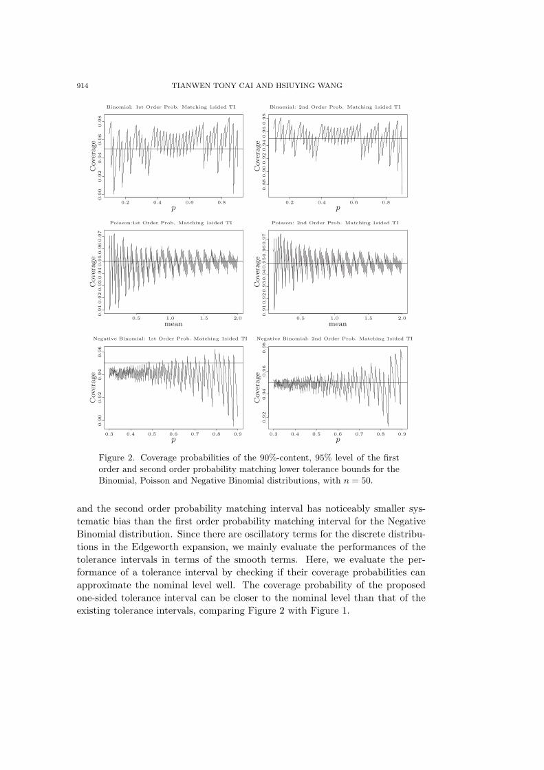
Figure 2 plots the coverage probabilities of the first-order and second-orderprobability matching (0.9, 0.95) lower tolerance intervals for n = 50. It is clearfrom Figure 2 that for the three discrete distributions, the first and second orderprobability matching tolerance intervals have nearly vanishing systematic bias,


Figure 2. Coverage probabilities of the 90%-content, 95% level of the firstorder and second order probability matching lower tolerance bounds for theBinomial, Poisson and Negative Binomial distributions, with n = 50.

and the second order probability matching interval has noticeably smaller sys-tematic bias than the first order probability matching interval for the NegativeBinomial distribution. Since there are oscillatory terms for the discrete distribu-tions in the Edgeworth expansion, we mainly evaluate the performances of thetolerance intervals in terms of the smooth terms. Here, we evaluate the per-formance of a tolerance interval by checking if their coverage probabilities canapproximate the nominal level well. The coverage probability of the proposedone-sided tolerance interval can be closer to the nominal level than that of theexisting tolerance intervals, comparing Figure 2 with Figure 1.


The motivation for considering the form (3.5) is briefly described as follows.Let X1, . . . , Xn be a sample from a normal distribution N(µ, σ2). Wald andWolfowitz (1946) introduced the β-content, (1−α)-confidence tolerance interval

[X̄ −√

n − 1χ2

n−1,α

tS, X̄ +

√n − 1χ2

n−1,α

tS], (3.12)

where X̄ and S are the sample mean and sample standard deviation, respectively,χ2

n−1,α is the α−quantile of the chi-squared distribution with n − 1 degrees offreedom, and t is the solution of the equation∫ 1√

n+t

1√n−t

1√2π

e−x2/2dx = β.

To make a better analogy between the NEF-QVF families and normal cases,we first attempt to rewrite the tolerance interval in (3.12) in terms of X =∑n

i=1 Xi under N(nµ, nσ2). Note that (3.12) implies

1 − α ≈ P (Φµ,σ(X̄ +

√n − 1χ2

n−1,α

tS) − Φµ,σ(X̄ −√

n − 1χ2

n−1,α

tS) ≥ β),

where Φµ,σ denotes the cdf of the N(µ, σ2) distribution. Since

Φµ,σ(X̄ ±√

n − 1χ2

n−1,α

tS) = Φnµ,√

nσ(nµ +√

n(X̄ − µ) ±√

n − 1χ2

n−1,α

t√

nS), (3.13)

and replacing µ by the lower or upper limits of a β-confidence confidence interval(X̄ − z(1−β)/2S/

√n, X̄ + z(1−β)/2S/

√n) for µ, we have the tolerance interval

[X−(

√n − 1χ2

n−1,α

t+(1− 1√n

)z(1−β)/2)√

ns, X+(

√n − 1χ2

n−1,α

t+(1− 1√n

)z(1−β)/2)√

ns]

under the N(nµ, nσ2) distribution.For the NEF-QVF families, by the Central Limit Theorem, and adopting

the method in the normal case by identifying d0 + d1X/n + d2X2/(n2) as s2,

an approximate β-content, (1 − α)-confidence tolerance lower bound and upperbound are X − A and X + A, respectively, where A = (

√n − 1/χ2

n−1,αt + (1 −1/√

n)z(1−β)/2)√

n(d0 + d1X/n + d2X2/n2). More generally, we consider toler-ance bounds of the form

L(X) = X + a − b

√n(d0 +

d1X

n+

d2X2

n2) + c

U(X) = X + a + b

√n(d0 +

d1X

n+

d2X2

n2) + c

with suitably chosen constants a, b, and c.


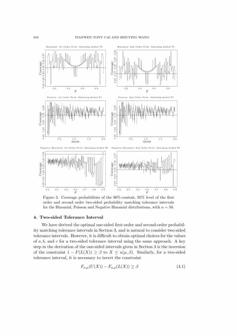
Figure 3. Coverage probabilities of the 90%-content, 95% level of the firstorder and second order two-sided probability matching tolerance intervalsfor the Binomial, Poisson and Negative Binomial distributions, with n = 50.

4. Two-sided Tolerance Interval

We have derived the optimal one-sided first-order and second-order probabil-ity matching tolerance intervals in Section 3, and is natural to consider two-sidedtolerance intervals. However, it is difficult to obtain optimal choices for the valuesof a, b, and c for a two-sided tolerance interval using the same approach. A keystep in the derivation of the one-sided intervals given in Section 3 is the inversionof the constraint 1 − F (L(X)) ≥ β to X ≤ u(µ, β). Similarly, for a two-sidedtolerance interval, it is necessary to invert the constraint

Fn,µ(U(X)) − Fn,µ(L(X)) ≥ β (4.1)


Figure 4. Expected lengths of the 90%-content, 95% level of the two-sidedtolerance interval based on (2)(solid, binomial) and (3)(dotted, binomial),the tolerance interval based on (4)(solid, Poisson) and (5)(dotted, Poisson),the first order probability matching two-sided tolerance interval (dashed) andthe second order probability matching two-sided tolerance interval (long-dashed) for Binomial (left panel) and Poisson (right panel) distributions,with n = 50. For the Poisson distribution, the dashed and long-dashed linesalmost overlap.

in terms of X. This is theoretically difficult.We thus take the alternative approach of using one-sided upper and lower

tolerance bounds. Let U(1+β)/2(X) and L(1+β)/2(X) be the upper and lowerprobability matching ((1+β)/2, 1−α) tolerance bounds, respectively. We proposeto use the interval

(L(1+β)/2(X), U(1+β)/2(X)) (4.2)

as a β-content, (1 − α)-confidence two-sided tolerance interval.Figure 3 plots the coverage probabilities of two-sided (0.9, 0.95) tolerance

intervals built from the first-order and second-order probability matching tol-erance bounds. The coverage probabilities for the two-sided tolerance intervalsare calculated exactly for the three discrete distributions. By comparing Figure3 with Figure 1, it is clear that the performance of these two-sided intervals isbetter than that of existing two-sided tolerance intervals in the case of Binomialand Poisson distributions. The coverage probability of the proposed two-sidedtolerance intervals oscillates in the center from 0.95 to 0.96 with a systematic biasless than 0.01. In contrast, the coverage probability of the two-sided toleranceintervals in Figure 1 oscillates in the center from 0.975 to 0.99 with a systematicbias greater than 0.025.

In addition to coverage probability, parsimony in length is also an importantissue. Figure 4 compares the expected length of the two new tolerance intervalswith that of the two intervals discussed in Section 2. It is clear that the expected


length of the proposed tolerance intervals is less than that of the existing toler-ance intervals. Thus, based on both coverage probability and expected length,the tolerance intervals derived from our analytical approach outperform existingtolerance intervals.

Acknowledgement

The research of Tony Cai was supported in part by NSF Grant DMS-0604954.

Appendix. Proof of Theorem 1

We begin by introducing notation and a technical lemma. All three discretedistributions under consideration are lattice distributions with the maximal spanof one. Lemma 1 below gives the Edgeworth expansion and Cornish-Fisher ex-pansion for these distributions. The first part is from Brown et al. (2003). Fordetails on the Edgeworth expansion and Cornish-Fisher expansion, see Esseen(1945), Petrov (1975), Bhattacharya and Rao (1976), and Hall (1982).

Let X1, . . . , Xn be iid observations from a discrete distribution in the NEF-QVF family. Denote the mean of X1 by µ and the standard deviation by σ. Letβ3 = K3/σ3 and β4 = K4/σ4 be the skewness and kurtosis of X1, respectively. SetX =

∑n1 Xi and Zn = n1/2(X̄ − µ)/σ, where X̄ = X/n. Let Fn(z) = P (Zn ≤ z)

be the cdf of Zn and let fn,µ,β = inf{x : P (X ≤ x) ≥ 1−β} be the 1−β quantileof the distribution of X.

Lemma 1. Suppose z = z0 + c1n−1/2 + c2n

−1 + O(n−3/2), where z0, c1 and c2

are constants. Then the two-term Edgeworth expansion for Fn(z) is

Fn(z) = Φ(z0) + p1(z)φ(z0)n−1/2 + p2(z)φ(z0)n−1 + Osc1 · n−1/2 + Osc2 · n−1

+O(n−3/2), (A.1)

where Osc1 and Osc2 are bounded oscillatory functions of µ and z, and

p1(z) = c1 +16β3(1 − z2

0), (A.2)

p2(z) = c2 −12z0c

21 +

16(z3

0 − 3z0)β3c1 −124

β4(z30 − 3z0)

− 172

β23(z5

0 − 10z30 + 15z0), (A.3)

p3(z) = −c1 +16β3(z2

0 − 3). (A.4)


The two-term Cornish-Fisher expansion for fn,µ,β is

fn,µ,β = nµ − z1−β(nσ2)1/2 +16(1 + 2d2µ)(z2

1−β − 1)

+[

172

(z31−β − z1−β) +

19(d2µ + d2

2µ2)(2z3

1−β − 5z1−β)

−σ2

4d2(z3

1−β − 3z1−β)](nσ2)−1/2 + Osc3 + Osc4 · n−1/2 + O(n−1), (A.5)

where Osc3 and Osc4 are bounded oscillatory functions of µ and β.

We focus on the smooth terms and ignore the oscillatory terms in (A.1) and(A.5) in the following calculations.

Proof of Theorem 1. It follows from (3.6) that 1−F (L(X)) ≥ β is equivalentto L(X) ≤ fn,µ,β and to X ≤ u(µ, β), where

u(µ, β) =1

(1 − b2d2n−1)

{−a +

12b2d1 + fn,µ,β + bDn

}(A.6)

with

Dn ={

d0n + n−1fn,µ,β(nd1 + d2fn,µ,β) − ad1 +14b2d2

1 + c − 2ad2fn,µ,βn−1

+ (a2 − b2c)d2n−1 − b2d0d2

}1/2

. (A.7)

The coverage of the tolerance interval is then

P (1 − Fn,µ(L(X)) ≥ β) = P (X ≤ u(µ, β)) = P (Zn ≤ zn), (A.8)

where Zn = (X − nµ)/√

nσ2 and zn = (u(µ, β) − nµ)/√

nσ2.To derive the optimal choices for a, b, and c, we need the Edgeworth expan-

sion of P (Zn ≤ zn) as well as the expansion of the quantile fn,µ,β given in Lemma1. By (A.5), the term d0n + n−1fn,µ,β(nd1 + d2fn,µ,β) in (A.7) is equal to

nσ2 − (nσ2)1/2(d1 + 2d2µ)z1−β +16(d1 + 2d2µ)(1 + 2d2µ)(z2

1−β − 1)

+σ2d2z21−β + O(n−1/2). (A.9)

It then follows from (A.5), (A.7) and (A.9), and the Taylor expansion

(x + ε)1/2 = x1/2 +12x−1/2ε − 1

8x−3/2ε2 + O(x−5/2ε3)


for large x and small ε, that

Dn=(nσ2)1/2 − 12(d1 + 2d2µ)z1−β +

{− 1

2(d1 + 2d2µ)a +

18b2d2

1 +12c

+112

(1+2d2µ)(d1+2d2µ)(z21−β−1)− 1

2b2d0d2−

18(d2

1−4d0d2)z21−β

}(nσ2)−1/2

+O(n−1).

Note that (1−b2d2n−1)−1 = 1+b2d2n

−1 +O(n−2). Using this and the aboveexpansion for Dn, we have

zn = (b − z1−β) +{

16(1 + 2d2µ)(z2

1−β − 1) − 12(d1 + 2d2µ)z1−βb

+(12d1 + d2µ)b2 − a

}σ−1n−1/2

+{

14d2(3z1−β − z3

1−β)σ2 +19(d2µ + d2

2µ2)(2z3

1−β − 5z1−β)

+172

(z31−β − z1−β) + (b − z1−β)b2d2σ

2 + [−12a(d1 + 2d2µ) +

18b2d2

1

−12b2d0d2 +

12c +

112

(1 + 2d2µ)(d1 + 2d2µ)(z21−β − 1)

−18(d2

1 − 4d0d2)z21−β ]b

}σ−2n−1 + O(n−3/2)

≡ (b − z1−β) + c1n−1/2 + c2n

−1 + O(n−3/2). (A.10)

It then follows from the Edgeworth expansion (A.1) for P (Zn ≤ zn) given inLemma 1 that b needs to be chosen as b = zα + z1−β in order for the coverageprobability of the tolerance interval to be close to the nominal level 1−α. Withthis choice of b, and using the notation in (3.4) for the Edgeworth expansion ofP (Zn ≤ zn), the coefficients for the smooth terms are

S1 = [c1 +16β3(1 − z2

α)]φ(zα), (A.11)

S2 ={

c2 −12zαc2

1 +16(z3

α − 3zα)β3c1 −124

β4(z3α − 3zα)

− 172

β23(z5

α − 10z3α + 15zα)

}φ(zα). (A.12)

First-order probability matching interval: To make the tolerance intervalfirst-order probability matching, we need S1 ≡ 0, or equivalently c1 = 1

6β3(z2α−1).


This leads to

a =16[(z2

1−β − 1)(1 + 2d2µ) + 3zα(zα + z1−β)(d1 + 2d2µ) + σβ3(1 − z2α)]

=16[(z2

1−β − 1)(1 + 2d2µ) + (1 + 3zαz1−β + 2z2α)(d1 + 2d2µ)]. (A.13)

However, µ is unknown. We replace µ by µ̂ in a and set c = 0. It is straightfor-ward to verify that there is no first-order effect by replacing µ with µ̂ in (A.13),and that

X + a − b

√n(d0 +

d1X

n+

d2X2

n2), (A.14)

with a and b given in (3.7) and (3.8), is first-order probability matching lowerbound.

Second-order probability matching interval: To make the interval second-order probability matching, we need both S1 ≡ 0 and S2 ≡ 0. We can find thevalue of c from (A.10), (A.11) and (A.12). However, a was assumed to be aconstant not depending on X in the original derivation of zn. While in (A.14), a

is a function of X and this has a second-order effect. We thus need to considertolerance bound of the form (3.5) with a given in (3.7) and b given in (3.8), andto redo the analysis to find the optimal c. Set h1 = (1/6)(d2((z2

1−β − 1) + 3(zα +z1−β)zα))+2d2/2(1−z2

α) and h2 = (1/6)[(z21−β−1)+3d1zα(zα+z1−β)+d1(1−z2

α)].Then (3.5) can be rewritten as

L(X) = X[1 + 2h1n−1] + h2 − (zα + z1−β)

√n(d0 +

d1X

n+

d2X2

n2) + c.

It follows from (3.6) that 1 − F (L(X)) ≥ β if and only if X ≤ u∗(µ, β), where

u∗(µ, β)=fn,µ,β+ 1

2d1(zα+z1−β)2−h2+2h1n−1fn,µ,β−2h1h2n

−1+(zα+z1−β)D∗n

(1 + 2h1n−1)2 − d2(zα + z1−β)2n−1,

(A.15)

D∗n =

{d0n + n−1fn,µ,β(nd1 + d2fn,µ,β) +

d21

4(zα + z1−β)2 − h2d1 + c

−d0d2(zα + z1−β)2 + 4h1d0 + [4d0h21 + 2fn,µ,β(h1d1 − h2d2)

+(h22d2 − 2h1d1h2) + (4h1 − (zα + z1−β)2d2)cn]n−1 + 4h2

1cn−2

}1/2

.(A.16)


It then follows from (A.5) that

D∗n = (nσ2)1/2 +

12(d1 + 2d2µ)z1−β +

{112

(1 + 2d2µ)(d1 + 2d2µ)(z21−β − 1)

+zα(zα − 2z1−β)(18d2

1 −12d0d2) +

12c − 1

2d1h2 + 2d0h1 − d2µh2

+d1h1µ

}(nσ2)−1/2 + O(n−1).

Note that [(1+2h1n−1)2−d2(zα+z1−β)2n−1]−1 = 1− [4h1−(zα+z1−β)2d2]n−1+

O(n−2). Set z∗n = (u∗(µ, β)− nµ)/√

nσ2. It then follows from (A.15), after somealgebra, that

z∗n = zα +16(d1 + 2d2µ)(z2

α − 1)σ−1n−1/2

+{− σ2d2

12[z2

1−β(3z1−β + 4zα) + 2z3α + z1−β(−9 + 6z2

α)]

+172

[(1 + 16d2µ(1 + d2µ))z31−β − z1−β(1 − 36c + 4d2µ(10 + 16d2µ + 3d2µz2

α)

+3d1(2 + z2α)(d1 + 4d2µ)) + 3zα(12c + 12d1d2µz2

α + d21(2 − 5z2

α)

−4d22µ

2(2 + z2α))]

}(nσ2)−1 + O(n−3/2).

The Edgeworth expansion in Lemma 1 then leads to the choice of c given at (3.9)when µ̂ is replaced by µ. Since µ is unknown, µ is replaced by µ̂ in (3.9). It canbe verified directly that resulting tolerance interval is second-order probabilitymatching.

References

Agresti, A. and Coull, B. (1998). Approximate is better than ‘exact’ for interval estimation of

binomial proportions. Amer. Statist. 52, 119-126.

Bhattacharya, R. N. and Rao, R. R. (1976). Normal Approximation And Asymptotic Expansions.

Wiley, New York.

Brown, L. D. (1986). Fundamentals of Statistical Exponential Families with Applications in

Statistical Decision Theory. Lecture Notes-Monograph Series, Institute of Mathematical

Statistics, Hayward.

Brown, L. D., Cai, T. and DasGupta, A. (2002). Confidence intervals for a binomial proportion

and Edgeworth expansions. Ann. Statist. 30, 160-201.

Brown, L. D., Cai, T. and DasGupta, A. (2003). Interval estimation in exponential families.

Statistica Sinica 13, 19-49.

Cai, T. (2005). One-sided confidence intervals in discrete distributions. J. Statist. Plann. Infer-

ence 131, 63-88.


Easterling, R. G. and Weeks, D. L. (1970). An accuracy criterion for Bayesian tolerance intervals.

J. Roy. Statist. Soc. Ser. B 32, 236-240.

Esseen, C. G. (1945). Fourier analysis of distribution functions: a mathematical study of the

Laplace-Gaussian law. Acta Math. 77, 1-125.

Ghosh, J. K. (1994). Higher Order Asymptotics. NSF-CBMS Regional Conference Series, Insti-

tute of Mathematical Statistics, Hayward.

Ghosh, M. (2001). Comment on “Interval estimation for a binomial proportion” by L. Brown,

T. Cai and A. DasGupta. Statist. Sci. 16, 124-125.

Hahn, G. J. and Chandra, R. (1981). Tolerance intervals for Poisson and binomial variables. J.

Quality Tech. 13, 100-110.

Hahn, G. J. and Meeker, W. Q. (1991). Statistical Intervals: A Guide for Practitioners. Wiley

Series.

Hall, P. (1982). Improving the normal approximation when constructing one-sided confidence

intervals for binomial or Poisson parameters. Biometrika 69, 647-52.

Kocherlakota, S. and Balakrishnan, N. (1986). Tolerance limits which control percentages in

both tails: sampling from mixtures of normal distributions. Biometrical J. 28, 209-217.

Krishnamoorthy, K. and Mathew, T.(2004). One-sided tolerance limits in balanced and unbal-

anced one-way random models based on generalized confidence intervals. Technometrics

46, 44-52.

Morris, C. N. (1982). Natural exponential families with quadratic variance functions. Ann.

Statist. 10, 65-80.

Mukerjee, R. and Reid, N. (2001). Second-order probability matching priors for a parametric

function with application to Bayesian tolerance limits. Biometrika 8, 587-592.

Petrov, V. V. (1975). Sums of Independent Random Variables. Springer, New York.

Vangel, M. G. (1992). New methods for one-sided tolerance limits for a one-way balanced

random-effects ANOVA model. Technometrics 34, 176-185.

Wald, A. and Wolfowitz, J. (1946). Tolerance limits for normal distribution. Ann. Math. Statist.

17, 208-215.

Wilks, S. S. (1941). Determination of sample sizes for setting tolerance limits. Ann. Math.

Statist. 12, 91-96.

Wilks, S. S. (1942). Statistical prediction with special reference to the problem of tolerance

limits. Ann. Math. Statist. 13, 400-409.

Zacks, S. (1970). Uniformly most accurate upper tolerance limits for monotone likelihood ratio

families of discrete distributions. J. Amer. Statist. Assoc. 65, 307-316.

Department of Statistics, The Wharton School, University of Pennsylvania, Philadelphia, PA

19104, U.S.A.

E-mail: [email protected]

Institute of Statistics, National Chiao Tung University, Hsinchu, Taiwan.

E-mail: [email protected]

(Received October 2007; accepted April 2008)

tolerance intervals for discrete …tcai/paper/tolerance...statistica sinica 19 (2009), 905-923...

Documents