UPPSALA UNIVERSITY

Department of Economics

Master Thesis Work

Author: Per Sax Kaijser

Supervisor: Bengt Assarsson

Spring semester 2014

Tobin’s Q theory and regional

housing investment

Empirical analysis on Swedish data

Abstract

This thesis investigates the relationship between Tobin’s Q and regional housing

investment in Sweden for the time period of 1998-2012. The relationship is tested

through estimation of two models for time-series analysis, a vector error correction

model (VECM) and an autoregressive distributed lag (ARDL) model. Depending on

which model that is used, I find some evidence of positive correlation between

Tobin’s Q and regional housing investment in the long run while the short run

dynamics of investment does not seem to be explained by Tobin’s Q. By transforming

the regional data into a panel data set and running a fixed effects model, I examine the

gain in explanatory power of Tobin’s Q from using disaggregated data rather than

aggregated. My findings suggest that using disaggregated data improves the

explanatory power of Tobin’s Q on investment. However, the Granger Causality test

indicates two-way causality between Tobin’s Q and investment, causing endogeneity

problem in the estimated equations.

Keywords: Tobin’s Q, Housing investment, Regional data, VECM, ARDL, Fixed

Effects model, Granger Causality

1

Table of Contents

1. Introduction ....................................................................................................................... 2

2. Previous research ............................................................................................................. 3

3. Theory ................................................................................................................................. 5 3.1 Tobin’s Q theory ..................................................................................................................... 5 3.2 The Q theory of housing investment ................................................................................... 6

4. Method ................................................................................................................................ 9 4.1 Selection of variables .............................................................................................................. 9 4.2 Johansen’s LM procedure...................................................................................................10 4.3 Autoregressive Distributed Lag (ARDL) model ............................................................12 4.4 Fixed Effects model ...............................................................................................................14

5. Data ................................................................................................................................... 15 5.1 Adjustments of data ..............................................................................................................17 5.2 Descriptive statistics .............................................................................................................17 5.3 Estimated Q*-ratio ...............................................................................................................18

6. Results .............................................................................................................................. 21 6.1 Unit root test ...........................................................................................................................21 6.2 Optimal lag structure ...........................................................................................................21 6.3 Johansen’s co-integration test ............................................................................................22 6.4 Vector error correction model (VECM) ..........................................................................23 6.5 Autoregressive distributed Lag (ARDL) model .............................................................26 6.6 Granger Causality test .........................................................................................................30 6.7 Fixed Effects model ...............................................................................................................31

7. Concluding remarks ..................................................................................................... 32

List of references ................................................................................................................ 34

Appendix .............................................................................................................................. 37

2

1. Introduction

The low investment level has been one of the main issues in the discussion about the

Swedish real estate market in recent years. In the aftermath of the financial crises in

the early 1990s, which particularly affected the real estate market, the investment

level decreased dramatically and has remained on a low level. Despite an increase in

housing investment in 2012-2013, the number of completed apartments per capita is

still one of the lowest in Europe (Statistics Sweden, 2014). In combination with a

growing population, this has caused a severe housing shortage in many of the

Swedish municipalities, particularly in the metropolitan areas. Moreover, the low

investment rate has most likely contributed to the extraordinary raise in house prices

over the last years and, consequently, the raising debt-to-income-ratio among Swedish

households.

This thesis will focus on the supply side of the housing market and investigate the

forces behind housing investment in Sweden. Earlier studies have found a connection

between Tobin’s Q-ratio, in this case the ratio between the value of existing houses

and construction costs, and housing investment in Sweden. This thesis, however, goes

one step further and applies the model on regional housing markets, using data on

investment in owner-occupied houses for permanent living. The reason for my focus

on owner-occupied houses rather than multi-dwellings, is the presence of regulations

and rules associated with the latter category that is difficult to control for. In fact, it is

common practice in the field to use data on owner-occupied houses, rather then multi-

dwellings, since this market will respond faster to price changes.

There are two main objectives of this thesis. The first is to investigate the relationship

between Tobin’s Q and regional housing investment in Sweden. This also includes

examining the regional differences. Particularly, due to the dissimilarities in

conditions and characteristics between urban and rural housing markets, I expect to

see the largest differences between these markets. By intuition, I believe that the

relationship is stronger on the urban markets because, since the Q-ratio is generally

higher in urban areas, housing investors that are driven by arbitrage possibilities are

more likely to act on these markets, which consequently will be more vulnerable to

price changes. Since the cross sectional data necessary for this analysis is limited to

county level, the comparison between urban and rural markets is simplified by

3

comparing the metropolitan areas and the remaining counties. The analysis is

exercised by estimation of two different error correction models using three different

proxy variables for investment. Data is used from 18 of Sweden’s 21 counties and

from the three metropolitan areas (Stockholm, Gothenburg and Malmö) for the period

1998-2012. For comparison, the procedure is also applied on aggregated data.

The second objective of this thesis is to investigate whether the explanatory power of

Tobin’s Q improves when using disaggregated (regional) data rather than aggregated

(national). This analysis is executed by transforming the regional data into a panel

data set, consisting of all Swedish counties and metropolitan areas for the whole

sample period, and run a fixed effects model. This procedure is a way of using

disaggregated data to investigate the effect on aggregated level. Since I am also

running a model that only uses aggregated data, I will examine the gain in explanatory

power from using disaggregated data by simply compare the estimated results of the

different models.

This thesis is organized in the following way. In section 2, a presentation of the

previous research on this topic will be given. Section 3 gives a theoretical background

of the supply side of the housing market and Tobin’s Q theory. Section 4 consists of

the methodology part, where the empirical methods are described thoroughly. Section

5 describes the data and the adjustments of the data that have been made. Also, the

estimated regional Q-ratios are presented in this section. In section 6, the results are

presented and the plausibility of the results is investigated by different robustness

checks. Section 7 concludes.

2. Previous research

For a long time after Tobin’s Q theory was introduced (Tobin 1969) it was rarely

applied on research of the housing market, even though James Tobin, the founder of

the model, proposed this application (Fettig, 1996). However, in the last two decades

there has been a growing interest among researchers to test the Q-ratio as a

determinant of housing investment. Takala and Toumala (1990) was probably the first

study to test the impact of Tobin’s Q on housing investment. The authors used data on

4

Finnish housing investment and ran an OLS regression where they split the estimation

period into two intervals. They found a positive impact of the Q-ratio on housing

investments for the period 1980-1987 but not for 1972-1980. Jud and Winkler (2003)

investigated the US housing market using three different dependent variables as

proxies for investment, building starts, building permits and housing investment

expenditures. The authors did not find evidence of co-integration between any of the

investment variables and the Q-ratio. However, they did find evidence of positive

significant influence of the Q-ratio on all dependent variables when they ran an OLS

regression in first-differenced form.

To my knowledge, Grimes and Aitken (2010) is the only paper that has applied

Tobin’s Q model on regional data on housing investments. By running a Fixed Effects

model on a panel data set of 73 New Zealand regions over 53 quarters, they found that

an increase of house prices by 1%, relative to costs, increased housing investment by

1,1%. They also found that supply elasticities varied across regions, probably because

of regulatory and/or geographical constraints. Additionally, Grimes and Aitken

showed the importance of including land cost in the model, which will be discussed in

the next section.

Jaffee (1994), Barot and Yang (2002) and Berg and Berger (2006) are some examples

of the few studies that have tested Tobin’s Q model on the Swedish housing market.

These studies all use aggregated data on Swedish housing investment. In Jaffee’s

(1994) report on the Swedish real estate crisis, he tested Tobin’s Q model and found a

positive correlation between the Q-ratio and housing investment. He did, however,

conclude that housing investments had a negligible effect on the housing bubble in the

early 1990s. Barot and Yang (2002) used an error correction model to study the

supply elasticity for owner-occupied homes in Sweden and UK. They found that, for

Sweden, a 1 % increase in house prices, relative to construction cost, increased gross

investment in housing by 2,8% in the long run. Berg and Berger (2006) studied the

effect of Tobin’s Q using estimated gross investment expenditures and building starts

in owner-occupied houses as dependent variables. They did not find co-integration

between any of the variables and Tobin’s Q for the period 1981-2003. However, Berg

and Berger (2006) found co-integration between starts and Q when they implemented

a structural break in 1993, arguing that the tax and policy changes in the end of the

5

1980s had their full impact then. When they used a structural break, they found

positive significant long run impact of the Q-ratio on building starts. Moreover, they

received a positive significant correlation between Q and gross investment when they

ran an OLS regression in first differenced form.

To my knowledge, no earlier paper has investigated the relationship between Tobin’s

Q and regional housing investment in Sweden. However, there have been a few

studies computing the Q-ratio for different Swedish regions. For instance, Berger

(2000) found huge geographical difference when computing Tobin’s Q-ratio for

Swedish municipals. This is not surprising since house prices differ significantly

across Swedish regions, and especially between urban and rural areas (Berger, 1998).

3. Theory

This section will discuss the theoretical framework. In the first subsection, I will give

a brief background of the general Q theory. The second subsection will review the

application of the theory on the housing market.

3.1 Tobin’s Q theory

Tobin (1969) developed a neoclassical investment model suggesting, “the rate of

investment - the speed at which investors wish to increase the capital stock - should

be related, if to anything, to q, the value of capital relative to its replacement cost”

(Tobin, 1969). Hence, Tobin’s Q can be expressed as follows:

From eq. (3.1), one can easily see that if Q > 1, the market value exceeds replacement

cost and agents will gain from investment. In the opposite case, if Q < 1, the agents

will loose from investment. In the case of Q = 0, agents will neither gain nor lose

from investment. Another interpretation of Q is that, if a firm increase its capital stock

6

by one unit, the present value of the profits, and thus the value of the firm, will raise

by Q (Romer, 2011).

For an investor, it is the marginal Q, the ratio between marginal value of capital and

its marginal replacement cost, that is of main interest rather than average Q, the ratio

between the market value of existing capital and its replacement cost. Romer (2011)

exemplifies this in an example of two firms: Firm A has 20 units of capital and adds 2

more, and Firm B has 10 units of capital and add 1 more. If assuming diminishing

(rather than constant) returns to scale in adjustment cost, the investment will be more

than twice as costly for firm A than for firm B. Hence, in this case, marginal Q is less

than average Q.

In empirical research, however, the marginal Q is difficult, or even impossible, to

observe. In general, researchers do only observe average Q. Since it is the marginal Q

that is of interest for economic interpretation, the analysis will only be valid if average

Q and marginal Q are the same. Abel (1980) and Hayashi (1982) clarified the

connection between the Q theory and the adjustment cost theory. Hayashi (1982)

proved that, in the special case where the firm is a price-taker on its output market

and, if and only if, the adjustment cost function is linearly homogenous in investment

and capital and the production function is linearly homogenous in capital and all other

factor inputs, average Q is essentially the same as marginal Q.

3.2 The Q theory of housing investment

In the general case, a firm’s investment decision is determined by the possibility of

arbitrage from investment. On the housing market, this can be translated into arbitrage

possibilities from building a new house. Kydland and Prescott (1982) showed that

current price is a sufficient determinant for building decisions only if short- and long-

run elasticity of supply coincides. If short-run supply is less elastic, which is usually

true due to slow factor mobility across sectors, expectations of future purchase prices

will decide housing investments. Topel and Rosen (1988), however, argued that

comparison by current price and production cost is a myopic determinant of housing

investment. Hence, when applying Tobin’s Q model on the real estate market, Q is

defined as the ratio of the value of existing house to construction cost of a new house

(= price on new house):

7

As with most empirical research on Tobin’s Q, it is not possible to observe the

marginal Q but only the average Q-ratio on the housing market. That is, the ratio

between the average market value of existing houses and the average construction

cost. If new houses and existing houses are perfect substitutes, a consumer who faces

the decision between building a new house or buying an existing house on the market,

will choose the first alternative only if the construction costs are lower than the price

for a similar house. As stated in subsection 3.1, for average Q to be equal to marginal

Q, one need to assume that house producers are price-takers and produce with

constant returns to scale.

The price gap between existing and new houses is a measure of efficiency of the

housing market (Jud and Winkler, 2003). This efficiency has been investigated

through estimations of discounted versions of housing price present value. Meese and

Wallace (1994) found that the long run results are consistent with the housing price

present value when borrowing costs and tax rates are taken into account. However,

they found that the relationship does not hold in the short run due to high transactions

costs.

Following Grimes and Aitken (2010), an example of investment decisions on the

housing market is given here. Consider the housing market in region i, period t, where

the house producers are price-takers and produce with constant return to scale. Thus,

marginal Q is equal to average Q. For simplicity, let us assume that one year (t) is the

time required to build a house. Consequently, the expected market price in period t+1,

when the houses built in period t will be sold, is of main interest for the producers.

Therefore, investors will form expectations about the price level in the next period,

where expectations are based on the current information about the regional market:

|

8

Where is the set of information available in period t. However, the Q theory

assumes that the housing market is associated with informational efficiency (Berg and

Berger, 2006). That is, all necessary information is available to all agents on the

market, meaning that the current prices embody expectations of all future prices. The

total investment in new housing in region i, period t will be the sum of building costs

and land costs:

Where is the current total construction cost in the region. The investment rate in

region i, period t ( ) will be determined by Q, the ratio of expected price in period

t+1 to current construction cost:

As mentioned above, captures all future price expectations on the housing market.

In long run equilibrium, there will be no arbitrage possibility, making the market price

and construction cost to converge and hence the Q-ratio will be equal to one.

Mayer and Somerville (2000) showed that, only using building cost in the

denominator of eq. (3.5) will be sufficient only if building costs and land costs always

are changing at the same rate. However, since that is unrealistic, both costs must be

included in the Q-ratio (Grimes and Aitken, 2010).

From eq. (3.5) an investment model that solely depends on Q is obtained. Implying

that Tobin’s Q contains all information that is relevant to a firm’s investment decision

(Romer, 2011). Summers (1981) showed that investment decisions are affected by

both current and past values of the Q-ratio when short run- and long run supply are

not identical. This argument seems intuitive, since it is plausible that there is usually a

delay between decisions and executions of investment. Thus, the investment function

will have the following representation:

( )

9

Where investment is a function of current and lagged values of Q up to lag p.

Therefore, several previous studies (eg. Barot and Yang, 2002; Jud and Winkler,

2003; Berg and Berger, 2006) use both current and lagged Q-ratios when testing the

impact on investment. In general, however, they find quite weak impact of lagged

values of Q.

4. Method

The empirical approach1 of this paper is to investigate the impact of the Q-ratio on

regional housing investment in Sweden, by using three different dependent variables

(building starts, building permits and estimated investment). In this section, the

empirical methods are described thoroughly.

4.1 Selection of variables

Following Jud and Winkler (2003), this paper uses three different proxy variables for

investment in owner-occupied houses. These are building starts, building permits and

estimated building investment in new houses (henceforth BI). The variable of BI is

obtained by using a model developed by Statistics Sweden, which has earlier been

applied only on aggregated data. By using the same model on regional data, I have

made estimates of building investments in all counties and metropolitan areas of

Sweden. Thus, this data is uniquely created for this thesis. As mentioned in section 2,

Berg and Berger (2006) used estimated gross investment and building starts as

dependent variables when studying the Swedish housing market. However, to my

knowledge, no earlier paper on this topic has used building permits as proxy for

investment when analysing the Swedish housing market. The motivation of using

these three investment variables is, besides the possibility to compare to earlier

studies, to capture different dynamics of investment as they occur at different frames

of a house construction. For instance, one has to receive a permit to start building a

house and usually it is a time lag between these events. However, it is also possible

1 All estimation is conduced using the software package Eviews 8.

10

for an investor to receive permits when the market is in recession and make the

investment when the Q-ratio increases.

Since Tobin’s Q theory purpose that investment is exclusively determined by Q, it is

common practice among previous studies to estimate models with Q as the only

independent variable. However, in this study, I include per capita income on the RHS

of the model. The motivation of adding income is to improve the specification of the

model and avoid omitted variable bias. My suspicions that excluding income will

cause omitted variable bias is supported by theory and empirical findings. First, since

income is a proxy for output, its theoretical connection with investment is proved by

the accelerator theory of investment, saying that an increase in output raises

investment (see eg Romer, 2011; Mankiw and Taylor, 2008). Second, a report from

the Swedish National Board of Housing, Building and Planning (Boverket, 2013)

pointed out increased income level as the primary reason why house prices in Sweden

have increased in recent years. Third, since people building their own houses carry

out a substantial proportion of investment in new owner-occupied houses, the income

level will plausibly affect investment. In fact, since I later in this thesis find

significant estimates for income, exclusion of income may actually cause omitted

variable bias.

4.2 Johansen’s LM procedure

To estimate the vector error correction model (VECM), this paper uses the LM

procedure developed by Johansen (1988, 1991 and 1995). The benefit with this model

is the possibility to check for long run and short run effects simultaneously. The

procedure includes five steps which are described below.

In step 1, a unit-root test is conducted to check whether the time series are integrated

of order one, I(1). A time series is I(1) if it has a unit root, i.e. has a non-stationary,

stochastic trend, in levels but is stationary in first difference form (Gujterati and

Porter, 2009). This is necessary since co-integration requires that the variables are

stationary of the same order. The Augmented Dickey-Fuller (ADF) test is used to

check for unit-root in the time series.

11

Step 2, the number of augmentation lags is determined. The optimal lag order is

determined by applying Akaike’s Information Criterion (AIC) to an unrestricted

vector auto regression (VAR) model. Since the observation period is limited, the

maximum number of lags is set to four quarters.

In step 3, the number of co-integrated vectors is determined. Variables that are I(1)

are co-integrated with each other if a linear combination of them gives a time series

that is stationary, i.e. I(0) (Engle and Granger, 1987). The test is conducted using the

optimal lag order specification estimated in step 2. There are five different

specifications of the Johansen test, which differ from each other in terms of whether

intercepts and trends are included in the VAR and the co-integrated equation

(Johansen 1995). The Johansen test is conducted for each of these specifications and

AIC is used to determine which of the specifications that best fits into each equation.

For the application of a VECM to be possible, at least one co-integration equation is

required. The trace test and the maximum eigenvalue test is used to determine the

numbers of co-integration vectors, r. The null hypothesis of the trace test is and

the null hypothesis of the eigenvalue test is , where is the number tested. If the

two tests give different results, one should use the eigenvalue test (Banerjee et al.,

1993).

If at least one co-integration vector is found in the co-integration test, the VECM is

estimated in step 4 using the lag structure found in step 2 and the trend and intercept

specification found by AIC in the Johansen test. Additionally, since the investment

variables are associated with seasonal variation, quarterly dummy variables are

included to control for seasonal effects. A VECM without intercept and trend has the

following structural representation:

∑

∑

12

∑

denotes housing investment in region i, time t, where starts, permits and BI are the

investment variables used. Furthermore, denotes Tobin’s Q-ratio, is per capita

income and is the quarter dummy variables, taking the value 1 when

in quarter i, and 0 otherwise. , is the co-integrated equation describing the long

run equilibrium, while the coefficient captures the error correction mechanism, i.e.

the speed of adjustment to equilibrium after a change in the independent variables.

without intercept and trend has the following representation:

In my empirical analysis, only the estimates of eq. (4.1) and eq. (4.4) will be

presented, since these are the results of main interest for this thesis.

In step 5, the residuals are tested for autocorrelation and normality. If autocorrelation

is present, the standard errors tend do be underestimated. In presence of

heteroscedasticity, the standard errors will be incorrectly specified. The LM-test is

used for the auto correlation test and Jarque-Bera test is used to check for normality.

The null hypotheses are no autocorrelation (LM-test) and normal distribution (Jarque-

Bera test).

4.3 Autoregressive Distributed Lag (ARDL) model

An alternative model is conducted to verify the estimated results of the VECM. As

alternative model, I use the autoregressive distributed lag (ARDL) model. Once again,

I investigate the impact by re-estimating the model using three different dependent

variables, i.e. starts, permits and BI. The ARDL model is developed in Pesaran et al.

(2001) and its representation, in this setting, is similar to eq. (4.1):

13

∑

Where in this setting, the long run impact of Q is obtained by normalizing the

coefficient of lagged level of Q, i.e. with respect to the coefficient of the lagged

level dependent variable, (Pesaran, 2001). Moreover, the error correction

mechanism is captured by . There are some important advantages of using the

ARDL model in this setting. First, in similarity to the VECM, the ARDL model

allows for testing the short run and long run impact simultaneously - once again, the

short run impact is captured by the lagged, first differenced variables and the long run

impact by the lagged level variables. Second, the ARDL model is appropriate to use

when the sample size is fairly small (Narayan, 2004). Third, it is possible to

investigate the existence of co-integration by testing the joint significance of the

lagged level variables.

Following Pesaran et al (2001), a co-integration test can be conducted when

estimating the ARDL model by testing the joint impact of the lagged level variables.

If one can reject the null hypothesis that the variables have no joint impact on the

dependent variable, the conclusion is that co-integration exists between the variables.

The Co-integration test will be conducted in the following way. By testing the null

hypothesis:

Against the alternative hypothesis:

for at least one

I can check whether a co-integrated vector exists. The Wald test is used for the co-

integration test.

14

Once again, the residuals are tested for autocorrelation and heteroscedasticity using

LM- and Jarque-Bera tests. Additionally, I will check for two-way causality between

investment and Q using the Granger Causality test. The outcome of this test is

presented in subsection 6.6.

4.4 Fixed Effects model

In order to compare the efficiency gain from using regional data when investigating

the effect on aggregated level, I transform all county- and metropolitan data into a

panel data set. I will use the panel data to compute a panel data regression model

using regional fixed effects, which controls for county specific characteristics when

evaluating the impact of Q on investment. For the panel data analysis I will run the

following regression model:

Where is the county specific fixed effects. As in the previous models, I use starts,

permits and BI as dependent variables. The benefit of running a fixed effects

regression when using panel data is that the term will capture all unobserved, time-

invariant county specific characteristics that affect the dependent variable, i.e. housing

investment. Hence, since the fixed effects term controls for these characteristics, the

estimation will be valid even if the Q-ratio is correlated with the county fixed effects.

However, I need to assume that the Q-ratio is exogenous after controlling for fixed

effects. That is, the Q-ratio must be uncorrelated with the idiosyncratic error term,

which captures unobserved influences on investment that vary over time and across

counties.

15

5. Data

All data2 used in the empirical analysis has been collected from Statistics Sweden’s

database. The time series are constrained by availability to data on construction cost,

which is publicly available on regional level only from 1998 until 2012. Thus, the

period between these years is my observation period. Data on building starts, building

permits and per capita earned income3 is available for all counties and metropolitans

on quarterly level. For house prices, I use the Price Purchase Coefficient (henceforth

PPC), which is the ratio of average purchase price to tax assessed value. I use PPC

rather than average purchase price index since the latter variable does not take time

varying quality changes into account. The data on PPC is also available on county

level. However, data on average construction cost does not exist on county level.

Instead, the data on construction costs covers larger geographical areas, which are

roughly subdivided into the Swedish lands of Norrland, Svealand and Götaland with

some exceptions (see appendix, table A1, for details about the subdivision). The

metropolitan areas of Stockholm, Gothenburg and Malmö are reported separately and,

thus, excluded from the cost statistics for the other areas.

The regional Q-ratios are obtained by taking the ratio of PPC to average construction

cost, including both building costs and land costs, with some adjustments made (see

subsection 5.1). However, when estimating the Q-ratios I need to assume that the

average production cost is the same for all counties (except metropolitans) within a

given land. Indeed, this is a bold assumption with some important implications. First,

differences in construction costs across counties within each land will be ignored,

which may over- or underestimate the Q-ratio in some counties. Second, differences

in land costs within a land may also give biased estimates of the Q-ratio. Third, the

subdivision into lands is only traditional and has no administrational importance.

Hence, there are no systematic differences between counties that border each other,

but located in different lands, that may explain cost disparities between them.

However, despite the implications, this data will be used since it is the best data

available on regional construction costs. Also, the fact that the statistics for the

metropolitan are separated from the county data improves the reliability of the

2 See Appendix, table A2, for Data appendix. 3 Per capita earned income is only available on annual level and is therefore transformed into quarterly

data. Additionally, the time series are weighted to the Consumer Price Index (CPI) in order to receive

per capita earned income with fixed prices.

16

assumption, since the data indicate that the largest differences in construction costs

are between the metropolitan areas and the remaining parts of the country.

As mentioned above, the BI variable is obtained by using a model developed by

Statistics Sweden. The model uses the empirical findings that the average duration of

house construction is six quarters of a year. The model also assumes a specific cost

distribution schedule for each quarter of the house construction. At Statistics Sweden,

the model is only applied on aggregated level. For this thesis, however, the BI

variable has been computed on county level by using county data on building starts

and the data on regional construction cost described above. Additionally, I have

weighted the time series to CPI to receive a measure of investment in fixed prices.

Once again, I need to assume that the average production cost is the same for all

counties within a given land.

The sample for the empirical analysis consists of eighteen counties, three

metropolitan areas (Stockholm, Gothenburg and Malmö) and the aggregated level.

The metropolitans are geographically defined by Statistics Sweden. For Stockholm,

the metropolitan area is by definition equivalent to Stockholm county. Metropolitan

Gothenburg is geographically spread over Västra Götaland county and Halland

county, covering 54,5% of the population in Västra Götaland county and 25,2 % of

Halland county’s population, according to the census of 2014. Malmö county covers

53,3% of the population in Skåne county. Since these two metropolitans dominate

Västra Götaland and Skåne county, respectively, I have excluded these two counties

from the sample to avoid duplicates. Since it is a rather small share of Halland county

that belongs to metropolitan Gothenburg, I have kept Halland in the sample even

though I am aware that it will cause some duplicates.

To investigate the relationship between the investment variables and the Q-ratio,

scatter plots of the Q-ratio and each of the three variables (on aggregated data) are

displayed in Figure A1, Appendix. The scatter plots indicate that the national Q-ratio

is only weakly correlated with building starts and building permits, while the

relationship between Q and investment seems to be stronger.

17

5.1 Adjustments of data

In the estimated Tobin’s Q-ratio, adjustments have been made in order to receive a

ratio with fixed quality over time. This is necessary since I want to control for

changes in the Q-ratio caused by quality disparities between existing houses and new

constructions. By weighting the conventional PPC index to a fixed tax assessed value

(the tax assessed value of 2012 is used) an adjusted PPC index is obtained with

constant quality. Also in the denominator, i.e. the construction cost per square metre

for newly constructed, collective built one- or two-dwelling buildings, quality

adjustments have been made. By weighting the time series for construction costs to

the Quality Price Index, measuring quality changes in newly built houses, a time

series with constant quality is obtained. However, since the Quality Price Index is

calculated only on aggregated level, regional differences in time varying quality is not

possible to control for.

Adjustments have also been made to cover for missing data. For the north of Sweden,

unlike the other regions, data on construction cost is missing for 1999, 2000 and 2002.

By assuming the same trend as in the rest of the country, excluding the metropolitans,

the observations for 1999 and 2000 are extrapolated. The observation for 2002 is

interpolated by assuming a smooth trend in the period 2001 - 2003.

5.2 Descriptive statistics

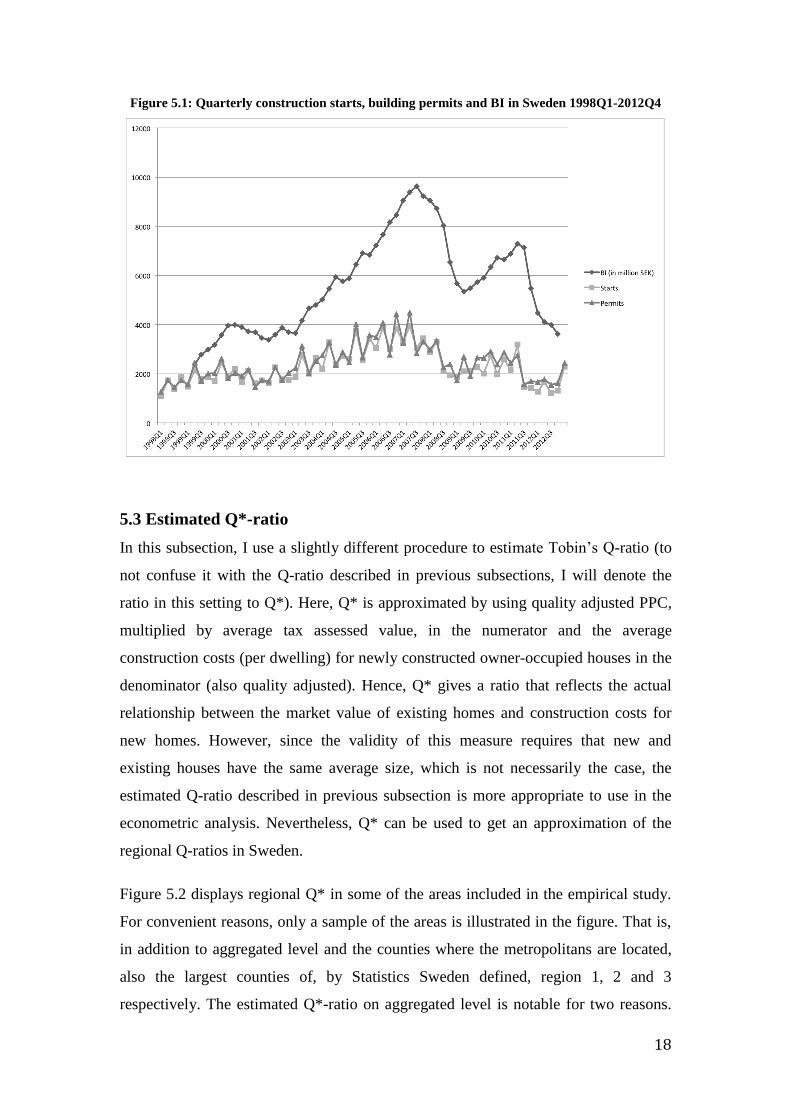
Figure 5.1 displays the estimated building starts, building permits and BI for Sweden

on quarterly level 1998-2012. For convenient reasons, the graph only shows the ratio

on the aggregated level (see Appendix, table A3 for descriptive statistics). From the

figure, it is clear that housing investment, and particularly starts and permits, is

associated with seasonal variation, which motivates the inclusion of seasonal

dummies in the estimated equations. From figure 5.1 one can also see that housing

investment increased from the end 1990s but fell during the global economic

downturn in 2008-2009. After recovering in 2010, starts and permits dropped again in

2011, possibly because of the introduction of a mortgage ceiling in 2010, limiting

mortgage rates to 85% of the market value of the dwelling. In 2012 and 2013 (not

shown in the table) housing investment has partly recovered.

18

Figure 5.1: Quarterly construction starts, building permits and BI in Sweden 1998Q1-2012Q4

5.3 Estimated Q*-ratio

In this subsection, I use a slightly different procedure to estimate Tobin’s Q-ratio (to

not confuse it with the Q-ratio described in previous subsections, I will denote the

ratio in this setting to Q*). Here, Q* is approximated by using quality adjusted PPC,

multiplied by average tax assessed value, in the numerator and the average

construction costs (per dwelling) for newly constructed owner-occupied houses in the

denominator (also quality adjusted). Hence, Q* gives a ratio that reflects the actual

relationship between the market value of existing homes and construction costs for

new homes. However, since the validity of this measure requires that new and

existing houses have the same average size, which is not necessarily the case, the

estimated Q-ratio described in previous subsection is more appropriate to use in the

econometric analysis. Nevertheless, Q* can be used to get an approximation of the

regional Q-ratios in Sweden.

Figure 5.2 displays regional Q* in some of the areas included in the empirical study.

For convenient reasons, only a sample of the areas is illustrated in the figure. That is,

in addition to aggregated level and the counties where the metropolitans are located,

also the largest counties of, by Statistics Sweden defined, region 1, 2 and 3

respectively. The estimated Q*-ratio on aggregated level is notable for two reasons.

19

First, as shown in the figure, Q* is far below equilibrium over the whole time period.

Secondly, the time series is fairly smooth over time, indicating that the production

cost and market value has developed in the same pace. These findings contradict

earlier studies (eg. Berg & Berger, 2006, and Berger, 2000) which, in overlapping

time series, estimates a Q-ratio on the Swedish market that is closer to 1 and also

more volatile. The figure also reveals great difference in Q*-ratios across regions,

both in terms of the magnitude and trend. Stockholm has a Q* that is much higher

than in any other regions, with a ratio above equilibrium in almost all quarters and far

above in most of them.

Figure 5.2: Q*-ratios in selected areas 1998Q1 – 2012Q4

Except Stockholm, no region has a Q* above equilibrium in any time period. Skåne

and Västra Götaland (the counties where Malmö and Gothenburg are located,

respectively) have a higher Q* than their neighbour counties, but still lower than

necessary for housing investment to be profitable. Due to lack of data, it is not

possible to investigate the metropolitan areas of Gothenburg and Malmö separately in

20

this graph, which may have given different results. Västerbotten, in northern Sweden,

has the lowest average Q* in this sample, just over 0,5, indicating that the

construction cost for a new house is twice the market value of existing houses.

The graphs in figure 5.2 may raise the question whether Tobin’s Q can be applied in

the analysis of the Swedish housing market. The theory suggests that there should be

no investment if the Q-ratio is below one, which is the case in all counties except

Stockholm. However, during the observed time period, 77 % of the building starts

have taken place outside Stockholm. Also, if the theory holds, the long run Q-ratio

should converge to equilibrium, which does not seem to be the case.

There are, however, some possible explanations why we see surprisingly low Q*-

ratios overall. First, it is a possible explanation why the investment level has remained

on a low level in recent decades. Second, as already mentioned, this setting assumes

that the size of new and existing houses is the same. If this is not the case, the

estimated ratios are biased upwards or downwards. Third, we do only observe the

county average Q*-ratios, and local differences within a county are not observable.

Hence, even though the average Q* in a county is below zero, it is still possible that

there are local Q*-ratios above equilibrium within the same county. Fourth, and

perhaps most important, new and existing houses may not be perfect substitutes. In

many cases, new houses may have higher quality than existing ones, which makes

buyers willing to pay more for them. If there is a mark-up in the value of newly built

homes, this will, at least partly, explain why the Q*-ratios are below equilibrium in all

regions outside Stockholm.

Unlike the other counties, the Q*-ratio for Stockholm is above equilibrium, indicating

that it is a good return on housing investment in the metropolitan area surrounding the

capital of Sweden. The Q theory claims that, if the Q-ratio is above 1, the investment

will increase until the market reaches equilibrium. However, increasing demand on

housing during the last decades, due to high urbanisation, combined with regulations

on the supply side, making it difficult for producers to receive building permits, are

two possible explanations of the high Q*-ratio in Stockholm.

An important learning from figure 5.2 is that the regional Q*-ratios differs remarkably

from the aggregated level, both when it comes to magnitude and trend. If conducting

21

an analysis on disaggregated level, rather than aggregated, regional effects are taken

into account. Consequently, the existence of regional variation in Tobin’s Q implies

that analysis on regional level is a relevant contribution to the literature.

6. Results

This section presents the estimated results of the econometric analysis. In subsection

6.1-6.4, the outcome of Johansen’s LM procedure is presented. In subsection 6.5, an

alternative model is estimated, by transforming the VECM into an autoregressive

distributed lag (ARDL) model. In subsection 6.6, two-way causality is examined for

using the Granger-Causality test. In the final subsection, 6.7, regional panel data is

used to investigate whether the explanatory power of the model is stronger when

using disaggregated data.

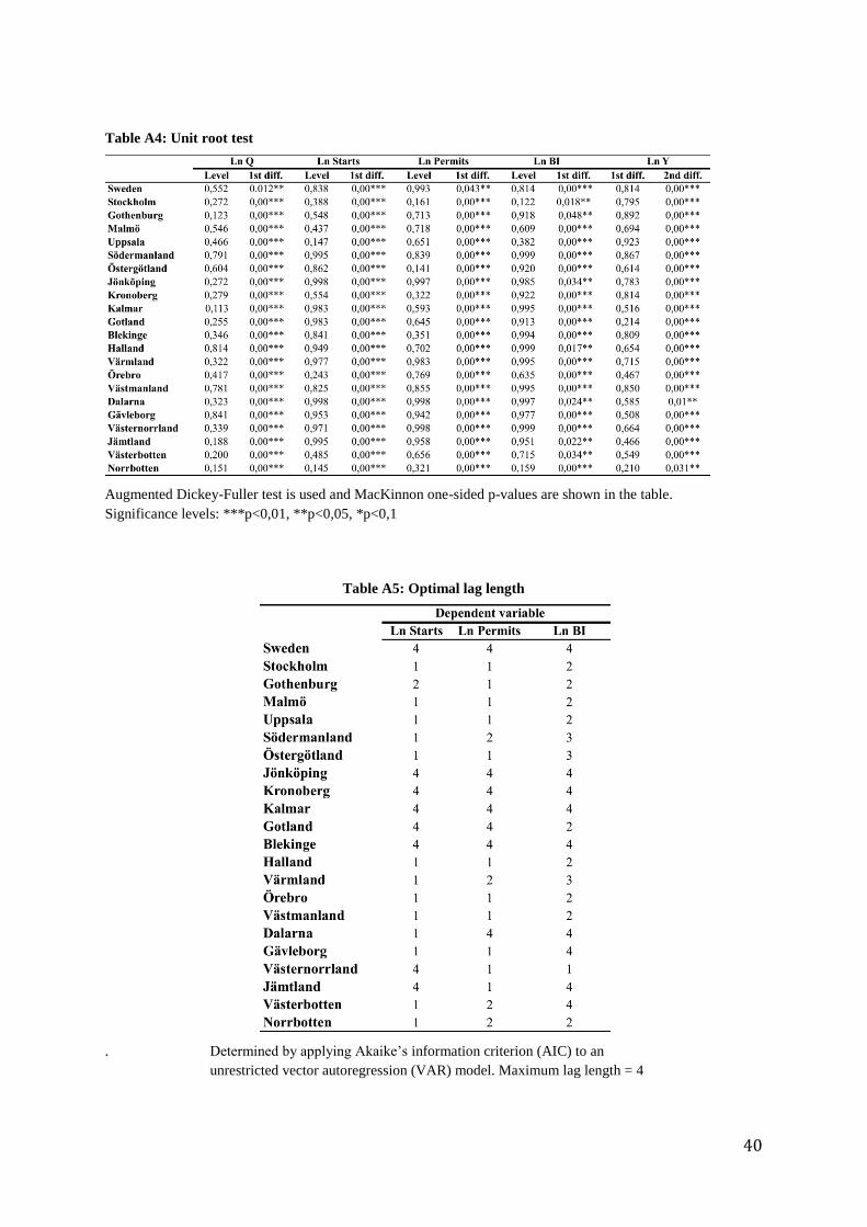
6.1 Unit root test

The Augmented Dickey Fuller test, summarized in table A4 in Appendix, consists to

what have been found in earlier studies. That is, investment, regardless which proxy

that is used, and the Q-ratio are integrated of order one, I(1). That is, these variables

are found to be non-stationary in levels but stationary in first differenced form for all

areas. However, income is found to be non-stationary in first differenced form but

stationary in second difference, i.e. I(2), for all areas. As a consequence, since co-

integration requires integration of the same order (Gujterati and Porter, 2009), for the

further analysis I need to difference income one additional time to make its time

series I(1). The additional differentiation of income will not affect the analysis since it

is the relationship between investment and Q that is of main interest. It will, however,

make the income coefficients less interesting for economic interpretation.

6.2 Optimal lag structure

Table A5 in Appendix displays the lag length that is used for each equation, found by

estimating an unrestricted VAR model and use AIC to determine the optimal lag

structure. As mentioned above, the maximum lag length is set to four quarters. As can

be seen in table A5, there is a huge variation in optimal lag length across different

22

regions. For instance, the counties in southern Sweden have a higher average lag

length compared to the remaining regions, irrespective of which dependent variable

that is used. Notably, the metropolitan areas all have a relatively short lag length, not

exceeding two for any of the dependent variables. On aggregated level, the suggested

lag length is four for all investment variables.

Since the three investment variables captures different dynamics of housing

investment (as discussed in subsection 4.1, I expected greater difference between

them in terms of average lag length. In particular, I expected the equations with BI as

dependent variable to have longer lag length than the equations where starts and

permits are used. However, the average lag length is essentially the same for all three

dependent variables.

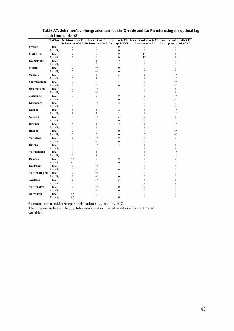
6.3 Johansen’s co-integration test

Table A6-A8 in Appendix displays the outcome of Johansen’s co-integration test. As

have already been mentioned, AIC is used to identify the optimal specification of the

test in terms of coefficients and time trend in co-integrated equation and the VAR.

The integers in the tables show the estimated numbers of co-integrated equations. At

least one co-integrated equation is necessary for the VECM to be used. I find co-

integration between Q and at least one investment variable in 14 counties and

metropolitan areas. Only in three counties (Uppsala, Kalmar and Gotland), I find co-

integration between Q and all investment variables. In seven counties, no co-

integrated vector is found for any of the three investment variables.

It is hard to discern any patterns for the co-integration test. For instance, the test

results for the metropolitan areas do not stand out from the other regions.

Furthermore, there is a great difference in, by AIC, suggested trend and intercept

specification. Both between different counties and within the same county, depending

on which investment variable that is used. On the aggregated level, co-integration is

only found between Q and BI. This contradicts the findings by Berg and Berger

(2006), who found co-integration between Q and starts but not between Q and

estimated gross investment.

23

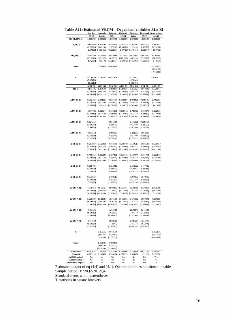
6.4 Vector error correction model (VECM)

Table 6.1 and 6.2 summarize the long run and the short run relationship between Q

and housing investment for different counties (In table A9-A11 in Appendix, the

complete models are presented). Note that the VECM is only computed on those

equations that were found to be stationary above. Table 6.1 displays the long run

supply elasticity of housing investment with respect to the Q-ratio. That is, the

estimated percentages increase in housing investment when the Q-ratio increases by 1

%. For instance, if the house prices in Stockholm increase by 1 %, relative to

construction costs, the estimated increase in building starts is 2,68%.

As can be seen from the table, for all counties and metropolitan areas where at least

one investment variable passed the co-integration test, the Q-ratio has a significant

long run impact at 1% level on at least one investment variable. This is also the case

on aggregated level. For Kalmar and Gotland counties, the long run relationship is

significant on 1 % level for all investment variables. As can also be seen from the

table, some of the long run estimates are remarkably large. The explanation why some

long run estimates are much larger is the exclusion of an intercept in these co-

integrated equations. In other word, exclusion of an intercept in eq. (4.4) leads to

larger point estimates. To obtain more realistic results, it would have been preferable

to include an intercept in these co-integrated equations. However, since these are the

specifications suggested by AIC, I will stick to it even though it is unrealistic that a 1

% rise in Q increases investment by 40-50%. Instead, one should focus on the

significance of the coefficient rather than the magnitude.

From table A9-A11 in Appendix, one can see that there is a significant error

correction mechanism in 15 out of 28 estimated VECM equations. On aggregated

level, this mechanism is insignificant for BI. For the metropolitans, the mechanism is

significant in Stockholm for both starts and permits but insignificant for both

variables in Gothenburg.

24

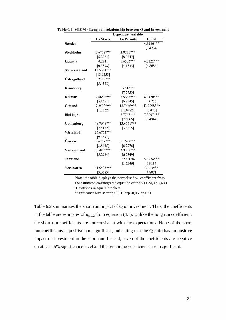
Table 6.1: VECM - Long run relationship between Q and investment

Note: the table displays the normalised -coefficient from

the estimated co-integrated equation of the VECM, eq. (4.4).

T-statistics in square brackets.

Significance levels: ***p<0,01, **p<0,05, *p<0,1

Table 6.2 summarizes the short run impact of Q on investment. Thus, the coefficients

in the table are estimates of from equation (4.1). Unlike the long run coefficient,

the short run coefficients are not consistent with the expectations. None of the short

run coefficients is positive and significant, indicating that the Q-ratio has no positive

impact on investment in the short run. Instead, seven of the coefficients are negative

on at least 5% significance level and the remaining coefficients are insignificant.

25

Table 6.2: VECM – Short run relationship between Q and investment

Note: the table displays the -coefficients from the estimated VECM, eq. (4.1).

T-statistics in square brackets.

Significance levels: ***p<0,01, **p<0,05, *p<0,1

The LM and the Jarque Bera tests, shown in table A9-A11, suggests that

autocorrelation exists in about 1/3 of the equations while heteroscedasticity is a main

problem in this setting. The outcome of these tests makes it even more relevant to use

an alternative model to verify the results.

To summarize the outcome of the VECM, I find evidence that the impact of Q on

investment is consistent with theory in the long run but inconsistent in the short run. It

may seem confusing that the Q-ratio could have a positive impact in the long run but

negative impact in the short run. However, one possible explanation is that, in the

short run, the mechanisms that affects investment are more difficult to capture by

Tobin’s Q. Thus, even though a long run impact exists, it may not be visible in the

short run.

26

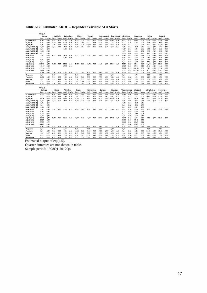
6.5 Autoregressive distributed Lag (ARDL) model

The ARDL model is conducted as an alternative model to Johansen’s LM procedure.

The model is estimated on aggregated level and for all counties and metropolitan

areas. In the estimated equations, I use the lag structure found in subsection 6.2.

The outcome of the Wald test is summarized in table 6.3. The Wald test acts as an

alternative test to Johansen’s co-integration test presented above. The test is

conducted by simply testing the joint impact of the lagged level variables in the

estimated ARDL equations. If the coefficients are jointly differenced from zero, one

concludes that co-integration exists (Pesaran et al., 2001).

Table 6.3: Co-integration test (using Wald test)

Note: The table displays Wald’s F-statistics when testing the

following null hypothesis: on eq (4.5)

Significance levels: ***p<0,01, **p<0,05, *p<0,1

As can be seen from table 6.3, when using the Wald test instead of Johansen’s test,

there are fewer co-integrated equations found. However, the outcome of the two tests

is rather similar overall, since there are only a few cases where co-integration is found

by the Wald test but not by Johansen’s test. Just like in the Johansen test, I find strong

27

evidence of co-integration in the counties of Uppsala and Gotland. Unlike in

Johansen’s test, the Wald test finds co-integration for Gävleborg county. Also, the

Wald test suggests co-integration for all dependent variables in Kronoberg county.

However, I do not find co-integration between Q and aggregated investment since

none of these tests reject the null hypothesis. This, together with the results found in

the last subsection, suggests that the explanatory power of Q is weak when using

aggregated data.

Table 6.4: ARDL – Long run relationship between Q and investment

Note: The table displays the normalized -coefficients from

the estimated ARDL-model, eq (4.5)

P-values within parentheses

Significance levels: ***p<0,01, **p<0,05, *p<0,1

28

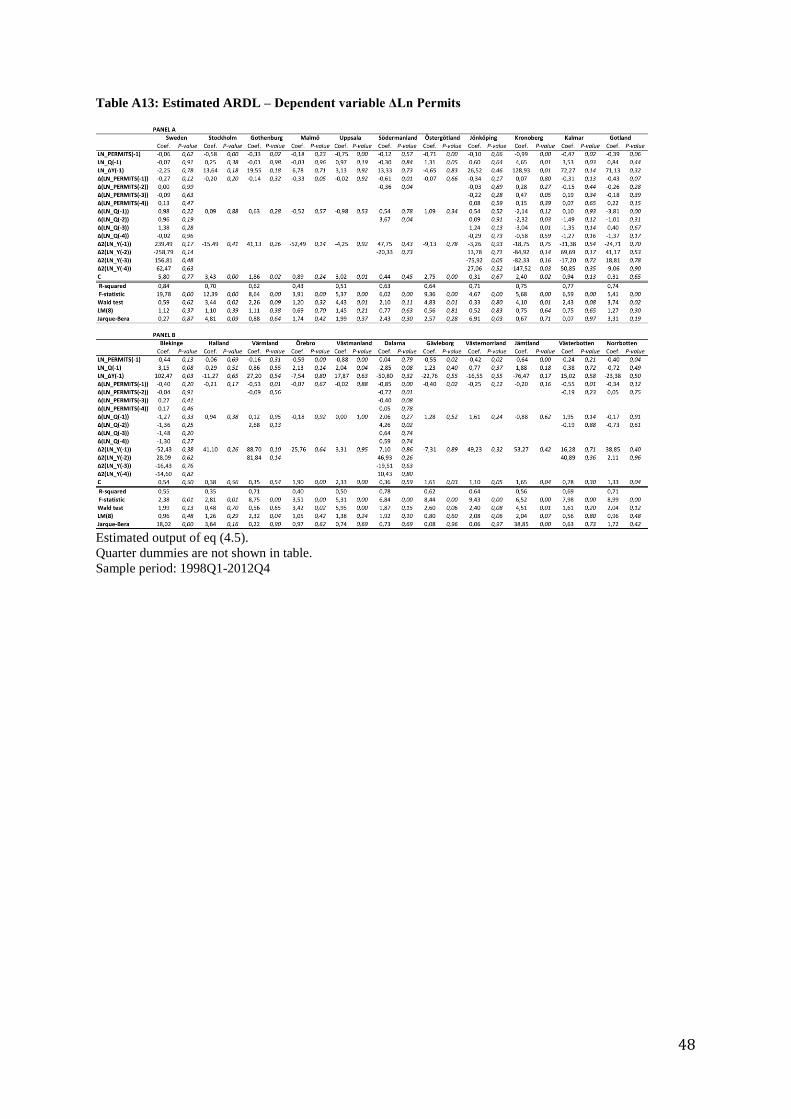
In table 6.4 and 6.5, I present the long run- and short run estimates for those areas

where co-integration was found in the Wald test on at least 10% level (table A12-A14

in Appendix displays all estimated ARDL models, also for those areas where no co-

integration was found). The long run coefficients in table 6.4 are obtained by

normalizing the coefficient of with respect to the coefficient of by

following the procedure of Pesaran et al. (2001). As can be seen from table 6.4,

significant coefficients are only found in five counties. Also, unlike my expectations,

I do not find long run impact of Q in any of the metropolitans. Hence, this indicates

that the correlation between Q and investment is not stronger in the metropolitan

areas. Moreover, Table A12-A14 in Appendix show that the error correction

mechanism is significant in nearly all cases where co-integration is found, suggesting

that regional investment adjusts to equilibrium after a change in Q or income.

29

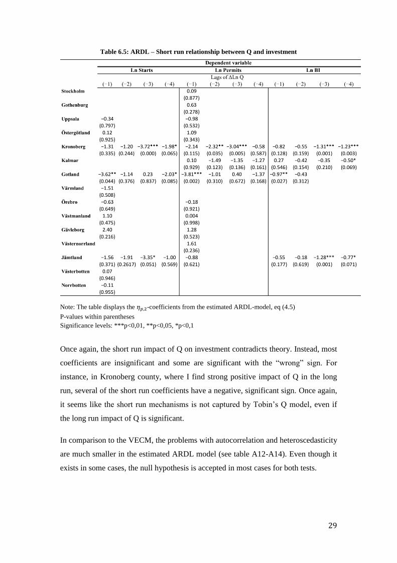
Table 6.5: ARDL – Short run relationship between Q and investment

Note: The table displays the -coefficients from the estimated ARDL-model, eq (4.5)

P-values within parentheses

Significance levels: ***p<0,01, **p<0,05, *p<0,1

Once again, the short run impact of Q on investment contradicts theory. Instead, most

coefficients are insignificant and some are significant with the “wrong” sign. For

instance, in Kronoberg county, where I find strong positive impact of Q in the long

run, several of the short run coefficients have a negative, significant sign. Once again,

it seems like the short run mechanisms is not captured by Tobin’s Q model, even if

the long run impact of Q is significant.

In comparison to the VECM, the problems with autocorrelation and heteroscedasticity

are much smaller in the estimated ARDL model (see table A12-A14). Even though it

exists in some cases, the null hypothesis is accepted in most cases for both tests.

30

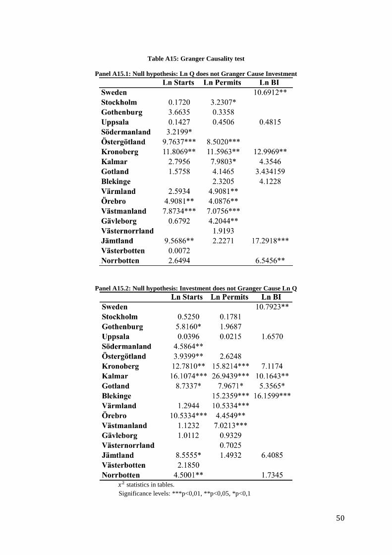
6.6 Granger Causality test

It is a general fact that two-way causality is common in economic relationships. In

this subsection, I will use the Granger causality test to investigate whether the

estimated models are associated with two-way causality.

In a general supply function, price and quantity is simultaneously determined. That is,

the price affects supplied quantity but the supplied quantity also affects price.

Applying this theory on the housing market implies that housing investment and the

Q-ratio might be determined simultaneously. In fact, the theory actually states that

housing investment and Q is simultaneously determined. That is, recalling from the

theoretical discussion in section 3, an increase in housing investment, due to a price

shock that raises Q from its equilibrium level, will dampen the market price and move

Q back to equilibrium.

Among earlier studies on this topic, it does not seem to be common practice to test if

two-way causality is present, even though the theory suggests that it exists. However,

a common explanation (see eg. Takala and Toumala, 1991; Jud and Winkler, 2003)

why Q should be exogenous to investment is that new houses only represents a small

proportion of the total housing stock. Thus, investment does not affect prices. Barot

and Yang (2002), however, conducted the Granger causality test on the Swedish and

British housing market. In neither of the cases, they found Granger causality of

investment on the Q-ratio.

The test is conducted by estimation of an unrestricted VAR model and test for

causality, using the same lag structure as found in subsection 6.2. By doing that, I test

for the two-way causality of investment and Q, while taking the effects of income into

account. I have only computed the test for those equations where I have found co-

integration. Note that I am only investigating the Granger causality between

investment and Q since this is the relationship of main interest.

Table A15 in Appendix summarizes the Granger Causality tests. As can be seen from

the table, there is no clear causal direction in the relationship between investment and

Q. Instead, I find several cases of simultaneous impact. Furthermore, in some cases,

the causal impact is only significant in the “wrong” direction. These results show that,

when investigating the relationship between Q and investment, one have to be aware

31

that two-way causality may exist, causing endogeneity problem. Adding more control

variables or use instrumental variables for Q may be the best way to improve the

specification of the model and, thus, get rid of the endogeneity problem.

6.7 Fixed Effects model

The estimated panel data regressions with county fixed effects are displayed in table

6.6. As can be seen from the table, I find positive significant impact of Q on

investment, regardless of which dependent variable that is used.

Table 6.6: Estimated Fixed Effects model

Estimation output of eq (4.6)

Sample period: 1998Q1-2012Q4 (Note: 1999Q2-2012Q4 for Ln BI)

T-statistics in square brackets

Significance levels: ***p<0,01, **p<0,05, *p<0,1

The fixed effects model estimates suggest that the long run supply of housing

investment is inelastic with respect to Q, since a 1 % increase in house prices, relative

to construction costs, just increase investment by 0,53-0,69 % depending on which

dependent variable that is used. These long run elasticities are low compared to what

was found in the estimated VECM on aggregated data, which suggested 4,7 %

elasticity in BI with respect to Q. Moreover, these estimates are also low compared to

the elasticities found by earlier studies on Swedish aggregated data. Barot and Yang

(2002) found a long run supply elasticity of 2,8% and Berg and Berger (2006)

suggested 6,5%.

32

When comparing the results from table 6.6 to the results found on aggregated data in

previous subsections, one can see that, when using panel data instead of aggregated,

the correlation between Q and investment is improved. Moreover, the adjusted R-

squares (not shown in tables for estimated VECM and ARDL equations) are

substantially higher in the fixed effects models than in the VECM and ARDL

equations on aggregated data. These findings suggest that, using disaggregated data

rather than aggregated data improves the explanatory power of the model.

7. Concluding remarks

The objectives of this thesis was (1) to investigate the relationship between Tobin’s Q

and regional housing investment in Sweden and (2) to examine the gain in

explanatory power from using disaggregated data rather than aggregated in the model.

The results found by the VECM suggest a long run positive relationship between Q

and at least one of the investment variables in 14 out of 21 investigated counties and

metropolitan areas on 1 % level, as well as a long run relationship between Q and BI

on aggregated level. The ARDL model, however, does only find a long run impact of

Q on BI in five of the counties on 5 % level, while no long run impact is found in

neither the metropolitan areas nor on the aggregated level. For the short run impact of

Q, both the VECM and the ARDL model receives either insignificant or even

negative estimates. These findings suggest that, even if Q and investment have a

positive correlation in the long run, Tobin’s Q model does not seem to capture the

short run dynamics of housing investment. From these results, it is obvious that the

correlation between Q and investment is not stronger in the metropolitan areas

compared to the other counties. However, a further investigation is required before

one can draw any definite conclusion about this.

When estimating the aggregated relationship between Q and investment using panel

data, I find strongly significant long run relationships between Q and all investment

variables. In comparison to the VECM and the ARDL model on aggregated data, the

fixed effects model does not only yields more significant correlation between Q and

investment, but also substantially higher adjusted coefficients of determination. These

findings suggest that the explanatory power of Q increases when disaggregated data is

33

used rather than aggregated. That is, when investigating the relationship between Q

and housing investment on national level, a researcher may improve the precision of

the estimates by taking regional effects into account.

The Granger Causality test indicates that a two-way causality exists between Tobin’s

Q and investment. The presence of two-way causality will cause endogeneity

problems in the estimated equations, making the coefficients biased and inconsistent.

Future researchers on this topic may try to get rid of the endogeneity problem, and

hence get consistent estimates, by improving the specification of the model. For

instance, adding more control variables or using instrumental variables for Q could be

two possible solutions.

A potential topic for future research would be to go more deeply into the analysis of

the differences between urban and rural housing markets regarding the relationship

between Q and investment. This will, however, require data on smaller areas than

what is used in this thesis. Another potential topic for the Swedish housing market

would be to include structural breaks to control for the financial crisis in 2008 and the

introduction of the mortgage ceiling in 2010, limiting the mortgage rate to 85 % of the

market value of the dwelling. Since these two events decreased housing investment

they may also have affected the correlation between Q and investment.

34

List of references Abel, A. B. (1980). Empirical investment equations: An integrative framework.

In Carnegie-Rochester Conference Series on Public Policy (Vol. 12, pp. 39-91).

North-Holland.

Banerjee, A., Dolado, J. J., Galbraith, J. W., & Hendry, D. (1993). Co-integration,

error correction, and the econometric analysis of non-stationary data. Oxford: Oxford

University Press.

Barot, B., & Yang, Z. (2002). House prices and housing investment in Sweden and

the UK: Econometric analysis for the period 1970–1998. Review of Urban &

Regional Development Studies, 14(2), 189-216.

Berg, L., & Berger, T. (2006). The Q theory and the Swedish housing market—an

empirical test. The Journal of Real Estate Finance and Economics, 33(4), 329-344.

Berger, T. (1998). Priser på egenskaper hos småhus. Institutet för bostadsforskning,

Uppsala universitet, Arbetsrapport/Working Paper, (14).

Berger, T. (2000). Tobins q på småhusmarknader (Tobin's q on markets for single-

family houses). Prisbildning och värdering av fastigheter. Var står svensk forskning

inför 2000-talet? En antologi om svensk bostadsekonomisk forskning.

Boverket (2013). Are house prices driven by a housing shortage? Market report.

February. [online]

Available at:

http://www.boverket.se/Global/Webbokhandel/Dokument/2013/Are-house-prices-

driven-by-a-housing-shortage.pdf [Accessed: 24 May 2014]

Engle, R. F., & Granger, C. W. (1987). Co-integration and error correction:

representation, estimation, and testing. Econometrica: journal of the Econometric

Society, 251-276.

Fettig, D. (1996). “Interview with James Tobin.” Federal Reserve bank of

Minneapolis, The Region 10, 1-15.

Grimes, A., & Aitken, A. (2010). Housing supply, land costs and price

adjustment. Real Estate Economics, 38(2), 325-353.

Gujarati, D. N., & Porter, D. C. (2009). Basic Econometrics (Fifth Edition ed.). New

York: McGraw-Hill Book Company

Hayashi, F. (1982), Tobin’s Marginal, Q., & Average, Q. A Neoclassical

Interpretation. Econometrica, 50, 731-753.

35

Jaffee, D. M. (1994). Den svenska fastighetskrisen (The Swedish Real Estate Crisis).

Stockholm: SNS Förlag.

Johansen, S. (1988). Statistical analysis of cointegration vectors. Journal of economic

dynamics and control, 12(2), 231-254.

Johansen, S. (1991). Estimation and hypothesis testing of cointegration vectors in

Gaussian vector autoregressive models. Econometrica: Journal of the Econometric

Society, 1551-1580.

Johansen, S. (1995). Likelihood-based Inference in Cointegrated Vector

Autoregressive Models, Oxford University Press: Oxford

Jud, G. D., & Winkler, D. T. (2003). The Q theory of housing investment. The

Journal of Real Estate Finance and Economics, 27(3), 379-392.

Kydland, F. E., & Prescott, E. C. (1982). Time to build and aggregate

fluctuations. Econometrica: Journal of the Econometric Society, 1345-1370.

Mankiw. N.G & Taylor, M.P (2008), Macroeconomics. European edition. New York:

Worth Publishers.

Mayer, C.J. and C.T. Somerville (2000). Residential Construction: Using the Urban

Growth Model to Estimate Housing Supply. Journal of Urban Economics 48(1): 85–

109.

Meese, R., & Wallace, N. (1994). Testing the present value relation for housing

prices: Should I leave my house in San Francisco?. Journal of urban

economics, 35(3), 245-266.

Narayan, P. K. (2004). Reformulating critical values for the bounds F-statistics

approach to cointegration: an application to the tourism demand model for Fiji.

Monash University.

Pesaran, M. H., Shin, Y., & Smith, R. J. (2001). Bounds testing approaches to the

analysis of level relationships. Journal of applied econometrics, 16(3), 289-326.

Romer, D. (2011), Advanced Macroeconomics. 4th edition. New York: McGraw-Hill.

Summers, L. H. (1980). Inflation, Taxation, and Corporate Investment: A q-Theory

Approach (No. 0604). National Bureau of Economic Research, Inc.

Statistics Sweden/SCB (2004), SCB-indikatorer, nr 1, 3 feb. [Online]

Available at:

http://www.scb.se/sv_/Hitta-statistik/Temaomraden/Sveriges-

ekonomi/Konjunkturen/SCB-Indikatorer/ [Accessed: 5 May 2014]

36

Takala, K., & Tuomala, M. (1990). Housing investment in Finland. Finnish Economic

Papers, 3(1), 41-53.

Tobin, J. (1969). A general equilibrium approach to monetary theory. Journal of

money, credit and banking, 1(1), 15-29.

Topel, R., & Rosen, S. (1988). Housing investment in the United States. The Journal

of Political Economy, 718-740.

37

Appendix

Figure A1: Scatter plots of the logarithms for building starts, building permits and BI and the Q-

ratio for owner-occupied houses for Swedish national, aggregated data. Trend lines are included

for descriptive purposes.

Panel A1.1. LN (Starts) vs. Q-ratio. 1998Q1-2012Q4

Panel A1.2. LN (Permits) vs. Q-ratio. 1998Q1-2012Q4

Panel A1.3. LN (BI) vs. Q-ratio. 1999Q2-2012Q4

38

Table A1: Regional subdivision

Table A2: Data appendix

All data is collected from Statistics Sweden

39

Table A3: Descriptive Statistics

See subsection 5.3 for definition of Q*

* Skåne county, ** Västra Götaland county

40

Table A4: Unit root test

Augmented Dickey-Fuller test is used and MacKinnon one-sided p-values are shown in the table.

Significance levels: ***p<0,01, **p<0,05, *p<0,1

Table A5: Optimal lag length

. Determined by applying Akaike’s information criterion (AIC) to an

unrestricted vector autoregression (VAR) model. Maximum lag length = 4

41

Table A6: Johansen’s co-integration test for the Q-ratio and LN Starts using the optimal lag

length from table A5

* denotes the trend/intercept specification suggested by AIC. The integers indicates the, by Johansen’s test

estimated number of co-integrated variables.

42

Table A7: Johansen’s co-integration test for the Q-ratio and Ln Permits using the optimal lag

length from table A5

* denotes the trend/intercept specification suggested by AIC.

The integers indicates the, by Johansen’s test estimated number of co-integrated

variables

43

Table A8: Johansen’s co-integration test for the Q-ratio and Ln BI

using the optimal lag length from table A5

* denotes the trend/intercept specification suggested by AIC.

The integers indicates the, by Johansen’s test estimated number of co-integrated

variables.

44

Table A9: Estimated VECM – Dependent variable: ΔLn Starts

Estimated output of eq (4.4) and (4.1). Quarter dummies not shown in table

Sample period: 1998Q1-2012Q4

Standard errors within parentheses

T-statistics in square brackets

45

Table A10: Estimated VECM – Dependent variable: ΔLn Permits

Estimated output of eq (4.4) and (4.1). Quarter dummies not shown in table

Sample period: 1998Q1-2012Q4

Standard errors within parentheses

T-statistics in square brackets

46

Table A11: Estimated VECM – Dependent variable: ΔLn BI

Estimated output of eq (4.4) and (4.1). Quarter dummies not shown in table

Sample period: 1999Q2-2012Q4

Standard errors within parentheses

T-statistics in square brackets

47

Table A12: Estimated ARDL – Dependent variable ΔLn Starts

Estimated output of eq (4.5).

Quarter dummies are not shown in table.

Sample period: 1998Q1-2012Q4

48

Table A13: Estimated ARDL – Dependent variable ΔLn Permits

Estimated output of eq (4.5).

Quarter dummies are not shown in table.

Sample period: 1998Q1-2012Q4

49

Table A14: Estimated ARDL – Dependent variable ΔLn BI

Estimated output of eq (4.5).

Quarter dummies are not shown in table.

Sample period: 1999Q2-2012Q4

50

Table A15: Granger Causality test

Panel A15.1: Null hypothesis: Ln Q does not Granger Cause Investment

Panel A15.2: Null hypothesis: Investment does not Granger Cause Ln Q

statistics in tables.

Significance levels: ***p<0,01, **p<0,05, *p<0,1