tmap 2.0 user's guide - fm 2.0 user’s guide maurizio pisati department of sociology and...

tmap 2.0 User’s guide

Maurizio Pisati

Department of Sociology and Social Research University of Milano Bicocca, Italy

[email protected] 1 Introduction

The tmap package is a suite of Stata programs designed to carry out simple thematic mapping. The first public release of tmap (1.2) was described in the latest issue of The Stata Journal (Pisati 2004). The purpose of this document is to offer a hands-on introduction to the second public release of tmap (2.0) which, thanks to Kit Baum, is available from the SSC archive. For the sake of parsimony, in the following I will assume that the reader is already familiar with the first public release of tmap.

Section 2 illustrates the syntax of the new release of tmap. To facilitate the existing users of tmap, new options are indicated in blue, while revised options are indicated in red.

To exploit tmap, the user must be able to access geographical boundary files in the proper format. Section 3 illustrates the format adopted by the new release of tmap, shows how to adapt the existing boundary files to the current format, and presents mif2dta, a Stata program that converts MapInfo Interchange Format boundary files into Stata boundary files to be used with the new release of tmap.

Finally, section 4 illustrates the new features of tmap by examples. 2 The tmap package 2.1 Syntax tmap choropleth quantvar [if exp] [in range], id(varname) map(filename)

[ clmethod(quantile | eqint | stdev | custom | unique) clnumber(#) clbreaks(numlist) eirange(numlist) palette(colorscheme) colors(colorstyle_list) ocolor(colorstyle) osize(linewidthstyle) bcolor(colorstyle) title(tinfo) subtitle(tinfo) note(tinfo) caption(tinfo) legpos(#) legcolor(colorstyle) legsize(#) legformat(format) legtitle(tinfo) legbox(roptions) legcount nolegend addplot(command) ]

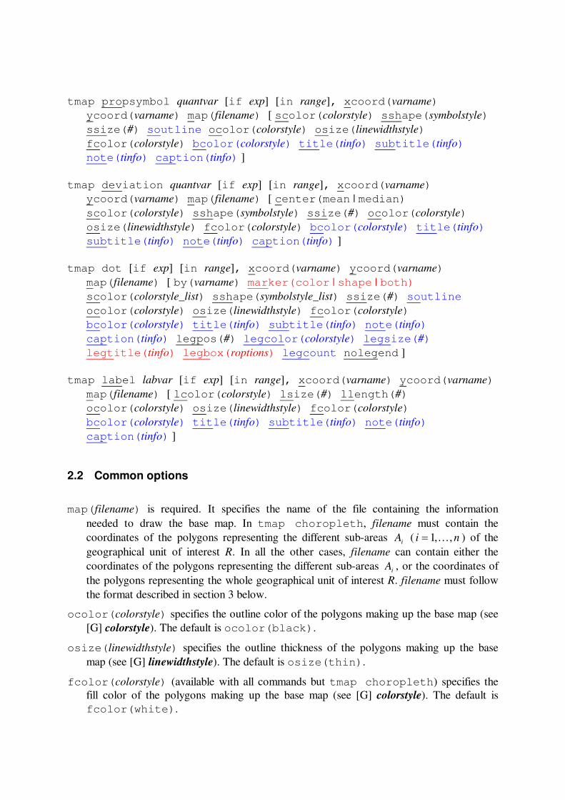
tmap propsymbol quantvar [if exp] [in range], xcoord(varname) ycoord(varname) map(filename) [ scolor(colorstyle) sshape(symbolstyle) ssize(#) soutline ocolor(colorstyle) osize(linewidthstyle) fcolor(colorstyle) bcolor(colorstyle) title(tinfo) subtitle(tinfo) note(tinfo) caption(tinfo) ]

tmap deviation quantvar [if exp] [in range], xcoord(varname)

ycoord(varname) map(filename) [ center(mean | median) scolor(colorstyle) sshape(symbolstyle) ssize(#) ocolor(colorstyle) osize(linewidthstyle) fcolor(colorstyle) bcolor(colorstyle) title(tinfo) subtitle(tinfo) note(tinfo) caption(tinfo) ]

tmap dot [if exp] [in range], xcoord(varname) ycoord(varname)

map(filename) [ by(varname) marker(color | shape | both) scolor(colorstyle_list) sshape(symbolstyle_list) ssize(#) soutline ocolor(colorstyle) osize(linewidthstyle) fcolor(colorstyle) bcolor(colorstyle) title(tinfo) subtitle(tinfo) note(tinfo) caption(tinfo) legpos(#) legcolor(colorstyle) legsize(#) legtitle(tinfo) legbox(roptions) legcount nolegend ]

tmap label labvar [if exp] [in range], xcoord(varname) ycoord(varname)

map(filename) [ lcolor(colorstyle) lsize(#) llength(#) ocolor(colorstyle) osize(linewidthstyle) fcolor(colorstyle) bcolor(colorstyle) title(tinfo) subtitle(tinfo) note(tinfo) caption(tinfo) ]

2.2 Common options

map(filename) is required. It specifies the name of the file containing the information needed to draw the base map. In tmap choropleth, filename must contain the coordinates of the polygons representing the different sub-areas iA ( ni ,,1� ) of the geographical unit of interest R. In all the other cases, filename can contain either the coordinates of the polygons representing the different sub-areas iA , or the coordinates of the polygons representing the whole geographical unit of interest R. filename must follow the format described in section 3 below.

ocolor(colorstyle) specifies the outline color of the polygons making up the base map (see [G] colorstyle). The default is ocolor(black).

osize(linewidthstyle) specifies the outline thickness of the polygons making up the base map (see [G] linewidthstyle). The default is osize(thin).

fcolor(colorstyle) (available with all commands but tmap choropleth) specifies the fill color of the polygons making up the base map (see [G] colorstyle). The default is fcolor(white).

bcolor(colorstyle) specifies the background color of the graph (see [G] colorstyle). The default is bcolor(white).

title(tinfo) specifies the overall title of the graph (see [G] title_options).

subtitle(tinfo) specifies the subtitle of the graph (see [G] title_options).

note(tinfo) specifies notes to be displayed with the graph (see [G] title_options).

caption(tinfo) specifies an explanation to accompany the graph (see [G] title_options). 2.3 Options for tmap choropleth

id(varname) is required. It specifies the name of the numeric variable that uniquely identifies the different sub-areas iA of the geographical unit of interest R. The values taken on by varname must correspond to the values taken on by the identifier _ID contained in the file specified with option map(filename).

clmethod(quantile | eqint | stdev | custom | unique) specifies the method to be used for determining the class breaks.

clmethod(quantile) is the default and requests that the quantiles method be used.

clmethod(eqint) requests that the equal intervals method be used.

clmethod(stdev) requests that the standard deviates method be used.

clmethod(custom) requests that class breaks be specified by the user with option clbreaks(numlist).

clmethod(unique) requests that the variable of interest quantvar be treated as a categorical variable taking on a maximum of nine different values.

clnumber(#) specifies the number of classes k in which the variable of interest quantvar should be divided. This option accepts only numbers between 2 and 9. The default is clnumber(4).

clbreaks(numlist) is required if option clmethod(custom) is specified. It specifies a list of numbers defined as follows: the first element of the list is the minimum value of quantvar to be considered; the second to kth elements of the list are the class breaks; the last element of the list is the maximum value of quantvar to be considered. For example, suppose that we want to divide the values of quantvar into the following four classes:

]15,10[ , ]20,15( , ]25,20( , and ]50,25( ; for this we must specify clbreaks(10 15 20 25 50).

eirange(numlist) specifies the range of values (minimum and maximum) to be considered in the calculation of class breaks when option clmethod(eqint) is specified. This option overrides the default range )]max(),[min( quantvarquantvar .

palette(colorscheme) specifies the color scheme to be used for representing the different classes in which quantvar has been divided. colorscheme is one of the following:

Blues BrBG Greens Greys Paired PuRd Purples RdBu RdGy Reds Set1 Set3 YlOrBr Custom

The default is palette(Greys) when clmethod(quantile) or clmethod(eqint) is specified; palette(RdBu) when clmethod(stdev) is specified; and palette(Paired) when clmethod(unique) is specified. If option palette(Custom) is specified, option colors(colorstyle_list) must be specified as well.

colors(colorstyle_list) specifies a custom list of colors to be used for representing the different classes in which quantvar has been divided (see [G] colorstyle). The number of elements of the list must equal k, i.e., the desired number of classes.

legpos(clockpos) specifies the position of the map legend (see [G] clockpos). The default is legpos(7).

legcolor(colorstyle) specifies the color of the main text of the map legend (see [G] colorstyle). The default is legcolor(black).

legsize(#) specifies a multiplier that affects the size of the main text of the map legend. For example, to increase the default size of the text by 50%, specify legsize(1.5). The default is legsize(1).

legformat(format) specifies the format of the numeric values appearing in the main text of the map legend (see [U] 15.5 Formats: controlling how data are displayed). The default is legformat(%8.2f).

legtitle(tinfo) specifies the title of the map legend (see [G] title_options). By default, no title is used.

legbox(roptions) requests that a box be drawn around the map legend and specifies its appearance (see [G] legend_option).

legcount requests that the number of sub-areas iA belonging to each class k in which quantvar has been divided be displayed in the map legend.

nolegend requests that the map legend be suppressed.

addplot(command) requests that a propsymbol, deviation, dot or label plot be superimposed onto the current choropleth map. command is one of the following:

propsymbol quantvar [if exp] [in range], xcoord(varname) ycoord(varname) [ scolor(colorstyle) sshape(symbolstyle) ssize(#) soutline ]

deviation quantvar [if exp] [in range], xcoord(varname) ycoord(varname) [ center(mean | median) scolor(colorstyle) sshape(symbolstyle) ssize(#) ]

dot [if exp] [in range], xcoord(varname) ycoord(varname) [ by(varname) marker(color | shape | both) scolor(colorstyle_list) sshape(symbolstyle_list) ssize(#) soutline ]

label labvar [if exp] [in range], xcoord(varname) ycoord(varname) [ lcolor(colorstyle) lsize(#) llength(#)]

2.4 Options for tmap propsymbol

xcoord(varname) is required. It specifies the name of the variable containing the x-coordinate of the centroid of each sub-area iA . varname must be expressed in the same units as the x-coordinates of the polygons making up the base map specified with option map(filename).

ycoord(varname) is required. It specifies the name of the variable containing the y-coordinate of the centroid of each sub-area iA . varname must be expressed in the same units as the y-coordinates of the polygons making up the base map specified with option map(filename).

scolor(colorstyle) specifies the color of the symbols (see [G] colorstyle). The default is scolor(black).

sshape(symbolstyle) specifies the shape of the symbols (see [G] symbolstyle). The default is sshape(Oh), i.e., a hollow circle.

ssize(#) specifies a multiplier that affects the size of the symbols. For example, to increase the size of all the symbols by 50%, specify ssize(1.5). The default is ssize(1).

soutline requests that the symbols be drawn with a black outline. 2.5 Options for tmap deviation

xcoord(varname) is required. It specifies the name of the variable containing the x-coordinate of the centroid of each sub-area iA . varname must be expressed in the same units as the x-coordinates of the polygons making up the base map specified with option map(filename).

ycoord(varname) is required. It specifies the name of the variable containing the y-coordinate of the centroid of each sub-area iA . varname must be expressed in the same units as the y-coordinates of the polygons making up the base map specified with option map(filename).

center(mean | median) specifies the center of the distribution of quantvar to be taken as the reference value. center(mean) is the default requesting that the reference value be the arithmetic mean of quantvar. center(median) requests that the reference value be the median of quantvar.

scolor(colorstyle) specifies the color of the symbols (see [G] colorstyle). The default is scolor(black).

sshape(symbolstyle) specifies the shape of the symbols (see [G] symbolstyle). This option accepts only solid symbolstyles expressed in short form, namely O D T S o d t s. The default is sshape(O), i.e., a circle.


2.6 Options for tmap dot

xcoord(varname) is required. It specifies the name of the variable containing the x-coordinate of the locations at which the events of interest have occurred. varname must be expressed in the same units as the x-coordinates of the polygons making up the base map specified with option map(filename).

ycoord(varname) is required. It specifies the name of the variable containing the y-coordinate of the locations at which the “events” of interest have occurred. varname must be expressed in the same units as the y-coordinates of the polygons making up the base map specified with option map(filename).

by(varname) specifies the name of a categorical variable denoting the type of event that occurred at each location. Although the program does not impose any restriction, it is advisable that varname take a maximum of nine different values.

marker(color | shape | both) when by(varname) is specified, specifies whether the different types of event should be indicated by symbols having the same shape but different colors, by symbols having the same color but different shapes, or by symbols having both different colors and different shapes. marker(color) is the default and requests that the different types of event be indicated by symbols having the same shape but different colors. marker(shape) requests that the different types of event be indicated by symbols having the same color but different shapes. marker(both) requests that the different types of event be indicated by symbols having both different colors and different shapes.

scolor(colorstyle_list) specifies the colors of the symbols (see [G] colorstyle). When by(varname) is not specified or is specified along with marker(shape), the default is scolor(black). When by(varname) is specified along with marker(color) or marker(both), the default is scolor(black red blue green orange ltblue lime sienna yellow).

sshape(symbolstyle_list) specifies the shapes of the symbols (see [G] symbolstyle). When by(varname) is not specified or is specified along with marker(color), the default is sshape(o). When by(varname) is specified along with marker(shape) or marker(both), the default is sshape(o oh s sh t th d dh x).


soutline requests that the symbols be drawn with a black outline.

legpos(clockpos) specifies the position of the map legend (see [G] clockpos). The default is legpos(7).

legcolor(colorstyle) specifies the color of the main text of the map legend (see [G] colorstyle). The default is legcolor(black).

legsize(#) specifies a multiplier that affects the size of the main text of the map legend. For example, to increase the default size of the text by 50%, specify legsize(1.5). The default is legsize(1).

legtitle(tinfo) specifies the title of the map legend (see [G] title_options). By default, no title is used.

legbox(roptions) requests that a box be drawn around the map legend and specifies its appearance (see [G] legend_option).

legcount requests that the number of locations belonging to each possible type of event be displayed in the map legend.

nolegend requests that the map legend be suppressed. 2.7 Options for tmap label

xcoord(varname) is required. It specifies the name of the variable containing the x-coordinate of the locations at which the labels of interest should be plotted. varname must be expressed in the same units as the x-coordinates of the polygons making up the base map specified with option map(filename).

ycoord(varname) is required. It specifies the name of the variable containing the y-coordinate of the locations at which the labels of interest should be plotted. varname must be expressed in the same units as the y-coordinates of the polygons making up the base map specified with option map(filename).

lcolor(colorstyle) specifies the color of the labels (see [G] colorstyle). The default is lcolor(black).

lsize(#) specifies a multiplier that affects the size of the labels. For example, to increase the size of all the labels by 50%, specify lsize(1.5). The default is lsize(1).

llength(#) specifies the maximum number of characters of the labels to be displayed. The default is llength(12).

3 The tmap boundary file format 3.1 Description All the programs included in the tmap package require that the geographical boundaries of the whole geographical unit of interest R or of its sub-areas iA be stored in an external Stata data file arranged in a proper format. This file – to which I will refer as “Stata boundary file” – must always include the following three variables: _ID, which contains the numeric identifier of R or of each sub-area iA ; _X, which contains the x-coordinates of the polygon or polygons that make up R or each sub-area iA ; and _Y, which contains the y-coordinates of the polygon or polygons that make up R or each sub-area iA . The coordinates of each polygon must be arranged so as to correspond to consecutive nodes; moreover, each polygon must be closed, i.e., the last pair of coordinates of each polygon must be equal to the first pair.

To better understand the format of Stata boundary files, let us consider the following geographical unit R:

A1 A1

A2

(10,30)

(10,50) (30,50)

(30,30)

As we can see, R is divided into two sub-areas: A1 and A2; moreover, while sub-area A2 is made up of only one polygon, sub-area A1 is made up of two different polygons.

How do we translate the above map into a proper Stata boundary file? We simply create a Stata data file arranged as follows: +---------------+ | _ID _X _Y | |---------------| | 1 . . | <- Polygon 1: start | 1 10 10 | | 1 10 30 | | 1 18 30 | | 1 18 10 | | 1 10 10 | <- Polygon 1: end | 1 . . | <- Polygon 2: start | 1 22 10 | | 1 22 30 | | 1 30 30 | | 1 30 10 | | 1 22 10 | <- Polygon 2: end | 2 . . | <- Polygon 3: start | 2 10 30 | | 2 10 50 | | 2 30 50 | | 2 30 30 | | 2 10 30 | <- Polygon 3: end +---------------+

In the first place, we can see that variable _ID takes on two values: 1 denotes sub-area A1, 2 denotes sub-area A2. As noted above, sub-area A1 is made up of two distinct polygons (identified as Polygon 1 and Polygon 2), while sub-area A2 is made up of only one polygon (identified as Polygon 3). In the first record of each polygon, both variables _X and _Y take on a missing value; in the following records, both _X and _Y take on non-missing values representing the coordinates of the nodes that make up the polygon. Note that each polygon is closed, i.e., the coordinates of the first and last non-missing record of each polygon are identical.

For example, sub-area A2 takes the shape of a square polygon and, as such, is defined by four nodes, i.e., by four pairs of (x,y) coordinates: (10,30), (10,50), (30,50), and (30,30). In the Stata boundary file, these four coordinate pairs correspond respectively to the second, third, four, and fifth records of Polygon 3; the definition of such polygon is completed by the “opening” record (the first) and the “closing” record (the sixth): the former is defined by the missing coordinate pair (.,.), while the latter is an exact replica of the first node and, therefore, is defined by the coordinate pair (10,30). The presence of the opening record ensures that tmap will correctly recognize the beginning of each new polygon, while the presence of the closing record ensures that tmap will correctly draw each polygon.

To conclude, it is important to note that a properly formatted Stata boundary file must always be sorted by _ID.

3.2 How to modify the existing Stata boundary files In the first public release of tmap, Stata boundary files had a slightly – yet, substantially – different format than that described above. In practice, the opening record (i.e., that defined by the missing coordinate pair) was absent. Thus, to adapt the existing Stata boundary files to the current format one must add an opening record to each polygon.

For example, suppose I want to adapt to the new format one of the Stata boundary files included in the distribution of the first public release of tmap, namely the file called Milano-AreaMap.dta. In this file the city of Milano is divided into 20 sub-areas, each of which is made up of exactly one polygon. To carry out the desired revision, I proceed as follows:

. clear

. set obs 20 obs was 0, now 20

. gen _ID=_n

. gen _X=. (20 missing values generated)

. gen _Y=. (20 missing values generated)

. gen temp=0

. compress _ID was float now byte _X was float now byte _Y was float now byte temp was float now byte

. save "temp.dta", replace file temp.dta saved

. use "Milano-AreaMap.dta", clear

. gen temp=_n

. sort _ID temp

. drop temp

. by _ID: gen temp=_n

. append using "temp.dta"

. sort _ID temp

. drop temp

. save "Milano-AreaMap.dta", replace file Milano-AreaMap.dta saved

The revised Stata boundary file can now be used with the new release of tmap.

Admittedly, the above example represents a simple case, and more complex Stata boundary files may require a somewhat different approach. However, the general logic behind the upgrading is straightforward: an opening record must be added to each polygon defined in the Stata boundary file. 3.3 mif2dta Many geographical boundary files are available in MapInfo Interchange Format. The files written in this format usually go in pairs: the first file has extension .mif and contains the coordinates of the polygons making up the geographical areas of interest; the second file has

extension .mid and contains data on such geographical areas, usually in the form of one record per area.

mif2dta is a simple Stata program that converts MapInfo Interchange Format boundary files to Stata boundary files to be used with the new release of tmap. Expressly, mif2dta converts any given pair of files rootname.mif and rootname.mid into a new pair of Stata files: rootname-Coordinates.dta (the boundary file) and rootname-Database.dta (the data file). Optionally, mif2dta also computes the coordinates of the centroids of the geographical areas of interest, stores them in variables x_stub and y_stub, and adds them to file rootname-Database.dta.

The syntax of mif2dta is straightforward:

mif2dta rootname, genid(newvarname) [ gencentroids(stub) ]

genid(newvarname) is required. It specifies the name of the new numeric variable that, in file rootname-Database.dta, will uniquely identify the different geographical areas of interest. The values taken on by newvarname will correspond to the values taken on by variable _ID in file rootname-Coordinates.dta.

gencentroids(stub) requests that the coordinates of the centroids of the geographical areas of interest be computed, stored in variables x_stub and y_stub, and added to file rootname-Database.dta.

4 Examples The following examples will focus on tmap choropleth, since it allows to illustrate almost all the new features introduced in release 2.0 of tmap. The format of the examples will follow that used by Michael N. Mitchell in his excellent book A Visual Guide to Stata Graphics (Mitchell 2004). Finally, all the examples will regard the United States and will be based on a map whose coordinates have been computed using a Gall stereographic projection. use "Us-Database.dta", clear

describe Contains data from D:\Lavori\tmap2\Us-Database.dta obs: 51 vars: 13 4 Jan 2005 14:59 size: 3,009 (99.9% of memory free) ------------------------------------------------------------------------------- storage display value variable name type format label variable label ------------------------------------------------------------------------------- id byte %9.0g State ID x_coord float %9.0g x-coordinate of state centroid y_coord float %9.0g y-coordinate of state centroid

name str20 %20s State name label str2 %9s State abbreviation fips byte %8.0g State fips code region str7 %9s Region conterminous byte %9.0g Conterminous state pop int %8.0g Population in 1,000s (1994) murder float %9.0g Murders per 100,000 population (1994) hsdip float %9.0g Pct. population with high school diploma (1994) votebushpct float %5.1f Pct. votes for Bush (2004) winner byte %9.0g winner Winner ------------------------------------------------------------------------------- Sorted by: id

tmap choropleth murder, id(id) map(Us-Coordinates.dta)

[0.20,3.50](3.50,6.15](6.15,10.50](10.50,19.80]

This simple map represents the distribution across the fifty U.S. states of variable murder (murders per 100,000 population, 1994). Default values of all options are used.

tmap choropleth murder if conterminous, id(id) map(Us-Coordinates.dta)

[0.20,3.50](3.50,6.20](6.20,10.60](10.60,19.80]

For the sake of simplicity, we decide to restrict our attention to the forty-eight conterminous states; to this purpose, we add to the main command the qualifier if conterminous.


palette(Blues) ocolor(white)

[0.20,3.50](3.50,6.20](6.20,10.60](10.60,19.80]

Here, we change the color scheme (shifting from the default Greys to Blues) by specifying palette(Blues). Moreover, we add option ocolor(white) to change the color of the polygons’ outline from the default black to white.



title(`"`"Murders per 100,000 population"'"')

subtitle("United States 1994")

[0.20,3.50](3.50,6.20](6.20,10.60](10.60,19.80]

United States 1994Murders per 100,000 population

Here, we use options title() and subtitle() to add a general description of the map. Note that the string of characters representing the title is enclosed in two pairs of compound double quotes; this is necessary whenever the string of interest includes “special” characters (in this case, a comma) or is articulated in two or more lines.





legbox(lc(black) margin(medsmall)) legpos(5)

[0.20,3.50](3.50,6.20](6.20,10.60](10.60,19.80]


To modify the appearance of the map legend, we use option legpos(5) to move the legend to the right, and option legbox(lc(black) margin(medsmall)) to include it in a box with a black outline and a medium-small margin.






bcolor(navy)

[0.20,3.50](3.50,6.20](6.20,10.60](10.60,19.80]


Now, we decide to change the background color of the chart (from the default white to navy blue) by specifying option bcolor(navy).



title(`"`"Murders per 100,000 population"'"', color(white))

subtitle("United States 1994", color(white))


bcolor(navy)

[0.20,3.50](3.50,6.20](6.20,10.60](10.60,19.80]


Given the new background color, we choose a more suitable color for the title and the subtitle by specifying suboption color(white) within options title() and subtitle().





legbox(lc(white) fc(navy) margin(medsmall)) legpos(5) legcol(white)

bcolor(navy)

[0.20,3.50](3.50,6.20](6.20,10.60](10.60,19.80]


Likewise, we use options legbox(lc(white) fc(navy) margin(medsmall)) and legcol(white) to modify the appearance of the map legend.






bcolor(navy)

addplot(label label if conterminous, x(x) y(y) ls(0.8))

WA MT

ME

ND

SD

WY

WIID VT

MN

OR NH

IA MANE

NY

PACTRI

NJINNV UT

CA

OHIL

DC DEWVMDCO

KYKS

VAMO

AZ

OK NCTN

TX

NM

ALMS GA

SCAR

LA

FL

MI

[0.20,3.50](3.50,6.20](6.20,10.60](10.60,19.80]


Let us now take a look at the new option addplot(). This option allows the user to superimpose a propysmbol, deviation, dot, or label plot onto the current choropleth map. Here, we use option addplot(label label if conterminous, x(x) y(y) ls(0.8)) to add the short names of the states to the map.



title(`"`"Murders per 100,000 population & Pct. pop. with high school

diploma"'"', color(white) span)



legtitle("Murder rate", color(white) size(*0.8))

bcolor(navy)

addplot(deviation hsdip if conterminous, x(x) y(y) sc(red) ssi(0.8))

note(`"`"Circles represent pct. pop. with high school diploma"'"'

`"`"Solid circles denote positive deviations from the mean"'"'

`"`"Hollow circles denote positive deviations from the mean"'"'

`"`"Circle size proportional to absolute value of deviation"'"',

color(white) span)

[0.20,3.50](3.50,6.20](6.20,10.60](10.60,19.80]

Murder rate

Circles represent pct. pop. with high school diplomaSolid circles denote positive deviations from the meanHollow circles denote positive deviations from the meanCircle size proportional to absolute value of deviation

United States 1994Murders per 100,000 population & Pct. pop. with high school diploma

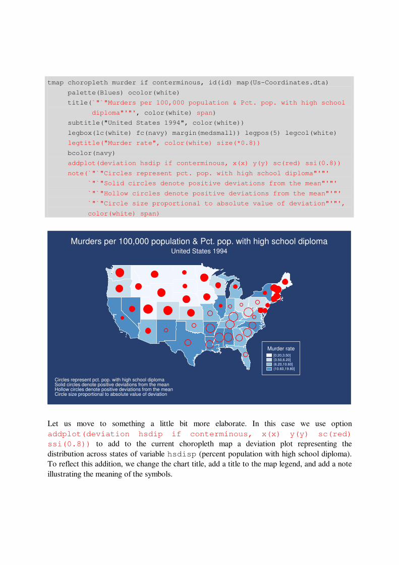
Let us move to something a little bit more elaborate. In this case we use option addplot(deviation hsdip if conterminous, x(x) y(y) sc(red) ssi(0.8)) to add to the current choropleth map a deviation plot representing the distribution across states of variable hsdisp (percent population with high school diploma). To reflect this addition, we change the chart title, add a title to the map legend, and add a note illustrating the meaning of the symbols.

tmap choropleth winner if conterminous, id(id) map(Us-Coordinates.dta)

clmethod(unique) palette(Custom) colors(`"`"203 24 29"'"' navy)

title(US Presidential Elections 2004) subtitle(% votes for Bush)

legpos(5) legsize(1.2) legtitle("Winner", size(*0.8)) legcount

addplot(label votebushpct if conterminous, x(x) y(y) lc(gs14) ls(0.9))

45.6 59.1

44.6

62.9

59.9

68.7

49.368.4 38.8

47.6

47.2 48.9

49.9 36.865.9

40.1

48.543.938.7

46.259.950.5 71.5

44.4

50.844.5

9.345.856.1 43.051.7

59.662.0

53.753.3

54.9

65.6 56.056.8

61.1

49.8

62.559.5 58.0

57.954.3

56.7

52.1

47.8

Bush (30)Kerry (19)

Winner

% votes for BushUS Presidential Elections 2004

Let us conclude our little tour with a map representing the results of the 2004 U.S. presidential elections. Here, we can note the use of the new option legcount to show – in the map legend – the number of states belonging to each class. 5 Acknowledgments The color schemes used in tmap choropleth were designed by Dr. Cynthia A. Brewer, Department of Geography, The Pennsylvania State University, University Park, Pennsylvania, USA. The color schemes are used with Dr. Brewer’s permission and are from the ColorBrewer map design tool available at ColorBrewer.org. I wish to thank an anonymous reviewer and Nick Cox for helping improve the first release of the tmap package. The second release owes much to ideas and suggestions by Vince Wiggins and Nick Cox. Any remaining errors are mine.

6 References Mitchell, M. N. 2004. A Visual Guide to Stata Graphics. College Station: Stata Press.

Pisati, M. 2004. Simple thematic mapping. Stata Journal 4(4): 361-378.

tmap 2.0 user's guide - fm 2.0 user’s guide maurizio pisati department of sociology and...

Documents