Title Binary Decision Diagrams and Their Applications for VLSICAD( Dissertation_全文 )

Author(s) Minato, Shin-ichi

Citation Kyoto University (京都大学)

Issue Date 1995-03-23

URL https://doi.org/10.11501/3080926

Right

Type Thesis or Dissertation

Textversion author

Kyoto University

Binary Decision Diagrams and Their i\pplications for VLSI CAD

Shin-ichi ~1inato

December 1994

Abstract

Manipulation of Boolean functions is a fundamental of comput("r science. Many problems in digital system design and testing can b(" cxpr<'ssed as a sequence of operations on Doolean functions. With th<' recent advance in very large­scale integratioll (VLSI) technology, the probl<'ms grow larg<' beyond the scope of manual design , and the computer-aided d<'sign (CA D) syst<'ms hav<' become widely used. The performances of these systems gn•at ly d<'J,<'nd on th<> <>fficiency of Boolean function manipulation. It is a very important technique not only in VLSI CAD systems but also in many problems of computer scicnc<', such as artificial intelligence and combinatorics.

A key to <'fficient Boolean function manipulation is to have• a good data struc­ture. Binary Dectsion Diagrams (BDDs} arc g raph repr<'sentat ions of Bool<'an functions. Th<' basic concept was introduced by Ak<'rs in I 978, and <'fficient ma­nipulation methods was developed by Bryant in 198(). Sine<' lh<'n, BDDs hav<' atl racted the attention of many researchers bccaus<' of t hc•ir good propel"t i<'s to represent Boolcan functions. A BOO gives a canonical form for a Bool<'an func­tion, so that we can easily check the equivalence of two functions. Although a BDD may become exponential size for the numlH'r of inputs in t h<' worst case, the size varies with the kind of functions , unlike truth t.ahl<' always r<'quir<' 2n bit of memory. It is known that many practical functions can he rC'pres<'nted by a feasible size of BDDs. This is an attractive feature· of BDDs.

This tlH•sis discusses the techniques related to BDDs and tlwir applications for VLSI CAD systems. In Chapter 2, we start with describing t !1<' basic concept of BOOs and Shared DOOs. We then prC'sent tlw algorithms of Boolean function manipulation using BOOs. In implementing f3DD manipulators on computers, the memory management is an important issuC' for tlw syst<'JII performance. \Ve show such implementation techniques to makC' f3DD manipulators applicable to practical problems. As an improvement of T3DDs, W<' propose the use of allributcd rdges, which are the edges attached with sc'\'C'ral sorts of attributC's reprcs<'nting a certain operation. Using these tN hniqtH'S, we implemented a BDD subroutine package for I3oolean function manipulation. It can cWcicntly represent and manipulate very large-scale T3DDs containing mor<• than million of nodes. Such Boolean functions have never h<'en dc•alt with by other classical methods. We show some experimental results to evaluate• th<' applicability of the BD 0 package to practical problems.

In Chapter 3, We discuss the variable ordering for J3J)I)s. It is important for

11

utilizing BDDs sine·p the siz<> of BDih grc·atly cle•pends on tile• order of t.lw input variables. lt is diffic:ult to derive· a nwt.hocl that always yic•lds t ll<' best ord<'l' to minimize BDDs, hut with some h~urist i<' nwthods, we can find il fairly good ordrr in many < <tsc·s. \Ve first consid<'r gc•twra I proper! ies on \'aria blc· ordcri ng for BD Ds. Basc·cl 011 t lw <'ousiderat ion, we· P~'<~!H>S<' t. wo hcu rist ic uwt hods of ,.aria ble ordcring. 011<' nwt hod, named dyTiamif' ll't ighl a~::.ignmwl m ethod, fi11ds a11 appropriate• ord<'r bc.for<' gcnNatillg the· BDD. It refers topological i11formation oft he Boolc·an c·xprc.-.;sion or logic circuit which specifics the• sc•qu<'IH'<' of BDD ope·rations. Tl1<: othe·r method, nanwd mi11imum-width method, rc·duccs BDD size by rcordc•riug the· input variables for a given BDD with a c<>rtain initial order. We implc•nwntcd the two met hods and conducted SOI11<' <'Xpcrimcnts. Experimental rC'sults shows that our met hods arc• effective to r<'ducc BDD si!.<' in many cases, and useful for practical applications.

In Chapter '1, \\'e discuss the r<'prc•sentation of multi-valuc:cl functions. In many problems 111 digital system dPsign. wt• sometimes use ternary valued func­tions containing don't cart-s. There are t\\·o methods to extend BDDs to deal with tcrnary logic~; ltr1UH'Y-I'alucd IJ[)/) . .., and using a pair of/]/)/),., \\'e com pare and clarify t he• rc•lationship of t he• two methods by introducing a special input variable>, ntll<'d D-t•m·iablc. In this discussion, we show that the difference oft he two mc:t hod Utll be concluded into vnriahle ordering. This argutncnt is cx­lcndcd into 11 ary valued functions. Some• vari.Ult of BDDs have been de\ iscd to

represent multi-vahwd functions. \\'t• sun·cy these methods and compare them as well as on t ht: t t:rnary-valued fun et ions.

Om• oth<'r topic is how efficiently lransfonn BDD rcpresc:ntatiotl into other d<\ta struclttr<'s. Chapter 5 presents a fast met hod for generating prinw-irredundant forms of cube s<'l.s from given BDlh Prime-irredundant means" form such that each cube is <t prime• implicant and no cuhe can be climinatc·cl. Om algorithm g<·ncrates con1pad rulH' :;et:; directly from BD Ds, in contrast lot hC' conventional cube set rcduct ion algorithms, which contmonly manipulate redundant cube sc•ts or truth tables. Our method is bas<•d on the idea of a rccur.~u·£ opcmlor, pro­posed by \lorn•ale. \ 1orrcale's algorithm is also hascd on cube sc•lmanipulation. \\'e found t bat t h<" algorithm can he imJHO\·cd and rearranged to fit BDD op­c:rations effkic•nt.ly. The experimental n•stdts demonstrate that om method is <'frkicnt in l<'rms of time and space. In practical time, we can gc'nNatc cube sets conc;isting of mort' than 1,000,000 litc•rals from multi-level logic rirruits which have ncv<'r pr<'viously l><'en flatt<'n<'d into two lcvc·l logics. Our mclhod is morP t.ban 10 ttm<'s faster than rom·<'ntionalmethods in larg<>-scalc• exatnplc•s. It gives quasi-minimumtntmhcrs of cub<'s and lit<'l'als . rhis method will find many useful applications in logic d<':-;ign systems.

.\sour understanding of BDDs has ci<'CJH'ned, the range of applications has broadened. BC'..;iclt•s Boo lean functions, we a re oft en faced with manipulating , ... (/ _.., of combinations to d<•al with many problt•ms, not only in tlw digitc1l syst <'Ill design hut also various an·as in computer scit'IKt'. B) mapping a s<'t of combinations into the Boolean span', it can be rc•pn·sc•nlt'd as a characteri:-,tir f11nction using a BDD. T his met hod enables us to manipulate· a hug<' numlH'r of combinations

Ill

implicitly. which has ne,·c·r lwcn practical hdore. lloW<'\W, this BDD ha~wd set r<'prcsentation does not cotnpl<'lc>ly match tht• prO!H'rties of BDDs, th<'rcforc sonwt inws the size of BDDs grow large hecaus<' the rcduct ion rules arc• not cffc•ct ivc•. 'l'h<'re is room to intpron• the data st ruct tlrt' for l'<'j>rt•scnt ing sds of comhinat ions.

In Chapter 6. we propo.,<' Xcm-~11ppt't'·'t'd IJ/)1)., j O-~up-U[)JJ.,), which <Ht'

BDDs has<'d on a rww reduction rule•. I his data structmc h ctdapted to n•pn•st•nt ,..;( t., of rombination::.. 0-sup-BDDs can manipulate S<'b of combinations 111on• c•lfi . cicnt I) than using convc·nt ional BD Do.;. \\'e discuss t 11<' properties of 0 sup-BDDs and their <'fficiency basc•d on a statistical expc•rinwnt. \\c• thc·n pr<'SC'nt t IH· basic op<•rators for 0-sup-BDDs. Those• opc•rators are dc·fitu•d as the> operations on st•ts of combinations, which slightly differ from t h<' Boolean function manipulation has<'d on conventional B)) I h .

Wlwn describing algorithms or procedures for manipulating BDDs. we· usu­ally us<' Boolean expressions hascd on switching algc•hra. ~imilarly. wh<'n consid­ering s<'fs of combinations with 0-sup BDDs. we can use· 1111a/c cubt stl e:qn<'S· sions and thC'ir algebra. Bas<•d on unatc cube sd algebra, we• can simply dc·scriiH' algorithms or procedurc•s for 0 sup-BDDs. \\'e dcvclopt•d efficient algorit lttns for c·xc•cuting unatc> cube sd opc•rcll ions including 11111lt tplicat ion and division. l lc·n· we• discuss calculation of unate• cube set algebra using 0-sup BDDs \Vc• propose• eflicic•nt algorithms for computing unate cuiH' sd op<'r<d ions. and show sotllt' practical applications.

In Chapter 7, an application for \'LSI logic ~yntlu:sis is presentc·d We• pro­pose a fast factorization mc•t hod for cube set rcpH'sc•nt at ion represc·ntcd with 0-sup-BDDs. Our new algorithm can be executed in a time almost proportional to tlw size of 0-sup-BDDs. which arc usually rnurh -.;maller than tiH' numlH'r of lit<'l'als in the cube set. By using this method, we· can quickly generate mult.i kwl logics from implicit cube sets evc•n for parity functions and full-addc•rs, which have ll<'W~r been pos~ihlc• with the conventional nwthods. We implemc•nt<'d a JH'W multi -lcvcllogic synt he~izrr, and cxp<'rirnc•ntal rc•sults tndicatc our met hod is much fast er than con H•nt ion a I rnc>t hods and clt ffcrC'ncc:s are m or~ sign i fie ant for larg<•r-scalc problems. Our nwt hod grcatly accelerates multi -lcvcllogic syntll<'sis systems and enlarges t lw scale of applicable circuits.

In Chapter 8, we presents a helpful tool for the research on computer scie•11n!. \ \ ' hen we are considering prohl<'ms re! a !.<'d to logics, we• sonwti rn<'s fa c<'d with t lw task lo describe and calcul;ttc• Boolc-an expressions. Jt is a curnlwrsonlC' job to calculat<• or r<'ducc Bool<•an c•xpressions by hand. so we• clc·v<'IOp<'d a compute·r aided Boolcan expression maniplllator. Our prod tu t, caiiC'd RE\1-11. feat urcs that it calculates not only binary logic operation hut also anthm<'tic op<'I'Htions on multi-\·alued logics. such as addition. subtraction. multiplication, division. equality and inequality. Such arit lnnctic operati<ms proviclc· simple cl<-!-i<:ript ions for various problems. B E~l- [I fc·c•ds and compu t c·s the: problems n·pn:sc·nt eel by a ~wt of equalities and in<'qualit ies. which are clc-alt with using 0-1 lin<'<ll programming. \\'e discuss th<: data stmcture and algmithms for the arithnwtic operations. Finally we pn·s('llt the ~·qwcification of BEi\.1 11 and somC' application

lV

examples, such as the 8-Queens problem. Experimental results indicate that it has a good computation performance in terms of the total time for programming and execution.

Conte nts

Abstract

1 I ntroduction 1.1 Background . . . . . 1.2 Outline of the Thesis

2 Techniques of BDD Manipulation 2.1 Introduction .... .

2.1.1 BDDs .......... . 2.1.2 Shared BDDs ..... . .

2.2 Algorithms for Logic Operations . 2.2.1 Data Structure ... . 2.2.2 Algorithms ..... . 2.2.3 Memory Management.

2.3 Attributed Edges ... 2.3.1 Negative edges . 2.3.2 Input Inverters . 2.3.3 Variable Shifters 2.3.4 General Consideration

2.4 Implementation and Experiments 2.4.1 BDD Package ..... 2.4.2 Experim<'ntal Results

2.5 R<'marks and Discussions ..

3 Variable Orde ring for BDDs 3.1 Introduction ............. . 3.2 Properties on th<' Variable OrdNing . 3.3 Dynamic Weight Assignment \1d hod

3.3.1 Algorithm ...... . 3.3.2 Experim<'ntal Results .

3.4 Minimum-Width M<'thod .. 3A.l The Width of BDDs . 3.4 .2 Algorithm ...... . 3.4.3 Experim<>ntal Results .

3.5 Conclusion . . . . . . . . . .

V

1 1 3

7 7 7 9

9 11

11

14 15

15

17 17 18 19

19 20 21

23 23 21 2G 26 27 28 28 30 31 33

\'I

4 Representation of Multi-Valued Functions tJ .1 H<•Jm•sentat ion of Don't Care ...... .

-1.1.1 Bool<·an }·unctions with Don't Care 1.1.2 Ternary-Valued BD J)~ and BD)) Pairs L I.:J D-variable . . . . . . . . . . . . ...

1.2 Hq>r<'S<'ntat ion of Bool<·arr to-IntegC'r Functions 1.:3 H<·marks and Discussions ..... . ..... .

5 Generation of Cube Sets from BDDs 5.1 Introduction ............. . 5.2 Conv<'ntional t-.1cthods ....... .

5A

C:c·rH•ration of Prime-Irn•dundant Co\'C·rs 5:3 I Prilll<'· ln<'dundant Cube SC'ts . . .).:J.2 ~1orr<·<dc\; Algorithm ...... . s.:L:l ISOP Algorithm Based on BDDs !) :lA Techniqu<'s for lmplc•mcntation Lxp<'rirnental Hcsults . . . .... S.-1.1 Comparison \\'ith ESPRESSO !l.-1.2 Effect of Variable Ordering . !>.1.:3 Statistical Propc•rt i<•s

5.5 Cone Ius ion . . . . ..

6 Zero-Su ppressed BDDs 6.1 lnt roduction ........... . 6.2 BDDs for Sets of Combinations .

G.2.l Rcduct ion Rules of BDDs G.2.2 Sets of Combinations .

6.3 Z<•ro-Suppr<.•ssed BOOs .... 6.4 .\1anipulation of 0-Sup-BDDs

6.1.1 Basic Operations 6.-1.2 Algorithms 6.1.:3 Attributed EdgC's

6.S U nate Cu bP S<'t Algebra 6 !l. I Basic OpC'rations 6.5.2 Algorithms

6.6 Implementation and Applications 6.(i.l 8-Qu<'<'ns Problem 6.6 2 Fault ~imulation

6.7 Conclusion ........ .

7 Multi-Level Logic Synthesis Using 0-Sup-BDDs 7.1 Introduction. . .......... . 7.2 Implicit Cube• Set Representation ....... .

7.2.1 Cub<' Sd ReprC's<•ntation l'sing 0 Sup-BDDs 7.2.2 ISOP Algorithm Balied on 0 Sup-BOOs ...

C'O.V'l'E.\'TS

35 3!) :n :36 37 38 11

43 1:3 -1-1

·15 4;)

·16 47 ·18 19 19 50 51 .')2

55 5.)

55 .)6 57 58 60 60 61 63 64 64 66 68 69 70 71

73 73 74 1·1 7.5

COXTESTS

7.3 Factorization of Implicit Cub<' S<'t Hcprc~cntation ..... . 7.:3.1 Weak Division ~lethod ................ . 7.:3.2 Fast \\'eak-Divisron ,\lgorithrn Based on 0 Sup 13DDs 7.:3.3 Divisor Extraction

7.4 lmpkmentat ion and Exp<•rimcntal H<•strlts

7.5 Conclusion ................. .

8 Arithmetic Boolean Expressions 8.1 Introduction . . . . . . . . . . . . ... . 8.2 Manipulation of Arithnwt ic Bool<'an Exprc>ssions .

8.2.1 Definitions ............. . 8.2.2 Reprcsmtation of B to-I Functions . 8.2.3 Handling 13 to 1 fun< tions . . ... . 8.2.4 Display Formats for 13 to-1 Functions

8.3 Applications ................ . 8.3.1 BEM II Specification ........ . 8.:3.2 Timing Analysis for Logic Circuits . 8.:3.3 SchC'dulrng Problem in Data Path Synthesis 8.:3.4 Other Combinatorial Probl<'ms

8.4 Conclusion .

9 Conclusions

Bibliography

Acknowledgment

List of Publications by the Author

\' 11

11

77 79 80 81

82

85 85 86 8G 87 8!) !)0

92

n 91 !)6

97 !.)8

99

103

109

111

Vlll CONTENTS

Chapter 1

Introduction

1.1 Background

Manipulation of Boolean functions is a fundamental of computer science. Many problems in digital system design and testing can be expressed as a sequence of operations on Boolean functions. With the recent advance in very large­scale integration (VLSI) technology, the problems grow large beyond the scope of manual design, and the computer-aided design (CAD) systems have become widely used. The performances of these systems greatly depend on the efficiency of Boolean function manipulation. It is a very important technique not only in VLSI CAD systems but also in many problems of computer science, such as artificial intelligence and combinatorics.

A key to efficient Boolean function manipulation is to have a good dala structure. It is required to perform lhe following basic tasks efficiently in terms of execution time and memory space.

• Generating a Boolean function data which is the result of a logic operation, such as AND, OR, NOT, and EXOR, for given Boolean functions.

• Checking tautology or satisfiability of a given Boolean function.

• Finding an assignment of input variables such that a given Boolean func­tion become 1, or counting the number of such assignments.

Various methods have been developed for representing and manipulating Boolean functions. There are several classical methods, such as truth tables, pa1·se t1·ees and cube sets.

Truth tables are suitable for manipulating on computers, especially on recent high-speed vector processors[IYY87] or parallel machines. However, they need 2n bits of the memory to represent ann-input function, even for very simple func­tions. For example, a lOO-input tautology function requires a 2100 bit of truth table. Since exponential memory requirement leads to an exponential computa­tion time, truth tables are impractical for manipulating Boolean functions with many input variables.

2 CHAPTER 1. ISTRODLTCTIOS

Par.-;c trees for Boolean expressions sometimf's give compact representations for the functions with many input variables, which cannot be represented com­pactly using truth tables. However, there exist many different expressions for a giv<'n function. The equivalence checking of the two expressions is w·ry hard as it is an NP problem, although thC're have been developed the method of rule-based transformation of the 8oolf'an exprcssions[LC'~189].

C1lbc scls (also called sum-of-products, PLA forms, cover:;, or two-level logics) are regarded as a special form of the Boolean expressions with the AND-OR two level structure. They have bcf'n extensively studied for many years and employed lo represent Boolean function on computers. Cube sets sometimes giv<' more compact representation than truth tables; however, redundant cubes may appear in logic operations, so they have to be reduced to check tautology or equivalency. This rc>duction process is time consuming. There are other drawbacks that NOT op£>ration cannot be performed easily, and that parity functions become exponential sizes.

Unfortunately, the above methods are impractical for large scale problems be­cause of their drawbacks. An efficient method for representing practical Boolean fund ions have heen d<'sired.

Binary Dcci.'lion Diagrams (BDDs) are graph representations of Boolcan functions. The basic concept was introduced by Akers in 1978[Ake78], and efficient manipulation methods was developed by Bryant in 1986[Bry86]. Since th<'n, nODs have attracted the attention of many researchers because of their good prop<'rties to represent Boolean functions. A BOO gives a canonical form for a Uoolean function, so that we can easily check the equivalence of two func­tions. Although a BOO may become exponential size for the number of inputs in the worst case, the size varies with the kind of functions, unlike truth table always require 2n bit of memory. It is known that many practical functions can be reprr~enkd by a fcasiblf' size of BDDs. This is an attractive feature of BOOs.

ThNe have been a number of attempts to improve the BDO technique in terms of execution time and memory space. One of them is the technique of shared BDDs (SBDDs)[MIY90], or multi-rooted BOOs, which manage a set of BDDs by joining them into a single graph. This method reduces memory re­quirC'mcnt and makes easy to check the equivalence of two BODs. Another improvement of BOOs is the negative edges, or typed edges[MB88] They are attributed edges such that each <'dge has an information of inverting. They are effective to reduce the operation time and the size of the graph.

Using BODs with those improvement methods, Boolean function manipu­lators are implemented on workstations and now widely distributed as BOO packages[Min90]. They have been tried to utilize in various applications, es­pecially in the VLSl CAD systems, such as formal verification[FFI<88, MB88, HCl\1090], logic synthesis[CMF93, MSB93], and testing[CHJ+9o, TIY9l].

BDDs have exce!lent properties to manipulate Boolean functions; however, there are som<' problems to be considered when utilizing BOOs to practical applications. One of the problems is variablf> ordering. Conventional BOOs requires to fix the order of input. variables, and the size of BOOs greatly depends

1.2. OUTLINE OF THE TllESJS 3

on the order. It is hard to find the best order which minimize BOOs. Variabl<' ordering algorithm is one of the most important issues for utilizing BDDs. As another problem, we sometimes manipulate ternary valued functions containing don't care to mask unnecessary information. ln such cases, we have to devise a way of representing don't cares since usual BOOs deals with only binary logics. This issue can be generalized into the method of manipulating multi-valued logics or integer functions using BOOs. One other topic is how efficiently transform BDD representation into other data structures, such as cube sets, or Boolean expressions. This method is important in practical applications to output the result of BDD manipulation.

As our understanding of BDDs has deepened, the range of applications has broadened. Besides Boolean functions, we are often faced with manipulating sets of combinations in many problems. One proposal is for multiple fault sim­ulation by representing sets of fault combinations with BDDs[TlY91]. Two others are verification of sequential machines using BOO representation for state sets[BCM090], and computation of prime implicants using Met a P1'oducts[CMF93], which represent cube sets using BOOs. There is also general method for solving binate covering problems using BODs[LS90]. By mapping a set of combinations into the Boolean space, it can be represented as a characteristic function using a BOO. This method enables us to manipu late a huge number of combinations implicitly, which has never been practical before. However, this BDD-bascd set representation does not completely match the properties of BD Os, therefore sometimes the size of BDDs grow large because the reduction rules arc not ef­fective. There is room to improve the data structure for representing sets of combinations.

1.2 Outline of the Thesis

This thesis discusses the techniques related to BOOs and their applications for VLSI CAD systems. Chapter 2 to 5 discuss implementation and utility tech­niques of BDDs. Chapter 6 and 7 propose zero-suppressed BDDs, which is a vari­ant of BDO adapted for representing sets of combinations. Chapter 8 presents an arithmetic Boolean expression manipulator, which is a helpful tool to the research on computer science.

In Chapter 2, we start with describing the basic concept of BD Os and Shared BOOs. We then present the algorithms of Boolean function manipulatio11 us­ing BOOs. In implementing BOO manipulators on computers, the memory management is an important issue for the system performance. We show such implementation techniques to make BDD manipulators applicable to practical problems. As an improvement of BOOs, we propose the use of attributed edges, which are the edges attached with several sorts of attributes representing a cer­tain operation. They are regarded as a generalization of the inve?'ter{Ake78], or typed edges[MB88]. Using these techniques, we implemented a BOD subrou­tine package for Boolean function manipulation. It can efficiently represent and

4 CHAPTER 1. /1\'TROD c.; eT ION

manipulate vC>ry larg<'-scalc BDDs containing more than million of nodes. Such Boolean functions haw never been dc·illt with by other classical methods. We show some experimental results to C>valuate the applicability of the• BDD package to practical proble•rns.

In Chapte•r :~. We· discuss the. variable ordering for BOOs. It is important for utilizing BDDs since the size of BDDs gn·atly depends on the order of the input variablcs[FI·I\88]. It is difficult to derive a method that always yields the best ordC>r to minimize BDDs, but with some IIC'nristic methods, we can find a fairly good ordPr in many cases. \Ve first consider general pro pert i<'s on variable or­dering for BDDs. Bas<'d on the conside•ratron, we propose two heuristic methods of variable· ord<'ring. Onc> method, named dynamic wezght ass1911menl method, finds an appropri<ttc ordN before gerH'I'<tting the 13DD. It refers topological in­formation of th<' Boolcan expression or logic; circuit which specifl<'s the sequence of BDD operations. I'h<' other method, named minimum-width m c./hod, reduces BDD sizt· by rt'<Hd<•ring the input ,·ariahlcs for a given BDD with a certain ini­tial ord<'r. Wt• impl<'nwnted the t \\'O nwt hods and conducted som<' <'xperiments. Experimc·ntal n·sults shows that our methods are effective to reduce' 1300 size in many cases, and useful for practical applications.

In Chapter 4, We• discuss the repre•s<·nt at ion of multi -vahH•d logic functions. In many problems in digital system dc•sign, we sometimes use ternary-valued functions containing don't cares. There are two methods to extend f3DDs to d<'al with tt'rnary-valut'd logics; IU'nary-1•aluu/ IJDD3 and using IJ[)[) JHw·s. \\'e compare and clarify th<' relation~hip oft he> two methods by introducing a special input variable·, C<tllcd D-t•ariablc. In this discussion. we show th<tt tit<' difference of the two nwthod C<Hl be concludt•d into variable ordering. This argument is c•xtendcd into multi valued logic functions which dt•al with intc•g<'r values. Some variants of Bf)l)s havc> been dPvis<'Cl to represent multi -valtwd logic func­tions, such as mul/1 lcnnmal 13[)1) .... (AIT/3DDs}[RFG+93] and using BDD neciors which we proposc•d[Min9:3a]. \\'c dc:-.nilw tlws<' methods and compare them as well as on tlw tc•rnar.\' valued fund ions.

Chapkr f) pn•sc•nts a fa:-;t mc•thod for g<'ncrat.ing primc-irre•dundant forms of cuhc s<'ts from gi\'cn BOO:;. Prinw-irre•dundant means a form such that each cube is a prinw irnplicant and no nrhc> can be climinatt•cl. Our algorithm g<'ll<'ratC's comJ>CH't ruhc sets directly from BD Ds, in contrast tot he con,·cnt ion a I cuh<' ~et r<'durtron algorithms, \\'hich rotntnonly manipulal<' n•dund<wt cube s<>ts or lrulh tahlc•s. Our md hod is based on I Ire• idea of a 1'frurstl'<' opr mlor, proposed hy ~lorrcalc·. Morrcale's algorithm is also has<'d on cube set manipulation. \V(' found that I h<' algorithm can h<' improvc•d and rearranged to fit BDD op~rat ions l'lliciently. Tht• <'Xp<'rinwntalrc:mlts dt•rnonst rate that our nwt hod is t•flicicnt in tc•rms of time and span·. In practical t inw. wc• can gcncratl' ruht• sc·ls consisting of more than 1,1100,0011 lit1•ral..; from nutlti -It•n·l logic circuit:-- which Iran• never pn·,·iously be<'n llatte•tu•d into two lt·wl logics. Our nwthod is mor<' than 10 times faster t h<\11 FSJ)H /:'SSO[BII \1<-i\ "t] in large-scale examplt•s. It gi,·es quasi­minimum numiH'rs of cubes and lil<'rals. This mdhod will find many useful applications in logir d<'sign syst<•ms.

1.2. OUTLINE OF THE TIIESIS 5

[n C'hapter 6, we propose Zero-Suppressed HD/Js (O-Sup-BDD5), which ar<' BOOs based on a new reduction rule. This data struct ttr<' is adapted to srls of combinations, which appc•ar in many combinatorial problems. 0 sup BDDs can manipulate sets of combinations more efficiently than using conventional BDDs. We discuss the properties of 0-sup-BDDs and their efficiency baS<.•d on a statistical experiment. We then present the basic operators for 0 sup BDDs. Those operators are defined as the operations on sds of combinations, which slightly differ from the Bool<'an function manipulation hased on conv<·nt ional BDDs.

Wh<'n describing algorithms or procedures for manipulating BDDs, we usu­ally use Boolean expressions basc•d on switching algebra . Similarly, when consid­ering s<'ts of combinations with 0 sup BDDs, we• can use• unalc cub( ,.,(f <'xpr<'s ­sions and their algebra. Bas<'d on unale cube· sd algebra, we• can simply cl<•sc riiH' algorithms or procedures for 0-sup.BDDs. \\'c dcvelopc•d t•Hiri<>nt algorithms for executing unate cube set opcrat ions including multiplication and di\ ision. llt>rc· we discuss calculation of unal<' cull<' sd algebra using 0-sup BD Os. \\'<' JHOJH>st• effici<'nt algorithms for computing unat<> cube s<'t OJH'ratrons, and show sottH' practical applications.

Jn Chapt<'r 7, an application for \'LSI logic syntlu·sis is JH<'s<'nl<•d. v\'<• pro pose a fast factorization nwthod for cubf! s<'t r<'prc•st•ntation n·prescntc·d with 0-sup-BDDs. Our n<'w algorithm can bc <>X<'Cllt<'d in a t inw almost proporl ion a I to th<' size of 0-sup-BDih, which arC' usually much smaller than th(' numlH'r of literals in the cube set. By using this nwt hod, '''C can quickly generate multi-l<•vc•l logics from implicit cube sets <'\'<'11 for parity fun et ions and full addc·rs. which hav<' n<'V<'r hcen possiblc> wtt h the conventional nwt hods. \Vc· implc•nwtrlc•d " n<'w mult i-levc>l logic synt lwsizN, and expcrim<'ntal n•stdts mdicatc our 111C'I hod is much faster than conv<'ntionalllldhods and diffcrc•ncc•s <1 re• more signifin111t for larger se ill<• problems. Our md hod grc·at.ly arcel<'ralcs 1111rlt i lc·vd logi<' synt lw~is

systems and cnlargc>s the scale• of applicable circuits. In Chapter 8. we presents a h<'lpful tool fort lw H's<·arTh on <·ompulc'r sl'i< ·nc·c·.

\\'hen we are considering prohlc•nJs rc>latc•d to logic:; , W<' sottwl inws facl'd wit lr till' ta.o;k to de•scribe and calculate• Boolcan <'Xpr('ssions. lt i:-; a nJnJlwrsonH' job to cakulat<' or reduce £3ool<'an c•xprc·ssions by hand, so we· d<'\'c•lopNl a cotllJHitt ' l'­aidcd Boolcan expression manipulator. Our product, call('(! /Jrh\1-11, fc·at lll<'s that it calnt!atf's not only bin My logi( opcration but. also <ttitltnwtH <>Jwrat ions on muiLi-valuc>d logics, such ns ilddition, subtract ion, tnult iplication, drvision, equality and inequality. Such arit hmf't ic opcrat ions provide' simpl(' dc>script ions for various problems. BE~l- 11 fc~·ds and comput< 'S tlw pHJIJlc·ms r<'JHC!:-i<'IJicd hy a sd of cqualities and iJwqualit ic·:-.. which aw d<•alt wit lr using 0-1 litwat programming. \\'e discuss tlw data structmc• and <tlgoritltms for tlw aritltnwtic operations. Finally\\'<' prc•s<·nt t he• SJwc·ifiraticm of HE.\1-11 and some· application example•s. such as the ti-Qrw<:JIS problc•Jn. Expc:rinwntal rc·.sults indicate: that it has a good computation J>C'rfonnilnre in terms oft lw total t inw for program111ing and <'X<'Cttt ion.

In Chapl<'r 9, the conclusion of this th<'<>is nnd future• works arr statc•d.

6 CHAPTER 1. INTRODUCT/0.\'

Chapter 2

Techniques of BDD Manipulation

2 .1 Introduction

This section introduces basic definition of BDDs and shared BDDs which will be discussed in this thesis.

2 .1.1 BDDs

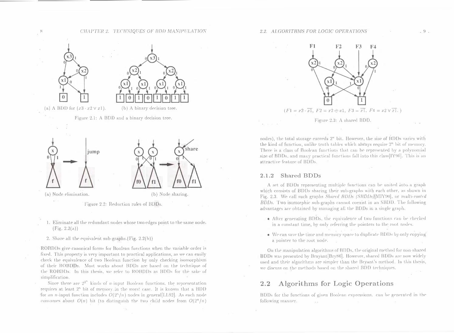
BDDs are graph representation of Boolean functions, as shown Fig. 2.l(a). The basic concept was introduced by Akers[Ake78], and an efficient manipulation method was developed by Bryant[Bry86].

A BDD is a directed acyclic graph with two terminal nodes, which we call the 0-terminal node and 1-terminal node. Every non-terminal node has an index to identify an input variable of the Boolean function, and has two outgoing edg<'s, called the 0-edge and l-edge.

An Ordered BDD (OBDD) is a BDD such that the input variables appear in a fixed order in all the paths of the graph, and that no variable appears more than once in a path. In this thesis, we use natural number 1, 2, ... for the indexes of the input variables, and every non-terminal node has a greater index than its descendant nodes.

A compact OBDD is derived by reducing a binary tree graph, as shown in Fig. 2.l(b). In the binary tree, 0-terminals and !-terminals represent logic values ( 0/1), and each node represents the Shannon's expansion of the Boo lean function:

f = Xi · fo V Xi · f1 ,

where i is the index of the node. fo and f 1 are the functions of the nodes pointed by 0- and l-edges, respectively.

The following reduction rules give a Reduced Ordered BDD (ROB DD).

7

8 Cll1\PTER 2 '1 EC'I!NIQUES OF BDD MANIPULATI ON

(a) A BDO for (.r:l J·2 V xl ). (b) A binary decision tree.

Figure 2.1: A 13D D and a binary decision tree.

jump

(a) Node elimination. (b) Node shari11g.

Figure 2.2: Hcduction rules of BDDs.

1. Eliminate all the redundant nodes whose two edges point to the same node. (Fig. 2.2( a))

'2. Share a ll th<' equivalent suh-graphs.(Fig. 2.2(b))

RO BDDs give canonical forms for Boolean functions when the variable order is llxc•d. This property is very impotl ant to practical applications, as we can easily dwck the equivalence of two Boolean function by only checking isomorphism of thei r 110BDDs. t-. lost works about BDDs are based on tlw tc•chnique of the HO BDDs. l11 this thesis. W<' rc•fC'r to ROBDDs as BOOs for t lw sake of si mpli heat ion.

~tnn' there an• 2l" kinds of n-input BooiC'<ln functions. tlu· r<'J>t<'sentation requires at least :2" bit of rnemor~ in the worst cas<'. lt is known that a BDD for an 11 input funcl ion includes 0(2" jn) nodes in gc•ncral[LL92]. As each node consumes about O(n) hit (to distinguish tlw two chi ld nodes from 0(2n jn)

2.2. ALGORIT HMS FOR l-OGI C OPEHATIONS

Fl F2 F3 F4

(Fl = x2 · XT, F2 = x2 6 :.rl. F:3 = xl, F4. = .r.2 V xl. )

Figure 2.3: A shared BDD.

9

nodes), the· total storage cxcccds zn bit. llowcvcr, the size• of BOOs \iHi<'s \.vith the kind of function. unlike• truth tabl<'s which always n•cptin· 2" bit of tnc•utory. There is a class of BooiC'an functions that can be n·pn·sc·u!C'd by a polyno111ial size of BDDs, and man) practical functious fall into I his class[IY90]. Tit is is an attractive feature of BDDs.

2 .1.2 Shared BDDs

A set of BDOs repr<'scnting multipl<• functions can lw unitf'd into a graph which consists of BDDs sharing their sub graphs with <'ach other, as shown iu Fig. 2.3. WC' call such graphs Sharul !300s (SBD/Js}[f\t iY90J, or nwllt roolul BDDs. T wo isomorphic sub-graphs c·aitllot. cocxisl in an SBDD. The following advantagc•s arc obtain<'d by managing all I hc BDDs in a s111gl<• graph.

• Aftc•r g<'ncrating BDDs, the cquiv<~lc•uce of two fun et icms ca11 lw checked in a constant time, by only ref<'ning the poi11t<'l's to th<' root nod<'s.

• We• can save the tirnc• and nwrnory space' to duplicate BDDs by only copying a pointer to th<' root node.

On the rn<~nipulatioll algorithms of BDDs. the original nwt.hod for non-shared BDDs was presented by lhayant(BryH6j. However, shan·d BDDs a rc now widc·ly used and thcir algorithms arc simpl(•r t.ltnn t.hc Bryant's Jll('tltod. In this t.ltc•s is, we discuss on the nwthods based on th<' sltarc•d BDD tc•dtniquc•s.

2.2 Algorithms for Logic Operations

BDDs for the• functions of givcn Boolc•<ut c·xprC'ssions. can IH' gencratc·d 111 t.he following ma11ncr.

10 CHAPTER 2. TECIIXIQUES OF BDD "\IASIPULATI0.\1

xl xl x2

Figur<' 2.4: Generation of BDDs for F = (xl · x2 V x3).

(address) No Nt N2 N3 N4 Ns N6

(index) (0-cdgc) (l-edge) - - -

- -Xt No .v. It Nt No X2 No N3 X2 N2 N3 X2 N3 NI

+-- 0 +-- 1

+-- F3(= xt) +-- Ft (= X2. Xi) +-- F2( = X2 EEl xl) t- F4( = X2 V I t )

Figure 2.5: BDD representation us ing a table.

1. Define a fixed order of input variables.

2. Make a BDD with a single node for each input variable.

3. Construct more complicated BOOs by applying logic operations on BDDs according to the Boolean expressions.

An example for F = (.r 1 • x2 V .r3 ) is shown in Fig. 2.4. First. trivial BDDs for Xt, x2 , x3 arc generated. Then applying the AND operation between l· 1 and x2 ,

the BDD of I 1 · .:r2 is generated. The final BDD for the entire expression F is obtained as the result of the OR operation between x 1 • x 2 and .r3 .

In this section we show the algorithms of logic operations on BODs .

2.2. A.LGORITII.\15 FOU LOGIC OPERAT/0.\S 1 I

2.2.1 Data Structure

In a typical implementation of the BDD manipulator, all the nodes arc stor<'d in a stnglc table on the main llH'Tllory of thc comput<•r. Each node has t hn·<· basic att rihutcs; an index of t lw input variablt• and two point<'rs of 0- and l ­edges. Some additional pointt•rs and counters an' at t acllt'd to the node data for maintaining the table. Figurt• 2.3 shows an examplt> of the• table rcpr<'st•nting BDDs shown in Fig. 2.3. 0- and 1-terminal nodes <H<' at first allocated in t.he tahlt• as the sp<'cial nodes. By reft•ning the address of a node>, we can imnH•diatt>ly know whether th<' nod<' is a t<'rminal or not.

In a shared I3DD, isomorphic sub-graphs should he• shar<•d without fail. :\anwly, Two equiYalent nodt•s n<'V<'r coexist. The propcrt~· is maintained by recording all the nocl<-s in a hash tabl<'. E\'t•ry time· wc• cht'ck the hash tablt· before cn·at ing a new nodt• . If I 111'1'<' alr<'ody t•xists a nodc• whost• conc•-;ponding

ind<'x , 0-cdge. and 1-cdg<' '" t' idt•n I ica I. we do not nc·a k a 11<'\\' uod<' but :-imply copy I he• pointc·r to the cxi~t ing nodt•. This task can ht> done in a constaut t illlt' if the• hash table acts succf'ssfully. Tht• pt>rformancc of tilt' hash table is important sinn· it is frequently referred iu the· BDD manipulation.

Using this techniqtu', a Boole•an function on a BDD rnanipulal01 can bt' ide·nt ified by the addr<'ss of t 11<' root node of th<' 131)1) C'ons<'quent.l), we• c.tn perform t he• cqui\'al(>ncc dwcking or tautology ciH•cking of Boolc•an funct io11s by only comparing the addn•ss<'s of tll<' root nodes of the• BDDs mdcpc•ndc·nt of tlw numb<'r of nodes.

2.2.2 Algorithms

Binary Logic Operations

The binary logic operation is t.h<' most important part i11 the techniques of BDD manipulatiOn. Here we show the algorithm of gerl<'ratmg a BD D which n•prc•sc•nt.s

the result of a binary operation Jog. for given two BDDs of J and g. This algorithm is based on the following formula:

Jog = v. Ucv=O) o g{v::O)) V l' . (f( v=l) o 9<• : I}),

This formula means that the• op<'ration can be c•xpa11d<'d to two sub-or)('rations

(f{t•=O) o.%• oj)) and Ucv- t) og(u- t)) with respect to an input variable v. lle' l><'<ll ing the expansion recursivdy for each sub-operation by all the input variahlf's, they are eventually broken down into trivial ones and the results arc obtaitH•el.

The algorithm of computing h (=Jog) is summarizc•d as follows. Ilere J.top denotes the input variable oft he root node of f. fo and [ 1 arc the BOOs pointc·d

by 0-cdge and l-edge from the root node. respc•ctive•ly.

I. When J or g is a con<;tant, or the case of J = g: return a result according lo the kind of tlw OIH'rat ion. (Example) J · 0 0, f V f f. f 4 1 = 1

12 CHAPTER 2. TECII.\'IQL'ES Of' BDD .\1ANIPULATIOS

••• OP· •• .. .. r ... ··. g

/(/)·(5)~ (3)-{5) {2)·{5)

/ \ / " (3)-(7) (3)·(6) (3)-(7) (4)-(6)

1\ 1\ I\ I\ (4)·(7) (4)·(8) (4)-(7) (4)-(7) (4)·(8) !\ 1\ !\/\ /\

(a) An example. (b) Strucl urc of procedure calls.

Figure 2.6: Procedure of binar.> operation.

2. If f.top and g.top are identical: ho .__ fo o go; h 1 .__ !1 o g1; if (h 0 - h.) h .__ h0 ;

else h .__ Node(J.top, h0 , ht);

:l. If f.top is higher than g.top: ho .__ fo og; ht .__ ft og; if ( h 0 = h.) h - ho; <'is<' h - Node(f.lop, h0 , h1 );

tl. If f.top is lower than g.lop: (Compute similarly to 3. by exchanging f and g.)

As nwnt ioned in previous section, we check th<' hash table before creating a ne\\' node to avoid duplication of the node.

Figure 2.6(a) shows an example of a binary operation of BOOs. When we p<'rform the operation between the nodes (1) and (5), lh<' procedure is broken down into the binary tree, as shown in Fig. 2.6(b ). l 'sually we compute this tree in a dcpih-firsl manner.

lt S<'<'llls that this algorithm always takes an <'Xponcntial time for the num­h<'r of inputs since it traverses the binary trcf's; however, they sometimes contain r<•dundan t operations. For example, in Fig. 2.6(h ), th<' operations of (3)-(7). ( 4 )­(i), and (•I) (8) arc executed more than once. W<• can accelerate the procedure using an hash-based cache which memorize the results of recent operations. By r<'fcrring to the each<' before every r<'cursiv<' call, \V(' can avoid duplicate execu­tions for equivalent sub opNations. Tn this t<'chniqu<', the binary logic operations can be executed in a. time almost proportional to the siz<' of BDDs.

The cache size is important to the performance of Lhc BDD manipulation. lf it is iwndfici<•nt, the execution time grows rapidly. Usually we fix the cache size

2.2. ALGORITH.\fS FOR LOGIC OJ>J:RJ\TlOSS 13

empirically. In many cases it is s<'\'t'ral times greater or smaller than the number of the total nodes .

Negation

A BOO for 7, which is the complement of J, has a similar form to the BDD for /, such that just the 0-terminal and th<' 1 terminal are exchanged. Comple­mental BOOs contain the same numh<.'r of nodes, contrasted with the cub<' set representation, which sometimes suffc>rs a gn'at incrc>ase of the data size.

The algorithm of negation on BDDs i::- described as:

• When f is a constant, rcturn t 11<' complement of constant..

• Otherwise, 7 .__ .Vodc(f.top, fo, J, ).

The computation time is proportional to tlu· numbs of nodes, as well as the

binary logic operations. The computation time for the negation can be improYed to a constant time,

by using negative edges. The negative' <'dgc.'i arc a kind of attributed edg<'S, discussed in the following section. This technique is now commonly us<.:d in many implementation.

R estr iction ( Cofactoring)

After generating a BOO for f, we sometimes ne<>d to compute /(u=O) or /(u-1)•

such that an input variable is fixed to 0 or l. This operation is called rcslnd1011, or cofacloring. If v is the higll('st ordc•red variable in /, a BDD pointed hy 0-or l-edge of the root node is just r<'Lum<'d. Otherwise, we have to expand L]l('

BDDs until x become the highest on<', and thc·n re-combine them into a. BDD. This procedure can be executed efficiently hy using the cache techniqu<' as the binary operations. The computation time is proportional to th<' number of nodes which has an index greater than v.

Search for Satisfiable Assignment

After generating BOOs. it is easy to find an assignment for input variablcs to satisfy the function f = 1. If th<'l"<' is a path from tiiC' root nod<' to the' 1-t<'lminal node, which we call 1-paih. the assignnwnt for v<~riablcs to activate the• 1 path is a solution to f = 1. BOOs haw am <'xcc·llent prop<'rty that <'V<'ry non-tNminal node is included in at least one 1-pat h. (It is ol)\·ious since if t her<' is no 1-pat h, the nod<' should be reduced into the: 0-t<'fminal node.) Bv traversing th<' BDD from the root node, we can easily find a 1-path in a time proportional to tlw number of the input variables, indcpcndc·nt oft he numbc>r of the nodes.

In general, then> are many sol ut ions to sat i'ify a function. l lnd<'r the d<'fini tion of t h<' costs to assign "1" to resJH'd ivc· input variables, we can search an assignment which makes tlw total cost rninimum{LS!JO]. Namely, where rost function:

14 CHAPTER 2. TECHNIQUES OF BDD MANIPULATIO;V

n

Cost= L Wi ·Xi (w, > 0, x, E {0, 1} ), l=l

to st"Ck values for x1 , x2 , ... , Xn which makes Cost minimum under the con­straint f = 1. Many NP complete problems can be described in the above format.

Searching for the minimum cost 1-path is implemented based on back track­ing of the BOO. ft appears to take an exponential time, but we can avoid dupli­cate tracking for shared subgraphs in the BOD by storing the minimum cost for the subgraph and referring to it at the second visit. This technique eliminates

the need to visit each node more than once, so we can find the minimum cost 1-path in a time proportional to the number of nodes in the BOO.

In this mf'thod, we can immediately solve the problem if the BOD for the constraint fun\tion can b<' gen<'ratcd in the main memory of the computf'r. There

are many practical examples where the BDO becomes compact. Of course, it is still a probl<>m in NP, so in the worst case the BDD requires an exponential number of nodes and overflows the memory.

We can also efficiently count the number of the solutions to satisfy f = 1. On the root node of j, the number of solutions is computed as the sum of the solutions on the two sub-functions fo and j 1. By using the cache technique to save the result on each node, we can compute the number of the solutions in a time proportional to the number of nodes in the BDD.

In a similar way, we can compute the truth table density for a given Boolean function repr<'sentcd by a BDD. The truth table density is the rate of 1 's in the

truth table. This rate indicates the probability to satisfy f = 1 for arbitrary assignment to the input variables. Using BDDs, it can be computed as an average of the density for the two sub-functions on each node.

2.2 .3 M em ory Managem ent

In a typical implementation, the BOO manipulator consumes 20 to 30 Byte of memory for each node. Today there are workstations with more than 100 M Byte of memory, and those facilitate us to generate BOOs containing as many as millions of nodes. However, the BOOs still grow large beyond the memory capacity in some practical applications.

In the sequence of logic operations of BOOs, many BDOs for partial results are temporarily generated. It is important for the memory efficiency to delete such already used BOOs. If the BDD to be freed shares sub-graphs with other BOOs, we cannot delete the sub-graphs. In order to determine the necessity of the nodes, we attach a r·efcrence counter to each node, which shows the number

of incoming edges to the node. When a 800 become unnecessary, we decrease the reference counter of the root node, and if it becomes zero, the node can be eliminated. When a node is really deleted, we recursively execute this procedure on its descendant nodes. On the other hand, in the case of copying an edge to a BDD, the reference counter of the root node is increased.

2.3. ATTRIBUTED EDGES 15

F -F F -F

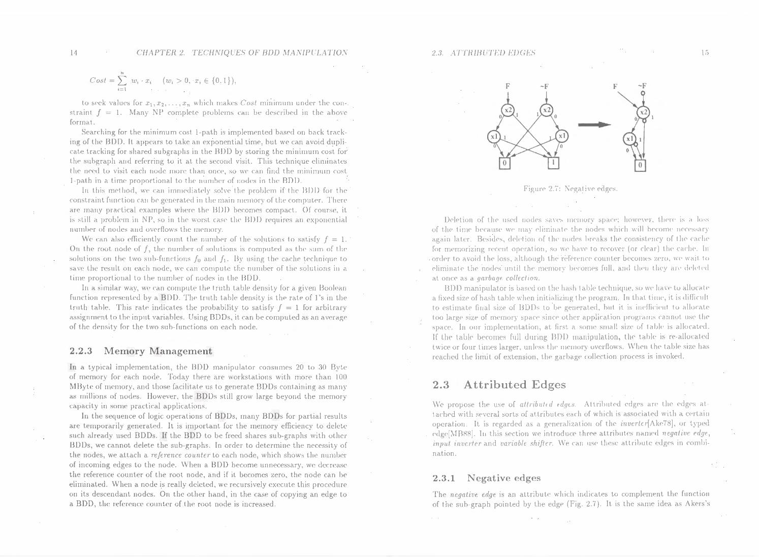
Figure· 2.7: f\'egati\e edges.

Oelf'tion of the used nodcs san·s nwmory span·; how<'\.<'r, t IH•re is a loss of the time bccausc we may eliminate the nodes which will become ncn·ss<uy again later. Besides, dclction of tlw nodes brcaks thc consistc·ncy of t lw cache for mc>morizing recent opc·ration, c;o we have to recover (or clear) the cache·. In order to avoid the loss, although the reference counter becomes zero, we• wait to eliminate the nodes until the memory lwcomc>s full, and tlwn th<"y an· d<·lct<-d

at once as a garbage collectwn. BDD manipulator is bas<'d on the hash table technique, soW<' h;n•<· to a! local<•

a fixed s1ze of hash table wben initializing the program. In that t.im<', it is difficult to estimate final size of BDDs to IH' genNated, but it is inc·fficic·nt to allocate too large s1ze of memory space since other application programs car1not use the

space. In our implementation, at first a some small size' of table is allocated.

If the table becomes full during BQJ) Jllanipu)ation, the ta\)Jp is IT-allocated twice or four times larger. unless thc m<>mory ovcrflows. \Vhcn thc table size has reached the limit of extension, the garbage collection process is invoked.

2.3 Attributed Edges

We propose the use of atlributrd ulgrs. Atlribulcd edge's are tlw <'dgcs at ­tached with several sorts of attributes each of which is associated with a c<•ttain operation. It is regarded as a gencrali7at ion of the invcrlc r[Akc78), or typed cdge[MB88]. Iu this section we introduce three attributcs narncd negalivr r>dgc, input inverter and variable sh1jlcr. We can use these attribute edgc·s in combi

nation.

2.3.1 Negative edges

The negative edge is an attribute which indicates to complement the function of the sub-graph pointed by the edge (Fig. 2.7). It is the same idea as Akers's

16 CHAPTER 2. TECHNIQUES OF BDD MANIPULATION

F G F G

Figure 2.8: Input inverters.

F F

•

Figure 2.9: An example where input inverters are effective.

inve7'le7·[Ake78) and Madre and Billon's typed edge[MB88]. The use of negative edges brings the outstanding merits as follows.

• We can reduce the size of BDDs to a half in the best case.

• Negation can be executed without traversing the g raph.

• Using the quick negation, we can accelerate logic operations with the ru les such as f · 7 = 0, f V 7 = 1, f Ef) 7 = 1, etc.

• Using the quick negation, we can transform the operations such as OR, NOR. NAND into AND by applying De Morgan's theorems, so that we can raise the hit rate of the cache to memorize recent operations.

2.3. ATTRIBUTED EDGES 17

F1 F2 Fl F2

•

Figure 2.10: Variable shifters.

Abuse of the negative edges breaks the important property that BDDs give canonical representation of Boolean functions. To keep this property, we place the following constraints on the location of the negative edges.

1. Do not use the 1-terminal node. Only use the 0-terminal node.

2. Do not use a negative edges on the l-edges .

These constraints are basically same as in Madre and Billon's work[MB88).

2 .3.2 Input Inverters

We propose another attribute indicating to exchange the 0- and l-edges at the next node (Fig. 2.8). It is regarded as complementing an input variable of the node, therefore we call it input inverter. Using input inverters, we can reduce the size of BDDs to a half in the best case. There are cases where the input inverters are very effective while the negative edges are not so effective (Fig. 2.9).

Since abuse of input inverters a lso break the property of giving a unique representation, we place a constraint as well as in using n<>galive <>dges. We use input inverters so that the two nodes fo and f 1 pointed by 0- and l-edges satisfy the constraints: (Jo < j 1 ), where '<' represents an arbitrary total ordNing of all the nodes. In our implementation, each edge id<>ntifi<>s the destination with the address of the node table, so we define the order as the value of th<> address. Under this constraint the uniqueness is maintained in a shared BDD.

2 .3.3 Variable Shifters

When there are the two subgraphs which are isomorphic except a diff<"'rence of their index numbers of input variables, we want to share them into one sub-graph by storing the difference of the indexes. To grant the request, we propos<"' variable

18 CHAPTER 2. 'I LC'/lz\JQ( ES OF BDD MANIJ>liLATIOS

shifter<;, which indicate to add a n111lliH'r to t.he indexes of its all descendant nodes. In this met hod, Wt' do not record an information oft he ind<•x on each nod<' because the' variable' shifter on each cdg<· ha\'<· a r<'lativc information bdween a pair of noclc·s. We plan• the following rul<·s to use variable shift<'rs.

On t.ll<' <•dg<' pointing a terminal nod<•. o not use a \'ariahl<• shift<>r

2. On t.hC' Nlg<! pointing the root nod<· of a BDD, the variabl<· shiftcr indicate's the ahsolut <' index number of the node.

3. Othcrwis<•, a variable shiftcr indicates the difference number of the index('s

bet w<'<'ll the start node and th<· cnd node of the edg<'.

For exarnpl<·, th<• graphs rC'presenting (.r1 V (x 2 • .r3)). (:r2 V (.r.3 · .r 1)) •... ,(l'k V

(.rk+l · .rk+·.d) <'<Ill he joined into tlw same graph as shown in Fig. 2.10. Using \'itriahl<• shifl<'rs. W<' can rC'clucc· tlw size of BDDs, <'.'q><'ciall) in the case

of manipulating a numher of regular functions, such as arithmetic sysiC'Jlls. The use of \'ariahl<· shift<•rs has anotlwr advantage that we can rais<> tlw hit rate of

the each<' of op<'l'at ions, hy applying the rule:

(f 0 9 h) {-==> {f(k) 0 g(k) = h(k) ),

where J(k) is a function whose ind<•:x<·s arc· shiftf'd by 1.· frotn .f. nnd o means a binary logic op<'rat ion such as 1 \/) OR, EXOU, etc.

2.3 .4 General Consideration

Here WC' !'how that, in general the' attrihut(•d <•dgt>s keep tlw prop<'rly of gi\'ing a

unique r<'J>n'scnt at ion of a Boolean function. The att rihut<•d <•dges can be dcvis<•d in the following manner. Let .':i be the

set of the Bool<'an functions of 11 inpuls.

1. Divide' s· into the two subset So and SI

2. Define a function :F: (S---+ S). such that for any f E 51 th<'ft' is a unique fo E .'·io to satisfy f = :F(fo ).

Namely, :F is tlw operation of the attributed edge, and the part it ion of S0 and S1 is related with the constraint on the location of thc attributed edges. \\'(' do not use attribut<'d edges pointing to a function in S0 . Using mathematical induction 011 th<· number of inputs 11, it is obvious that the attributed edge do not break the prop<•rty of uniqueness.

From the abo\'(' argument. we can <'xplain both of negative <'dgcs and input inverters. \lso variable shifters can b<.• <.•:xplaincd if we expand the argument as follows.

1. Partition S into a number of suhs<'ts S0 , 5 1 .... Sn.

2. For any k > I, Define a function :Fk: (S---+ S), such that for any f E Sk there is a unique foE So to sat isfy f :Fdfo).

2..1. l.\IPLE.\!ESTATIO\ \ND F\PERJ.\IE1\ rs HJ

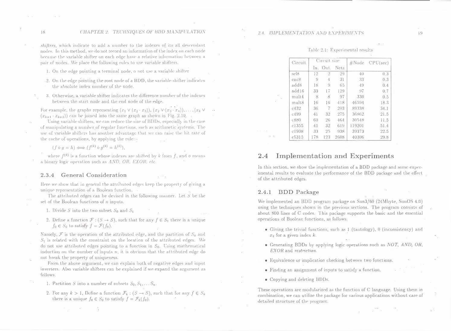
Tahk 2.1: Expcrimental n'sults

Circuit Circuit ~izc #':\ode C'PU(!-icc) In. Out. ~ets

sel8 12 2 29 40 0.3 enc8 9 -1 31 :33 0.3 add8 18 9 65 ·19 0.4 add16 :3:3 17 129 97 0.7 mult4 8 8 97 :l:W 0.5 mult8 16 16 418 46591 18.3 c432 36 7 203 89:338 :34.1 c499 41 :32 275 36862 21..5

c880 60 26 464 30518 11.5 c1355 41 32 619 119201 51.4 cl908 33 25 938 39373 22.5 c5315 178 12:3 2608 40306 29.8

2.4 Implementation and Experiments

In this section, we show the implementation of a BDD package and some cxpC'r­

imental results to evaluate the performance of the BDD package and tlH' cff<·<·t. of the attributed edges.

2.4.1 BDD Package

We irnplemented an BDD program package on Sun3/60 (24Mbyte, SunOS 4.0) using the techniques shown in the previous sections. T he program consists of about 800 lines of C codes. This package supports the basic and the csscnt led operations of Boolean functions. as follows.

• Giving the trivial functions, such as 1 (tautology), 0 (inconsistency) and

Xk for a given index k.

• Generating BOOs by applying logic operations such as NOT, AND, OH, EXOR and restriction.

• Equivalence or implication checking between two functions.

• Finding an assignment of inputs to satisfy a func:tion.

• Copying and deleting BODs.

These operations are modulariz<·d as the function of C' language. Using them in combination, we can utilize th<' packagf' for various applications without car(• of detailed structure of the program_

20 ('liAPTER 2. TEC/1 \'/Ql 'ES OF l3DD .\1. \.\'IPULATIOS

Table 2.2: F.ffc>ct of at tribut<'d edges

Circuit (A) (B) (G) (D) #Node CPU(scc #:\ode CPU #\ode CPt; #':\ode CPU

sel8 78 0.3 Sl o.:1 !)J 0.4 ·tO 0.3 c :nc~ 56 0.3 ·18 o.:l <18 0.3 33 0.3 acld8 119 0.4 81 0.4 81 0.4 49 0.4 aclciJ6 2:!9 0.7 161 0.6 I 6 l 0.7 97 0.6 mu I 1<1 524 0.5 <117 0 .. 5 400 0.4 330 0.5 rnult.8 66161 24.8 527.50 19.1 5050'1 19.8 46.594 18.3 cl! :12 l:lJ299 5.) .. 5 101066 36.S 1 o:J998 36.8 89338 34.1 <A !HJ ()9217 22.9 6.5671 2l.:l :wm~o 21.8 36862 21.5 <.;880 !)1019 17.5 31:378 10.8 :HHJ0:3 11.1 30.5'18 11.5 cl :1.55 212196 89.9 208:32·1 49.3 119·16.') 52.8 119201 .51.4 c I !)08 72537 :33.0 60850 21.6 :w:;:n 22.3 39373 ')') ~ --··) c!):JI!) 60316 31.3 483.53 29.2 ·11.') 12 28.6 10306 29.8

(r\)· Usmg noth1ng. ( B)· ( \)..L.. output ln\wters, (C): (B)+ input inverters. (D)· (C)+ variable shifters

In this package we implemented the attributed edges such as negative edges, input inverters and variable shifters. Thr storage requirement of this package is ahout 22 bytes a node. We can manage a maximum of about 700,000 nodes in our ma.rhinc.

2.4 .2 Experimental R esults

In ord<'r to cvaluat<' the efficiency of th<' program, we mad<' an experiment to g<'ll<'rate BDOs from combinational circuits. Notice that in this experiment the BDDs r<'prcs<'nt.s the set of the functions of not only primary outputs but all the internal nets. In order to count the numb<'t' of t IH• nod<'s f'xactly, we force to execute' garbage collection, which is unn<'ccssary in the practical use.

The• results arc shown in Table 2.1. The circuit .~c/8 is an 8-bit data sclecter. and t ne 8 is an 8-bit encoder. The circuits add'? and add 16 arc ~-bit and 16 bit add<'rs, and mult,f, mult8 are 1 bit and ~-bit multipliers. The rests are chosen from lwnchmark circuits in ISC AS '8.'>[BF85].

l'he sub column #Xodc shows th<' number of the nod<''i in the set of BDDs. Cf>l'(:;rc} shows t h<' total tinw of loading the circuit data, ord<'ring the input variables, and gc'n<'rating the BDDs.

The results show that we can quickly and compactly represent the functions of t ll<'s<' practical circuits. It took less than a minute to represent the circuits of dozcns of inputs and hundr<'ds of nets. \Vc can observe that the CPU time is almost proportional to thC' numbN of nodes. This manipulator is efficient enough wh<'n th<' size of f1DDs is feasible•.

2 .. 5. RE.\!ARI\5 ASD DJSCC<)S/0\S 21

In order to evaluate the effect of the at t rihut<•d <'dges. we made similar ex­periments by incrementally applying the l<'chniqucs. as shown in Table 2.2. The column (A) shows the results of the cxpcrinwnts using original BDDs without any attributed edges. The column (B) shows the results only us1ng negative edges. Comparing the results, we can oh::wrv<' that the m·gat ivc edges brings a maximum of about 40% reduction in tlw graph siz<' and outstanding spN•d up.

The column (C) shows the n·sults in add it ion to the input inverters to tlw (B). BDDs are reduced owing to the us<' of input inverters, and there arc no remarkable differences in CPU time. Espc•cially to th<' circuits c,f99, cl.'J.55 and cl 908, input inverters are effective and we can observe a maximum about 45% reductions of the graph size, although tlwy arc incffcctiv<' to some circuits.

The column (D) shows the rc•sults in adchtion to thC' variable shifters to the (C). BDDs are reduced still mor<' without n•markablc differC'nces of the C'J>lJ time. Variable shifterc; are effect i\'e' csp<'rlally to th<' circuit::. with the rc>gular structures, such as arithmetic logics \\'e• can also obsen·c· some degree of c•ffc>ds for other circuits.

The above results show that the• combination of the three attribut<'d cdgc•s arc much effective in many casc..o.;. though n<•it her of them is all-round <>ffc•ct ivc alone.

2 .5 Remarks and Discussions

In this chapter, we have shown the tcchniqucs of BDD manipulation. These t<'ch niqucs have been developed and improvc•d in .many la.boralori<'s in the world[Bry8(), MIY90, MB88, BRB90], and sonw program packagcs arc op<'IWd Lo public. Tlw techniques of the a.ttribut<'d edges havc lw<·n tried to improvC' the c·fficic·ncy of the programs. Especially, the nrgativc rdgc•s arc now commonly used bcrausr of their remarkable advantage. Using the BD)) packages, a numb<'r of works ar<' in progress on the VLSI CAD and ot hc>r various ar<'as in computer sciC'IICC'.

The novelty of BDD manipulation arc summarized as:

1. Extracting the redundancy which is containcd in the Boolean functions by using a fixed variable ord<'ring.

2. Completely removing the redundancy in tlw two rules: ''no duplicate nodes·' and ''no e•quivalcnt computation again''.

The algorithms of BOOs ar(' hasNI 011 I he• quick Sf'an h of the hash tahlc•s and the linked list data struct urc>. Both oft lw two te•dlfliques greatly bcnC'fit from the property of the random actf . .,.'i mar/mu modrl, such that any data on the· main memory can be accesscd in a ronst ant t inw. As most of computers ar<' d<'signcd in this model, we ran concludc· that th<' BD)) manipulation algorithms arc fairly sophisticated and adaptcd to I hC'! convc>ntional computer model.

22 CHAPTER 2. T£CllSIQl ES OF BDD .\1 \.\'IPUL.4.TJO.\'

Chapter 3

Variable Ordering for BDDs

3.1 Introduction

BOOs give canonical forms of Bool<'an functions provided that the order of in ­put variables is fixed. BDDs can hav<' many diffcr<'nt forms for a func-tion hy permuting the variables, and sometimes the siz<> of BOOs greatly varies with the order. The size of BOOs decid<'s not only memory requirement but also execution time for their manipulation. The variable ordering algorithm is one of the most important issues in the application of BOOs.

The effect of variable ordering depends on the kind of function to be handled. There are very sensitive examples that the B DO size vary extremely (exponen tially to the number of inputs) by only reversing the order. Such functions often appear in practical digital syst<'m d<'signs. On the other hand, there ar<' examples that the variable ordering is ineffective. For example, the symmetric functions obviously have the same form for any variable order. It is known that the function of multiplier[Bry91] cannot he represented by a polynomial-sized BDO in any order.

There are some works on the variabk ordc>ring. Concerning the method to find the exactly best order, Friedman et al. pr<'scnted an algorithm[F'S87] of O(n?3n) time based on the dynam1c programming, whc>re n is the number of inputs. It is still difficult to find the best order in a practical time for functions with many inputs, although this algorithm has been improved to the point where the best order can be found for some functions with 17 inputs(ISY91].

From the practical viewpoint, heuristic methods are intensively researched. ~1alik et al.[~1\VBSV88] and Fujita et ai.(FFK88] showed the heuristic methods based on the topological information of logic circuits. Butler et al. [BRKM91] uses testability measure for the heuristics, which r<'flC'ct not only topological but logical information of the circuit. These m<'thods arc to find a (may be) good order before generating BOOs. They arc applied to the practical benchmark circuits and compute a good ord<'r in many cases.

Fujita et al.[FMK91] showed another approach that improves the o rder for the given BOO by repeating the exchange of the variables. It can give further better

23

21J CllAP'J'EU .3. VARlt\f3DE ORDERING FOR BDDS

(a) Circuit. (b) In the- h<•st order. (c) In the worst. order.

Figure 3.1: BDDs for 2-level A:'-JD OR circuit.

r~:mlts than the initial BDDs, but som<'times it is trapped in local optimum. In this chaptN, we discuss the properties on th<' variable ordering for BDDs,

and show two heuristic methods of variable ordering which we have developed.

3.2 Properties on the Variable Ordering

Empirically, the following propNt ies arc observed on the variable ordering for BD Ds.

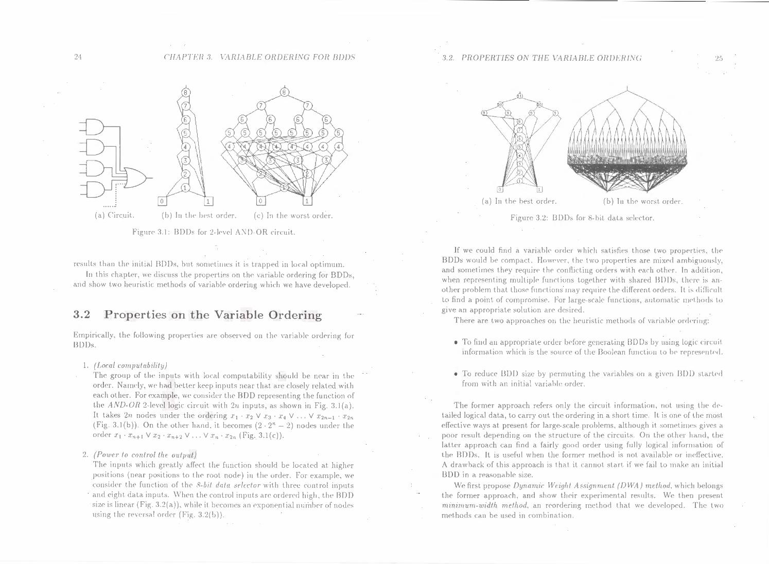
l. (Local compulablltty) The group of lh<' inputs with local computability should bc> near in the order. Nam<'ly, we had bcLt<'r keep inputs n<'ar that are closely related wit,h each other. l ~'or example, we consider the UDD representing the function of the AND-OR 2 level logic circuit with 2n inputs, as shown in Fig. 3.1(a). It takes 211 nodes under the ordering .r 1 • .r2 V .r3 • x 4 V ... V .r2n-J · .r2n

(Fig. 3.1 (b)). On the other hand. it becomes (2 · 2" - 2) nodes under the order .ft · .rn+l V :t·2 · .rn+2 V ... V :t"n · X2n (Fig. 3.l(c)).

2. (Powc1· to control the oulpul} The inputs which greatly aff<•ct the function should be located at higll<'r positions (rwar positions to th<' root node) in the order. For example. we consider th<' function of thC' 8-bit data ~rlrctor with three control inputs and eight data inputs. \\'h<'n the control inputs are ordered high, the BDD size is linear (Fig. 3.2(a)). while it becomes an <'Xponential number of nodes u:-~ing the rC'V<'rsal ord<'r (Fig. :l.2(b)).

3.2. PROPERTIES ON THE VARIABLE ORDERL'\G 25

(a) In the lwst ord~r. (b) In t lu• worst order.

Figure :3.2: ODDs for 8-h1l data s<'icctor.

If we could find a variable order which satisfies t hose• two propNtH•s, the BDDs would be compact. However, tlw two properties arc mixed ambiguously, and sorndimcs they require the conflicting orders with each other. Jn add it ion, when representing multiple> functions togcth<>r with sharc·d HODs, t lwre is an other problem that those' functions may r<'<ptire the different orders. It is clifTintlt to find a point of compromise. For large• scale functions, automatic nwt hods to give an appropriate solution are dcsirc•cJ.

There arc two approaches on the heuristic methods of variable orcl<•rillg:

• To find an appropriate order bcfore g<'ncraLing BDDs by using logic circuit information which is the source of th<· Boolean function to I><' n·prc·sc·nl<'d.

• To reduce BDD siz<' by permut.ing the· variables on a given BDD slartc>d from with an initial variable orcl<'r.

The former approach reft>rs only the circuit informal ion, not using t.he de­tailed logical data, to carry out the ordNing in a short tinw. It is on<' of the• most effective ways at presf'nt for large-scale problems. although it somf'tinws give's a poor result depending on the structure of the circuits. On the other hand, the latter approach can flnd a fairly good orde•r using fully logical information of the BDDs. It is us<>ful whC'n the forrne•r method is not available or inc•ffc•ctive. A drawback of this approach is that it cannot start if we• fail to mak<' an initial BDD in a reasonable si7.c.

We first propose Dynamic Weight Assignment (D WA) mdhod. which belongs the former approach, and show th<'ir <'Xpcrimental results. \Ve tiH•n present minimum-width method, an r<'ord<'ring method that we> dcvelop<'d. The two methods can be used in combination.

26 CJIAPTEH .1. VARIABLE ORDERING FOR BDDS

(a) First assignment.

... . (1) - ..... l. ................ J

(b) Second assignment.

Figure 3.3: Dynamic weight assignment method.

3.3 Dynamic Weight Assignment Method

When we utilize BDD techniques for digital system design, we first generate BDDs representing th<' functions for given the logic circuits. If tiH' size of the initial BDD is not fc•asible, we cannot p<'rform any O]H'ration of BDDs. Therefore, it is important for practical use to find a good order before gen<'rating BDDs.

Regarding the· properties on the \'ariable ordering of BDDs, we have dev<'l· opcd Dynamtc lVeighl Assignmfnl (DWA) method. In this method, the order is computed from the topological information of a given combinational circuit.

3.3.1 Algorithm

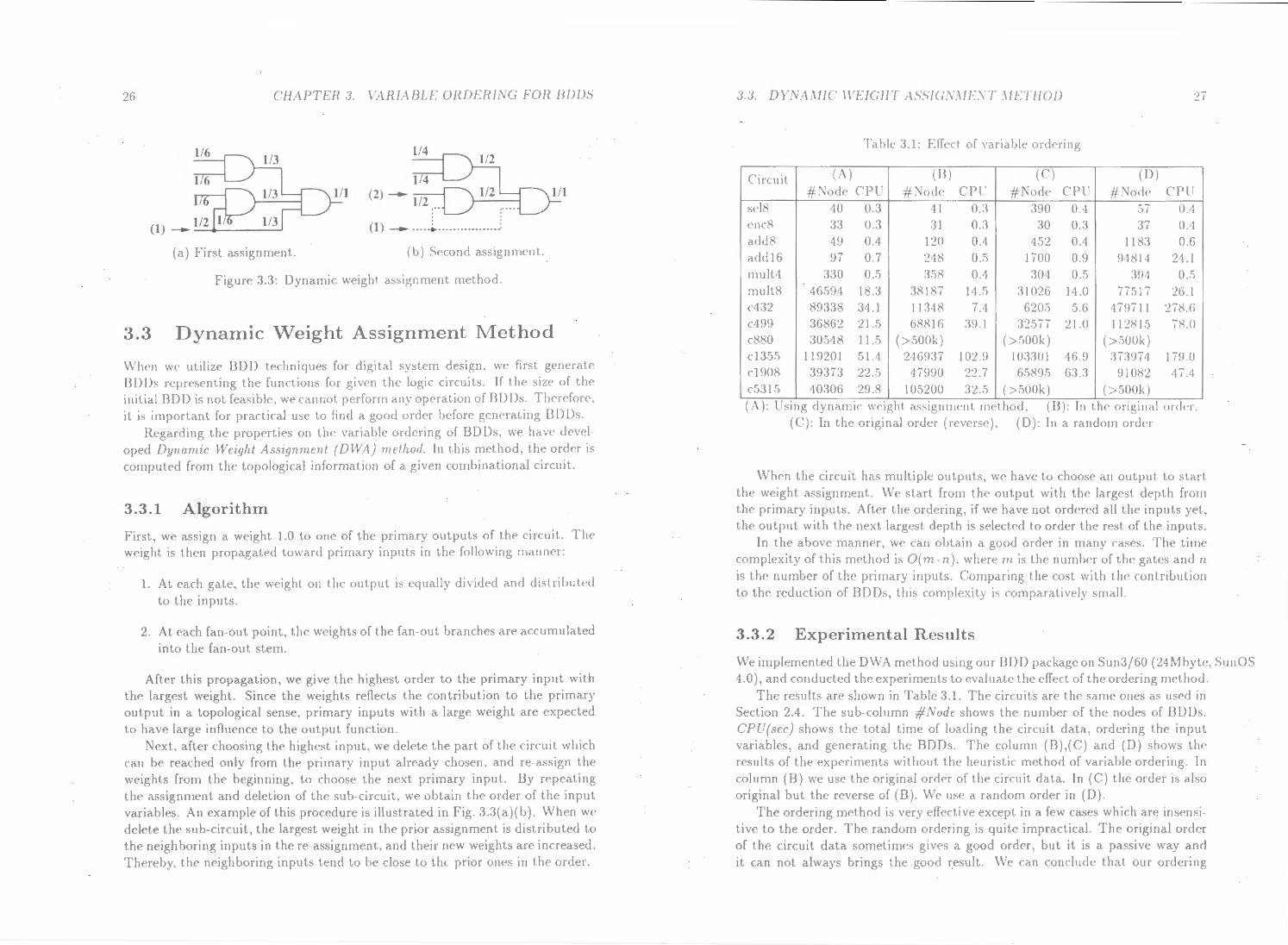
First, we assign a weight 1.0 to one of the primary outputs of th<> circuit. Th<' w<•ight is then propagated toward primary inputs in the following manner:

l. At each gate, the weight on the output is <'qually divided and distributed to the inputs.

2. At each fan-out point, the weights of the fan-out branches are accumulated into the fan-out stem.

After this propagation. we give the highest order to the primary input with thf' largest weight. Since the weights reflects the contribution to the primary out put in a topological sense, primary inputs \\.'ith a large weight are expected to have large inOucnce to the output function.

Next, after choosing the highest input, we delete the part of the circuit which can be reached only from the primary input already chosen, and re-assign the wc>ights from the bc>ginning. to choose the next primary input. By repeating the assignment and deletion of the sub-circuit, we obtain the order of the input variables. An example of this procedure is illustrated in Fig. 3.3(a)(b). When we dclct.e the sub-circuit, the largest weight in the prior assignment is distributed to the neighboring inputs in the re-assignment, and their new weights are increased. Thereby, the n<'ighboring inputs tend to be close to the prior ones in the order.

3.3. DYNAMTC H'EIG/lT ASSIGS.\11· .\'1 ,\IETIIOJJ

Table 3.1: Effect of variable ordering

Circuit (A) (B) (C) (])) #Node CPU #Node CPtJ #Node CPU #Node• CPU

sel8 40 0.3 41 o.:l 390 0. t 57 0.1 enc8 33 0.3 31 0.3 30 0.3 37 0..1 add8 49 0.4 120 0.·1 452 0..1 1183 0.6 add16 97 0.7 248 0.5 1700 0.9 9~811 21.1 mult1 330 0.5 358 OA 301 0.5 391 0.5 mult8 46594 18.:J 38187 11.5 31026 1" .0 77517 2G.I c432 89338 34.1 11348 7.4 6205 5.6 47~)711 278.6 c499 36862 21.5 68816 39.1 32577 21.0 112815 78.0 c880 30548 11 .. 5 ( >500k) {>500k) (>500k) cl355 119201 51.'1 246937 102 9 103301 16.9 :373971 17!).0 c1908 39373 22.5 47990 22.7 65895 63.:1 91082 17.1 c5315 40306 29.8 105200 32.5 (>500k) (>500k) .. (A): Csmg dynam1c wc1ght ass1gnnwnt method, (B)· In tlw ong111al orcl<•r,

(C): In the original order (revers<·). (D): In a random ordc•r

Wlwn the circuit has multiple outputs, W<' have to choose an output. to start the weight assignment. We start from thc> output with the largest dcpt h from the primary inputs. After the ordering, if we have not ordered all the inputs yet, the output with the next largest depth is selected to order the> rest of the inputs.

In the above manner, we can obtain a good order in many cases. The time complexity of this method is O(m · n), where m is the numh<'r of the gates and n is the number of the primary inputs. Comparing the cost with the contribution to the reduction of BDDs, this complexity is comparatively small.

3.3.2 Experimental Results

We implemented the DWA method using our BOO package on Sun3/60 {2~ M byt<', Sun OS 4.0), and conducted th<' experiments to evaluate the effect oft he ordering nwthod.

The results are shown in Table 3.1. The circuits are the same ones as used in Section 2.4. The sub-column #Node shows the number of the nodes of BDDs. CPU(sec) shows the total time of loading the circuit data, ordering the input variables, and generating the BDDs. The column (B),(C) and (D) shows tlw results of tlw experiments without the heuristic method of variable ord<'ring. In column (B) we use the original order of the circuit data. In (C) the order is also original but the reverse of (B). We usc a random order in ( D).

The ordering method is very effective except in a few ca<>es which ar<' in<><>nsi­tive to the order. The random ordering is quite impractical. The original order of the circuit data sometimes gives a good order, but it is a passive way and it can not always brings the good result. We can conclude that our ordering

28 CHAPTER 3. VARIABLE ORDERING FOR BDDS

Fl F2 F3

Figure 3.4: Width of BDDs.

method is useful and essential for many practical applications.

3.4 Minimum-Width Method

In this section, we describe another heuristic method of variable ordering based on the reordering after generating BDDs. In the following, n denotes the number of the input variables.

As a reordering method, Fujita et al.[FMK91] presented an incremental al­gorithm based on the exchange of a pair of variables (x;, x;+t)· lshiura et al [ISY91] also showed a simulated anealing method with the random exchange of two variables. These incremental search methods have a drawback that they greatly depend on the initial order. If the initial order is far from the best, many exchanges a re needed. This takes a long time, and there is the higher risk of being trapped in a bad local minimum solution.

We propose the method with another strategy. At first, we choose one vari­able based on a certain cost function, and fix it at the highest position (xn). Next, another variable is chosen from among the rest, and fixed at the second highest position (xn-d· In this manner, all the variables are chosen one by one, and they a rc fixed from the highest to the lowest. This algorithm has no back tracking. This method is robust to the variation of the initial order. In our method, we define the width of BDDs, as a cost function.

3.4.1 The Width of BDDs

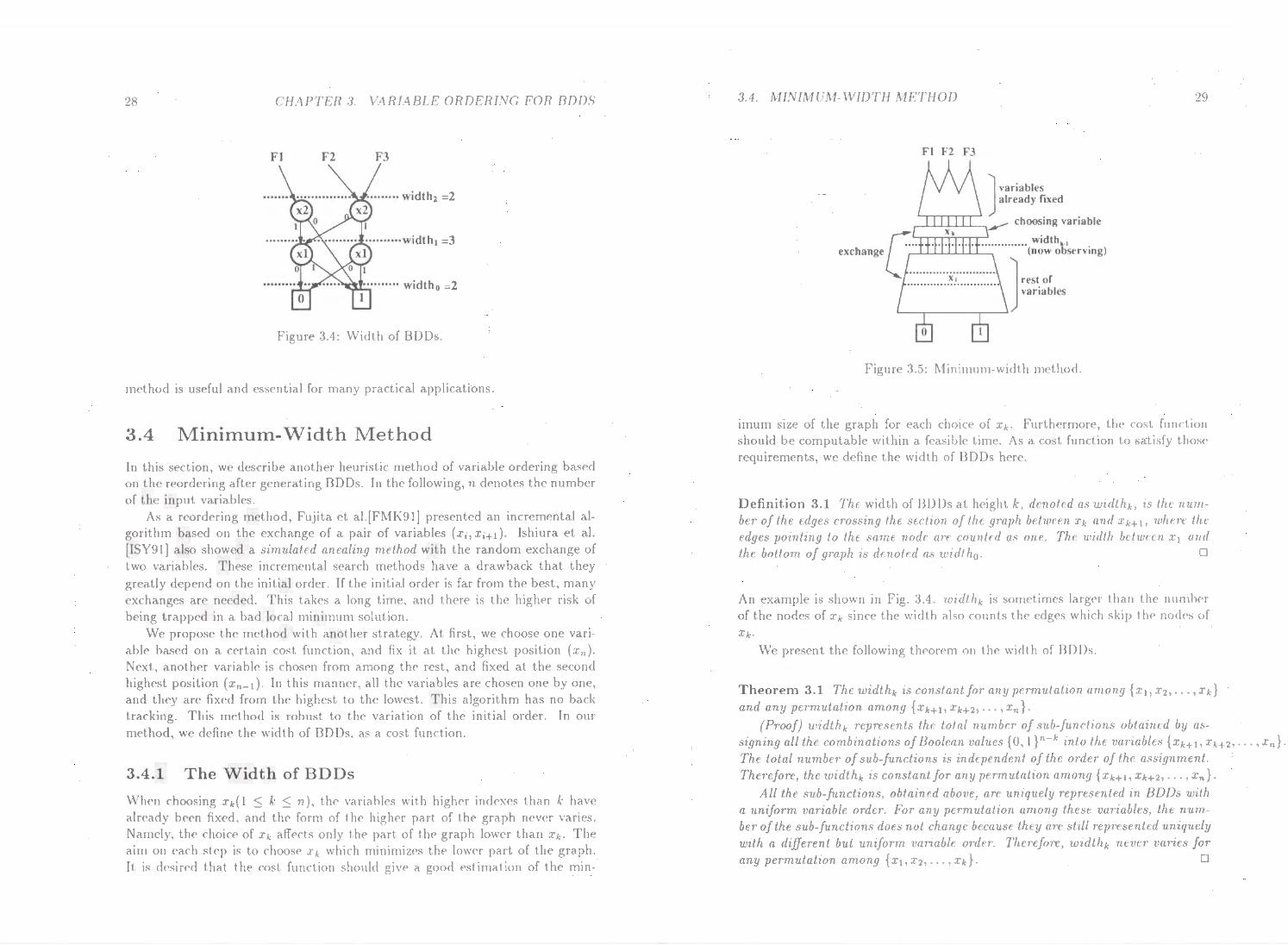
When choosing Xk(l ::; k ::; n ), the variables with higher indexes than k have already been fixed, and the form of the higher part of the gra.ph never varies. Namely, the choice of Xk affects only the part of the graph lower than Xk. The aim on each step is to choose J.'k which minimizes the lower part of the graph. It is desired that the cost function should give a good estimation of the min-

3.4. MINIMUM- ·wiDTH METHOD 29

Fl F2 F3

Figure 3.5: Minimum-width method.

imum size of the graph for each choice of Xk· Furthermore, th<' cost function should be computable within a feasible time. As a cost function to satisfy thos<' requirements, we define the width of BDDs here.

Definition 3.1 The width of BDDs at height k, denoted as widthk, is the num­ber of the edges c1·ossing the section of the graph between Xk and Xk+l, wher·e the edges pointing to the same node are counted as one. The width bclwcen x 1 and the bottom of graph is denoted as widt h0 . 0

An example is shown in Fig. 3.4. widthk is sometimes larger than the nurnbcr of the nodes of Xk since the width also counts the edges which skip the nodes of Xk·

We present the following theorem on the width of BDDs.

Theorem 3.1 The widthk is constant for any pe1mutation among { x 1, x2 , ... , xk}

and any permutation among { xk+ 1, xk+2• ... , Xn}.

(Proof) widthk represents the total number· of sub-functions obtained by as-signing all the combinations of Boo/em~ values {0, 1 }n-k into the variables {xk+ 1 , Xk+2, ... , l',J. The total number of sub-functions is independent of the order· of the assignment. Ther·efore, the widthk is constant for any permutation among { :z:k+l, Xk+2• ... , Xn}.

All the sub-functions, obtained above, are uniquely represented in BDDs with a uniform variable order. For any permutation among these var·iables, the num­ber of the sub-functions does not change because they are still rrp1·esentFd uniquely with a different but uniform variable order. Therefore, widthk never varies for any permutation among {x 1,x2 , ••• ,xk}. 0

30 CHAPTER .3. VAHIABLE OHDf;HJ.\'G FOR BDDS

3.4.2 Algorithm

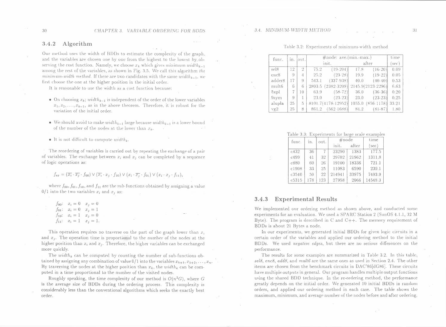
Our nwthod use~s the width of BODs to estimate the complexity of the graph, and tlw variables are chosen one by one from the highest to the lowest by ob­serving the cost function. I\amely, we choose Xi<- which gives minimum wzdihk_ 1

among the rest of the variables, as shown in Fig. :~.5. \\.'c> call this algorithm the 11WWTI!WI-wtdlh method. If there are two candidates with the same widthk-t, we first rhoos<' th<' one at the higher position in th<' initial order.

It is r<•asonable to use the width as a cost fun cl ion because:

• On choosing xk; widthk_ 1 is indcpcnd<'nt of the order of the lower variables .r 11 x2, ... ,xk-l, as in the above tlworem. Therefore, it is robust for the variation of the initial order.

• W<· should avoid to make widthk-l large because widlltk_1 is a lower bound of tlw number of the nodes at the lower than .r.k·

• It is not difficult to compute widlhk.

The reordering of variables is carried out by repeating the exchange of a pair of variabl<·s. 'fh<' <'Xrhange bet wecn l' 1 and x3 can be completed by a sequence of logic op<•rations as:

f~r = (Xi · X j · f oo) V ( x 1 • X j · !10) V ( l'j · X 3 · fo 1 ) V (X 1 • X J • !11),

wh<'r<' foo, fo1, !1o, and j,, are the sub-functions obtained by assigning a value 0/ I into th<' two variables x; and x 3 as:

foo: Xj = 0 XJ =0 fo1: Xi= 0 X 3 = 1 !JO: X;= 1 x3 = 0 fn: XI = 1 XJ = 1.

This operation requires no traverse on the> part of the graph lower than X 1

and xJ. The operation time is proportional to the number of the nodes at the higher position than .rl and xr Therefore. the higher variables can be exchanged rnor<' quickly.

Th<' 1c1dihk can be computed by counting the number of sub-functions ob­tained by assigning any combination of value 0/1 into the variables xk+1 , xk+2, ... , Xn.

By traversing the nodes at the higher position than xk, the widlhk can be com­puted in a time proportional to the number of the visited nodes.

Roughly speaking, the time complexity of our method is O(n2G), where G is th<' average size of BOOs during the ordering process. This complexity is considerably less than the conventional algorithms which seeks the exactly best order.

3A. MLVIMU.\1- \\'IDTH METJJOD 31

Table 3.2: Experiments of minimum-width method

fun c. m. out. #node: ave.(min.-max.) time in it. after (sec)

sel8 12 2 75.2 ( 19 201) 17.8 ( 16-20) 0.09 enc8 9 4 25.2 (2:l 28) 19.9 (19-22) 0.05 adderS 17 9 543.1 (337 938) 40.0 (40-40) 0.53 mult6 6 6 2803.5 (2382 3209) 2145.9(2123 2296) 6.63 5xpl 7 10 63.9 (58-72) 36.0 (36-36) 0.20 9sym 9 1 23.0 (23 23) 23.0 (23-23) 0.25 alupla 25 5 81 01 . 7 ( 4 1 7 8-1290 2) 1055.0 (856-1178) 33.21 vg2 25 8 861.2 (562-1688) 81.2 (81-87) 1.80

T bl 3 3 E t f a e JX penmen s or arg<' sea e examp es

func. m. out. #node time in it. after (sec)

c432 36 7 23290 1383 177.5 c499 41 32 29702 21962 1311 .8 c880 60 26 19100 18336 721.1 c1908 33 25 11083 6590 239.1 c3540 50 22 214941 33975 7493.9 c5315 178 123 27958 2066 14548.3

3.4.3 Experimental Results

We implemented our ordering method a.s shown above, and conducted s01m• experiments for an evaluation. W<' used a SPAHC Station 2 (SunOS 4.1.1, 32 M Byte). The program is described in C' and C++. The memory requirement of BOOs is about 21 Bytes a node.

In our experiments, we generated initial BOOs for given logic circuits in a certain order of the variables and applied our ordering method to the initial BOOs. We used negative edges, but th<'r<' are no serious differences on the performance.

The results for some examples are summarized in Table 3.2. In this table, se/8, enc8, add8, and mult6 are the same ones as used in Sc>ction 2.4. The other items are chosen from the benchmark circuits in DAC'86(dG8G]. These circuits have multiple outputs in general. Our program handles multiple output functions using the shared BOD technique. ln the r<' ordf'ring method, the performance greatly depends on the initial order. W<' generated 10 initial BOOs in random orders, and applied our ordering method in each case. The table shows the maximum, minimum, and average nurnb<'r of the nodes before and after ordering.

32 ClJ,\P'l /~H .1. VARIA EJI-E ORDERING FOR BDDS

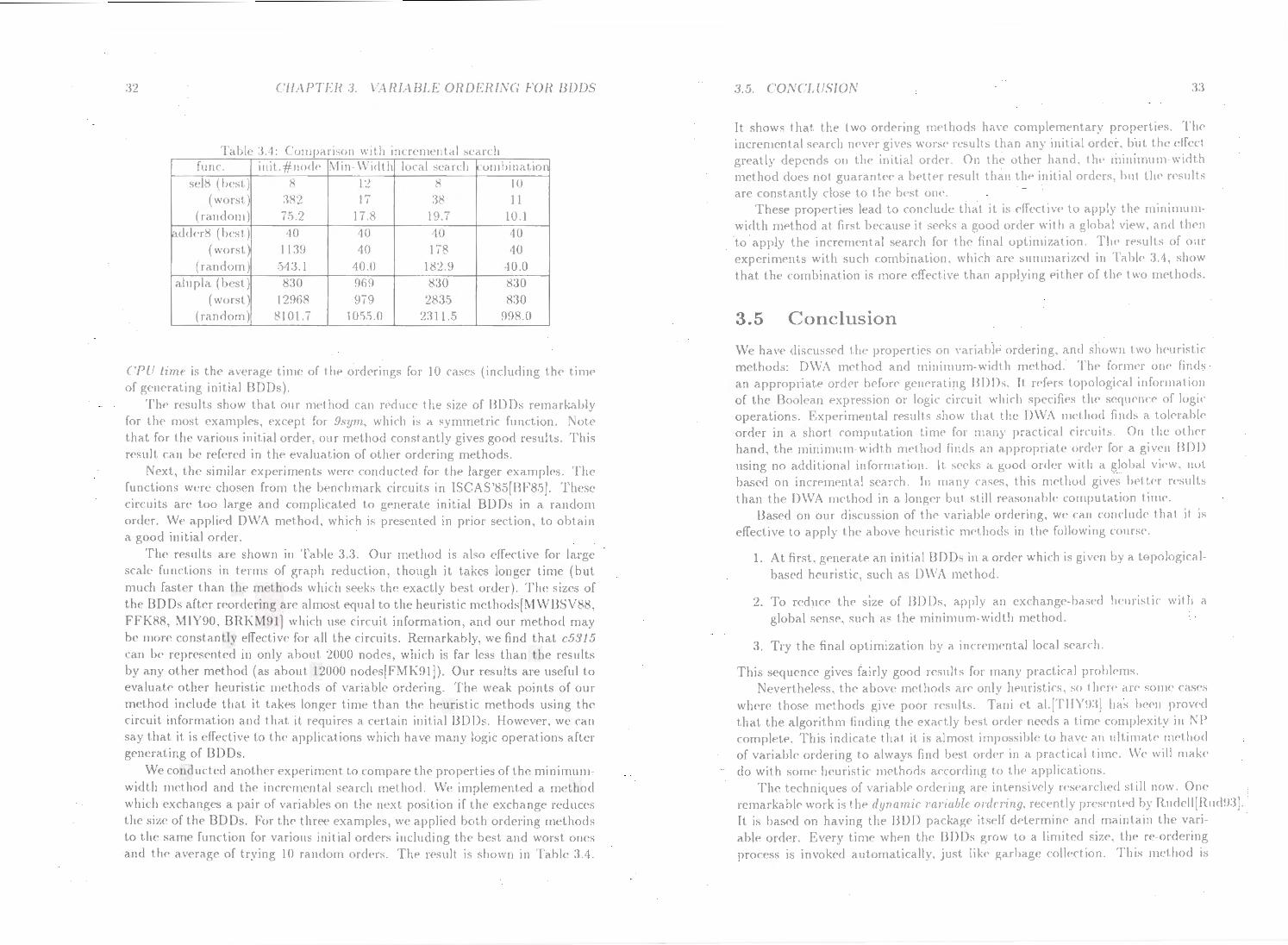
'I' ll 'l 1 c a J e , ·' : . h . Olllf>iHI:->011 Wit IIICfC'IIIC'Il t a searc 1

fun c. in it. #nod<• ~fin Width local search ·omhinatiot

sel8 ( he•st.) 8 12 8 10 (worst) 382 17 :38 11

{random) 75.2 17.8 I 9. 7 10.1

rtdd<'r8 {hest) 40 40 ·tO ·tO (worst~ 1139 40 178 ·10

(random) .)43.1 40.0 182.9 10.0 alupla (l><'st) 830 969 830 830

( \\'Orst 12968 979 2835 830 (random) 8101.7 1055.0 23 I 1.5 998.0

('/'(! hme is the av<'r'lge time of t.h<• orderings for 10 cases (inc:luding the time of g<'IICrating initial BDDs).

Tlw results show that our nwthod can rc>ducc the size of BDDs remarkably for t lw most f'XamplC's, except fo1 9~ym. which is a symmetric function. :\ote that for the various initial order, our method constantly gi,·es good results. 1 his result ran be ref<•rc•d in the evaluation of othN ord<•ring methods.

Next, the similar expcrim<'nts wNc conductNI for the larger examples. The fu11cl.ions were chosen from the benchmark circuits in ISCAS'85[BF8.1). These circuits are too large and complicated to gf'neratc: initial BOOs in a random ordc•r. We appli<'d OWA method. which is presented in prior s<'ctiou, to obtain a good initial order.

Th<' results are shown in Table 3.3. Our method is also eff<·ctivc for larg<' scale funct.ions in L<'rms of graph reduction, though it takes longer time (but mu rh faster than t h<• methods which seeks the exactly best order). The sizes of the B D Os after r<'orclcring arc almost equal to tlw heuristic methods[~l\VBSV88,

FFK88, MIY90, BIU~~191] which use circuit information, and our method may lw more constantly effective for all the circuits. Remarkably, we find that c5315 ran be represented in only about 2000 nodes, which is far less than the results by any other method (as about 12000 nodes[FM I\91]). Our results arc useful to evalua le other heuristic methods of variable ordNing. The weak points of our nwthod include that it takes longer time than the heuristic methods using the circuit informal ion and that it rcquir<'s a certain initial BDDs. However, we can ~ay that it is cff<'ctivc to the applications which have many logic operations after generating of BDDs.

WC' conducted a not her expe•rinwn I to compar<' I hC' properties of tlw mini mum­

width method and the incremental ~<'arch method. \\'e implemcntc>d a method whi<-h exchange~ a pair of variables on the next position if the exchange reduce's th<· s1ze of the> BDDs. For the tllr<"(' examples, we applied both ord<•ring methods to t.he same function for various initial orders including the best and worst ones and the average of trying 10 random ordC'r::;. The r<'sult is shown in Table :3. 1.

3.5. CONCLUSION 33

It sho"''S that the two ordering met hods ha \'C complenwnt ary properties. The incremental search nen'r gin•s worse rt'!..;ulb than any initial order, hut the c•ff<•ct greatly depends on the initial order. On l hC' other hand, t lw minimum-width method doe's not guarantt•ea bc>tter result than the initial orders, but tlw n•:-;ults are constantly close to the bc•st onf'.

These properties lead to conclude that it is dfectiV<' to apply the minin11tlll· width met hod at first bcraust' it seeks a good order with a global \'iew. and t hl'n to apply the incremental s<>arc:h for the final optimization. The results of our experinwnt s with such combination, \\ l11ch are summariz<·d in Tahl<' .l •I, show that th<' combination is more effect.tw than applying eit h~r of the two nwt hods.

3.5 Conclusion

\Ve have discussed t ht> pro pert ics on variabl<> ordering, ami shown two lwu rist ic methods: 0\VA method and minimum-width method. Tll(' form<'r <>IH' f111cls

an appropriate order bdorc gcnt"raling BDDs. It rcfC'rs topological informiiiJon of the Bool<•an expression or logic circuit which specifiC's t lH' seqll<'net• of logic operations. Experimental results show that the D\\'A nwthod finds a tolt·rahl<• order in a short computation time for 111any practical circuits. On the otht•r hand, the minimum-width m<'thod finds an appropriate ord<•r for a givc•n BDD

using no additional informal ion. it s<•cks a good order with a global vic·w, not based on incr<'mcntal s<'arch. In many cas<'s, this met hod giv<'s lwt tc•r rc·sldl.s

than the D\VA method in a longer but si ill reasonable colnputat ion I inw. Based on our discussion of the \·aria hi<' ordering, we• can conclude that it is

effective to apply the above heuristic nwt hods in the following course.

1. At. first, generate an init.ial BDDs in a order which is givc•n by a topologicfll·

basrd heuristic, such as D\VA method.

2. To reduce the size of BD Os. apply an exchangc-ba!:wd lwmist ic with a

global sense. such as the minimum·\\'idt h method.

3. 1 ry the final optimization by a inn<'nwnlallocal :-warclt.

This sequence gives fairly good results for many practical problems. NeV<•rthcless; the abO\<' methods arC' only hP-uristics, :-;o I lwrc arc• so11w cases

where those methods giv<· poor results. Tani et al.[ f'fiY!l:l) has l><·c·n pmwcl that the algorithm finding the c>xactly best. ordc>r needs a tinw compl<·xity in \'P complete. 'l his indicate that it is almost impossible to hew<· <lit ultimate nwtltod of variable ordering to always find best mcl<·r in a practical I inw. \VC' will make• do with some heuristic nwthods according to the applications.

The techniques of variable ordering arc· inl<'nsivcly rc•sc·arc:hc>cl si ill now. One remarkable work is the dyrwmir. 1·arwbh onlr ring. rc·cc·nt ly prc's<·ntC'd by H uciC'll[Ru(HJ:l]. It is based on having thf' BDO package• itsc•lf determin<• and maintain the• vari-able order. Every time> when the I3DDs grow to a lintitc·d siz<', UtP. re ordc•ring process is invoked automatically, just likc• garhagf' collN:t ion. This nwt hod is

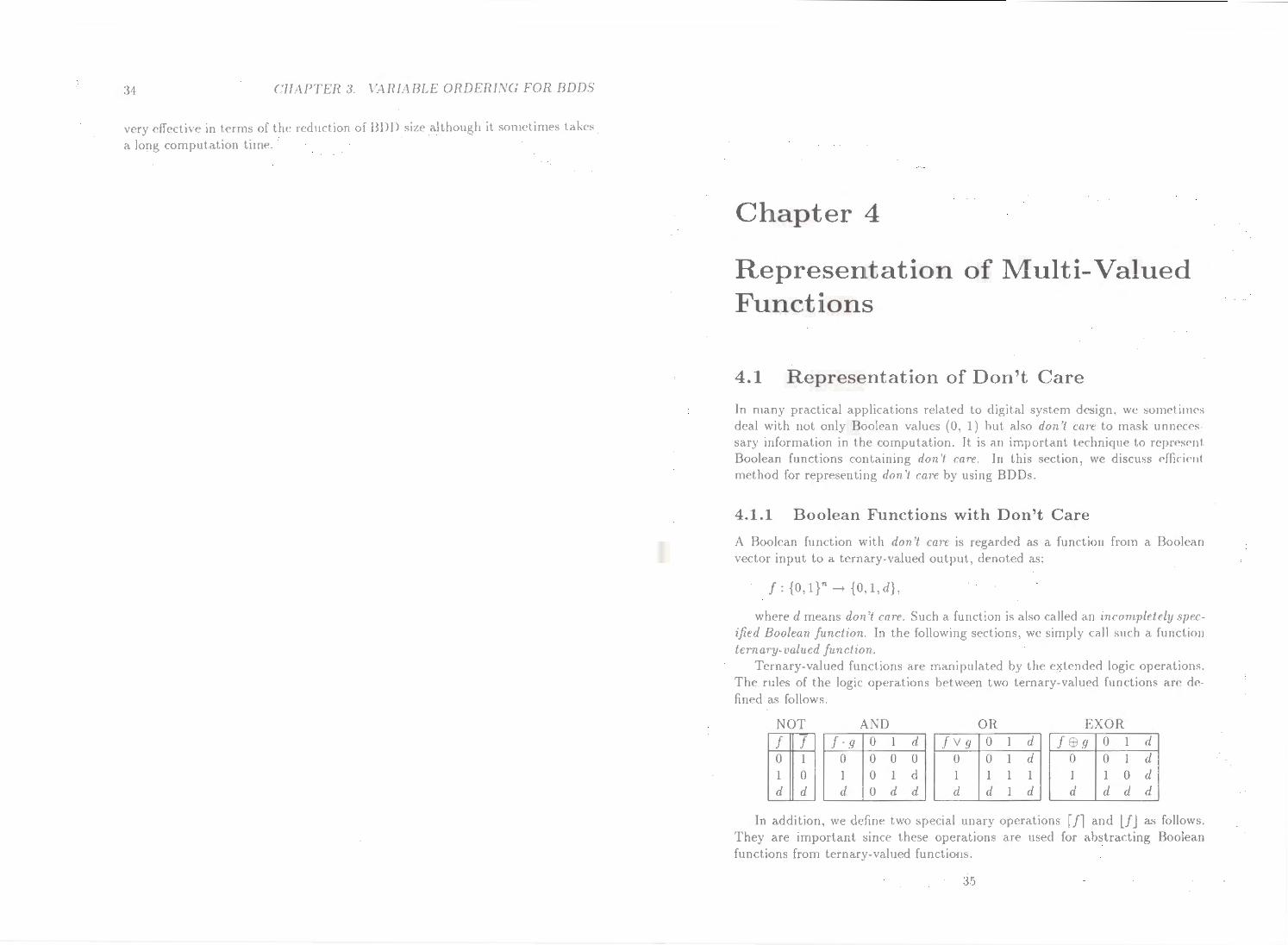
34 CHAPTER :J. \·:1\RIABLE ORDERI.\'G FOR BDDS

very effective in terms of the reduction of BDD size although it sometimes takes a long computation time.

Chapter 4

Representation of Multi-Valued Functions

4.1 R epresentation of Don't Care

In many practical applications related to digital system d<'sign, we sonwtinws deal with not only Boolean values (0, 1) but also don't ca1'e to mask UlliH'e<'s sary information in the computation. It is an important tcchnique to rcpr<'sent Boolean functions containing don 'I care. In this section, we discuss <'fficic•nt method for representing don 'I care by using BD Os.

4 .1.1 B o olean Functions with Don't Care

A Boolcan function with don't care is regarded as a function from a Boolean vector input to a ternary-valued output, denoted as:

f: {O,l}n--+ {0,1,d},

where d means don't care. Such a function is also call<'d an mcomplctcly .'>ptc­ificd Boolean function. In the following sections. we simply call such a function ternary-t•alued funclta1L

Ternary-valued functions arc manipulated by th<' <'Xt(•nded logic op<'ralions. The rules of the logic op<'rations between two ternary valu<'d functions arc d<' fined as follows.

AND OR EXOR f·g 0 1 d fVg 0 1 d jtf)g 0 1 d

0 0 0 0 0 0 1 d 0 0 1 d 1 0 1 d 1 1 1 1 1 1 0 d d 0 d d d d 1 d d d d d

In addition, we define two special unary operations ffl and l!J as follows. They arc important since these operations are used for abstracting Boolcan functions from ternary-valued functions.

35

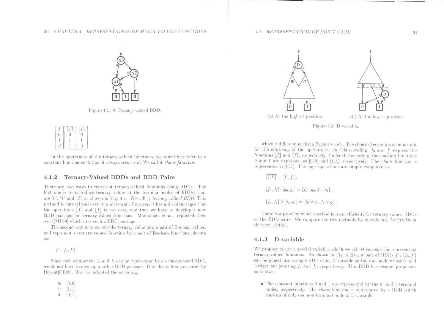
36 CHAPTER 1. HEPR1·5E.\ TAT/0,\ OF .\fULTI- VALUED FL".\'CT/0.\"S

Figure 4.1: A Ternary-valued BDD.

f Ul l!J 0 0 0 1 1 1 d 1 0

In the operations of the ternary-valued functions, we sometimes refer to a constant function such that it always returns d. We call it chaos function.

4.1.2 Ternary-Valued BDDs and BDD Pairs

There are two ways to represent ternary-valued functions using BDDs. The ftrst one is t.o introduce ternary values at the t<•rminal nodes of BOOs, that. are '0', '1' and 'd', as shown in Fig. 4.1. We call it ten1ary-vahud BDD. This method is natural and <'asy to understand. IIowcvN, it has a disadvantages that the operations r /l and l/J is not C'asy, and that we have to develop a new B DD package for ternary-valued functions. ~1atsunaga et al. reported their work[~1 F89] which uses such a BDD package.

The second way is t.o encodc the ternary-value into a pair of Boolean values, and represent a ternary-valuc•d function by a pair of Boolean functions, denote as:

f: [fo. /!].

Since f'ach component fo and f 1 can be rcpn•scntcd by an convf'nt ional BDD. we• do not have to d<'velop another BD J) package'. This idea is first prc>s<'ntcd by Bryant[C'B89]. liN<' we adopted the cnroding:

0: [0. 0] 1: [1.1] d: [0.1].

·1.1. REPRE8ESTA1 IOS OF DO\ ·y CARE :~;

f f

(a) At. the highc•st position. {h) At the low<'st pos1tion.

Figure 4.2: D-variablc•.

which is different one from Bryant 's code. The choice of <'ncoding is import ant for the efficiency of the• opcrat ions. In this encoding, fo and f 1 exprcss tlw functions l/J and r /l, respectivc·ly. Undc·r this <'ncoding, tlw constant functions 0 and 1 arc expressc•d as [0,0] and [1,1]. respectively. The· rhaos function is represented as (0.1]. 'I he logic opcrat ions are simpl) comput<·d as:

(Jo, fd · (go,gd = [fo · 9o, f, ·g.],

There is a problem which met hod is more efficient, the l<'mary valu<'d BDDs or the BDD pairs. We compare• the hvo methods by introducing D-l'ariablc in the next sect ion.

4.1.3 D-variable

Wf' proposC' to use a sp<'cial variable, which we call D-vanablc, for r<'(H'esf'nl ing ternary-vaht<'d functions. As shown in Fig. 4.2(a), a pair of BOOs f : [!0 , fd can be joined into a single BDD using 0 variable on the root node whos<' 0- and l -edges are pointing fo and f 1. resp<'cl tvc•lj. This BDD has c•legant propertic·s as follows.

• The constant functions 0 and 1 ar!' H'(>rCsc•rJt<'d by the• 0- and 1 terminal nodes, respectively. The• rhaos function is r<'(>resentc•d by a BDD which consists of only one non l<'rrninal nod<· of )) VMiable.

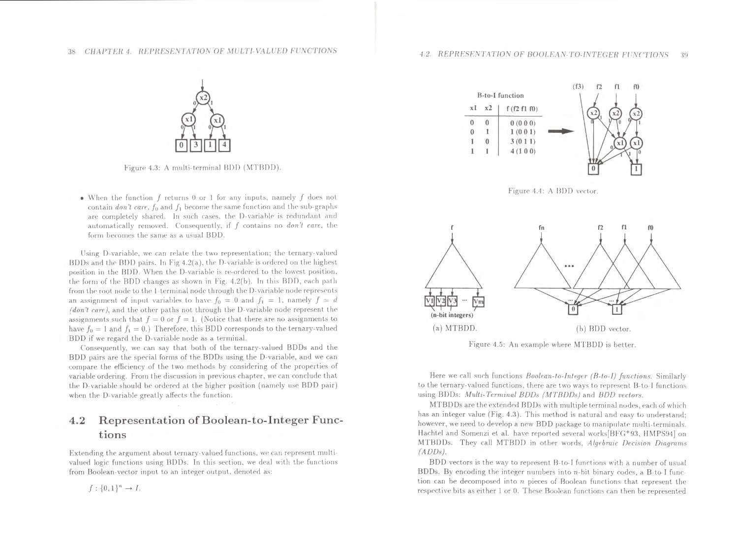
38 CIIAPTEH 4. REPRESESTATIOX Of \tULTI- VALUED FL'SCTIOJ\'S

Figure 4.3: A multi-t.crminal BD D (MTBDD).

• When the function f returns 0 or I for any inputs, namely f does not contain don 'l ca1·e, fo and f 1 become the same function and the sub-graphs arc completely shared. In -.uch cases, the D-\ariable is redundant and automatically removed. Con~equcntlv. if f contains no don 'I care, the form IJcromcs the same as a usual BDO.

Using D-variable, we can relate the two rcprcscntation; the ternary-valued BDDs and th<' BDD pairs. In Fig 4.2(a), the 0 -variablc is ordered on the highest position in the BDD. When the D-variable is re ordered to the lowest position, thc form oft he BOO changes as shown in Fig. 1.2(b ). In this BDD, each path from th<' root node to the !-terminal node through the D variable node represents an assignnwnt of input variables to ha\'c fo . 0 and j 1 = 1, namely f = d (don't ca1'c), and the other paths not through the D-variable node represent the assignnH·nts such that f = 0 or f = 1. (Notice that t here are no assignments to have fo 1 and f 1 = 0.) Therefore, this BDD corresponds to the ternary-valued BDD if W<' regard the D-variable node a..<; a tcrminal.

Consequently, we can say that both of the ternary-valued BDDs and the BD D pairs a re the special forms of the BODs using the D-variable, and we can compar<' the efficiency of the two methods by considering of the properties of variablc ordering. From the discussion in previous chapter, we can conclude that the D variabl<' should be ordered at the higher position (namely use BDD pair) when the D variable greatly affects the function.

4.2 Representation ofBoolean-to-Integer Func­tions

Extending the argument about ternary-valued functions, we can represent multi­valued logic functions using BDDs. In this section, we deal with the functions from Boolean-vector input to an integer output, denoted as:

J: {0, l}n-+ J.

·1.2. REPRESENTATIOS OF IJOOI E \S-TO ISTEGER F[ 'SCTI0.\'8 39

(f3) f2 n fO B-to-1 function

x1 x2 f (fl f1 fO)

0 0 0 (0 0 0) 0 1 1 (0 0 1) • 1 0 3 (0 11)

1 1 4 (1 0 0)

Figure 4.4: A BDD \'Cctor.

r fn f2 n ro

(n-bit integers)

(a) MT BDD. (b) BDD vector.

Figure 4.5: An example where MTB DD is better.

Here we call such functions Boolean-lo-Intcgcr (B-to-1) functions. Similarly to the ternary-valued functions, there arc two ways to represent B-to-1 functions using BDDs: Multi- Terminal BDDs (l1.fTBDDs) and BDD vrclors.

MTBDDs are the extended BDDs with multi plc t<'rrninal nodes, each of which has an integer value (Fig. 4.3). This method is natural and easy to understand; however, we need to develop a new BOO packag<' to manipu late multi-terminals. Ilachtel and Somenzi et al. haw• reportcd scv<'ral works{BFG+93, IIM P S94] on MTBD Ds. They call ~fTBDO in other words, Algebraic Decision Dwgrarns (ADDs),

BDD vectors is the way to represent B to I functions with a number of usual BDDs. By encoding the integer numbf'fs into n bit binary codes, a B-to-1 fu nc­tion can be decomposed into n pieces of Boolcan functions that represent t he respective bits as either 1 or 0. Thcs<' Boolean functions can then be represented

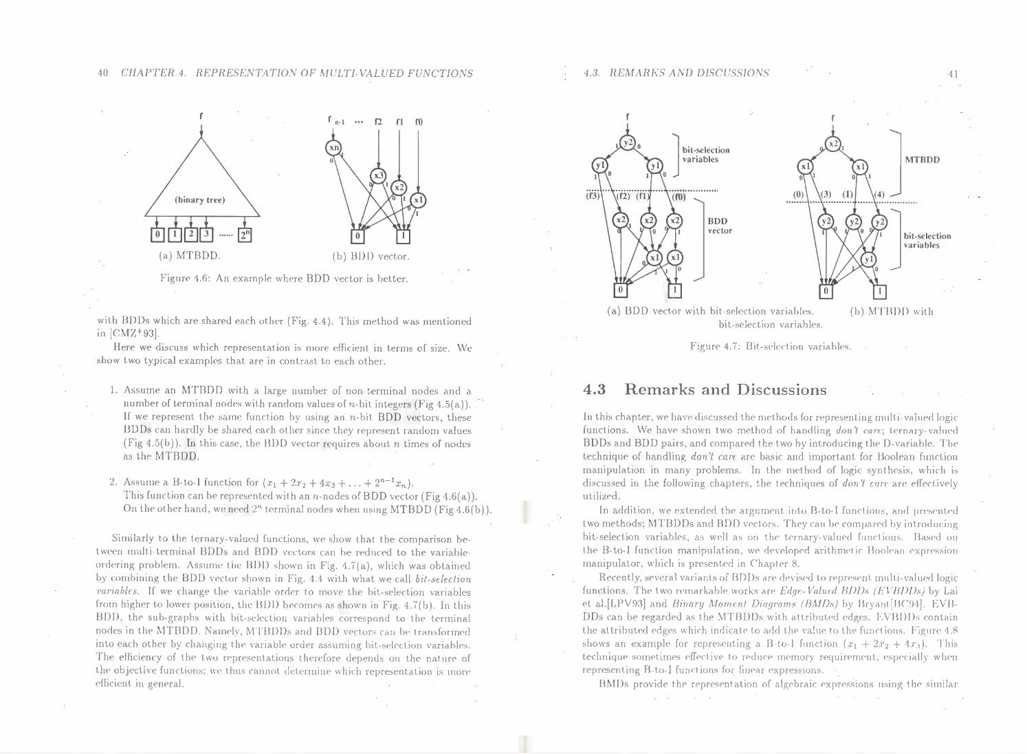
40 CHAPTER 4. REPRESENTATION OF MULTI-VALUED FUNCTIONS

r r n-1 f2 n ro

(a) MTBDD. (b) BDD vector.

Figure 4.6: An example where BDD vector is better.

with BDDs which arc shared each other (Fig. 4.4). This method was mentioned in [CMZ+93].

Here we discuss which representation is more efficient in terms of size. We show two typical examples that are in contrast to each other.

1. Assume an MTBDD with a large number of non-terminal nodes and a n umber of terminal nodes with random values of n-bit integers (Fig 4.5(a)). If we represent the same function by using an n-bit BDD vectors, these BDDs can hardly be shared each other since they represent random values (Fig 4.5(b )). In this case, the BDD vector requires about n times of nodes as the MTBDD.

2. Assume a B-to-1 function for (x1 + 2x2 + 4x3 + ... + 2n-lxn) · This function can be represented with ann-nodes of BDD vector (Fig 4.6(a)). On the ot.her hand, we need 2n terminal nodes when using MTBDD (Fig 4.6(b)).

Similarly to the ternary-valued functions, we show that the comparison be­tween multi-terminal BOOs and BDD vectors can be reduced to the variab le­ordering problem. Assume the BDD shown in Fig. 4.7(a), wh ich was obtained by combining the DDD vector shown in Fig. 4.4 with what we call bit-selection variables. If we change the variable order to move the bit-selection variables from higher to lower position, the BDD becomes as shown in Fig. 4.7(b). In this BDD, the sub-graphs with bit-selection variables correspond to the terminal nodes in the ~1TBDD. Namely, ~1TBDDs and DDD vectors can be transformed into each other by changing the variabl<' order assuming bit-selection variables. The efficiency of the two representations therefore depends on the nature of the objective functions; we thus cannot determine which representation is more efficient in general.

4.3. REMARKS AND DISCUSSIONS

r

J bit-selection variables

BDD vector

(a) BDD vector with bit-selection variables. bit-selection variables.

r

41

MTBDD

bit-selection variables

(b) MTBDD with

Figure 4.7: Bit-selection variables.

4.3 Remarks and Discussions

In this chapter, we have discussed the methods for representing multi-valued logic functions. We have shown two method of handling don't ca1·c; ternary-valued BDDs and BDD pairs, and compared the two by introducing the D-variable. The technique of handling don't care are basic and important for Boolean function manipulation in many, problems. In the method of logic synthesis, which is discussed in the following chapters, the techniques of don't care are effectively utilized.

In addition, we extended the argument into B-to-1 functions, and presented two methods; MTBDDs and BDD vectors. They can be compared by introducing bit-selection variables, as well as on the ternary-valued functions. Based on the B-to-1 function manipulation, we developed arithme1 ic 13ooiC'an C'xprC'ssion manipulator, which is presented in Chapter 8.

Recently, several variants of BDDs are devised to represent multi -valued logic functions. The two remarkable works are Edge- Valued JJDDs (EVBDDs) by Lai et al.[LPV93] and Binary Moment Diagrams (BMDs) by I3ryant[J3C94]. EVU­DDs can be regarded as the MTBDDs with attributed edges. EVBDDs contain the attributed edges which indicate to add the value to the functions. rigme 4.8 shows an example for representing a B-to-1 function (:r1 + 2:r2 + 4:r3 ). This technique sometimes effective to reduce memory requirement, especially when representing B-to-1 functions for linear expressions.

BMDs provide the representation of algebraic expressions using the similar

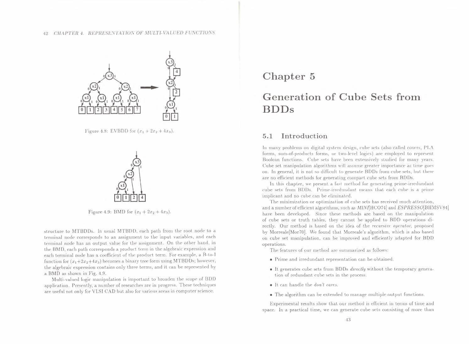
42 CHAPTER 4. REPRESENTATION OF MULTI- VALUED FUNCTIOSS

•

Figure 4.8: EVBDD for (x 1 + 2x2 + 4x3)·

Figure 4.9: BMD for (x1 + 2x2 + 4x3)·

structure to MTBDDs. In usual MTBDD, each path from the root node to a terminal node corresponds to an assignment to the input variables, and each terminal node has an output value for the assignment. On the other hand , in the BMD, each path corresponds a product term in the algebraic expression and each terminal node has a coefficient of the product term. For example, a B-to-I function for (x1 +2x2 +4x3 ) becomes a binary tree form using MTBDDs; however, the algebraic expression contains only three terms, and it can be represented by a BMD as shown in Fig. 4.9.

Multi-valued logic manipulation is important to broaden the scope of BDD application. Presently, a number of researches are in progress. These techniques arc useful not only for VLSI CAD but also for various areas in computer science.

Chapte r 5

Generation of Cube Sets from BDDs

5.1 Introduction

In many problems on digital system design, cube sets (also called covers, PLA forms, sum-of-products forms , or two-level logics) are employed to reprcs<'nt Boolean functions. Cube sets have be<'n extensively studied for many years. Cube set manipulation algorithms will assume greater importance as tim<> goes on. In general, it is not so difficult to generate BDDs from cube sets, but there are no efficient methods for generating compact cube sets from BD Ds.

In this chapter, we present a fast method for generating prime-irredundant cube sets from BDDs. Prime-irredundant means that each cube is a prime implicant and no cube can be eliminated.

The minimization or optimization of cube sets has received much attention, and a number of efficient algorithms, such a.s MINI{IIC074] and ESPRESSO(BIIMSV84] have been developed. Since these methods are based on the manipulation of cube sets or truth tables, they cannot be applied to BDD operations di-rectly. Our method is based on the idea of the recursive operator, proposed by Morreale[Mor70]. We found that Morreale's algorithm, which is also based on cube set manipulation, can be improved and efficiently adapted for BDD operations.

The features of our method are summarized as follows:

• Prime and irredundant representation can be obtained.

• It generates cube sets from BDDs directly without the temporary genera­tion of redundant cube sets in the process.

• It can handle the don't cares.

• The algorithm can be extended to manage multiple output functions.

Experimental results show that our method is efficient in terms of time and space. In a practical time, we can generate cube sets consisting of more than

43

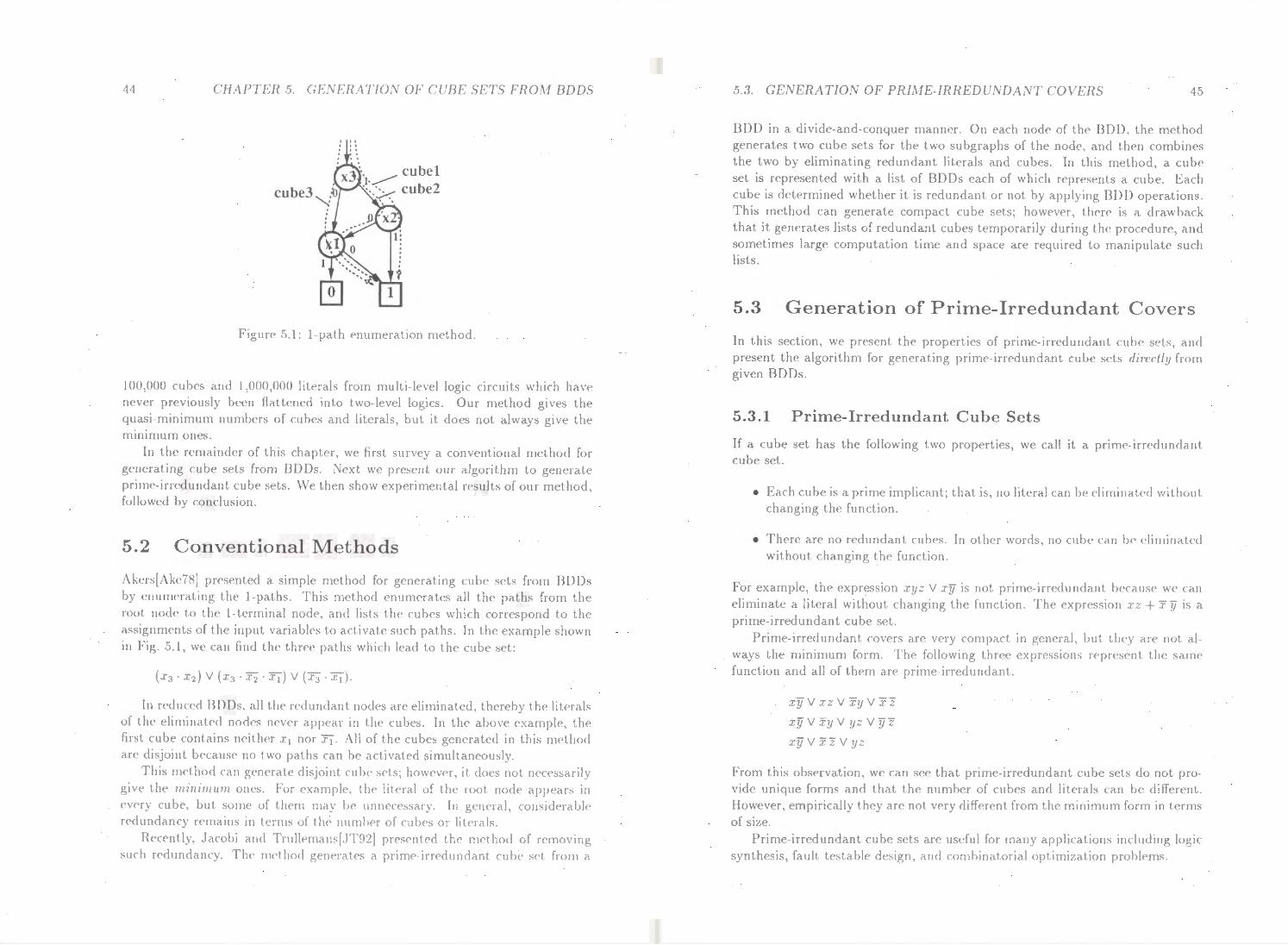
44 CHAPTER 5. GENERATION OF CUBE SETS FROM BDDS

Figure 5.1: 1-path enumeration method.

100,000 cubes and l ,000,000 literals from multi-level logic circuits which have never previously been flattened into two-level logics. Our method gives the quasi-minimum numbers of cubes and literals, but it does not always give the mmamum ones.

In the remainder of this chapter, we first survey a conventional method for generating cube sets from BOOs. Next we present our algorithm to generate prime-irredundant cube sets. We then show experimental results of our method, followed by conclusion.

5.2 Conventional Methods

Akers[Ake78] presented a simple method for generating cube sets from BDDs by enumerating the 1-paths. This method enumerates all the paths from the root node to the ! - terminal node, and lists the cubes which correspond to the assignments of the input variables to activate such paths. In the example shown in Fig. 5.1, we can find the three paths which lead to the cube set:

In reduced BDDs, all the redundant nodes are eliminated, thereby the literals of the eliminated nodes never appear in the cubes. In the above example, the first cube contains neither x 1 nor X!. All of the cubes generated in this method arc disjoint because no two paths can be activated simultaneously.

This method can generate disjoint cube sets; however, it does not necessarily give the minimum ones. For example, the literal of the root node appears in every cube, but some of them may be unnecessary. In general, considerable redundancy remains in terms of tlw numbf'r of cubes or literals.

Recently, Jacobi and Trullernans[JT92] presented the method of removing such redundancy. The met hod generates a prime-irredundant cube set from a

5.3. GENERATION OF PRIME-IRREDUNDANT COVERS 45

BDD in a divide-and-conquer manner. On each node of the BDD, the method generates two cube sets for the two subgraphs of the node, and then combines the two by eliminating redundant literals and cubes. In this method, a cube set is represented with a list of BDDs each of which represents a cube. Each cube is determined whether it is redundant or not by applying BDO operations. T his method can generate compact cube sets; however, there is a drawback that it generates lists of redundant cubes temporarily during the procedure, and sometimes large computation time and space are required to manipulate such lists.

5.3 Generation of Prime-lrredundant Covers

In this section, we present the properties of prime-irredundant cube sets, and present the algorithm for generating prime-irredundant cube sets di1·eclly from given BDDs.

5.3.1 Prime-Irredundant Cube Sets

If a cube set has the following two properties, we call it a prime-irrcdundant cube set.

• Each cube is a prime implicant; that is, no literal can be eliminated without changing the function.

• There are no redundant cubes. In other words, no cube can b<' eliminated without changing the function.

For example, the expr~ssion xyz V xy is not prime-irredundant because we> can eliminate a literal without changing the function. The expression xz + x y is a prime-irredundant cube set.

Prime-irredundant covers are very compact in general, but they an" not al­ways the minimum form. The following three expressions represent the same function and all of them are prime-irredundant.

xy V xz V xy V xz xy v xy v yz v yz xyv xzVyz

From this observation, we can see that prime-irredundant cube sets do not pro­vide unique forms and that the number of cubes and literals can be different. However, empirically they are not very different from the minimum form in terms of size.

Prime-irredundant cube sets are useful for many applications including logic synthesis, fault testable design, and combinatorial optimization problems.

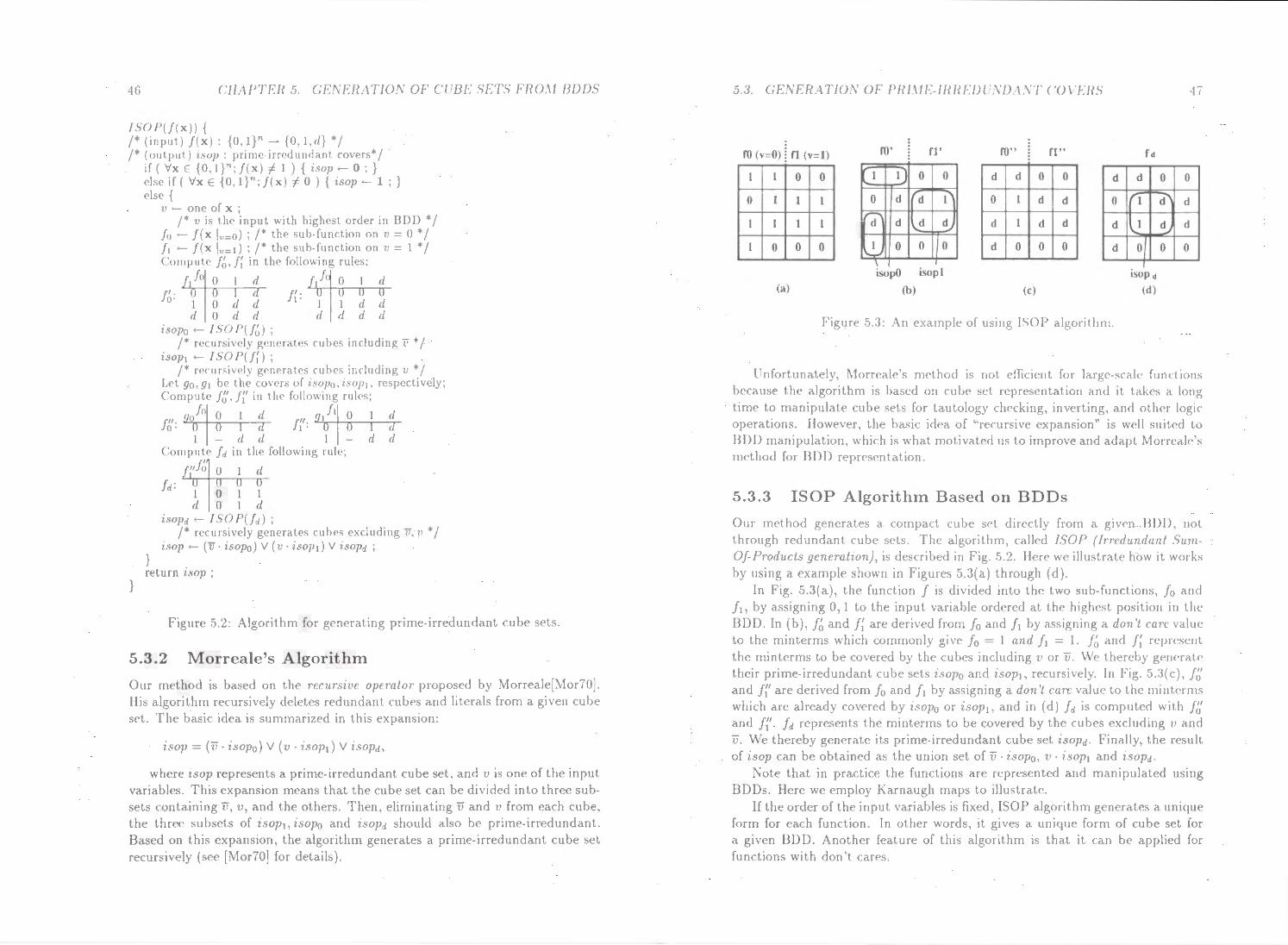
46 CHAPTER 5. GESEHAT/0.\' 01· Cl BE:. SET<> FR0,\1 BDDS

/SOP{f(x)) { /*(input) f(x): {0, l}n---.. {0, l,d} • / /*(output) u;op: primeirredundant covers*/

}

if { Vx E {o.l}n; f(x) f; 1 ) { iMp- 0 ; } <'lsc if ( Vx E {0, l}n; f(x) f; 0 } { isop- 1 ; } <'lse {

}

v - one of x ; /* vis the input with highest order in BDD • /

fo +- f(x lv=o) ; /* the sub-function on v 0 * / /1 +- f(x lv=I) ; /* the sub-function on v = 1 * / Corn put<' f~, J; in the following rules;

fo ~ .._]'n-hT---.T--n-

f~: I 0 d d d 0 d d

f '· t·

iMp0 • ISOP{f~);

1 d

1 d d d d d

/* rccursivcly generates cubes including F * / l80Pt - I SO P(f;) ;

/* recursively generates cubes including 1• • /

L~t g0 , g1 be the covers of isopo, isop1• respect h·cly; Cornput<' f(J, J:' in the following rules;

~ 0 h 0 (I/. ( !". .....,.,1 -+-rr----;,.-,-

JO • I·

l d 1 d Compute /d in the following rule;

/If~

fd: 1 0 1 1 d 0 l d

lSO]Jd +- ISOP(Jd) ; r rcc ll rsi vcly generates cubes excluding iJ, V *I l,'lop • (v · isop0) v ( v · isop1) v isopd ;

return i$Op ;

Figure 5.2: Algorithm for generating prime irredundant cube sets.

5.3.2 Morreale's Algorithm

Our method is based on the recurswc opera/01' proposed by Morreale(;\1or70]. Ilis algorithm recursively deletes redundant cub<'s and literals from a given cube set. The b·asic idea is summarized in this expansion:

1Mp = (v · isop0 ) V ( v · isopl) v isopd,

where t.c;op represents a prime-irredundant cube set, and vis one of the input variabl<.'s. This expansion means that the cube s<'t can be divided into three sub­sets ('Ontaining v, v, and the others. Then, eliminating v and v from each cube, the thr<'<' subsets of isop1, isop0 and isopd should also be prime-irredundant. Based on this expansion, the algorithm generates a prime-irredundant cube set r<'cursively (see [Mor70] for details).

.S.:J. GE.\'ERATIOS OF PRI.\IE-IRREDl \D \YI CO\'ERS

fO (v=O) l n (v=l) ro· fl' fO" 0" . 1 1 0 0 1 1) 0 0 d d 0 0 d

0 1 1 1 0 d d l 0 1 d d 0 ,.. 1 1 1 1 d d d d d 1 d d d

1 0 0 0 l 0 "-'

0 0 d 0 0 0 d \ isopO isopl

(a) (b) (c)

Figure 5.3: An example• of u::;ing !SOP algorithm.

d

1

1

0

isopd (d)

0 0

d d

d d

0 0

Vnfortunately, ~lorreale's met hod is not effici<•nt for large-scale functions because the algorithm is based on c:ubc s<•t r<•presentation and it tak<'s a long time to manipulate cube sets for tautology checking, inverting: and other logic operations. However, the basic idea of "recursive expansion" is well suit<'d to BOO manipulation, \'>'hich is what motivated us to improve and adapt Morreal~'s method for BDD representation.

5.3.3 ISOP Algorithm Based on BDDs

Our method generates a compact. cub<' s<'t directly from a given BOD, not through redundant cube sets. The algorithm, called /SOP (lrredundanl Sum­Of-Products generation), is dcscrib<'d in Fig. 5.2. Here we illustrate how it works by using a example shown in Figures 5.3(a) through (d).

In Fig. 5.3(a), the function f is divided into the two sub-functions, / 0 and / 1 , by assigning 0,1 to the input. variabl<' ordered at the highest position in the BUD. In (b), f~ and J; are derived from / 0 and / 1 by assigning a don 'I care value to the minterms which commonly g1vc fo =- I and / 1 = 1. f~ and J; represent the minterms to be covered by th<' cubes including v or v. We thereby g~n<•ral<' their prime-irredundant cube sets U>op0 and u.op1, recursivcly. In Fig. 5.3( c), Jg and J:' are derived from / 0 and / 1 by assigning a don't care value to the rnintcrms which are already covered by i.<;op0 or t.sop 1 , and in (d) fd is computed with/~' and f:'- /d represents the minterms to be covered by the cubes excluding v and v. We thereby generate its prime-irredundant cube set tSOPd· Finally, the result of zsop can be obtained as the union set of v · u;op0 , v · tsop1 and i.sopd.

Note that in practice the functions are represented and manipulated using BDDs. Here we employ I<arnaugh maps to illustrate.

If the order of the input variabl<'s is fixc·d, ISOP algorithm generates a unique form for each function. In other words, it gives a unique form of cube set for a given BDD. Another feature of this algorithm is that it can be applied for functions with don't cares.

·18 CHAPTER 5 GE:\'ERA110\ OF Cl BE SETS FR0.\1 BDDS

This algorithm is well suited for BD D op<•rat ions because:

• Tlw sub-functions fo and / 1 can be dcrivc•d from f in a constant time.

• Many redundant expansions can be avoided automatically because the re­dundant nodes are eliminated in rcduc<'d BDDs.

• BDDs cnables fast tautology ch<'cking, which is frequently performed m

the' procedure.

It is difficult to exactly evaluate the' time complexity of this algorithm. In our <'XJWrilllC'nts, as will be shown later, the' <'XCcution time was almost proportional to t.lw product of the initial BDD size and th<' final cube set size.

5 .3.4 Techniques for Imple mentation

In our algorithm, ternary-valued functions including the don't care value are ma­nipulated. As described in Chapter 'L 1. we r<'pre::;<•nt them with a pair of binary functions ( L!J' r Jl ). In this method, the tautology checking under a don'[ cart condition ran be written as rJl := l. The special operation for ternary-valued functions can be computed in the comhinat ion of ordinary logic operation for

lJJ and r Jl. For example, the ternary-valued operation:

! tj; 0 1 d

!~: 0 0 1 d 1 0 d d d 0 d d

can be written as:

( lf~J' r J~l) ~ ( lfoJ . r J,l, f!o 1) · W<• described earlier that isop is obtained as the union set of the three parts,

as shown in F ig. 5.2. In order to avoid cube set manipulation, we implemented tlu· method in such a way that the results of cubes arc directly dumped out to a fil<• On each r<'cursivc call, we push the procC'ssing literal to a stack, which we call a. rubf ~tar/.:. W hen a tautology function is detected. the current content of the r.ttbf· ~lad· is appended to the output file' as a cub<'. This approach is efficient because we can only manipulate BDDs. no matt<·r how large the result of the

c u hC' set bcconws. Our method can h<' cxtend<'d to manag<' multipl<' output functions. Sharing

tlw common nth<'::; among cltffcrcnt outputs. we obtain more compact represen­tation than if <'ach output WNC proc<'sscd sC'parat<>ly. ln om implementation, th<' cube sets of all the outputs arc g<'rH'ratNl concurrently; that is, in Fig. 5.2. W<' <'Xtcnd f to h<' an array of BDDs to repr<'!Wnt a multipl<' output function. lkp<'at.ing r<•cursiY<' calls in t h<' same manner a:; a single out put fund ion even­tuates in the detection of a multipk output constant which consists of O's and I 's. T he l's m<'an that corr<'sponding output fund ions include tlw cube which

is rum·ntlv k<'pl in th<' cube slack.

5.4. EXPERIMENTAL RESULTS 49

Table 5.1: Comparison with ESPRESSO

Name In. lOut. Our m<'thod ESPRESSO Cubes Literals fimc(s Cubes Lit. rrime(s

sel8 12 2 17 90 0.3 17 90 0.2 enc8 9 4 17 .56 0 •) .... 15 51 0.3 add4 9 5 135 819 0.7 135 819 1.9 add8 17 9 25 19 2-1211 13.3 2519 ~4211 443.1 mult4 8 8 145 945 1.4 130 874 5.0 mult6 12 12 2284 22274 26.7 1893 19340 1126.2 achil8f 24 1 8 32 0.2 8 32 2.0 achil8n 24 1 6561 59019 8.7 6561 59019 3512.7 5xpl 7 10 72 366 0.8 65 347 1.5 9sym 9 1 148 1036 0.9 87 60<) 10.7 alupla 25 5 2155 2Gn4 20.5 2144 ~6632 2.57.3 bw 5 28 68 :n.t 1.1 22 429 1.4 duke2 22 29 12G 12% :3.2 87 1036 28.8 rd53 5 3 35 192 o.:3 :31 175 0.5 rd73 7 3 14 7 1024 1.2 127 903 4.2 sao2 10 4 76 575 1.1 58 495 2.4 vg2 25 8 110 Hl ·1 1.9 110 914 42.8 c432 36 7 8423.5 969o:n 1714.8 X X >36k c880 60 26 114299 1986014 1096.6 X X >36k

5.4 Experimental Results

We implemented the method described in t h<· foregoing section, and conduct<'d some exper iments to evaluate its p<•rformanc<'. W<> us<'<l a SPA H.C Station 2 (Sun OS 4 .1.1. 32 M Byte). The program is writ tC'n in (' and C'++.

5.4.1 Comparison with ESPRESSO

First, we generated initial BDDs for t h~ out put func.tions of prac.t ical ccmthi­national circuits which may be multi-levt·l or lllldtipl<' output circuits. We· tiH•n generated prime-irredundant cube sc•ts from the BDDs and c.ountC'ci th<' numbc·rs of the cubes and literals. \\'e appli<'d t lw DWA ~1c·t hod. dt·snibC'd in St•ction :3.:3, to find the proper ord<'r of the input variahl<'s for tlu! initial BD D. ' I he com­putation time includes t.h<' time to clc•INmiru· otdc•ring, tlH' formatton of initial UDDs, and the time to generate prilll<:-irrc•clunclant cube sets.

\Ve compared our results with a conv<'nlional wbe-based mf'thod. We flat­t<'nC'd the given circuits into cube• s<'ls with the• syst<'m MIS- II [BSVW87], and then optimized the cube sets by J·,SP I Uo~SSO[B JJ MSV84}.

The results are shown in Table> !5.1. For circuits in this work wc appli<'d:

50 C'l/APTER 5. GENERAT/0.\ OF CTBE SETS FHOM BDDS

Table 5.2: Effect of variable ordering

~ame Heuristic order Random order

I#BDD Cubes Lit. ~imc(s) #BOO Cub<'.s Lit. l'i m<'( s)

sd8 16 17 90 0.3 41 17 90 0.3 cnc8 21 17 56 0.2 25 17 56 0.2 add8 41 2519 ~1211 13.:3 383 2319 24211 24.3 rnult6 1274 2284 ~2274 26.7 1897 2354 22963 30.2 achil8n 24 6561 '>9049 8.7 771 6561 59049 30.9 5xp1 4:3 72 :366 0.8 60 72 364 0.9 alupla 1376 215.5 ~6734 20.1 '1309 21.55 26730 43.1 lw.· 85 68 :n1 1.1 90 61 353 1.1 dukf'2 396 126 1296 3.2 609 125 1280 3.7 sao2 14:~ 76 57.5 l.1 133 76 571 1.0 vg2 108 110 914 1.9 1037 110 914 ') ... -·'

an 8-bit. data se]('(·tor (sel8), an 8-bit priority encoder (<'nc8), a 4+4 bit adder (add-1), an 8+8 bit adder (add8), a 2 x 2 bit multiplier {mult4), a 3 x 3 bit mu] tiplier (mult6), a 24 input Achilles· heel funclion(BH~1S\'84] (achil8p ). and its complement (achil8n). Other items were chosen from bf'nchmarks at MCr\C'90.

Th<' table shows that our method is much faster than ESPRESSO, with espc cially more than 10 times acceleration for the large scale circuits. The speed up was most impressive the c432 and c880, where we genf'ratf'd a prime-irredundant cube set consisting of more than 100,000 cubes and 1, 000,000 JitNals within a reasonable time. We could not apply ESPRESSO to th<'se circuits because we were unable to flatten them into cube sets even after ten hours. In another exam pie, ESPHESSO performed poorly for achil8n because the Achilles' heel funclwn requires a great many cubes when we invert it. Here, our method still puts in a good pNformance b<'cause thC' complementary function can be represented with the sam<· size BDD as the original one.

As far as the number of cubes and literals is concerned, our method in general may give somewhat. larger results than ESPH ESSO. In most cases, the differences range between 0% and 20%. In none of <'Xperiments, did we find an example giving more than two times the difference in terms of number of literals.

5.4.2 Effect of Variable Ordering

We conducted another experiment to evaluate the eff<'ct of variable ordering. In general, the size of llODs depends greatly on the order. \Ve generated prime­irredundant cube sets from th<' two BD Os of the same function but in a different order : one was in fai rly good order (obtained using the minimum-width method, shown in Section 3.4), and the other was in a random order.

5.4. EXPERL\1ES1 \ L RESt L 1 r; 51

Table 5.3: Result for variation of tlH' numb<•r of inputs ( 100 random function. single output

J

In. BDO size Cubes Lit<'rals Lit./ Cu he~ 1 0.58 0.77 1.:35 1.75 2 1.41 1.25 2.R1 ') •)-

___ , 3 3.22 2.30 7.17 :3.12 4 6.39 4.20 16.05 3.82 5 11.71 7.85 :36.39 4,64 6 20.51 14.88 82.18 5.52 7 36.24 27.09 172.06 6.35 8 64.59 r:•) ')"" ;) ___ / :377.41 -•)•} ,, __ 9 118.17 99.:31 808.09 8.14

10 210.12 192.26 17:18.89 ~).0 1 11 3().5.04 :370.90 :H)!J:3 .4 9 H.9G 12 633.97 722.11 7h65.91 10.89 13 1114.12 1106.31 166:35.79 11.83 14 2154.49 2752.53 351.54.84 12.77 15 4151.45 5:393.25 73980 .. 57 I :3.72

As shown in Table 5.2, the numbers of cubes and literals are almost the· sanw for both, while the size of BOOs varies greatly. The result demons! ral<•s that our method is robust for variation in order. Ilowever, vanable ordNing is still important because it affects the execution time and memory requirf'mc:nt.

5.4.3 Statistical Properties

Taking advantage of our method, W<' examined the statistical properties of prime irredundant cube sets. We applied our method to 100 pattc·rns of random func tions and took the average for the size of initial BOOs and generat<>d cube sets. The random functions were comput<•d using a standard C library.

Table 5.3 shows the property for variation 111 the number of inputs. Both DODs and cube sets grow exponc>ntially. It is known that the maximum BDD size is 0(2njn) (where n is the input number)[Ake78]. Our statistical <'Xperi­ment produced similar results. In t<•rms of number of cube<;, we obs<•rvc about 0(2n). The ratio of cubes to literals (the number of literals p<'r cub<>) is almost proportional to n.

Table 5.4 shows the property for variation in the numbcr of outputs whcn the numb<'r of inputs is fixed. Both BOOs and cube set-; grow a little less proportionally, appearing the effect of sharing their suhgraphs or cub<•s. \\'e expect suc.h data sharing is more effective in practical Circuits, since in many cases the output functions are relative each other, unlike random functions. The ratio of cubes to literals is almost constant, as the input number is fixed.

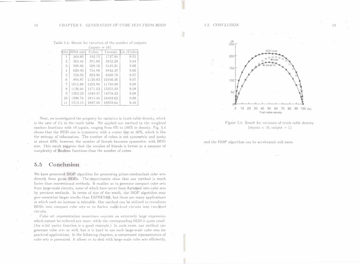
.)2 CHAPTER .5. GENER:\TIO.\ OF C'C.:BE SETS FR0.\1 BDDS

Table .'3.4: Result. for variation of the number of outputs (inputs = 10)

Out. BOD siz<' Cubes Literals .Lit./Cubes 1 209.80 192.13 1737.84 9.05 2 364.44 381.69 3452.20 9.04 3 500.86 568.10 5145.01 9.06 4 630.93 754.88 6842.25 9.06 5 758.33 933.86 8468.70 9.07 6 884.87 L 120.83 10166.36 9.07 7 1011.08 L 294.84 11750.90 9.08 8 1136.94 1171.63 13355.59 9.08 9 1262.29 1649.47 14978.33 9.08

10 1388.76 1815.44 16493.02 9.08 ll 1513.15 1987.56 18078.64 9.10

~<'xt. we investigatPd the property for variation in truth table density, whirh is the rat<' of 1 's in t h<' truth table. W<' applied our method to th<' weightc·d random functions with 10 inputs, ranging from 0% to 100% in density. Fig. 5.4 shows that t h<' BDD size is symmetric with a center line at 50%. which is like th<' entropy of information. 'I he number of cubes is not symmetric and peeks at. about 60%; how<>ver, the number of literals becomes symmetric with BDD s iz<'. This result suggests that the numb<'r of literals is better as a measure of complexity of Boo lean functions than the number of cubes.

5 .5 Conclus ion

WC' have prcs<'nted ISOP algorithm for generating prime-irrc>dundanl cube sets directly from given BOOs. Th<' expc>rimcnts show that our method is murh fastc>r than conventional methods. It enables us to generate compact cube sets from large-scale circuits, some of which have never been flattened into cube sets by previous methods. In terms of size of the result, the !SOP algorithm may gin• somewhat larg<'r results than ESPHESSO, but there are many applications in which such an increase is tolerable. Our method can be utilized to transform BDDs into compact cube s<'ls or to flatten mull i l<'vel rircuits into lwo-lcvc•l circuits.

Cube set rcpres<•ntat ion sonwtim<'~ r<•quires an extr<'m<'ly larg<' <'xpressJon which cannot be l'('(illn'd any more, while the corresponding BDD is q11ite small. (An n-bit parity function is a good example.) ln such cases. our method can g<'nerate cube sets as well, but it is hard to use such large-scale cub<' sets for practical applications. In the following chapters, a compress<'d representation of cube sets is pr<•sented. It allov-.·s us to deal with large-scale cube sets efficiently,

5.5. COXCLUSIOS

(I) 250

200

150

100

50

0 1 0 20 30 40 50 60 70 80 90 1 00 (%) Truth-table dens1ty

Figure 5.4: Result for variation of truth-table d<'nsity. (inputs = 10, output = 1)

and the ISOP algorithm can be accelerated still more.

53

54 CHAPTER 5. GESERATION OF CUBE SETS FROM BDDS

Chapte r 6

Zero-Suppressed BDDs

6.1 Introduction

Recently, BDDs have attracted much attention because they enable us t.o ma­nipulate Boolean functions efficiently in terms of time and space. There are many cases that the algorithm based on conventional data structures can be significantly improved by using BDDs[MF89, BCMD90).

As our understanding of BDDs has deepened, the range of applications has broadened. Besides Boolean functions, we are often faced with manipulating sets of combinations in VLSI CAD problems. By mapping a set of combinations into the Boolean space, they can be represented as a characteristic function using a BDD. This method enables us to implicitly manipulate a huge num­ber of combinations, which have never been practical before. Recently, new two-level logic minimization methods have been developed based on implicit set representation[CMF93). These techniques are also used to solve general cover­ing problems[LS90]. BDD-based set representation is more efficient than con­ventional methods. However , it can be inefficient at times because BDDs were originally designed to represent Boolean functions.

In this chapter, we propose a new type of BDD, which has been adapted for set representation[Min93b). This type of BDD , called a zero-suppressed BDD {0-sup-BDD), enables us to represent sets of combinations more efficiently than using conventional ones. We also discuss unate cube set algebra, which is con­venient to describe algorithms or procedures of 0-sup-BDDs. We developed effi­cient methods for computing unate cube set operations, and show some practical applications.

6.2 BDDs for Sets of Combinations

Here we examine the reduction rules of BDDs when applying them to represent sets of combinations. We then show a problem which motivates us to develop a new type of BD Ds.

55

56 C'll/\PTEH 6. ZEHO-Sl'PPHESSED BDDS

jump

(a) Node elimination. (b) Node sharing.

Figure 6.1: Reduction rules of conventional BODs .

... b f(a, b) = a b

··;··tHE f(a , b, c, d) = a b

1 0 1 01 11 10

00 0 0 0 0 b f(a, b, c) = a b •• c

01 0 0 0 0 a··... oo o1 11 10 o·m 11 0 0 1 1

1 0 0 1 1 10 0 0 1

Figure 6.2: Suppression of irrelevant variables in BO Ds.

6.2.1 R eduction Rules of BDDs

/\s mcnt ioned in Chapter 2, BOOs are basC'd on the following reduction rules.

l. Eliminate all the redundant nodcs whose two edges point to the same node. (Fig. 6.l(a))

2. Share all the equivalent sub-graphs. (Fig. 6.l(h))

BDDs give canonical forms for Bookan functions under a fixed variable or­ch•ring. ~lo!'lt oft he works on BODs are based on the• above reduction rules.

It is important how BDDs are shrunk by th<• r<•duction rules. One recent papt•r[LL92] shows that for general (or random) Book·an functions, node shar­ing makes a much more significant contribution to storage saving than node elimination. IIowcvcr, we consider that the node elimination is also important for practical functions. !:>or example, as in Fig. 6.2, llH' form of a BOO does not. dq><'nd on tllC' numb"'r of input variables as long as the expr<:>ssions of the

6.2. BDDS FOR SETS OF COMJJJNA'l'JO.\S

(abcd):{lOOO, 0100} (abc):{l OO, 010}

Figure 6.3: BDDs representing sets of combinations.

!)7

functions are the same. Using BOOs, the irrelevant variables are suppressed automatically and we do not have to consider them. This property is signifi­cant because sometimes we manipulate a function which depends on only a few variables among hundreds. This supprc•ssion comes from the node elimination of BDDs.

6 .2.2 Sets of Combinations

P resently, there have been many works on BDD applications, but some of them do not use BDDs to simply repr<'scnt Boolcan functions. wear<> oft<'n facc•d with manipulating sets of combinations. Sets of combinations arc used for describing solutions to combinatorial problems. We• ran solve combinatorial problems by manipulating sets of combinations. 'I he r<'J>r<'scntat ion and manipulation of sC'Is of combination are important techniques for many applications.

A combination among n items can !)(• rc•prc•scntcd by an n-bit binary VC'ctor , (.rn.rn-l ... x2 xt), where each bit, :rk E {l ,0}, c•xprcsses whether the correspond . ing item is included in the combination or not. A set of combinations can be represented by a set of then-bit binary \'eC"lors. Sets of combinations can be regarded as subsets of the power SC't on n itc·rns.

We can represent a set of combinations with a Boolc•an function by using n input variables for each bit of t.hc vc·ctor. Tlw output value of the function cxprC'sses whether each C"ombination spC'c.ifi(•d by thC' input variables arC' includC'd in the set or not. Such Boolcan fun et ions <HC' called rharactcrist1c function.<;. The operations of sets, such as union, intNscct ion and diffc•r<'ncc, can be execu ted by logic operations on charactNistic fund ions.

Using BO Os for characteristic functions, W<' can manipulate sets of combina­tion efficiently. In such BOOs, tlw paths from the· root node to the ]-terminal

58 CHAPTER 6. ZERO-SUPPRESSED BDDS

Jump

Figure 6.4: New reduction rule for 0-sup-BDDs.

node, which we call 1-palhs, represent possible combinations in the set. Because of the effect of node sharing, BDDs compactly represent sets of combinations with a huge number of elements. In many practical cases, the size of graphs becomes much less than the number of elements. BDDs can be generated and manipulated within a time that is almost proportional to the size of graphs, while previous set representations, such as arrays and sequential lists, require a time proportional to the number of elements.

Set manipulation using BDDs is very efficient, however, there is one incon­venience in that the form of BDDs depends on the number of input variables, as shown in Fig. 6.3. Therefore we have to fix the number of input variables before generating BDDs. This inconvenience comes from the difference in the model on default variables. In sets of combinations, irrelevant objects never appear in any combination, so default variables are regarded as zero when the characteristic function is true. Unfortunately, such variables can not be suppressed in the BDD representation. We have to generate many useless nodes for irrelevant variables when we manipulate very sparse combinations. Node elimination does not work well in reducing the graphs in such cases.

In the following section, we describe a method that solves the above problem by using BDDs based on new reduction rules.

6 .3 Zero-Suppressed BDDs

We propose the following reduction rules of BDDs to represent sets of combina­tions efficiently.

l. Eliminate all the nodes whose l-edge points to the 0-terminal node. Then connect the edge to the other subgraph directly, as shown in Fig. 6.4.

2. Share all equivalent sub-graphs the same as for original BDDs.

Notice that, contrary to the situation with original BDDs, we do not eliminate the nodes whose two edges point to the same node. This reduction rule is

6.3. ZERO-SUPPRESSED BDDS 59

(abcd):{lOOO, 0100} (abc):{lOO, 010}

Figure 6.5: 0-sup-BDDs representing sets of combinations.

asymmetric for the two edges, as we do not climina.te the nodes whose 0-edgc points to a terminal node.

We call BDDs based on the above rules Zero-Suppressed BDDs (O-s1tp-BDDs). If the number and the order of input variables are fixed, a 0-sup-BDD uniquC'Iy represents a Boolean function. This property is clear because a non-reduced binary tree can be reconstructed from a 0-sup-BDD by applying the reduction rule reversely.

Figure 6.5 shows 0-Sup-BDDs representing the combination sets which are the same ones shown in Fig. 6.3. A feature of 0-Sup-BDDs is that the form is independent of the number of inputs as long as the sets of combinations are the same. We do not have to fix the number of input variables before generating graphs. 0-sup-BDDs automatically suppress the variables which nevC'r appear in any combination. It is very efficient when we manipulate very sparse combinations.

For evaluating efficiency of 0-sup-BDDs, we conducted a statistical experi­ment. We generated a set of one hundred combinations each of which selects k out of 100 objects randomly. We then compared the size of both the 0-sup-BDDs and conventional BDDs representing these random combinations. The result for variation ink is shown in Fig. 6.6. This result shows that 0-sup-BDDs arc much more compact than conventional ones especially when k is small. Namely, 0-sup- BDDs are remarkably effective for representing sets of sparse combinations. The effect weakens for large k; however, we can use complement combinations to make k small. For example, the combination selecting 90 out of lOO objects is equivalent to selecting the remaining 10 out of 100.

Another advantage of 0-sup-BDDs is that the number of 1-paths in the graph is exactly equal to the number of combinations in the set. In conventional BDDs, the node elimination breaks this property. Therefore, we conclude that 0-sup­BDDs are more suitable than conventional ones to represent combination sets.

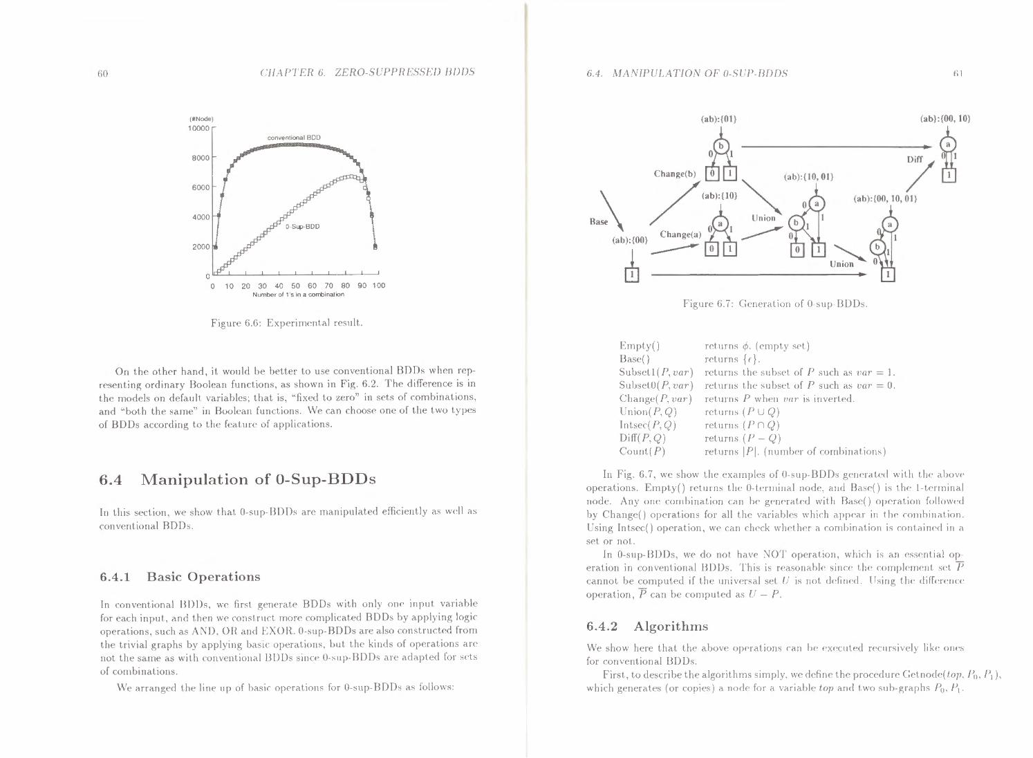
60

(MNode)

10000

CHAPTER 6. ZERO-SUPPRESSED BDDS

conventional BOO

0 1 0 20 30 40 50 60 70 80 90 1 00 Number of 1·s in a corrbination

Figure 6.6: Experimental result.

On the other hand, it would be better to use conventional BDDs when rep­resenting ordinary Boolean functions, as shown in Fig. 6.2. The difference is in the models on default variables; that is, "fixed to zero" in sets of combinations, and "both the same" in Boolean functions . We can choose one of the two types of BDDs according to the feature of applications.

6.4 Manipulation of 0-Sup-BDDs

In this section, we show that 0-sup-BDDs are manipulated efficiently as well as conventional BDDs.

6.4.1 B asic Operations

In conventional BDDs, we first generate BDDs with only one input variable for each input, and then we construct more complicated BD Os by applying logic operations, such as AND, OR and EXOR. 0-sup-BDDs are also constructed from the trivial graphs by applying basic operations, but the kinds of operations are not the same as with conventional BDDs since 0-sup-BDDs arc adapted for sets of combinations.

\Ve arranged the line up of basic operations for 0-sup-BDDs as follo.,vs:

6.4. MANIPULATION OF 0-SUP-BDDS f\1

(ab}: {00, 10}

/ (ab):{OO, 10, 01}

Figure 6.7: Generation of 0-sup-BDDs.

Empty() Base() Subsetl(P, var) SubsetO(P, var) Change( P, var) Union(?, Q) lntsec(P, Q) Diff(P, Q) Count(P)

returns </>. (empty set) returns { c}. returns the subset of P such as vm· = 1. returns the subset of P such as var = 0. returns P when var is inverted. returns (P U Q) returns (P n Q) returns (P- Q) returns IPI. (number of combinations)

In Fig. 6.7, we show the examples of 0-sup-BDDs genPrated with the abov<> operations. Empty() returns the 0-terminal node, and Base() is th<> 1-terrninal node. Any one combination can be generated with Base() operation followed by Change() operations for all the variables which appear in thP combination. Using Intsec() operation, we can check whether a combination is contained in a set or not.

In 0-sup-BDDs, we do not have NOT operation, which is an essential op­eration in conventional BDDs. This is reasonable since the compl<>ment set P cannot be computed if the universal set U is not defined. Using the diiTC'rcncc operation, P can be computed as U-P.

6.4 .2 Algorit hms

We show here that the above operations can be f'Xecuted recursively like ones for conventional BDDs.

First , to describe the algorithms simply, we define the procedure Getnode(top, P0 , P1 ),

which generates (or copies) a node for a variable top and two sub-graphs P0 , P1.

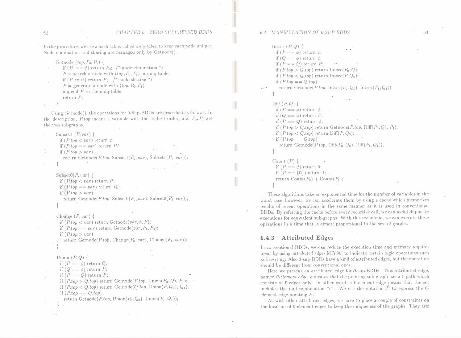
62 CHAPTEH 6 ZFHO Sl PPRESSED BDDS

In tiH' proo·durc. we use a hash table. called uniq-tablt. to k<'cp each node unique. \od<: elimination and sharing are managed only by Gct.node().

C:ct node (top, Po, P.) {

}

if (?1 ==</>)return P0 ; /*node elimination"'/ P = S('arch a node with (top, P0 , P1 ) in uniq-tablc; if (P exist) return P; /*node sharing*/ P- generate a node with (top, Po, PI); app(•nd P to the uniq-table; return P ;

Using G<'tnodc(), the operations for 0 Sup-BDDs arc described as follows. In the: d<'scription, P.top means a variable with the highest order, and Po. P1 are the two subgraphs.

Subset} (P,uar) {

}

if ( P.top < uar) return 6: if (P.Iop == var) return P1 ;

if ( P.top > var) return Get node( P.top, Subset l ( P0 • t·ar·). Suhsctl (Ph t•ar) );

Subsct.O(P,var) {

}

if (P.lop < var) return P; if (P.lop == var) return P0 ;

if ( P.top > var) return Getnode(P.top, SubsetO( Po, var), SubsetO( Pt, var) );

Change (P,var) {

}

if (P.top < var) return Getnode(um·,</>, P); if (P.lop == var) return Getnode(t•ar, P., Po); if ( P.top > vm·)

n•turn Getnode(P.top, Change(P0 , var), Change(?., var));

Union (P, Q) {

}

if (P == <P) return Q; if (Q == </>) return P; if ( P == Q) return P; if (P.top > Q.top) return Getnode(P.top, Union(P0 , Q), P1 ); if (P.top < Q.top) return Getnode(Q.top, Union(?, Qo), Qt); if (P.top == Q.top)

return Gctnode(P.top, Union(P0 , Q0 ), Union( PI, Ql ));

6.4. .\/ \SIPULATJOS OF 0-Sl J>-BDD.'-t

Intscc (P,Q) {

}

if (P == o) return 6: if (Q == <:>) return 9: if (P == Q) return P; if (P.top > Q.top) return lnts<'c(P0 , Q); if (P.top < Q.top) return Intsec(P,Qo); if (P.top == Q.top)

return Getnode( P.top, lntsec( P0 , Qo), lnts<'<·( P., Q. ));

Diff (P, Q) {

}

if (P ==</>)return </>;

if ( Q == </>) return P; if (P == Q) return </>;

if (P.top > Q.top) return Getnodc(P.lop, Diff(Po, Q), PJ); if (P.top < Q.top) return Diff(P. Qo}; if (P.top == Q.top)

return Getnode(P.iop. Diff(J>0 • Qo), Diff( P1, QJ) );

Count (P) { if ( P == 4>) return 0; if (P == {0}) return 1; return Count(P0 ) + Count(P1 );

}

These algorithms take an exponential time for the number of variables in the worst case; however, we can accelerate them by using a cache which memorizes results of recent operations in the same manner as it is used in conventional BDDs. By referring the cache before every recursive call, we can avoid duplicate executions for equivalent sub-graphs. With this technique, we can execute these operations in a time that is almost proportional to the size of graphs.

6.4.3 Attributed Edges

In conventional BDDs, we can reduce the execution time and memory require­ment by using attributed edges(~HY90J to indicate certain logic operations such as inverting. Also 0-sup-BDDs haw a kind of attributed edges, but the operation should be different from conventional oncs.

Here we present an attributed edg<' for 0 sup-BDDs. This attributed edge, named 0-clement edge, indicates that the polllting sub graph has a 1-path which consists of 0-edges only. In other wot d, a 0 element edge .means that the set includes the null-combination "c". We use the notation P to express the 0-element edge pointing P.

As with other attributed edges, we have to plac<> a couple of constraints on the location of 0-element edges to keep th<> uniqueness of the graphs. They are:

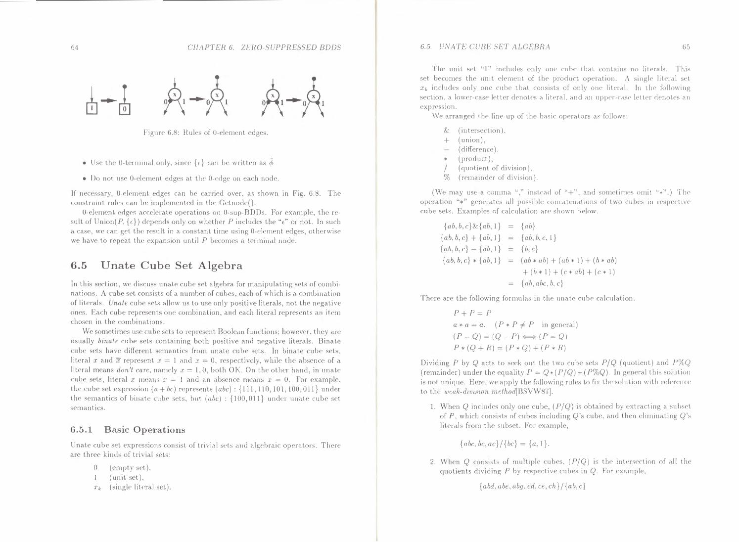
64 CJIAPTER 6. ZERO SL'PPRESSED BDDS

Figure 6.8: Rules of 0-element edges.

• Use th<• 0-tcrminal only, since { (} can be written as ~

• Do not use 0 clement edges at the 0-<'dge on each node.

If necessary, O·clcmcnt edges can be carried over, as shown in Fig. 6.8. The constraint rules can be implemented in the Getnode().

0-clcment cdgcs accelerate operations on 0-sup-BDDs. For example, the re­sult of Union(P, { c}) depends only on whC'ther P includes the "c" or not. In such a case, wc can get the result in a constant time using 0-element edges, otherwise we have to repeat the expansion until P becomes a terminal node.

6.5 Unate Cube Set Algebra

In this section, we discuss unate cube set algebra for manipulating sets of combi­nations. A cube set consists of a number of cubes, each of which is a combination of literals. lfnalc cube sets allow us to use only positive literals, not the negative ones. Each cube represents one combination, and each literal represents an item chosen in the combinations.

We sonwtinws use cube sets to represent Boolcan functions; however, they are usually bina/( cube scts containing both positive and negative literals. Binate cube sets have different semantics from unate cube sets. In binate cube sets, literal .r and 'I rcprescnt I = l and .r - 0, respectively, whil<' the absence of a literal means don 'I care, namely :r = 1, 0, both OK. On the other hand, in unate cube sets, literal .r means x = 1 and an absence means x = 0. For example, the cube set expression (a+ be) rcprc•sent s (a be) : { 111, 110, 101, l 00, 011} under the semantics of binate cube sets, but (abc): {100,011} undcr unate cube set semantics.

6.5.1 B asic Operations

U nate cuhc sd expressions cousist of trivial sets and algebraic operators. There arc three kinds of tnvial sets:

0 (empty set), 1 (unit set), l'k (single literal set).

6.5. UN:\TE CUBE SET ALGEHHA 65

The unit set ''1" includes only one cube that contains no literals. This set becomes the unit clement of the product op<•rat 1011. A single literal sd .r k i ncl udC's only one cube that consists of only on<' li tcr a I. In the following section. a lower-case letter dcnoks a literal. and an upper-case letter denotes an exprCSSIOn.

\\'c arranged the line-up of t h<' basic operators as follows:

& (intersection), + (union),

(cliff erence), * (product), I (quotient of division), % (remainder of division).

(\V<' may use a comma "," instead of "+". and sometimes omit "•" .) The operation "* '' generates all possible concatenalions of two cubes in resJWCt iv<· cube sets. Examples of calculation arc shown helow.

{ab,b,c}&{ab, 1} {ab, b, c} + {ab, 1} =

{ab, b, c} - {ab, 1} -

{ab, b, c} * {ab, 1}

{ab} {ab, b, c, I} { b, c}

(ab * ab) + (ab * I ) + ( b • ab)

+ ( b * 1) + ( c * ab) + ( c * 1) = {ab, a be, b, c}

There are the following formula~ in the unate cube' calculation.

P+P=P a*a=a, (P*P=fP ingcncral)

(P- Q) = (Q- P) <==> ( P = Q)

P * ( Q + R) = ( P * Q) + ( P * R)

Dividing P by Q acts to seC'k out the two cube sets PIQ {quotient) and /J(AQ (remainder) under the equality P- Q*(PIQ)+(PCXQ). In general thi~ ~olution is not unique. Here, we apply t lw following rules to fix the solution with rdcrcucc• to the weak-division mcihod[BSVW87).

l. WhC'n Q includes only OllC' cube, (PIQ) is obtain<'d by C'xtracling a suhs<'t of P, which consists of cubes including Q's cuiH', and then diminating Q's literals from the subset. For C'xample,

{a be, be. ac} I {be} = {a. 1}.

2. When Q consists of multiple' cubes, (PIQ) is tlw intc•rsection of all the· quotients dividing P by rC'spC'ctiv(> cubes in Q. For example,

{ abd, abe, abg, cd, cc, eh} I {ab, c}

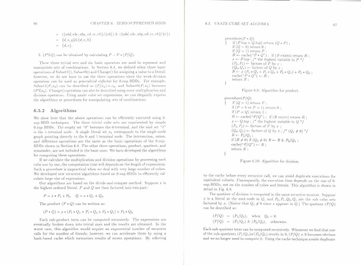
66 CHAPTER 6. ZERO-SL'PPRE88ED BDD8

= ( { abd. a be, abg. cd. cc . eh} I {a h}) & ( { abd. ab c. abg. cd. cc. eh} I { c})

- {d1 c,g}&{d,c.h}

- { d, ( }.

3. ( Po/r.Q) can b<' obtained by calculating P- P * (P /Q).

These three trivial sets and six basic operators are used to represent and manipulate sets of combinations. In Section 6.4. we defined other three basic op<'rations of Subset!(), SubsctO() and Change() for assigning a value to a literal; however, we do not have to use the three operations since the weak-division opcrat ion can be used as genc1·ahud cofactor for 0 sup-BOOs. For example, Subs<>tl(P,xk) can be described as (Pixk) * J'k. and SubsetO(JJ,.rk) becomes ( Po/t.rk). Change() op<'ration can also be described using some mull iplicat ion and di\·ision operators. Using unat<• cube set expressions. we can cl<'gantly express the algorithms or procedures for manipulating sets of combinations.

6.5 .2 Algorithms

We> show here that the above operations can be efficiently ex<'cutcd using 0-sup BDD techniqu<'S. The thre<' trivial cube sets are represent<'d by simple 0 sup BOOs. The empty set ''0" becomes the 0-terminal, and th<' unit set ''1" is th<' !-terminal node. A singl<' literal set Xk COJT<'Sponds to the single-node' graph pointing directly to the 0 and 1-terminal node. The intersection, union, and difference operations are the same as the basic operations of the 0-sup­BDDs shown in Section 6.4. The other three operations, product, quotient, and r<'mainder, are not included in the basic ones. We have developed the algorithms for computing these• operations.

If we calculate the multiplication and division operations by processing each cube one by one, the computation time will depends on the length of cxpressions. Such a procedure is impractical when we deal with very large number of cubes. We dcvdoped new n·cursive algorithms based on 0-sup-BDDs to efficiently cal­culate large size of cxpressions.

Our algorithms arc based on the divide-and conquer method. Suppose x is thc highest-ordered literal, P and Q are then factored into two-part:

P = x * P, + P0 , Q = x * Q. + Qo.

The product ( P * Q) can be written as:

(P * Q) = .r * (P. * Qt + P1 * Qo + Po * Q,) + Po * Qo.

Each sub-product term can be computed rccursively. The expressions are eventually broken down into trivial ones and the results are obtained. In the worst case, this algorithm would require an exponential number of recursive calls for the number of literals; however, we can accelerate them by using a hash-based cache which memorizes results of recent operations. By referring

6.5. UNATE Ct'BE SE1 ALGEBIL\

procedure(P,.. Q) { if (P.Iop < Q.top) rf'turn (Q * P) ;

if ( Q == 0) return 0 ;

}

if (Q = 1) return P; R f- each<>(" P * Q") ; if ( R exists) return R ; X f- P.top ; r the highcst variable in p *'I ( Po, P,) f- factors of P b\ .r ; (Qo,Qt) +- factors of Q 1;~ .r, R f- x ( P. * Q 1 + P1 * Q0 + P0 * Q.) + P0 * Q0 ;

cache('' P * Q'') f- R ; return R;

Figure 6.9: Algorithm for product.

procedure(PIQ) { if (Q =I) rc•turn P;

}

if ( P = 0 or P = 1) return 0 ; if (P = Q) return 1 ; R f- cachc("PIQ''); if(!? exists) return R; x f- Q.top ; /"' the higlwst variable in Q ·I ( Po, P.) f- factors of P by x ; (Qo,Qt) f- factors of Q by x; /* (Q 1 f. 0) *I R f- PtfQ1 ;

if (R =J 0) if (Q0 =J 0) R f- R & P0 IQ0 ;

cache(" PIQ") f- R ; return R;

Figure 6.10: Algorithm for division.

67

to the cache before every recursive call, we can avoid duplicate executions for equivalent subsets. Consequently, the ex<'cution time dcpC'nds on thc siz<· of 0-sup-BDDs, not on the number of cubes and literals. This algorithm is shown in detail in Fig. 6.9.

The quotient of division is computcd in the same recursive manner. Suppose x is a literal at the root-node in Q, and P0 , P 1, Q0 , Q 1 arc• the sub cui><' sets factored by .r. (Notice that Q 1 =J 0 since x appears in Q.) The quotient ( PIQ) can be described as:

(PIQ)

(PIQ) (Pt/Q. ), when Qo -= 0.

(P,IQJ) & (PoiQ0 ), otherwise.

Each sub-quotient term can be computed rccursively. Whenever we find that one of the sub-quotients (PtfQ.)or(P0 IQ0 ) results in 0, (PIQ) = 0 becomes obvious and we no longer need to compute it. Using the cache technique avoids duplicate

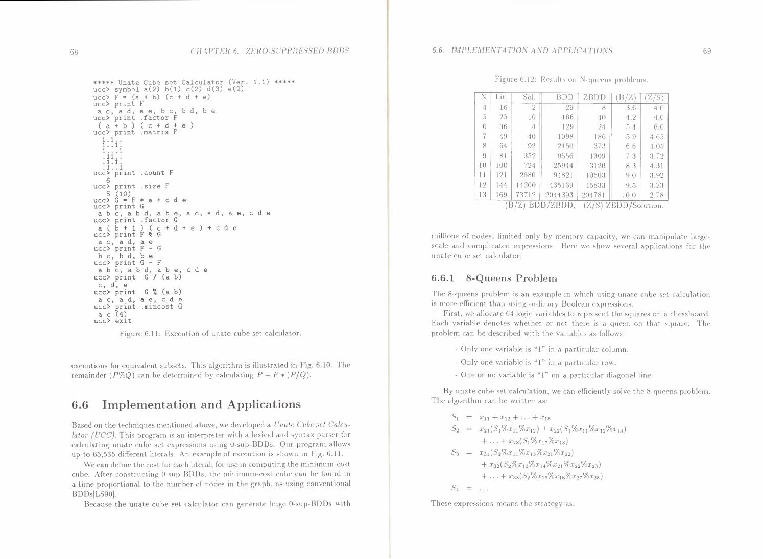
68 C//APTEH 6 lFHO Sl'PPRE'>8EO BOOS

***** Unate Cube set Calculator (Ver. 1.1) ***** ucc> symbol a(2) b(1) c(2) d(3) e(2) ucc> F = (a + b) (c + d + e) ucc> pr1nt F

a c , a d, a e, b c, b d, b e ucc> pr1nt .factor F

( a + b ) ( c + d + e ) ucc> print .matrix F

1.1.. 1..1. 1. .. 1 . 11 .. .1.1. . 1. .1.

ucc> pr1nt .count F 6

ucc> print .size F 5 (10)

ucc> G = F * a + c d e ucc> print G

a b c, a b d, a b e, a c, a d, a e, c d e ucc> print .factor G

a ( b + 1 ) ( c + d + e ) + c d e ucc> print F l G

a c, a d , a e ucc> pnnt F - G

b c , b d, b e ucc> print G - F

a b c, a b d, a b e, c d e ucc> print G I (a b) c, d, e

ucc> print G % (a b) a c, a d, a e, c d e

ucc> print .mincost G a c (4)

ucc> exit

Figure 6.11: Execution of unak cube set calculator.

cx<'cutions fo r equivalent subsets. This algorithm is illustrated in Fig. 6.10. The remainder (P%Q) can be determined by calculating P-P* (PJQ).

6.6 Implementation and Applications

Bascd on the techniques mentioned above, we dcvcloped a {'natc Cube set Calcu­lator (L'C'C). This program is an interpreter \Vith a lexical and syntax parser for calculating unate cube set expressions using 0-sup-BDDs. Our program allows up to 6.'>,5:35 different literals. An example of execution is shown in Fig. 6.11.

\\'e can dcfine the cost for each literal, for use in computing the minimum-cost cube. After constructing 0-sup-BDDs, thr minimum cost cube can be found in a time proportional to the number of nodes in the graph, as using conventional

BDDs(LS90]. Because the unate cube set calculator can general<' huge 0-sup-BDDs with

6.6. IMPLEME.YTATIOS ·\SO AJ>PLICA'J'/0\S 69

Figure 6.12: H<':,ltlts on \ qtH'<'lls probl<'ms.

X Lit. Sol. BDD ZBDD (B/Z) (Z/S) 4 16 2 29 ~ 3.6 4.0 5 25 10 166 40 4.2 4.0 6 36 4 129 2·1 5.4 6.0 7 49 40 1098 186 5.9 4.65 8 64 92 21.10 :n3 6.6 4.05 9 81 352 9556 1:!09 7.3 3.72

10 100 724 25914 :3120 8.:3 4.31 11 121 2680 94821 10.103 9.0 3.92 12 144 14200 4:35169 158:3:3 9.5 3.23 13 169 73712 2041:39:3 201781 10.0 2.78

(B/Z) BDD/ZBDD, (Z/S) ZBDD/Solution.

millions of nodes, limited only by memory capaC"ity, we C"an manipulate large· scale and complicated expressions. Here we show several applications for the unate cube set calculator.

6.6 .1 8-Queens Problem

The 8-queens problem is an example in which using unak cube set calculation is more efficient than using ordinary J3oolean expressions.

First, we allocate 64 logic variables to rrprcsent the squares on a chessboard. Each variable denotes whether or not there• is a queen on that square. The problem can be described with the variabl<'s as follows:

- Only one variable is "1" in a particular column.

· Only one variable is "1" in a particular row.

- One or no variable is "l" on a particular diagonal line.

By unate cube set calculation, we can efficiently solve the 8-queens problem. The algorithm can be writtE'n as:

In + Xt2 + · · · + XtS

X2t(S.%xn%Xt2) + x22(S.%.rtt<A.rt2o/c,XtJ)

+ ... + x2s(St %xl7%.rts)

S3 - X31 (S2%x11 %xt3%X21 %xn)

+ X32( 52%Xt2%X14 o/c .T21 %x22%.r2:J)

+ ... + XJs(S2%XJ(;%.rus%.I·27%.r2s)

These cxpressions means the stratc·gy as:

70 CHAPTER 6. ZERO-SUPPRESSED BDDS

5 1 : Search all the choices to put the first queen.

52 : Search all the choices to put the second queen, considering the first queen 's location.

83 : Search all the choices to put the third queen, considering the first and second queen 's location.

58 : Search all the choices to put the eighth queen, considering the other queens' locations.

Calculating these expressions with 0-sup-BDDs provides the set of solutions to the 8-queens problem. H. Okuno[Oku94] reported experimental results for N­queens problems to compare 0-sup-BDDs and conventional BDDs. In Table 6.12, the column "BOD" shows the size of BOOs using Boolean algebra, and "ZBDD" is the size of 0-sup-BODs using unate cube set algebra. This shows that there are about N times less 0-sup-BOOs than conventional BOOs: We can represent all the solutions a.t once within a storage space almost proportional to the number of solutions.

6.6.2 Fault Simulation

N. Takahashi et al. proposed a method of fault simulation for multiple faults using BOOs[TIY91]. This is a deductive method for multiple faults, that manip­ulates sets of multiple stuck-at faults using BOOs. It propagates the fault sets from primary inputs to primary outputs, and eventually obtains the detectable faults at primary outputs. The study [TIY91] used conventional BOOs, however; we can more simply compute the fault simulation using 0-sup-BDOs based on unatc cube set algebra.

First, we generate the whole set of multiple faults that is assumed in the simulation. The set of all the single stuck-at faults is expressed as:

Ft = ( ao + a1 + bo + bt + Co + Ct + ... ) , where a0 and a 1 represent the stuck-at-0 and -1 faults, respectively, at the

net a. Other literals are similar. We can represent the set of double and single faults F2 as (F1 * F1). Further, (F2 * FJ) gives the set of three or less multiple faults. If we assume exactly double (not including single) faults, we can calculate (F2 - F1 ). In this way, the whole set U can easily be described with unate cube set expressions.

After computing the whole set U, we then propagate the detectable fault set from the primary inputs to the primary outputs. As illustrated in Fig. 6.13(a), two faults x0 and x1 arc assumed at a net x. Let X and X' be the detectable fau lt sets at the source and sink, respectively, of the net x. We can calculate X' from X with the fo llowing unate cube expression as:

X' = (X+ (Ujxi) * xt)%x0 , when x = 0 in a good circuit .

X' (X+ (Ujx0 ) * x0 )%x1 , when x = 1 in a good circuit.

6. 7. CONCLUSION 71

X ~net x t -- ne z -- --y net y Z

Figure 6.13: Propagation of fault sets

On each gate, we calculate the fault set at the output of the gate from the fault sets at the inputs of the gate. Let us consider a. NAND gate with two inputs x and y, and one output z, as shown in Fig. 6.13(b ). Let X, Y and Z be the fault sets at x, y and z. We can calculate Z from X and Y by the simple unate cube set expressions as follows:

Z - X &Y, when x = 0, y = 0, z = 1 in a good circuit.

z z -

X- Y, when x = O,y = 1,z = 1 in a good circuit.

X+ Y, when x = 1,y = 1,z = 0 in a good circuit.

We can compute the detectable fault sets by calculating those expressions for all the gates in the circuit. Using unate cube set algebra, we can simply dcscrib<' the fault simulation procedure and can directly execute it by a unate cube set calculator.

6. 7 Conclusion

We have proposed 0-Sup-BOOs, which are BOOs based on a new reduction rule, and presented their manipulation algorithms and applications. 0-Sup-BOOs can represent sets of combinations uniquely and more compactly than conventional BOOs. The effect of 0-Sup-BDDs is remarkable especially when manipulating sparse combinations. Based on the 0-sup-BOO techniques, we have discussed the method for calculating unate cube set a lgebra. We have developed a unatf> cube set calculator, which can be applied to many practical problems.

Unate cube sets have different semantics from binate cube sets· however ' l

there is a way to simulate binate cube sets using unate ones. We use two unatc literals x 1 and x0 for one binate literal. For example, a binate cube set (ab+ c) is expressed as the unate cube set (a 1b0 + ci). In this way, We can easily simulate the cube-based algorithms implemented in the logic design systems such as ESPRESSO and MIS[BSVW87]. Utilizing this technique, we have developed a practical multi-level logic optimizer. It is detailed in the next chapter.

Unate cube set expressions are suitable for representing sets of combina­tions, and they can be efficiently manipulated using 0-sup-BODs. For solving

72 CHAPTER 6. ZERO-SUPPRESSED BDDS

some types of combinatorial problems, our method are more useful than using conventional BDDs. We expect the unate cube set calculator to be utilized as a helpful tool in researching and developing VLSI CAD systems and other various

applications.

Chapter 7

Multi-Level Logic Synthesis Using 0-Sup-BDDs

7.1 Introduction

Logic synthesis and optimization techniques have been used successfully for prac­tical design of VLSI circuits in recent years. Multi -level logic optimization is important in logic synthesis systems and a lot of research in this field has been undertaken[MKLC87, MF89, Ish92]. In particular, algebraic logic minimization methods, such as MIS[BSVW87], is the most successful and prevalent way to attain this optimization. This method is based on cube set (or two-level logic) minimization and generates multi-level logic from cube sets by applying a weak­division method. This approach is efficient for functions that can be expressed in a feasible size of cube set. Unfortunately, we are sometimes faced with func­tions whose cube set representations grow exponentially large in respect to the number of inputs. Parity functions and full-adders are such examples. This is a problem of the cube-based logic synthesis methods.

The use of BDDs provided a break-through for that problem. By mapping a cube set into the Boolean space, a cube set can be represented as a IJook•an function using a BDD. With this method , we can represent a huge numbN of cubes implicitly in a small storage space. This enables us to manipulate very large cube sets which have never been practicable before. Based on the 13DD­based cube set representation, new cube set minimization methods have been developed [CMF93, MSB93].

BDD-based cube representation is more efficient than other methods. How­ever, it can be inefficient at times because BDDs were originally designc>d to represent Boolean functions. We have recently developed 0-sup-BDDs which are adapted for representing sets of combinations, as described in the pr<'vious chapter. 0-sup-BDD enables us to represent cube sets more efficiently. They ar<' especially effective when we manipulate cube sets using intermediate variables to represent multi-level logic.

In this chapter, we presents a fast weak-division algorithm for implicit cube

73

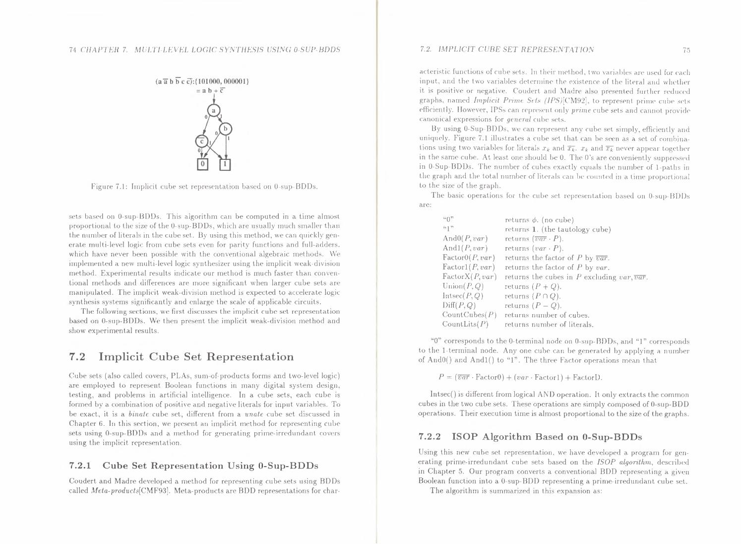
74 CHAPTER 7. MULTI-LEVEL LOGIC SYNTHESIS USING 0-SUP-BDDS

(a ab b c C):{lOlOOO, 000001} =ab+c

Figure 7.1: Implicit cube set representation based on 0-sup-BDDs.

sets based on 0-sup-BDDs. This algorithm can be computed in a time almost proportional to the size of the 0-sup-BDDs, which are usually much smaller than the number of literals in the cube set. By using this method, we can quickly gen­erate multi-level logic from cube sets even for parity functions and full-adders. which have never been possible with the conventional algebraic methods. We implemented a new multi-level logic synthesizer using the implicit weak-division method. Experimental results indicate our method is much faster than conven­tional methods and differences are more significant when larger cube sets are manipulated. The implicit weak-division method is expected to accelerate logic synthesis systems significantly and enlarge the scale of applicable circuits.

The following sections, we first discusses the implicit cube set representation based on 0-sup-BDDs. We then present the implicit weak-division method and show experimental results.

7.2 Implicit Cube Set Representation

Cube sets (also called covers, PLAs, sum-of-products forms and two-level logic) are employed to represent Boolean functions in many digital system design, testing, and problems in artificial intelligence. In a cube sets, each cube is formed by a combination of positive and negative literals for input variables. To be exact, it is a binate cube set, different from a unate cube set discussed in Chapter 6. In this section, we present an implicit method for representing cube sets using 0-sup-BDDs and a method for generating prime-irredundant covers using the implicit representation.

7.2 .1 Cube Set Representation Using 0-Sup-BDDs

Coudert and Madre developed a method for representing cube sets using BDDs called Meta-products(CMF93]. Meta-products are BDD representations for char-

7.2. IMPLICIT CUBE SET REPRESENTATION 75

acteristic functions of cube sets. In their met hod, two variables are used for C'ach input, and the two variables determine the existence of the literal and whether it is positive or negative. Coudert and Madre also presented further reduced graphs, named Implicit Prime Sets (JPS)[CM92], to represent prime cube sds efficiently. However, IPSs can represent only prime cube sets and cannot provide canonical expressions for geneml cube sets.

By using 0-Sup-BDDs, we can represent any cube set simply, efficiently and uniquely. Figure 7.1 illustrates a cube set that can be seen as a set of combina­tions using two variables for literals Xk and Xk· Xk and Xk never app{'ar tog<'tlwr in the same cube. At least one should be 0. The O's are conveniently suppress<'d in 0-Sup-BDDs. The number of cubes exactly equals the number of 1-paths in the graph and the total number of literals can be counted in a time proportional to the size of the graph.

The basic operations for the cube set representation based on 0-sup-BDDs are:

"0" "1" AndO(P, var) Andl ( P, var) FactorO( P, var) Factor 1 ( P, var) FactorX(P, var) Union(P,Q) Intsec(P, Q) Diff(P,Q) CountCubes(P) CountLits(P)

returns</>. (no cube) returns 1. (the tautology cube) returns ( var · P). returns ( var · P). returns the factor of P by var. returns the factor of P by var. returns the cubes in P excluding var, var. returns (P + Q). returns (P n Q). returns (P- Q). returns number of cubes. returns number of literals.

"0" corresponds to the 0-terminal node on 0-sup-BODs, and "1" corresponds to the !-terminal node. Any one cube can be generated by applying a number of AndO() and Andl() to "1". The three Factor operations mean that

P = ( var · FactorO) + (var · Factorl) + FactorO.

lntsec() is different from logical AND operation. It only extracts the common cubes in the two cube sets. These operations are simply composed of 0-sup-800 operations. Their execution time is almost proportional to the size of the graphs.

7.2.2 ISOP Algorithm Based on 0-Sup-BDDs

Using this new cube set representation, we have developed a program for gen­erating prime-irredundant cube sets based on the !SOP algorithm, described in Chapter 5. Our program converts a conventional BDD representing a given Boolean function into a 0-sup-BDD representing a prime-irredundant cube set.

The algorithm is summarized in this expansion as:

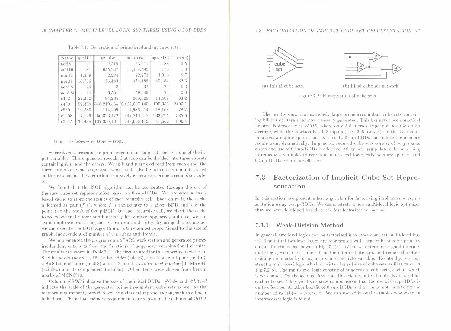
76 CJIAPTEH 7. MUl-TI-LEVEL LOGIC SY:VTJJE8IS t'SI.\G 0-S{;P-BDDS

Table 7.1: Generation of primc-irrcdundant cube sets.

Name #BDD #Cube #Literal #ZBDD Time(s)

add8 41 2,519 23,211 88 0.5 add16 81 655,287 11 ,.168,59.5 176 1.3 rnult6 1,358 2,284 22,273 3,31.5 5.7

rnult8 10,766 3.5,483 474,488 45,484 82.3 achil8 24 8 32 24 0.3

achil8n 24 6,561 59,049 24 0 .3

C'132 27,302 84,235 969,028 14,407 83.2 c499 52,369 fJ48,219,564 ~.462,057 ,445 195,356 2400.1 c880 19,580 114,299 1,986,01'1 18,108 78.7

c1908 17,129 56,323,472 1,6'17,240,617 233,775 385.6 c5315 32,488 137,336,131 742,606,419 41,662 886.4

isop = v · 1sop0 + v · isop1 + isopd

wherc i.-;op rcpresents the prime-irredundant cube sct, and v is one of the in­put variablcs. This expansion reveals that 1sop can be divided into three subsets containing v, u, and the others. When v and 1' arC' excluded from each cube, the thrC'c subsets of isoph isop0 and isopd should also be prime-irredundant. Based 011 this <'Xpansion, the algorithm r<'cursively generates a primc-irredundant cube set.

Wc found that the ISOP algorithm can be accclcrakd through the use of the new cube set representation based on 0-sup- BDOs. We prepared a hash­based c·ache to store the results of each rccursiv<' call. Each entry in the cache is formed as pair {!, s ), where f is the pointer to a given BOO and s is the pointer to the result of 0-sup-BOO. On each recursive call, we check the cache to se<' whether the same sub-function f ha<> al ready appeared, and if so, we can avoid duplicate processing and return result ~ directly. By using this technique, wc can cxccute the ISOP algorithm in a time almost proportional to the size of graph, indcpendent of number of the cubes and literals.

We implemented the program on a SPA RC work station and generated prime­irredundant cube sets from the functions of large-scale combinational circuits. The results an• shown in Table 7.1. The circuits uscd fort his exp<'rimcnt were: an 8+8 bit adder (add8), a 16+16 bit adder (addl6), a 6x6 bit multiplier (mult6), a 8x8 bit multiplier (mult8) and a 21-input Achzllc.·i hc.el function{BH~1SV84] (achil8p) and its complement (achil8n). Other items were chosen from bench­marks of MCNC"90.

Column #ROD indicates th<:' size of the initial BDDs. #Cube and #Litem! indicate t h(• scale of the generated prim<' irredundant cube sets as well as tlw memory requirement, provided we use a classical representation, such as a linear link<'d list. The actual memory r<'quircments arc shown in the column #ZBDD.

(a) Initial cube sets. (h) Final cube set network.

Figure 7.2: Factorir,ation of cube sets.

The results show that extremely large prinu:-irredundant cube sets contain­ing billions of literals can now be easily gcnerat<•d. This has never been pract.ical before. Noteworthy is cS.'JJS, wht'r<' only 5.5 literals appear in a cube on an average, while the function has 178 inputs (i. <'., :356 literals). In this ca-;e corn­binations are quite sparse, and as a result, 0-sup BDDs can reduce the memory requirement dramatically. In general, rf'dured cube' sets consist of very spars<' cubes and use of 0-Sup-BODs is cffc•ctive. \\'hc•n we manipulate cube' sds using intermediate variables to represent multi l<•vcl logic, cube sets arc• sparser. and 0-Sup-BDDs even more effective.

7.3 Factorization of Implicit Cube Set R epre­sentation

In this section, we present a fast algorithm for factorizing implicit rub<' r<·prc

sentat ion using 0-sup-BODs. \Ve demonstrate a new multi-level logic oplimi7.f't t.hat we have developed based 011 thc fast factorization method.

7.3.1 Weak-Division M ethod

In generaL two-level logics can be factoritcd into more compact multi-level log ics. The initial two-level logic.<; arc repn•sented with large cube sets for primal) output functions, as shown in Fig. 7.2(a). Wh<·n we detC'rminc a good int<·nnc·­diate logic. we make a cube s<'t for thC' intC'rnwcliat~ logic and reduc<' the otlwr cxisting cube sets by using a n<>w intermN!iate variable. EvC'ntually, we con­struct a multi-level logic which consists of small size of cube sets as illustrat<·d in Fig 7.2(b). The multi-level logic consists of hundreds of cube sets, each of which is vcry small. On th<" average. IC'ss t.han 10 variable's out of hundreds are used for each cube set. They yield so spars(• combinations that the u<;e of 0-sup-BDDs is quite effective. Another ben<>fit of 0-sup BDDs is that W<' do not have to fix lh<' number of variables beforehand. W(' can use additional variables whenever an

int.crmediate logic is found.

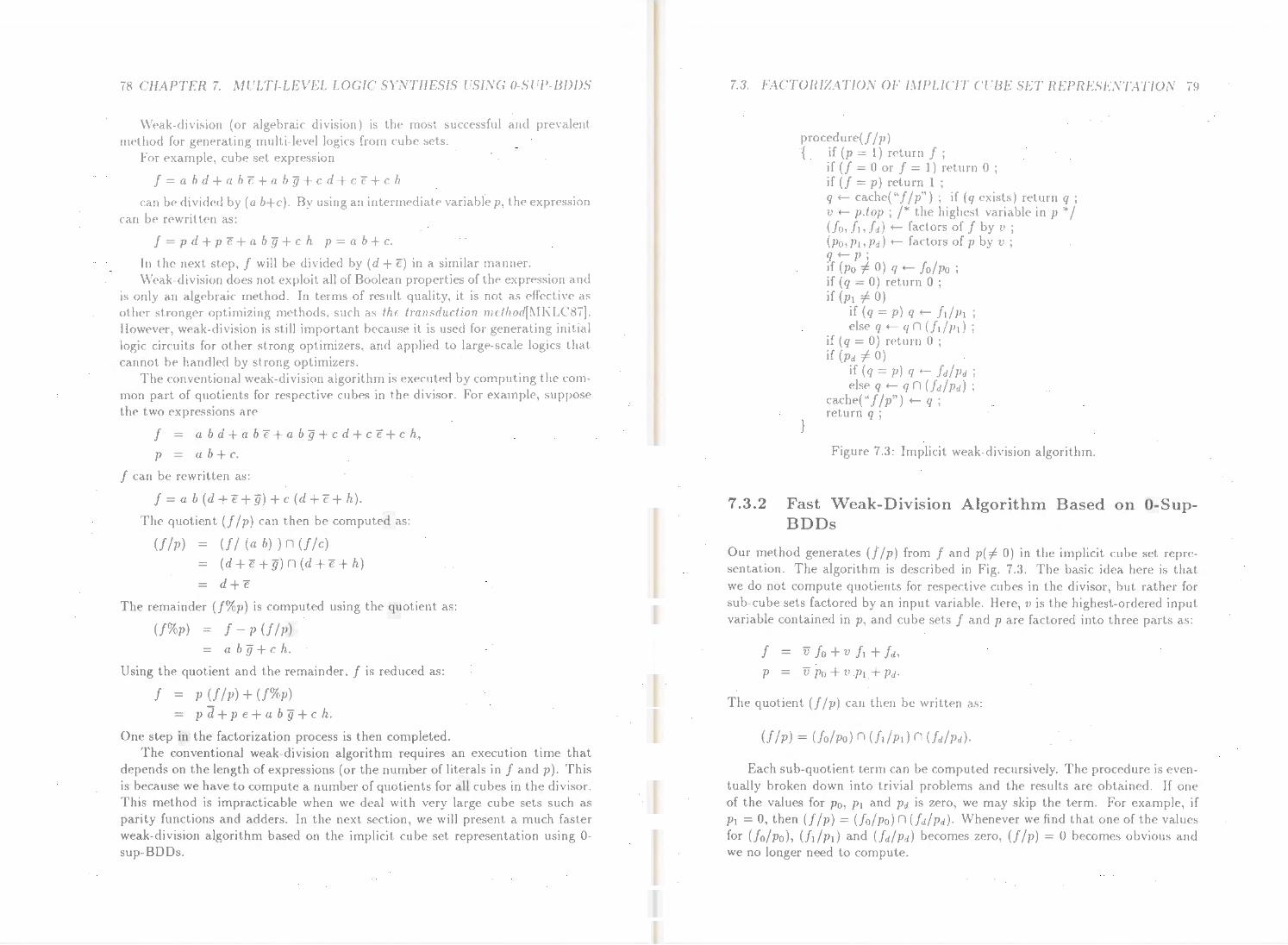
78 CHAPTER 7. MlrLTI-LEVEL LOGIC SY,\JTHESIS USING 0-St'P-BDDS

Weak-division (or algebraic division) is the most successful and prevalent mf'thod for generating multi-level logics from cube sets.

For example, cube set expression

f=abd+abe+abg+cd+cc+ch

can be divided by (a b+c). By using an intermediate variable p, the expression can be rewritten as:

.f = p d + p e + a b 9 + c h p = a b + c.

rn the next step, f will be divided by (d +e) in a similar manner. Weak-division does not exploit all of Boolean properties of the expression and

is only an algebraic method. In terms of result quality, it is not as effective as other stronger optimizing methods, such as the tmnsduclion melhod[~1KLC87]. Howev<'r, weak-division is still important because it is used for generating initial logic circuits for other strong optimizcrs, and applied to large-scale logics that cannot bf' handled by strong optimizers.

The conventional weak-division algorithm is executed by computing the com­mon part of quotients for respective cubes in the divisor. For example, suppose the two expressions are

f = a b d + a b e + a b 9 + c d + c e + c h, p = ab+ c.

f can be rewritten as:

f = a b ( d + e + g) + c ( d + e + h).

The quotient (! fp) can then be computed as:

UIP) - U/ (a b)) n (fie) = (d + e +g) n (d + e +h)

= d+e

The remainder (J%p) is computed using the quotient as:

(J%p) = f - P U I P) = ab g + c h.

Using the quotient and the remainder, f is reduced as:

f = p UIP) + (f%p) = p d + p e + a b g + c h.

One step in the factorization process is then completed. The conventional weak-division algorithm requires an execution time that

depends on the length of expressions (or the number of literals in f and p). This is because we have to compute a number of quotients for all cubes in the divisor. This method is impracticable when we deal with very large cube sets such as parity functions and adders. In the next section, we will present a much faster weak-division algorithm based on the implicit cube set representation using 0-sup-BDDs.

7.3. FACTORIZATION OF L\fPLICIT CCBE SET REPRESENTATION 79

procedure(! lP) { if (p = 1) return f ;

}

if (! = 0 or f = 1) return 0 ; if(!= p) return l ; q +--cache("! lP"); if (q exists) return q; v +-- p.top ; I* the highest variable in p *I (Jo, /1, /d) +-- factors of f by v ; (po, Pt, Pd) +-- factors of p by v ; q +-- p; if (Po =1- 0) q +-- foiPo ; if (q = 0) return 0 ; if (Pt =/:- 0)

if ( q = p) q +-- !J I PI ; else q +-- q n Ut!Pt) ;

if (q = 0) return 0 ; if (Pd =/:- 0)

if (q = p) q +-- .fdiPd ; else q +-- q n UdiPd) ;

cache("/ fp") +-- q ; return q ;

Figure 7.3: Implicit weak-division algorithm.

7.3.2 Fast Weak-Division Algorithm Based on 0-Sup­BDDs

Our method generates (.ffp) from f and p(f- 0) in the implicit cube set repre­sentation. The algorithm is described in Fig. 7.3. The basic idea here is that we do not compute quotients for respective cubes in the divisor, but rather for sub-cube sets factored by an input variable. Here, v is the highest-ordered input variable contained in p, and cube sets f and p are factored into th ree parts as:

f p - v Po + v P1 + Pd·

The quotient (! fp) can then be written as:

Each sub-quotient term can be computed recursively. The procedure is even­tually broken down into trivial problems and the results are obtained. If one of the values for p0 , p1 and Pd is zero, we may skip the term. For example, if Pt = 0, then (.f lP) = UoiPo) n (.fdiPd)· Whenever we find that one of the values for UoiPo), (Jtfp1) and (Jd/Pd) becomes zero, (J lP) = 0 becomes obvious and we no longer need to compute.

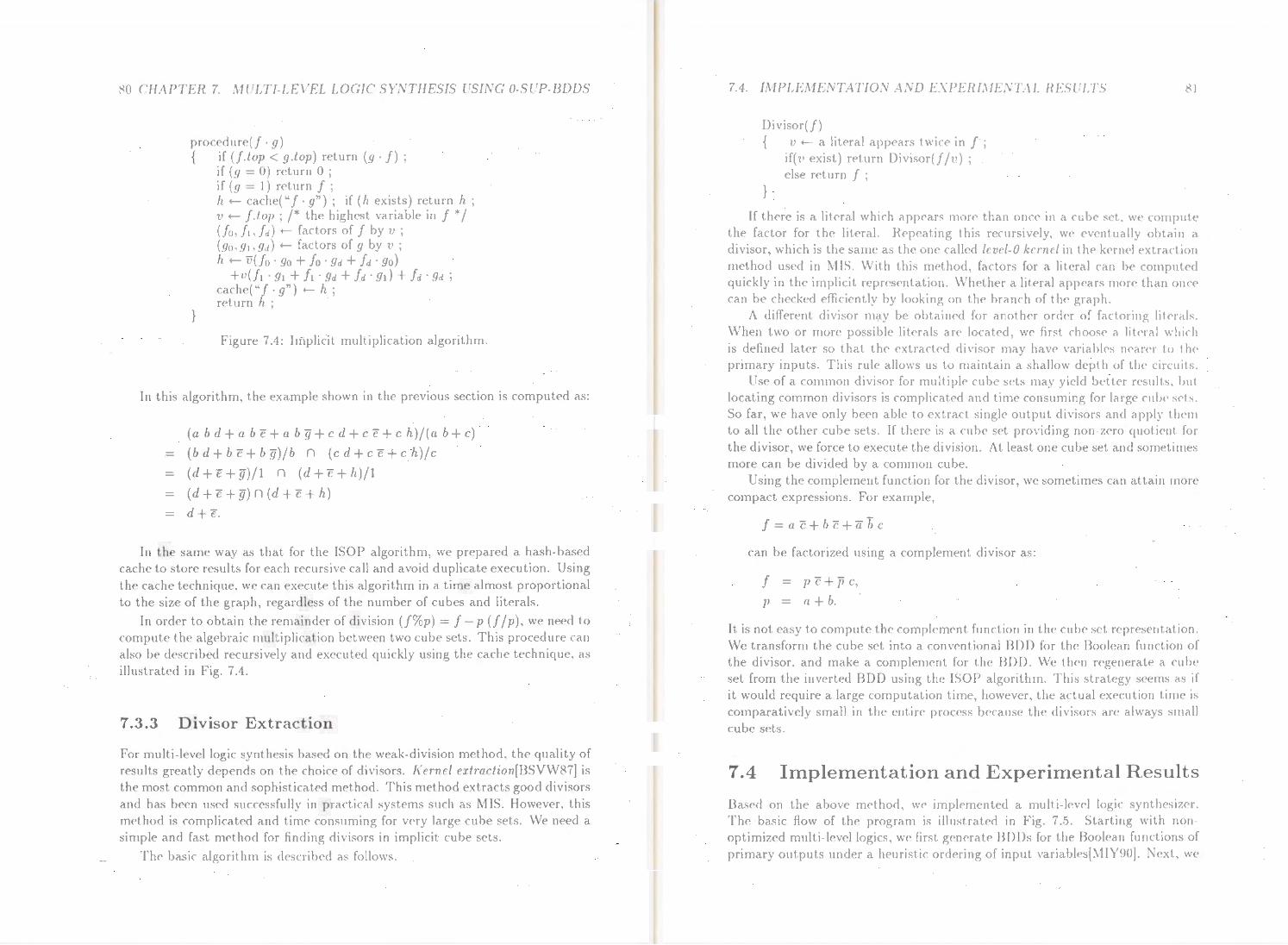
80 CHAPTER 7. MULTI-LEVEL LOGTC' SYNTHESIS USING 0-SUP-BDDS

proced ure(J · 9) { if (f.top < 9.top) return (g ·f) ;

if (9 = 0) return 0 ;

}

if (g = 1) return f; h- cache("!· 9") ; if (h exists) return h ; v - f. top ; I* the highest variable in f *I (Jo, /t, /d) - factors of f by v ; (go, 9t, 9d) - factors of g by v ; h - v(Jo 0 9o + !o 0 9d + !d 0 9o)

+v(JJ · 9t + ft · 9d + !d · 91) + !d · 9d ; cache("!· g") - h ; return h ;

Figure 7.4: Implicit multiplication algorithm.

In this algorithm, the example shown in the previous section is computed as:

(ab d +ab e +ab g + c d + c e + c h)l(a b +c) ( b d + b e + b g) 1 b n ( c d + c e + c h) 1 c

(d+e+g)l1 n (d+e+h)l1

- ( d + e + g) n ( d + e + h) - d+e.

In the same way as that for the ISOP algorithm, we prepared a hash-based cache to store results for each recursive call and avoid duplicate execution. Using the cache technique, we can execute this algorithm in a time almost proportional to the size of the graph, regardless of the number of cubes and literals.

In order to obtain the remainder of division (f%p) = f- p (f lp), we need to compute the algebraic multiplication between two cube sets. This procedure can also be described recursivcly and executed quickly using the cache technique, as illustrated in Fig. 7.4.

7 .3.3 Divisor Extraction

For multi-level logic synthesis based on the weak-division method, the quality of results greatly depends on the choice of divisors. [{erne/ extraction(BSVW87] is the most common and sophisticated method. This method extracts good divisors and has been used successfully in practical systems such as MIS. However, this method is complicated and time consuming for very large cube sets. We need a simple and fast method for finding divisors in implicit cube sets.

The basic algorithm is described as follows.

7.4. L\JPLEMENTATJON ASD EXPERl.\lESTt\L RESULTS

Divisor(!) { v - a literal appears twice in f ;

}

if(v exist) return Divisor(flv); else return J ;

81

If there is a literal which appears more than once in a cube set, we compute the factor for the literal. Repeating this recursively, we eventually obtain a divisor, which is the same as the one called level-0 kernel in the kernel extraction method used in MIS. With this method, factors for a literal can be comput<'d quickly in the implicit representation. Whether a literal appears morC' than onc<' can be checked efficiently by looking on the branch of the graph.

A different divisor may be obtained for another order of factoring litNals. When two or more possible literals are located, we first choose a lit<'l"al which is defined later so that the extractC'd divisor may have variables nC'arN to t lw primary inputs. This rule allows us to maintain a shallow depth of tlw circuits.

Use of a common divisor for multiple cube sets may yield bctt<'r r<'sults, but locating common divisors is complicated and time consuming for large cui)(' SC'ts. So far, we have only been able to extract single output divisors and apply them to all the other cube sets. If there is a cube set providing non-z<'ro quotient for the divisor, we force to execute the division. At least one cube set and sometimes more can be divided by a common cube.

Using the complement function for the divisor, we sometimes can attain more compact expressions. For example,

can be factorized using a complement divisor as:

J - pc+ pc, p - a+ b.

It is not easy to compute the complement function in the cube set representation. We transform the cube set into a conventional BDD for the Boolean function of the divisor, and make a complement for t.he BOO. We then regenerate a cube set from the inverted BOO using the !SOP algorithm. This strategy s<>ems as if it would require a large computation time, however, the actual execution time is comparatively small in the entire process b<>cause the divisors ar<' always small cube sets.

7.4 Imple m e ntation and Expe rimental R esults

Based on the above method, w<> implemented a multi-level logic synthesizer. The basic flow of the program is illustrated in Fig. 7 .. 5. Starting with non­optimized multi-level logics, we first g<-'nC'rat<" BDDs for the Boolean functions of primary outputs under a heuristic ordering of input variables(~11Y90]. Next, we

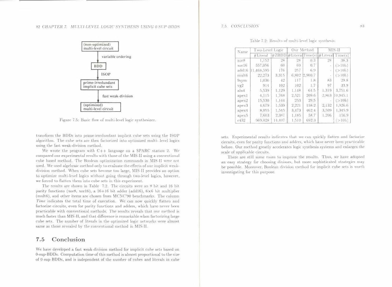
82 CHAPTER 7 . . \fULTI-LEVEL LOGIC SY.\"THESIS l S/.\G 0 Sl P-BDDS

(non-optimized) multi-level circuit

variable or de ring

I BOO I ISOP

prime-irredundant implicit cube sets

fast weak-division

(optimized) I multi-level ci rcuit

Figure 7.5: Basic flow of multi-level logic syntlwsizer.

transform the BDDs into prime irredundant implicit cube sets using the ISOP algorithm. TIH' cube sets are then factorized into optimized multi- level logics using the fa!-it weak-division method.

We wrote th<' program with C++ language on a SPARC station 2. \\'e compared our experimental results with those of the ~1IS-ll using a conventional cube based method. The Boolean optimization commands in MIS-II were not used. We used algebraic method only to evaluate the effects of our implicit weak­division mct.hod. When cube sets become too large, MIS-II provides an option to optimizC' multi lc•vel logics without going through two-level logics, however, we forced to flatten them into cube ~C'ts in this experiment.

The results arc shown in Table 7.2. The circuits were an 8 bit and 16 bit parity functions (xor8, xor16). a 16+16 bit adder (add16) , 6x6 bit multiplier (mult6), and other items are chosen from MC~C'90 benchmarks. The column Time indicates the total time of execution. \Ve can now quickly flatten and factorize circuits, even for parity functions and adders, which have never been practicablE' with conventional methods. T'he results reveals that our method is much faster than MIS IT , and that difference is remarkable when factorizing large cube sets. The number of literals in the optimized logic net.,vorks were almost same as thost> revealed by the conventional method in MIS 11.

7.5 Conclusion

We have developed a fast weak-division method for implicit cube sets based on 0-sup-BDDs. Computation time of this method is almost proportional to the size of 0-sup-BDDs, and is independent of the number of cubes and literals in cube

7 . .s. eo.\ cu.:sros

Table 7.2: Hcsults of multi-levd logic syntlwsis.

Name Two- Level Logic Our ~1ethod ~11S-ll

#Literal #ZBDD #Litera Tinw(s) # Lit<·ra Time(s) xor8 1,152 28 28 o.:3 ~8 38.:3 xorl6 557.056 60 60 0.7 - ( > 1 Oh) addl6 11,468.595 176 •)--_;)I 6.9 - (> lOh) rnult6 22,273 :3) 1 ') 6,802 ~.900.7 (>I Oh) 9sym 1,036 '12 117 1.8 83 29.8 vg2 914 102 102 1.7 97 33.9 alu4 5,.539 1.129 1 '148 6'1.5 1,319 3.751.6 apex1 4,11.5 1,768 2,521 209.6 2,863 I 0,94.5.1 apex2 15,530 1.1'1·1 253 29.5 - ( > 1 Oh) apex3 4.679 1.5:39 2,221 158.2 2,132 1,926.6 apex4 8,055 1,51.') 3,473 462.1 3,509 1,345.9 apex.5 7,603 2,387 1.185 58.7 1,206 156.9 c432 969,028 11,407 1 ,.510 692.:3 (>10h)

sets. Experimental results indicates that we can quickly flatten and factoriz<' circuits, even for parity functions and adders. which have' never been practicC\h\(• before. Our method greatly accelerates logic synthesis systems and enlarges the scale of applicable circuits.

There are still some room to improve the results. Thus, we have adoptc·cl an easy strategy for choosing divisors, but more sophistical<'d strategi<'s rnay be possible. Moreover, Boolean division method for implicit cube sets is worth investigating for this purpose.

84 CHAPTER 7. MULTI-LEVEL LOGIC SYNTHESIS USING 0-SUP-BDDS

Chapter 8

Arithmetic Boolean Expressions

8.1 Introduction

In the research and development of digital systems, Boolean expressions arc sometimes used to handle problems and procedures. It is a cumbersome job to calculate Boolean expressions by hand, even if they have only a few variables. If they have more than five or six variables, we might as well give up. This prob­lem motivated us to develop a Boolean Expression Manipulator (BEM)[MJY89], which is an interpreter that uses BDDs to calculate Boolean expressions. It en­ables us to check the equivalence and implications of Boolcan expressions quite easily. It has helped us in developing VLSI design systems and solving combi­natorial problems.

Although most discrete problems can be described by Boolean expressions, arithmetic operators, such as addition, subtraction, multiplication and compari­son, are convenient for describing many practical problems, as seen in 0-J linear programming. Such expressions can be rewritten using logic operators only, but this can make them complicated and hard to read. In many cases, arithmetic operators provide simple problem descriptions of problems.

In this chapter, we present a new Boolean Expression Manipulator, which we

call BEM-11, that allows the use of arithmetic operators. DEM-II can dir('ctly solve problems represented by a set of equalities and inequalities , which arc d('alt with in 0-1 linear programming. Of course, it can also manipulate ordinary Boolean expressions as well. We developed several output formats for displaying expressions containing arithmetic operators.

In the following sections, we first show a method for manipulating Boolean expressions with arithmetic operations. We then present implementation of the arithmetic Boolean expression manipulator and its applications.

8.5

86 CHAPTER 8. AHTTII.\IE'l'IC JJOOU~ \.\' EXPHESSJ0.\5

8.2 Manipulation of Arithmetic Boolean Ex-.

preSSIOnS

As W«' disc:usscd above. although most discrete problems can be d<'sc:ribed by using Boolc•an expressions. arithnwtic operators are useful for desc:ribing many prac:t ical problems. For example. a majority function with five inputs can be <'xpre'isC'd concisely by using arithmetic op<•rators

Using only Boolcan expressions, this function b<·come complicated as:

(.r 1 1\ x 2 1\ x 3 ) V (x 1 1\ x21\ x4) V (x, 1\ .r2 1\ .rs) V(.r, 1\ .X3/\ X4) V (Xt 1\ X31\ .rs) V (.rt 1\ .r, 1\ Xs)

V(.r 2 1\ x 3 1\ X4) V (x2 1\ x 3 1\ X.c;) V (.r2 1\ X4 1\ Xs) V(.ra 1\ X4 1\ xs).

In this scc:tion. we describe an efficient method that uscs BOOs to represent and manipulate c>xpressions with arithmetic oprrators.

8.2 .1 Definitions

For manipulating Boolean expressions that includc arithmetic operators. we de­fill<' ar·ithmctir Boolean expressions and Boolcan-to-mtcgcr functions, which are cxtcndcd models of conventional Boolean expressions and Boolean functions.

Definition 8.1 Arithmetic Boolean expressions arc extended Boolean ex-7Jrcssions which contain not only logic opemt o1·s, but also m·ithmelic operato1·s, .cmch as addition(+), subtraction(-), and multiplication (x). Any integer num­bc7' lS allowed to be used as a constant term in the expression, btd input variables a1·c 7Y'Stnclcd to either 0 or 1. Equality(=) and inequalities {<, >, ~. 2:, =/=) are defined as operations which return a value of either I (t1·ue) or 0 (false).

For example, (3 x x 1 + x 2 ) is an arithmetic Boolean expression with respect to the variables x 1 , .r2 E { 0, 1}. (3 x x 1 + x2 < 4) is another example.

When ordinary logic operations are applied to integer values other than 0 and 1, we define them as bit-wise logic operations for binary-coded numbers, like in many programming languages. For example, (3 V 5) returns 7. Vnder this modcling scheme, conventional Bool<'an expressions become special cases of

arithmetic Boolcan functions. The value of thc expression (3 x x 1 + .r2) becomes 0 when x, = x2 = 0,

or 4 when x 1 = x2 = 1. \Ve can see that an arithmetic Boolean expression represents a function from binary-vector to integer: ( 8 11

-t I). \"'e call this function a Boolean-to-integer (B-to-I) function , which has been discussed in Section 4.2. The operators in arithmetic 13oolcan expressions are defined as operations on B-to-1 functions. We can calculate B-to-1 functions for arithmetic

8.2. MANIPULATIOX OF ARITJ/.\IETIC HOOUj. \\ EXPRESSIO.\S 87

.r., :l' •l 00 Ol 10 11

3 X Xt 0 0 3 3 3 X Xt + I2 0 3 4 3 X It + X2 < 4 0

Figure 8.1: Computation of arithmetic Boolcan expressions.

(f3) t2 n ro B-to-1 function

xt x2 r (t2 n to> 0 0 0 (0 0 0) 0 1 J (0 0 1) •

0 3 (0 I I ) 4 (1 0 0)

(a) A MTBDD. (b) A BDD vector.

Figure 8.2: Representation for B-to-1 functions.

Boolean expressions by applying operations on B-to-1 functions according to the structure of the expressions.

The procedure for obtaining the B-to-1 function for the expression (3 x x 1 + x2 < 4) is shown in Fig. 8.1. First, multiply tlw constant function 3 times input function x 1 to obtain the B-to-1 function for (3 x xt). Then add x2 to obtain the function for (3 x x1 + x 2 ). Finally we can get a B-to-1 function for th<' entire expression (3 x x 1 + x2 < 4) by applying the comparison operator ( <) to the constant function 4. \Ve find that this arithmetic Boolean expression 1s

equivalent to the expression (XI V x 2 ).

8.2.2 Representation of B-to-1 Functions

Figure 8.1 showed how a B-to-1 function can he obtained by enumerating th<· output values for all possible combinations of the input values. This is impracti cal when there are many input variables sincc the number of combinations grows exponentially. We thus need a more efficient way to represent B-to- 1 functions.

As discussed in Section 4.2, there are two ways to represent B-to-1 functions using BDDs: multi-terminal BDDs (MTBDDs) and BDD vectors. MTBDDs are extended BDDs with multiple terminals, each of which has an integer valu<' (Fig. 8.2(a)). BDD vectors are the way to represent B-to- I functions with anum­ber of BDDs by encoding the integer numbers into binary vectors (Fig. 8.2(b)).

88 CHAPTER 8. ARITJ/METIC 1300U~AN EXPRESS/0.\'S

F 100 F

Figure 8.3: BOO vectors for arithmetic Boolean expressions.

F 2F 3F 100 F

Figure 8.4: MTBDDs for arithmetic Boolean expressions.

The effici<'ncy of the two representations depends on the nature of the objec­tive functions. In manipulating arithnwtic Boolean expressions, we often gener­ate B to I functions from Boolean functions, as when we calculate F x 2, F x 5, or F x 100 from a certain Boolean function F. In such cases, the BDD vectors can be conveniently shared with each other ( Fig. 8.3). However, multi-terminal HODs cannot be shared (Fig. 8.4). \\'<' therefore use BDD vectors for manipu­lating arithmetic Boo lean expressions.

For negative numbers, we use 2's complement representation in our imple­mental ion. The most significant bit is used for the sign bit, whose BDD indicates und<'r which conditions the B-to-1 function produc<'s a negative value. This en­coding scheme requires fixing the bit length in advance, and it limits the range of ntunb<'rs. We allocate a sufficiently long bit length to avoid inconvenience from this constraint.

8.2. MA.I\'IPULA.TIOS OF .AHJTJIME'l'JC /lOOI.F \.\ EXPRESSIO\'S

3 n n ro

~lb • times

x1 n n ro / Jn

4 n n ro

Jb

• less

7

3 xl + x2 < 4 n n ro

Figure 8.5: Generation of BDD V<'dors for arithm<'tic Boolean expressions.

8 .2.3 Handling B-to-I functions

89

This section explains how to handle B-to l functions represented by BOD vectors.

Logic operations, such as AND, OR, and EXOR, are implemented as bit~ wise operations between two BDD vectors. Applying BDD operations to their respective bits, a new B-to-1 function is g<'neratcd. We define two kinds of inversion operations: bit-wise inversion and logical inv<>rsion. Logical inversion returns 1 only for 0, otherwise it returns 0.

Arithmetic addition can be composed using logic operations on BOOs by simulating a conventional hardware algorithm of full adders which are designed as combinational circu.its. We use> a simpl<· algorithm for a ripple carry adder, which computes from the lower bit to th<' high<'r bit, propagating carri<>s. Other arithmetic operations, such as subtract ion, multiplication, division and shifting can be composed in the same way. Exception handling should b<> considered for overflow and division by zero.

Positive/negative checking is immC'diat<•ly indicated by the sign-bit BDD. Using subtraction and sign checking. we can compose comparison operations between two B-to-1 functions. TheM' operations gerl<'ral<' a new 8-to-I function that returns a value of either l or 0 to CXJ>r<'SS wheth<'r the equality or inequality is satisfied.

It is useful if we can find the uppc•r (or low<'r) bound value of a B-to-1 function for all possible combinations of input valuC's. This can be done cfflciently by using binary search. To find the uppcr bound, we• first ch<>ck whether the function can <'V<'r <>xceed 2". If thcre is a casf' in which it does, we th<'n compare it with 2" + 2"- 1

, otherwise with only 2"- 1. ln this way, all the bits can be determined

from the highest to the lowest, and eventually t h<' upp<'r bound is obtained. The• lower bound is found in the same way.

90 CHAPTER 8. ARITJ-L\tfETIC BOOLEAN EXPRESSIOt\'5

f=2a+3b-4c+d

• •• cd ab·... 00 01 11 10 .

00

01

11

10

0

3

5

2

1

4

6

3

-3 -4

0 -1

2 1

-1 -2

Figure 8.6: An integer Karnaugh map.

Computing the upper (or lower) bound is a unary operation for B-to-1 func­tions; it returns a constant B-to-1 function and can be used conv<'niently in arithmetic Boolean expressions. For example, the expression:

UpperBound(F) == F (F is an arithmetic Boolean expression)

gives a function which returns 1 for the inputs that maximize F, otherwise it returns 0. Namely it computes the condition for maximizing F.

An example of calculating arithmetic Boolean expressions using BDD vectors

is shown in Fig. 8.5.

8.2.4 Display Formats for B-to-I Functions

We propose several formats for displaying B-to-I functions represented by BOOs.

Integer K a rna ugh m ap s

A conventional Karnaugh map displays a Boolean function using a matrix of logic values (0, 1 ). We extended the Karnaugh map to use integer numbers for each element (F ig. 8.6). We call t.his an integer Karnaugh map. It is useful for observing the behavior of B-to-I functions. Like ordinary Karnaugh maps, they are practical only for fewer than five or six input functions. For a larger number of inputs, we can make an integer Karnaugh map with respect to only six input variables, by displaying the upper (or lower) bound for the rest of variables on each element of the map.

Bit-wise expressions

When the objective function is too complicated for an integer Karnaugh map, the function can be d isplayed by listing Boolean expressions for respective bits of the B DD vector in the sum-of-products format. F igure 8.7 shows a bit-wise expression for the same function shown in Fig .8.6. We used the ISO P algorithm,

8.2. MANIPULATIO.V OF AR!Tfl.\JETIC DOOLEAX E.\PRESSIO.VS

f=2xa+3xb-4xc+d

(a" c" d) v (b" c) (a 1\ b 1\ c) v (a 1\ c 1\ d) v ( b 1\ c 1\ d) v (b 1\ c)

(a 1\ b) V (a 1\ d) V (a 1\ b 1\ d) ( b 1\ d) V (b 1\ d)

Figure 8.7: A bit-wise expression

6 a/\b/\c/\d 5

4

3

2

1

0

-1

-2 -3

-4

a/\b/\c/\d a/\b/\c/\d (a 1\ b 1\ c 1\ d) v (a 1\ b 1\ c 1\ d) (a 1\ b 1\ c 1\ d) V (a 1\ b 1\ c 1\ d) (a 1\ b 1\ c 1\ d) v (a 1\ b 1\ c 1\ d)

(a 1\ b " c " d) v (a 1\ b 1\ c 1\ d) (a 1\ b 1\ c 1\ d) v (a 1\ b 1\ c 1\ d) a/\b/\c/\d

a/\b/\c/\d

a/\b/\c/\d

Figure 8.8: Case enumeration format.

91

which has been described in Chapter 5, to generate a compact sum-of-products format on each bit. Bit-wise expression is not so helpful for showing the behavior of B-to-I functions, but it does allow us to observe the appearance frequency of an input variable and it can estimate a kind of complexity of the functions. If a function never has negative values, we can suppress the expression for the sign bit. If some higher bits are always zero, we can omit showing them. With this zero suppression, a bit-wise expression becomes a simple Boolcan expression if the function returns only 1 or 0.

Case enumeration

Using case enumeration, we can list all possible values o f a function and display the condition fo r each case using a sum-of-products format (Fig. 8.8). This format is effective when there are many input variables but the range of output values is limited .

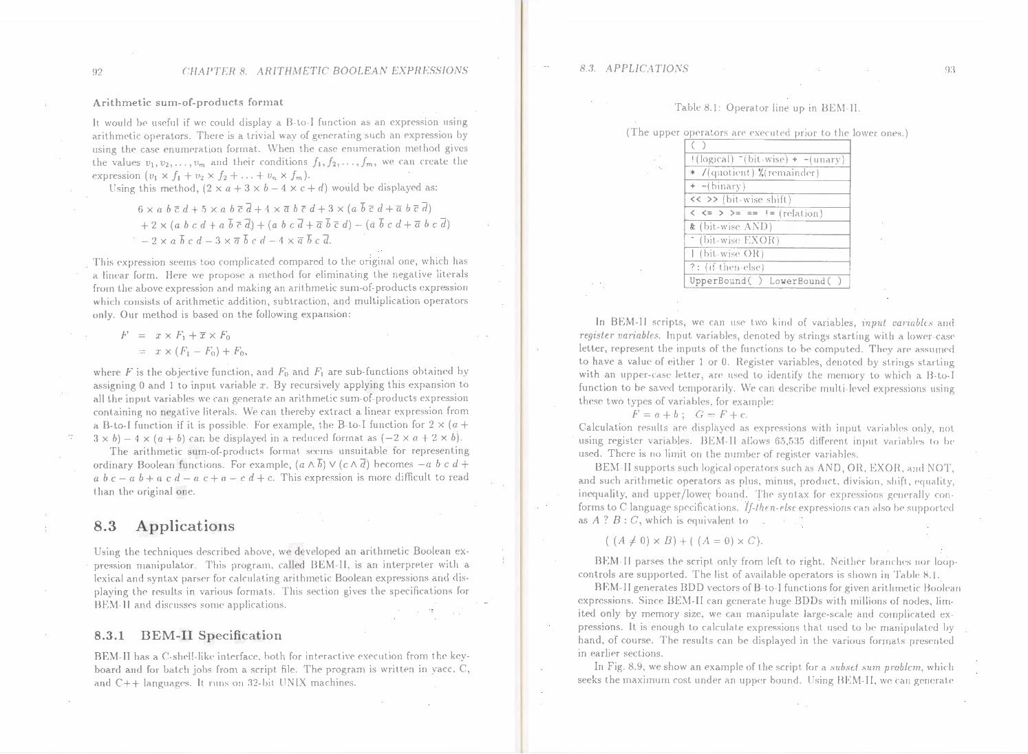
92 CHAPTER 8. ARITHMETIC BOOLEAN EXPRESSIONS

Arithmetic sum-of-products format

It would be useful if we could display a B-to-1 function as an expression using arithmetic operators. There is a trivial way of generating such an expression by using thC' case enumeration format. When the case enumeration method gives the values v1, v2 , ••. , Vm and their conditions j 1 , h, ... , fm, we can create the expression (vt X !1 + v2 X !2 + ... + Vn X fm)·

Using this method, (2 x a+ 3 x b- 4 x c +d) would be displayed as:

6 x a b c d + 5 x a b c d. + 4 x a b c d + 3 x (a b c d + a b c d)

+ 2 x (a b c d + a b c d) + (a b c d. + a b c d) - (a b c d + a b c d)

-2xabcd-3xabcd-4xabcd.

This expression seems too complicated compared to the original one, which has a linear form. Here we propose a method for eliminating the negative literals from the above expression and making an arithmetic sum-of-products expression which consists of arithmetic addition, subtraction, and multiplication operators only. Our method is based on the following expansion:

F - x x F1 + x x Fo

x x ( F1 - Fo) + Fo,

where F is the objective function, and F0 and F1 are sub-functions obtained by assigning 0 and 1 to input variable x. By recursively applying this expansion to all the input variables we ran generate an arithmetic sum-of-products expression containing no negative literals. We can thereby extract a linear expression from a B-to-1 function if it is possible. For example, the B-to-1 function for 2 x (a+ 3 x b)- 4 x (a+ b) can be displayed in a reduced format as ( -2 x a+ 2 x b).

The arithmetic sum-of-products format seems unsuitable for representing ordinary Boolean functions. For example, (a 1\ b) V (c 1\ d) becomes -a b c d + a b c- a b +a c d- a c +a - c d +c. This expression is more difficult to read than the original one.

8.3 Applications

Using the techniques described above, we developed an arithmetic Boolean ex­pression manipulator. This program, called BEM-II, is an interpreter with a lexical and syntax parser for calculating arithmetic Boolean expressions and dis­playing the results in various formats. This section gives the specifications fo r BEM-11 and discusses some applications.

8 .3.1 BEM-II Specification

BEM-II has a C-shell-like interface, both for interactive execution from the key­board and for batch jobs from a script file. The program is written in yacc. C, and C++ languagcs. lt runs on 32-bit UNIX machines.

8.3. APPLICATIONS 93

Table 8.1: Operator line up in BEM-11.

(The upper operators are executed prior to the lower ones.) ( )

! (logical) -(bit wise)+ -(unary) * /(quoti('nt) %(remainder) + - (binary) << >> (bit-wise shift) < <= > >= == '= (relation) &: (bit-wise AND) - (bit-wise EXOR) I (bit-wis<' OR) ? : (if-then-else) UpperBound( ) LowerBound( )

In BEM-II scripts, we can use two kind of variables, input vm·iablcs and register variables. Input variables, denoted by strings starting with a lower-case letter, represent the inputs of the functions to be computed. They are assunwd to have a value of either 1 or 0. Register variables, denoted by strings starting with an upper-case letter, are used to identify the memory to which a B-to-1 function to be saved temporarily. We can describe mulLi-lcvel expressions using these two types of variables, for example:

F = a + b ; G = F + c. Calculation results are displayed as expressions with input variablcs only, not using register variables. I3EM-II allows 65,53.5 different input variabl<:>s to be used. There is no limit on the number of register variables.

BEM-II supports s~ch logical operators such as AND, OR, EXOR, and NOT, and such arithmetic operators as plus, minus, product, division, shift, equality, inequality, and upper/lower bound. Tlw syntax for expressions g<>nerally con­forms to C language spC'cifications. lf-lhen-clsc expressions can also be supported as A ? B : C, which is equivalent to

( (A =I= 0) X B)+ ( (A= 0) X C').

BEM-II parses the script only from left to right. Neith<'r branclws nor loop controls are supported. The list of available operators is shown in Table 8.1.

BEM-II generates BDD vectors of B-to-1 functions for given arithmetic Boolean expressions. Since BEM-II can generate huge BDDs with millions of nodes, lim­ited only by memory size, we can manipulate large-scale and complicated ex­pressions. It is enough to calculate expressions that used to be manipulated by hand, of course. The results can be displayed in the various formats pres<'nted in earlier sections.

In Fig. 8.9, we show an example of the script for a subset sum problem, which seeks the maximum cost under an upper bound. Using BEM-II, we can genc>rat.<"

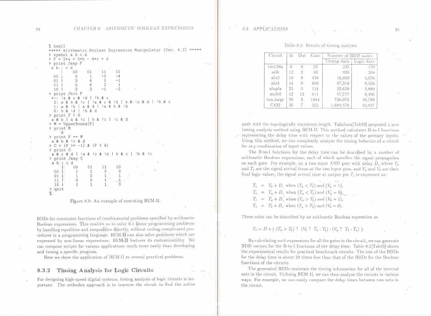
94 CHAPTER 8. :\RITIIMETIC HOOU·.\.\ EXPR£5SJOSS

% bemii ***** Arithmet1e Boolean Expression Manipulator (Ver. 4.2) ***** > symbol a b e d > F = 2•a + 3*b - 4•e + d > print /map F ab e d

00 00 0 01 3 11 5 10 2

01 1 4 6 3

11 -3

0 2

- 1 > print /bit F +-: ! a &: e &: ! d I ! b &: e

10 -4 -1

1 -2

2: a &: b &: !e I !a&: e &: !d I b &: !e &: d I !b &: e 1: a&: !b I a&: d I !a&: b & !d o: b &: !d I !b &: d

> print F > 0 a&: b I a&: !e I b &: !e

> M = UpperBound(F) > pnnt M

6 > print F == M

a &: b &: le &: d

!e &: d

> C = (F >= -1) &: (F < 4) > print C

a &: e &: d I !a &: !e &: Id I b &: e I lb &: le > print /map C ab e d

00 01 11 10

> quit Y.

00 1 1 0 1

01 1 0 0 1

11 0 1 1 1

10 0 1 1 0

Figure 8.9: An example of executing BEM- II.

BDDs for constraint functions of combinatorial problems specified by arithmetic Boolean expressions. This enables us to solve 0-1 linear programming problems by handling equalities and inequalities directly, without coding complicated pro­cedur<'s in a programming language. BE:\1-11 can also solve problems \vhich are expressed by non-linear expressions. BEM-11 features its customizability. We can compose scripts for various applications much more easily than developing

and tuning a specific program. Here we show the application of BE~1 -ll to several practical problems.

8.3 .2 Timing Analys is for Logic Circuits

For d<'signing high-speed digital systems, timing analysis of logic circuits is im­portant. The o rthodox approach is to traverse the circuit to find the active

8 3. APPLICATIOSS 95

Table 8.:2: Hesulb of timing anal~ sis.

Circuit In Out Gate :\umber of BDD nodes Timing data Logic data

cm138a 6 8 29 :l:l) 1:29 sel8 12 2 ·1 :3 <)2(j :268 alu2 10 6 4:31 16,883 4,076 alu4 14 8 809 97,318 9,326

alupla 25 5 114 22,659 2,889 mult6 12 12 411 57,777 9,496

tooJarge 39 3 1044 730,076 10,789 C432 36 7 205 I ,689,576 10,827

path with the topologically maximum l<'ngth. Takahara[Tak93] proposf'd a 11('\\'

timing analysis method using BE~l I I. This met hod calculates B-to-1 functions representing the delay time with respect to the valu<'s of the primary inputs. Using this method. we can completely analyzc the timing behavior of a circuit for any combination of input values.

The B-to-I functions for the delay time can be described by a number of arithmetic Boolean expressions, each of which specifies the signal propagation on each gate. For example, on a two input AND gal<' with delay D, where 7~ and n are the signal arrival times at the two input pins, and Va and \1/, ar<' their final logic values, the signal arrival tirn<' at output pin Tc is expressed as:

Tb + D, when (Ta < Tb) and {Ya- 1),

Ta + D, when (Ta < n) and (Va = 0),

Ta + D, when (Ta > Tb) and (Vb = 1),

Tb + D, when (Ta > n) and (\1/, 0).

These rules can be described by an arithmetic Boolean <'Xpression as

Tc = D + ( (Ta > n) ? (Vb? T,. : n): (Va ? n: Ta) ).

By calculating such expressions for all th<' gates in the circuit, we can gen<'rale BDD vectors for the B-to-I functions of the dday tim<'. Table 8.2[Tak93) shows the experimental results for practical benchmark circuits. The size of the BDDs for the delay time is about 20 times less than that of th<' BDDs for the Boolean functions of the circuits.

The generated BDDs maintain the timing information for all of th<' intC'rnal nets in the circuit. Utilizing BEM-11, we• can then analyze the circuits in various ways. For example, we can easily compare the delay times bC'tween two nets in the circuit.

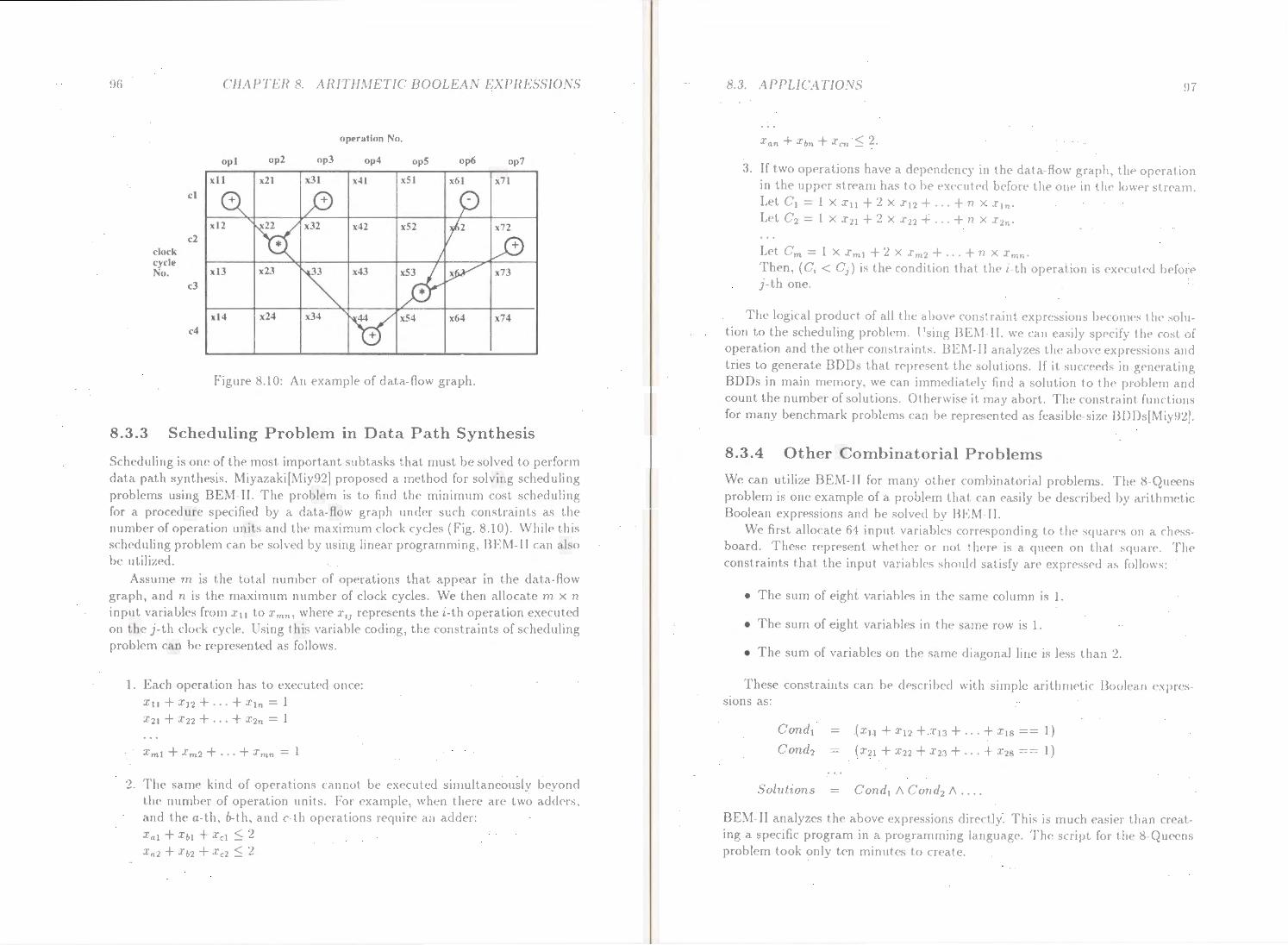
96

clock cycle No.

cl

c2

c3

c4

CHAPTER 8. ARI1'11METIC IJOOLEAS EXPRESSJOSS

operation No.

opt op2 op3 op4 opS op6 op7

xll x21 x31 x41 xS l x61 x71

Figure 8.10: An example of data-flow graph.

8.3.3 Sch eduling Problem in Data Path Synthesis

Sclwduling is one of the most important subtasks that must be solved to perform

data path synthesis. Miyazakif~1 iy92] proposed a method for solving scheduling problems using B EM- II . The problem is to find the minimum cost scheduling for a procedure specified by a data-flo\'>' graph under such constraints as the number of operation units and the maximum clock cycles (Fig. 8.10). W hile this sch<'duling probl<'m can be solved by using linear programming, BEM- IJ can also he ut.ilizcd.

Ass ume m is the total number of operations t hat appear in the data-Row graph, and n is the maximum number of clock cycles. We then allocate m x n

in put va riabl<'s from .r 11 to Xmn, where .r.1 repres<'nts the i-th operation executed on th<' J th clock cycle. Using this variable coding, the cons t raints of scheduling problem ea n be n•presented as follows.

1. Each operation has to executed once:

:ttt + Xt·z + ... + Xtn = 1 X21 + .r22 + ... + X2n = 1

Xml + Xm2 + · · · + Xmn = 1

2. l'he same kind of operations cannot he ex<·cukd simultaneously beyond tlH• number of operation units. For example, when there are two adders, and the a-th, b-t h , and e-t h opcrat ion<> requin· an adder:

Xa l + .l'b l + ;l'cl =:; 2 :l'al + .l'b2 + .l'c2 =:; 2

8.3. APPLICAT/0.\'S

3. If two operations ha\·e a dependency in the data-flow graph, the operation in the upper stream has to bt> t•xecutt•d bt'fon• th(• one in the lower !'I ream.

Let Ct = 1 X I11 + 2 X .r12 + ... + n X .rln·

Let c2 = 1 X I2t + 2 X .r.22 + ... + ll X .r~ ...

Let Cm = 1 X XmJ + 2 X Xm:l + ... + 11 X Xmr~· Then, (C.< C1 ) is the condition that tlw i-th operat1on is executc·d befon• j-th one.

The logical product of all the abovt• constntint t•xpn:ssiolls becorn<'s the solu­tion to the scheduling problem. Usi11g BE.\1-11. we ca11 easily specify the cost of operation and the other constraints. BE~t-11 analyz<'S t h<· abo\·e express1011s a11d tries to generate BDDs that represent t ht• sol ut ions. If it sucn•eds in general ing ODDs in main memory. we can imrnediatt·ly rind a solution to the problem a11d count the number of solutions. Ot hcrwise it may abort. The constraint functions for many benchmark problems can be rcpr<:sented as feasible-size BDDs(~liy92] .

8.3.4 Other Combina toria l Problem s

We can utilize BEM-11 for many other combinatorial problems. Tlw 8-Queens problem is one example of a problem that can easily b<' dc>scribed by arithmetic Boolean expressions and be soht<•d by BEM I I.

We first allocate 64 input variabks corr<'sponding to the squares on a ch<•ss hoard. These represent whf'ther or not there is a quC'<'n on that squar<'. Th<' constraints that the input variables should satisfy arc expressed as follows:

• The sum of eight variables in t.hc sanw column is l.

• The sum of eight variables in the same row is l.

• The sum of variables on the same diagonal line is less than 2.

These constraints can be dcscrib<·d with simple arithmetic Boolcan cxpr<'s­stons as:

Solutions

(XtJ + X12 + Xt3 + ·. · + J't8 == 1)

(x21 + X22 + X23 + ... + X28 == 1)

Cond1 1\ Co11d2 1\ ....

B EM- II analyzes the above expression c.; directly. This is much easier than creat­ing a specific program in a programming languag<!. The: script for the 8-Quccns problem took only ten minutes to cr<'atc.

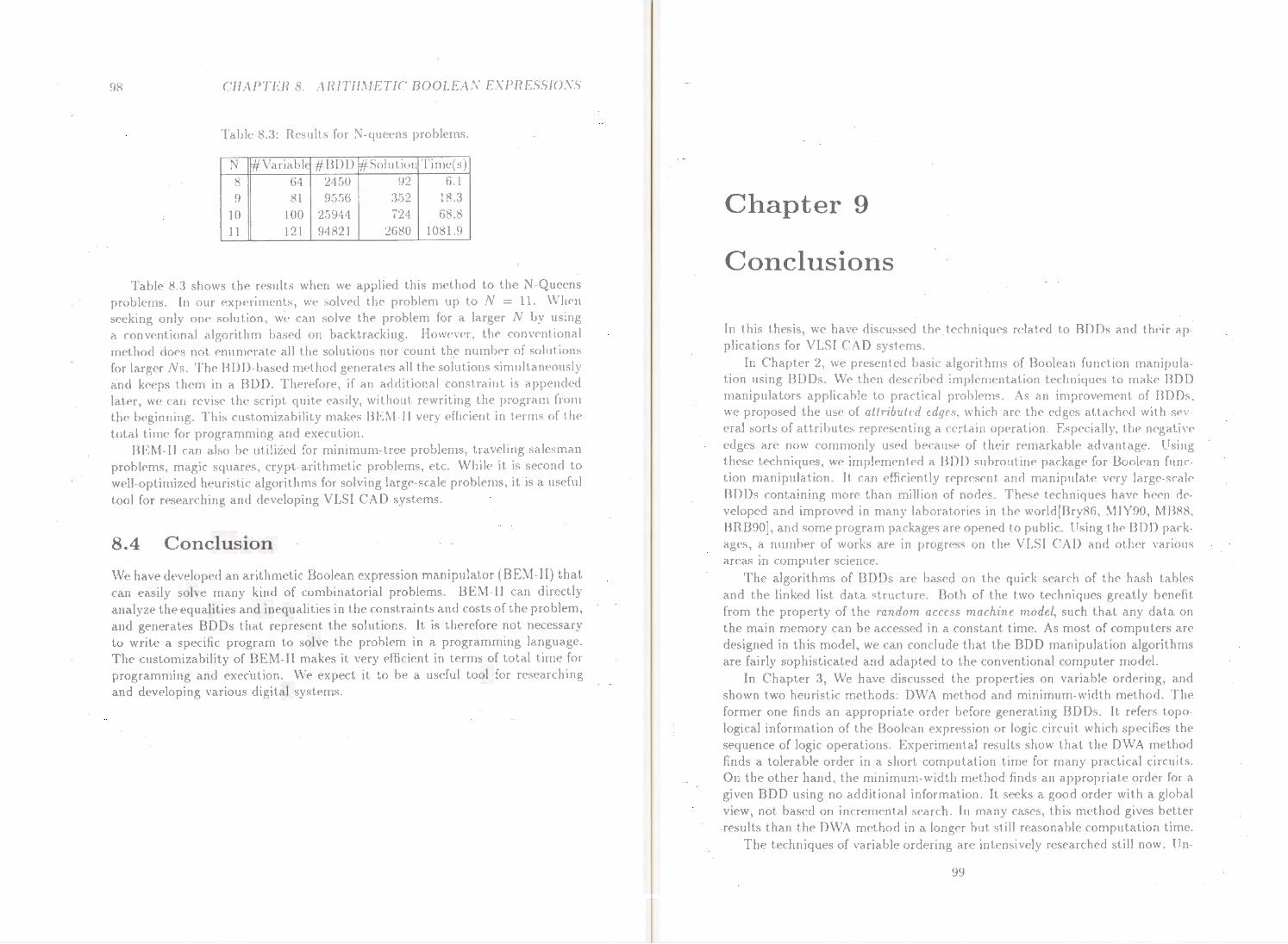
98 CHAPTER 8. ARITTL\!ETf(' BOOLEA.S EXPRESSIOSS

Table 8.3: Results for ~-queens problems.

N f#VariablE #BOO f#Solution Time(s)

8 64 2450 92 6.1

9 81 9556 352 18.3

10 100 25944 724 68.8

11 121 94821 2680 1081.9

Table 8.3 shows the results when we applied this method to the N-Queens problems. In our experiments, we solved the problem up to N = ll. When seeking only one solution, we can solve the problem for a larger N by using a conventional algorithm based on backtracking. However, the conventional method does not enumerate all the solutions nor count the number of solutions for larger Ns. The BDD-based method generat<'s all the solutions simultaneously and keeps them in a BDD. Therefore, if an additional constraint is appended later, we can revise the script quite easily, without rewriting the program from the beginning. This customizability makes BEI\1-II very efficient in terms of the total time for programming and execution.

BEM-II can also be utilized for minimum-tree problems, traveling salesman problems, magic squares, crypt-arithmetic problems, etc. While it is second to wcll-opt imized heuristic algorithms for solving large-scale problems, it is a useful tool for researching and developing YLSI CA 0 systems.

8.4 Conclusion

We have developed an arithmetic Boolean expression manipulator (BEM-II) that can easily solve many kind of combinatorial problems. BEM-11 can directly analyze the equalities and inequalities in the constraints and costs of the problem, and generates BDDs that represent the solutions. It is therefore not necessary to write a specific program to solve the problem in a programming language. The customizability of BEM-II makes it very efficient in terms of total time for programming and execution. We expect it to be a useful tool for researching and developing various digital systems.

Chapter 9

Conclusions

In this thesis, we have discussed the techniques related to BDOs and thei r ap plications for VLSI CA 0 systems.

In Chapter 2, we presented basic algorithms of Roolean function manipula­tion using BOOs. We then described implementation techniques to make BDD manipulators applicable to practical problems. As an improvement of BDDs, we proposed the use of attributed edges, which are the edges attached with sev­eral sorts of attributes representing a certain operation. Especially, the n<'gat iv<' edges are now commonly used because of their remarkable advantage. Using these techniques, we implemented a BOD subroutine package for Boolcan func­tion manipulation. It can efficiently represent and manipulate very large-scale BDDs containing more than million of nodes. These techniques have been de­veloped and improved in many laboratories in the world[Bry86, MJY90, MBR8, BRB90], and some program packages are opened to public. t Tsing the I3DD pack­ages, a number of works are in progress on the YLSI CAD and other various areas in computer science.

The algorithms of BDDs are based on the quick search of the hash tables and the linked list data structure. Both of the two techniques greatly benefit from the property of the random access machine model, such that any data on the main memory can be accessed in a constant time. As most of computers arc designed in this model, we can conclude that the BDD manipulation algorithms are fairly sophisticated and adapted to the conventional computer model.

In Chapter 3, We have discussed the properties on variable ordering, and shown two heuristic methods: DWA method and minimum-width method. The former one finds an appropriate order before generating BDDs. It r<"fers topo­logical information of the Boolean expression or logic circuit which specifies the sequence of logic operations. Experimental results show that the DWA method finds a tolerable order in a short computation time for many practical circuits. On the other hand, the minimum-width method finds an appropriate ord<"r for a given BDO using no additional information. It seeks a good order with a global view, not based on incremental search. In many cases, this method gives better results than the DWA method in a longer but still reasonable computation time.

The techniques of variable ordering arc intensively researched sti ll now. Un-

99

100 CI-I:'\ PT ER 9. COS CL USIOSS

fortunately, it is almost impossible to ha,·e an ultimate method of variable or­dering to always find bc>st order in a practical time. \Ne will make do with some heuristic methods according to the applications.

In Chapter 4, We discussed the representat ion of multi-valued fun ctions. In many applications, we sometimes use ternary-valued functions containing don't cares. We have shown two method of handling don't care; ternary-valued BDDs and BDD pairs, and compared the two by introducing the D-variable. The technique of handling don't care are basic and important for Boolean func tion manipulation in many problems.

BasC'd on the conside ration of don't care, we extended the argument into B­to-1 fun ctions, and presented two mc>thods; MTBDDs and BDD vectors. They can be compared by introducing bit-select ion variables, as well as on the ternary­valued functions. Multi-valued logic manipulation is important to broaden the scop<' of BDD application. Presently, a number of researches are in progress. These techniques are useful not only for VLSI CAD but also for various areas in computer science.

In Chapter 5, we discussed the topic how efficiently transform BDD represen­tation into other data structures. We presented ISOP algorithm for generating prime-irredundant cube sets directly from given BDDs, in contrast to the con­ventional cube set reduction algorithms, which temporarily manipulate redun­dant cube sets or truth tables. The experimental results demonstrate that our method is efficient in terms of time and space. In practical time, we can generate cube sets consisting of more than 1,000,000 literals from multi-level logic circuits which have never previously been flattened into two-level logics. Our method is more than 10 times faster than conventional methods in large-scale examples. It gives quasi-minimum numbers of cubes and literals. In terms of size of the result, the ISOP algorithm may give somewhat larger results than ESPRESSO, but there are many applications in which such an increase is tolerable. Our method can be utilized to transform BDDs into compact cube sets or to flatten multi- level circuits into two-level circuits .

In Chapter 6, we have proposed Ze1·o-Supp1·essed BDDs (0-Sup-BDDs), which arc BDDs based on a new reduction rule. As our understanding of BDDs has deepened, the range of applications has broadened. Besides Boolean functions, we arc often faced with manipulating sets of combinations to deal with many problems, not only in the digital system design but also various areas in com­puter science. 0-sup-BDDs can manipulate sets of combinations more efficiently than using conventional BDDs. This data structure is adapted for the sets of combinations. The effect of 0-Sup-BDDs is remarkable especially when manip­ulating sparse combinations. We discussed the properties of 0-sup-BDDs and their efficiency based on a statistical experiment. We thPn presented the basic operators for 0-sup-BDDs. Those operators are defined as the operations on sets of combinations, which slightly diffc>r from the Boolean function manipulation based on conventional BDDs.

Based on the 0-sup-BDD techniques, we discussed the calculation of unate cube set algebra. We developed efficif'nt algorithms for computing unate cube

10 I

set operations including multiplication and division. and show som<' practical applications. For solving some types of combinatorial prohlt>ms. unate cube se-t algebra is more useful than using COtl\'e'tltional logic operations. \\'c> cxp<'d the unate cube sf't calculator to he utilizt'd as a helpful tool in resenrching and developing \'LSI CAD systems and other various applications.

In Chapter i, an application for VLSI lo~ic synth<'sis was prcsf'ntcd \\'p proposed a fast factorization nwt hod for culw set represent at ion based on U sup­BDDs. Our new algorithm can he <'Xt'CIIt<·d in a time almost proport.ionnl to th<' size of 0 sup-BDDs, which are usunlly much smaller than the numbc·r of literals in the cube set. By using this method, we can q11ickly g~nC'rate multi-level logics from implicit cube sets even for parity functions and full-addC'rs, which have• never bc>cn possible '" 1th tlw conn·nt ional nwt hods. \V<' impi!'IIH'ntc·cl a lit'\\'

rnulti-levf'l logic synthesizer, and cxp0.rimcnt al rf'sults indicak our nwt hod is much fastC'r than convc>ntional met hods and dilfPrt'ncc>s are more> significant for larger-scale problems. Our m<"t hod grc>at ly accC'Ierates mu It i-lc>vC'I logic sv n t hcsis systems and enlarges the scale of applicable> circuits. Then• an' still 'iUill<' room to improve the results. Thus, we have adopted an easy strate-gy for choosing divisors, but more sophisticated strategies may bC' possible. i\1oreover, Boolc>an division method for implicit cube sds is worth invf'stigat ing for this purpose.

In Chapter 8, we presented a helpful tool for the rcsf>arch on computer scie·nc<'. We have developed an arithmetic Boolcan PxprC'ssion manipulator ( BEM -II) t hnt can easily solve many kind of combinatorial problems. Our product features that it calcu lates not only binary logic operation but also arithmetic operations on multi -valued logics, such as addition, subtraction, multiplication, division, equal­ity and inequality. Such arithmetic operations provide simple de•scriptions for various problems. 13EM-II feed s and computes the problems reprc•sented by a set. of equalities and inequalities, which are dealt with using 0-1 linear programming. It is therefore not necessary to write a specific program to so lve the problem in a programming language. We discussed the dala st ructure and algorithms for the arithmetic operations. Finally we presented the sp<'cificat ion of Bf:M-I I and some application examples, such as ttw 8-Quccns problem. Experinwntr~l r<'sults indicate that the customizability of BEl\1-Il makes it very c>fficif'nl in tc>rrns of total time for programming and ex<'cution. We expect it to be a usdul ~ool for researching and developing various digital systems.

102 CHAPTER 9. C'OXCLL 7SIOSS

Bibliography

[Ake78] S. B. Akers. Binary decision diagram. IEEE Trans. on Compul e1·s, Vol. C-27, No. 6, pp. 509- 516, June 1978.

[BC94] R. E. Bryant and Y.-A. Chen. Verification of arithmetic function!'i with binary moment diagrams. Technical report, CarncgiC' Mc,llon University, May 1994.

[BCMD90] J. R. Burch, E. M. Clarke, K. L. McMillan, and D. L. Dill. Sequen­tial circuit verification using symbolic model checking. In Proc. of 27th AGM/IEEE Design Automation Conference {DAC'90}, pp. 46- 51, June 1990.

[BF85] F. Brglez and H. Fujiwara. A neutral netlist of 10 combinational circuits. In Proc. of 1985 IEEE International Symposium Ci1·c1tit and Systems (ISCAS'85), Special Session on A TPG and Fault Sim­ulation, June 1985.

[BFG+93] R. I. Bahar, E. A. Frohm, C. M. Gaona, G. D. Hachtcl, E. Macii, A. Pardo, and F. Somenzi. Algebraic decision diagrams and their applications. In Proc. of IEEE/ A CM International Confenncc on Computer-Aided Design (ICCAD-93), pp. 188 191, Novcmlwr 1993.

[BHMSV84] R. K. Brayton, G. D. Hachtel, C. T. McMullen, and A. L. Sangiovanni-Vincentelli. Logic Minimization Alg01·ithms for VLS/ Synthesis. Kluwer Academic Publishers USA, 1984.

[BRB90] K. S. Brace, R. L. Rudell, and R. E. Bryant. Efficient implemen­tation of a BDD package. In Proc. of 27th A CM/IEEE Design Automation Conference {DAC'90}, pp. 40- 45, June 1990.

[BRKM91] K. M. Butler, D. E. Ross, R. Kapur, and M. R. Mercer. Heuristics to compute variable orderings for efficient manipulation of ordered binary decision diagrams. In Proc. of 28th AGM/IEEE Design Automation Conference (DAC'91}, pp. 417 420, June 1991.

[Bry86] R. E. Bryant. Graph-based algorithms for Boolean function ma­nipulation. IEEE Trans. on Computers, Vol. C-35, No. 8, pp. 677-691, August 1986.

103

101 BTBUOGRA PHY

[13ry91] R. E. 13ryant. On the complexity of \'LST implementations and graph r<'pr<'S<'ntations of 13oolean functions with application to in­teger multiplication. IEEE Trans. on Computers, Vol. C-40, No. 2, pp. 20.5 213, February 1991.

[BSVW87) R. K. Drayton, R. R. A. Sangiovanni-Vincentelli, and A. R. Wang. MIS: A multiple-level logic optimization system. IEEE Tmns. on Computer-Aided Design, Vol. CAD-6, No. 6, pp. 1062- 1081, November 1987.

[CB89) K. Cho and R. E. Bryant. Test pattern generation for sequen­tial MOS circuits by symbolic fault simulation. In Proc. of 26th AGM/IEEE Design Automation Confe1·ence (DAC'89}, pp. 418-423, June 1989.

[CJIJ+9o) H. Cho, G. D. Hachtel, S.-W. Jeong, B. Plessier, E. Schwarz, and F. Somenzi. ATPG aspects of FSM verification. In Proc. of IEEE/ A CM International Conference on Computer-Aided Design (ICCAD-90), pp. 134- 137, November 1990.

[CM92] 0. Coudert and J. C. Madre. A new graph based prime computa­tion technique. In T. Sasao, editor, New Trends in Logic Synthesis, chapter 2, pp. 33-57. Kluwer Academic Publishers USA, 1992.

[CMF93) 0. Coudert, J. C. Madre, and H. Fraisse. A new viewpoint of two-level logic optimization. In Pmc. of 30th AGM/IEEE Design Automation Conference (DAC'93), pp. 625-630, June 1993.

[CMZ+93] E. M. Clarke, K. L. McMillan, X. Zhao, M. Fujita, and J. Yang. Spectral transforms for large Boolean functions with applications to technology mapping. In Proc. of 30th A CM/IEEE Design A u­tomation Conference (DA C'93}, pp. 54- 60, June 1993.

[dG86] A. J. de Geus. Logic synthesis and optimization benchmarks for the 1986 DAC. In Proc. of 231·d A CM/IEEE Design A utomalion Conference (DAC'86}, pp. 78, June 1986.

[FFK88) M. Fujita, H. Fujisawa., and N. Kawato. Evaluation and improve­ment of Boolean comparison method based on binary decision diagrams. In P1·oc. of IEEE/ A CM International Conference on Comp1Lie1·-A ided Des1'gn (ICCAD-88}, pp. 2- 5, November 1988.

(F.l\fl\91) ~1. Fujita, Y. Matsunaga, and T. I<akuda. On variable ordering of binary decision diagrams for the application of multi-level logic synthesis. Tn Proc. of IEEE The European Conference on Design Jhllomation (EDAC'91}, pp. 50 54, February 1991.

BIBLIOGRAPHY 105

[FS87] S. J. Friedman and K. J. Supowit. Finding the optimal variable or­dering for binary decision diagrams. In Proc. of 24lh A CM/lEE£ Design Automation Conference (DAC'87}, pp. 348 356, June 1987.

[HC074) S. J. Hong, R. G. Cain, and D. L. Ostapko. MINT: A heuristic approach for logic minimization. IBM Journal of Research and Development, Vol. 18, No. 5, pp. 443- 458, 1974.

[HMPS94) G. D. Hachtel, E. Macii, A. Pardo, and F. Somenzi. Proba­bilistic analysis of large finite state machines. In Proc. of 31st A CM/IEEE Design Automation Confe1·ence (DA C'94), pp. 270 275, June 1994.

[Ish92) N. Ishiura. Synthesis of multi-level logic circuits from binary deci­sion diagrams. In Proc. of Synthesis and Simulation Meeting and International Interchange (SASIMI'92, Japan), pp. 74 83, March 1992.

[ISY91) N. Ishiura, H. Sawada, and S. Yajima. Minimization of binary decision diagrams based on exchanges of variables. In Proc. of IEEE/ A CM International Conference on Computer-Aided Design (ICCAD-91) , pp. 472- 475, November 1991.

[IY90) N. Ishiura and S. Yajima. A class of logic functions express­ible by a polynomial-size binary decision diagrams. In Proc. of Synthesis and Simulation Meeting and International lnt e1·change (SASIM/'90, Japan) , pp. 48-54, October 1990.

[IYY87) N. Ishiura, H. Yasuura, and S. Yajima. High-speed logic simulation on vector processors. IEEE Tmns. on Computer-Aided Design, Vol. CAD-6, No. 3, pp. 305-321, May 1987.

(JT92] R. P. Jacobi and A. M. Trullemans. Generating prime and irrcdun­dant covers for binary decision diagrams. In Proc. of IEEE The European Conference on Design Automation (EDA C'92}, pp. I 04 108, March 1992.

[LCM89) P. 1ammens, 1. J. Claesen, and H. D. Man. Tautology checking benchmarks: Results with TC. In Proc. of iF/ P International Workshop on Applied Formal Methods for Cornet VLSI Design, pp. 600 604, November 1989.

[1192) H.-T . 1iaw and C.-S. Lin. On the OBDD-representation of general Boolcan functions. IEEE Tmns. on Computers, Vol. C-4 l, No. 6, pp. 661 - 664, June 1992.

106

[LPV93]

[LS90]

[MB88]

[MF89]

[Min90]

[Min93a]

[Min93b]

[MIY89J

[MIY90]

[Miy92]

BIBLIOGRAPHY

Y.-T. Lai, M. Pedram, and S. B. Vrudhula. FGILP: An inte­ger linear program solver based on function graphs. In P1·oc. of IEEE/ A CM International Conference on Compule1·-A ided Design (/CCAD-93}, pp. 685 689, November 1993.

B. Lin and F. Somenzi. Minimization of symbolic relations. In P1·oc. of IEEE/AGM fntemational Confe1·ence on Computer-Aided Design (!CCA D-90}, pp. 88- 91, November 1990.

J. C. Madre and J. P. Billon. Proving circuit correctness us­ing formal comparison between expected and extracted behaviour. In Proc. of 25th A CM/IEEE Design A 1tlomation Conference {DAC'88}, pp. 205 210, June 1988.

Y. Mat.sunaga and M. Fujita. i\1ulti-levcllogic optimization using binary decision diagrams. In Proc. of IEEE/ A CM International Confe1·ence on Computer-Aided Design (!CCAD-89}, pp. 5.56-5.'59, November 1989.

S. Minato. Shared binary decision diagrams for efficient Boolcan function manipulation. Master's thesis, Department of Informa­tion Science, Faculty of Engineering, Kyoto University, February 1990.

S. Minato. BEM-II:an arithmetic Boolean expression manipulator using BOOs. IEJCE Tmns. Fundamentals, Vol. E76-A, No. 10, pp. 1721 1729, October 1993.

S. Minato. Zero-suppressed I3DDs for set manipulation in combi­natorial problems. In Proc. of 30th A CM/IEEE Design A utoma­lion Conference {DA C'93}, pp. 272-277, June 1993.

S. Minato, N. lshiura, and S. Yajima. Symbolic simulation using shared binary decision diagram. In Record of the 1989 IEJCE Fall Conference (in Japanese), pp. 1.206-207, SA 7-5, September 1989.

S. Minato, N. Ishim·a, and S. Yajima. Shared binary decision diagram with attributed edges for efficient Boolean function ma­nipulation. In P1·oc. of 27th A Clvfj!EEE Design A ulomation Con­ference (DAC'90}, pp. 52- 57, June 1990.

T. Miyazaki. Boolean-bascd formulation for data path synthesis. In P1'0c. of IEEE Asia-Pacific Conference on Ci1·cuits and Systems (APCCAS'92}, pp. 201 205, December 1992.

BIBLIOGRA.PH)' 107

[t\1KLC87] S. t\luroga, Y. Kambayashi. II. C. Lai, and J. N. C'ullirwy. The transduction method design of logic net works hased 011 permis­sible functions. IEEE Trans. on Computers, Vol. C-38, No. 10, pp. 1404 1424, June 1987.

[Mor70] E. Morreale. Recursive operators for prime implicant and irre­dundant normal form determination. IEEE Tmns. on Computers, Vol. C-19, No. 6, pp. 504 509, June 1970.

[MSB93] P. McGeer, J. Sanghavi, and R. K. Brayton. Espresso-signature: A new exact minimizer for logic functions. In Proc. of 30th AGM/IEEE Design Automation Conference (DAC'9.1}, pp. 618 624, June 1993.

[MWBSV88] S. Malik, A. R. Wang, R. f\. Brayton, and A. L. Sangiovanni­Vincentelli. Logic verification using binary decision diagrams in a logic synthesis cnvironnwnt. In Proc. of IEEl'J'/A C'Af Interna­tional Conference on Computer-Aided Design (ICCAD-88}, pp. 6 9, November 1988.

[Oku94]

[Rud93]

[Tak93]

[THY93]

[TIY91]

H. G. Okuno. Reducing combinatorial explosions in solving search­type combinatorial problems with binary decision diagram. Tmns. of Information Processing Society of Japan (JPSJ), (in Japanese), Vol. 35, No. 5, pp. 739- 753, May 1994.

R. Rudell. Dynamic variable ordering for ordered binary decision diagrams. In Proc. of IEEE/ A CM International Confe1·encc on Computer-Aided Design {JCCAD-93), pp. 42 47, November 1993.

A. Takahara. A timing analysis method for logic circuits. In Record of the 1993 IE!CE Spring Conference (in Japan ese), pp. 1.120, A- 20, March 1993.

S. Tani, K. Hamaguchi, and S. Yajima. The complexity of the op­timal variable ordering of a shared binary decision diagram. Tech­nical Report 93-6, Department of Information Science, Faculty of Science, University of Tokyo, December 1993.

N. Takahashi, N. Ishiura, and S. Yajima. Fault simulation for multiple faults using BDD representation of fault sets. In P1·oc. of IEEE/ A CM International Conference on Computer-Aided Design (ICCAD-91}, pp. 550-553, November 1991.

108 BTHLIOGRAPHY

Acknowledgment

I would like to express my sincere appreciation to Professor Shuzo Yajima of Kyoto University for his continuous guidance, interesting suggestions, accurate criticisms and encouragements during this research.

I would also like to express my thanks to Dr. Nagisa Ishiura of Osaka Univer­sity who introduced me to the research field of VLSI CAD and BOOs, and has been giving me invalu; ble suggestions, accurate criticisms and encouragements throughout this research.

I also acknowledge interesting comments that I have received from Profes­sor Hiromi IIiraishi of Kyoto Sangyo University, Professor Hiroto Yasuura of Kyushuu University, and Associate Professor Naofumi Takagi of Nagoya Univer­sity.

I would like to thank Dr. Kiyoharu Hamaguch, Mr. Koich Yasuoka and Mr. Shoichi Hirose of Kyoto University, Associate Professor Hiroyuki Ochi of Hiroshima City University, Mr. Yasuhito Koumura of Sanyo Corporation and Kazuya loki of IBM Japan Corporation for their interesting discussions and collaborations in implementing a BOO program package in Chapter 2.

I am indebted to Professor Randal E. Bryant of Carnegie Mellon University who introduced BDD techniques into the VLSJ CAD. I started this research with his papers and received helpful comments from him.

I would also like to thank Dr. Masahiro Fujita and Mr. Yusuke Matsunaga of Fujitsu Corporation, who started to work on BDDs in early time. I referred their papers many times, and sometimes had fruitful discussions with them.

I am grateful to Professor Saburo Muroga of University of Illinois at Urbana­Champaign and Professor Tsutomu Sasao of Kyushu Institute of Technology for their instructive comments and discussions on the techniques of logic synthesis.

I also wish to thank Dr. Olivicr Coudert of DEC Paris Research Laboratory for his discussions on the implicit set representation, which led to the idea of Zero-suppressed BDDs in Chapter 6.

I would like to thank Professor Gary D. Hachtel and Associate Professor Fabio Somenzi of University of Colorado at Boulder for their fruitful discussions on the application of BOOs for combinatorial problems in Chapter 8.

I am also grateful Professor Robert K. Brayton, Or. Patrik McGeer, Dr. Yoshinori Watanabe and Mr. Yuji Kukimoto of University of C'alfornia at Ikrkc­ley for their interesting discussions and suggestions on the techniques of logic synthesis based on BDDs in Chapter 5 and 7.

109

110 A C'I\.\'0\ \'LEDG.\1£.\'T

Thanks are also due to my colleagues in ~TT Research Laboratories. I grate­fully acknowledge the collaboration with Dr. Toshiaki Miyazaki and Dr. Atsushi Takahara in developing and evaluating the BEM-II program in Chapter 8. I am also grateful to Mr. Hiroshi G. Okuno and Mr. Masayuki Yanagiya for their interests in the BEM-II applications. I also thank Mr. Noriyuki Takahashi for his helpful comments on the application of 0-sup-BDDs for fault simulation in Chapter 6.

I express special gratitude to Mr. Yasuyoshi Sakai, Dr. Osamu Karatsu, Mr. Tamio lloshino, Mr. Makoto Endo, and all the other members of NTT Advanced LSI Laboratory for giving me an opportunity to write this thesis, and for their helpful advices and encouragements.

Thanks are due to all the members of the Professor Yajima's Laboratory, especially to Mr. Yasuhiko Takcnaga, Mr. Hiroyuki Ogino and Mr. Kazuyoshi Takagi, for their discussions and helpful supports throughout this research.

Lastly, I thank my parents and my wife for their patience, support and encouragement.

List of Publications by the Author

Major Publications

1. S. Minato, N. lshiura, and S. Yajima. Fast tautology checking using shared BDD. In Proc. of IFIP International Wot·kshop on Applied For·mal Meth­ods for Correct VLSI Design, pp. 107- 111, November 1989.

2. S. Minato, N. IshiUI·a, and S. Yajima. Shared binary decision diagram with attributed edges for efficient Boolean function manipulation. In P1·oc. of 27th AGM/IEEE Design Automation Conference {DA C'90}, pp. 52 57, June 1990.

3. S. Minato, N. Ishiura, and S. Yajima. Shared binary decision diagrams for efficient Boolean function manipulation. Trans. of Information Processing Society of Japan (IPSJ) , {in Japanese), Vol. 32, No. 1, pp. 77-85, January 1991.

4. S. Minato. Minimum-width method of variable ordering for binary decision diagrams. IEICE Trans. Fundamentals, Vol. E75-A, No. 3, pp. 392 399, March 1992.

5. S. Minato. Fast generation of irredundant sum-of-products forms from bi­nary decision diagrams. In ?roe. of Synthesis and Simulation Meeting and International Interchange (SASIM/'92, Japan), pp. 64- 73, April 1992.

6. S. Minato. Fast generation of prime-irredundant covers from binary deci­sion diagrams. IEICE Trans. Fundamentals, Vol. E76-A, No. 6, pp. 967 973, June 1993.

7. S. Minato. BEM-II: An arithmetic Boolean expression manipulator using BDDs. IEICE Trans. Fundamentals, Vol. E76-A, No. 10, pp. 1721- 1729, October 1993.

8. S. Minato. Fast weak-division method for implicit cube representation. In Proc. of Synthesis and Simulation Meeting and International Interchange {SASIM/'93, Japan), pp. 423- 432, October 1993.

111

112 LIST OF PUBLICATIONS

9. S. Minato. Techniques for BOO manipulation on computers. The Journal of Information Processing Society of Japan (IPSJ}, (in Japanese), Vol. 34, No. 5, pp. 593 599, May 1993.

10. S. Minato. Zero-suppressed BOOs for set manipulation in combinatorial problems. In Proc. of 30th A CM/IEEE Design Automation Conference (DAC''99}, pp. 272 277, June 1993.

11. S. Minato. Calculation of unate cube set algebra using zero-suppressed BOOs. In Proc. of 31st AGM/IEEE Design Automation Conference (IJA C'94}, pp. 420- 424, J une 1994.

Technical Reports

1. S. Minato, N. Ishiura, and S. Yajima. Shared binary decision diagram for efficient Boolean function manipulation. Technical Report of IEICE on Vl"S I Design Technologies, {in Japanese), Vol. 89, No. 338, pp. 39-46, VLD89 80, December 1989.

2. S. Minato. Fast generation of irredundant sum-of-products from binary decision diagrams. Technical Report of IEICE on VLSI Design Technolo­gies, (in Japanese), Vol. 91, No. 376, pp. 25 32, VLD9l 107, December 1991.

3. S. Minato. Minimum-width method of variable ordering for binary decision diagram reduction. In Proc. of IEICE The 4th f(A RUIZA WA l1Vorkshop on Cirwits and Systems, {in Japanese), pp. 271 276, April 199 J.

4. S. Minato. Techniques of Boolean function manipulation based on binary decision diagrams. In Proc. of IEICE The 5th I\'ARUIZAWA Workshop on Circuits and Systems {in Japanese}, pp. 161 166, April 1992.

5. S. Minato. BEM-11: An arithmetic Boolean expression manipulator using binary decision diagrams. Technical Report of IEICE on Computation, (in Japanese), Vol. 92, No. 447, pp. 25 32, COl\ IP92 75, January 1993.

6. S. Minato. Fast weak-division method for implicit cube sets using zero­supprcss<'d BDDs. Technical Report of IEICE on VLSI Design Technolo­gtcs, (m. Japanese), Vol. 93, No. 501, pp. 55 62, VLD93 200, ~larch 1994.

Conve ntion Records

l. S. Minato, N. Ishiura, and S. Yajima. Symbolic simulator using truth table representation. In Reco1·d of 97th IPSJ National Convention, {in Japanese}, pp. 1757- 1758, 3U 2, SE>plcmbE>r 1988.

CO.'VVENTION RECORDS 113

2. S. Minato, N. lshiura, and S. \ajima On Boolcan function manipulation using shared binary decision d1agram. In R("('orYi of 3blh IPSJ .Vatwnal Convention, (in Japanese), pp. 1371 I:l72, SS 9, ~tarch 1989.

3. S. Minato, N. lshiura, and S. Yajima. Symbolic simulation using shared binary decision diagram. In Rl:cord of the 1989 IEIC'E Fall C'onfer·cnce, (in Japanese), pp. 1.206 1.207, SA 7 5, September 1989.

4. S. Minato, N. Ishiura, and S. Yajima. Variable shiftcr for shared binary decision diagram. In Record of the /990 IEIC'E Spn"ng Confe7'Cnce, (in Japanese), pp. 1.115, A 115, March 1990.

5. S. Minato. Minimum-width nwlhocl of variilblc ordering for shar<'d bi ­nary decision diagrams. In RfcorYI of 42nd I PS.J National Convention, (111 Japanese), pp. 6.158, 2J .), :\1arrh 1991.

6. S. Minato. Fast generation of itrcdundaut stun-of products using binary decision diagrams. In Record of 4 'lrd IJ>SJ Vational Convcnt10n, (in Japanc.w ), pp. 6.179, 2R- 10, October 1991.

7. S. Minato. Variable shifter for sharcd binary dc•cision diagram. In Record of the 1992 IEICE Fall Confcrcncr, (m Japanese), pp. 1.51, A- .51, Scptcm ber 1992.

8. S. Minato. Zero-suppressed BDDs and their applications. In Record of the 1993 IEICE Spring Conference, (in Japanese), pp. 1.368 1.369, SA- 2 2, March 1993.

9. S. Minato. Complemental set OJ)('rations for zero-suppressed bdds. In Record of the 1994 IEICE Sp1·ing Confcrcnrc, (in Japanese), pp. J.Jttl, A 140, March 1.994.