timewarp rigid body simulation - cs.mcgill.cacarl/rigidbody.pdf · timewarp rigid body simulation...

MITSUBISHI ELECTRIC RESEARCH LABORATORIEShttp://www.merl.com

Timewarp Rigid Body Simulation

Brian Mirtich

TR2000-17 December 2000

AbstractThe traditional high-level algorithms for rigid body simulation work well for moderate numbersof bodies but scale poorly to systems of hundreds or more moving, interacting bodies. The prob-lem is unnecessary synchronization implicit in these methods. Jeffersons timewarp algorithm(Jefferson 85) is a technique for alleviating this problem in parallel discrete event simulation.Rigid body dynamics, though a continuous process, exhibits many aspects of a discrete one.With modification, the timewarp algorithm can be used in a uniprocessor rigid body simulator togive substantial performance improvements for simulations with large numbers of bodies. Thispaper describes the limitations of the traditional high-level simulation algorithms, introducesJeffersons algorithm, and extends and optimizes it for the rigid body case. It addresses issuesparticular to rigid body simulation, such as collision detection and contact group management,and describes how to incorporate these into the timewarp framework. Quantitative experimentalresults indicate that the timewarp algorithm offers significant performance improvements overtraditional high-level rigid body simulation algorithms, when applied to systems with hundredsof bodies. It also helps pave the way to parallel implementations, as the paper discusses.

SIGGRAPH 00

This work may not be copied or reproduced in whole or in part for any commercial purpose. Permission to copy in whole or in partwithout payment of fee is granted for nonprofit educational and research purposes provided that all such whole or partial copies includethe following: a notice that such copying is by permission of Mitsubishi Electric Research Laboratories, Inc.; an acknowledgment ofthe authors and individual contributions to the work; and all applicable portions of the copyright notice. Copying, reproduction, orrepublishing for any other purpose shall require a license with payment of fee to Mitsubishi Electric Research Laboratories, Inc. Allrights reserved.

Copyright c!Mitsubishi Electric Research Laboratories, Inc., 2000201 Broadway, Cambridge, Massachusetts 02139

MERLCoverPageSide2

MERL – A MITSUBISHI ELECTRIC RESEARCH LABORATORYhttp://www.merl.com

Timewarp Rigid Body Simulation

Brian Mirtich

TR-2000-17 April 2000

AbstractThe traditional high-level algorithms for rigid body simulation work well for moderate

numbers of bodies but scale poorly to systems of hundreds or more moving, interactingbodies. The problem is unnecessary synchronization implicit in these methods. Jef-ferson’s timewarp algorithm [22] is a technique for alleviating this problem in paralleldiscrete event simulation. Rigid body dynamics, though a continuous process, exhibitsmany aspects of a discrete one. With modification, the timewarp algorithm can be usedin a uniprocessor rigid body simulator to give substantial performance improvementsfor simulations with large numbers of bodies. This paper describes the limitations of thetraditional high-level simulation algorithms, introduces Jefferson’s algorithm, and ex-tends and optimizes it for the rigid body case. It addresses issues particular to rigid bodysimulation, such as collision detection and contact group management, and describeshow to incorporate these into the timewarp framework. Quantitative experimental re-sults indicate that the timewarp algorithm offers significant performance improvementsover traditional high-level rigid body simulation algorithms, when applied to systemswith hundreds of bodies. It also helps pave the way to parallel implementations, as thepaper discusses.

In SIGGRAPH 00 Conference Proceedings, July 2000

This work may not be copied or reproduced in whole or in part for any commercial purpose. Permission to copy inwhole or in part without payment of fee is granted for nonprofit educational and research purposes provided that allsuch whole or partial copies include the following: a notice that such copying is by permission of Mitsubishi ElectricInformation Technology Center America; an acknowledgment of the authors and individual contributions to the work;and all applicable portions of the copyright notice. Copying, reproduction, or republishing for any other purpose shallrequire a license with payment of fee to Mitsubishi Electric Information Technology Center America. All rights reserved.

Copyright c Mitsubishi Electric Information Technology Center America, 2000201 Broadway, Cambridge, Massachusetts 02139

1. First printing, 11 January 20002. Revision, 20 April 20003. Tech Report, TR2000-17, 28 April 2000

1

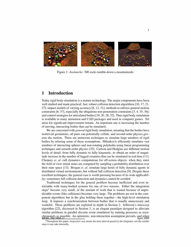
Figure 1: Avalanche: 300 rocks tumble down a mountainside.

1 IntroductionToday rigid body simulation is a mature technology. The major components have beenwell studied and made practical: fast, robust collision detection algorithms [10, 17, 21,27]; impact models of varying accuracy [8, 12, 31]; methods to enforce general motionconstraints [6, 37], especially the ubiquitous non-penetration constraints [3, 4, 35, 36];and control strategies for articulated bodies [19, 20, 28, 32]. Thus rigid body simulationis available in many animation and CAD packages and used in computer games. Yetareas for significant improvement remain. An important one is increasing the numberof moving, interacting bodies that can be simulated.

We are concerned with general rigid body simulation, meaning that the bodies havenontrivial geometries, all pairs can potentially collide, and second-order physics gov-erns the motion. There are numerous techniques to simulate large numbers of rigidbodies by relaxing some of these assumptions. Milenkovic efficiently simulates vastnumbers of interacting spheres and non-rotating polyhedra using linear programmingtechniques and zeroeth-order physics [25]. Carlson and Hodgins use different motionlevels of detail, from fully dynamic to fully kinematic, to obtain an order of magni-tude increase in the number of legged creatures that can be simulated in real time [11].Chenney et. al. cull dynamics computations for off-screen objects; when they enterthe field of view initial states are computed by sampling a probability distribution overtheir state space [13]. Brogan et. al. simulate large herds of fully dynamic agents indistributed virtual environments, but without full collision detection [9]. Despite theseexcellent techniques, the general case is worth pursuing because of its wide applicabil-ity; sometimes full collision detection and dynamics cannot be avoided.

Traditional techniques for the general problem become inefficient and even in-tractable with many-bodied systems for one of two reasons. Either the integrationsteps1 become very small, or the amount of work that is wasted because of unpre-dictable events (like collisions) becomes very large. The problems are not in the com-ponent algorithms but in the glue holding them together—the high-level simulationloop. It imposes a synchronization between bodies that is usually unnecessary andwasteful. These problems are explored in depth in Section 2. Jefferson’s timewarpalgorithm [22], discussed in Section 3, is an elegant paradigm designed to alleviatesimilar problems in parallel discrete event simulation by running processes as asyn-chronously as possible. An optimistic, non-interaction assumption prevails, and when

1Throughout this paper, integration step means the time interval passed to the integrator, not the smallersteps it may take internally.

MERL-TR-2000-17 April 2000

2

it is violated only the computation that is provably invalid is undone. Although rigidbody dynamics is a continuous process, it exhibits many traits of a discrete process.With some modification, the timewarp algorithm can be used in rigid body simulators,improving both their speed and scalability. The method is described in Section 4, andSection 5 presents results from an actual implementation.

Timewarp rigid body simulation also supports the long-range goal of a highly paral-lel implementation. Rigid body simulation offers unlimited potential for modeling thecomplex and unanticipated interactions of rich virtual environments, but current tech-nology cannot support this. Meeting this challenge will certainly require a multipro-cessor approach, with perhaps hundreds of processors computing motion throughoutthe environment. Such a simulation farm is akin to the rendering farms that generatetoday’s high quality computer animation. Section 6 touches on these issues.

2 Simulation DiscontinuitiesThe dominating computation in a rigid body simulator is that of numerically integratingthe dynamic states of bodies forward in time. The differential equations of motion havebeen known for centuries; the true difficulty lies in processing simulation discontinu-ities, here defined as events that change the dynamic states or the equations of motionof some subset of the bodies. Examples include collisions, new contacts, transitionsbetween rolling and sliding, and control law changes. Integrators cannot blithely passthrough discontinuities. Instead the integration must be stopped, the states or equationsof motion updated, and then the integrator restarted from that point. Compounding thiscomplication is the fact that the times of most discontinuities are impossible to predict.Thus the integration must be interrupted even more frequently than the rate at whichdiscontinuities occur, just to check if they have occurred. There are two common ap-proaches for coping with discontinuities, both of which have been shown practical formoderate numbers of bodies.

2.1 Retroactive DetectionRetroactive detection (RD) is the most common approach to handling discontinuities.The simulator takes small steps forward and checks for discontinuities after each step[2, 23]. For example, inter-body penetration indicates that a collision occurred at sometime during the most recent integration step. A root finding method localizes the exactmoment of the discontinuity. After resolution, the integration is restarted from thatpoint. All of the bodies must be backed up to their states at the time of the disconti-nuity because (1) the discontinuity may have affected their motion, and (2) the bodiesdirectly involved in the discontinuity must certainly be backed up to this time, andthere is no framework for maintaining bodies at different times—the bodies must bekept synchronized. The first problem is avoidable by bounding a discontinuity’s influ-ence. A certain collision may provably have no influence on the motion of a distantbody over the current integration step. However, the second problem is fundamental toRD. It does not suffice to maintain states at two different times, the time of the discon-tinuity and the time at the end of the step, because multiple discontinuities can occur at


3

different times in a single step. Also, earlier discontinuities may cause or prevent laterones, and it is hard to determine which one occurred first without localizing the timesof each. In practice, all bodies are backed up to the point of each discontinuity. Thismethod is correct since it eventually processes all real discontinuities and no spuriousones, and Baraff has shown it to be efficient and eminently practical for moderate num-bers of interacting bodies [5]. As the number of bodies increases, so does the the rateof discontinuities, and the wasted work per discontinuity increases since more bodiesmust be backed up. Shrinking the step size to reduce the amount of backup is not agood solution as we shall see. Eventually RD becomes intractable due to the amountof wasted work.

2.2 Conservative AdvancementConservative advancement (CA) is an alternative to RD based on the idea of neverintegrating over a discontinuity. Conservative lower bounds on the times of disconti-nuities are maintained in a priority queue sorted by time, and the simulator repeatedlyadvances all simulated bodies to the bound at the front of the queue. The simulatortends to creep up to each discontinuity, taking smaller steps as it gets closer. VonHerzen et. al. use this approach to detect collisions between time-dependent paramet-ric surfaces [18], and Mirtich uses it to support impulse-based simulation [26]. Snyderet. al. use a related approach to locate multi-point collisions by using interval inclu-sions to bound surfaces in time and space [33]. Finally, CA forms the basis for kineticdata structures pioneered by Basche et. al. [7]. These are used to solve a host of prob-lems from dynamic computational geometry, such as maintaining the convex hull ofa moving point set, by maintaining bounds on when the combinatorial structure maychange. For rigid body simulation the advantage of CA is that it does not waste workby integrating bodies beyond a discontinuity. Unfortunately, as the number of bodiesincreases the average time to the next discontinuity check decreases, and the problemis exacerbated since it is difficult to compute tight bounds on times of collisions andcontact changes. Stopping the integration of all bodies at each check is very inefficient,and CA becomes intractable with many bodies.

2.3 Step Sizes and EfficiencyFigure 2 graphically demonstrates the problem with small integration steps. It showsthe computational cost of computing the 10-second trajectory of a ballistic, tumblingbrick using a fifth order adaptive Runge-Kutta integrator [30] under various step sizes.The two qualitatively similar curves correspond to different integrator error tolerances.At small step sizes the integrator does not need to subdivide the integration step intosmaller pieces to meet the error tolerance. Thus computation is proportional to thenumber of invocations: halving the step size doubles the work. At large step sizes theintegrator breaks the requested step into smaller pieces to meet the error tolerance, socomputation is insensitive to step size. Unfortunately, even with a moderate number ofbodies, a simulator’s operating point is to the left of the elbow in these curves. Thus,reducing the step size significantly increases computational cost.


4

1E+05

1E+06

1E+07

1E+08

1E-04 1E-03 1E-02 1E-01 1E+00 1E+01

com

puta

tiona

l cos

t (flo

ps)

integration timestep (seconds)

Brick Integration Experiment

(30 Hz)

eps=1.0E-4

eps=1.0E+0

Figure 2: Cost of computing the trajectory of a brick versus integration step size (epsis the integrator error tolerance).

3 The Timewarp AlgorithmThe problems of RD and CA result from unnecessary synchronization. Each discon-tinuity affects only a small fraction of the bodies, yet under RD every body must bebacked up when a discontinuity occurs, and under CA integration of every body muststop for a discontinuity check. The inefficiencies are tolerable as long as there are nottoo many bodies. Similar issues arise in discrete event simulation (DES) , which is of-ten applied to very large models such as cars on a freeway system. These simulationsare often done in parallel or distributed settings. The simulated agents are partitionedamong a number of processors, each of which advances its agents forward in time.There are causality relationships that must be preserved (e.g. a car suddenly brakingcauses the car behind it to brake), and the crux of the problem is that one agent maytrigger an action of another agent on a different processor. Obviously communicationby message passing or other means is needed.

Conservative DES protocols guarantee correctness by requiring that each processoradvance its agents forward to a certain time only when it has provably received allrelevant events from other processors occurring before that time. Optimistic protocolswere a key breakthrough in distributed DES. These allow each processor to advanceits agents forward in time by assuming all relevant events have been received, therebyavoiding idle time. The catch is that when an agent receives an event in its “past,” theagent needs to be returned to the state it was in when the event occurred, its own actionssince that time must be undone, and the intervening computation is wasted. Jeffersonwas among the first to define a provably correct, optimistic synchronization protocol


5

along with a simple, elegant implementation called the timewarp mechanism [22]. Wenow give a brief, simplified description of this seminal algorithm.

Each process maintains the state of some portion of the modeled system. Eachprocess also has a local clock measuring local virtual time (LVT) at that process. Thelocal clocks are not synchronized, and processes communicate only by sending mes-sages. Every message is time stamped2 with a time not earlier than the sender’s LVTbut possibly earlier than the receiver’s LVT when the message is received. Processesmust process events in time order to maintain causality constraints. When a receivedmessage has a timestamp later than the receiver’s LVT, it is inserted into an input queuesorted by timestamp. A process’s basic execution loop is to advance LVT to the time ofthe first event in its input queue, remove the event, and process it. Advancing to a newtime means creating a new state, and these are queued in time order in a state queue.

If the first event in a process’s input queue has a receive time earlier than LVT, theprocess performs a rollback by returning to the latest state in its state queue before theexceptional event’s time. This becomes the new current state, its time becomes thenew LVT, and all subsequent states in the queue are deleted. Already processed eventsoccurring after the new LVT are placed back in the input queue. Messages the processorsent to other processes at times after the new LVT are “unsent” via antimessages. Whena process sends a message, it adds a corresponding antimessage to its output queue.This is a negative copy of the sent message, identical to it except for a flipped signbit. When a process is rolled back to a new LVT, all antimessages in the output queuelater than this time are sent. When a message and antimessage are united in a process’sinput queue, they annihilate one another, and the net effect is as if a message werenever sent. Rollback is recursive: antimessages may trigger rollbacks that generatenew antimessages.

Global virtual time (GVT) is the minimum of all LVTs among the processes and alltimes of unprocessed messages. It represents a line of commitment during the simu-lation: states earlier than GVT are provably valid while states beyond GVT are subjectto rollback. Individual LVTs occasionally jump backwards, but GVT monotonically in-creases. Since rollback never goes to a point before GVT, each state queue needs onlyto maintain one state beforeGVT. Earlier states as well as saved messages prior to GVTmay be deleted.

4 Timewarp Rigid Body SimulationRigid body simulation computes a continuous process but exhibits traits of DES. Bod-ies “communicate” through collisions and persistent contact. Collisions are in factusually modeled as discrete events. Contact is a continuous phenomenon, but it can beviewed as occurring within a collection of bodies rather than between individual bod-ies. This view facilitates the adaptation of the timewarp algorithm to uniprocessor rigidbody simulation. The result is a high-level simulation algorithm that does not sufferfrom the wasted work problem of RD nor the small timestep problem of CA.

2Each message actually has two timestamps, a send and receive time, but one suffices for our purposes.


6

4.1 OverviewFirst consider a simulation without connected or contacting bodies. Each body is aseparate timewarp process with a state queue containing the dynamic state (positionand velocity) of the body at the end of each integration step. The times of these statesare different for different bodies. A global event queue contains events for all simulatedbodies; this corresponds to a union of all the individual input queues in Jefferson’salgorithm. Each event has a timestamp and a list of the bodies that receive it. Oneiteration of the main simulation loop consists of removing the event from the front ofthe event queue, integrating the receiving body or bodies to the event time, and thenprocessing the event. Most events are rescheduled after they are processed. Our systemsupports four types of events:

1. Collision check events are received by pairs of bodies, causing a collision checkto be performed between them at the given time. Processing these events maylead to collision resolution.

2. Group check events trigger collision checking between contacting bodies andalso checking for when groups of such bodies should be split. They can also leadto collision resolution.

3. Redraw events exist for every rendered body. Processing one involves writingthe current position of the body to a recording buffer. Rescheduling occurs atfixed frame intervals.

4. Callback events are received by arbitrary sets of bodies and invoke user functionswritten in Scheme that, for example, drive control systems. Rescheduling is user-specified.

4.2 Collisions and RollbackIf penetration is discovered in processing a collision check or group check event, thena collision has occurred at a time preceding the time of the event. This may be anormal collision or a soft collision producing a new persistent contact. Either way,the colliding bodies must be rolled back to the collision time. This behavior differsfrom that of standard timewarp events which only cause rollback up to the time ofthe event; it occurs in rigid body simulation because exact collision times cannot bepredicted. To implement collision rollback each collision check and group check eventhas an additional timestamp, a safe time, which is the time when the pair or group ofbodies was last verified to be disjoint. When a collision check or group check event isprocessed, and there is no penetration, the safe time is updated to the time of the check.When penetration is detected, the safe time forms a lower bound on the search for thecollision time. Since rollback never proceeds to a point before the safe time, GVT canbe computed as the minimum of all LVTs and all event safe times. This insures thereare always states to back up to when a collision occurs.

The antimessage mechanism is more general than what is needed for uniprocessorrigid body simulation. Still considering only isolated bodies, the only inter-body com-munication is through collisions; a suitable record of these drives the rollback. Pairs


7

of corresponding post-collision states are linked together, turning the individual statequeues into a dynamic state graph as shown at the top of Figure 3. The figure depictsthe actions taken when bodies and collide. Body is rolled back by deleting allof its states after the post-collision state. (If also had such states, a twin rollbackoperation would begin in its own state queue). Some of the deleted states are linked viacollisions to states in other bodies. These inter-body communications are now suspectdue to the - collision, thus rollback proceeds across the collision links and then re-cursively forward through other bodies’ state queues. Upon completion of rollback, allstates that were possibly affected by the - collision—and no others—are deleted.In this example the rollback invalidates a substantial amount of work. It is an unusualcase but one the simulator must be prepared for.

Events must also be rolled back. This corresponds to placing messages back in aprocess’s input queue in Jefferson’s original algorithm. An event needs to be rolledback only if it involves a body whose state queue was rolled back to a time earlierthan the scheduled time of the event. Event rollback is type-specific. Redraw eventsare simply rescheduled to the first frame time following the rollback time. Fixed-ratecallback events are handled similarly. If the rollback time is earlier than the safe timeof a collision check or group check event, the event is rescheduled to the rollbacktime. If the rollback time is between the safe time and the scheduled event time, thesystem optimistically assumes no action is necessary. This is a gamble since a collisionmay make the previously computed collision check time inaccurate, but the timewarpalgorithm can recover gracefully from poorly predicted collision times.

In total the timewarp algorithm requires little overhead and few additional datastructures when compared to a conventional simulator. Any simulator computes se-quences of body states; the main change is that these are kept in queues and linked to-gether at the collision points. Rollback is implemented with a simple recursive traversalof the state graph.

4.3 MultibodiesMultibodies (or articulated bodies) are collections of rigid bodies connected by joints,as in a human figure. The trajectory of a single multibody link cannot be determinedin isolation; the motion of all links must be computed together. Little change is neededto incorporate multibodies into the timewarp framework. A single state queue servesfor the entire multibody; it is advanced as a unit. Most events are still handled on aper rigid body (per link) basis. When, for example, a particular multibody link must beintegrated to a certain time for a collision check, the whole multibody is integrated tothat time. As a result, states are more densely distributed along multibody state queuesthan along rigid body state queues, especially for multibodies with many links. Acollision involving a single link causes the whole multibody to be rolled back. Clearlytimewarp does not offer much improvement if all of the bodies are connected into onlya few multibodies.


8

time

A

B

C

D

E

frontier

GVT

collision

time

A

B

C

D

E

old frontier

old GVT

new frontier

new GVT

Figure 3: Top: State graph of a five body simulation. The vertical connections link post-collision states. The gray states are new post-collision states found while processing an

- collision check event. Bottom: The rollback operation triggered by the collision.Crossed states are deleted and represent wasted work, but forward progress is indicatedby the advancement of GVT.

4.4 Contact GroupsContact groups are collections of rigid bodies and multibodies in persistent contact;the component bodies exert continuous forces on each other. The components mustagain be integrated as a unit, but unlike multibodies contact groups are fluid: bodiesmay join or leave groups, and groups are created and destroyed during a simulation.


9

Contact groups have no analog in the classical timewarp algorithm, which is designedfor a static set of processes. Most of the added work in implementing timewarp rigidbody simulation is in managing contact groups. To impart some order we require thatgroups comprise a fixed set of bodies; when the set must change a new group is created.Groups are created by fusions and fissions. A fusion is a suitably soft collision betweentwo bodies, after which they are considered to remain in contact. Either body may bepart of a multibody or another group. A fission is a splitting of a group into two ormore isolated bodies or separate (non-contacting) groups.

time

A

B

C

D

E

AF

CDF

ABF

B joinsAF

fission ofABCDF

ABCDF

ABDF

CF

ADF

ADEF

fusion ofCDF & ABF

B leavesABDF

E joinsADFt0 t1 t2

B

D

DD

A

B

E

B CC CE

A A

E

F (fixed) F (fixed) F (fixed)

t0 t1 t2

Figure 4: Top: The state graph for a portion of a six body simulation. Circles areisolated body states and squares are contact group states. Bottom: The physical con-figuration of the bodies at three distinct times. Moving bodies in contact groups arecolored to match the top part of the figure. See text for details.

The complexities of contact group evolution are best explained by example. Thetop of Figure 4 shows the state graph for five rigid bodies labeled - and the variouscontact groups that exist over the time interval (body does not have a state


10

queue since it is fixed). The bottom of the figure depicts the physical configurationat three distinct times. At time , only bodies and are isolated; the others aremembers of two contact groups, and . Only kinematically controlled bodies,of which fixed bodies are a special case, may be members of multiple groups at a giventime; such bodies do not link groups together since their motion and the forces theyexert on other bodies are independent of the forces exerted on them. Dotted horizontallines indicate intervals without isolated states since the body is part of a group. The firstchange after is a fusion collision between and , creating a new group, .and then collide, but this is a standard (non-fusion) collision so remains isolatedand intact. The - collision does set in motion, eventually leading to an

- fusion collision. This latter collision causes two previously separate groups tofuse into a single one, which is the situation at time . Next breaks contact with ,triggering the fission of into and . No collision occurred here;fissions can be caused simply by breaking contacts. Still sliding, pushes off of ,causing to leave the contact group and return to an isolated state. Finally, landsand settles onto , fusing into a new group .

The state graph in the figure only shows states relevant to the discussion. Therewould actually be many more states along all of the state queues generated by otherevents and discontinuities. For example there are usually many non-fusion collisionsleading up to a fusion collision as bodies settle. At any time coordinate each non-kinematic body is isolated or a member of exactly one group. Thus there is neverambiguity about what the state of a body is at a given time, or from which state tointegrate when computing a new state of a body. To compute the state of body attime , integration proceeds from the latest isolated state of prior to . To computethe state of at time , integration proceeds from the latest state of groupprior to . To facilitate this, the state graph has additional pointers not shown in thefigure. A fusion collision points to the new group it creates, if any. Also, the last stateof every fissured group points to the newly isolated bodies and subgroups that succeedit. These pointers make it possible to find for any body and time the latest state of

, possibly in a group, prior to . The search begins within ’s own (isolated) statequeue and extends into contact groups if necessary by following pointers. Sometimesseveral pointers and contact groups must be traversed to find the proper prior state. Thepointers also facilitate rollback. When a fusion collision state is deleted, the rollbackproceeds to the new group formed by the collision, if any. When the last state of afissured group is deleted, rollback proceeds to the isolated body and subgroup statesthat succeeded it.

Over the interval shown in Figure 4, six new contact groups are created in additionto the two that existed at . At only two remain. Groups are terminated when theyfuse into new groups or when they fissure into pieces. Termination does not mean thegroup can be deleted since rollback can cause event processing in non-temporal order.For example it may be necessary to determine the state of body at time after thegroup is terminated. Once GVT passes the last state in a terminated group,however, the group is obsolete and the storage can be reclaimed. A group is also deletedwhen a rollback operation annihilates all of its states.

Intra-group collision detection is handled in one of two ways. If bodies and arein the same group but not currently in contact, the standard - collision check event


11

triggers collision detection between them. Each group has a group check event that per-forms all of the collision detection between already contacting bodies. The distinctionis needed since most collision time predictors do not compute meaningful results whenthe separation distance is near zero. Instead, group check events are scheduled at afixed, user-specified rate. While collision detection between and is being handledby a group check event, the ordinary - collision detection event is disabled.

Group check events are also responsible for detecting fissions. A graph is con-structed in which the group’s non-kinematic bodies are vertices and contacts are edges.A standard connected component algorithm is performed on this graph. Multiple com-ponents indicate that the group can be split. There is flexibility in the time to split agroup. Integrating a group with multiple connected components does not give a wronganswer; it is simply inefficient since smaller groups can be integrated faster than asingle combined one.

4.5 Collision ChecksAt any given point in a simulation, collision checking is enabled between certain activepairs of bodies, which are hopefully small in number compared to the total numberof pairs [21]. Every non-contacting active pair requires a collision check event. Thebodies’ state queues provide a simple way to keep the number of active pairs small. Anaxis-aligned bounding box is maintained around the set of states currently computedfor each rigid body (hence there are multiple boxes for multibodies and groups). Thisswept volume grows as new states are computed; it shrinks when states are deleted asGVT moves past them. Using six heaps to maintain the minimum and maximumand coordinates of the rigid body at each state, the swept volume over states isupdated in time.

The pairs of swept volumes that overlap can be maintained using a hierarchical hashtable [29] or by sorting coordinates along the three coordinate axes [3, 14]. If the sweptvolumes of bodies and do not overlap, then and are known to be collision freeover the interval GVT min , where min is the time of ’s or ’s lateststate, whichever is earlier. As long as the swept volumes remain disjoint, and arenot an active pair. Now suppose integration of causes its swept volume to overlapthe previously disjoint swept volume of . To avoid missing collisions, a new collisioncheck event for and is scheduled for the time given by the value of minbefore was integrated (Figure 5). The bodies are known to be collision free beforethis point. This new event is in ’s past, but the timewarp algorithm can accommodateit; if a collision did occur then rollback will rectify the situation. The collision checkevent for and remains active as long as their swept volumes overlap. This methodworks even though the swept volumes exist over different time intervals and may haveno states at common times. Inactive pairs do not need to be synchronized in order toremain inactive, which avoids costly integration interruptions for the vast majority ofbody pairs.


12

A

B

A

A

A

B

B

AB

Figure 5: When is integrated to the state shown in gray, swept volume overlap occurs.and become an active pair, and a collision check is scheduled at the earlier time

of the two red states.

simu- # of avg time avglation # of discont- between integr’n

duration rigid bodies inuities disconts stepsimulation (s) moving/total (thousands) (ms) (ms)atoms 120 302 / 308 51.9 2.31 6.25cars 60 428 / 524 17.8 3.38 14.9robots 120 240 / 430 26.8 4.48 9.88avalanche 45 300 / 824 217 0.208 3.39

total total comp# of integr’n rollback time /

integr’ns / moving / moving framesimulation (millions) body (s) body (s) (s)atoms 6.04 125 (+4.2%) 0.278 (0.23%) 0.767cars 1.98 69.2 (+15%) 1.57 (2.6%) 0.904robots 3.00 124 (+3.3%) 1.45 (1.2%) 0.707avalanche 5.84 66.0 (+47%) 7.15 (16%) 97.0

Table 1: Data collected over the four simulations.

4.6 Callback FunctionsIt is difficult to completely hide the underlying timewarp nature of the system from usercallback functions. Because the bodies’ LVTs are not synchronized, callback functionsinvolving different bodies are not invoked in strict temporal order. In fact, a callback fora single body may not be invoked at monotonically increasing times due to rollback.Thus, a collision callback that counts a body’s collisions by incrementing a globalcounter is flawed since it may get called with the same collision multiple times. Oneconvention that guarantees correct behavior is to forbid callback functions from access-


13

ing global data. The function should only use the data passed in: the time of the eventand the states of the relevant bodies at that time. Data that must persist across callbackinvocations are supported by adjoining new slots to the states of bodies. Unlike posi-tion and velocity values, the values in these slots are simply copied from state to statesince there is no need to integrate them, but callback functions can access and mod-ify these values. Changes are appropriately undone when the state queues are rolledback. The collision counter is implemented correctly by attaching an integer slot to thebody state. The callback function increments the counter, and rollback may cause thecounter to decrease.

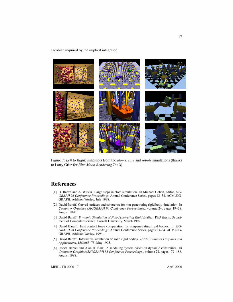
5 ResultsWe now describe the results of simulating four different systems with a timewarp rigidbody simulator (Figures 1 and 7). Our implementation draws from a myriad of com-ponent algorithms and techniques described in the literature; Appendix A describesthe major ones. Robustness—always an issue in rigid body simulation—is paramountfor the kinds of simulations studied here. Anything that can go wrong certainly willwhen simulating large systems over long times. Our implementation favors robustnessover efficiency. The issues are not the underlying components nor the absolute effi-ciency of this particular implementation but the degree to which timewarp improvesany implementation’s performance.

Atoms simulates 200 spheres and 100 water-like molecules bouncing in a dividedbox. During the simulation the divider compresses one compartment and lifts to allowthe gasses to mix. Cars simulates four multibody vehicles with active wheel veloc-ity and steering angle controllers. These drive over a course with speed bumps andan array of 400 spherical pendulums. Robots simulates 20 eight-link manipulatorsthat repeatedly pick up boxes and throw them. The robots are fully dynamic objects,controlled via joint torques commanded by callback functions. Callbacks also use aninverse kinematic model for motion planning. Finally avalanche simulates 300 rigidbodies tumbling down a mountainside, creating a vast number of interactions. With theexception of atoms, all simulations use realistic values for length, mass, time and earthgravity. Each was generated from a single run.

5.1 Full Timewarp Simulation DataTable 1 shows data collected over the course of performing the full simulations. Thepercentages in the total integration and rollback columns are with respect to the simu-lation duration. Computation times were measured on an SGI Onyx (200MHz R10000CPU). Integration and rollback intervals of multibodies and groups were weighted bythe number of individual rigid bodies involved. The reason that total integration minusrollback exceeds duration is because of the added integration involved in localizing dis-continuities. When a discontinuity is detected over an interval, the simulator must com-pute new states of the relevant bodies in order to localize it. This means re-integrating


14

over certain time intervals, increasing the total integration time.3Worth noting is the amount by which the average integration step exceeds the aver-

age interval between discontinuities. This of course is a key advantage of the timewarpalgorithm: integration of a body does not halt at every discontinuity but only at the oneswhich are relevant to it. The fact that the actual integration steps are 2–16 times largerthan the average interval between discontinuities is especially noteworthy since anysimulation strategy (RD, CA, or timewarp) must check for discontinuities at a muchhigher rate than they actually occur. In our experiments, checks outnumbered actualdiscontinuities by two orders of magnitude. Under RD or CA, all bodies are halted atevery check, although the problem is less severe under RD since collision checks aresynchronized. Table 1 also shows that rollback is a modest cost. Through judicious un-doing, timewarp avoids the large amount of wasted work inherent in RD as the numberof bodies increases.

In several performance measures, the avalanche simulation is an outlier. The slowsimulation speed is not because timewarp is not working. The ratio of average integra-tion step to average time between discontinuities is quite good, and the total integrationper body, while high, is not prohibitive. The main difficulty is the complexity of thecontact groups: over 16,000 groups are formed, some having as many as 64 mov-ing bodies and 217 simultaneous contacts. Simulating an avalanche using particle orposition-based physics may be more practical, but the example shows that timewarpcan handle even extreme cases well.

5.2 Comparative Simulation DataTable 1 suggests the timewarp algorithm is a good idea. Further experiments give amore quantitative measure of the improvement it brings. We added alternate main loopsto the simulator to let it use RD and CA policies instead of timewarp (TW). The RDalgorithm is parameterized by the basic timestep to attempt on each iteration; we usedvalues of 0.001, 0.01, and 1/30 second. All five algorithms were run on a two-secondsegment of an atoms simulation, with the divider stationary in the middle of the box andwith the number of bodies varying from 25 to 200. The upper part of Figure 6 showsthe average integration step taken by the simulator under the various algorithms. Theresults confirm the key problem with CA: as the number of bodies increases the averagetime to the next discontinuity check decreases. As Figure 2 shows, the small steps havea drastic effect on computational cost. RD’s average timestep is not as sensitive tothe number of bodies since it always tries to take a fixed size step forward. TW isalso not sensitive to it since the bodies are decoupled. The lower portion of the figureexposes the problem with RD: wasted work. For a two-second, 200-body simulationand a frame rate timestep, RD integrates each body an average of 30 seconds. This isto be compared with TW’s value of 2.3 seconds and the modest percentages in the totalintegration column of Table 1. CA never integrates more than two seconds per bodysince it uses a one-sided approach to each discontinuity.

Actual execution times shed further light. For 100 atoms, RD-1/30 is the narrow3Baraff cleverly avoids this waste by using internal values of the Runge-Kutta integrator to obtain a

polynomial approximation of the state over an integration step for free [5].


15

0.5

1

5

10

50

100

25 50 75 100 125 150 175 200

milli

seco

nds

number of moving bodies

Average Integration Step

TW

RD (0.001)RD (0.01)RD (1/30)

CA

2

5

10

15

202530

25 50 75 100 125 150 175 200

seco

nds

number of moving bodies

Total Length of Integration Intervals Per Body

TW

RD (0.001)RD (0.01)RD (1/30)

CA

Figure 6: Integration statistics for various atoms simulations.

winner at 0.142 s/frame, while TW was 0.147 s/frame and CA was 1.15 s/frame. By200 atoms, TW is clearly superior at 0.388 s/frame, while RD-0.01, the fastest RDalgorithm, was 2.61 s/frame, and CA was 4.74 s/frame.


16

6 ConclusionTimewarp rigid body simulation is clearly able to simulate larger systems with moreinteractions than traditional synchronized simulation algorithms. The most obvious av-enues for future research involve parallel rigid body simulation. Timewarp simulationhelps pave the way to this goal since the individual bodies are evolved asynchronously.If the algorithm runs on multiple processors, delays due to communication latenciesare handled in the same way as bad predictions of discontinuity times: with minimalrollback.

The simplest way to structure a parallel simulator would be to have one masterprocessor that repeatedly sends integration tasks to a bevy of slave processors. All ofthe global data structures could be kept on the master processor, requiring little changein the algorithms presented here. This could significantly boost performance over theuniprocessor case but suffers from a bottleneck at the master. An egalitarian approachin which bodies are distributed among processors is ultimately more scalable. Impor-tant open questions are how to parcel the bodies among processors and how to balanceworkloads. At odds are the goals of minimizing inter-processor communication bykeeping bodies in the same spatial region on a common processor and minimizing idletime by shifting bodies to idle processors. At any rate some method and strategy for mi-grating the bodies between processors seems appropriate. Rollback probably requiresa full antimessage mechanism since the state graph is likely to be distributed. Otherquestions surround how and where to store data structures like the spatial hash table,which is frequently accessed by all bodies. Events involving multiple bodies might beredundantly stored and processed on multiple processors or on only one of the relevantprocessors. Finally, there are various protocol choices for passing state informationbetween processors. Clearly there are many challenges to building a large simulationfarm. Yet the prospect of rich virtual environments built on a physics-based substrateis adequate motivation to pursue them.

A Implementation DetailsOur system is implemented in C++. All geometries are modeled as convex polyhe-dra or unions thereof. The v-clip algorithm [27] is used for narrow-phase collisiondetection; a hierarchical spatial hash table [26, 29] containing axes-aligned boundingboxes is used for the broad phase. For nearby bodies not in contact, times to impact areestimated from current positions and velocities as in [26], but the predictions are notconservative. Persistent contact is modeled using a penalty force method; spring anddamper constants are specified per body pair. Inspired by [1] we use an implicit inte-grator (4th order Rosenbrock [30]) with a sparse solver [15] to handle stiffness inducedby the penalty method. This is only necessary for contact groups; isolated bodies areintegrated with a 5th order Runge-Kutta integrator [30]. We use a smooth nonlinearfriction law, [34]; static friction is not modeled. Reduced coordi-nates are used for multibodies, with dynamics computed by a generalized Featherstonealgorithm [16] in the isolated case and by the spatial composite-rigid-body algorithm[24] within contact groups. The latter is more suited to generating the acceleration


17

Jacobian required by the implicit integrator.

Figure 7: Left to Right: snapshots from the atoms, cars and robots simulations (thanksto Larry Gritz for Blue Moon Rendering Tools).

References[1] D. Baraff and A. Witkin. Large steps in cloth simulation. In Michael Cohen, editor, SIG-

GRAPH 98 Conference Proceedings, Annual Conference Series, pages 43–54. ACM SIG-GRAPH, Addison Wesley, July 1998.

[2] David Baraff. Curved surfaces and coherence for non-penetrating rigid body simulation. InComputer Graphics (SIGGRAPH 90 Conference Proceedings), volume 24, pages 19–28,August 1990.

[3] David Baraff. Dynamic Simulation of Non-Penetrating Rigid Bodies. PhD thesis, Depart-ment of Computer Science, Cornell University, March 1992.

[4] David Baraff. Fast contact force computation for nonpenetrating rigid bodies. In SIG-GRAPH 94 Conference Proceedings, Annual Conference Series, pages 23–34. ACM SIG-GRAPH, Addison Wesley, 1994.

[5] David Baraff. Interactive simulation of solid rigid bodies. IEEE Computer Graphics andApplications, 15(3):63–75, May 1995.

[6] Ronen Barzel and Alan H. Barr. A modeling system based on dynamic constraints. InComputer Graphics (SIGGRAPH 88 Conference Proceedings), volume 22, pages 179–188,August 1988.


18

[7] J. Basch, L.J. Guibas, and J. Hershberger. Data structures for mobile data. In Proceedingsof 8th Symposium on Discrete Algorithms, 1997. To appear in J. of Algorithms.

[8] Raymond M. Brach. Mechanical Impact Dynamics; Rigid Body Collisions. John Wiley &Sons, Inc., 1991.

[9] David C. Brogan, Ronald A. Metoyer, and Jessica K. Hodgins. Dynamically simulatedcharacters in virtual environments. IEEE Computer Graphics and Applications, 18(5):58–69, September 1998.

[10] Stephen Cameron. Enhancing GJK: Computing minimum penetration distances betweenconvex polyhedra. In Proceedings of International Conference on Robotics and Automa-tion. IEEE, April 1997.

[11] Deborah A. Carlson and Jessica K. Hodgins. Simulation levels of detail for real-timeanimation. In Proceedings of Graphics Interface ’97, pages 1–8, 1997.

[12] Anindya Chatterjee and Andy Ruina. A new algebraic rigid body collision law basedon impulse space considerations. Journal of Applied Mechanics, 65:939–951, December1998.

[13] Stephen Chenney, Jeffrey Ichnowski, and David Forsyth. Dynamics modeling and culling.IEEE Computer Graphics and Applications, 19(2):79–87, March/April 1999.

[14] Jonathan D. Cohen, Ming C. Lin, Dinesh Manocha, and Madhav K. Ponamgi. I-collide:An interactive and exact collision detection system for large-scaled environments. In Sym-posium on Interactive 3D Graphics, pages 189–196. ACM SIGGRAPH, April 1995.

[15] J. Dongarra, A. Lumsdaine, R. Pozo, and K. Remington. A sparse matrix library in c++ forhigh performance architectures. In Proceedings of the Second Object Oriented NumericsConference, pages 214–218, 1992. www.math.nist.gov/iml++.

[16] R. Featherstone. The calculation of robot dynamics using articulated-body inertias. Inter-national Journal of Robotics Research, 2(1):13–30, 1983.

[17] S. Gottschalk, M. C. Lin, and D. Manocha. Obb-tree: A hierarchical structure for rapid in-terference detection. In Holly Rushmeier, editor, SIGGRAPH 96 Conference Proceedings,Annual Conference Series. ACM SIGGRAPH, Addison Wesley, August 1996.

[18] Brian Von Herzen, Alan H. Barr, and Harold R. Zatz. Geometric collisions for time-dependent parametric surfaces. In Computer Graphics (SIGGRAPH 90 Conference Pro-ceedings), pages 39–48, 1990.

[19] Jessica K. Hodgins and Nancy S. Pollard. Adapting simulated behaviors for new characters.In Turner Whitted, editor, SIGGRAPH 97 Conference Proceedings, Annual ConferenceSeries, pages 153–162. ACM SIGGRAPH, Addison Wesley, August 1997.

[20] Jessica K. Hodgins, Wayne L. Wooten, David C. Brogan, and James F. O’Brien. Animatinghuman athletics. In SIGGRAPH 95 Conference Proceedings, Annual Conference Series,pages 71–78. ACM SIGGRAPH, Addison Wesley, 1956.

[21] Philip M. Hubbard. Approximating polyhedra with spheres for time-critical collision de-tection. ACM Transactions on Graphics, 15(3), July 1996.

[22] David R. Jefferson. Virtual time. ACM Transactions on Programming Languages andSystems, 7(3):404–425, July 1985.

[23] V. V. Kamat. A survey of techniques for simulation of dynamic dynamic collision detectionand response. Computer Graphics in India, 17(4):379–385, 1993.

[24] Kathryn W. Lilly. Efficient Dynamic Simulation of Robotic Mechanisms. Kluwer AcademicPublishers, Norwell, 1993.

[25] Victor J. Milenkovic. Position-based physics: Simulating the motion of many highly inter-acting spheres and polyhedra. In Holly Rushmeier, editor, SIGGRAPH 96 Conference Pro-ceedings, Annual Conference Series, pages 129–136. ACM SIGGRAPH, Addison Wesley,August 1996.


19

[26] Brian Mirtich. Impulse-based Dynamic Simulation of Rigid Body Systems. PhD thesis,University of California, Berkeley, December 1996.

[27] Brian Mirtich. V-Clip: fast and robust polyhedral collision detection. ACMTransactions onGraphics, 17(3):177–208, July 1998. Mitsubishi Electric Research Lab Technical ReportTR97–05.

[28] J. Thomas Ngo and Joe Marks. Spacetime constraints revisited. In SIGGRAPH 93 Confer-ence Proceedings, Annual Conference Series, pages 343–350. ACM SIGGRAPH, AddisonWesley, 1993.

[29] M. Overmars. Point location in fat subdivisions. Information Processing Letters, 44:261–265, 1992.

[30] William H. Press, Saul A. Teukolsky, William T. Vetterling, and Brian R. Flannery. Numeri-cal Recipes in C: The Art of Scientific Computing. Cambridge University Press, Cambridge,second edition, 1992.

[31] Edward J. Routh. Elementary Rigid Dynamics. Macmillan, London, 1905.[32] Karl Sims. Evolving virtual creatures. In SIGGRAPH 94 Conference Proceedings, Annual

Conference Series, pages 15–22. ACM SIGGRAPH, Addison Wesley, 1994.[33] John M. Snyder, Adam R. Woodbury, Kurt Fleischer, Bena Currin, and Alan H. Barr. In-

terval methods for multi-point collisions between time-dependent curved surfaces. In SIG-GRAPH 93 Conference Proceedings, Annual Conference Series, pages 321–333. ACMSIGGRAPH, Addison Wesley, 1993.

[34] Peng Song, Peter R. Kraus, Vijay Kumar, and Pierre Dupont. Analysis of rigid bodydynamic models for simulation of systems with frictional contacts. Submitted to ASMEJournal of Applied Mechanics, June 1999.

[35] D.E. Stewart and J.C. Trinkle. An implicit time-stepping scheme for rigid body dynamicswith inelastic collisions and coulomb friction. International Journal of Numerical Methodsin Engineering, 39:2673–2691, 1996.

[36] J.C. Trinkle, J.S. Pang, S. Sudarsky, and G. Lo. On dynamic multi-rigid-body contactproblems with coulomb friction. Zeitschrift fur Angewandte Mathematik und Mechanik,77(4):267–279, 1997.

[37] Andrew Witkin, Michael Gleicher, and William Welch. Interactive dynamics. ComputerGraphics, 24(2):11–22, March 1990.


timewarp rigid body simulation - cs.mcgill.cacarl/rigidbody.pdf · timewarp rigid body simulation...

Documents