efficient simulation of contact between rigid and deformable

MULTIBODY DYNAMICS 2011, ECCOMAS Thematic ConferenceJ.C. Samin, P. Fisette (eds.)

Brussels, Belgium, 4-7 July 2011

EFFICIENT SIMULATION OF CONTACT BETWEEN RIGID ANDDEFORMABLE OBJECTS

Eder Miguel? and Miguel A. Otaduy?

?Modeling and Virtual Reality GroupUniversidad Rey Juan Carlos (URJC Madrid), Tulipán s/n, E-28933, Móstoles, Spain

e-mails: [email protected],[email protected]

Keywords: Contact Simulation, Constraints.

Abstract. Contact coupling between deformable and rigid bodies often induces situationswhere the surfaces of both types of bodies collide over a large area. This situation introducesserious difficulties in LCP-type contact solvers, because a large amount of contact constraintsare inertially coupled through the rigid body. In this paper, we present an algorithm for ef-ficiently simulating contact between rigid and deformable bodies. The solution to the LCPinvolves two steps: building the system matrix, which tends to be large and dense due to thecoupling between the rigid and deformable bodies in contact, and solving the resulting prob-lem. We efficiently handle both steps by reformulating the large LCP and separating constraintsets acting on rigid bodies alone, on deformable bodies alone, and on both rigid and deformablebodies. A modified projected Gauss-Seidel solver handles the partitioned sets of constraints inan efficient manner. We demonstrate our algorithm on several complex and contact-intensivescenarios, such as those involving cloth simulations, or contact between bone and soft-tissue.

1

[email protected]

[email protected]

Eder Miguel and Miguel A. Otaduy

1 INTRODUCTION

Many robotics applications involve modeling contact between rigid and deformable objects.Perhaps, the most prominent example of such contact interactions in robotics is grasping, wherethe soft tissue of the fingers interacts with rigid objects in the environment. Other examplesinclude contact between bones and soft human tissue for biomechanical simulation, rigid anddeformable parts in vehicles, or the interaction between the body and rigid parts around us forergonomics analysis.

The diverse properties of rigid and deformable bodies induce complicated configurationsfrom the point-of-view of contact handling. In particular, in this work, we address problemsinduced by the difference in numbers of degrees of freedom and by the sampling of the contactinterface. This contact interface is typically sampled with a set of contact points (e.g., pairsof face-vertex or edge-edge primitives for triangulated surfaces). When contact takes placebetween a pair of rigid bodies, the rigidity of the objects itself limits the number of contactpoints to a few. When contact takes place between a pair of deformable bodies, on the otherhand, the compliance of the material allows the surfaces to mold to each other, hence the numberof contact points may be high. However, in typical deformable bodies discretized with nodalpositions (e.g., in finite element discretizations) each of the contact points affects only a smallnumber of degrees of freedom.

The contact interface between rigid and deformable bodies introduces the following com-plication. Due to the compliance of the deformable body, the contact interface may present alarge surface area, and therefore a large number of contact points. And due to the kinemat-ics of the rigid body, a few degrees of freedom (i.e., the position and orientation of the rigidbody) may be affected by a large number of contact points. This is a rare situation betweenrigid bodies alone or deformable bodies alone, but happens often upon contact between rigidand deformable bodies. Contact solvers based on the formulation of a linear complementarityproblem (LCP) [8] suffer severe complications when many contact constraints affect a small setof degrees of freedom, as we discuss in Section 3.

In this paper, we present an algorithm for efficiently handling contact between rigid and de-formable bodies in the context of LCP-type solvers. The solution to the LCP involves two steps:(i) building the system matrix, which upon contact between rigid and deformable bodies tendsto be large and dense, and (ii) solving the resulting problem. As described in Section 5, our al-gorithm efficiently handles both steps by reformulating the large LCP and separating constraintsets acting on rigid bodies alone, on deformable bodies alone, and on both rigid and deformablebodies. Then, a novel modified projected Gauss-Seidel solver handles the partitioned sets ofconstraints in an efficient manner. In particular, it exploits low-rank matrix computations in or-der to maximize matrix sparsity, and therefore reduce the total computational cost. As a result,assuming n contact constraints, the cost of formulating the LCP matrix and the cost per-iterationof the LCP solver are reduced from O(n2) to an expected O(n).

We demonstrate our algorithm on several complex and contact-intensive scenarios, such asthose involving cloth simulations, or contact between bone and soft-tissue. Thanks to the im-proved asymptotic complexity of the algorithm, timings for LCP construction and solution areimproved by a factor of up to 14x for the examples we show. Even though we limit the demon-strations to contact between rigid and deformable bodies, our algorithm is also applicable inother situations where a large number of contact constraints affects a low number of degrees offreedom, such as contact between deformable bodies with model reduction [13] or embeddedin low-resolution discretizations [17].

2


2 RELATED WORK

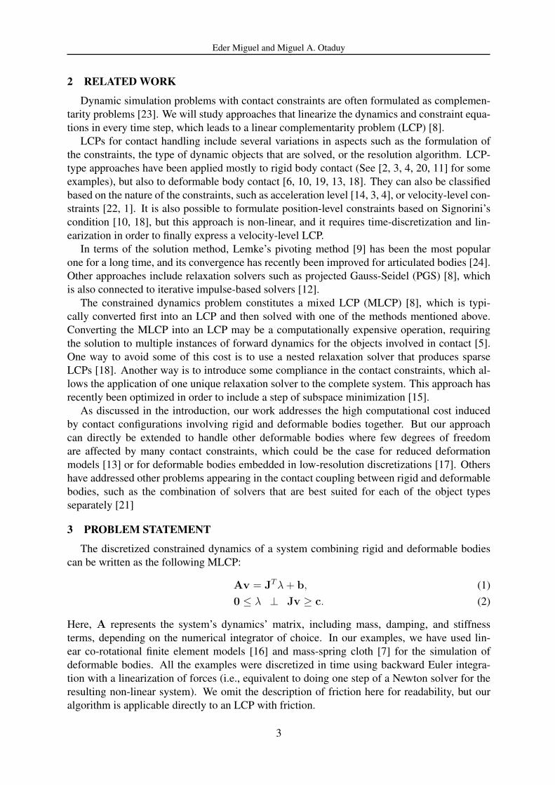
Dynamic simulation problems with contact constraints are often formulated as complemen-tarity problems [23]. We will study approaches that linearize the dynamics and constraint equa-tions in every time step, which leads to a linear complementarity problem (LCP) [8].

LCPs for contact handling include several variations in aspects such as the formulation ofthe constraints, the type of dynamic objects that are solved, or the resolution algorithm. LCP-type approaches have been applied mostly to rigid body contact (See [2, 3, 4, 20, 11] for someexamples), but also to deformable body contact [6, 10, 19, 13, 18]. They can also be classifiedbased on the nature of the constraints, such as acceleration level [14, 3, 4], or velocity-level con-straints [22, 1]. It is also possible to formulate position-level constraints based on Signorini’scondition [10, 18], but this approach is non-linear, and it requires time-discretization and lin-earization in order to finally express a velocity-level LCP.

In terms of the solution method, Lemke’s pivoting method [9] has been the most popularone for a long time, and its convergence has recently been improved for articulated bodies [24].Other approaches include relaxation solvers such as projected Gauss-Seidel (PGS) [8], whichis also connected to iterative impulse-based solvers [12].

The constrained dynamics problem constitutes a mixed LCP (MLCP) [8], which is typi-cally converted first into an LCP and then solved with one of the methods mentioned above.Converting the MLCP into an LCP may be a computationally expensive operation, requiringthe solution to multiple instances of forward dynamics for the objects involved in contact [5].One way to avoid some of this cost is to use a nested relaxation solver that produces sparseLCPs [18]. Another way is to introduce some compliance in the contact constraints, which al-lows the application of one unique relaxation solver to the complete system. This approach hasrecently been optimized in order to include a step of subspace minimization [15].

As discussed in the introduction, our work addresses the high computational cost inducedby contact configurations involving rigid and deformable bodies together. But our approachcan directly be extended to handle other deformable bodies where few degrees of freedomare affected by many contact constraints, which could be the case for reduced deformationmodels [13] or for deformable bodies embedded in low-resolution discretizations [17]. Othershave addressed other problems appearing in the contact coupling between rigid and deformablebodies, such as the combination of solvers that are best suited for each of the object typesseparately [21]

3 PROBLEM STATEMENT

The discretized constrained dynamics of a system combining rigid and deformable bodiescan be written as the following MLCP:

Av = JTλ+ b, (1)0 ≤ λ ⊥ Jv ≥ c. (2)

Here, A represents the system’s dynamics’ matrix, including mass, damping, and stiffnessterms, depending on the numerical integrator of choice. In our examples, we have used lin-ear co-rotational finite element models [16] and mass-spring cloth [7] for the simulation ofdeformable bodies. All the examples were discretized in time using backward Euler integra-tion with a linearization of forces (i.e., equivalent to doing one step of a Newton solver for theresulting non-linear system). We omit the description of friction here for readability, but ouralgorithm is applicable directly to an LCP with friction.

3


0 100 200 300 400 500 600 700 800 900 1000

0

200

400

600

800

1000

nz = 24862 (2.2%)0 20 40 60 80 100 120

0

20

40

60

80

100

120

nz = 8734 (46.5%)0 100 200 300 400

0

100

200

300

400

nz = 33503 (13.6%)

Figure 1: Top row: Snapshots of three different contact situations. Rigid bodies are depicted in red, and deformablebodies (FE meshes with 625 tetrahedra each) in blue. Bottom row: sparsity pattern of the B matrix of the LCP inall three cases. The mixed configuration is dense and large, and it is the target of our algorithm.

The MLCP can be converted into an LCP through Schur complement computation of thematrix A, also named constraint anticipation [5]. We follow an iterative constraint anticipationapproach [18], which solves the MLCP using two nested relaxation solvers. Each iteration ofthe outer relaxation solver formulates an LCP as follows:

0 ≤ λ(i) ⊥ Bλ(i) ≥ d(i), (3)

with B = JD−1A JT ,

and d(i) = c− JD−1A ((LA +UA)v(i− 1) + b) .

A = DA−LA−UA splits matrix A into its (block-)diagonal and the lower and upper triangularmatrices. In the rest of the text, we will drop the subindex i, and we will always refer to oneouter-loop iteration of iterative constraint anticipation.

Fig. 1 shows three different contact situations with rigid and deformable bodies, as wellas the sparsity patterns of matrix B for all three situations. As discussed in the introduction,mixing rigid and deformable bodies produces an LCP that is both large and dense. LCPs withthe same sparsity pattern also appear when the contact forces over the deformable bodies areintegrated explicitly.

Large and dense LCPs imply two negative consequences in terms of computational cost.First, the construction of matrix B has a cost O(n2), with n the number of contact constraints.Since each contact on a rigid body is inertially coupled to all other contacts on the samebody, the formulation of the matrix requires the anticipation of the effect of all pair-wise con-straints [5]. Second, the solution to the LCP using relaxation algorithms requires visiting, foreach row of the matrix, all columns. Then, again, the cost for iterating over the complete matrixbecomes O(n2).

For the sake of completeness, the right-hand-side in Eq. (3) can be formulated with a cost

4


1

a

c

b

2

Figure 2: Schematic decomposition of the bodies and constraints in a contact scenario. Deformable bodies (1) andrigid bodies (2) share a set of constraints (c), while other constraints (a and b) act only on one type of object.

O(n), since it implies sparse matrix - vector multiplications.

4 CONSTRAINT SETS

Even though the LCP matrix B turns out dense and large in situations with contact betweenrigid and deformable bodies, we will show now that it can be split into the sum of a sparse matrixand a dense but low-rank matrix. In the next section, we will take advantage of this separationof the dense low-rank part in order to present an algorithm to formulate and solve the LCP thatis asymptotically (and practically) far more efficient than the straightforward approach.

In order to split the matrix B, we separate the bodies in the scene into two sets:

1. Deformable bodies.

2. Rigid bodies.

Similarly, we separate the contact constraints into three sets:

a. Constraints acting only on deformable bodies.

b. Constraints acting only on rigid bodies.

c. Constraints acting on both deformable and rigid bodies.

Fig. 2 shows the connections between body sets and constraint sets. In a multibody setting,this set decomposition should be carried out for each island of objects.

The previous constraint and object separation allows us to express the matrices and vectorsof the MLCP in Eq. (1) as:

v =

[v1

v2

], A =

[A11 A12

A21 A22

], (4)

λ =

λaλbλc

, J =

Ja1 00 Jb2

Jc1 Jc2

.Given these definitions, the LCP matrix can be expressed as B = Bs +Bd, i.e., the sum of

a sparse matrix Bs and a dense matrix Bd. These matrices are defined as:

Bs =

Ja1D−1A11

JTa1 0 Ja1D

−1A11

JTc1

0 0 0Jc1D

−1A11

JTa1 0 Jc1D

−1A11

JTc1

, and

5


Bd =

0 0 00 Jb2D

−1A22

JTb2 Jb2D

−1A22

JTc2

0 Jc2D−1A22

JTb2 Jc2D

−1A22

JTc2

.The blocks in Bs are built out of the large but (block-)diagonal matrix DA11 , and sparse con-straint Jacobians Ja1 and Jc1. In Bd, on the other hand, the block Jc2D

−1A22

JTc2 is large and

dense, because the constraint Jacobian Jc2 stores values for many contacts acting on just a fewdegrees of freedom (the degrees of freedom of the rigid bodies). However, this same matrixblock Jc2D

−1A22

JTc2 has a low rank, determined by the number of degrees of freedom of the rigid

bodies, independently of the large number of contacts.

5 ALGORITHM

We present now our algorithm for resolving the LCP of contact scenes combining rigid anddeformable objects. This algorithm takes advantage of the low-rank nature of the part of theLCP matrix due to the rigid bodies, Bd. In the context of a projected-Gauss-Seidel (PGS) solver,we iteratively refine the collision response on the rigid bodies, and thus avoid traversing a densematrix in each PGS iteration.

5.1 Rigid Response Refinement

During the resolution of the LCP, we maintain at all times the response velocity of the rigidbodies produced by the current values of the Lagrange multipliers λ. During the jth itera-tion of the PGS solver, after traversing the kth row, let us define as λ(j, k) the temporaryvector of Lagrange multipliers that contains values from the previous and the current itera-tions: λ(j, k) = [λ1(j), . . . λk(j), λk+1(j − 1), . . . λn(j − 1)]. Then, we define the temporaryresponse of the rigid bodies as v2(j, k) = D−1

A22JT2 λ(j, k). We can precompute P = D−1

A22JT2 ,

and then v2(j, k) = Pλ(j, k).When a new row is processed by PGS, the rigid body response can simply be updated as

v2(j, k) = v2(j, k − 1) + Pk(λk(j) − λk(j − 1)), where Pk is the kth column of P. If thescene contains many rigid bodies, Pk is sparse and has non-zero terms only for the rigid bodiesaffected by the kth constraint.

Rigid response refinement allows for inexpensive low-rank updates in the context of the PGSiterations, as we will show next.

5.2 Modified PGS Solver

Given the decomposition of Bs and Bd into diagonal and lower and upper triangular matri-ces, i.e., Bs = Ds − Ls −Us and Bd = Dd − Ld −Ud, an iteration of PGS can be expressedas:

(Ds − Ls +Dd − Ld)λ(j) ≥ d+ (Us +Ud)λ(j − 1). (5)

For the kth row, this can be written as:

(Ds,k − Ls,k +Dd,k − Ld,k)λ(j) ≥ (6)dk + (Us,k +Ud,k)λ(j − 1).

Based on the definition of the temporary vector of Lagrange multipliers, λ, we can rewrite thisexpression:

(Ds,k − Ls,k +Dd,k)λ(j) ≥ (7)

dk + (Dd,k +Us,k)λ(j − 1)−Bd,kλ(j, k − 1).

6


In this expression, the matrix on the left-hand side is sparse, while the dense matrix Bd

on the right-hand side is multiplying a vector of known Lagrange multipliers. Hence, we canexploit the low-rank definition of Bd in order to compute the right-hand side of the inequality.In particular, we apply the concept of rigid response refinement described above:

J2,kv2(j, k − 1) = Bd,kλ(j, k − 1) (8)

so that then:

(Ds,k +Dd,k)λ(j) ≥ dk + Ls,kλ(j)+ (9)(Dd,k +Us,k)λ(j − 1)− J2,kv2(j, k − 1).

This final expression lends itself to an efficient implementation. The modified PGS solverrequiresO(1) computational cost per row, hence a totalO(n) per iteration. Moreover, the matrixBd no longer needs to be computed, hence the cost for building the LCP matrix is also reducedto O(n). This asymptotic cost analysis is verified with the data from our experiments.

The algorithm for each iteration j of the LCP solver can be summarized as follows:

For each constraint kCompute the right-hand side rk in Eq. (9).Compute λ∗k = rk/(Ds,kk +Dd,kk).Project λk(j) = max(λ∗k, 0) .Update v2(j, k) = v2(j, k − 1) +Pk(λk(j)− λk(j − 1)).

The handling of friction using a pyramid approximation of Coulomb’s model can be donesimilarly in the context of the PGS solver, with a block-matrix implementation. Then, theiteration for each constraint requires the computation of a Lagrange multiplier λk in the normaldirection, and two additional values for the tangential directions. Some examples of such solverswith friction are given in [10, 18]. Another possibility is to use staggered projections for normaland friction response [13].

6 RESULTS

We have evaluated the performance of the algorithm in practice on two examples that com-bine rigid and deformable bodies. One example consists of two rigid vertebrae squeezing adeformable intervertebral disk (Fig. 3). The other example shows a piece of cloth that knocksdown a rigid bunny model (Fig. 5). Both examples were tested on an Intel Core 2 Duo 2.3GHz-processor laptop with 3GB of memory.

Fig. 4 compares the timings between our algorithm and the standard approach for buildingthe LCP system and for solving one iteration of the LCP, in the vertebrae example. The timingsare plotted against the number of contact constraints in the scenario, which allows us to validateour asymptotic cost analysis. Both the construction and solution costs show a clear linear trendusing our algorithm. With the standard algorithm, on the other hand, they show a quadratictrend for almost the first half of the contacts. Then, this trend becomes linear. The reason is thatthe quadratic trend is only present until the number of contacts reaches the maximum number ofcontacts suffered by a single rigid body. For higher numbers of contacts, these are split amongrigid bodies, hence the cost is dominated by the linear trend. Nevertheless, the factor of thislinear trend is higher with the standard algorithm than with ours.

7


Figure 3: An intervertebral disk being squeezed between two vertebrae. The vertebrae are simulated as rigidbodies, while the disk is simulated using FEM, with a 6021-tetrahedra mesh. The surface meshes contain 5888triangles for each vertebra, and 8192 for the disk.

0 50 100 150 200 250 300 350 400

2

4

6

8

10

12

14

16

18

Number of Contacts

LCP Construction Cost (in ms.)

standard algorithm

our algorithm

0 50 100 150 200 250 300 350 4000

0.1

0.2

0.3

0.4

0.5

0.6

0.7

Number of Contacts

LCP Solution Cost per Iteration (in ms.)

standard algorithm

our algorithm

Figure 4: Evaluation of the LCP construction and solution cost Vs. the number of contacts in the vertebrae scenario.

Fig. 6 compares as well the construction and solution cost of the LCP, for the bunny example.In this case, the timings are plotted against the simulation steps. Our algorithm outperforms thestandard approach for building and solving the LCP by a factor of up to 14x. The main practicalconsequence of this speed-up is that the examples shown here run at close to interactive rates.

7 DISCUSSION AND FUTURE WORK

The results of our tests demonstrate that our algorithm for simulating contact between rigidand deformable bodies effectively enjoys a linear cost for constructing the LCP system and forsolving one iteration of PGS. Compared to the quadratic cost of the standard algorithm, thisdifference provides important speed-ups that allow for interactive simulations under moderatescene complexity.

The key contribution that leads to the reduced cost is a decomposition of the system matrixinto a sparse submatrix and a dense but low-rank submatrix. Taking advantage of the low-ranknature of the second submatrix, we have designed a modified version of the projected- Gauss-Seidel solver that avoids formulating large and dense matrices. As shown in the paper, ouralgorithm is simple to formulate, and brings little implementation overhead in comparison withstandard PGS solvers for LCPs.

Despite the speed-ups provided by our algorithm, there are still some limitations and openissues. As already mentioned, our algorithm relies on a Gauss-Seidel relaxation solver. Such

8


Figure 5: A rigid bunny model is knocked down by a piece of cloth. The cloth is simulated as a mass-spring modelwith 1681 nodes. The surface meshes contain 4000 triangles for the bunny, and 3200 for the piece of cloth.

0 50 100 150 200 250 300 350

10

20

30

40

50

Simulation Frames

LCP Construction Cost (in ms.)

standard algorithm

our algorithm

0 50 100 150 200 250 300 350

0.5

1

1.5

2

2.5

3

3.5

Simulation Frames

LCP Solution Cost per Iteration (in ms.)

standard algorithm

our algorithm

Figure 6: Evaluation of the LCP construction and solution cost during the course of the simulation in the bunnyscenario.

relaxation solvers may suffer from slow convergence, and we did indeed experience slow con-vergence in some contact situations when large surfaces collided in violent impacts, or when thedeformable bodies suffered a large strain during contact. We plan to evaluate approaches thataddress the slow convergence of relaxation solvers for LCPs [15], and investigate the integrationof our algorithm for efficiently handling contact between rigid and deformable bodies.

Currently, we are applying our approach only to rigid bodies in contact with densely dis-cretized deformable bodies (FE meshes or mass-spring models), but the key concepts presentedhere can be applied in general to any dynamic model where a large number of contacts affect asmall number of degrees of freedom.

Acknowledgments

Eder Miguel was supported by a fellowship from La Caixa. We would also like to thank JaviS. Zurdo for help with demos, Alvaro Pérez for help with renders, and the rest of the GMRVgroup at URJC Madrid.

REFERENCES

[1] M. Anitescu and F. A. Potra. Formulating dynamic multi-rigid-body contact problemswith friction as solvable linear complementarity problems. Journal Nonlinear Dynamics,14(3):231–247, 1997.

9


[2] D. Baraff. Analytical methods for dynamic simulation of non-penetrating rigid bodies. InComputer Graphics (Proceedings of SIGGRAPH 89), pages 223–232, July 1989.

[3] D. Baraff. Coping with friction for non-penetrating rigid body simulation. In ComputerGraphics (Proceedings of SIGGRAPH 91), pages 31–40, July 1991.

[4] D. Baraff. Fast contact force computation for nonpenetrating rigid bodies. Proc. of ACMSIGGRAPH, 1994.

[5] D. Baraff. Linear-time dynamics using Lagrange multipliers. Proc. of ACM SIGGRAPH,1996.

[6] D. Baraff and A. P. Witkin. Dynamic simulation of non-penetrating flexible bodies. Proc.of ACM SIGGRAPH, 1992.

[7] R. Bridson, R. Fedkiw, and J. Anderson. Robust treatment of collisions, contact andfriction for cloth animation. Proc. of ACM SIGGRAPH, 2002.

[8] R. Cottle, J. Pang, and R. Stone. The Linear Complementarity Problem. Academic Press,1992.

[9] R. W. Cottle and G. B. Dantzig. Complementarity pivot theory of mathematical program-ming. Journal of Linear Algebra and Applications, 1, 1968.

[10] C. Duriez, F. Dubois, A. Kheddar, and C. Andriot. Realistic haptic rendering of interactingdeformable objects in virtual environments. Proc. of IEEE TVCG, 12(1), 2006.

[11] K. Erleben. Velocity-based shock propagation for multibody dynamics animation. ACMTrans. on Graphics, 26(2), 2007.

[12] E. Guendelman, R. Bridson, and R. Fedkiw. Nonconvex rigid bodies with stacking. Proc.of ACM SIGGRAPH, 2003.

[13] D. M. Kaufman, S. Sueda, D. L. James, and D. K. Pai. Staggered projections for frictionalcontact in multibody systems. Proc. of ACM SIGGRAPH Asia, 2008.

[14] P. Lotstedt. Numerical simulation of time-dependent contact and friction problems in rigidbody mechanics. SIAM Journal on Scientific and Statistical Computing, 5(2):370–393,1984.

[15] J. L. Morales, J. Nocedal, and M. Smelyansiy. An algorithm for the fast solution ofsymmetric linear complementarity problems. Numerische Mathematik, 111(2), 2008.

[16] M. Müller and M. Gross. Interactive virtual materials. Proc. of Graphics Interface, 2004.

[17] M. Nesme, P. G. Kry, L. Jerábková, and F. Faure. Preserving topology and elasticity forembedded deformable models. ACM Transactions on Graphics, 28(3):52:1–52:9, July2009.

[18] M. A. Otaduy, R. Tamstorf, D. Steinemann, and M. Gross. Implicit contact handling fordeformable objects. Computer Graphics Forum, 28(2):559–568, Apr. 2009.

10


[19] L. Raghupathi and F. Faure. QP-Collide: A new approach to collision treatment. FrenchWorking Group on Animation and Simulation (GTAS), 2006.

[20] S. Redon, A. Kheddar, and S. Coquillart. Gauss’ least constraints principle and rigid bodysimulations. Proc. of ICRA, 2002.

[21] T. Shinar, C. Schroeder, and R. Fedkiw. Two-way coupling of rigid and deformable bodies.Proc. of ACM SIGGRAPH/Eurographics Symposium on Computer Animation, 2008.

[22] D. E. Stewart and J. C. Trinkle. An implicit time-stepping scheme for rigid body dynamicswith inelastic collsions and Coulomb friction. International Journal of Numerical Methodsin Engineering, 39, 1996.

[23] P. Wriggers. Computational Contact Mechanics. Wiley, 2002.

[24] K. Yamane and Y. Nakamura. A numerically robust LCP solver for simulating articulatedrigid bodies in contact. Robotics: Science and Systems, 2008.

11

efficient simulation of contact between rigid and deformable

Documents