Time Varying Equilibrium Real Rates andMonetary Policy Analysis∗

Bharat Trehan and Tao Wu†

Federal Reserve Bank of San Francisco

Revised June 2004

Abstract

Although it is generally recognized that the equilibrium real interest rate(ERR) varies over time, most recent work on policy analysis has been carried outunder the assumption that this rate is constant. We show how this assumptioncan affect inferences about the conduct of policy in two different areas. First, ifthe ERR moves in the same direction as the trend growth rate (as is suggestedby theory), the probability that an unperceived change in trend growth willlead to a substantial change in inflation is noticeably lower than is suggested byrecent analyses (of inflation in the 1970s, for example) that assume a constantERR. Second, if the monetary authority targets a time varying ERR but theeconometrician assumes otherwise, estimated policy rules will tend to exaggeratethe degree of interest rate smoothing as well as the weight that the monetaryauthority places upon inflation.

JEL Classification: E52

∗We would like to thank Kevin Lansing and Glenn Rudebusch for helpful comments as well as MikeAtkinson for outstanding research assistance. The views expressed in this paper do not necessarilyreflect those of the Federal Reserve Bank of San Francisco or the Federal Reserve System.

† Address for Correspondence: Economic Research, Mail Stop 1130, Federal Reserve Bank of SanFrancisco, 101 Market St, CA 94105, USA. Email: Bharat.Trehan@sf.frb.org, Tao.Wu@sf.frb.org.

1 Introduction

The Taylor rule provides a benchmark for monetary policy in terms of three ar-

guments: the equilibrium real interest rate, the output gap and the inflation rate.

Despite its apparent simplicity, it turns out to describe recent monetary policy in

the U.S. rather well. It has also been used extensively to analyze the conduct of

policy, both in the U.S. and abroad.1 However, nearly all the empirical analyses that

we are aware of have been carried out under the assumption that the equilibrium

real rate (ERR) is constant. One exception is the recent paper by Laubach and

Williams (2003), who estimate a model in which the “natural” rate of interest varies

over time and show that mismeasurement of this rate can lead to a deterioration in

the performance of stabilization policy. In this paper we use their framework (with

small modifications) to examine the sensitivity of inferences about monetary policy

to assumptions about the ERR.

We show how this assumption matters in two different areas. First, we show how

a shifting equilibrium rate can affect inferences about episodes that are sometimes

labeled “policy mistakes.” In a well known paper, Orphanides (2003, p. 636) states

that “The bulk of the error [leading to the ‘Great Inflation’ of the 1970s] can be

traced to the mismeasurement of potential output. Examination of the evolution

of estimates of potential output and resulting assessments of the output gap during

the 1960s and 1970s suggests that the problem could be attributed in large part to

the productivity slowdown which, though clearly seen in the data with the benefit

of hindsight, was virtually impossible to ascertain in real time.” Lansing (2002a)

examines this argument as well. In this paper we show that such arguments are

harder to make once one takes into account the fact that the ERR varies over time

and, in particular, that it responds positively to changes in the trend growth rate

of output. Because of this relationship, slower trend output growth is accompanied

by a lower equilibrium interest rate, so that a policy authority which takes a while

to recognize that the growth rate of output has slowed down will also take a while

to recognize that the equilibrium interest rate has fallen. Thus, policy will, in fact,

not be as stimulative as would be suggested by analyses that ignore the link between

1See, for instance, the volume by Taylor (1999).

1

trend output growth and the ERR, and inflation will not rise as much.

To illustrate our argument, we present the results from a simulation where, fol-

lowing a reduction in trend output, a monetary authority that bases policy on a

Taylor rule with a time varying ERR and filters the data using the correct model of

the economy (but does not know about the trend change) generates almost the same

amount of inflation as an authority that knows about the trend change. When the

exercise is repeated under the usual assumption that the ERR is a constant equal to

the observed sample average real interest rate the outcome is a higher inflation rate.

Even this increase in inflation is not strikingly large; to get noticeably large increases

in the inflation rate, we also have to artificially restrict the speed at which the mone-

tary authority learns about the economy. Our conclusion is that —once time varying

ERRs are allowed for— it is not easy to generate significant changes in the inflation

rate as the consequence of a mistake about the trend growth rate using Taylor rules

and the kind of models used here and in much of the literature. This analysis also

applies to the argument recently put forward by Orphanides and Williams (2002),

who ignore time variation in the ERR and argue that the fact that inflation did not

fall noticeably when productivity accelerated in the 1990s suggests that the Fed may

no longer be using rules that depend upon the level of the (unemployment) gap.

Second, we examine what happens to estimates of policy reaction functions in a

situation where the monetary authority targets a time varying ERR. If the econo-

metrician ignores time variation in this rate, estimates of two of the three coefficients

in a simple policy rule are biased upwards. One of these is the coefficient on the

lagged interest rate term; since the size of the lagged interest rate term is generally

interpreted as a measure of the extent of interest rate smoothing (see Clarida, Gali

and Gertler (1999)) this bias will tend to exaggerate the extent to which the policy

authority smooths interest rates. The coefficient on the inflation term is biased up-

wards as well, and this will make the econometrician overestimate the importance

that the authority attaches to controlling inflation. While omitted variable bias ac-

counts for the distortion of the coefficient on the lagged interest rate, the distortion

of the inflation coefficient reflects the effects of the monetary authority’s filtering the

data to recover an estimate of the ERR. This bias affects the coefficient on the out-

put gap as well, but is offset by the fact that the econometrician does not have the

2

policymaker’s measure of the output gap.

We also discuss two ways of getting around these problems: either by including

an ex post measure of the ERR in the estimated reaction function or by allowing for

a serially correlated error term, as recommended by English, Nelson and Sack (2003).

Either method can eliminate the bias in the interest rate coefficient but neither is

completely successful in doing so for the inflation coefficient. Even so, the latter

method seems preferable because it requires less information than the former.

2 The Model

The equilibrium real interest rate is estimated using a model that is quite similar to

Laubach and Williams (2003). The dynamics of the output gap and inflation rate

are described by the following backward-looking equations:

eyt = ay1eyt−1 + ay2eyt−2 + ar2

2Xi=1

(rt−i − r∗t−i) + ε1t (1)

πt =8X

i=1

bπiπt−i + byeyt−1 + bx1x1t−1 + bx2x2t−1 + ε2t (2)

The output gap eyt is defined aseyt = yt − y∗t

where yt and y∗t are the logarithms of actual and potential real GDP in quarter t,

respectively. πt denotes the quarterly changes in the core Consumer Price Index

(CPI). Inflation is modeled as a very persistent process with8P

i=1bπi = 1

2 rt is the

ex-ante real federal funds rate, defined as the difference between the nominal federal

funds rate Rt and the expected inflation rate of next period:

rt = it −Etπt+1

r∗t denotes the equilibrium real interest rate. x1t and x2t are two exogeneous variables

measuring the inflation rate of imported goods and services relative to changes in the

core Personal Consumption Expenditure (PCE) price index and changes in the price

2For parsimony, we restrict the last four coefficients on lagged inflation to be the same, followingGordon (1998) and Laubach and Williams (2003).

3

of crude petroleum relative to that of all crude materials included in the Producers’

Price Index (PPI), respectively. Thus, the output gap is modeled as a function of its

own lagged values and lagged deviations of the real funds rate from the equilibrium

real funds rate. Inflation depends upon its own lags and the lagged output gap, as

well as oil and import prices.

The unobservable equilibrium real interest rate r∗t is assumed to evolve as follows:

r∗t = cgt + dft + zt (3)

zt =3X

i=1

ρizt−i + ε3t (4)

y∗t = y∗t−1 + 0.25gt (5)

gt = gt−1 + ε4t (6)

where gt is the annualized trend growth rate of real GDP and ft is the ratio of the

full-employment fiscal surplus to smoothed total domestic nonfinancial borrowing.3

zt represents the remaining influences on the equilibrium real rate, such as the house-

hold time preference rate and the population growth rate, which we do not model

separately. We assume that zt is a very persistent process, with3P

i=1ρi = 1 in (4)

4.

Laubach and Williams (2003) also assume an additional random shock to the

level of potential output y∗t , so that y∗t is subject not only to changes in the potential

growth rate but also to one-time shifts in level. It turns out to be quite difficult to

distinguish these one-time shifts in the level from changes in the growth rate, because

of which we decided against introducing level shifts. This significantly simplifies the

model estimation, as by doing so we avoid the so called “pile-up problem” discussed

in Stock (1994).

3An alternative is to use potential real GDP to scale the fiscal surplus. However, the debt-GDP ratio has increased quite noticeably over our sample period without any obvious disruption infinancial markets. Since this may reflect the effects of financial innovation over this period, it seemedto us that government deficits relative to the size of the market would provide a better measure of“crowding out.”

4The null that the population growth rate process contains a unit root cannot be rejected at the5% level in our sample.

4

As shown in the appendix, the state-space representation of the model becomes

Yt = A0Xt +H 0St +wt (7)

and

St = FSt−1 + vt (8)

where equation (7) is the observation equation and (8) is the state equation of the

Kalman filter, and

Yt = (yt, πt)0, St = (y

∗t , y

∗t−1, y

∗t−2, y

∗t−3, zt, zt−1, zt−2)

0;

Xt = (yt−1, yt−2, it−1, it−2, πt−1,πt−2, ..., πt−9, x1,t−1, x2,t−1, x1,t−2, x2,t−2, ft−1, ft−2)0

The model is estimated using quarterly U.S. data over the 1965:1 2001:4 period,

and the estimates are shown below.

Table A: Parameter Estimatesay1 1.18 (0.08) c 0.79 (0.31) ar -0.07 (0.03)

ay1 + ay2 0.90 (0.03) d -0.10 (0.001) σ1(ey) 0.78 (0.23)bπ1 0.02 (0.003) by 0.28 (0.08) σ2(π) 1.73 (0.35)bπ2 0.68 (0.09) bx1 -0.01 (0.003) σ3(z) 0.14 (0.03)bπ3 0.30 (0.09) bx2 0.13 (0.02) σ4(g) 0.18 (0.05)

Note: Standard errors are indicated in parentheses.

As can be seen, the coefficients are all statistically significant. Further, the esti-

mated coefficients for the output gap equation (equation 1) are close to the estimates

obtained by others for similar models. Laubach and Williams (2003), for instance,

obtain a value of 0.94 forP

ayi and -0.10 for ar while the comparable coefficients

in Rudebusch and Svensson (1999) are 0.91 and -0.10. However, our estimate of by

(in equation 2) is about twice as large as that obtained by Rudebusch and Svensson,

so inflation is more sensitive to the output gap in our specification. Also, our es-

timate of c = 0.79 (in equation 3) is a little smaller than the comparable Laubach

and William estimate of 1.07, which means that the equilibrium interest rate is not

as sensitive to the trend growth rate in our specification as it is in their’s.5 Finally,

5Coefficient values from the Laubach-Williams paper are from their baseline case (where zt followsa random walk). See Table 1 in their paper.

5

note that the sign of d (also in equation 3) is consistent with “crowding out,” that

is to say a decrease in the fiscal surplus (or an increase in the deficit) leads to an

increase in the equilibrium real interest rate.

3 Policy Analysis

This section studies the role of the time-varying equilibrium real interest rate in

monetary policy analysis. We examine two issues. First, we look at how allowing for

a time-varying equilibrium real interest rate affects inferences regarding the conduct

of policy when there is a shift in the trend growth of real GDP. Second, we look

at what happens to the estimates of a monetary policy reaction function when the

econometrician mistakenly assumes a constant equilibrium real interest rate.

We assume that monetary policymakers set rates according to the well known

“Taylor rule,” in which the level of the nominal interest rate depends on the equi-

librium real interest rate, the output gap and inflation. While the precise form of

the rule we employ below varies depending on the issues under consideration, the

benchmark specification is given by

it = Etr∗t + π̂t + αeyt + β(π̂t − π) (9)

where π̂ denotes the four quarter average of the inflation rate and π denotes the

inflation target of the monetary authority. According to this rule, the monetary

authority moves the real rate above its equilibrium value if output is above trend or

if the inflation rate is above its target rate. Note that the rule does not contain a

lagged value of the nominal interest rate on the right hand side.

3.1 Changes in the trend growth rate: the 1970s and the 1990s

The link between trend growth rates and the equilbrium real rate of interest can

complicate the task of analysing policy during periods when there is a shift in trend

growth rates. Consider, for instance, the argument put forward by Orphanides

(1999) and also examined by Lansing (2002a). Orphanides argues that because the

Fed did not realize that the trend growth rate had slowed during the 1970s it followed

6

a monetary policy that was too stimulative, thereby causing inflation to accelerate.6

However, both analyses are based on the assumption of a constant real rate. In

this section, we show that such an argument is harder to make if the analysis allows

for a time varying interest rate. Essentially, our argument is that if the monetary

authority misses the downward shift in the trend growth rate of output it is also

going to miss the accompanying decline in the ERR (since the ERR and the trend

growth rate are positively correlated from (3) above), and that these two errors will

offset each other to some extent. A similar logic applies to some monetary policy

analyses of the 1990s. For instance, in their discussion of monetary policy in the

1990s, Orphanides and Williams (2002) argue that if the Fed had been following a

Taylor rule during this period it would have engineered a deflation because of a delay

in realizing that the trend growth rate had shifted up, and the fact that it did not

generate such a disinflation suggests that it was following a more robust rule.7 Once

again, allowing for a time varying equilibrium real rate makes it harder to justify

such a conclusion.

We illustrate these issues by simulating an episode during which the output trend

rate changes and show how the subsequent behavior of inflation depends upon the

assumed behavior of the ERR. We begin by assuming that the economy is described

by equations (1) to (6), so that the equilibrium rate moves over time. Next, we

assume that the trend growth rate of output (gt in (6) above) decreases by 0.15

percent each quarter over a period of 10 quarters, for a total decrease of 1.5 percent.

Given the estimate that the coefficient c equals 0.8 in equation (3) above, the drop

in gt implies that r∗t will fall by 1.2 percent. The economy is also hit by shocks to

output, inflation and the ERR, which are assumed to be normally distributed with

standard deviations as shown in section 2 above. The inflation target π is assumed

to be 3 percent. We start all simulations at the inflation rate that prevailed at

6 A somewhat different argument is made by Orphanides and Williams (2002), who suggest thatthe high inflation of the 1970s resulted from misperceived increases in both the natural rate ofunemployment and the equilibrium real rate of interest. More specifically, they argue that the ERRrose with the high growth of the 1960s; their estimates of the ERR, however, show a rapid declinein the early 1970s.

7Orphanides and Williams (2003) use a policy rule in which the monetary authority reacts tothe gap between the unemployment rate and the natural rate instead of the gap between actual andpotential output. Their robust rule sets the change in the interest rate as a function of unemploymentand inflation gaps.

7

the end of 1969. Importantly, for our benchmark simulation we assume that agents

know the model structure and use the Kalman filter to learn about the shocks to

the economy. Such assumptions about rational expectations are quite different from

what is assumed in the literature on learning; below, we will discuss what happens

when we relax this assumption.

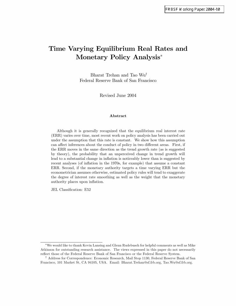
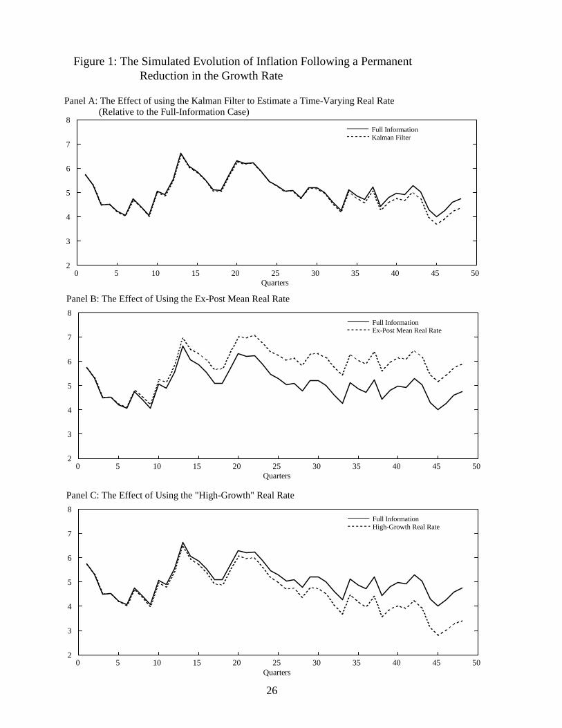
The solid line in panel A of Figure 1 (which is also reproduced in the remain-

ing two panels to facilitate comparison) shows what would happen to inflation if the

policymaker were assumed to know the right model and also to know about all the

shocks hitting the economy (including the change in trend). Note that in the bench-

mark case, the inflation rate at the end of the simulation is a little bit lower than

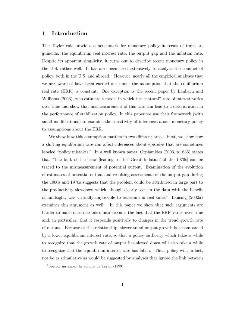
it was at the beginning. The associated ERR is shown in Figure 2 with the label

“actual real rate.” Next we drop the assumption that policymaker knows about the

shocks hitting the system and assume, instead that the policymaker uses the (one-

sided) Kalman filter and the correctly specified model to obtain estimates of these

shocks. The inflation rate (shown as a dashed line in panel A of Figure 1) turns

out to be quite close to the rate generated under the full information case and is,

in fact, slightly lower by the end of the simulation. Essentially, what happens here

is that the effects of the initial over-estimate of the reduced trend growth rate are

offset by the over-estimate of the equilbrium real interest rate (see Figure 2), so that

inflation does not move very far from the full information case. Of course, the almost

exact offset between these two cases is not guaranteed, and the exact outcome will

depend upon the shocks hitting the system, both historically (since these determine

the variances used in the Kalman filter) as well as over the course of the simulation.

For instance, a large increase in the ERR (which occurred at about the same time as,

but was unrelated to, the decrease in trend growth) could lead to an inflation rate

substantially higher than the full-information inflation rate.

Consider next what happens in a simulation where the shocks are the same as

before but where the ERR is assumed to be constant. The value of the constant

equilibrium rate to be used in the Taylor rule (10) is obtained in a way that is similar

to Orphanides (1999) and Lansing(2002a).8 Specifically, this rate is obtained by

8Orphanides uses a value of 2 percent for the equilibrium real rate which he points out is thevalue in Taylor’s original specification and is also close to the 2.2 percent “..average ex post interestrate for the estimation sample.” (See page 12.)

8

taking an average of the expost real rate generated in the simulation, and is shown

in Figure 2 with the label “ex-post mean.” The result of this exercise is an inflation

rate (shown as the dashed line in the middle panel of Figure 1) that begins to exceed

the inflation generated in the “full information” case soon after the downward shift

in the growth rate is complete, and is consistent with the contention that such a

downward shift is likely to lead to an increase in inflation.

The assumption about the ERR turns out to be crucial for this result. Taking

an average of the ex post real rate during a period in which the actual ERR is high

in the early part of the sample but falls later on leads to an estimate that is too low

(relative to the actual rate) early on and too high later in the sample. The resulting

simulation generates an inflation rate that is higher than what the full-information

simulation produces. However, other ways to do a simulation with a fixed ERR

can produce inflation outcomes that are quite different. For instance, consider a

monetary authority that has been operating in a high trend-output-growth regime

for a while and which also believes that the equilibrium interest rate is constant.

It is likely that the (constant) ERR estimate of such an authority will reflect the

high actual equilibrium rates that prevail during this period, and it is unlikely that

this estimate will decline very quickly following an unperceived decline in the trend

growth rate. For instance, if the monetary authority were to follow the practice

of using the average of the expost real rate over the data sample actually at hand

at the time of setting policy as an estimate of the equilibrium rate, a reduction in

the trend growth rate (with the resulting decline in the true ERR) could leave its

estimate of the ERR above the true ERR for an extended period of time. The size

and persistence of this error would, of course, depend upon variables such as the

length of the previous high growth regime as well as the size of the shift in the trend

growth rate. As an extreme example, we show what would happen to the inflation

rate if the monetary authority conducted policy during the low growth period (that

is, during a period in which the trend growth rate had fallen) using an estimate of

the ERR that was fixed at the value attained at the end of the high growth period

(shown as the “High-Growth Real Rate” in Figure 2). In this extreme case, the

inflation rate (shown as the dashed line in Panel C of Figure 1) actually falls below

that generated under the full information assumption. By the end of the simulation

9

the size of the shortfall is about the same as the size of the increase in inflation in

Panel B of the figure.

A noticeable feature of the simulations shown here is that the costs of “policy

mistakes” about the trend growth rate appear to be relatively small. Specifically,

the difference between the inflation rates generated in either of the two simulations

where the ERR is assumed fixed (whether at the sample average or at the beginning-

of-sample value) and the full information case is around 1 to 1-1/2 percent, even

by the end of the simulation. By comparison, studies such as Orphanides (2003)

and Orphanides and Williams (2002) generate noticeably larger costs of such policy

mistakes. Policy mistakes related to trend shifts lead to relatively small costs in

our simulations because the monetary authority can detect these changes relatively

quickly. This in turn is related to the assumptions that the monetary authority

knows the correct structure of the model (except for the nature of the ERR process,

of course) and uses the Kalman filter to recover the values of the shocks hitting the

economy. To demonstrate this we present the results from a simulation in which

the monetary authority learns about changes in the economy rather slowly, an as-

sumption that is similar in spirit to the relatively inertial learning rule that is used

by Orphanides and Williams (2002). Specifically, we alter the variance-covariance

matrix of the shocks so that the it takes the monetary authority twice as long as

before to detect half the cumulative shift in the trend growth rate. The results of

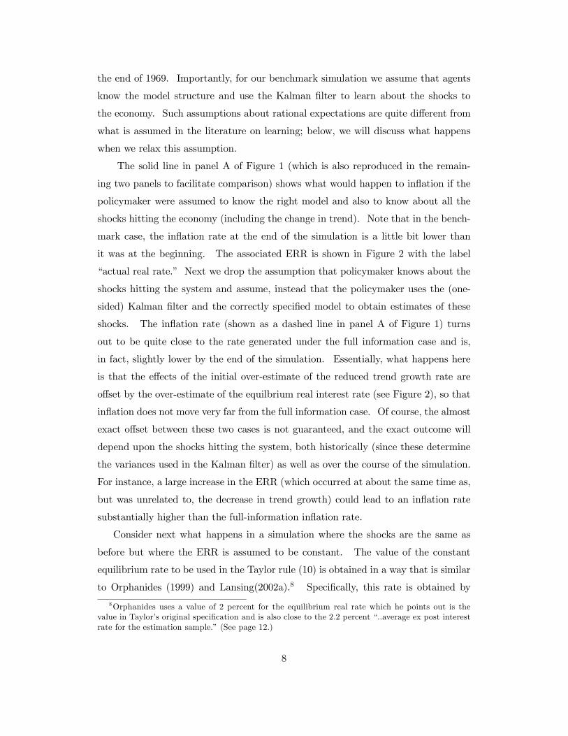
this exercise are shown in Figure 3. Panel A of the figure shows that even with slow

learning inflation does not deviate noticeably from the full information case as long

as the monetary authority is assumed to know the structure of the model. Things

are quite different in the simulation based upon the ex-post average real rate (Panel

B of Figure 3). Now, the inflation rate exceeds inflation under the full information

case by some 4 percent by the end of the simulation.

Our results demonstrate that generating a sustained change in the inflation rate

in response to a change in the trend growth rate is no easy task. Ignorance about the

structure of the model (here about the nature of the ERR) is not enough. As we have

shown, in order to get inflation to go up after a decrease in the trend growth rate (for

example), not only must the authority not know about time variation in the ERR

but it must end up with an estimate of the constant ERR that is “too low.” Such

10

an assumption may be hard to justify when the economy is coming off a high growth

- high interest rate period. And even this is not enough to generate a substantial

increase in inflation out of an empirically plausible shift in the trend growth rate.

For this we have also had to reduce the speed at which the monetary authority learns

about the underlying shocks to the economy. Here it is worth emphasizing that this

last assumption is not sufficient to generate sustained changes in inflation when the

growth trend changes either; we still need to assume that the monetary authority

makes the “right” kind of mistake about the ERR.9

These results also have a bearing on some recent research on robust policy rules.

Specifically, Orphanides and Williams (2002) argue that “..difference rules for mon-

etary policy, in which the short term nominal interest rate is raised in response to

inflation and changes in economic activity” are likely to lead to better economic out-

comes than the more conventional rules which are based on levels (such as (9) above)

because they are less likely to be susceptible to mistakes in measuring natural rates

(or potential growth rates). Our results suggest that because a time varying equi-

librium rate can move to offset the effects of some kinds of shocks, policy rules based

on levels may not always perform as badly (relative to difference rules) as would be

suggested by exercises that ignore this comovement.

3.2 Estimating policy rules

For our second exercise we examine how the existence of a time varying equilibrium

real rate affects the econometrician’s ability to recover the correct coefficients when

estimating policy rules. We begin by asking what happens to estimates of the policy

rule when the econometrician assumes that the equilibrium real rate is constant.

We assume that the monetary authority follows the policy rule specified in equa-

tion (9). However, (for now) we assume that the econometrician believes that the

policymaker sets policy according to one of the following two alternatives, either :

it = κ0 + π̂t + βyeyt + βπ(π̂t − π) (10)

9Another way to generate substantial changes in inflation is to assume a time varying inflationtarget, as in Kozicki and Tinsley (2001, 2003).

11

or

it = (1− γ)(κ0 + π̂t + βyeyt + βπ(π̂t − π)) + γit−1 (11)

In equation (11) the policymaker can be viewed as adjusting gradually to a target

real rate which equals a constant plus a term that depends upon the output gap and

the deviation of the inflation rate from its target value. The policymaker reacts

to the same set of variables in equation (10) but here the adjustment to target is

assumed to be instantaneous. We now consider how the econometrician’s use of one

of these incorrectly specified policy rules can affect inferences about the conduct of

policy.

The econometrician’s assumption of a constant equilibrium rate amounts to omit-

ting the authority’s measure of the ERR in the estimated policy rule. Consider, first,

what happens if the econometrician estimates a policy rule without a lagged interest

rate, specifically equation (10) above. To the extent that the output and inflation

variables are correlated with the authority’s measure of the ERR, the estimated co-

efficients on these variables will be biased, with the direction and extent of the bias

depending on their relationship to the equilibrium rate.10 For instance, an increase in

the true ERR that was not immediately perceived by the monetary authority would

tend to push up the output gap (from equation (1)) as well as inflation (equation

(2)) leading to a positive correlation between the ERR and these variables. Thus,

omitting the equilibrium rate would tend to bias the coefficients on these variables

upwards. By contrast, a positive shock to the trend growth rate would tend to induce

a negative correlation and a downward bias to the coefficient on the inflation variable

in an equation such as (10). Thus, whether the estimated coefficient turns out to

be larger or smaller than the true coefficient will depend upon the shocks hitting the

system and the kind of correlation that they induce between different variables.

Consider now what happens if the econometrician estimates a rule that includes

a lagged interest rate term, that is to say, equation (11) above. It is easy to see that

the estimate of γ will tend to be significant if there is serial correlation in Etr∗t even

10For each of the variables included in the regression, the omitted variable bias equals the coefficientof the omitted variable in the correctly specified regression multiplied by the coefficient of the includedvariable in a regression where the omitted variable is regressed on all the included variables. SeeGreene(2000) for a discussion.

12

if the monetary authority pays no attention to it−1, for the lagged interest rate will

act as a proxy for the omitted (estimate of the) ERR. In the empirical literature

the finding of a non-zero coefficient on it−1 is pretty much universal and is generally

interpreted as evidence that the monetary authority adjusts interest rates gradually,

that is, it “smooths” interest rates. Over the years, a number of theories have been

proposed to motivate this behavior.11 The argument presented here is different,

in as much as we argue that the coefficient on the lagged interest rate term is also

affected by factors other than interest rate smoothing, and is related to arguments

put forward by Rudebusch (2002) and Lansing (2002a). Rudebusch (2002) argues

that monetary policy rules that allow for gradual adjustment are misspecified, and

that the lagged interest rate actually reflects serially correlated shocks to the policy

rule. Lansing (2002a) shows that the use of a output gap measure based on “full

sample” information (that is, information that was not available to the authority at

the time that policy decisions were made) when estimating policy reaction functions

tends to increase the coefficient on the lagged interest rate term, thereby leading to

the illusion of interest rate smoothing.

Inclusion of the proxy variable it−1 also alters the coefficients of the remaining

variables (that is, it will cause the estimated values of βy and βπ in (10) to be

different from those in (11)), with the exact change depending upon a number of

factors. The change in coefficients could be an improvement under certain conditions;

for instance if it−1 and Etr∗t were highly correlated and if the component of it−1 which

was orthogonal to Etr∗t was also orthogonal to the other variables and the error term

in the estimated equation. Alternatively, if this component was large and correlated

with the other variables or the error term in the estimated equation inclusion of the

lagged interest rate could move the estimates of βy and βπ further away from their

true values.12

What happens when the econometrician does include a measure of the ERR in the

estimated policy rule? While this is likely to make the estimated coefficients more

accurate, it is unlikely to eliminate the bias entirely. As the discussion of omitted

variable bias above indicates, the monetary authority generates nonzero correlations

11See, for instance, Barro(1989), Cukierman(1991), Goodfriend(1991), Woodford(1999). See alsoSacks and Wieland(2000) for a more general discussion.12See Maddala (1977) for a discussion.

13

between the estimate of the ERR that it uses in the policy rule and either inflation

or the output gap when it filters the data to determine the true state of the economy.

The implication is that it will be impossible to completely eliminate this bias unless

the econometrician were to come up with the exact measure of the ERR used by the

monetary authority. This problem is similar to the one that arises because the econo-

metrician does not know the value of the gap that is used by the monetary authority

and that has been discussed by Lansing (2003), Orphanides (2002) and Rudebusch

(2001). One reason the consequences will be different is that the econometrician is

likely to impose a coefficient of 1 on the ERR, so measurement problems will show

up in the other coefficients of the policy rule.

3.2.1 Estimating a Mis-Specified Rule

We examine these issues by undertaking sets of simulations that differ in what the

policymaker and the econometrician are assumed to know about the economy. The

benchmark case is one where we assume that the policymaker knows the model spec-

ification, the coefficient values as well as all the shocks hitting the system. Policy is

given by (9); thus, the policymaker does not smooth interest rates. By contrast, the

econometrician assumes that the ERR is constant; consequently, we assume that she

uses modified versions of equations (1) and (2). Specifically, we assume that the

econometrician uses versions of these equations which do not contain r∗t , but whose

coefficients are exactly the same as those shown above. In addition, the econome-

trician also knows equations (5) and (6). These assumptions allow us to focus upon

the effects of the econometrician’s mistake about the ERR.

Each simulation consists of 140 draws (to mimic quarterly data over a 35 year

sample) of four zero-mean, normally-distributed shocks, whose standard deviations

are obtained from the estimation of the model. Thus, at each point in time, the

system is hit by a set of 4 shocks that determine the values of the variables that the

policy authority can observe: yt and πt. In our benchmark case the authority can

see these shocks and so is able to compute the correct values of the output gap and

the ERR for use in (9). Next period, the entire exercise is repeated. After the

simulation is complete, that is, we have generated data for the entire period under

study, we filter the data under some alternative assumptions and estimate the two

14

alternative versions of the policy rule equations (10) and (11). We then record the

estimates of βy, βπ and γ obtained from this exercise. We repeat this exercise a

thousand times.

The median estimates of the coefficients obtained from this exercise are shown

in the top panel of Table 1, along with the intervals that contain 90 percent of the

estimated values.13 Here we assume that the econometrician knows the gap used by

the monetary authority when setting the interest rate, which in Case I is also the true

output gap. The first column (A1) shows that the econometrician will recover the

true coefficients of the reaction function when no lagged interest rate term is included

in the equation, that is to say when she estimates the policy rule (10). This may

appear surprising at first glance since equation (10) clearly omits a relevant variable:

the equilbrium real rate of interest. It turns out, however, that in the model used

here the ERR is not correlated with either the correctly measured output gap or

the inflation rate, implying that the econometrician can expect to recover unbiased

estimates of the coefficients βy and βπ. Things change once the lagged interest rate

is included in the estimated equation, that is, when the policy rule (11) is estimated.

The median estimates of βy and βπ move away from the true values, reflecting the

fact that the lagged interest rate is correlated with both inflation and the output

gap. And the median estimated value of γ (the coefficient on the lagged interest

rate) turns out to be 0.32 with 90 percent of the estimated values lying between 0.12

and 0.64.

For Case II we drop the assumption that the monetary authority knows the dis-

turbances hitting the economy and assume instead that it too must filter the data to

obtain estimates of the output gap and the ERR. We still maintain the assumption

that the authority knows the true model. Panel A in the lower half of the table

shows what happens when the econometrician knows the measure of the gap used by

the monetary authority. Note that in contrast to Case I above, the econometrician

no longer recovers the true values of βy and βπ even when the lagged interest rate

is not included in the estimated equation. This is because the monetary authority’s

13We ignore the existence of the zero bound in the simulations presented here. Imposing thezero bound increases the size of the 90 percent intervals because of a relatively small number ofsimulations where the interest rate hits the zero bound. It also leads to larger coefficients on thelagged interest rate term.

15

filtering of the data induces positive correlations between its estimates of yt and r∗tas well as πt and its estimate of r∗t . Thus, the omission of the policymaker’s measure

of the ERR leads to an upward bias in the estimated coefficients of inflation and the

output gap. And inclusion of the lagged interest rate actually makes things worse,

as the next column indicates. While the estimate of βπ goes up only slightly, the

median value of βy rises to 0.7 and 90 percent of the time the econometrician recovers

a value of βy that is larger than the true value. The median estimate of γ turns out

to be 0.24.

Panel B (Case II) shows what happens to the estimated policy rule coefficients

when the econometrician no longer has access to the measure of the output gap used

by the monetary authority. The largest change is the drop in the value of βy, a drop

which is consistent with the results reported by Lansing(2002a), among others. Note

that the decline actually moves the estimated value of βy closer to the true value

than it was before. By contrast, the estimate of βπ gets pushed a little further away

from the true value. In fact, each of the changes we consider pushes the estimated

value of βπ further away from the true value. For instance, making the monetary

authority filter the data to obtain estimates of yt and r∗t when the lagged interest rate

is not included in the estimated policy rule raises the estimate of βπ from 0.5 to 0.61

(compare the estimates of βπ in Case I Panel A1 with those in Case II Panel A1),

adding the lagged interest rate term pushes the estimate up to 0.62 (compare the

estimates of βπ in columns A1 and A2 in Case II) and dropping the assumption that

the econometrician has access to the monetary authority’s measure of the output gap

raises the coefficient to 0.67 (Compare the estimates of βπ in columns A2 and B2 in

Case II).

Column B2 also shows that the median estimate of γ is 0.26 percent; it turns

out that the estimate of γ is significant at the 1 percent level in 93.9 percent of the

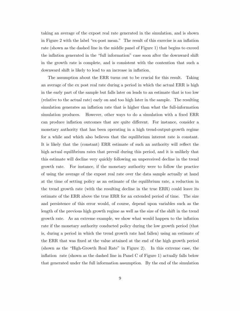
simulations. Finally, to provide a better sense of the distribution of our estimated

coefficients in Case IIB we plot the frequency distributions in figure 4 (panels A

through C). The distributions of βy and γ are noticeably skewed to the right.

For our final exercise we drop the assumption that the monetary authority is

aware of the existence of r∗t . This allows us to generate a set of results that are

comparable to earlier results in the literature—where the policymaker is assumed to

16

target a constant ERR. In this case, both the policymaker and the econometrician

filter the data using the correct version of the Philips curve (that is, equation (2)),

and the mis-specified version of (1), one that assumes that the ERR is a constant.

Another consequence is that policy is set according to

it = κ00 + α byrt + β(π̂t − π) (12)

where byrt denotes the one-sided real-time estimate of the output gap. Not surprisingly,panel A of Case III in Table 1 shows that if the econometrician also knows the value

of the gap used by the monetary authority, she will recover the exact coefficients used

by the monetary authority every time. If the gap must be estimated (panel B), the

median value of βy drops noticeably, with the estimated value lying below the true

value in more than 90 percent of the simulations, whether or not a lagged interest rate

term is included in the equation. If a lagged interest rate term is included (column

B2) it tends to have a small positive coefficient, which turns out to be significant at

the 5 percent level in 56.9% of the simulations.

How sensitive are the results in Table 1 to the assumption that the monetary

authority does not smooth interest rates? To answer this question, we repeated

the entire set of exercises above under the assumption that the true policy reaction

function is given by

it = 0.3it−1 + 0.7(κ1 + 0.5eyt + 0.5π̂t)i.e., the true value of γ = 0.3. The results are shown in Table 2 and turn out to

be not that different from those in Table 1. For instance, if the monetary authority

targets a time varying ERR the estimated coefficient on the lagged interest rate is

biased upward, with the estimated value exceeding the true value in more than 90

percent of the simulations as long as the authority knows the true model.

Implications and Empirical Significance We have shown that the coefficients

that the econometrician recovers are quite sensitive to the what the monetary au-

thority is assumed to know about the structure of the economy. Median values of

βy in Table 1, for instance, range between 0.33 and 0.7, with the true value of 0.5

lying outside the 90 percent range associated with either of these two estimates.

17

The results under the perfect information assumption are clearly unrealistic and

are included only to highlight the role that filtering of the data has upon the estimated

coefficients. As can be seen in either Table 1 or 2, the monetary authority’s filtering

of the data tends to bias upwards the estimates of βy and βπ. The upward bias in the

former disappears when we make the more realistic assumption that the authority’s

measure of the gap is unavailable to the econometrician, which is to say that the

upward bias in βy that is due to filtering is more or less offset by the downward bias

induced by the use of the wrong measure of the output gap. Also the upward bias

in γ, the coefficient on the lagged interest rate, is approximately 0.2, with the exact

value depending upon the assumption one makes about whether or not the authority

actually smooths interest rates.

The results in Case III (in Table 1 or 2) highlight the fact that these issues only

arise in a setup where the monetary authority is targeting a time varying ERR If

the authority ignores this time variation we recover a more familiar set of results (as

in Lansing (2002a)). Specifically, there is no upward bias in the estimate of βπ, but

the econometrician’s inability to obtain the appropriate measure of the output gap

leads to a noticeable downward bias in the estimate of βy and a rather small upward

bias in γ.

How reasonable is it to assume that the monetary authority targets a time varying

ERR? The earliest explicit discussion of this issue that we have come across is in

Chairman Greenspan’s July 1993 testimony to Congress, where he stated that:

“One important guidepost is real interest rates, which have a key bearing on

longer run spending decisions and inflation prospects.

In assessing real rates, the central issue is their relationship to an equilibrium

interest rate, specifically, the level that, if maintained, would keep the economy at

its production potential over time. Rates persisting above that level, history tells

us, tend to be associated with slack, disinflation, and economic stagnation–below

that level with eventual resource bottlenecks and rising inflation, which ultimately

engenders economic contraction. Maintaining the real rate around its equilibrium

level should have a stabilizing effect on the economy, directing production towards

its long-term potential.

The level of the equilibrium real rate–or more appropriately the equilibrium

18

term structure of real rates–cannot be estimated with a great deal of confidence,

though with enough to be useful for monetary policy... Moreover, the equilibrium

rate structure responds to the ebb and flow of underlying forces. So, for example, in

recent years the appropriate real rate structure has doubtless been repressed by the

headwinds of balance sheet restructuring and fiscal retrenchment.”

It seems to us that this is not the first time that the Fed realized that equilibrium

interest rates vary over time. Thus, we are inclined to interpret earlier warnings

by Fed Chairmen about the need to reduce federal budget deficits as expressing a

concern about the tendency of continued deficits to push up equilibrium interest

rates. Empirically, then, we would argue that the results in Case IIB provide a more

realistic measure of the bias in various coefficients of estimated Taylor rules—at least

over the last two decades or so.

To the extent that this is true, the results of our exercise suggest that estimated

policy reaction functions that do not allow for a time varying ERR are likely to have

estimates of βπ that are biased upwards. Any downward bias in βy is not likely

to be very big, as the effects of not knowing the measure of the output gap used

by the monetary authority are likely to be offset by the effects of not knowing the

authority’s measure of the ERR. As for the debate on interest rate smoothing, our

estimates suggest a bias of roughly 0.2, with relatively little of this reflecting the

effects of not knowing the authority’s measure of the output gap. A bias of 0.2 may

not appear to be large, especially in view of the fact that γ is often estimated to be

around 0.8 or 0.9 for postwar U.S. data. However, this difference is large enough

to make a noticeable difference to the implied persistence of the funds rate. For

instance, if γ=0.9 it takes the monetary authority seven quarters to close half the

gap between the actual and desired funds rate, while if γ=0.7 the authority takes

only two quarters to cover roughly the same distance.

3.2.2 Two Alternative Solutions

Finally, we ask what the econometrician can do to recover more accurate values of the

Taylor rule coefficients in a world where the ERR varies over time. If we assume that

she knows the true structure of the model and the correct policy rule the answer is

straightforward: She simply constructs an estimate of the ERR and includes it in the

19

estimated policy rule. With the coefficient on the ERR restricted to 1, Table 3 shows

the coefficient estimates for the remaining variables in the policy rule under different

assumptions about how much the policymaker knows. In the interests of brevity we

only present the results for the cases where the policymaker does not know the shocks

hitting the economy and where the econometrician does not know the policymaker’s

measure of the output gap. Because we set γ = 0 in our simulations, the two cases

in Table 3 are comparable to Table 1. Including the econometrician’s measure of

the ERR leads to an improvements in the estimates of γ while the estimates of βy

are generally worse. The estimates of βπ improve when the authority is assumed to

know the correct model.

The assumption that the econometrician has the right model of the economy

or even the one that is being used by the monetary authority and can use that

to construct an ex post measure of the ERR is obviously one that is unlikely to be

fulfilled in practice. In fact, any estimate of the ERR is likely to be controversial: real

interest rates themselves are unobservable and equilibrium values harder to measure

still.14 Consequently, we also present the results from a technique that does not

require knowledge of the ERR. Specifically, this requires following the suggestion by

English, Nelson and Sacks (2003) to estimate an interest rate equation that allows

for both a lagged interest rate term on the right hand side and autoregressive errors.

To see why this technique might work, note that they recommend estimating the

following equation:

it = (1− γ)bit + γRt−1 + υt (13)

where bit = a0 + aππ̂t + ayyt

and

υt = ρυt−1 + t

A look at (13) shows that estimating this equation is similar to estimating a Taylor

rule with a lagged interest rate and a time varying ERR which is approximated by

the υt term.14For a discussion of the difficulties in estimating equilibrium real rates, see Orphanides and

Williams (2002) as well as Clark and Kozicki (2004).

20

In Table 4 we show the estimates we obtain when this specification is estimated

using the same data as in Table 1 (where it was assumed that the monetary authority

was not smoothing interest rates). For Case II(B) we obtain a median estimate of

γ that is quite close to zero and is noticeably smaller than the comparable estimate

in Table 115. The estimate of βy is quite close to the true value of 0.5 while

βπ is somewhat larger. In addition, the estimated value of ρ is close to one; this

appears to reflect a unit root in the ERR. Here it is worth emphasizing that the

econometrician recovers reasonable estimates of βy, βπ and γ even though she does

not know the value of the output gap used by the monetary authority or even the

data generating process for the ERR. In Case III(B) we obtain a slightly larger value

of γ and median estimates of βy and βπ that are somewhat further away from the

true values than we did in Case II(B). Note, however, that the estimated median

value of ρ is much smaller. The fact that the estimated value of ρ is close to 1 when

the monetary authority is assumed to target a time varying equilibrium rate but is

relatively close to 0 when it is assumed to be targeting a constant ERR is consistent

with our interpretation that the AR(1) specification is proxying for the ERR16.

While both methods are successful in eliminating the upward bias in the estimated

coefficient on the lagged interest rate term (and not so successful in eliminating the

upward bias in the inflation coefficient), the fact that it is hard to be certain about

the equilibrium real interest rate (in part, perhaps, because of uncertainty about

the underlying model of the economy) suggests that it would be better to allow for a

serially correlated error term in the estimated Taylor rule. An additional advantage of

this approach is that it also helps compensate for some other specification problems,

such as not knowing the value of the output gap used by the monetary authority

(which also tends to induce serial correlation in the error term).

15 In table 4 we again restrict ourselves to the case where the econometrician does not know thevalue of the output gap used by the monetary authority. The alternative simulations are labelledso as to facilitate comparison across tables.16The estimate of ρ does not go to zero in the last case because the econometrician’s use of the

"incorrect" measure of the gap induces serial correlation.

21

4 Conclusions

In this paper we have shown that ignoring time variation in the equilibrium real

interest rate can affect inferences about policy in two different areas. First, we point

out that when the equilibrium real rate responds positively to the trend growth rate

(consistent both with theory and our empirical estimates), unperceived changes in

the latter will be accompanied by unperceived changes in the former. Thus, while

an unperceived downward shift in the growth trend is likely to lead to a monetary

policy that is too easy the accompanying unperceived decrease in the equilibrium

rate will lead to a policy that is too tight. To what extent these two mistakes offset

each other depends upon the parameters of the model and the shocks hitting the

system. In any event, this co-movement complicates the task of assessing the stance

of monetary policy when there is a shift in the productivity trend, such as the 1970s

or the 1990s. We have also pointed out a potential pitfall for analyses of the 1970s

that are based on the assumption of a constant equilibrium interest rate. Specifically,

we have shown that the common practice of taking the average expost real rate as a

measure of the equilibrium rate over a period in which there is a significant decline

in the trend growth rate will leave the econometrician with an interest rate that is

too low in the early part of the sample and bias her towards the finding that policy

was too easy over this period.

Second, if the econometrician assumes that the equilibrium real rate is constant

she will tend to overestimate the extent to which the monetary authority smooths

interest rates and will also end up overestimating the weight that the monetary

authority places upon inflation. Either explicitly including a measure of the equilib-

rium real rate in the estimated policy rule or allowing for serially correlated errors

in conventionally specified Taylor rules is enough to eliminate the upward bias in

the estimated coefficient on the lagged interest rate term but not to eliminate the

upward bias in the inflation coefficient. Given the roughly comparable performance

of the two solutions, the second one seems preferable both because it imposes fewer

informational requirements and because it can help alleviate other problems related

to the specification of the estimated policy reaction function.

22

5 References

Barro, Robert J. 1989. “Interest Rate Targeting,” Journal of Monetary Economics,

January, pp. 3-30.

Clark Todd and Sharon Kozicki. 2004. "Estimating Equilibrium Real Interest Rates

in Real Time," mimeo, Federal Reserve bank of Kansas City.

Clarida, Richard, Jordi Gali and Mark Gertler. 1999. “The Science of Monetary

Policy,” The Journal of Economic Literature, December, pp.1661-1707.

Cukierman, Alex. 1991. “Why Does the Fed Smooth Interest Rates?” in Monetary

Policy on the 75th Anniversary of the Federal Reserve System, Michael Belongia

(Ed.). Boston: Kluwer Academic Publishers, pp. 111-143.

English, William, William Nelson and Brian Sack. 2003. “On the Significance of

the Lagged Interest Rate in Estimated Monetary Policy Rules,” Contributions to

Macroeconomics, Vol. 3: No. 1.

Goodfriend, Marvin. 1991.“Interest Rate Smoothing in the Conduct of Monetary

Policy,” Carnegie Rochester Series on Public Policy Spring, pp. 7-30.

Greene, William A.(2002) Econometric Analysis, New Jersey: Prentice-Hall, Inc.

Gordon, Robert J. 1998. "Foundations of the Goldilocks Economy: Supply Shocks

and the Time Varying NAIRU," Brookings Papers on Economic Activity, pp. 297-

333.

Greenspan, Alan. 1993. Testimony on 1993 Monetary Policy Objectives to the U.S.

Senate, July 20. http://minneapolisfed.org/info/policy/mpo/mp937ag.html.

__________ 2001. “Monetary Policy Rules Based on Real Time Data,” Amer-

ican Economic Review, September, pp. 964-985.

Kozicki, Sharon and Peter Tinsley, 2001. “Term Structure Views of Monetary Policy

under Alternative Models of Agent Expectations", Journal of Economic Dynamics

and Control, 25, 149-184.

23

__________ 2003. “Permanent and Transitory Policy Shocks in an Empirical

Macro Model with Asymmetric Information." Federal Reserve Bank of Kansas City

Working Paper No 03-09.

Hamilton, James D. 1994. “Time Series Analysis,” Princeton University Press, 1994.

Lansing, Kevin. 2002.(a) “Learning About a Shift in Trend Output: Implications

for Monetary Policy and Inflation,” Federal Reserve Bank of San Francisco Working

Paper No.

__________ 2002. (b) “Real Time Estimation of Trend Output and the Illusion

of Interest Rate Smoothing,” Economic Review (2002), Federal Reserve Bank of San

Francisco, pp. 17-34.

Laubach, Thomas and John Williams. 2003. “Measuring the Natural Rate of Inter-

est,” The Review of Economics and Statistics, November pp. 1063-1070.

Orphanides, Athanasios. 2003. “The Quest for Prosperity Without Inflation,” Jour-

nal of Monetary Economics, April 2003, vol. 50, issue 3, pp. 633-63.

__________. 1998. “Monetary Policy Evaluation With Noisy Information,”

Federal Reserve Board Finance and Economics Discussion Paper Series No. 50.

Orphanides, Athanasios and John Williams. 2002. “Robust Monetary Policy Rules

with Unknown Natural Rates,” Brookings Papers on Economic Activity, pp. 63-146.

Rudebusch, Glenn. 2002. “Term Structure Evidence on Interest Rate Smoothing

and Monetary Policy Inertia,” Journal of Monetary Economics.

__________ 2001. “Is the Fed Too Timid? Monetary Policy in an Uncertain

World,” Review of Economics and Statistics, pp. 203-217

__________ and Lars Svensson 1999. “Policy Rules for Inflation Targeting" in

Monetary Policy Rules, edited by John Taylor, University of Chicago Press.

Sack, Brian and Volker Wieland. 2000. “Interest Rate Smoothing and Optimal

Monetary Policy: A Review of Recent Empirical Evidence,” Journal of Economics

and Business, pp. 205-228.

24

Stock, James. 1994 "Unit Roots, Structural Breaks and Trends," in R. Engle and

D. Mcfadden, eds., Handbook of Econometrics, vol 4. Amsterdam: Elsevier, pp.

2739-2841.

Taylor, John. 1999. Monetary Policy Rules. Chicago: University of Chicago Press.

Woodford, Michael, 1999. “Optimal Monetary Policy Inertia,” NBERWorking Paper

7261.

25

0 5 10 15 20 25 30 35 40 45 502

3

4

5

6

7

8

2

3

4

5

6

7

80 5 10 15 20 25 30 35 40 45 50

Full InformationKalman Filter

Panel A: The Effect of using the Kalman Filter to Estimate a Time-Varying Real Rate (Relative to the Full-Information Case)

Quarters

Figure 1: The Simulated Evolution of Inflation Following a Permanent Reduction in the Growth Rate

0 5 10 15 20 25 30 35 40 45 502

3

4

5

6

7

8

2

3

4

5

6

7

80 5 10 15 20 25 30 35 40 45 50

Full InformationEx-Post Mean Real Rate

Panel B: The Effect of Using the Ex-Post Mean Real Rate

Quarters

0 5 10 15 20 25 30 35 40 45 502

3

4

5

6

7

8

2

3

4

5

6

7

80 5 10 15 20 25 30 35 40 45 50

Full InformationHigh-Growth Real Rate

Panel C: The Effect of Using the "High-Growth" Real Rate

Quarters

26

0 5 10 15 20 25 30 35 40 45 500

0.5

1

1.5

2

2.5

3

3.5

4

0

0.5

1

1.5

2

2.5

3

3.5

40 5 10 15 20 25 30 35 40 45 50

Actual Real RateEx-Post MeanHigh-Growth Real RateKalman Filtered Real Rate

Quarters

27

Figure 2: Equilibrium Real Rates in Different Scenarios

0 5 10 15 20 25 30 35 40 45 503

4

5

6

7

8

9

2

3

4

5

6

7

80 5 10 15 20 25 30 35 40 45 50

Full InformationKalman Filter

Panel A: The Effect of using the Kalman Filter to Estimate a Time-Varying Real Rate (Relative to the Full-Information Case)

Quarters

Figure 3: The Simulated Evolution of Inflation Following a Permanent Reduction in the Growth Rate – With Slow Learning

0 5 10 15 20 25 30 35 40 45 503

4

5

6

7

8

9

2

3

4

5

6

7

80 5 10 15 20 25 30 35 40 45 50

Full InformationEx-Post Mean Real Rate

Panel B: The Effect of Using the Ex-Post Mean Real Rate

Quarters

28

0.00

0.05

0.10

0.15

0.20

0.25

0.30

0.35

0 1.50.25 0.5 0.75 1 1.25

Figure 4: Empirical distributions of the estimated coefficients when themonetary authority filters the data with the true model

29

4 a. Distribution of bπ (true bπ = 0.5)

0.00

0.05

0.10

0.15

0.20

0.25

0.30

0.35

0.2 1.80.4 0.6 0.8 1 1.2 1.4 1.6

4 b. Distribution of by (true by = 0.5)

0.00

0.05

0.10

0.15

0.20

0.25

0.30

0.35

-0.1 0 0.1 0.2 0.3 0.4 0.5 0.6 0.7 0.8 0.9

4 c. Distribution of γ (true γ = 0)

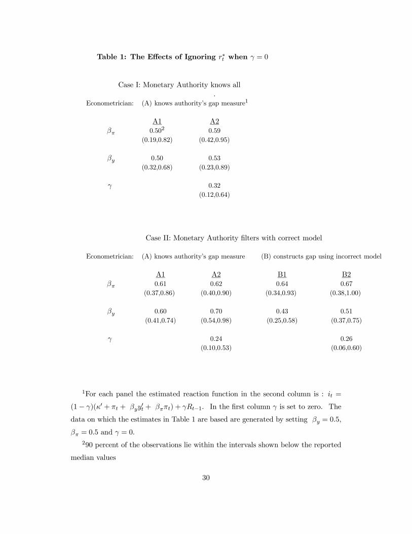
Table 1: The Effects of Ignoring r∗t when γ = 0

Case I: Monetary Authority knows all.

Econometrician: (A) knows authority’s gap measure1

A1 A2βπ 0.502 0.59

(0.19,0.82) (0.42,0.95)

βy 0.50 0.53(0.32,0.68) (0.23,0.89)

γ 0.32(0.12,0.64)

Case II: Monetary Authority filters with correct model

Econometrician: (A) knows authority’s gap measure (B) constructs gap using incorrect model

A1 A2 B1 B2βπ 0.61 0.62 0.64 0.67

(0.37,0.86) (0.40,0.90) (0.34,0.93) (0.38,1.00)

βy 0.60 0.70 0.43 0.51(0.41,0.74) (0.54,0.98) (0.25,0.58) (0.37,0.75)

γ 0.24 0.26(0.10,0.53) (0.06,0.60)

1For each panel the estimated reaction function in the second column is : it =

(1− γ)(κ0 + πt + βyy0t + βππt) + γRt−1. In the first column γ is set to zero. The

data on which the estimates in Table 1 are based are generated by setting βy = 0.5,

βπ = 0.5 and γ = 0.

290 percent of the observations lie within the intervals shown below the reported

median values

30

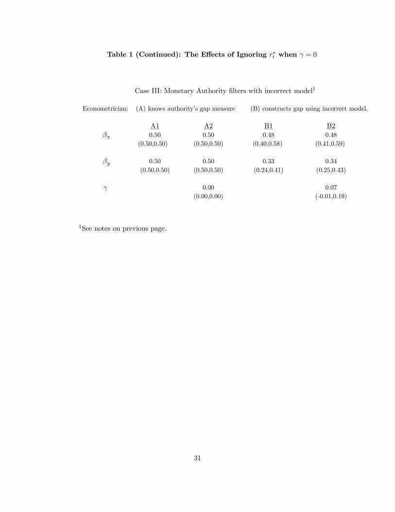
Table 1 (Continued): The Effects of Ignoring r∗t when γ = 0

Case III: Monetary Authority filters with incorrect model1

Econometrician: (A) knows authority’s gap measure (B) constructs gap using incorrect model.

A1 A2 B1 B2βπ 0.50 0.50 0.48 0.48

(0.50,0.50) (0.50,0.50) (0.40,0.58) (0.41,0.59)

βy 0.50 0.50 0.33 0.34(0.50,0.50) (0.50,0.50) (0.24,0.41) (0.25,0.43)

γ 0.00 0.07(0.00,0.00) (-0.01,0.19)

1See notes on previous page.

31

Table 2: The Effects of Ignoring r∗t when γ = 0.3

Case I: Monetary Authority knows all

Econometrician: (A) knows authority’s gap measure1

A12 A2βπ 0.48 0.54

(0.17,0.80) (0.26,0.91)

βy 0.42 0.63(0.25,0.59) (0.45,1.06)

γ 0.53(0.38,0.75)

Case II: Monetary Authority filters with correct model

Econometrician: (A) knows authority’s gap measure (B) constructs gap using incorrect model.

A1 A2 B1 B2βπ 0.58 0.62 0.62 0.68

(0.34,0.84) (0.41,0.92) (0.32,0.89) (0.40,1.03)

βy 0.47 0.74 0.35 0.53(0.28,0.62) (0.57,1.13) (0.16,0.50) (0.39,0.84)

γ 0.48 0.48(0.38,0.69) (0.33,0.71)

1For each panel the estimated reaction function in the first column is : it =

(1−γ)(κ0+πt+ βyy0t+ βππt)+γRt−1. In the second column γ is set to zero. The

data on which the estimates in Table 1 are based are generated by setting βy = 0.5,

βπ = 0.5 and γ = 0.3.

290 percent of the observations lie within the intervals shown below the reported

median values.

32

Table 2 (Continued): The Effects of Ignoring r∗t when γ = 0.3

Case III: Monetary Authority filters with incorrect model1

Econometrician: (A) knows authority’s gap measure (B) constructs gap incorrect model.

A1 A2 B1 B2βπ 0.47 0.50 0.46 0.48

(0.45,0.49) (0.50,0.50) (0.38,0.54) (0.41,0.59)

βy 0.39 0.50 0.26 0.34(0.36,0.42) (0.50,0.50) (0.18,0.34) (0.25,0.44)

γ 0.30 0.32(0.30,0.30) (0.27,0.41)

1See notes on previous page.

33

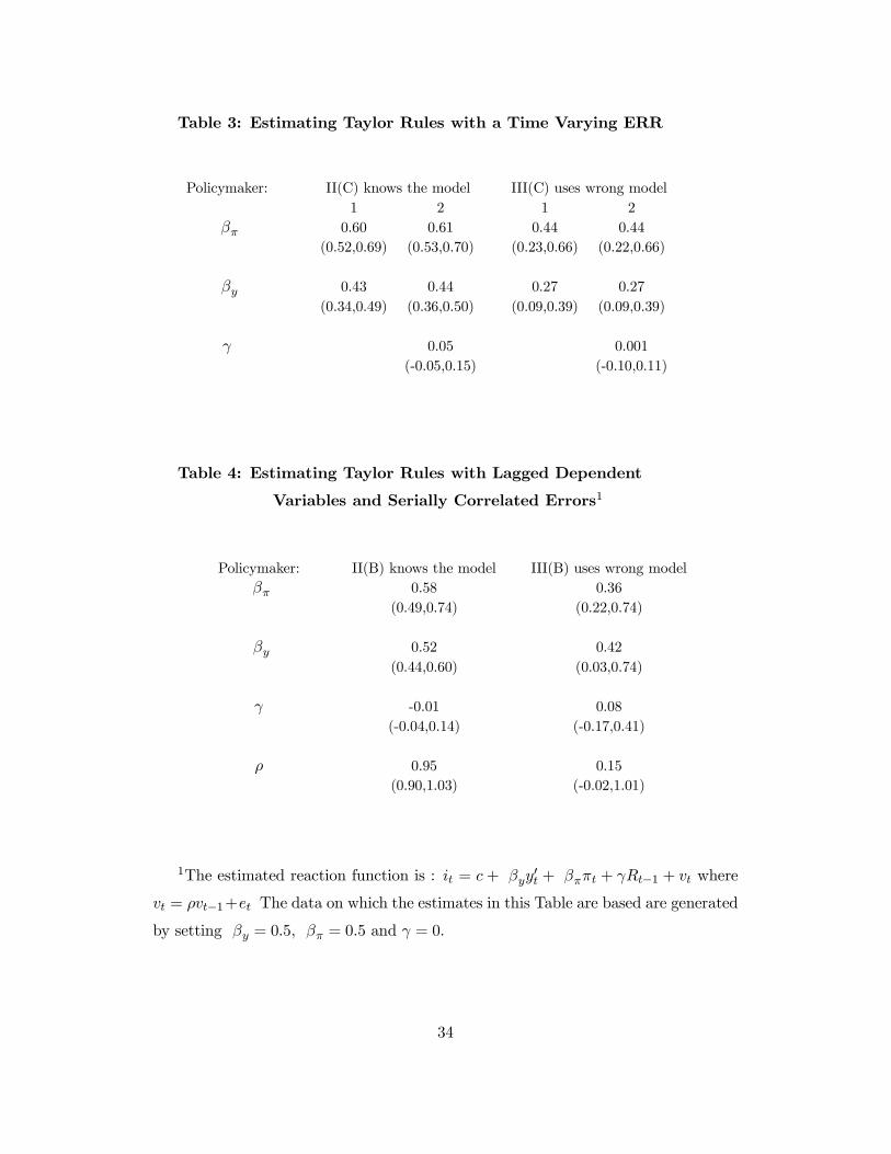
Table 3: Estimating Taylor Rules with a Time Varying ERR

Policymaker: II(C) knows the model III(C) uses wrong model1 2 1 2

βπ 0.60 0.61 0.44 0.44(0.52,0.69) (0.53,0.70) (0.23,0.66) (0.22,0.66)

βy 0.43 0.44 0.27 0.27(0.34,0.49) (0.36,0.50) (0.09,0.39) (0.09,0.39)

γ 0.05 0.001(-0.05,0.15) (-0.10,0.11)

Table 4: Estimating Taylor Rules with Lagged Dependent

Variables and Serially Correlated Errors1

Policymaker: II(B) knows the model III(B) uses wrong modelβπ 0.58 0.36

(0.49,0.74) (0.22,0.74)

βy 0.52 0.42(0.44,0.60) (0.03,0.74)

γ -0.01 0.08(-0.04,0.14) (-0.17,0.41)

ρ 0.95 0.15(0.90,1.03) (-0.02,1.01)

1The estimated reaction function is : it = c+ βyy0t + βππt + γRt−1 + vt where

vt = ρvt−1+et The data on which the estimates in this Table are based are generated

by setting βy = 0.5, βπ = 0.5 and γ = 0.

34

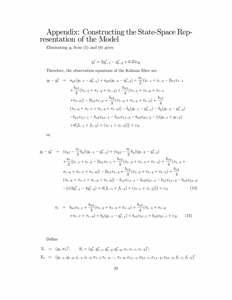
Appendix: Constructing the State-Space Rep-resentation of the Model

Eliminating gt from (5) and (6) gives

y∗t = 2y∗t−1 − y∗t−2 + 0.25ε4t

Therefore, the observation equations of the Kalman filter are

yt − y∗t = ay1(yt−1 − y∗t−1) + ay2(yt−2 − y∗t−2) +ar2{it−1 + it−2 − [bπ1πt−1

+bπ23(πt−2 + πt−3 + πt−4) +

bπ34(πt−5 + πt−6 + πt−7

+πt−8)]− [bπ1πt−2 + bπ23(πt−3 + πt−4 + πt−5) +

bπ34

(πt−6 + πt−7 + πt−8 + πt−9)]− by(yt−1 − y∗t−1)− by(yt−2 − y∗t−2)

−bx1x1,t−1 − bx2x2,t−1 − bx1x1,t−2 − bx2x2,t−2 − [c(gt−1 + gt−2)

+d(ft−1 + ft−2) + (zt−1 + zt−2)]}+ ε1t

or,

yt − y∗t = (ay1 − ar2by)(yt−1 − y∗t−1) + (ay2 −

ar2by)(yt−2 − y∗t−2)

+ar2{it−1 + it−2 − [bπ1πt−1 + bπ2

3(πt−2 + πt−3 + πt−4) +

bπ34(πt−5 +

πt−6 + πt−7 + πt−8)]− [bπ1πt−2 + bπ23(πt−3 + πt−4 + πt−5) +

bπ34

(πt−6 + πt−7 + πt−8 + πt−9)]− bx1x1,t−1 − bx2x2,t−1 − bx1x1,t−2 − bx2x2,t−2

−[c(4y∗t−1 − 4y∗t−3) + d(ft−1 + ft−2) + (zt−1 + zt−2)]}+ ε1t (14)

πt = bπ1πt−1 +bπ23(πt−2 + πt−3 + πt−4) +

bπ34(πt−5 + πt−6

+πt−7 + πt−8) + by(yt−1 − y∗t−1) + bx1x1t−1 + bx2x2t−1 + ε2t (15)

Define

Yt = (yt, πt)0, St = (y

∗t , y

∗t−1, y

∗t−2, y

∗t−3, zt, zt−1, zt−2)

0;

Xt = (yt−1, yt−2, it−1, it−2, πt−1,πt−2, ..., πt−9, x1,t−1, x2,t−1, x1,t−2, x2,t−2, ft−1, ft−2)0

35

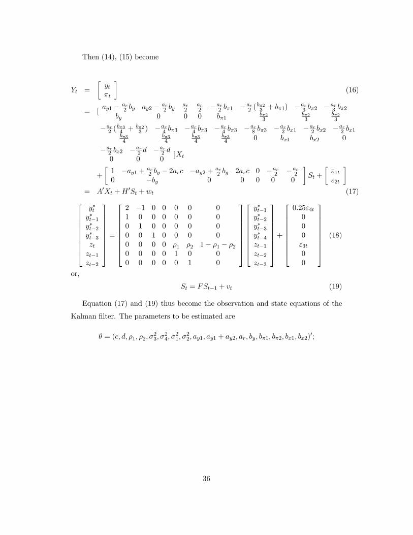
Then (14), (15) become

Yt =

·ytπt

¸(16)

= [ay1 − ar

2 by ay2 − ar2 by

ar2

ar2 −ar

2 bπ1 −ar2 (

bπ23 + bπ1) −ar

3 bπ2 −ar3 bπ2

by 0 0 0 bπ1bπ23

bπ23

bπ23

−ar2 (

bπ34 + bπ2

3 ) −ar4 bπ3 −ar

4 bπ3 −ar4 bπ3 −ar

8 bπ3 −ar2 bx1 −ar

2 bx2 −ar2 bx1

bπ34

bπ34

bπ34

bπ34 0 bx1 bx2 0

−ar2 bx2 −ar

2 d −ar2 d

0 0 0]Xt

+

·1 −ay1 + ar

2 by − 2arc −ay2 + ar2 by 2arc 0 −ar

2 −ar2

0 −by 0 0 0 0 0

¸St +

·ε1tε2t

¸= A0Xt +H 0St +wt (17)

y∗ty∗t−1y∗t−2y∗t−3ztzt−1zt−2

=

2 −1 0 0 0 0 01 0 0 0 0 0 00 1 0 0 0 0 00 0 1 0 0 0 00 0 0 0 ρ1 ρ2 1− ρ1 − ρ20 0 0 0 1 0 00 0 0 0 0 1 0

y∗t−1y∗t−2y∗t−3y∗t−4zt−1zt−2zt−3

+

0.25ε4t000ε3t00

(18)

or,

St = FSt−1 + vt (19)

Equation (17) and (19) thus become the observation and state equations of the

Kalman filter. The parameters to be estimated are

θ = (c, d, ρ1, ρ2, σ23, σ

24, σ

21, σ

22, ay1, ay1 + ay2, ar, by, bπ1, bπ2, bx1, bx2)

0;

36