time series analysis in road safety research using state space methods · · 2016-12-13time...
TRANSCRIPT

Time series analysis in road safetyresearch using state space methods
Frits Bijleveld
Time series analysis in road safety research using state space m
ethods Frits Bijleveld
ISB
N: 978-90-73946-04-0VU University Amsterdam
Time series analysis in road safety
research using state space methods
Frits Bijleveld

SWOV–Dissertatiereeks, Leidschendam, Nederland.
In deze reeks is eerder verschenen:
Jolieke Mesken (2006). Determinants and consequences of drivers emotions.
Ragnhild Davidse (2007). Assisting the older driver: Intersection design and in car
devices to improve the safety of the older driver.
Maura Houtenbos (2008). Expecting the unexpected. A study of interactive
driving behaviour at intersections.
Dit proefschrift is mede tot stand gekomen met steun van de Stichting
Wetenschappelijk Onderzoek Verkeersveiligheid SWOV.
Uitgever:
Stichting Wetenschappelijk Onderzoek Verkeersveiligheid SWOV
Postbus 1090
2262 AR Leidschendam
I: www.swov.nl
ISBN: 978-90-73946-04-0
c© 2008 Frits Bijleveld
Alle rechten zijn voorbehouden. Niets uit deze uitgave mag worden verveel-
voudigd, opgeslagen of openbaar gemaakt op welke wijze dan ook zonder
voorafgaande schriftelijke toestemming van de auteur.
VRIJE UNIVERSITEIT
Time series analysis in road safetyresearch using state space methods
ACADEMISCH PROEFSCHRIFT
ter verkrijging van de graad Doctor aan
de Vrije Universiteit Amsterdam,
op gezag van de rector magnificus
prof.dr. L.M. Bouter,
in het openbaar te verdedigen
ten overstaan van de promotiecommissie
van de faculteit der Economische Wetenschappen en Bedrijfskunde
op dinsdag 4 november 2008 om 15.45 uur
in de aula van de universiteit,
De Boelelaan 1105.
door
Frederik Deodaat Bijleveld
geboren te Voorburg

promotor: prof.dr. S.J. Koopman
copromotor: prof.dr.ir. C.A.G.M. van Montfort
Contents
1. Introduction 9
1.1. The main ideas of this research 9
1.2. Important issues in time series analysis of road safety data 12
1.2.1. Time dependence 12
1.2.2. Multiple road safety outcomes 16
1.2.3. Exposure data 17
1.2.4. Explanatory variables 19
1.2.5. Conclusions 23
1.3. Structure of this thesis 24
2. Safety, exposure and risk 28
2.1. Introduction 28
2.2. Risk exposure in road safety analysis 30
2.2.1. Statistical distributions 31
2.2.2. The distribution of accident counts 33
2.2.3. Over-dispersion 33
2.2.4. Gaussian approximations 34
2.2.5. The distribution of victim counts 34
2.2.6. The relation between trials and exposure 35
2.3. Traffic volume and accident occurrence 36
2.3.1. The relation between ‘traffic volume’ and the number of
accidents 36
2.3.2. A remark on traffic volume and multiparty accident oc-
currence 38
2.4. Summary and discussion 38
3. Multivariate structural time series models 41
3.1. Introduction 41
3.2. The concept of state and its observation 42
3.3. The latent risk time series model 45
3.3.1. A basic latent risk observation model 45
3.3.2. The role of the dynamic relation among states 47
3.3.3. Specification by means of linear structural models 54
3.3.4. Linear measurement equations 60
3.3.5. General state space model specification 62
3.3.6. Estimation of parameters and latent factors, missing data 62
3.3.7. Kalman smoother, auxiliary residuals 64
3.3.8. Diagnostic checking 64
3.4. Applications 65
3.4.1. State space DRAG-similar models 65
3.4.2. Estimating the registration level of accidents involving
hospitalised victims 71
3.5. Non linear extensions 77
3.5.1. Introduction 77
3.5.2. Mixing additive and multiplicative models 78
3.5.3. Further generalisations 79
4. The covariance between the number of accidents and victims 80
4.1. Introduction 80
4.1.1. The need for multivariate modelling of influences on road
safety 80
4.1.2. The issue of dependence among outcomes 81
4.1.3. An approximating solution 82
4.1.4. Overview of the paper 84
4.2. The covariance structure of road safety related
outcomes 85
4.2.1. Introduction 85
4.2.2. Results 85
4.3. Simulation studies 86
4.4. Examples 89
4.4.1. The mortality ratio 89
4.4.2. Multivariate state space modelling and the Kalman filter 91
4.4.3. The relative error of the variance estimate of the loga-
rithm of a Poisson distributed random variable 91
4.5. Conclusions 92
5. Model-based measurement of latent risk in time series 94
5.1. Introduction 94
5.2. The statistical framework 96
5.3. Case I: a two-dimensional insurance LRT model 100
5.4. Case II: a three-dimensional credit card LRT model 103
5.5. Case III: a multiple exposure LRT model 106
5.6. Conclusions 108
6. Multivariate nonlinear time series modelling of exposure and risk in
road safety research 109
6.1. Introduction 109
6.2. Data description 112
6.3. The multivariate nonlinear time series model 113
6.3.1. Specification of model and assumptions 113

6.3.2. Unobserved stochastic local linear trend factors 115
6.3.3. Observation equation 115
6.3.4. Nonlinear state space model formulation 116
6.4. Estimation of parameters and latent factors 118
6.5. Empirical results: estimation and model selection 121
6.5.1. Parameter estimation results 122
6.5.2. Signal extraction: trends for exposure and risk 123
6.5.3. Model fit 124
6.5.4. External validation 126
6.6. Implications for road safety research 127
6.7. Conclusions 128
7. The likelihood filter: estimation and testing 130
7.1. Introduction 130
7.2. Maximum likelihood approach to filtering 132
7.2.1. Gaussian maximum likelihood approach to filtering 132
7.2.2. General maximum likelihood approach to filtering 132
7.3. Laplace approximation of the likelihood 133
7.4. Simulation studies 134
7.5. Applications 141
7.5.1. Volatility: pound/dollar daily exchange rates 141
7.5.2. The effects of precipitation on road safety 142
7.5.3. Conclusions 155
7.6. Discussion and conclusions 155
8. Conclusions 157
References 163
Author index 173
Appendix A. 177
Appendix B. 187
Appendix C. 194
Samenvatting 199
Dankwoord 207

1. Introduction
1.1. A short description of the main ideas of this research
In this thesis we present a comprehensive study into novel time series models
for aggregated road safety data. The models are mainly intended for analysis
of indicators relevant to road safety, with a particular focus on how to measure
these factors. Such developments may need to be related to or explained by
external influences. It is also possible to make forecasts using the models. Rel-
evant indicators include the number of persons killed per month or year. These
statistics are closely watched by government agencies and the public, and their
relevance to society is not disputed. A large body of research is devoted to the
improvement of road safety. To that end, changes in the number of accidents
or victims are often attempted to be explained by (changes in) factors such as
exposure, policy, driving under the influence of alcohol, speeding by drivers.
Some factors such as policy changes can be directly observed (although com-
pliance with policy and law may not). Other factors can be observed in theory
but in practice their measurement is either difficult or very expensive. Exam-
ples of such factors are exposure, which is measured using surveys and vehicle
counting systems, and percentage of drivers exceeding the legal blood alcohol
concentration limit, which is measured using road side surveys. Finally, some
factors are even harder to observe such as driver skill or experience.
The methodology used by the novel approach introduced in this thesis is de-
signed to address potential inaccuracies of data, both in dependent variables
and in explanatory variables. The methodology also addresses the potential
multivariate nature of road safety analysis problems due to multiple depen-
dent road safety outcomes like the number of accidents and victims. The first
aspect results in non-homogeneous observation error variances and the needs
for a multivariate approach to modelling. The second aspect introduces struc-
tural but time varying covariance among (multivariate) observation errors.
Both issues are accounted for by readily available statistical techniques derived
from the Kalman filter (Kalman, 1960). In this thesis a special form of Kalman
(1960)’s model which is referred to as a structural time series model is further
developed. Structural time series models originate from Muth (1960), and were
made popular by Harvey (1983), and applied in multivariate form by Harvey
and Koopman (1997). A special form of the latter model designed for road
safety risk analysis is developed in this thesis and was published as Bijleveld,
Commandeur, Gould, and Koopman (2008). This model is combined with an
9

approach to estimating the structural covariance among accident related data
in Chapter 4, which was published in Bijleveld (2005).
Structural time series models were first applied in road safety analysis by Har-
vey and Durbin (1986). In Harvey and Durbin (1986) the consequences of the
introduction of the seat belt law in the United Kingdom in 1983 is evaluated.
The same methodology was later applied to a seat belt use change in West-
Germany by Ernst and Bruning (1990) and to a re-analysis of the introduction
of the seat belt law in the Netherlands by Bos and Bijleveld (1991). Other ap-
plications in road safety analysis based on this method are by Lassarre (2001),
Scuffham and Langley (2002), and COST329 (2004), and in recent PhD theses
the method is applied by Scuffham (1998), Christens (2003), Gould (2005) and
Van den Bossche (2006).
Given the fact that time series are analysed, the choice for structural time series
models was mainly made because the time series can then be decomposed into
interpretable components. This allows for the interpretation of risk and other
developments while such developments are not directly observed.
In addition, estimating interpretable components also allows for limited vali-
dation of their development, as the interpretable parts should at least have a
reasonably plausible developments. In case additional information is available
pertaining to the development of interpretable components, such information
can be included in the model. Adding such additional information allows the
researcher to use as much available information as possible. The possibility
of a limited form of validation of the results is a substantial advantage of the
structural time series approach over more black-box like analysis alternatives.
One of such alternatives are ARIMA models as applied in Box and Tiao (1975),
see also Box and Jenkins (1976) and many textbooks.
The structural approach presented in this thesis allows the researcher to distin-
guish factors that affect road safety from factors that affect the way road safety
is observed. A change in a travel survey is not likely to change travel patterns,
it is more likely to change travel data. Furthermore, it is also possible to specify
on which component (or components) a particular factor should have an effect
according to theory or hypothesis, which can then be further verified.
As a side effect, the multivariate approach introduced in this thesis in which
traditional dependent variables as well as variables traditionally treated as ex-
planatory variables are simultaneously treated as dependent variables has an
additional benefit. A regression coefficient associated with the relation be-
10
tween an explanatory variable and a dependent variable can be absorbed in
the model.
The special case where exposure is the explanatory variable is given promi-
nent attention in this thesis. In the log linear context, as used in Chapter 3
and Chapter 5, a regression coefficient as described in the handbook by Elvik
and Vaa (2004, p. 49) and many other studies, is absorbed in the model. Elvik
and Vaa (2004)’s approach has the advantage of (approximately) accounting
for a non linear relation between traffic volume and the number of accidents,
as suggested by for instance Hauer (1995). However, Elvik and Vaa (2004)’s
approach has the disadvantage of limiting the comparability of its results be-
tween models that have different coefficients. The model developed in Chap-
ter 3 and Chapter 5 estimates development for risk as the ratio of the number
of accidents per vehicle kilometre, which should be comparable between mod-
els. Other models, described in Chapter 3 are inspired by and share properties
of the DRAG (demande routiere, accidents et leur gravite) framework by Gaudry
(1984) and Gaudry and Lassarre (2000).
The first study within the context of this thesis was Bijleveld (1999). The objec-
tive of Bijleveld (1999) was to improve the reliability of short-term prognosis
of general road safety outcomes, to be used as part of an annual review of the
development of road safety in the Netherlands. Specifically, such prognoses
were intended to be used to determine whether or not road safety outcomes in
the reviewed year were in line with what could be expected from road safety
developments just before that year. A comprehensive analysis of changes in
the development of road safety related indicators could help the road safety
researcher detect recent general changes in road safety conditions, if any. After
Bijleveld (1999), the objective was extended to the analysis of the development
of aspects of road safety in general, resulting in this thesis.
A primitive form of the model was developed during work on the COST329
(2004) report in the second half the 1990’s. The simplicity of the implemen-
tation of the EM algorithm (Expectation Maximisation, e.g. Dempster, Liard,
and Rubin, 1977; McLachlan and Krishnan, 1997) for state space estimation
found in Fahrmeir and Tutz (1994) and others, which easily allowed for a gen-
eral multivariate implementation of the approach taken by Harvey and Durbin
(1986), was also of importance. The final publication of COST329 (2004) was
delayed, and as a result the approach was first published in Bijleveld (1999).
The results presented in this thesis are aimed at providing better and statis-
tically more reliable options for time series analysis of road safety data. The
11
analyses performed in this thesis are not intended to answer specific road
safety questions, but are intended to illustrate the application of the methods
introduced in this thesis.
1.2. Important issues in time series analysis of road safety
data
In this section four central issues involved in time series analysis of road safety
data are presented: time dependence, multiple road safety outcomes, exposure
data, and other explanatory variables.
1.2.1. Time dependence
When a specific condition in road traffic suddenly changes at a certain time
point, it is often to be determined whether (or not) a relevant road safety indi-
cator changed at about the same time point. The opposite also occurs: when
a specific road safety indicator changed at a certain time point, it is often to
be determined whether (or not) a relevant road traffic condition changed at
about the same time point. A classical approach to statistical analysis in this
situation would be to select a type of accident that should be affected by the
change (which is called the experimental group), and a type of accident that
should not be affected by the change (which is called the control group). Then
both accident counts for a period before and after the change are compared in
a 2×2 table:
Count before after
experimental group eb ea
control group cb ca
In a typical before/after study, the rate before eb/cb and after ea/ca are com-
pared. It has to be assumed that the rates would remain constant if the condi-
tion in road traffic had not changed. If the rate e/c was constantly decreasing,
eb/cb would be larger than ea/ca, if only for that reason. This drop could be
falsely attributed to the sudden change in road traffic conditions. There are
numerous reasons why the rate could change with time. For instance, when
the experimental group is moped victims, and the control group is bicycle vic-
tims, the rate will change when bicycles are getting preferred over mopeds for
travel. Therefore it is wise to determine the rate e/c for a number of periods in
the before and after period. Then verify that the rate e/c is reasonably constant
12

in the before and after period, before a change in this rate can be attributed to
the change in road traffic conditions. If this analysis is performed, and a se-
ries of rates e/c is available for a period of time, it is also wise to determine
whether the drop in the rate occurred about the time of the change in road
traffic conditions or not. If this is not the case, some other influence may have
caused the drop (this possibility can never be excluded). Furthermore it can
be determined whether or not the change in the rate is exceptional. If similar
drops in the rate occur regularly and cannot be explained, there is no reason to
assume that this particular drop is not coincidental but caused by the change
in road traffic conditions, while others are considered coincidental.
The analysis steps described above, are regularly performed in time series
analysis. In the first step, a trend is determined, in the second and third step
a so-called structural break is identified (both its location (where and when it
occurred) and whether it is significant).
For this reason alone it can be suggested to perform a more elaborate time
series analysis than a before/after study, which itself is a rudimentary analysis
of time ordered data, with just two time points. More reasons can be suggested
to make this choice.
When a specific condition in road traffic does not change suddenly but changes
gradually it is not trivial to use a before/after study. In such situations (time
series) regression analysis is currently most often applied.
There are other ways in which time dependence may affect the analysis of road
safety data. For example, time dependence implies some structure among ob-
servations. There is sufficient reason to at least consider time dependence in
road safety analysis. If data collected over a longer period of time are con-
sidered, the general road safety situation is likely to have changed as, among
other conditions, road and vehicle design may have improved. If this is the
case, observations close in time will resemble each other more than observa-
tions further apart in time. This phenomenon is reflected in the development
of many road safety related features like the number of fatally injured victims
in road accidents in Figure 1.1. The road safety situation in 1970 will say lit-
tle about the road safety situation in 2000, while the road safety situation in
2007 may give a rather accurate idea of what the road safety situation in 2008
probably will be.
13

1950 1960 1970 1980 1990 20001000
1500
2000
2500
3000
Figure 1.1. The development of the numberof police recorded fatally injured victims inroad accidents (1950–2000) in the Netherlands.Source: CBS (2000).
Most statistical models require that the difference between the model and data
is purely coincidental and no two differences are related1. Technically this
means that the so-called disturbances (the difference between the observed
and the prediction by the true model, which is not observed) are required to be
independent of each other. Failure to satisfy this requirement may lead to over
or under estimation of model uncertainty, which again may lead to statistical
tests being too conservative or worse, not being conservative enough. This
in turn may lead to falsely positive identification of relationships or interven-
tions in road safety analysis. See, for instance Scheffe (1967, Chapter 10) for a
discussion on violations of assumptions on the disturbances in a linear model,
which also includes uniformity of the variance of the disturbances. This poten-
tial problem cannot be ignored, and accounting for it is the second way time
dependence affects the analysis of road safety data.
Model residuals are differences between observed values and the predicted
values from the estimated model, as depicted at time point “4” on the left
hand side of Figure 1.2. Model residuals are observed in contrast to the distur-
bances. The residuals in this figure are positive for the first two time points, the
next residual is approximately zero, then three residuals are negative, the next
three residuals are positive, the following three residuals are again negative,
etc. Most models require that disturbances are independent of one another,
which roughly speaking means that knowing one residual (which estimates a
disturbance) should not help in predicting the next. In the example shown in
Figure 1.2 the requirement of independence of the disturbances is most likely
violated.
1Models exist which require an independent source of error, not necessarily describing thedifference between the model and data.
14

0 5 10 15 20
16
17
18
19
20
Figure 1.2. Theoretical development of the number of accidents (hy-pothetical development is 20 − t/5 + sin (t) for t = 1, . . . , 20) anda linear regression over the first 16 observations (to the left of thevertical reference line) plus a forecast (to the right of the verticalreference line). The differences between the dots and the (straight)line (to the left of the vertical reference line) are called the modelresiduals. The differences to the right of the vertical reference lineare technically not model residuals, as they were not included in theregression. It can be seen that consecutive residuals tend to sharethe same sign.
An example of the first way in which time dependence may affect the analy-
sis of road safety data is correcting for time dependencies in model residuals
for (short-term) prognosis. This can be understood from the example devel-
opment presented in Figure 1.2. It is not uncommon to have a development
of the number of accidents similar to Figure 1.2, where there is a linear trend
(in this case fixed at 20 − t/5) and some fluctuation around it, (for example
sin (t)), yielding the function 20 − t/5 + sin (t) for t = 1, . . . , 20. From Fig-
ure 1.2 it is clear that the forecast for t = 17, . . . , 20 obtained by extending
the linear regression line (as depicted by the straight line in Figure 1.2) can be
substantially improved by using the knowledge that the observations follow a
pattern of being positioned over and under the regression line. Roughly, this is
what considering ‘time dependence’ of model residuals amounts to: account-
ing for an empirically revealed structure in residuals. In general, the dynamic
structure is unknown, and much like in this example it is attempted to build a
description of the dynamic structure. First a linear trend (or another structure
suggested by theory) is fitted. Then the residuals are studied. If those residu-
als do not reveal a structure, the model may be adequate. If not, the dynamic
structure is adapted. There are a number of approaches to adapt the dynamic
structure, one of them is chosen later in this thesis.
15

1.2.2. Multiple road safety outcomes
One important aspect of road safety (time series) analysis is that road safety
cannot be measured unambiguously. There is no unique measure of road
safety. Usually, road safety is measured in terms of the amount of ‘lack of road
safety’, for instance the number of accidents occurring per time unit. Even if
the number of accidents is selected as the measure of road safety, it could still
be all accidents, injury accidents, serious accidents or fatal accidents, or other
types of accidents. But even then the number of victims per accident may be
of interest, as well as the number of fatalities per accident.
It should further be considered that influences on road safety may primarily
affect certain parts of the road safety process. For instance, it is sometimes
claimed (and disputed) that the use of seat belts primarily has an effect on ac-
cident consequences, not on accident occurrence. If it is true that the use of seat
belts primarily has an effect on accident consequences, it would be sufficient
to study the number of victims. Risk adaptation theories (such as for exam-
ple Wilde (1994) and Summala and Naataanen (1988)) state that developments
that could be expected from theory may be counteracted due to behavioural
adaptation, in this case possibly increased speeding by drivers. If this is true,
not only the accident consequences in terms of the number of injuries need to
be considered, but also the number of accidents. Even if the original theory is
assumed to be true, it is sensible to study both the development of the number
of accidents and the number of victims.
Assume a study into the effect of the introduction of a seat belt law on road
safety is to be conducted. It is possible that in the period in which the seat
belt law was introduced, other influences had an effect on road safety. Such
influences may have had an effect on the indicators that are considered to be
relevant to the safety effect of seat belts. If the effect of the seat belt law is to be
determined, one may need to correct for other influences. Therefore the mod-
elling approach should be able to disentangle multiple effects. These effects
may have had an impact on the number of accidents or victims of a certain
type, or both, which is best done by modelling them simultaneously. How-
ever, the number of accidents and the number of victims resulting from these
accidents are correlated, and this correlation should be accounted for in the
analysis. In summary, the modelling approach should be capable of simulta-
neously treating at least two dependent variables (in case of the example above
these would be the number of accidents and victims), and their covariance.
16

Another reason to consider multiple road safety outcomes is that although
road safety interventions may be introduced to reduce certain accident out-
comes, they may also – hopefully to a lesser extent – increase certain other
accident outcomes. In general, the accumulated effect of road safety interven-
tions is considered most important as it indicates the net effect to society. In
specific applications the differentiated effect of road safety interventions needs
to be studied, for instance to test hypotheses on theories.
1.2.3. Exposure data
In France more accidents occur in road traffic than in the Netherlands, but
does that necessarily mean that road traffic is safer in the Netherlands than in
France? Is it not the case that France is a much larger country than the Neth-
erlands, and thus has more potential to have accidents in road traffic than the
Netherlands? One would expect an imaginary country twice the Netherlands
in every respect and otherwise completely equal to have twice as many acci-
dents as the Netherlands. This reasoning is often used to justify using accident
rates in terms of the number of accidents per unit of scale when comparing dif-
ferent entities such as road sections or countries. In this example, the number
of accidents for the imaginary country would be divided by two as the coun-
try potentially has twice as many accidents. The potential to have accidents
(or victims) is generally referred to as exposure in road safety analysis.
Accounting for differences in exposure is not always straightforward. For in-
stance, when comparing the number of fatal accidents in France to the Neth-
erlands (which is about 6.5 to 1), the difference in country size (about 552.000
km2 for France and about 42.000 km2 for the Netherlands, including water sur-
face) could be used to account for differences between France and the Nether-
lands. This would make the Netherlands in this respect less safe than France.
Such a figure would ignore differences in land use (notably population den-
sity), which could be considered a disadvantage. Alternatively, population
size could be used, which was about 61 million for France and about 16 mil-
lion for the Netherlands in 2007. Using population figures as a measure of
exposure would present France as less safe than the Netherlands. A drawback
of using population figures may be that such figures may not sufficiently ac-
count for differences in road use: in a large country like France, the population
may have to travel longer distances. In order to improve on such figures, traf-
fic volume (the number of kilometres or miles driven on the road by vehicles)
or travel volume (the number kilometres or miles travelled on the road by per-
sons) are often used when available. Such figures may better represent the
exposure of a country than its size or number of inhabitants.
17

It should be noted that, although traffic volume is mostly preferred as a mea-
sure of exposure, it is the research question that determines the optimal expo-
sure measure. In practice the researcher not just selects one available exposure
measure, rather, exposure measures are selected for a specific purpose. The
number of fatalities per unit of population per year is sometimes used specifi-
cally to be compared with other mortality rates. For similar reasons, the number
of victims per unit of population per year can be used to compare with other
incidence rates. When road accidents are compared with work accidents, then
the time spent in travel is probably the preferred choice.
It should further be noted that, no matter how accurate traffic or travel volume
appears to be measured, such measurements cannot be considered an exact es-
timate of exposure. As some information on traffic or travel volume is obtained
through travel surveys, these data are by nature subject to random error. An-
other reason is that it is not only the amount of travel that is important to road
safety, but also the conditions under which the travel took place.
As an example of the uncertainties concerning traffic volume data, consider
the Dutch travel data using mopeds presented in Figure 1.3. In the left hand
panel of this figure the number of person kilometres2 is presented for mopeds,
together with the number of police registered accidents with killed or hospi-
talised victims between mopeds and cars. The grey area depicts the point wise
95% percent confidence intervals for the person kilometres. These intervals are
based on an estimate of the error due to sampling only – an estimate of the error
due to respondents providing erroneous data is not available – therefore the
actual error is likely to be larger. In the right hand panel of Figure 1.3 the rel-
ative error based on Slootbeek (1993) and CBS (2003) (right hand panel, solid
line, left hand axis) is presented together with a plot of 1/√
number of trips
(dashed line). This plot reveals that the relative sampling error for the to-
tal moped travel in 2005 is about 16% (left hand scale). The relative error of
moped travel for separate age groups will be substantially larger. In 1994 and
1995 the survey was substantially extended. In 1999/2000, the survey struc-
ture has changed. Over the last few years the survey size has been reduced
while the use of mopeds has also decreased. This resulted in the relative accu-
racy of moped data being at about the same level as it was near the end of the
1980’s.
2Driver kilometre data are not available, but the development of driver kilometres shouldbe similar to the development of passenger kilometres. Moped occupancy appears to be rela-tively constant based on a moped helmet survey (Ermens and van Vliet, 2006) for 2002–2005,where it was found that on about 11% of the mopeds evaluated a passenger was present.
18

0.6
0.8
1.0
1.2
1.4
1.6
1985 1990 1995 2000 2005
800
1000
1200
1400
1600
0.015
0.020
0.025
0.030
0.035
1985 1990 1995 2000 2005
0.08
0.10
0.12
0.14
0.16
0.18
Figure 1.3. Traffic volume and accident data for mopeds in the Netherlands 1985–2006. Left handpanel, left hand axis, dots: the number of police registered accidents with killed or hospitalisedvictims between mopeds and cars. Left hand panel, right hand axis, solid line: the number ofperson kilometres (billion) using mopeds in the Netherlands. The grey area depicts the pointwise 95% percent sampling confidence intervals for the person kilometres based on Slootbeek(1993). Right hand panel, left hand axis, solid line: relative sampling error in person kilometresbased on Slootbeek (1993). Right axis, dashed line: 1/
√
number of trips.
In the left hand panel of Figure 1.3, the traffic volume appears to go up and
down by a substantial amount near the end of the 1980’s, while the accident
counts seem relatively stable. Ignoring the fact that the traffic volume data
in this case are not accurate, one may conclude that both the traffic volume
and the risk (being the ratio of the number of accidents to the traffic volume)
fluctuated substantially in this period, which was probably not the case.
The topic of exposure is further discussed in Chapter 2, which also discusses
whether exposure affects road safety linearly or non linearly, as for instance
argued by Hauer (1995).
1.2.4. Explanatory variables
Besides exposure, the development of road safety can be influenced by devel-
opments in many areas such as road design, vehicle technology, education, de-
mography, weather, economy, etc. Quantitative information on such develop-
ments is regularly obtained from separate research results. The studies which
provide such results can be regularly and consistently conducted surveys, as
is the case with the travel survey in the Netherlands, or population figures ob-
tained from censuses or registers. However, studies may come from different
disciplines, may have different viewpoints, and are often limited by design to
some subsection of the complete road safety field. As road safety time series
analysis typically considers a longer period of time, it is likely that study de-
sign and purpose have changed over time, although such studies generally
19

still measure the same phenomenon. It is possible that such changes could
influence analysis results, the impact of which should be minimised.
Example: drink driving data
One example of a case where data collection may potentially affect analysis
results is data on the percentage of drivers exceeding the legal blood alcohol
concentration limit (drink driving). It is commonly assumed that drink driv-
ing is a risk increasing factor. When the consequences of drink driving for road
safety are to be determined, it is important to know how many drivers are ac-
tually exceeding the legal blood alcohol concentration limit. In Figure 1.4 the
percentage of car drivers tested to have a Blood Alcohol Concentration (BAC)
larger than 0.5 g/l (0.5 grammes per litre) in the Netherlands is given. The re-
sults are obtained from a number of surveys intermittently conducted during
autumn weekend nights, starting in 1970. This example demonstrates another
case of an important explanatory variable that in general should measure the
same phenomenon (the percentage of drivers exceeding the legal blood alcohol
concentration limit). Due to changes in measurement and scale of the survey,
the series of data is not fully consistent and not systematic in its accuracy. Fur-
thermore, the measurement for one year is distorted, possibly as a result of
the fact that the focus of the survey that year was directed at the introduction
of a new drinking driving law. Finally, the studies are justifiably focused on
assessing the worst extent of the problem by measuring drink driving in a pe-
riod, weekend nights, where the percentage of drivers under the influence of
alcohol is expected to be largest. The measure is therefore unlikely to represent
drink driving in general road traffic.
On the first of November 1974 a new law introducing the 0.5 g/l BAC legal
limit became effective in the Netherlands. At the same time, chemical test
tubes for road side testing were introduced. This time point is marked by
the first vertical reference line in Figure 1.4. SWOV (1978) reports that the
measurement for that year (1.5 %) was based on the average of observations
specifically taken one weekend immediately before the introduction of the law
(the weekend of 25–27 October 1974, 12% violations) and two larger surveys in
weekends immediately after the introduction of the law (the weekends of 8–10
November and 22–24 November 1974, 1% violating the law). Given the ob-
servation in 1975 and the fact that 12% violations were recorded the weekend
before the introduction of the law (and 15% in 1973), it may not be realistic to
consider the observation of about 1.5% for 1974 as being representative for the
percentage of drivers exceeding the 0.5 g/l BAC limit in the whole of 1974.
20

1970 1975 1980 1985 1990 1995 2000 2005
0
2.5
5
7.5
10
12.5
15
Figure 1.4. Percentages of car drivers having a Blood Alcohol Con-centration (BAC) exceeding 0.5 g/l in the Netherlands based on sur-veys taken in the autumn during weekend nights (see, Mathijssen,2004). The survey was not conducted every year. Dots mark avail-able data points.
In 1984 (marked by the second vertical reference line in Figure 1.4) electronic
alcohol breath test devices for selection purposes were introduced (blood tests
were still needed for legal confirmation). Starting in 1985 a gradual change
from selective to random police alcohol controls took place, which changed the
population sampled. As of the first of January 1987 (marked by the third ver-
tical reference line), results of alcohol breath tests could be used for evidential
purposes (in addition to blood sample tests). As of the first of November 1992,
heavier fines for drink-driving were introduced. The survey initially consisted
of about 3,000 observations, by the early 1990s this number increased to about
15,000, and at the end of the series there are about 30,000 observations. More-
over, the survey has not been conducted each year. Missing data are interpo-
lated in Figure 1.4. However, the percentages not necessarily dropped linearly
starting in 1984, the first of three years in which no surveys were conducted
(as is noted by Mathijssen (2004)). If accident occurrence is indeed related to
alcohol use by drivers, a drop in alcohol use by drivers could be reflected by a
drop in accident occurrence. A drop in accident occurrence at a later year may
indicate that alcohol use could have dropped later, but may not be conclusive.
An estimate of the missing values based on the accident development is likely
more reliable than the linear interpolation.
The example concerning drink-driving data as well as the discussion on expo-
sure data suggest that explanatory variables should not be considered at face
value. Each explanatory variable should be carefully considered and weighed.
21

In both examples the survey size varies over time, effectively meaning that
the accuracy of the data is not the same for all time points. As a result, het-
eroscedasticity among observation errors should be considered.
Further issues
Apart from the reliability of an explanatory variable, another important issue
to consider is its validity, that is, whether or not it actually represents what it
is supposed to represent. For instance, in the drink driving example, the data
actually refer to autumn weekend nights, not full days. This means that the
scope of the data should be considered. In road safety research one quite often
is forced either not to use an explanatory variable or to assume that the ‘true’
explanatory variable (in this case drink driving on average days) has a ‘similar’
development to the one actually available, or to try and find confirmation of
this assumption from other studies. Exposure data are subject to similar prob-
lems. The exposure data are obtained from household surveys CBS (2003) and
AVV (2005). As the sampling unit is households3, the persons in the survey
are almost exclusively residents of the Netherlands (but not necessarily Dutch
nationals). This implies that travel data for non-residents of the Netherlands is
not included in the survey, thus the survey does not represent all travel in the
Netherlands.
The scale of studies providing explanatory variables may vary between the mi-
croscopic level – at the level of individual accidents – and the (supra) national
macroscopic level of aggregated data. Generalisations of many such ‘pieces’
of information may be necessary to complete the ‘puzzle’ of road safety. A
microscopic level study may reveal the effect of seat belts on victims, while
macroscopic level studies may establish the effect a law on seat belt use has on
society.
As the type of analysis targeted in this research tends towards macroscopic
(aggregated) level analysis rather than microscopic level analysis, consequen-
ces of using results from lesser aggregated studies should be considered. For
instance, while a microscopic level study into the influence of weather on road
safety may reveal that the average temperature explains some variation in acci-
dent counts, the average temperature over a year may not. As a second exam-
ple, Eisenberg (2004, p. 637) finds that “in a typical state-month pair in the US
from 1975 to 2000, increased precipitation is associated with reduced fatal road
traffic crashes. More precisely, an additional 10 cm of rain in a state-month is
associated with a 3.7% decrease in the fatal crash rate”. Later he states: “First,
when the regression analysis is conducted with the state-day, rather than the
3Actually addresses are sampled. Some addresses may have more households.
22

state-month, as the unit of observation, the association between precipitation
and fatal crashes is estimated to be positive and significant, as in the literature.”
(Eisenberg, 2004, p. 637). Eisenberg (2004) continues to explain the importance
of lagged precipitation data in his (daily) model, effectively introducing a time
series model. This shows that different aggregation levels may yield opposite
results.
1.2.5. Conclusions
In this chapter it is demonstrated that travel volume data and data on the per-
centage of drivers exceeding the legal blood alcohol concentration limit (both
derived from surveys) have to be considered as observed under error. How-
ever, it is not just travel or alcohol surveys that are observed under error. Sim-
ilar arguments would hold for data derived from surveys like crash helmet
use on mopeds (Ermens and van Vliet, 2006), and many others. If a variable
is measured under error this means that instead of the true value, by coinci-
dence a different value is used, which can be considered random fluctuation
from the true value. In case of traffic volume data, the true value would be
the number of kilometres driven, while the value actually used would be the
number of kilometres driven based on the randomly selected respondents of
a survey, instead of the entire population. In general, the fluctuations are on
average (expected to be) nil. However, its variance, which is a measure of the
statistical accuracy of the data is larger than nil.
The issue of the potential random fluctuations in exposure and other explana-
tory data is mostly ignored in road safety analysis, probably as often no infor-
mation with respect to the statistical accuracy of the data is available. In many
cases, however, the consequences of ignoring statistical inaccuracy of expo-
sure or explanatory data may be negligible compared to other inaccuracies.
Neglecting the statistical accuracy of the data is not always warranted. For
instance disaggregate traffic volume data (traffic volume data for subgroups)
may be subject to substantially larger sampling errors than aggregate data (as
described in the example on moped travel), up to more than 100% sampling
error. Furthermore, there is no reason not to account for the inaccuracy of the
data when it is possible to do so.
Therefore it is important to consider the possibility of random fluctuations
in the explanatory data as well as random fluctuations in the accident data.
Considering possible random error in explanatory variables as well as in de-
pendent variables implies an ‘errors-in-variables’ approach (see, Seber and
Wild, 1988, Chapter 10). This approach essentially treats explanatory varia-
bles (which are assumed to have error) as dependent variables alongside the
23

original dependent variables. As a result, models are multivariate in the sense
of multiple dependent variables. Besides the ‘errors-in-variables’ argument,
there are further reasons to consider road safety analysis problems multivar-
iate. It is argued that road safety cannot be measured unambiguously as no
unique measure of road safety is available. Depending on the research ques-
tion road safety can be measured in terms of the number of accidents or vic-
tims, and combinations of these.
In this thesis road safety is therefore considered inherently a multivariate prob-
lem, that should preferably be analysed accordingly. Furthermore, the conse-
quences of time dependence should be considered, not only in view of reli-
ability of statistical tests, but also in view of making forecasts of future road
safety indicators. It will be demonstrated in Chapter 3 that considering time
dependence allows for an intuitive treatment of missing data as well.
A sufficiently flexible general framework to statistical time series analysis is
already available, based on (derivations of) the Kalman filter (Kalman, 1960).
This framework also handles non-homogeneous observation error variances
in a straightforward manner. In this thesis a special form of (Kalman, 1960)’s
model called a structural time series model is further developed in a multivar-
iate dimension, specifically designed for road safety risk analysis.
Given the fact that time series are analysed, the choice for structural time series
models was mainly made because the time series can then be decomposed into
interpretable parts. This allows for the interpretation of risk developments
– see Chapter 2 for further details, while risk itself is not actually observed.
This applicability becomes even more important when as in Section 3.4 the risk
relates to multiple dependent road safety outcomes. The resultant model is a
multivariate unobserved components model, which is a special case of Harvey
and Koopman (1997).
1.3. Structure of this thesis
This introductory chapter provides the background of the research presented
in this thesis, including how it originated and the main issues that require close
attention when analysing developments in road safety: time dependence, the
multivariate nature of road safety, and the problems associated with exposure
data and other explanatory variables.
In Chapter 2, background definitions and statistical properties known in road
safety research are provided for the three central concepts in the analysis of
24

road safety: safety, exposure and risk. In practical terms, Chapter 2 is about
how road safety is observed at each time point.
Chapter 3 first introduces the novel multivariate structural time series frame-
work. By using this framework developments in accident and victims counts,
exposure and other explanatory variables can be analysed simultaneously, thus
considering the multivariate nature of road safety. Their developments are
modelled using structural components for exposure, risk and other factors.
This approach not only allows to consider time dependencies, but also allows
the researcher to interpret the development of these structural components.
The latter can lead to new insights, for instance by assessing the significance
of changes in risk. It can also be used for validation purposes, which may be
important in limited data situations. By using the combined framework of ad-
vanced state space and Kalman filter techniques, traffic volume data and other
data can be treated stochastically, thus taking care of measurement errors in
explanatory data and allowing to consider the covariance between accident
related outcomes. Chapter 3 starts with the concept of ‘state’ in Section 3.2.
The state is an unobserved vector containing parameters of the important parts
(aspects) of road safety. For instance the state can be assumed to contain the
parameters that define traffic volume and risk, as well as other parts consid-
ered important to the particular road safety analysis. The modelling frame-
work can then be used to estimate these parameters and thereby quantify these
important aspects. In Section 3.3.1 the basic form of the measurement of the
state of the linear models in this thesis is explained, which is used as a starting-
point for the time development of the models. Thereafter the approach of how
the dynamics are treated in this thesis is outlined, which coincides with the
structural time series approach. In Section 3.3 the main linear multivariate
structural time series model framework developed in this thesis is described.
The framework allows the risk to be treated as a latent variable, and the asso-
ciated model is therefore called the latent risk time series model. In Section 3.4
two applications are discussed, which extend the models discussed in Chap-
ter 5 by integrating results from Chapter 4 and by including alternative source
victim data. In the first example an extended LRT model is used to compare
the development of two accident severity indices, the number of killed or hos-
pitalised victims per serious accident and the number of fatalities per victim
for rear-end accidents to the same indices for all accident types. These two
appear to have different developments. In particular it is noted that the num-
ber of killed or hospitalised victims per serious accident is not constant over
time. This result is used in the next example, where the registration level of ac-
cidents involving hospitalised victims is used as a common factor to estimate
the number of accidents corrected for incomplete registration. In this example,
25

two sources of accident victim data are used: police records, which include de-
tailed accident information, and hospital records, which have detailed infor-
mation on road individuals admitted to hospital, but do not include detailed
accident information. Both sources are used to estimate the ‘true’ number of
hospitalised victims. Under the hypothesis that the police either register all
hospitalised victims or none, the ‘true’ number of accidents with hospitalised
victims can be estimated using the LRT model by assuming all accidents with
hospitalised victims and police recorded accidents with hospitalised victims
share the same latent factor describing the number of hospitalised victims per
accident. The advantage of the LRT approach over averaging is its acknowl-
edgement that registration rates and the number of hospitalised victims per
accident change with time. These figures are also estimates and are thus not
accurately measured. This approach should yield more reliable results than
calculations based on averages.
In Chapter 4, a variance-covariance structure for accident related outcomes is
established, thus allowing for a proper treatment of their inter-dependencies in
a multivariate time series analysis. The approach describes a straightforward
way to estimating the covariance matrix of the number of accidents, victims
and killed, and possibly other accident outcomes. These results are important
when more than one of such variables are used in the model, see also Bijleveld
(2005).
In Chapter 5, a comprehensive and technically detailed overview is presented
of the main linear multivariate structural time series model framework devel-
oped in this thesis. Estimation details are given, and example applications are
given based on Australian and Dutch data. The examples demonstrate that
the applicability of the model is not limited to road safety time series analysis.
This chapter was published as Bijleveld et al. (2008).
Chapter 6 presents a nonlinear extension of the multivariate structural time se-
ries model framework, based on Gaussian error distributions. The estimation
procedure applies the extended Kalman filter instead of the classical Kalman
filter used in the linear models discussed in Chapter 3 and Chapter 5. The
model is applied to the analysis of the development of road safety disaggre-
gated into inside and outside urban areas. This example is typical for disag-
gregated data where not all relevant data is available in disaggregated form.
In this case disaggregated traffic volume is not available for all observations.
However, the total traffic volume, traffic volume for inside urban areas plus
traffic volume for outside urban areas is available for all observations. Struc-
tural components are estimated for risk inside and outside urban areas, which
26

are compared, and exposure for risk inside and outside urban areas. As one
example of how the structural nature of the framework can be used to validate
a model, the last of these structural components is further compared to an es-
timate of traffic volume outside urban areas based on road length and traffic
intensity measurements. The result of this comparison appears to support the
validity of the model.
Chapter 7 discusses a further generalisation of Chapter 6 which allows for the
specification of non-Gaussian error distributions. The estimation procedure
in this Chapter can be regarded as a generalisation of the iterated extended
Kalman filter using Laplace approximations. Apart from an example appli-
cation on well known data, a simulation study is reported in Chapter 7. The
approach is applied to road safety in an example. In this application, precipita-
tion duration is used to estimate the relative contribution to risk of fatal single
car accidents due to precipitation. The example model is based on two daily
accident counts (with and without precipitation according to the police) traffic
volume data derived from the travel survey (thus small samples, which should
be accounted for) and individual precipitation duration data of 10 weather
stations distributed over the Netherlands, acknowledging the consistency of
weather patterns.
27

2. Safety, exposure and risk: definitions and
some statistical properties
2.1. Introduction
A philosophical discussion covering the topic of “unsafety” or the lack of safety
is beyond the scope of this thesis. This thesis is focused on practical time series
modelling aspects of aggregate road safety data. It is assumed that the results
of “unsafety” are accident consequences such as accident or victim counts, or
combinations of both. The precise type of accident to be considered is deter-
mined by the research question of a study. Other accident consequences such
as monetary consequences of road accidents may also be considered.
A primary assumption in road safety analysis is that accident related road
safety outcomes are non-predictable, non-deliberate consequences of entities
(vehicles, persons) taking part in traffic. The precise definition of what a road
accident (sometimes called a crash) is, for example, has no relevance for the
research presented in this thesis. In short, this thesis is concerned with the
analysis of collected outcomes of non-predictable, non-deliberate accident-like
events in road traffic.
Inspection of basic road safety data for the Netherlands (see Figure 2.1) re-
veals that the number of police recorded fatal accidents increased from 969 in
the year 1950 to a maximum of 2984 fatal accidents (which resulted in 3264
fatalities) in the year 1972. It then started to decrease to 1006 fatal accidents
in the year 2000. As the number of fatal accidents in the year 1950 is approx-
imately equal to the number of fatal accidents in the year 2000, the question
1950 1960 1970 1980 1990 20001000
1500
2000
2500
3000
Figure 2.1. The development of the numberof police recorded fatal road accidents (1950–2000) in the Netherlands. Source: CBS (2000).
28

1950 1960 1970 1980 1990 200010
11
12
13
14
15
16
1950 1960 1970 1980 1990 2000 0
20
40
60
80
100
120
Figure 2.2. Left hand panel: the number of inhabitants in the Netherlands (by 1 January,in millions) for 1950–2000. Right hand panel: the number of motor vehicle kilometres (inbillions) in the Netherlands for 1950–2000. Source: CBS (2007) and CBS (2003).
1950 1960 1970 1980 1990 2000
75
100
125
150
175
200
225
250
1950 1960 1970 1980 1990 2000 0
25
50
75
100
125
150
Figure 2.3. Left panel: the number of police registered road accident fatalities per millioninhabitants (as of 1 January) for 1950–2000. Right hand panel: the number of police registeredfatal road accidents per motor vehicle kilometre (in billions) for 1950–2000. Source: DVS(2003) and CBS (2007).
arises whether all efforts to improve road safety in the period 1950–2000 only
resulted in reducing safety to the level of 1950. The answer to this question
depends on how one assesses the scale of the road safety problem.
In Figure 2.2 the development of the number of inhabitants and the develop-
ment of (motorised) traffic volume is given for the same period of Figure 2.1.
It is shown in Figure 2.2 that the population in the Netherlands increased by
about 60% in that period. Traffic volume, on the other hand, was 20 times
larger in 2000 than it was in 1950 (this refers to motorised traffic only, but non-
motorised traffic volume, which consists of pedestrian, bicycle and (light-)
moped travel is minor compared to motorised traffic volume in this demon-
stration).
From the perspective of increased population and traffic volume, it is inter-
esting to consider the relative ‘unsafety’ in terms of the rate of the number of
fatalities per inhabitant (a public health perspective) and fatal accidents per
29
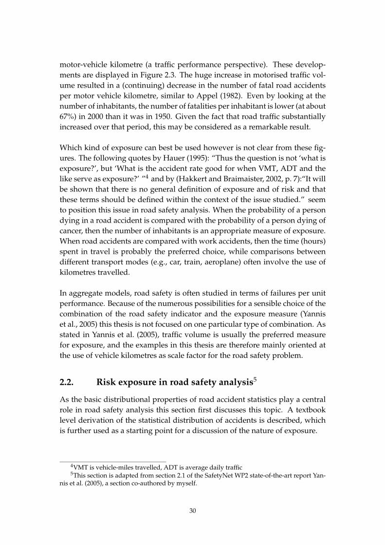
motor-vehicle kilometre (a traffic performance perspective). These develop-
ments are displayed in Figure 2.3. The huge increase in motorised traffic vol-
ume resulted in a (continuing) decrease in the number of fatal road accidents
per motor vehicle kilometre, similar to Appel (1982). Even by looking at the
number of inhabitants, the number of fatalities per inhabitant is lower (at about
67%) in 2000 than it was in 1950. Given the fact that road traffic substantially
increased over that period, this may be considered as a remarkable result.
Which kind of exposure can best be used however is not clear from these fig-
ures. The following quotes by Hauer (1995): “Thus the question is not ‘what is
exposure?’, but ‘What is the accident rate good for when VMT, ADT and the
like serve as exposure?’ ”4 and by (Hakkert and Braimaister, 2002, p. 7):“It will
be shown that there is no general definition of exposure and of risk and that
these terms should be defined within the context of the issue studied.” seem
to position this issue in road safety analysis. When the probability of a person
dying in a road accident is compared with the probability of a person dying of
cancer, then the number of inhabitants is an appropriate measure of exposure.
When road accidents are compared with work accidents, then the time (hours)
spent in travel is probably the preferred choice, while comparisons between
different transport modes (e.g., car, train, aeroplane) often involve the use of
kilometres travelled.
In aggregate models, road safety is often studied in terms of failures per unit
performance. Because of the numerous possibilities for a sensible choice of the
combination of the road safety indicator and the exposure measure (Yannis
et al., 2005) this thesis is not focused on one particular type of combination. As
stated in Yannis et al. (2005), traffic volume is usually the preferred measure
for exposure, and the examples in this thesis are therefore mainly oriented at
the use of vehicle kilometres as scale factor for the road safety problem.
2.2. Risk exposure in road safety analysis5
As the basic distributional properties of road accident statistics play a central
role in road safety analysis this section first discusses this topic. A textbook
level derivation of the statistical distribution of accidents is described, which
is further used as a starting point for a discussion of the nature of exposure.
4VMT is vehicle-miles travelled, ADT is average daily traffic5This section is adapted from section 2.1 of the SafetyNet WP2 state-of-the-art report Yan-
nis et al. (2005), a section co-authored by myself.
30

2.2.1. Statistical distributions
This section is devoted to a discussion of the statistical distribution of aggre-
gated accident counts, with some reference to the distribution of victim counts.
Accident distributions refer to the distribution of the number of accidents and
not to the spatial distribution of the accidents over an area or temporal distri-
bution over time.
An introduction to a discussion of the basic concepts of road accident statistics
is the work by the French mathematician Poisson (see, Feller, 1968, page 153).
Poisson investigated the properties of Bernouilli trials. A Bernouilli trial is an
experiment that has two possible outcomes: success or failure. This type of
experiment seems to be a useful building block for modelling road safety. For
instance, the crossing of a road by a pedestrian can be conceived of as an exper-
iment with a (fortunately) minimal probability of a ‘success’ (i.e., an accident
occurring). A similar argument could be used for a vehicle passing through
a road section, a vehicle driving past a road side obstacle, or two vehicles en-
countering each other on the road. Many other examples could be considered.
The concept of a trial in this chapter is different from the concept of a conflict in
Hauer (1982), which is at a much later – almost final – stage of the development
of an accident.
The original work of Poisson assumed the probability of success to be the same
at each trial. Poisson could then prove that the distribution of the sum of all
successes would tend to a Poisson distribution. The restriction Poisson used
that the probability of success has to be the same value, say p, at each trial has
since been relaxed (see Feller, 1968, page 282). Let N denote the number of
trials, it is not necessary that all probabilities of success pi are equal to each
other for i = 1, . . . , N. Rather the sum of all N probabilities should tend to a
finite λ (which serves as the expected number of accidents), and its maximum
(e.g. Feller, 1968, page 282) or sum of squares (e.g. Shorack, 2000, page 367)
should tend to nil:
limN→∞
N
∑i=1
pi = λ limN→∞
max1≤i≤N
pi = 0 limN→∞
N
∑i=1
p2i = 0, (2.1)
where N is the number of trials, and pi is the probability of an accident in trial
i.
For the practice of road safety analysis this result has the following conse-
quence: if the number of accidents can be regarded as the sum of the outcomes
of many independent conceptual events, each having a small probability pi of
31

turning into an accident, then the distribution of the sum of those events that
turned into accidents – thus the number of accidents – tends to the Poisson
distribution with parameter equal to the sum of the probabilities of events re-
sulting in an accident. Therefore the expected number of accidents is equal to
the sum of all probabilities, which is λ in the limiting case.
It should be noted that:
1. This result applies to the distribution of the number of accidents, not to
the distribution of the number of victims (unless there happens to be at
most one victim per accident) or of other outcomes of accidents.
2. The role of independence is important in this result. It should be quite
reasonable to assume that the outcomes of the different events are inde-
pendent, otherwise the result may not hold.6
3. When accident registration problems are to be considered, the concept
of ‘a small probability of resulting in an accident’ can be replaced by ‘a
small probability of resulting in an accident and being registered’. The reg-
istration should not be selective.
4. A different but no less important accident registration issue is that usu-
ally only accidents exceeding a certain level of severity are considered. In
that case ‘a small probability of resulting in an accident’ can be replaced
by ‘a small probability of resulting in an accident with a certain severity
and being registered’. Even if these probabilities are different for each
trial, the distribution of the resulting number of accidents still tends to
the Poisson distribution.
5. An alternative approach to deriving the Poisson distribution for counts,
based on counting processes (in real-time), requires that the (real-time)
registration system cannot be saturated by the accident process. Although
this is mostly relevant to Geiger-Muller counter like systems, its potential
effects should not be ignored in road safety analysis. For instance, police
districts may allocate limited resources to less severe accidents, and may
simply stop registering them once a certain threshold is exceeded, thus
truncating distributions.
6Outcomes resulting from the same event, such as the number of persons killed, seriouslyinjured, lightly injured, and unharmed in one accident, are likely to be dependent (see Chap-ter 4 in this thesis, or see, Bijleveld, 2005). Furthermore, it should be noted that it is the eventsthat should be independent, not the probabilities, which may depend on N. Accidents that arecause by other accidents are in most cases considered part of the initial accident.
32
2.2.2. The distribution of accident counts
The statistical properties of accident counts mentioned in the previous section
only apply for large numbers of trials. For road safety analysis this means that
the distribution of accident counts will become indistinguishable from a Pois-
son distribution only in the limiting case. Thus, in practice accident counts will
never be precisely Poisson distributed. The limit character of the properties of
accident counts is due to the large number of trials on which it is based. If a
count is based on many, many trials, it is likely that its distribution is indistin-
guishable from a Poisson distribution. For instance annual, national counts of
a general type of accidents will practically be Poisson distributed. However, a
problem arises when the actual number of trials is not so large. This is the case
when a rare accident type is studied for example, or road sections with small
traffic volumes. For more discussion in the situation in which the number of
trials is not very large, see in particular Lord, Washington, and Ivan (2005).
2.2.3. Over-dispersion
As mentioned in Hauer (2001) over-dispersion is commonly encountered in
road safety analysis: “After the unknown model parameters are estimated,
one usually finds that the accident counts are ‘overdispersed’. That is, that
the differences between the accident counts and model predictions, are larger
than what would be consistent with the assumption that accident counts are
Poisson distributed” (Hauer, 2001, p. 799). This phenomenon also occurs in
settings where one would consider the distribution to be practically identical
to the Poisson distribution. The problem is with the replications used in the
generic model as described by Hauer (2001). Even if the accident distribution
would be indistinguishable from the Poisson distribution, replications would
never be under identical conditions. In other words: replications will be drawn
from a different Poisson distribution each time and the replications will there-
fore vary more than would be expected when the replications are sampled
from the same (Poisson) distribution. A more extensive discussion from the
viewpoint of different probabilities can be found in Lord et al. (2005). See e.g.
Hauer (2001) and the references therein for more on how overdispersion can
be estimated. The methods applied in this thesis never assume the prediction
to be fixed, rather the methods assume the predictions to be subject to error.
This situation is comparable to assuming that “replications would never be
under identical conditions.” as remarked just above. In a general context, this
approach is called a mixture approach to generalised count models, of which
the negative binomial model (a Poisson-Gamma mixture) is one example. In
all cases in this thesis it appears that no overdispersion parameter in addition
to the mixture needs to be estimated. The approach where the amount of dis-
33

persion in addition to the prediction error is estimated is taken in this thesis.
More general forms and other distributions can be considered in Chapter 7.
2.2.4. Gaussian approximations
The distribution of the number of accidents is often approximated by the Gaus-
sian distribution. This approximation is also used in the models presented in
this thesis, except for those in Chapter 7. The common procedure is to assume
(first approximation) a Poisson distribution with parameter λ, and then to ap-
proximate (second approximation) the Poisson distribution with a Gaussian
distribution with mean parameter and variance parameter equal to λ. In mod-
elling situations, the expected value λ is often estimated by the model predic-
tion of the observed count. When no statistical model is available, the expected
value λ is usually estimated by the observed count. Sometimes an amount of
‘overdispersion’ is added to the variance parameter, that is a constant value is
added to λ.
It should be noted that the approximation of the Poisson distribution by a
Gaussian distribution deteriorates when the accident counts are getting smaller.
There is no general rule as to what value the counts should exceed in order for
the approximation to be sufficiently reliable since that depends on the applica-
tion and the required accuracy. It should also be noted that for many types of
statistical models count data versions are available. Therefore in many cases a
Gaussian approximation is no longer needed.
2.2.5. The distribution of victim counts
Given that an accident occurs, determining the distribution of the number of
victims resulting from that accident is difficult. Obviously the distribution is
dependent on the number of persons involved in that accident7. When done
at all, approximations can be made based on compound distributions. It can
however be assumed that the victim counts are overdispersed, more so than
accident counts. The amount of overdispersion depends on the variation of the
number of victims per accident (see Chapter 4 in this thesis, or Bijleveld, 2005).
This means that victim counts from accidents that rarely involve more than one
victim, will be less ‘extra’ overdispersed than victim counts from accidents that
(more) often involve more than one victim, as compared to the overdispersion
of the number of accidents.
7Which is unfortunately not known in the Netherlands, since unharmed participants in anaccident are not registered unless they are drivers.
34

Generally, the distribution of victim counts has no influence on the distribu-
tion of accident counts. In practice however often accidents exceeding a cer-
tain severity level are registered or used in an analysis. If the distribution of
victim counts changes in a way that the probability of exceeding the severity
level decreases, the expected number of accidents will decrease, and thus the
accident count distribution will change.
2.2.6. The relation between trials and exposure
As discussed above, the number of trials N plays a dominant role in the ex-
pected number of accidents. Assuming the pi values to be sufficiently regular,
the expected number of accidents is proportional to the number of trials since
λN = ∑Ni=1 pi. The number of trials is therefore probably closest to the true
exposure we can get. Unfortunately, the value of N is generally unknown.
Since N and the pi are unknown all need be estimated. Given the fact that es-
timation of each individual pi is impractical, we assume a homogeneous dis-
tribution of the pi. In addition, the data are used in aggregate models, which
means that aggregate counts of accidents are available as well as aggregate es-
timates of exposure. This means that given and estimate of N, only the average
of R (the pi) can be determined.
No general guidelines are available on how to estimate either N or R. As N is
obviously somehow dependent on the scale of road traffic, and the number of
accidents is dependent on both N and R, the approach taken in this thesis is to
estimate both N and R by means of two (approximate, effectively stochastic)
equations:
{
Scale of road traffic ≈ N
Number of accidents ≈ N × R.(2.2)
See Chapter 3 for further details on how N and R are estimated in this the-
sis, an approach which allows for nonlinear relations. The nonlinear nature of
the relations is suggested by the discussion in the next section. Note that (2.2)
implies that any alternative estimate of N proportional to N cannot be distin-
guished from N.
The research question determines for which kind of accident the ‘Number of
accidents’ needs to be analysed. The research question also determines, given
available data, the optimal choice of what quantity can best be used to measure
the ‘Scale of road traffic’ (see also Hauer (1995) and Hakkert and Braimaister
(2002)). All methodology presented in this thesis is independent of choices for
35
‘Number of accidents’ and ‘Scale of road traffic’. However, given the practi-
cal importance of the traffic volume for ‘Scale of road traffic’, the use of traffic
volume as a measure for the scale of road traffic is elaborated upon in the next
section, which discusses the relation between traffic volume and accident oc-
currence from a general and at a less aggregated level.
2.3. Traffic volume and accident occurrence
Traffic volume is a commonly used measure of exposure, and is used in all
examples in this thesis. Therefore some discussion on the relation between
traffic volume and the number of accidents is given in this section.
2.3.1. The relation between ‘traffic volume’ and the number of accidents
In road safety research, many results are obtained from studies using road
sections as observational units. Even when all other variables are held constant
as much as possible, such studies typically reveal a nonlinear relation between
the number of vehicles passing per time unit and the number of accidents or
victims occurring in the same period of time. The number of vehicles passing
a road section per unit of time is linearly related to the traffic volume of a road
section, as its length is fixed. In a formula this can be written as:
number of accidents = f (traffic volume), (2.3)
where f is a (nonlinear) function. Like in Figure 2.4, this function is often in-
creasing as described in the handbook by (Elvik and Vaa, 2004, p. 49). Depend-
ing on the type of accident being studied, however, this function can also be
concave (Hauer, 1995, p. 135), or even decreasing, (see e.g., Hiselius, 2004). Note
that (2.3) could equivalently be defined explaining the number of accidents per
unit road length as a function of traffic intensity (the number of vehicles pass-
ing), rather than traffic volume.
The nonlinear relation is frequently found to be similar to the curved line in
Figure 2.4. A suggested explanation for the general shape of this relation is
that average speed decreases as traffic intensity increases, and the traffic flow
then becomes relatively safer (as expressed by lower pi values in (2.1)). An-
other explanation given is that when road sections are more intensively used,
they get more attention and are therefore designed somewhat safer than other
sections, thus yielding smaller pi values (see for example, p. 11, Reurings and
Janssen, 2006). The latter reasoning only holds when physically different road
sections are compared. Both suggested explanations underline the idea that
36
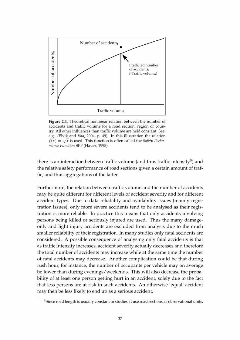
Predicted numberof accidentst
f(Traffic volumet)
Number of accidentst
Traffic volumet
Nu
mb
er o
f ac
cid
ents
t
Figure 2.4. Theoretical nonlinear relation between the number ofaccidents and traffic volume for a road section, region or coun-try. All other influences than traffic volume are held constant. See,e.g. (Elvik and Vaa, 2004, p. 49). In this illustration the relationf (x) =
√x is used. This function is often called the Safety Perfor-
mance Function SPF (Hauer, 1995).
there is an interaction between traffic volume (and thus traffic intensity8) and
the relative safety performance of road sections given a certain amount of traf-
fic, and thus aggregations of the latter.
Furthermore, the relation between traffic volume and the number of accidents
may be quite different for different levels of accident severity and for different
accident types. Due to data reliability and availability issues (mainly regis-
tration issues), only more severe accidents tend to be analysed as their regis-
tration is more reliable. In practice this means that only accidents involving
persons being killed or seriously injured are used. Thus the many damage-
only and light injury accidents are excluded from analysis due to the much
smaller reliability of their registration. In many studies only fatal accidents are
considered. A possible consequence of analysing only fatal accidents is that
as traffic intensity increases, accident severity actually decreases and therefore
the total number of accidents may increase while at the same time the number
of fatal accidents may decrease. Another complication could be that during
rush hour, for instance, the number of occupants per vehicle may on average
be lower than during evenings/weekends. This will also decrease the proba-
bility of at least one person getting hurt in an accident, solely due to the fact
that less persons are at risk in such accidents. An otherwise ‘equal’ accident
may then be less likely to end up as a serious accident.
8Since road length is usually constant in studies at use road sections as observational units.
37

2.3.2. A remark on traffic volume and multiparty accident occurrence
This section briefly addresses the relation between traffic volume and the num-
ber of accidents at a microscopic level in view of multiparty accidents. In 2006,
about two thirds of the fatal accidents in the Netherlands involved more than
one pedestrian or vehicle. This means that it is likely that for substantial part of
the fatal accidents, presence of another vehicle taking part in traffic was some-
how important. The ‘presence’ of another vehicle is probably best understood
as one vehicle or pedestrian being at one point in time in close enough proxim-
ity to be involved in an accident with another vehicle, which may be consid-
ered a ‘trial’. This would mean that for the number of multiparty accidents, the
number of such encounters between vehicles could be more important than the
mere of traffic volume itself. If for instance the number of accidents between
mopeds and cars is to be studied this means that traffic volume of both mopeds
and cars are needed.
This result is plausible because of the fact that an increase in traffic volume
of mopeds is likely to result in an increase in the number of encounters be-
tween mopeds and cars, while an increase in the traffic volume of cars may do
so as well. There is a caveat in that an increase in the traffic volume of cars
on motorways is not likely to have such an effect. To a lesser extent, this issue
is relevant to mopeds as well. Road safety measures tend to separate traffic
flows (separate carriageways for traffic in opposite directions, grade separated
junctions) have similar effects. The ongoing implementation of such measures
systematically tends to alter the relation between traffic volume(s) and acci-
dent occurrence.
It should be noted that the use of two (or more) measures of exposure results
in a different risk concept than when only one measure of exposure is used.
This case is treated in the modelling approach in this thesis in Chapter 5. That
approach maintains the multiplicative interpretation of the risk and exposure
variables in the models.
2.4. Summary and discussion
This chapter discusses two main aspects of road safety: lack of safety and ex-
posure. First lack of safety is discussed. It is assumed that the results of lack
of safety to be used in time series analysis are accident consequences. These
include accident counts and victim counts. It is further noted that the precise
research question determines what type of accidents is to be considered, as is
well known in road safety research. It is important however that accidents
38

are are non-predictable, non-deliberate consequences of entities (vehicles, per-
sons) taking part in traffic.
The well known importance of exposure (or scale) is demonstrated by present-
ing an example that shows that the development of the raw count of fatal acci-
dents in the Netherlands from 1950 to 2000. That development alone may not
sufficiently explain the development of road safety in the Netherlands from
1950 to 2000, as it should then be concluded that little improvement in road
safety was made in 50 years. The development could also suggest that the
road safety situation deteriorated up to the early 1970’s, and then improved
afterwards. However when the number of vehicle kilometres considered (as
an approximate measure of exposure or scale), a different picture emerges.
The use of an exposure measure in combination with an road safety indicator
induces a measure of risk, defined as the road safety indicator per unit of ex-
posure. This chapter discusses established literature considering road safety in
terms of exposure, usually assuming a nonlinear relation, and compares these
approaches to a decomposition of the road safety indicator into exposure and
risk as used further in this thesis.
First, a model for accident occurrence and registration is described based on
encounters between vehicles (including pedestrians). The number of regis-
tered accidents is the number of encounters that resulted in an accident that
is registered. In advanced textbooks it is proven using the limiting behaviour
of sums of Bernouilli trails with unequal probabilities, that under general con-
ditions this sum tends to the Poisson distribution. The underlying number
of encounters is of interest in the discussion considering the relation between
exposure and traffic volume.
It is argued that the expected number of accidents is proportional to exposure.
However, in many road safety studies using road sections as observational
units but also others, nonlinear relations between exposure measures like traf-
fic volume and the number of accidents are found. In such studies however
it is not only traffic volume that changes, but also traffic conditions. Notably,
when traffic volume increases, traffic intensity is likely to increase as well, in
particular when a set of road sections is considered. Therefore, referring to
the accident occurrence model based on Bernouilli trails, it is likely that the
accident probabilities decrease at the same time, as in most but not all cases a
concave function is found. To complicate matters further, it can be argued that
approximate exposure measures like traffic volume are nonlinearly related to
the number of encounters.
39
It is noted that such results are found when it is attempted to hold all other var-
iables constant as much as is possible. When time series models are considered
– in an analysis of road safety data over a longer period of time – this condition
cannot be preserved, because the road safety situation tends to change with
time. Therefore even when a nonlinear relation is know at one time point, it
may have changed in the next. As generally only one observation is available
per time point in time series analysis, it may be impossible to determine the
shape of the nonlinear relation from the data.
This would suggest to adapt (2.2) acknowledging the nonlinear monotone re-
lation between the exposure measure and exposure. Accordingly:
{
Exposure measure ≈ k(N)
Number of accidents ≈ N × R,(2.4)
where k is a nonlinear function, and acknowledge that R may be affected by
exposure. In practical cases k will be strictly monotone, which allows for an
alternative specification:
{
Scale of road traffic ≈ N′
Number of accidents ≈ k−1(N′) × R,(2.5)
where N′ ≡ k(N). The approach (2.5) is taken in this thesis, where N′ is con-
sidered ‘exposure’. Further details, in which time series aspects are considered
can be found in Chapter 3. There it will be demonstrated that in the log lin-
ear modelling context, the important case where k−1(x) is a power function is
absorbed in the model.
40
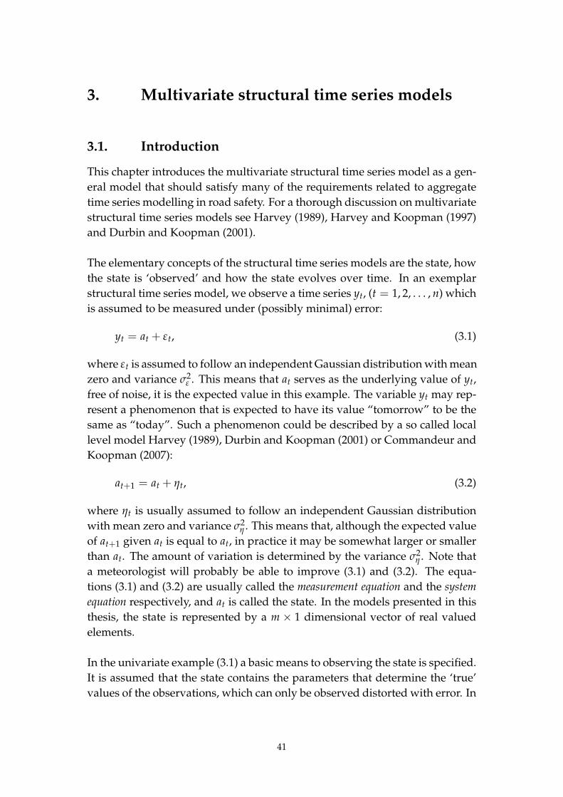
3. Multivariate structural time series models
3.1. Introduction
This chapter introduces the multivariate structural time series model as a gen-
eral model that should satisfy many of the requirements related to aggregate
time series modelling in road safety. For a thorough discussion on multivariate
structural time series models see Harvey (1989), Harvey and Koopman (1997)
and Durbin and Koopman (2001).
The elementary concepts of the structural time series models are the state, how
the state is ‘observed’ and how the state evolves over time. In an exemplar
structural time series model, we observe a time series yt, (t = 1, 2, . . . , n) which
is assumed to be measured under (possibly minimal) error:
yt = at + εt, (3.1)
where εt is assumed to follow an independent Gaussian distribution with mean
zero and variance σ2ε . This means that at serves as the underlying value of yt,
free of noise, it is the expected value in this example. The variable yt may rep-
resent a phenomenon that is expected to have its value “tomorrow” to be the
same as “today”. Such a phenomenon could be described by a so called local
level model Harvey (1989), Durbin and Koopman (2001) or Commandeur and
Koopman (2007):
at+1 = at + ηt, (3.2)
where ηt is usually assumed to follow an independent Gaussian distribution
with mean zero and variance σ2η . This means that, although the expected value
of at+1 given at is equal to at, in practice it may be somewhat larger or smaller
than at. The amount of variation is determined by the variance σ2η . Note that
a meteorologist will probably be able to improve (3.1) and (3.2). The equa-
tions (3.1) and (3.2) are usually called the measurement equation and the system
equation respectively, and at is called the state. In the models presented in this
thesis, the state is represented by a m × 1 dimensional vector of real valued
elements.
In the univariate example (3.1) a basic means to observing the state is specified.
It is assumed that the state contains the parameters that determine the ‘true’
values of the observations, which can only be observed distorted with error. In
41

a multivariate case, which is further developed in this chapter, it is assumed
that apart from error, linear combinations of the state are observed:
yt = Z at + εt, (3.3)
where yt and εt are p × 1 dimensional vectors, and Z is a p × m dimensional
matrix. In Chapter 6 and Chapter 7 a more general form of (3.3) is used. The
concept and measurement of the state is the topic of Section 3.2. Assuming
that the state of road safety in a country evolves over time is empirically sup-
ported, as the road safety situation appears to improve with time. There are
however a number of issues in this respect to be discussed in Section 3.3. This
is done only after the basic measurement structure of the models developed in
this thesis (3.3) is formalised. In that section the basic measurement equations
are formulated using the relation between trials and exposure as described in
Chapter 2. In Section 3.3, the latent risk time series model first formulated,
which is further detailed in Chapter 5, with some example applications in Sec-
tion 3.4. In Section 3.5 some nonlinear extensions are introduced, which are
detailed in Chapter 6 and Chapter 7.
3.2. The concept of state and its observation
When (linear) regression models are applied in road safety analysis, it is as-
sumed that the explanatory variables used in the model (plus all regression
coefficients and possibly an intercept term) sufficiently describe the road safety
outcome. This is what the state in the modelling approach in this thesis is all
about: the state should contain everything that is needed to estimate all the
road safety outcomes. This means that the state may contain both explanatory
variables and coefficients. If some of the explanatory variables are measured
subject to error, it is assumed that the state contains the true values of these
explanatory variables. For instance if it is assumed in a study that seat belt
use is relevant 9 to road safety, then this should be the actual seat belt use, not
the observed percentage of seat belt use obtained from some small (or larger)
survey, which is subject to sampling error. The state may further contain in-
formation on how road safety develops, and thus effectively contains all the
relevant coefficients of a model.
To be more precise, the fundamental assumption of the modelling approach
presented in this thesis is that the ‘state of road safety’ (e.g. in an area, in a
period, in the whole country, for a year) can be described by a finite dimen-
sional vector of data. Two restrictions apply: the first restriction is that the
9A remark on aggregation issues is presented later in this section
42

state vector is assumed to be finite dimensional10 and the second restriction
is that all the state variables are assumed to be real-valued.11 Any observable
quantity, whether being a road safety outcome or an explanatory variable, is
observed through a (potentially trivial) function of the state. This observation
is in general assumed to be subject to (not necessarily independent) random
error.
In a schematic formulation, we have:
road safety outcome ←−g(state) + some random error, (3.4)
while at the same time, for possible explanatory variables we have
explanatory variables ←−h(state) + another random error. (3.5)
Note that the distinction between the multivariate functions g and h is more
conceptual (distinguishing road safety outcomes from explanatory variables)
than practical (g and h together map the unobserved state to the observed
quantities). To stress this distinction between variables, the observed quan-
tities are often called manifest variables, while the unobserved states are often
called latent variables. A schematic representation of these relations between
the observations and the state is also given in Figure 3.1.
In case the full state vector is observable and accurately measured, then ‘an-
other random error’ in (3.5) is zero (which means no error at ‘A’ in Figure 3.1).
Moreover assuming an identity relation for h (meaning that, apart from coef-
ficients, the state simply equals the explanatory variables), (3.5) can be substi-
tuted in (3.4):
road safety outcome ←−g(coefficients, explanatory variables)+
some random error,
which is effectively a classical regression specification. In summary we assume
an observed road safety quantity somehow to be the observation of a particu-
lar state though some function, the observation of which is possibly distorted
10The existence of infinite dimensional models is acknowledged, but such models are notdiscussed. See, e.g. (Chan and Palma, 1998) for an approximation of infinite dimensionalmodels by finite state space models.
11Models using discrete valued state variables, which are used to model processes that mayjump from one state into another (for instance a person changing travel mode in a microscopicmodel) are not discussed.
43
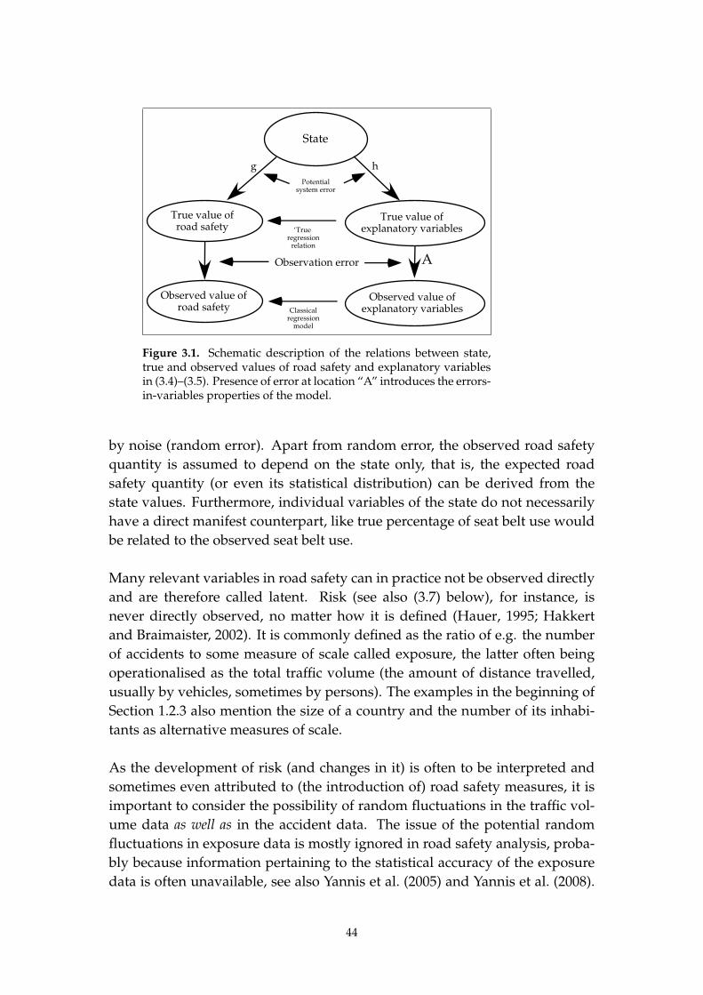
True value ofexplanatory variables
Observed value ofexplanatory variables
Observed value ofroad safety
True value ofroad safety
State
Observation error
Potentialsystem error
Classicalregression
model
g h
‘TrueÕregression
relation
A
Figure 3.1. Schematic description of the relations between state,true and observed values of road safety and explanatory variablesin (3.4)–(3.5). Presence of error at location “A” introduces the errors-in-variables properties of the model.
by noise (random error). Apart from random error, the observed road safety
quantity is assumed to depend on the state only, that is, the expected road
safety quantity (or even its statistical distribution) can be derived from the
state values. Furthermore, individual variables of the state do not necessarily
have a direct manifest counterpart, like true percentage of seat belt use would
be related to the observed seat belt use.
Many relevant variables in road safety can in practice not be observed directly
and are therefore called latent. Risk (see also (3.7) below), for instance, is
never directly observed, no matter how it is defined (Hauer, 1995; Hakkert
and Braimaister, 2002). It is commonly defined as the ratio of e.g. the number
of accidents to some measure of scale called exposure, the latter often being
operationalised as the total traffic volume (the amount of distance travelled,
usually by vehicles, sometimes by persons). The examples in the beginning of
Section 1.2.3 also mention the size of a country and the number of its inhabi-
tants as alternative measures of scale.
As the development of risk (and changes in it) is often to be interpreted and
sometimes even attributed to (the introduction of) road safety measures, it is
important to consider the possibility of random fluctuations in the traffic vol-
ume data as well as in the accident data. The issue of the potential random
fluctuations in exposure data is mostly ignored in road safety analysis, proba-
bly because information pertaining to the statistical accuracy of the exposure
data is often unavailable, see also Yannis et al. (2005) and Yannis et al. (2008).
44

In many cases the consequences of ignoring statistical inaccuracy of traffic vol-
ume data may be negligible compared to other inaccuracies, but such a de-
cision is not always warranted. One example may be the moped travel data
discussed in Section 1.2.3. Further, disaggregated traffic volume data (data for
subgroups) may be subject to substantially larger sampling errors than aggre-
gate data. Other explanatory variables than exposure may also be subject to
random fluctuations. Considering random fluctuations in explanatory varia-
bles as well as in dependent variables implies an ‘errors-in-variables’ approach
(see Seber and Wild, 1988, Chapter 10).
There is no formal requirement with respect to how road safety depends on
the state. In Section 3.3 a log-linear relation is assumed, which appears to be
suitable for many applications. However, some applications require a more
complex relation, as for example discussed in Section 3.5 and Chapter 6 and
Chapter 7.
The state can only define an aggregate estimate of ‘the state of’ road safety, as
it is to represent road safety in a period of time (often a year), for a particular
area (often a country), not the exact conditions of the accidents. This problem is
shared with other aggregate models (almost all other models), like regression
models. This problem is particularly relevant when results from studies at
the accident level are to be incorporated into aggregate (e.g. national) level
models. For instance the temperature at the time of the accident is not likely to
be the average, minimum or maximum temperature of the day, week, month
of year or whatever period of time is used in an analysis. This means that the
level of aggregation has to be considered when results are compared.
As mentioned above, a restriction taken in this thesis is that the state is as-
sumed to be finite dimensional, which excludes certain long range dependency
models. There is evidence of long range dependency in empirical science, al-
though no studies pertaining to this in road safety appear to have been pub-
lished. Koornstra (1992) and Commandeur and Koornstra (2001) have encoun-
tered this phenomenon.
3.3. The latent risk time series model
3.3.1. A basic latent risk observation model
A number of authors have proposed (Hauer, 1995; Hakkert and Braimaister,
2002; see also Section 2.1 in this thesis), that risk can be defined in close re-
lation with the measure of exposure selected as being the most suitable for
45

the purpose of the analysis. Consequently, “risk” is mostly defined to satisfy
“number of accidents” equals “exposure” × “risk”. Therefore, to start a typical
example in a risk analysis setting, a minimal state would consist of an “expo-
sure” variable – in this example assumed to be related to traffic volume – and
a “risk” variable (defined to match this measure of exposure). In this way we
arrive at a situation similar to equation (2.2), which is a simple but common
case of (3.4) and (3.5):
{
Traffic volume = exposure,
Number of accidents = exposure × risk.(3.6)
Having an estimate or observation of the “Traffic volume” and the “Number of
accidents” would yield an estimate of both “exposure” and “risk” by solving
(3.6) for “exposure” and “risk”. If the relations are assumed to be as exact as
in (3.6), then the “risk” estimate is identical to the accident rate “Number of
accidents” divided by “Traffic volume”, as has been done in many studies (e.g,
Oppe, 1991a,c). This means that, although risk cannot be observed, it can still
be measured indirectly.
In the latent risk time series model the approach taken in (3.6) is modified by
applying logarithms on both sides of the equations and subsequently intro-
ducing error terms:
log (Traffic volume) = log (exposure)+
random error in traffic volume,
log (Number of accidents) = log (exposure) + log (risk)+
random error in accidents,
(3.7)
where ‘random error in traffic volume’ is introduced because we assume ‘ex-
posure’ to be only approximately equal to ‘traffic volume’, if only due to ob-
servation error.12
12In addition (3.7) could be modified further by taking the approach suggested in the hand-book by Elvik and Vaa (2004, p 49) by adding a coefficient b:
{
log (Traffic volume) = log (exposure) + random error in traffic volume
log (Number of accidents) = b × log (exposure) + log (risk) + random error in accidents,
(3.8)
an approach which is nested in the modelling approach in this thesis. This is explained inAppendix A.2. Elvik and Vaa (2004, p 49)) define Number of accidents = α Qb. where Q istraffic volume and α is a constant, similar but not equal to risk.
46

The system of equations (3.6) and (3.7) defines a means to estimate the latent
exposure and risk variables from observations of traffic volume and the num-
ber of accidents, where, due to the explicit introduction of error terms, the
estimates have a simultaneous distribution, rather than a fixed point estimate.
It is thus not assumed in advance that traffic volume is identical to exposure
(although it may turn out to be almost similar), hence the presence of the error
terms in the first equation of (3.7). As a result, it is also not assumed in advance
that risk is equal to the number of accidents divided by the traffic volume.
Acknowledging that the actual values of the latent exposure and risk varia-
bles are not accurately known, but that only their statistical distributions are
known, allows a statistical model to improve these estimates by incorporat-
ing estimates of the latent exposure and risk variables based on previous (and
later) time points. How this can be achieved is demonstrated in the following
section.
3.3.2. The role of the dynamic relation among states
Introduction
There are two ways in which time dependence may affect the analysis of road
safety data: the fact that observations are time related, and the fact that de-
pendence between disturbances may affect statistical inference. This section is
devoted to the former aspect. It is generally found that data collected over a
period of time tend to exhibit some form of time dependency (see, e.g. Ham-
pel, Rousseeuw, Ronchetti, and Stahel, 1986, Chapter 8, and many time series
monographs). Ignoring the dependencies may adversely affect the reliability
of statistical tests, and a model should therefore be able to correct for the time
dependencies (see for instance Harvey (1989), Durbin and Koopman (2001) or
Commandeur and Koopman (2007), and Section 3.3.8 for an overview).
The fact that important road safety factors may develop over time implies that
observations close together in time are often more similar than observations
further apart in time. An observation of road safety from 1960 will be less
indicative of the state of road safety in 2000 than an observation of road safety
from 1990.
It should be considered that some and possibly all aspects of a model could
be time-evolving. Conditions in the early days of motorisation are likely to be
different from the current conditions. The introduction of air bags into cars and
the improvement of vehicle construction in general is likely to have influenced
the effectiveness of seat belts in cars, for example. Therefore, the effect of seat
belt use shortly after it became obligatory will not necessarily be the same as
today. This means that some aspect of a model that describes the effectiveness
47

of seat belts is likely to evolve over time. The evolvement of model aspects may
result in slowly changing values of (regression) coefficients. The importance
of the time-evolving nature of a model is of course dependent on the problem
at hand, in particular the length of the analysis period considered. Therefore,
a model should at least allow components to be time evolving. This is one of
the features of the latent risk time series model (LRT) presented in this thesis,
as will be demonstrated below.
For practical purposes, and apart from interventions, it can be assumed that
all aspects of the road safety system develop more or less smoothly (that is:
not completely erratically) over time. The negation of this assumption would
mean that consecutive observations bear no information at all on each other,
similar to assumptions for cross-sectional models. Although the case where
observations bear no information at all on each other is implausible in time
ordered data (see, e.g. Hampel et al., 1986, Chapter 8, and many time se-
ries monographs), it is important that when little information exists between
consecutive observations, models should not be adversely affected by it. See
Appendix A.3 for a further discussion of this issue in reference to multivariate
structural time series models. If absolutely no dynamic relation is assumed
between the time-ordered observations of an explanatory variable, the LRT
allows such variables to be treated similarly to ordinary regression models.
The discussion so far suggests that consecutive observations may be related
and that tendencies may be smooth, but it does not mention how the develop-
ments should be specified. As might be concluded from Figure 3.2, at least as
of the 1970’s, the developments of the log-vehicle kilometres (left hand panel)
and of the log-number of fatal accidents per vehicle kilometre (right hand
panel) may be reasonably well represented by just a straight line. Given the
fact that the points in the figure are the logarithms of the actual observed data,
which are observed subject to random error, one may wonder whether the true
log-exposure and log-risk may not have an even smoother development, pos-
sibly closer to the straight lines in the figure.
Trying to answer this question is the point where the dynamic relation between
the states (exposure and risk) comes into play. If the current year is on average
similar to the previous year and, more generally, if a year can be moderately
well predicted13 from its recent past, how does knowledge of the state of the
13It is important that it on average would predict the next value. The magnitude of thestatistical uncertainty is not important to be allowed to do this, although when the statisticaluncertainty is high compared to the observation uncertainty, using previous observations willnot help much.
48
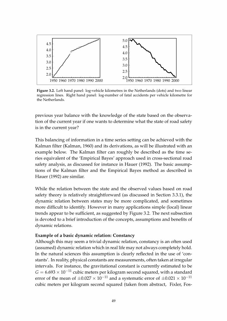
1950 1960 1970 1980 1990 2000
2.0
2.5
3.0
3.5
4.0
4.5
1950 1960 1970 1980 1990 20002.0
2.5
3.0
3.5
4.0
4.5
5.0
Figure 3.2. Left hand panel: log-vehicle kilometres in the Netherlands (dots) and two linearregression lines. Right hand panel: log-number of fatal accidents per vehicle kilometre forthe Netherlands.
previous year balance with the knowledge of the state based on the observa-
tion of the current year if one wants to determine what the state of road safety
is in the current year?
This balancing of information in a time series setting can be achieved with the
Kalman filter (Kalman, 1960) and its derivations, as will be illustrated with an
example below. The Kalman filter can roughly be described as the time se-
ries equivalent of the ‘Empirical Bayes’ approach used in cross-sectional road
safety analysis, as discussed for instance in Hauer (1992). The basic assump-
tions of the Kalman filter and the Empirical Bayes method as described in
Hauer (1992) are similar.
While the relation between the state and the observed values based on road
safety theory is relatively straightforward (as discussed in Section 3.3.1), the
dynamic relation between states may be more complicated, and sometimes
more difficult to identify. However in many applications simple (local) linear
trends appear to be sufficient, as suggested by Figure 3.2. The next subsection
is devoted to a brief introduction of the concepts, assumptions and benefits of
dynamic relations.
Example of a basic dynamic relation: Constancy
Although this may seem a trivial dynamic relation, constancy is an often used
(assumed) dynamic relation which in real life may not always completely hold.
In the natural sciences this assumption is clearly reflected in the use of ‘con-
stants’. In reality, physical constants are measurements, often taken at irregular
intervals. For instance, the gravitational constant is currently estimated to be
G = 6.693 × 10⁻¹¹ cubic meters per kilogram second squared, with a standard
error of the mean of ±0.027 × 10⁻¹¹ and a systematic error of ±0.021 × 10⁻¹¹
cubic meters per kilogram second squared (taken from abstract, Fixler, Fos-
49

ter, McGuirk, and Kasevich, 2007). This value of the gravitational constant is
commonly substituted in equations. Because their development is practically
constant and their measurement sufficiently accurate for most purposes, their
‘state estimate’ can be assumed to be a constant value too for most applica-
tions. This substituting of values in equations is roughly how the LRT treats
missing values in data, as will be detailed later below.
Constancy as a dynamic relation can be specified as follows:
{
yt = a + εt,
at = at−1,(3.9)
for t = 1, . . . , n, where yt are the observations, n is the total number of obser-
vations, a0 = a is the constant state, and εt are the (possibly small) observation
errors.
One application is the computation of the average of a series of data. As an
example, assume that the long run average weight w of sugar lumps produced
in a factory is constant (stated more precisely: the weight of sugar lumps is
independently sampled from a distribution with fixed mean and finite vari-
ance). Every minute one lump is sampled from the production line and the
average weight of the lumps up to that time t, wt is determined. As can be
concluded from limit theorems, the average weight wt will tend to the true
average weight w, but each individual average weight wt, t = 1, 2, . . . will be
slightly different. In the next section it will be demonstrated how this average
can be calculated using the Kalman filter, and how the wt are the so-called fil-
tered estimate of the Kalman filter. The case where the true average weight w
never changes is discussed under the caption ‘Accurate dynamics’ below. The
more realistic case where, due to temperature changes, machine maintenance
and many other reasons, the true average weight w actually changes with time
is discussed under the caption ‘Approximate dynamics’. In the latter case, a
constant value is no longer assumed for the latent state.
The Kalman filter as a algorithm for computing the average of a series of
observations
Accurate dynamics
A simple example of the Kalman filter is the calculation of the average of a se-
ries of identically and independently Gaussian distributed data y1, . . . , yn. This
is a common example where a constant, accurate dynamic relation is assumed.
It is acknowledged that y = (1/n) ∑ni=1 yi is a more familiar and in many cases
50

– but not always – easier way to compute the average of n observations than
the approach described here.
Using the Kalman filter (Kalman, 1960), at the first time point we have y1 = y1
(our first sugar lump). This is what we know about the average if we only have
one observation. At the second time point we have
y2 =1
2y1 +
1
2y2 ≡ y1 + y2
2=
y1 + y2
2,
because y1 and y2 are equally precise estimates of y. The third time point yields
y3 =2
3y2 +
1
3y3 ≡ 2 × y2 + y3
3=
2 × yy+y2
2 + y3
3=
y1 + y2 + y3
3,
and for time point k we have:
yk =k − 1
kyk−1 +
1
kyk. (3.10)
It should be remarked that:
• Although (3.10) may appear unnecessarily complicated, it is efficient in
real-time processing because when a new observation becomes available,
only the weighted sum has to be computed instead of the average of all
(potentially many) observations.
• The approach y = (1/n) ∑ni=1 yi (and the precise implementation in (3.10)
as well) is only optimal when the yi are identically, and to a lesser extent,
Gaussian distributed. Both conditions are not always met. In particular
the condition that the observations should be identically distributed may
often be violated.
As concerns the latter issue, should the observation variances not be all the
same, then the solution is to calculate a weighed average of the sample y1, . . . ,
yn, considering their variances σ2(y1), . . . , σ2(yn) as well. The first (weighted)
average is now (assuming independence):
y2 =σ2(y2)
σ2(y1) + σ2(y2)y1 +
σ2(y1)
σ2(y1) + σ2(y2)y2, σ2(y2) =
σ2(y1)σ2(y2)
σ2(y1) + σ2(y2).
(3.11)
51

Recursively applying this approach thus amounts to applying the Kalman fil-
ter (Kalman, 1960; Harvey, 1981, 1989; Durbin and Koopman, 2001) for the
estimation of the average of a time series. The estimate yk is then called the fil-
tered estimate of y. This approach is almost equivalent to the ‘Empirical Bayes’
approach taken in many road safety studies (e.g. Hauer, 1992, Equation (1),
page 460) except that there the variance for accident counts is estimated differ-
ently from the approach used in Bijleveld (2005) (see also Chapter 4), Bijleveld
et al. (2008) (see also Chapter 5) and Chapter 6.
The filtered state estimate yk is thus an estimate of the state at time k based on
all data up to time k. An alternative estimate of the state is one based on all
available data (not only up to time k), called the smoothed state (Durbin and
Koopman (2001, Chapter 4) for more details). In the simple average example
(3.10), this estimate is equal to y for all time points. In the weighted average
example (3.11) the estimate of the smoothed state also has one and the same
value (i.e., the weighted average) for all time points.
Approximate dynamics
The example above assumes constancy of the estimated quantity. This assump-
tion may be too strict in road safety analysis, particularly when a longer period
of time is considered. Therefore, we have to be careful not to assume a priori too
many values to be constant, although values may well turn out to be constant
in practice. For instance in the drink driving example in Figure 1.4, the alcohol
percentages of drivers exceeding the legal blood alcohol concentration limit
are probably not identical over the whole period, but they may be relatively
constant for some periods.
The LRT approach to this situation is to adapt the estimate (3.10) to a time
varying value by adding a second random component ηt in (3.9),
{
yt = a + εt,
at = at−1 + ηt,
which amounts to modifying the weights according to the now adapted vari-
ances (compare with Hauer, 1992, Equation (1), page 460):
yk = αkyk−1 + (1 − αk)yk, (3.12)
where 0 ≤ αk ≤ 1 and αk is appropriately chosen smaller than (k − 1)/k. The
consequence of this is that the filtered estimate of the state ‘relies’ more on the
actual observation yk than on its prediction from the past yk−1. Hauer (1992,
52

page 460) uses a similar argument. Because of its symmetry, the Kalman fil-
ter approach could be compared to Hauer (1992)’s Empirical Bayes approach
by, in Hauer (1992)’s terminology, considering the observation as the reference
population and the prediction from the previous observation as the ‘accident
count’ or by considering the prediction from the previous observation as the
reference population and the new observation as the ‘accident count’. Both ap-
proaches rely on the fact that if consecutive observations are indeed related (in
Hauer (1992)’s terminology, if we do have a representative reference popula-
tion) then using that information will provide a better estimate. One difference
between the two approaches is that in the LRT, this assumption is extended to
selected explanatory variables as well.
The optimal choice of αk, in (3.12) and its multivariate analogue, is based on
likelihood inference from the Kalman filter (Kalman, 1960; Harvey, 1981, 1989;
Durbin and Koopman, 2001) in Bijleveld et al. (2008) (see Chapter 5) and on
the Extended Kalman Filter (e.g., Harvey, 1989) in Chapter 6 while Chapter 7
relies on a further generalisation of the Kalman filter.
Example of a commonly used dynamic relation: Trend
As mentioned above, it might be concluded from Figure 3.2, at least as of the
1970’s, that the developments of the log-vehicle kilometres (left hand panel)
and of the log-number of fatal accidents per vehicle kilometre (right hand
panel) may be reasonably well represented by just a straight line14, which is
often called a linear trend in time series analysis. The linear regression tech-
niques used to determine the straight lines in the left hand panel of Figure 3.2
assume relations like
log (Traffic volumet) = p × t + q + (some form of random error)t,
where t = 1, 2, . . . , n, q is the intercept or level of the regression line, and p
is the regression coefficient or slope of the regression line. If p × t + q is as-
sumed to be the true value of log (Traffic volumet) (as is usually done in such
models, where – if the model is correct – the prediction is assumed to be a bet-
ter estimate of the observed value than the observed value itself, as under the
model assumptions the observed value is the predicted value plus some form
of random error15), the state variable at representing the ‘true value of expo-
14In this case, where logarithmic transforms of the data are displayed, it appears that theactual data are represented by an exponential line.
15Some multistage analysis techniques, like the DRAG framework by Gaudry (1984) (andJohansson (1996))), use the estimated traffic volume instead of the observed traffic volume.Our approach takes this one step further, as it acknowledges that additional equations simi-larly improve estimates of the true exposure, as well as of other variables.
53

sure’ increments every new time point by the value ‘p’. The trend is specified
by p and q:
at = at−1 + p, a0 = q,
or more generally
{
at = at−1 + pt,
pt = pt−1,a0 = q, p0 = p, t = 1, . . . , n.
When required the LRT approach allows the value of the slope p to change
with time (which would be useful for the modelling of the series in the left
hand panel of Figure 3.2) and/or the value of the level q to change with time
(which would be useful for the modelling of the series in the right hand panel
of Figure 3.2):
{
at = at−1 + pt + η(a)t ,
pt = pt−1 + η(p)t ,
a0 = q, p0 = p, t = 1, . . . , n. (3.13)
Negative values of η(a)t result in a drop in the level q of the trend, which could
be the case in the early 1970’s in the right hand panel of Figure 3.2. Negative
values of η(p)t result in a decrease in the slope p of the trend, with the effect that
the trend increases less fast than before if p is positive, and decreases faster
than before if p is negative. The variances of η(a)t and η
(p)t determine ‘how
easily’ the trend changes. The smaller these variances are, the more the trend
approximates a classical linear trend.
Extreme fluctuations in η(a)t or η
(p)t (as may well occur for η
(p)t around the
1970’s in the left hand panel of Figure 3.2) indicate structural breaks, which
are further discussed in Section 3.3.8. Note that constancy is a special case of
trend.
3.3.3. Specification by means of linear structural models
Introduction
Looking at the observations shown in Figure 3.2, one may be tempted to con-
clude that the log-exposure and log-risk components are simple linear func-
tions of time. However, a closer inspection reveals that this is not precisely
the case, i.e., the developments do not precisely follow a straight line. The
54
log-risk16 in the right hand panel of Figure 3.2, for example, shows a few ‘ups
and downs’ that seem to last longer than just a few years (or observations in
general). The development of the log-risk may therefore well be approximated
by just a linear trend plus some noise in (3.13). The development of the log-
traffic volume in the left hand panel of Figure 3.2 may also reasonably well be
approximated by (two) linear trends, but then some structural break around
1970 will probably be left in the residuals. In addition, it appears that some
cyclic fluctuation around the trend remains. This may (or may not) be an eco-
nomic cycle. The LRT (which is a type of structural time series model) allows
for a kind of building-block approach, where the latent variable for exposure
is decomposed into a linear trend and a cycle component, each having their
own dynamic relation.
The basic idea of the treatment of latent variables in structural models is to de-
compose them into components, sometimes called unobserved components,
that serve special purposes. In this section we follow the introduction of Har-
vey and Shephard (1993) (see also Harvey (1989) and Commandeur and Koop-
man (2007)) and their formulation. These authors propose to decompose a
(univariate) time series yt into a trend (µt), cycle (ψt), seasonal (γt) and irregular
(εt) component:
yt = µt + ψt + γt + εt. (3.14)
As mentioned in Harvey and Shephard (1993), all components are in general
stochastic and their disturbances (see below) are assumed to be mutually un-
correlated (the multivariate case is different in this respect). In order to be
identifiable, the components ψt, γt and εt should on average be nil. In the LRT
approach, which is a multivariate extension of the structural time series mod-
elling approach, there are multiple dependent variables ‘yt’ (traffic volume,
number of accidents) and multiple latent variables ‘µt + ψt + γt’ (exposure,
risk, percentage alcohol abusive drivers, percentage seat belt users, etc). Each
latent variable is represented by the sum of a set of unobserved components.
Such sets of unobserved components may even consist of higher order trends
than linear, multiple seasonal patterns, and multiple cycles, if that should re-
quired for the proper modelling of the dynamic properties of a latent variable.
The trend, seasonal and irregular components are further discussed in the fol-
lowing sections. Cycle components are not used in this thesis, but details can
be found in Harvey (1989, Section 2.3.3) and Harvey and Shephard (1993).
16Note that the log-risk is the logarithm of the empirical risk, thuslog (number of fatal accidents) − log (vehicle kilometres). In the latent risk model fortime series the developments will be smoother.
55

The trend component (local linear trend) µt
As already given in (3.13), the trend specification is:
{
at = at−1 + pt + η(a)t ,
pt = pt−1 + η(p)t ,
a0 = q, p0 = p, t = 1, . . . , n. (3.13)
The component at in (3.13) is called the level component of the trend, and pt
is called the slope component. As the other components (the seasonal and the
irregular discussed below) should be nil on average, the component at serves
as the expected value for yt (compare (3.14)).
If (3.13) describes the trend of exposure, then this will henceforth be denoted
by replacing at by µ(el)t (with ‘l’ for level) and pt by µ
(es)t (with ‘s’ for slope) as
in (3.32). We now have:
(
µ(el)t
µ(es)t
)
=
(
1 1
0 1
) (
µ(el)t−1
µ(es)t−1
)
+
(
η(el)t
η(es)t
)
, (3.15)
which can be rewritten as
αt =
(
1 1
0 1
)
αt−1 + ηt. (3.16)
When the variances of the error terms η(el)t and η
(es)t are nil, (3.15) collapses to
a straight line (see Commandeur and Koopman (2007) for a discussion on how
the linear regression model can be derived from (3.15)). When the variances
of the error terms η(el)t and η
(es)t are not equal to nil, this model is called a
local linear trend model. It can be considered a linear regression model pt ×t + qt, where, if the pt and qt only mildly vary in value over time, the trend
is approximately linear over a short period of time. A trend model where
µ(es)t−1 ≡ 0 is a so-called local level model, an often used special case of a trend.
The seasonal component γt
A second important class of dynamic relation is the seasonal pattern. One
example in Chapter 5 and the example in Chapter 7 include such patterns. The
common approach is to have a – seasonally corrected – trend and an additional
seasonal effect.
In many applications, seasonal patterns are modelled using dummy variables.
When a monthly pattern is to be modelled, effects for each month γ(jan) to γ(dec)
56

are included in a model:
yyear,month = p× year + q + γ(month) + (some form of random error)year,month
(3.17)
where the seasonal pattern also includes the within-year trend, or
yt = p × t + q + γ(month(t)) + (some form of random error)t,
where t increments per month. Neither of these two specifications is fully
determined. To achieve that, many approaches either fix one month at nil, or
enforce γ(jan) + γ(feb) + · · ·+ γ(dec) = 0. The latter approach has the benefit that
the trend component (here simplified to p× t + q) represents the average trend
while in the former approach the trend component represents the trend of the
month fixed at nil. The approach enforcing γ(jan) + γ(feb) + · · · + γ(dec) = 0
is taken17 in structural time series models and the LRT, as it is easily im-
plemented in a dynamic specification, as it implies to enforce e.g. γ(jan) =
−(γ(feb) + · · · + γ(dec)). Thus, the value of the seasonal component for one
month is effectively equal to minus the sum of the last eleven seasonal compo-
nents (where mt(0) is the current month at time t, for instance July and mt(−1)
is June, which also is mt−1(0)):
γ(mt(0))t = −γ
(mt−1(0))t−1 − · · · − γ
(mt−1(−11))t−1 + η
(eγ)t
γ(mt(−1))t = γ
(mt−1(0))t−1
γ(mt(−2))t = γ
(mt−1(−1))t−1
γ(mt(−3))t = γ
(mt−1(−2))t−1
γ(mt(−4))t = γ
(mt−1(−3))t−1
γ(mt(−5))t = γ
(mt−1(−4))t−1
γ(mt(−6))t = γ
(mt−1(−5))t−1
γ(mt(−7))t = γ
(mt−1(−6))t−1
γ(mt(−8))t = γ
(mt−1(−7))t−1
γ(mt(−9))t = γ
(mt−1(−8))t−1
γ(mt(−10))t = γ
(mt−1(−9))t−1 ,
(3.18)
where when t is January, γ(mt(0))t is the effect of January, γ
(mt−1(0))t−1 ≡ γ
(mt(−1))t
is the effect of December last year and γ(mt−1(−1))t−1 is the effect of November
last year. If the variance of η(eγ)t is nil, (3.18) collapses to the classical dummy
17For alternative specifications, see e.g. Harvey (1989).
57

variable approach, as is often used in (generalised) linear models. When the
variance of η(eγ)t is not equal to nil, the seasonal pattern may slowly change
over time.
The system of linear equations (3.18) can also be put into matrix form:
γ(mt(0))t
γ(mt(−1))t
γ(mt(−2))t
γ(mt(−3))t
γ(mt(−4))t
γ(mt(−5))t
γ(mt(−6))t
γ(mt(−7))t
γ(mt(−8))t
γ(mt(−9))t
γ(mt(−10))t
=
η(eγ)t
0
0
0
0
0
0
0
0
0
0
0
+
−1 −1 −1 −1 −1 −1 −1 −1 −1 −1 −1
1 0 0 0 0 0 0 0 0 0 0
0 1 0 0 0 0 0 0 0 0 0
0 0 1 0 0 0 0 0 0 0 0
0 0 0 1 0 0 0 0 0 0 0
0 0 0 0 1 0 0 0 0 0 0
0 0 0 0 0 1 0 0 0 0 0
0 0 0 0 0 0 1 0 0 0 0
0 0 0 0 0 0 0 1 0 0 0
0 0 0 0 0 0 0 0 1 0 0
0 0 0 0 0 0 0 0 0 1 0
γ(mt−1(0))t−1
γ(mt−1(−1))t−1
γ(mt−1(−2))t−1
γ(mt−1(−3))t−1
γ(mt−1(−4))t−1
γ(mt−1(−5))t−1
γ(mt−1(−6))t−1
γ(mt−1(−7))t−1
γ(mt−1(−8))t−1
γ(mt−1(−9))t−1
γ(mt−1(−10))t−1
.
(3.19)
The vector {γ(mt(0))t , . . . , γ
(mt(−10))t }′ thus contains the eleven most recent sea-
sonal effects.
The irregular component εt
The irregular component is similar to the error component in classical regres-
sion models. The irregular components of different time points are assumed
to be independent. However, within each time point, error components are
not necessarily independent. For instance, the number of accidents and the
number of victims are likely to be correlated, as more accidents usually im-
plies more victims as well. As regards traffic volume data, trip data for differ-
58
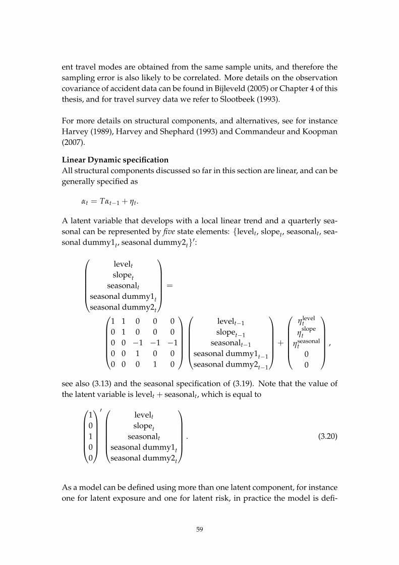
ent travel modes are obtained from the same sample units, and therefore the
sampling error is also likely to be correlated. More details on the observation
covariance of accident data can be found in Bijleveld (2005) or Chapter 4 of this
thesis, and for travel survey data we refer to Slootbeek (1993).
For more details on structural components, and alternatives, see for instance
Harvey (1989), Harvey and Shephard (1993) and Commandeur and Koopman
(2007).
Linear Dynamic specification
All structural components discussed so far in this section are linear, and can be
generally specified as
αt = Tαt−1 + ηt.
A latent variable that develops with a local linear trend and a quarterly sea-
sonal can be represented by five state elements: {levelt, slopet, seasonalt, sea-
sonal dummy1t, seasonal dummy2t}′:
levelt
slopet
seasonalt
seasonal dummy1t
seasonal dummy2t
=
1 1 0 0 0
0 1 0 0 0
0 0 −1 −1 −1
0 0 1 0 0
0 0 0 1 0
levelt−1
slopet−1
seasonalt−1
seasonal dummy1t−1
seasonal dummy2t−1
+
ηlevelt
ηslopet
ηseasonalt
0
0
,
see also (3.13) and the seasonal specification of (3.19). Note that the value of
the latent variable is levelt + seasonalt, which is equal to
1
0
1
0
0
′
levelt
slopet
seasonalt
seasonal dummy1t
seasonal dummy2t
. (3.20)
As a model can be defined using more than one latent component, for instance
one for latent exposure and one for latent risk, in practice the model is defi-
59
ned by stacking the latent components (see also, Chapter 9 Commandeur and
Koopman, 2007). In summary, the dynamic specification of the LRT can be
written as
αt = Tt αt−1 + ct + Rt ηt, (3.21)
where the vector ct can be used to implement effects of explanatory (exoge-
nous) variables, and structural breaks. This vector can also be used to allow
traffic volume to have a direct effect on risk. In the macroscopic models (Oppe,
1989; Oppe and Koornstra, 1990; Oppe, 1991a,c) non-linear (or log-linear) de-
velopments are assumed. Although the methods based on the extended Kalman
filter presented in Chapter 6 could also handle nonlinear dynamic relations,
these are not developed in this thesis, and have not yet been implemented in
the approach presented in Chapter 7.
3.3.4. Linear measurement equations
The latent risk time series model (LRT) is a (multivariate) combination of mea-
surement equations as shown in (3.7), where the components on the right hand
side of (3.7) (the (log-)risk and (log-)exposure components) are assumed to de-
velop over time roughly as discussed in Section 3.3.2, and illustrated with Fig-
ure 3.2.
In this section the measurement model is formalised, and formulated as a set
of linear equations. To this end, more linear equations are added to the set
of linear equations (3.7) discussed in Section 3.4 (and Chapter 5). As a simple
example, the measurement equations in (3.7) can be extended to include victim
counts, as follows:
log (Traffic volume) = log (exposure) + random term1
log (Number of accidents) = log (exposure) + log (risk) + random term2,
log (Number of victims) = log (exposure) + log (risk) + log (injury)+
random term3.
(3.22)
Here ‘log (injury)’ is an additional latent variable describing the (logarithm of)
average number of victims per accident, which may be of interest as a measure
of accident severity. In the remaining of this chapter, a symbolic notation will
be used for the terms in (3.22), including the time index t. From now on, the
log (exposure) is denoted by µ(e)t (where µt stands for a latent variable, and ‘e’
for exposure) with random term ε(e)t , log (risk) is denoted by µ
(a)t (with ‘a’ for
60

accidents) with random term ε(a)t , and log (injury) is denoted by µ
(v)t (‘v’ for
victims) with random term ε(v)t . This yields:
log (Traffic volumet) = µ(e)t + ε
(e)t ,
log (Number of accidentst) = µ(e)t + µ
(a)t + ε
(a)t ,
log (Number of victimst) = µ(e)t + µ
(a)t + µ
(v)t + ε
(v)t .
(3.23)
In matrix notation (3.23) can be written as:
log (Traffic volumet)
log (Number of accidentst)
log (Number of victimst)
=
1 0 0
1 1 0
1 1 1
µ(e)t
µ(a)t
µ(v)t
+
ε(e)t
ε(a)t
ε(v)t
.
Note that a latent variable like µ(e)t may in practice consist of several compo-
nents (such as a level, a slope and a seasonal), and in that case needs to be
represented by a vector. Further letting
yt =
log (Traffic volumet)
log (Number of accidentst)
log (Number of victimst)
, Zt =
1 0 0
1 1 0
1 1 1
,
αt =
µ(e)t
µ(a)t
µ(v)t
, εt =
ε(e)t
ε(a)t
ε(v)t
.
(3.23) can be written as
yt = Zt αt + dt + εt, (3.24)
which will be referred to in Section 3.3.5. Just as in the dynamic relation (3.21),
a vector dt is added to allow for explanatory/exogenous variables. Note that
effects included in dt affect how the latent variables are observed. For instance,
in 1994 the survey structure of the travel survey was changed. From then on
under 12 year old inhabitants were included in the survey. This may have had
an effect on some travel indicators. However, there is no reason to assume this
change in the travel survey actually changed travel itself. Therefore the devel-
opment of the latent exposure component µ(e)t should not have been affected,
however, the way it is observed (the survey) did change, so this intervention
should be in the measurement equations.
61

3.3.5. General state space model specification
Combining (3.21) and (3.24) we obtain the full and general specification of the
LRT. The LRT is a linear Gaussian state space model (see e.g., Harvey, 1989;
Durbin and Koopman, 2001) where it is assumed that p× 1 observation vectors
yt (t = 1, . . . , n) are generated by the process:
{
αt = Tt αt−1 + ct + Rt ηt,
yt = Zt αt + dt + εt,ηt ∼ NID(0, Qt), εt ∼ NID(0, Ht) (3.25)
where the error terms εt and ηt are assumed to be zero mean, independent and
identically multivariate Gaussian distributed. The unobserved state at time t
is represented by the m × 1 vector αt. Rt is a selection matrix composed of
r ≤ m columns of the m-dimensional identity matrix Im. The variance matrices
Qt and Ht are assumed to be non-singular (the variance matrix for Rtηt need
not be non-singular). The vectors ct and dt can be used to model effects of
explanatory variables on both the state and the measurement18. In general, the
matrices Zt, Tt, Ht and Qt and vectors ct and dt are assumed to be known or
otherwise to depend on an unknown parameter vector θ. The first equation of
(3.25) is called the state equation, the second equation is called the observation
equation.
In the current context Ht is the sum of a time invariant matrix and a time de-
pendent observation covariance matrix, see alsoBijleveld (2005) or Chapter 4
in this thesis for how this applies to accident data, and Slootbeek (1993) for
how this applies to travel survey data see Slootbeek (1993).
3.3.6. Estimation of parameters and latent factors, missing data
This section discusses the estimation procedure for the linear LRT (see Sec-
tion 5.2 for more details, Section 6.4 for the almost equivalent variant for the
extended Kalman filter, and Section 7.2 for the generalised version). The el-
ements of the unknown parameter vector θ are estimated by the method of
maximum likelihood. For a fully linear model, the Gaussian log-likelihood
function is evaluated by the Kalman filter and numerically maximised with
respect to the unknown parameters, see Harvey (1989) and Durbin and Koop-
man (2001). Consider a state space model with a linear Gaussian observation
18In general, when an explanatory (exogenous) variable affects how road safety is observed,it should be included in dt. If it affects road safety itself, for instance risk, it should be includedin ct.
62
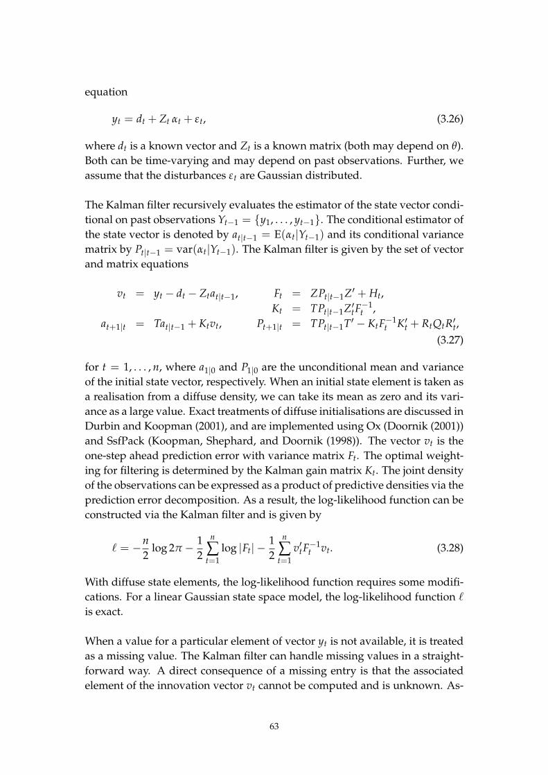
equation
yt = dt + Zt αt + εt, (3.26)
where dt is a known vector and Zt is a known matrix (both may depend on θ).
Both can be time-varying and may depend on past observations. Further, we
assume that the disturbances εt are Gaussian distributed.
The Kalman filter recursively evaluates the estimator of the state vector condi-
tional on past observations Yt−1 = {y1, . . . , yt−1}. The conditional estimator of
the state vector is denoted by at|t−1 = E(αt|Yt−1) and its conditional variance
matrix by Pt|t−1 = var(αt|Yt−1). The Kalman filter is given by the set of vector
and matrix equations
vt = yt − dt − Ztat|t−1, Ft = ZPt|t−1Z′ + Ht,
Kt = TPt|t−1Z′tF
−1t ,
at+1|t = Tat|t−1 + Ktvt, Pt+1|t = TPt|t−1T′ − KtF−1t K′
t + RtQtR′t,
(3.27)
for t = 1, . . . , n, where a1|0 and P1|0 are the unconditional mean and variance
of the initial state vector, respectively. When an initial state element is taken as
a realisation from a diffuse density, we can take its mean as zero and its vari-
ance as a large value. Exact treatments of diffuse initialisations are discussed in
Durbin and Koopman (2001), and are implemented using Ox (Doornik (2001))
and SsfPack (Koopman, Shephard, and Doornik (1998)). The vector vt is the
one-step ahead prediction error with variance matrix Ft. The optimal weight-
ing for filtering is determined by the Kalman gain matrix Kt. The joint density
of the observations can be expressed as a product of predictive densities via the
prediction error decomposition. As a result, the log-likelihood function can be
constructed via the Kalman filter and is given by
ℓ = −n
2log 2π − 1
2
n
∑t=1
log |Ft| −1
2
n
∑t=1
v′tF−1t vt. (3.28)
With diffuse state elements, the log-likelihood function requires some modifi-
cations. For a linear Gaussian state space model, the log-likelihood function ℓ
is exact.
When a value for a particular element of vector yt is not available, it is treated
as a missing value. The Kalman filter can handle missing values in a straight-
forward way. A direct consequence of a missing entry is that the associated
element of the innovation vector vt cannot be computed and is unknown. As-
63

suming that all entries in yt are missing, we treat vt as unknown by taking
vt = 0 and, its variance matrix, Ft → ∞I such that F−1t → 0 and Kt → 0. It
follows that the state update equations can now be written as
at+1|t = Tat|t−1, Pt+1|t = TPt|t−1T′ + RtQtR′t.
These computations are repeated when a number of (consecutive) observa-
tions are missing. This solution also serves as the basis for out-of-sample fore-
casting (where future values are missing) or back-casting (where past values
are missing; this step involves the Kalman smoother as detailed in the next sec-
tion). A missing value does not enter the log-likelihood expression of (3.28).
If only some elements of yt are missing, then the corresponding elements of vt
are taken as zero and the associated rows and columns of F−1t and Kt are taken
as zero vectors (effectively removed).
3.3.7. Kalman smoother, auxiliary residuals
The smoothed estimate of a latent factor is the conditional mean given all avail-
able observations in the sample. The smoothed estimate of the state vector is
denoted by αt = E(αt|Yn) with variance matrix Vt = var(αt|Yn). Once the
Kalman filter has been applied, the smoothed estimates can be computed via
the backward recursions
rt−1 = Z′tF
−1t vt + L′
trt−1, Nt−1 = Z′tF
−1t Zt + L′
tNt−1Lt,
αt = at|t−1 + Pt|t−1rt−1, Vt = Pt|t−1 − Pt|t−1Nt−1Pt|t−1,(3.29)
where Lt = T −KtZt and with initialisations rn = 0 and Nn = 0. The algorithm
is a variation of the fixed interval smoothing method of Anderson and Moore
(1979) and was developed by de Jong (1989) and Kohn and Ansley (1989), see
also Durbin and Koopman (2001, Chapter 4).
3.3.8. Diagnostic checking
Given that the model is well specified, it can be shown that the one-step ahead
prediction error series vt is a Gaussian white noise sequence with variance
matrix Ft, for t = 1, . . . , n. For a set of observation Yn and a given model,
this proposition can be tested via the diagnostic checking of normality, het-
eroscedasticity and serial correlation, see Harvey (1989, Chapter 5).
A particular concern is the existence of outliers and breaks in a time series since
they can distort the estimation of parameters and can be influential in the em-
pirical analysis. Specific diagnostic procedures are developed for the detection
of breaks and outliers in a time series. In the context of state space time series
64

analysis, Harvey and Koopman (1992) and de Jong and Penzer (1998) have
used smoothing errors or so-called auxiliary residuals for this purpose. The
auxiliary residuals are based on the smoothed estimate of the disturbances.
Now
et = F−1t vt − K′
trt, Dt = F−1t + K′
tNtKt,
for t = 1, . . . , n and with rt and Nt computed by (3.29). Note that Dt = var(et)
and Nt = var(rt). A relatively large observation error εt indicates the presence
of an outlier while a relatively large value in the level noise ηt indicates a struc-
tural break, see Harvey and Koopman (1992) for a more detailed discussion.
It is argued by de Jong and Penzer (1998) that such auxiliary residuals can be
computed for any element of the state vector. After standardisation, they can
be considered as t-tests for the hypotheses
H0 : yt − Ztαt − dt − εt = 0, H0 : αt+1 − Tαt − ct − ηt = 0,
element by element, for a particular time point t. The actual statistics for these
hypotheses are given by
e∗it = eit/√
Dii,t, r∗jt = rjt/√
Njj,t, (3.30)
respectively, for i = 1, . . . , N and j = 1, . . . , p, where eit is the ith element
of et, Dii,t is the ith diagonal element of Dt, rjt is the jth element of rt and
Njj,t is the jth diagonal element of Nt. In practice, the diagnostic auxiliary
residual checking procedures are carried out using a conservative significance
level since the interest is limited to serious outliers and breaks, and because
diagnostic checking of the auxiliary residuals involves performing a lot of t-
tests.
3.4. Applications
3.4.1. State space DRAG-similar models
In road safety analysis the demande routiere, accidents et leur gravite (DRAG)
framework of Gaudry (1984) and Gaudry and Lassarre (2000) has been ap-
plied and still is being applied today. The basic form of the DRAG framework
models the dimensions of exposure, risk and severity sequentially. The DRAG
modelling approach consists of three stages: first traffic volume is modelled
(‘demande routiere’). In some applications this is an important step, as often
no true traffic volume data are available (at least not for all data points). In
65

the next step accident frequency (‘des accidents’) is modelled, which is similar to
the risk component of the LRT, and finally severity (‘leur gravite’) is modelled
(the number of fatalities per accident). The LRT approach allows to fit such
models19 using a multivariate unobserved components structure.
In Section 2.2.5 and 2.3 of this thesis we mention that, if accidents are analysed
that are required to exceed a certain severity level, the accident severity level
itself will influence the recorded number of accidents and thus its accident fre-
quency, which implies that the accident risk and accident severity components
could be correlated. Furthermore, as discussed in Bijleveld (2005) and Chap-
ter 4 of this thesis, accident and victim counts (as well as their logarithms) are
also correlated. In this section we therefore propose a DRAG-like model using
a multivariate state space approach, which acknowledges and accommodates
correlations between dependent variables and innovations. The model also
acknowledges the uncertainty in traffic volume data. It may be noted that the
LRT can be regarded as an offspring of the DRAG model. However, it is not
intended to routinely implement Box-Cox transformations as is usual in the
DRAG approach (Box and Cox, 1964; Bickel and Doksum, 1981; Box and Cox,
1982), so the LRT effectively can be considered to be a sub-model of the DRAG
approach. Furthermore no explicit regression coefficients for traffic volume
(exposure) are estimated in the standard LRT, as is discussed in Appendix A.2.
In this section a ‘DRAG’-type version of the LRT is demonstrated using annual
data from the Netherlands. All analyses were also performed on the quar-
terly level (see Commandeur, Bijleveld, and Bergel, 2007, where the results on
quarterly data are presented, also for French networks), but these will not be
discussed here.
The following four dependent variables for t = 1987, . . . , 2005 are used in the
analysis
• Traffic volumet: traffic volume data derived from CBS (2003) and AVV
(2005). The actual data are travel kilometres by drivers in the survey, thus
imitating vehicle kilometres. Note that all drivers in the survey are in-
cluded, also drivers of non-motorised vehicles.
• Accidentst: the number of ‘Killed and seriously injured’ KSI accidents
(according to the police, see Section 3.4.2 for a further example). KSI ac-
cidents are road accidents that have resulted in at least one victim being
19Box-Cox transformations (Box and Cox, 1964; Bickel and Doksum, 1981; Box and Cox,1982) are not implemented in the linear models.
66

killed or seriously injured; in practice seriously injured implies being ad-
mitted into a hospital.20
• KSI victimst: the corresponding number of KSI victims.
• Fatalitiest: the number of fatalities, which is a subset of the KSI victimst.
The dependent variables are assumed to depend on a latent log-exposure var-
iable µ(e)t , a latent log-risk variable µ
(a)t , a latent log-severity variable µ
(k)t serv-
ing as the latent development of the logarithm of the expected number of KSI
victims per KSI accident, and a latent log-lethality variable µ( f )t serving as the
latent development of the logarithm of the expected number of fatalities per
KSI victim. All dependent variables have a random observation error compo-
nent. Each of the latent variables is assumed to develop according to a local
linear trend (see Section 3.3.3). The observation equations are defined as fol-
lows:
log Traffic volumet = µ(e)t + ε
(e)t
log Accidentst = µ(e)t + µ
(a)t + ε
(a)t
log KSI victimst = µ(e)t + µ
(a)t + µ
(k)t + ε
(i)t
log Fatalitiest = µ(e)t + µ
(a)t + µ
(k)t + µ
( f )t + ε
( f )t
(3.31)
The state vector contains the components µ(e)t , µ
(a)t , µ
(k)t and µ
( f )t . Each of these
latent variables follows a local linear trend consisting of a level and a slope
sub-component (there is no seasonal sub-component because we have annual
data). For the latent variable exposure, for example, we have:
µ(e)t ≡
(
µ(el)t
µ(es)t
)
, (3.32)
where (el) (sub-scripted l) denotes the level sub-component associated with
the (e) (for exposure) component. Similarly, (es) (sub-scripted s) denotes the
slope sub-component associated with the (e). The same procedure is followed
for the log-risk component µ(a)t , the latent log-severity variable µ
(k)t , and the
20This category however included victims admitted to hospital for further observation, andreleased the next day considered unharmed.
67

latent log-lethality variable µ( f )t , yielding (see also Section 3.3.3):
statet ≡ αt ≡
µ(e)t
µ(a)t
µ(k)t
µ( f )t
≡
µ(el)t
µ(es)t
µ(al)t
µ(as)t
µ(kl)t
µ(ks)t
µ( fl)t
µ( fs)t
, T =
1 1 0 0 0 0 0 0
0 1 0 0 0 0 0 0
0 0 1 1 0 0 0 0
0 0 0 1 0 0 0 0
0 0 0 0 1 1 0 0
0 0 0 0 0 1 0 0
0 0 0 0 0 0 1 1
0 0 0 0 0 0 0 1
. (3.33)
The following dynamic covariance components are to be estimated:
Q0 =
q11 0 q13 0 q15 0 q17 0
0 q22 0 q24 0 q26 0 q28
q13 0 q33 0 q35 0 q37 0
0 q24 0 q44 0 q46 0 q48
q15 0 q35 0 q55 0 q57 0
0 q26 0 q46 0 q66 0 q68
q17 0 q37 0 q57 0 q77 0
0 q28 0 q48 0 q68 0 q88
, Q = Q′0Q0. (3.34)
The observation vector in (3.25) is
yt ≡
log Traffic volumet
log Accidentst
log KSI victimst
log Fatalitiest
. (3.35)
The observation error covariance matrix Ht is time-variant, and consists of two
parts: a time-variant part based on the results presented in Bijleveld (2005) and
Chapter 4 of this thesis, which is time variant, and a time-invariant part which
is the full covariance matrix for the error due to the model. The observation
matrix Z is set up as:
Z =
1 0 0 0 0 0 0 0
1 0 1 0 0 0 0 0
1 0 1 0 1 0 0 0
1 0 1 0 1 0 1 0
, (3.36)
68

which completes the definition of the vectors and matrices in the general state
space formulation
{
at+1 = T at + ηt
yt = Z at + εt
, ηt ∼ NID(0, Q) εt ∼ NID(0, Ht). (3.37)
The model is applied to two types of data: all accidents and rear-end acci-
dents.21 For both analyses, exponential transforms of the latent log-severity
variable µ(k)t and a latent log-lethality variable µ
( f )t are depicted in Figures 3.3
and 3.4 respectively. From Figures 3.3 and 3.4 it can be inferred that the
confidence intervals of the rear-end accidents are substantially larger than the
confidence intervals for all accidents. This is simply a data issue, as rear-end
accidents are much less frequent than all accidents combined (of which rear-
end accidents are a subset). As a result of this the developments of both com-
ponents associated with the rear-end accidents are much smoother than the
developments of the components associated with all accidents, as the observa-
tion error is relatively larger22. One can argue what can be inferred from these
developments other than some general tendencies. For instance, in Figure 3.3
the development of the number of victims per rear-end accident may appear
to have suddenly increased in the years 1996 and 1997, but it simply cannot
be distinguished from a more gradual increase in the same period (there is
no reason to assume it did either, but that is a different matter). What can be
inferred is that the number of victims per rear-end accident did increase com-
paring the period up to 1995 with the end of the series, although the difference
between the beginning and the end of the series may not be that significant.
It is interesting to see that a similar pattern, but opposite in nature, occurs to
the number of fatalities per victim (Figure 3.4). The rate dropped substantially
21In the latter case no distinction is made between victims travelling in the vehicle impactedin the front (head), in the rear (tail) or in any other vehicle colliding later; all these victims areconsidered simultaneously. However, a model where these distinctions are made could easilybe created as follows:
log Traffic volumet = µ(e)t + ε
(e)t
log Accidentst = µ(e)t + µ
(a)t + ε
(a)t
log KSI victims (head)t = µ(e)t + µ
(a)t + µ
(kh)t + ε
(ih)t
log Fatalities (head)t = µ(e)t + µ
(a)t + µ
(kh)t + µ
( f h)t + ε
( f h)t
log KSI victims (tail)t = µ(e)t + µ
(a)t + µ
(kt)t + ε
(it)t
log Fatalities (tail)t = µ(e)t + µ
(a)t + µ
(kt)t + µ
( f t)t + ε
( f t)t
,
sharing accident occurrence (through µ(e)t + µ
(a)t ), but not its consequences.
22The model tends to ‘follow’ accurate data more closely than (relatively) less accurate data
69
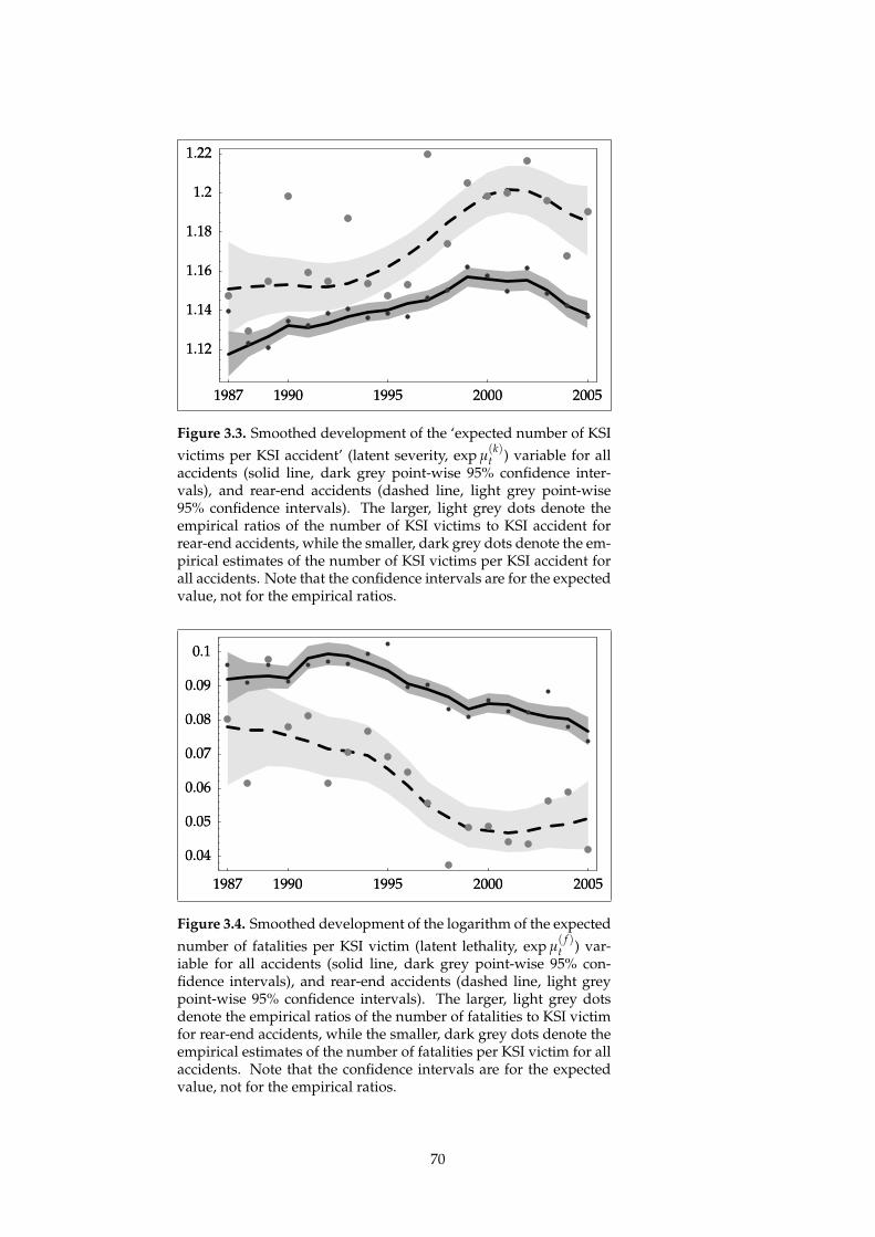
1987 1990 1995 2000 2005
1.12
1.14
1.16
1.18
1.2
1.22
1987 1990 1995 2000 2005
1.12
1.14
1.16
1.18
1.2
1.22
Figure 3.3. Smoothed development of the ‘expected number of KSI
victims per KSI accident’ (latent severity, exp µ(k)t ) variable for all
accidents (solid line, dark grey point-wise 95% confidence inter-vals), and rear-end accidents (dashed line, light grey point-wise95% confidence intervals). The larger, light grey dots denote theempirical ratios of the number of KSI victims to KSI accident forrear-end accidents, while the smaller, dark grey dots denote the em-pirical estimates of the number of KSI victims per KSI accident forall accidents. Note that the confidence intervals are for the expectedvalue, not for the empirical ratios.
1987 1990 1995 2000 2005
0.04
0.05
0.06
0.07
0.08
0.09
0.1
1987 1990 1995 2000 2005
0.04
0.05
0.06
0.07
0.08
0.09
0.1
Figure 3.4. Smoothed development of the logarithm of the expected
number of fatalities per KSI victim (latent lethality, exp µ( f )t ) var-
iable for all accidents (solid line, dark grey point-wise 95% con-fidence intervals), and rear-end accidents (dashed line, light greypoint-wise 95% confidence intervals). The larger, light grey dotsdenote the empirical ratios of the number of fatalities to KSI victimfor rear-end accidents, while the smaller, dark grey dots denote theempirical estimates of the number of fatalities per KSI victim for allaccidents. Note that the confidence intervals are for the expectedvalue, not for the empirical ratios.
70
starting approximately 1994–1995, to a much larger extent than the increase
in the number of victims per accident, resulting in an effective decrease in the
number of fatalities per rear-end accident. Similar results are found for all ac-
cidents, but the decrease in the number of fatalities per accident (for quarterly
data see also, Commandeur et al., 2007) is much slower. Similar results are also
found in the next example, see Figure 3.8 in particular.
3.4.2. Estimating the registration level of accidents involving hospital-
ised victims
In this section an application is presented demonstrating the possibilities of
analysing accident data from different sources. In the Netherlands, the prime
source for accident data is the police registration. However, other sources are
available. The main alternative sources are hospital data (for hospitalised vic-
tims), official mortality statistics and, through surveys (self-reporting). The
police registrations contain the best information on accident circumstances,
while hospital data contain the best information on victim consequences, in
particular in the long-term. However, for a number of reasons, it is not easy to
match hospital data and police data in the Netherlands: it is difficult to match
an individual victim in police records with an individual hospital admission
in the hospital records. Since hospitalised road accident victims are sometimes
missing from police records and because hospitalised victims are sometimes
not correctly identified as road accident victims in hospital records, the ‘true’
figure of hospitalised road accident victims is likely to be larger than both the
number based on hospital records and the number based on police records (see
for more information, Polak, 2000; Reurings, Bos, and van Kampen, 2007).
One particular distinction between police records on the one hand and the hos-
pital records on the other hand is that the former is accident oriented while the
latter is victim oriented. In practice therefore it is almost impossible to de-
termine whether two victims in the hospital records resulted from the same
accident or not. This means that, although studies like Blokpoel and Polak
(1991) and Polak (2000) and Reurings et al. (2007) probably give a good esti-
mate of the actual number of hospitalised road accident victims, without fur-
ther assumptions or information, those studies cannot determine how many
accidents resulted in this number of victims.
The current example demonstrates an approach for estimating this figure. This
is an example intended to demonstrate how this figure could be determined,
and will not yield definitive figures. Currently, studies have started using am-
bulance data (Remmerswaal, 2007), which may result not only in a better link-
ing between police and hospital data but also in information on when and
71

1985 1990 1995 2000 2005 0
5000
10000
15000
20000
25000
1985 1990 1995 2000 2005
54565860626466
Figure 3.5. Left panel: Police and estimated ‘true’ number of hospitalised road accident vic-tims. The number of police registered hospitalised victims is depicted by the solid line. Thedots above this line indicate the ‘true’ number of hospitalised road accident victims basedon studies by Polak (2000) and Reurings et al. (2007). The grey dots indicate data based onextrapolation of previous registration results studies, the black dots indicate actual measure-ments. Right panel: Road accident victim registration level percentage (scale is percentage).The uninterrupted grey line denotes the registration rate based on 100× the number of hos-pitalised victims derived from police data divided by a weighted estimate of the true numberof victims. The dots denote the registration rate based on 100× the number of hospitalisedvictims derived from police data divided by the actual estimate of the true number of victims.
where victims were picked up, thus facilitating the task of matching hospital
data with accidents.
Acknowledging foreseeable future improvements, a LRT model is developed
to estimate the registration level of road accidents involving hospitalised vic-
tims. Note that these accidents do not include fatal victim only accidents, so
they are not equivalent to the KSI accidents of the previous example. In the
left hand panel of Figure 3.5 the number of – police registered – hospitalised
victims is depicted by the solid line. The dots above this line indicate the ‘true’
(actually weighted) number of hospitalised victims based on Polak (2000) and
Reurings et al. (2007). In reality police and hospital data have been matched
only on data from 1985–1986 and 1992–2003 (Polak, 1997; Polak and Blokpoel,
1998; Polak, 2000), resulting in the black dots shown in the figure. Data for
1987–1991 as well as after 2003 are indicated using the grey dots. The data
for these periods were obtained by applying fixed weight factors to subsets of
victims from hospital records and then summing these groups. These weight
factors were based on the 1992–1993 data. This series is commonly used as the
series of the ‘true’ number of hospitalised victims.
Note the substantial difference between the levels of the police registered and
of the ‘true’ number of victims. It is assumed that this difference is mainly
caused due to the police not registering accidents rather than police registering
72

accidents, but missing out on some victims (which does happen, as well as
mixing up on victims).
Apart from the periods with missing data 1987–1991, 2004–2005, an obvious
choice would be to divide the true number of hospitalised victims by the av-
erage number of hospitalised victims per hospitalised victim-accident (a non-
standard accident type). However, the latter figure is similar to the number
of serious victims per KSI accidents as expressed by component µ(k)t in Fig-
ure 3.3), Section 3.4.1, and that component is not time-invariant. Therefore,
analogous to the example in Section 3.4.1, this average number of hospitalised
victims per hospitalised victim-accident is treated as a latent variable.
We use traffic volume data in terms of vehicle kilometres (which include non-
motorised vehicles) in ‘Traffic volumet’, police recorded accident counts of
accidents involving at least one hospitalised victim (according to the police)
in ‘Accidents (police)t’, police recorded hospitalised victims in ‘Hospitalised
(police)t’ and the true number of hospitalised victims in ‘Hospitalised (true)t’,
all for 1985–2005. The LRT consists of the following observation equations:
log Traffic volumet = µ(e)t + ε
(e)t
log Accidents (police)t = µ(e)t + µ
(a)t + µ
(r)t + ε
(ap)t
log Hospitalised (police)t = µ(e)t + µ
(a)t + µ
(h)t + µ
(r)t + ε
(hp)t
log Hospitalised (true)t = µ(e)t + µ
(a)t + µ
(h)t + ε
(ht)t ,
(3.38)
where µ(e)t serves as the latent log-exposure variable, and ε
(e)t is the observa-
tion error component related to traffic volume. Further, µ(a)t serves as the latent
log-accident risk variable, µ(r)t as the latent log-registration rate variable, and
ε(ap)t is the observation error component in the police accident data. Finally,
µ(h)t is the latent log-‘average number of hospitalised victims per hospitalised
victim-accident’ variable, which is shared by both police registered accidents
and ‘hospital registered’ accidents23, ε(hp)t is the observation error component
in the police hospitalised victim data, and ε(ht)t is the observation error com-
ponent in the true number of hospitalised victims. All components µ(e)t , µ
(a)t ,
µ(r)t and µ
(h)t are supposed to develop as local linear trends, as is commonly
assumed in the LRT. Thus the traffic volume depends on exposure, the num-
ber of police recorded accidents depends on exposure, risk and the registration
rate, the number of police recorded hospitalised victims depends on exposure,
23Because it is assumed that the police not registering the accident is the most importantcause of not registering a victim.
73

risk, the registration rate and the number of victims per accident, and the true
number of hospitalised victims finally depends on exposure, risk and the num-
ber of victims per accident.
Almost identically to the previous example, the state vector is now made up
of the components µ(e)t , µ
(a)t , µ
(h)t and µ
(r)t for log-exposure, log-accident risk,
log-‘average number of hospitalised victims per hospitalised victim-accident’
and log-registration rate, which replaces the log-lethality component µ( f )t used
in (3.31). As already mentioned, each of these components is assumed to be a
local linear trend model, and the state vector can therefore be written as:
statet ≡ αt ≡
µ(e)t
µ(a)t
µ(h)t
µ(r)t
≡
µ(el)t
µ(es)t
µ(al)t
µ(as)t
µ(hl)t
µ(hs)t
µ(rl)t
µ(rs)t
. (3.39)
Matrix T is the same as in (3.33) and matrix Q is the same as in (3.34). The
observation vector in (3.38) is:
yt ≡
log Traffic volumet
log Accidents (police)t
log Hospitalised (police)t
log Hospitalised (true)t
. (3.40)
Just as in Section 3.4.1, the observation error covariance matrix Ht is time-
variant, and again consists of two parts: a time-variant part based on the re-
sults presented in Bijleveld (2005) and Chapter 4 of this thesis, which is time-
variant (the ‘hospitalised (true)’ victims are however assumed independent),
and a time-invariant part which is the full covariance matrix for the error due
to the model. The observation matrix Z is now defined as:
Z =
1 0 0 0 0 0 0 0
1 0 1 0 0 0 1 0
1 0 1 0 1 0 1 0
1 0 1 0 1 0 0 0
, (3.41)
74

1985 1990 1995 2000 200550
55
60
65
70
1985 1990 1995 2000 200550
55
60
65
70
Figure 3.6. The smoothed development of the registration rate
for accidents(
100 × exp(
µ(r)t
))
for all data (dashed line) and data
based on actual measurements (ignoring ‘true’ hospitalised victimsfor 1987–1991, 2004 and 2005) (solid line). The dark grey area de-fines the point-wise 95% confidence interval for the registration rate(without 1987–1991, 2004 and 2005), and the light grey area definesthe point-wise 95% confidence interval for the registration rate (in-cluding 1987–1991, 2004 and 2005). The dots denote the registrationrate for hospitalised victims rather than accidents. Note that the twolines are not predictors for the dots in this plot.
which completes the definition of the vectors and matrices in the general state
space formulation (3.37).
Two models are fitted, one using all data, based on the weighted sample, in-
cluding the ‘true’ hospitalised victims for the period 1987–1991 and 2004–2005,
and one based on the actual measurements from the registration studies. The
estimates of the registration rate components (100 × exp(
µ(r)t
)
, for accidents)
obtained in the two analyses are depicted in Figure 3.6, which also contains
the registration rate figures, both for weighted and actual data as presented in
the right hand panel of Figure 3.5. Note that these registration rate figures are
with respect to victims, not accidents.
Although the differences may not be significant, it is clearly visible in Fig-
ure 3.6 that the estimate of the registration rate (ignoring ‘true’ hospitalised
victims for 1987–1991, 2004 and 2005, thus using only actual observations) was
lower than the estimate of the registration rate (including ‘true’ hospitalised
victims for 1987–1991, 2004 and 2005) at the beginning of the series and was
already decaying, probably even before 1985. Obviously, this difference in the
level of the registration rates is caused by the fact that in 1985–1986 the ‘true’
75

1985 1990 1995 2000 2005
5000
10000
15000
20000
25000
Figure 3.7. Dots are the ‘true’ (weighted) number of hospitalisedroad accident victims (including 1987–1991, 2004 and 2005, de-picted in grey, where no real matching is performed). The solid linenear the bottom denotes the police registered hospitalised victim-accidents, the dashed line with light-grey 95% point-wise confi-dence intervals denotes the true number of hospitalised victim-accidents based on weighted data, the solid line with dark-grey 95%point-wise confidence intervals denotes the true number of hospi-talised victim-accidents based on true data from matching studies.
number of victims was larger than the weighted number, and thus the regis-
tration rate was lower (at the end of the series, on the other hand, this situation
is reversed, but the difference there is not significant by any reasonable stan-
dard). Further differences between the two developments may be explained by
the fact that in the 1987–1991 period, only the weighted number of victims has
data. The fact that this is also the case for 2004–2005 does not appear to have a
large impact. It is also visible that the observation for the registration rates of
victims in 1996–1997 are at odds with the other observations. Assuming sim-
ilarity between the registration rate for accidents and victims, this difference
may well be significant. Reurings et al. (2007) also found that this observa-
tion is different from others in other respects. In the end, the differences with
respect to the registration rates between the two approaches are not significant.
In Figure 3.7 the smoothed prediction of the ‘true’ number of hospitalised
victim-accidents is displayed within the context of the police recorded num-
ber of hospitalised victim-accidents and the true number of hospitalised vic-
tims, also displayed in Figure 3.5. Obviously, the differences between the two
approaches are marginal. One concern however is that the differences are sys-
tematic, in that the difference between the weighted and true estimates of the
76

1985 1990 1995 2000 2005
1.08
1.1
1.12
1.14
1.16
1985 1990 1995 2000 2005
1.08
1.1
1.12
1.14
1.16
Figure 3.8. Plot of the number of hospitalised victims per hospi-talised victim-accident (based on weighted data). The dots are the‘true’ (weighted) number of hospitalised victims divided by theestimated true number of hospitalised victim-accidents (based onweighted data model). The dashed line with the light-grey 95%
point-wise confidence intervals denotes exp µ(h)t , the latent ‘average
number of hospitalised victims per hospitalised victim-accident’variable, which is shared by both police registered accidents and‘hospital registered’ accidents, and the solid line with the dark-grey95% point-wise confidence intervals denotes the latent risk varia-
ble exp µ(a)t from (3.31) in the example of Section 3.4.1. Note that
the latter figure also includes fatalities, and is therefore somewhatlarger than the number of hospitalised victims.
number of hospitalised victims is opposite at the beginning and the end of the
series.
In Figure 3.8 the smoothed average number of hospitalised victims per hos-
pitalised victim-accident’ component is compared to an ‘empirical’ estimate.
The development is that the number of hospitalised victims per hospitalised
victim-accident increased up to around the year 2000, and then started to drop
again. A similar pattern (including fatalities in addition to hospitalised vic-
tims) can be observed from police data (solid line, see also (3.31) from the ex-
ample of Section 3.4.1).
3.5. Non linear extensions
3.5.1. Introduction
The latent risk time series model LRT is an additive linear or multiplicative
log-linear model, assuming (at least approximately) Gaussian additive or mul-
77

tiplicative error structures. These assumptions may not always hold. Models
may for instance have both additive and multiplicative components, and in
case of accident counts, may need other error distributions then the Gaussian
distribution.
3.5.2. Mixing additive and multiplicative models
In Chapter 6 a model is presented combining multiplicative and additive mea-
surement equations. The analysis aims to model the disaggregate develop-
ment of road safety inside and outside urban areas. As sometimes happens in
road safety research, disaggregated data are not available for the entire period.
Specifically, although disaggregated accident data are available for the entire
1961 to 2000 period, separate data for traffic volume inside and outside urban
areas are only available in the years 1984 to 1996. This problem is not isolated.
For example, travel data with and without rainfall is generally not available
while this condition is distinguished in accident data (see also Section 3.5.3).
A simplification of the travel survey of the OVG (CBS, 2003) around the year
2000 resulted in certain travel modes becoming more difficult to distinguish
in the survey. A proposed change in the collection of exposure data at Statis-
tics Netherlands may have the opposite effect: certain distinctions that were
previously unavailable may then become available.
In the analysis discussed in Chapter 6 we have the following situation. For
some observations two sets of equations like (3.6) are available,
traffic volume outside urban areas ≈ exposure outside urban areas,
accidents outside urban areas ≈ exposure outside urban areas
×risk outside urban areas,
traffic volume inside urban areas ≈ exposure inside urban areas,
accidents inside urban areas ≈ exposure inside urban areas
×risk inside urban areas,
while for other data points only the total traffic volume is known,
national traffic volume ≈ exposure outside urban areas
+exposure inside urban areas,
accidents outside urban areas ≈ exposure outside urban areas
×risk outside urban areas,
accidents inside urban areas ≈ exposure inside urban areas
×risk inside urban areas.
78

In Chapter 6 of this thesis it is shown how this model can be fitted using the
extended Kalman filter, and by applying local linear trends to both risk and
exposure components of inside and outside urban areas.
3.5.3. Further generalisations
The extended Kalman filter has been improved in some applications. In Chap-
ter 7 of this thesis a generalisation of the Gauss-Newton interpretation of Bell
and Cathey (1993) of the iterated extended Kalman filter (Wishner, Tabaczyn-
ski, and Athans, 1969) is presented. The method developed in Chapter 7 ef-
fectively implements the iterated extended Kalman filter when Gaussian er-
rors are assumed, but allows for other statistical distributions, and is capable
of processing large problems. The method is applied in an analysis of daily
data on accidents with and without precipitation and traffic volume. Like in
the previous example (Section 3.5.2) no disaggregated traffic volume with and
without precipitation is available. Unlike the previous example, not even a few
observations with traffic volume with and without precipitation are available.
On the other hand, the traffic related to the accident type (single car accidents)
analysed in Chapter 7 appears moderately affected by rain fall (some results
are available in the literature, but further research would help) so the actual
relative duration of rainfall is – for now – used as a fraction to divide the total
exposure over both weather conditions. Obviously, this indicator cannot be
fully relied upon, so a latent component is used instead.
79
4. The covariance between the number of acci-
dents and the number of victims in multivar-
iate analysis of accident related outcomes24
In this study some statistical issues involved in the simultaneous analysis of accident related
outcomes of the road traffic process are investigated. Since accident related outcomes like the
number of victims, fatalities or accidents show interdependencies, their simultaneous analysis
requires that these interdependencies are taken into account. One particular interdependency
is the number of fatal accidents that is always smaller than the number of fatalities as at least
one fatality results from a fatal accident. More generally, when the number of accidents in-
creases, the number of people injured as a result of these accidents will also increase. Since de-
pendencies between accident related outcomes are reflected in the variance-covariance struc-
ture of the outcomes, the main focus of the present study is on establishing this structure. As
this study shows it is possible to derive relatively simple expressions for estimates of the var-
iances and covariances of (logarithms of) accidents and victim counts. One example reveals a
substantial effect of the inclusion of covariance terms in the estimation of a confidence region
of a mortality rate. The accuracy of the estimated variance-covariance structure of the accident
related outcomes is evaluated using samples of real life accident data from the Netherlands.
Additionally, the effect of small expected counts on the variance estimate of the logarithm of
the counts is investigated.
4.1. Introduction
4.1.1. The need for multivariate modelling of influences on road safety
The development of (road) traffic safety is very often analysed studying the de-
velopment of only one single accident related outcome. However, in practice
there are always several accident related outcomes: the number of accidents
themselves, the number of fatalities, the number of people injured, the cost of
the material damage, and so on. Road safety measures usually do not have
the same (quantitative) effect on each of these accident outcomes. For exam-
ple, it is likely that the compulsory use of seat belts mainly has an effect on
the consequences of an accident, whereas measures aiming to reduce the oc-
currence of drink-driving mainly have an effect on the number of accidents
(and therefore on the number of victims). Speed reducing measures are sup-
posed to have an effect on both the number of accidents and the consequences
of an accident. Particular theories, such as for example the risk homeostasis
theory (Wilde, 1994) and the zero risk theory (Summala and Naataanen, 1988)
state that theoretically likely developments may be counteracted because of
behavioural adaptation. An example of this is the use of seat belts which may,
24This chapter appeared as Bijleveld (2005).
80

according to some theories, result in higher speeds and other more dangerous
behaviour, so that the expected reduction in the number of injuries is (at least
partly) undone by the fact that the number of accidents increases.
In order to get a better understanding of the (quantitative) effect of road safety
measures, their potentially differentiated effect on each of the accident related
outcomes should be investigated. This becomes more important when the ef-
fects of different road safety measures introduced in a brief period of time are
to be decomposed. In principle this can often be done by careful definition
of dependent variables using separate univariate models, but in many cases
a multivariate framework, where the dependence between the outcome varia-
bles is acknowledged is likely to be preferable.
The multivariate approach allows for the simultaneous estimation of unknown
quantities based on all relevant data, rather than one estimate per dependent
variable. This feature will become more important as new statistical tech-
niques become practical that allow for unobserved – latent – components. One
example is a multivariate extension of Harvey and Durbin (1986), other ap-
plications include methods like Schafer (1987), that implements an errors-in-
variables approach by means of the EM-algorithm (Dempster et al., 1977) to
generalized linear models by “casting the true covariates as ‘missing data’ ”.
For instance alternative methods exist that estimate a sufficient statistic for the
explanatory variables. One example of an application in road safety is Johans-
son (1996) in which exposure is modelled by means of a latent variable that
is estimated by means of one dependent variable, not all dependent variables
simultaneously. This subject is discussed in more detail in Section 4.4.2.
4.1.2. The issue of dependence among outcomes
One important issue is that multivariate road safety outcomes may not be in-
dependent. A notable example is the fact that no more fatal accidents can occur
in a period of time than the total number of fatalities in that period of time, as
at least one fatality occurs in a fatal accident. A more general example is that
when more road accidents occur in a year than usual, it is likely that more peo-
ple get injured in road traffic as well. The former restriction is not imposed
in this study, rather an approximation is made based on the latter aspect by
developing an expression for the covariance (matrix) of the counts of accident
related outcomes (and logarithms thereof). In some cases it will be possible
to redefine the problem to a problem with independent road safety outcomes.
This will however only simplify matters as far as the off-diagonal elements of
the covariance matrix are concerned. The diagonal elements still have to be
81

estimated in which the covariance matrix is implicitly used. In some cases the
use of multivariate models will be inevitable.
Ignoring the covariance may have serious consequences in inference. Suppose
the differentiated effect of a safety measure is to be evaluated on two different
outcome variables: the annual number of accidents and the annual number of
injured people. Also suppose that two models (A and B, say) are fitted on the
data. For a certain observation (year) it is found that model A overestimates
the observed number of accidents as well as the observed number of injured
by say ten. On the other hand, for the same year model B overestimates the
observed number of accidents also by an amount of ten, but underestimates the
number of injured by an amount of ten. Expressed in terms of ‘fit’ (based on
the assumption that the errors follow a symmetrical but not necessarily normal
distribution) both models are equally likely when the covariance between the
two outcomes is ignored. However, once the positive covariance between the
two outcome variables is taken into account, model A yields a better fit than
model B, as it should. Even worse, if model B overestimates the observed
number of accidents by an amount of ten, but underestimates the number of
injured by an amount of five, then it would yield a better fit than model A if the
covariance between the two outcome variables is ignored. This could possibly
result in false conclusions concerning the differentiated effectiveness of safety
measures.
Thus, in the multivariate analysis (in the sense that multiple outcome variables
are analysed) of road safety the dependencies between the dependent variables
should be taken into account.
4.1.3. An approximating solution
In the following sections an analytical procedure is proposed for the estimation
of the variance-covariance matrix from accident data that can be used in mod-
els based on these moments, such as normal approximations, which includes
the vast majority of available multivariate models in which multiple outcome
variables are analysed.
Some multivariate models for multiple count variables do exist, see
Cameron and Trivedi (1998, Chapter 8). Cameron and Trivedi (1998, p. 252)
however state that “Applications of multivariate count models are relatively
uncommon. Practical experience has been restricted to some special computa-
tionally tractable cases.”
82

For this reason and the fact that accident related outcomes are not restricted
to count data, it is attempted in this paper to define a generally applicable, al-
beit approximate, method for analysing multivariate accident related data that
may work in less tractable cases. To that end, estimates of the mean and co-
variance of those data are developed. It is intended that (possibly derivatives
of) these estimates are used in weighted models based on the normal distri-
bution. The methods will therefore not be suitable for observations based on
a small number of accidents. With respect to the estimates derived in this pa-
per the results in this paper are more extensive than developed in Evans (2003,
par. 3 and appendices). This paper adds expressions for covariance between
outcomes as well as a framework for developing estimates of higher moments,
when needed.
It should be noted that this method differs from methods, for instance in time
series analysis, in which (auto)covariances (of errors) are estimated from within
a model, using aggregated data. The proposed method is different in that it es-
timates covariances from within the accident data, using individual accident
information on the relevant outcomes, for instance the number of victims and
fatalities. Note that in road safety it is rare to have information on non-injured
persons, except for vehicle drivers. In principle it is possible to decide when
the driver of a vehicle is not among the victims and the vehicle was not parked
that the driver probably is a non-injured person. Due to the possible compli-
cations, this possibility is ignored in this study.
Furthermore, only covariances within an observation are estimated in contrast
to for instance time series analysis in which covariances between observations
are estimated.
Recently Hutchings, Knight, and Reading (2003) published a method based on
generalized estimating equations that allows for the estimation of covariances.
The estimation of the covariances is in this case from within a model, but uses
individual accident records. This approach used information on non-injured
car occupants that is not available in many cases including the current study,
where only victims and drivers are registered.
All theory in this study is based on the assumption that accident counts fol-
low a Poisson distribution. At first this seems to be in conflict with modern
theories on generalized Poisson modelling. However, this is not the case. The
Poisson assumption is supported by limit theorems such as Feller (1968, p.
282), of which a less general version can be found in McCullagh and Nelder
(1989, p. 105), concerning the asymptotic distribution of the sum of n (n large)
83

independent Bernoulli trials25 with variable (but quite small) probabilities of
success. If each Bernoulli trial is equivalent to an encounter in road traffic
with a unique but small probability of an accident, the distribution of the total
number of accidents will tend to the Poisson distribution. This result how-
ever neglects the impact the small number of accidents can have on the large
number of encounters.
In practice it is impossible to perform true replications, so the assumption that
accident counts follow a Poisson distribution cannot be verified by means of
an experiment. Observations that are assumed to be replications in practice pro-
duce larger variation than can be explained by the Poisson distribution. This
is by no means a disproof of the assumption. More on causes of this overdis-
persion phenomenon can be found in Hauer (2001). In these cases however,
it is assumed that overdispersion is mostly a modelling issue rather that a data
issue. As described in Section 4.4.2 this approach of overdispersion can also be
taken using this study.
In contrast to the strict assumptions on the accident counts, the assumptions on
the distribution of the outcomes are rather relaxed. It is assumed that the mo-
ments of the variables that are a consequence of the accident (e.g. the number
of victims, cost of damage) is finite. This assumption will in practice always
be met as in practice damage is limited. Additionally it is assumed that the
outcomes are independently and identically distributed for all accidents. It is
likely that the results can be extended to not identically distributed outcomes.
The fact that the proposed method uses information on individual accidents
will prohibit its use in cases where only aggregated accident information is
available.
4.1.4. Overview of the paper
Section 4.2 describes and discusses the results of an analytical derivation of
the covariance between the total number of accidents (not necessarily injury
accidents) and the total number of victims in a time period. The latter could
also have been the total cost of damages or any other measurable quantity
resulting as a consequence of an accident. The analytical results can be used to
derive higher order moments than covariances as well.
25A Bernoulli trial with parameter p is an experiment with probability p of ‘success’ (unfor-tunately an accident in this case) and probability 1 − p of ‘failure’ (no accident)
84

The analytical results are compared with results based on simulation in Sec-
tion 4.3. This is done using samples from real accident data from the Nether-
lands in the period 1980–1999. The purpose of this is to assess the accuracy of
the variance-covariance estimates based on the analytical derivations. Simula-
tion studies have been performed on four sets of accidents: the first set consists
of fatal car-only accidents, in the second set injury only accidents are included
as well, the third set consists of fatal accidents (not just car-only accidents) and
in the fourth injury accidents are included.
In Section 4.4 some examples are discussed of (possible) applications of the
methods.
4.2. The covariance structure of road safety related
outcomes
4.2.1. Introduction
This section describes how an estimate of the covariance matrix of the number
of (injury) accidents and victims can be computed. In the following ‘number
of victims’ may be read as ‘the cost of damage’ or any other consequence of an
accident, as long as this consequence is equally and independently distributed
with finite moments for all accidents. Details on the derivations can be found
in the appendix.
4.2.2. Results
Using the results of the derivations reported in the appendix, variance-covari-
ance estimates are formulated between either the count variables or the loga-
rithms of those count variables. As stated above, these results are applicable
to any variable with finite moments that is the consequence of an accident.
Two cases are developed in this study: the total number of accidents, victims
and fatalities and the logarithm of the total number of accidents, victims and
fatalities.
Table 4.2 provides an overview of all results while Table 4.1 contains an expla-
nation of abbreviations used in Table 4.2.
Table 4.1 shows that not all information is available in standard publications on
accidents. This is indicated by a “*”. Detailed sources on individual accidents
are needed to get more precise estimates. In that case probably the individual
85

Number of:Realisation Abbreviation
accidents (acc) n nvictims in accident i vi
∗
fatalities in accident i fi∗
Sum over all accidents of number of:Estimate Abbrev.
victims (vic) ∑ni=1 vi Σv
fatalities (fat) ∑ni=1 fi Σ f
Sum over all accidents of the square of the number of:Estimate Abbreviation
victims ∑ni=1 v2
i∗ Σv2
fatalities ∑ni=1 f 2
i∗ Σ f 2
Sum over all accidents of the cross product of the numbers of:Estimate Abbreviation
victims and fatalities ∑ni=1 vi fi
∗ Σ f v
Table 4.1. Abbreviations used in the derived equations for variances andcovariances and estimates. The quantities marked ∗ are usually not availablein aggregated accident data.
fatality counts fi and victim counts vi per accident will be available. In that case
for instance the variance of the total number of victims can be computed as the
sum of the squared victims counts as indicated in Table 4.2. It can be seen
that the variance of such victim counts is generally larger than the variance
of similar accident counts. The amount of ‘extra’ variance depends on the
distribution of the number of victims per accident. When more victims tend to
occur in certain types of accident the variance of the number of victims tends
to be higher.
4.3. Simulation studies
To assess the accuracy of the variance-covariance estimates in Section 4.2 a
number of simulation studies were performed. From injury accidents that oc-
curred in the Netherlands in the years 1980 through 1999 the number of victims
and the number of fatalities were recorded for each individual accident as well
as the month and year in which the accident occurred. Additional simulations
were performed using accidents that only involved cars, using accidents that
involved only fatal accidents and using accidents that involved exclusively fa-
tal car-only accidents. All simulation studies were performed by selecting a
86
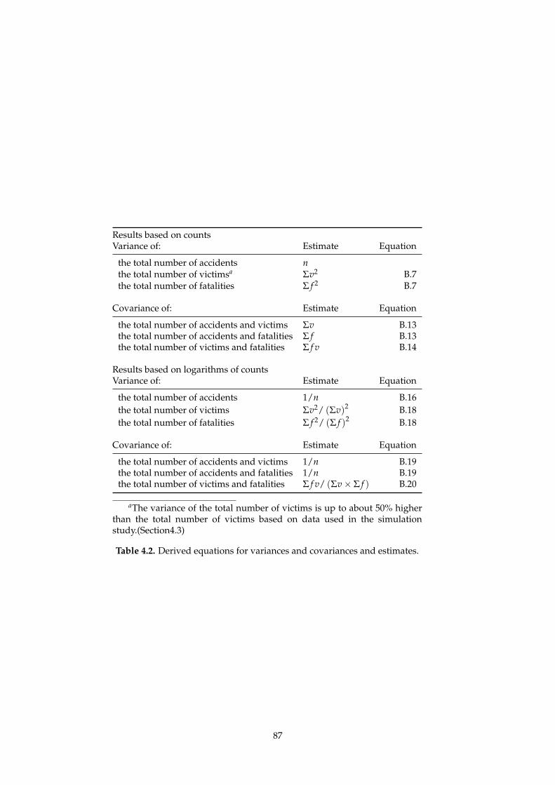
Results based on countsVariance of: Estimate Equation
the total number of accidents nthe total number of victimsa Σv2 B.7the total number of fatalities Σ f 2 B.7
Covariance of: Estimate Equation
the total number of accidents and victims Σv B.13the total number of accidents and fatalities Σ f B.13the total number of victims and fatalities Σ f v B.14
Results based on logarithms of countsVariance of: Estimate Equation
the total number of accidents 1/n B.16
the total number of victims Σv2/ (Σv)2 B.18
the total number of fatalities Σ f 2/ (Σ f )2 B.18
Covariance of: Estimate Equation
the total number of accidents and victims 1/n B.19the total number of accidents and fatalities 1/n B.19the total number of victims and fatalities Σ f v/ (Σv × Σ f ) B.20
aThe variance of the total number of victims is up to about 50% higherthan the total number of victims based on data used in the simulationstudy.(Section4.3)
Table 4.2. Derived equations for variances and covariances and estimates.
87

random number of accident records with replacement from a specific month.
The number of accidents to be selected was a random number sampled from a
Poisson distribution with expected value equal to the number of accidents that
actually occurred that particular month.
This scheme should produce a selection of accidents that could have occurred
almost as likely as the selection of accidents that actually occurred. For each
thus created sample the total number of accidents, victims and fatalities were
computed, as well as the logarithms thereof. Covariances were computed us-
ing a large number of such samples.
Table 4.3 compares results of estimates based on simulations with the estimates
in Table 4.2. The estimates based on simulations were computed as the sam-
ple variance-covariance matrix. Each sample consisted of the 50000 simulated
months. One sample of 50000 was drawn for each of the 240 months in the
range starting january 1980 through december 1999. For each month, sample
estimates (esample) and computed estimates (e) were compared by means of the
difference measure d = (esample − e)/esample.
For each statistic in the first column of Table 4.3 this resulted in 240 difference
measures. The mean values and standard deviations of those 240 difference
measures are listed horizontally in Table 4.3 for each of the four accident selec-
tions. The mean values and standard deviations reflect the amount of similar-
ity between the sample estimates and the computed estimates. A large depar-
ture from zero of a mean value indicates a systematic difference (bias) between
both estimates whereas a relatively large standard deviation is an indication of
inaccuracy of the estimate.
It should be noted that the sampling scheme implies a Poisson distribution of
the number of accidents and therefore simulation checks on the estimation of
the variance of the number of accidents cannot be used to check the variance
estimate. As discussed in the introduction, without true replicates it is im-
possible to validate the Poisson assumption. True replicates would mean for
instance months of traffic sites with exactly the same accident distribution. The
entry ‘var(acc)’ in Table 4.3 is thus for reference only.
Table 4.3 shows that the two types of estimates are quite similar except in the
case of log-fatalities, indicating no important difference between the sample
statistics and the estimates proposed in this study in the other cases. Particu-
larly the logarithmic case with a smaller number of accidents (near the bottom
of Table 4.3) appears to be biased. This bias may be the result of the approx-
88

all all fatal fatalaccidents car accidents accidents car accidents
Measure Mean Std. Mean Std. Mean Std. Mean Std.
var(acc) −0.0000 0.0064 −0.0004 0.0065 0.0004 0.0065 0.0003 0.0063var(vic) −0.0006 0.0062 −0.0002 0.0062 −0.0002 0.0065 0.0004 0.0063var(fat) −0.0001 0.0064 0.0004 0.0066 0.0003 0.0063 0.0004 0.0065cov(acc,vic) −0.0005 0.0067 −0.0005 0.0069 0.0000 0.0069 0.0004 0.0067cov(acc,fat) 0.0006 0.0259 −0.0004 0.0352 0.0003 0.0066 0.0004 0.0066cov(vic,fat) 0.0004 0.0201 0.0006 0.0208 0.0000 0.0068 0.0004 0.0068var(log(acc)) 0.0004 0.0064 0.0021 0.0066 0.0126 0.0078 0.0513 0.0292var(log(vic)) −0.0003 0.0063 0.0023 0.0063 0.0116 0.0099 0.1516 0.1194var(log(fat)) 0.0046 0.0068 0.0687 0.0411 0.0118 0.0076 0.0684 0.0400cov(log(acc),log(vic)) 0.0000 0.0068 0.0026 0.0070 0.0165 0.0087 0.1068 0.0724cov(log(acc),log(fat)) 0.0018 0.0262 0.0164 0.0382 0.0134 0.0079 0.0669 0.0367cov(log(vic),log(fat)) 0.0005 0.0203 0.0123 0.0234 0.0149 0.0083 0.1165 0.0766
Table 4.3. Means and standard deviations of the relative differences(esample − e)/esample between simulation sample estimates of the measures‘esample’ and computed estimates ‘e’, 50000 simulations, based on accidentdata from 1980–1999 in the Netherlands. Abbreviations: var(*)=variance of*, cov(*,#)= covariance of * and #, acc=number of accidents, vic=number ofvictims, fat=number of fatalities, log(*)=logarithm of *.
imation of the logarithm used to obtain an estimate of the variance in these
cases, as it does not occur for instance in the case of var(fat) in combination
with relatively little fatalities. Apparently estimates of the variance may not be
that accurate and care must be taken in case of logarithms in combination with
small counts that these inaccuracies do not influence inferences too much. The
relative error of the variance estimate of the logarithm of a Poisson distributed
random variable is the subject of Section 4.4.3, which is concerned with this
issue.
4.4. Examples
4.4.1. The mortality ratio
As a first application one can use derived statistics as the mortality ratio. The
mortality ratio is the number of fatalities divided by the number of accidents
and as such is an application of multivariate accident related outcomes. In this
example the number of hospitalized victims as well as the fatalities are used.
The ratios are obtained by dividing the number of victims by the number of
accidents resulting in hospitalized victims or worse. Obviously, each ratio is a
nonlinear function of the respective number of victims and the number of ac-
cidents, which themselves are not independent. The textbook approximation
method to this ratio (delta method, see for instance Rice (1995, Chapter 4.6))
is used to obtain the expected value and the variance of the ratio Z = Y/X in
89
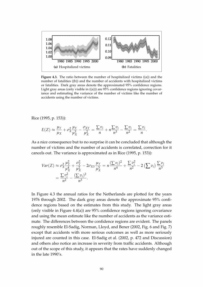
1980 1985 1990 1995 2000
1.001.021.041.061.08
1980 1985 1990 1995 2000
1.001.021.041.061.08
(a) Hospitalized victims
1980 1985 1990 1995 20000.09
0.10
0.11
0.12
1980 1985 1990 1995 20000.09
0.10
0.11
0.12
(b) Fatalities
Figure 4.3. The ratio between the number of hospitalized victims ((a)) and thenumber of fatalities ((b)) and the number of accidents with hospitalized victimsor fatalities. Dark gray areas denote the approximated 95% confidence regions.Light gray areas (only visible in ((a))) are 95% confidence regions ignoring covar-iance and estimating the variance of the number of victims like the number ofaccidents using the number of victims.
Rice (1995, p. 153)):
E(Z) ≈ µY
µX+ σ2
X
µY
µ3X
− σXY
µ2X
=∑ vi
n+ n
∑ vi
n3− ∑ vi
n2=
∑ vi
n.
As a nice consequence but to no surprise it can be concluded that although the
number of victims and the number of accidents is correlated, correction for it
cancels out. The variance is approximated as in Rice (1995, p. 153)):
Var(Z) ≈ σ2X
µ2Y
µ4X
+σ2
Y
µ2X
− 2σXYµY
µ3X
= n(∑ vi)
2
n4+
∑ v2i
n2− 2
(
∑ vi
) ∑ vi
n3
=∑ v2
i
n2− (∑ vi)
2
n3.
In Figure 4.3 the annual ratios for the Netherlands are plotted for the years
1976 through 2002. The dark gray areas denote the approximate 95% confi-
dence regions based on the estimates from this study. The light gray areas
(only visible in Figure 4.4(a)) are 95% confidence regions ignoring covariance
and using the mean estimate like the number of accidents as the variance esti-
mate. The differences between the confidence regions are evident. The panels
roughly resemble El-Sadig, Norman, Lloyd, and Bener (2002, Fig. 6 and Fig. 7)
except that accidents with more serious outcomes as well as more seriously
injured are counted in this case. El-Sadig et al. (2002, p. 472 and Discussion)
and others also notice an increase in severity from traffic accidents. Although
out of the scope of this study, it appears that the rates have suddenly changed
in the late 1990’s.
90

4.4.2. Multivariate state space modelling and the Kalman filter
One possible field of application of the proposed method is in applications
of multivariate time series, for instance using state space models (Durbin and
Koopman, 2001). As stated in the introduction, Johansson (1996, p. 75) ac-
knowledged that the level of exposure is an unobservable variable and in that
study it is modelled as a latent variable. This approach is similar to taken in
Bijleveld, Commandeur, Koopman, and van Montfort (Prep) in which the (ex-
tended) Kalman filter (Harvey, 1989, p. 160) is used to model the development
of the number of fatal accidents inside and outside urban area’s in the Nether-
lands together with vehicle kilometres inside and outside urban area’s. In that
approach it appeared possible to reconstruct the vehicle kilometres inside and
outside urban area’s in years in which only the total (the sum of inside and
outside urban area’s) number of vehicle kilometres is available. The multivar-
iate approach allows for estimation of the latent exposure in Johansson (1996,
p. 75) for all dependent variables, not just on a per dependent variable basis.
That is likely to yield different exposure developments per dependent variable
which may not be optimal.
If counts are modelled linearly in state space models, an additive approach to
overdispersion will be taken. This is due to the way variances are handled in
the Kalman filtering approach. This can be seen from (Durbin and Koopman,
2001p 66, (4.7)) where the prediction error covariance is decomposed into a part
based on the system error (the model part) and an observation part, the latter
composed from the (co)variances of the observation errors, which this study
serves.
4.4.3. The relative error of the variance estimate of the logarithm of a
Poisson distributed random variable
In Section 4.3 it was found that the approximation of the variance of the log-
arithm of counts performs poorly when counts are small. In order to obtain
a better insight into this matter this section is devoted to estimating the error
in approximation. To this end, the theoretical variance of the logarithm of a
Poisson distributed number as a function of its expected value λ is computed
numerically and compared to the estimate 1/λ. Table 4.4 lists the numerical
approximation (s2) of the theoretical variance of the logarithm of a Poisson
distributed number as well as the estimate 1/λ for that number over a range
of small values of the expected value λ of the Poisson distributed number. In
Figure 4.4 the relative difference (approximation-estimate)/approximation is
graphed as a function of the expected value λ. Obviously, both results for
the logarithmic case are approximations, but the numerical approximation is
91

0 5 10 15 20 25 30
-0.2
-0.1
0
0.1
0.2
3.29 6.00
0.231
0.05
Figure 4.4. The relative error of the variance estimate 1/λ of the logarithmof a Poisson distributed random variable with respect to a numerical ap-proximation as a function of the expected value λ of the Poisson distributednumber (horizontal axis). The relative error is computed as (approximation-estimate)/approximation.
much more precise, so all differences are attributed to the estimate. As Fig-
ure 4.4 shows, the relative error for the variance of the number of accidents
can be substantial if λ is less than about 20–30. Similar results will hold for
victims and fatalities, which do not obey a Poisson law but are dependent on
one.
4.5. Conclusions
In this study some statistical issues involved in the simultaneous analysis of
accident related outcomes (such as the number of victims, fatalities or acci-
λ 1/λ s2(Nλ) λ 1/λ s2(Nλ) λ 1/λ s2(Nλ) λ 1/λ s2(Nλ)
1 1.0000 0.1343 11 0.0909 0.1072 21 0.0476 0.0515 31 0.0323 0.03402 0.5000 0.2631 12 0.0833 0.0967 22 0.0455 0.0490 32 0.0313 0.03283 0.3333 0.3037 13 0.0769 0.0881 23 0.0435 0.0467 33 0.0303 0.03184 0.2500 0.2898 14 0.0714 0.0808 24 0.0417 0.0446 34 0.0294 0.03085 0.2000 0.2546 15 0.0667 0.0747 25 0.0400 0.0427 35 0.0286 0.02996 0.1667 0.2168 16 0.0625 0.0695 26 0.0385 0.0409 36 0.0278 0.02907 0.1429 0.1840 17 0.0588 0.0649 27 0.0370 0.0393 37 0.0270 0.02828 0.1250 0.1574 18 0.0556 0.0610 28 0.0357 0.0378 38 0.0263 0.02749 0.1111 0.1366 19 0.0526 0.0574 29 0.0345 0.0364 39 0.0256 0.026710 0.1000 0.1202 20 0.0500 0.0543 30 0.0333 0.0351 40 0.0250 0.0260
Table 4.4. Estimates and approximations of variances of the logarithm of thenumber of accidents when the expected number of accidents is small. Seealso Figure 4.4.
92

dents and costs) of the road traffic process were investigated. The main focus
of this study was on the estimation of the variance-covariance structure of such
outcomes. Correction for covariance is needed in order to enhance the statis-
tical reliability of techniques applied to the simultaneous analysis of accident
related outcomes. It turns out to be possible to derive relatively simple expres-
sions for the variances and covariances of (logarithms of) accidents and victim
counts.
It is argued that when multiple accident outcomes are modelled, their covari-
ance should be taken into account . One example reveals a substantial effect of
the inclusion of covariance terms in the estimation of a confidence region of a
mortality rate.
The variances and covariances were compared with estimates obtained in a
simulation study. Not surprisingly, it was found in the logarithmic case that
bias increases as the number of accidents decreases. In general, estimates will
deteriorate when the number of accidents decreases.
As a special case it is recommended not to use Normal approximations to
the Poisson distribution (Feller, 1968, Chapter VII) of the variance of, for in-
stance, the number of victims in a year by estimating its value using the ob-
served number of victims. The actual variance may be substantially larger.
The amount of ‘extra’ variance depends on the distribution of the number of
victims per accident. When more victims tend to occur in certain types of ac-
cident the variance of the number of victims tends to be higher. As a result
this study confirms that is better to approximate this variance by the sum of
the square of the number of victims per accident rather than by the sum of the
number of victims per accident.
In order to compute the statistics, in some cases information at the level of
individual accidents is needed. For instance the estimate of the variance of
the number of fatalities is computed by summing the squares of the number
of fatalities for each individual accident. This information may not always be
available.
93
5. Model-based measurement of latent risk in
time series with applications26
Risk is at the center of many policy decisions in companies, governments and other institu-
tions. The risk of road fatalities concerns local governments in planning countermeasures, the
risk and severity of counterparty default concerns bank risk managers on a daily basis and
the risk of infection has actuarial and epidemiological consequences. However, risk can not be
observed directly and it usually varies over time. In this paper we introduce a general multi-
variate time series model for the analysis of risk based on latent processes for (i) the exposure
to an event, (ii) the risk of that event occurring and (iii) the severity of the event. Linear state
space methods can be used for the statistical treatment of the model. The new framework is il-
lustrated for time series of insurance claims, credit card purchases and road safety. It is shown
that the general methodology can be effectively used in the assessment of risk.
5.1. Introduction
In the statistics and econometrics literature the term “risk” can take many
meanings. Here we focus on event or operational risk: given a certain level
of exposure, what is the expected severity of loss due to certain events? Exam-
ples of exposure are the number (or value) of buildings owned by a corporate
firm or the size of agricultural land with a certain crop. The event can be fire
(relevant to buildings) and flooding (relevant to crops). This risk definition
contrasts with, for example, Value-at-Risk where the focus is on the maximum
loss with probability of, say, 1% in a prespecified period. These two approaches
of risk can be regarded as complements. Value-at-Risk focuses on the extreme
and total risk while operational risk is concerned with expected and more spe-
cific risk. Government and industry are concerned with a large variety of op-
erational risk in relation to many different events. For example, road safety is
of concern to the general public and therefore most governments take an ac-
tive role in this. Also, insurance companies focus on the risk of a certain claim
while epidemiologic research is usually concerned with medical risk of infec-
tion. There is growing pressure to develop risk models in a range of fields.
International regulations (from the Basel Committee on Bank Supervision) re-
quire banks to be able to model and forecast risk. Road safety researchers have
considerable pressure from governments to evaluate past safety measures and
forecast future accidents and injuries.
Event or operational risk is generally concerned with (i) exposure to an event,
(ii) the probability of the event occurring and (iii) the severity of the event.
26This chapter appeared as Bijleveld, Commandeur, Gould, and Koopman (2008).
94
The time series modelling of event risk offers new insights into data and can
confirm or reject the validity of constant risk assumptions. There is substan-
tial evidence that simple deterministic models fail to adequately explain the
dynamics of risk. Recently a number of articles have examined stochastically
time-varying structures to model risk in epidemiological applications. For ex-
ample, Dominici, McDermott, and Hastie (2004) find evidence of time vary-
ing risk factors within a generalised additive model framework used to deter-
mine the interaction between mortality rates and air pollution concentrations.
Finkenstadt and Grenfell (2000) find evidence of seasonal time variations in a
model for measles epidemics. An illustration of modelling disease incidences
on the basis of latent processes is given by Morton and Finkenstadt (2005). In
actuarial research, there is a surprising lack of time series models for the risk
and severity of insurance claims. Among the few articles is de Jong and Boyle
(1983), in which Bayesian methods are applied to a state space model which
produces stochastically time-varying mortality rates. Harvey and Fernandes
(1989) also develop a model for insurance claims using latent factors where
both the size of claims and the number of claims are modelled. Automobile
insurance claims for multiple cohorts are analysed by Ledolter, Klugman, and
Lee (1991) who test for common latent factors across cohorts. In bank risk man-
agement there have been some articles examining the use of time varying pa-
rameters to model the risk of counterparty default. Allen and Saunders (2003)
highlight the need for dynamic approaches to modelling company default. A
time-varying logistic model for unemployment durations is developed for this
purpose by Fahrmeir and Wagenpfeil (1996). It assesses the probability of sub-
jects entering or leaving a state of unemployment. The results suggest there
is a need for time-variation in model parameters. In road safety research, the
framework of Oppe (1989) assumes that exposure follows a logistic-S curve
and log-risk evolves deterministically. The demande routiere, des accidents et leur
gravite (DRAG) approach of Gaudry (1984) and Gaudry and Lassarre (2000)
uses regression and Box-Jenkins methods for separating the effects of crash
risk and exposure. Li and Kim (2000) use cross-sectional methods for this pur-
pose. Levitt and Porter (2001) show the importance of sample selection in a
micro-economic framework for analysing effects of seatbelts and airbags on
accident survival rates. Time series approaches are regarded as complemen-
tary to cross-sectional methods since they account for serial correlation also
and they can be used when only aggregated time series are available.
In this paper we introduce a general multivariate model for event risk anal-
ysis that can consider exposure, risk and severity simultaneously. The latent
risk time series (LRT) model can be applied to a range of problems involving
event risk and is not specifically limited to particular applications. The LRT
95
model is general and allows for the stochastic evolution of exposure, risk and
severity over time. It extends previous work by treating exposure and severity
as an integral part of the risk problem. In existing approaches some or all of
these variables (particularly exposure) are treated as known, when in reality
they are measured under error and are subject to stochastic variation. The LRT
model has a multivariate structure and therefore correlations between latent
processes and errors can be estimated. The multivariate decomposition can
include latent factors for trend, seasonal and cyclical dynamics together with
regression and intervention effects. It further allows for the forecasting of fu-
ture exposures, events and losses together with prediction confidence bounds,
which are of particular interest to risk managers. Finally, our multivariate
framework also can handle data with multiple cohorts.
The statistical framework, including state space forms and estimation methods
are presented in Section 2. The exposure-risk motor vehicle insurance model is
the first example of a LRT analysis and is discussed in Section 3. The exposure-
risk-severity model for credit card use is treated in Section 4. The multiple
exposure-single risk model for bicycle and moped road traffic accidents is pre-
sented in Section 5. The empirical illustrations include parameter estimation,
signal extraction of latent factors and some discussion of results.
5.2. The statistical framework
The latent risk time series (LRT) model includes latent factors for exposure
Eit, risk Rjt and severity Skt which are associated with the observed varia-
bles exposure Xit, outcome Yjt and the loss Zkt for subject indices i = 1, . . . , I,
j = 1, . . . , J, k = 1, . . . , K and time index t = 1, . . . , n. The basic form of the
model is for I = J = K and links the observables with the latent factors via the
multiplicative relations
Xit = Eit ×U(X)it , Yit = Eit × Rit ×U
(Y)it , Zit = Eit × Rit × Sit ×U
(Z)it ,
where U(a)it are random error terms with unity mean for i = 1, . . . , I, t =
1, . . . , n and a = X, Y, Z. The exposure variable Xit can be the number of ve-
hicle (type i) registrations or distance travelled, the number or value of loans
(type i) or population in region i. The outcome variable Yit is typically the
number of times a certain event occurs for a group i such as claims, accidents
and successful treatments. The loss variable Zit measures the severity of the
outcome such as the dollar value of claims or defaults (type i). The multiplica-
tive error terms reflect that observed variables are measured under uncertainty
due to inaccurate reporting and use of proxy variables. It is not needed to set
96

I = J = K because multiple outcomes for only a single exposure variable can
occur and multiple types of severity can exist for a single outcome. For ex-
ample, we can have multiple types of accidents with cars so that I = 1 and
J > 1.
Variables in logs are denoted by the small version of the corresponding capital
letter used for the original variable, e.g. eit = log Eit. Further, for any t, we
denote vt = (v1t, . . . , vIt)′ where vit represents any variable with two indices i
and t and with the first index i used as stacking argument for i = 1, . . . , I and
t = 1, . . . , n. After taking logs (element by element) and stacking variables in
vectors, the multiplicative LRT equations become the linear system
xt = et + u(x)t , yt = et + rt + u
(y)t , zt = et + rt + st + u
(z)t , (5.1)
where u(a)t is a serially independent disturbance vector with zero mean and
variance matrix Σ(aa)u for a = x, y, z. The disturbances can also be mutually
but instantaneously correlated and the corresponding covariance matrix is de-
noted by Σ(ab)u for a, b = x, y, z and a 6= b. In case the dimension I, J and K do
not match, the different series for x, y and z can be distributed generally via
xt = et + u(x)t , yt = Hyxet + rt + u
(y)t , zt = Hzy(Hyxet + rt) + st + u
(z)t ,
(5.2)
where J × I matrix Hyx and K × J matrix Hzy are typically selection matrices
consisting of ones and zeroes. It is assumed that the dimensions of observed
exposure (proxy) x and latent exposure e, of observed outcome y and latent risk
r and of observed loss z and latent severity s match and are equal to I, J and
K, respectively. It is straighforward to modify (5.2) further to account for cases
where the dimensions of observed and corresponding latent variable do not
match. However, identifiability of the system becomes an issue in such cases
while this is not the case for system (5.2) since any latent variable is uniquely
linked with an observed variable.
The additive system (5.1) is the observation equation where log-exposure eit,
log-risk rit and log-severity sit are treated as latent factors which can be mod-
elled separately. The latent factors can be specified as vector autoregressive
integrated moving average (ARIMA) processes. A more flexible approach
is to let these factors depend on a sum of ARIMA processes and fixed ef-
fects as advocated by Harvey (1989), known as structural time series mod-
els, and Bell (2004), known as RegComponent models. For example, latent
97
factor c may partly depend on a trend (long-term) component that is mod-
elled by µ(c)t+1 = µ
(c)t + β
(c)t + η
(c)t with β
(c)t = 0 (local level model) or with
β(c)t+1 = β
(c)t + ζ
(c)t (local linear trend model) where η
(c)t and ζ
(c)t are disturbance
vectors with zero mean and variance matrices Σccη and Σcc
ζ , respectively, for
c = e, r, s. The disturbance vectors η(c)t and ζ
(c)t for latent factor c are mutually
independent. However, the contemporaneous covariance matrix between dis-
turbance vectors η(c)t and η
(d)t , denoted by Σ
(cd)η , can be nonzero for c, d = e, r, s
and c 6= d. This may also apply to ζ(c)t and ζ
(d)t .
In case the time series is observed in quarterly or monthly frequencies, the se-
ries may be subject to seasonal effects. The latent factor c may then depend
on a periodic (seasonal) process that can be modelled by ∑p−1j=0 γ
(c)t+1−j = ω
(c)t
(stochastic seasonal dummy) where γ(c)t is the seasonal effect at time t with
seasonal length p for c = e, r, s. The disturbance vector ω(c)t has similar proper-
ties as the disturbance vectors η(c)t and ζ
(c)t but they are mutually independent
of each other. Apart from trend and seasonal dynamics, latent factors can be
further composed of, possibly stationary, ARIMA processes.
Regression effects can be added to the latent factor as is common within the
frameworks of structural time series models and RegComponent models. Fixed
regression effects can also include intervention effects for outlying observa-
tions D(c)t (τ; 0), level breaks in trend D
(c)t (τ; 1) and slope breaks in trend
D(c)t (τ; 2) where 1 < τ < n is a fixed time point at which the intervention
occurs for factors c = e, r, s. We can formally define the interventions by
D(c)t (τ; 0) = 1, ∆D
(c)t (τ; 1) = 1 and ∆2D
(c)t (τ; 2) = 1 for t = τ, all are zero
otherwise, with difference operator ∆ = 1− B and backshift operator B so that
∆yt = (1 − B)yt = yt − yt−1. An illustration of intervention analysis in this
framework is presented by Harvey and Durbin (1986) for a univariate time
series of road accidents. A general model-based methodology for identifying
interventions from a given time series is developed by de Jong and Penzer
(1998).
Components and fixed effects are assumed to be part of the latent factors et,
rt and st and therefore part of the LRT system. This implies that a seasonal or
an intervention effect in observed exposure also enters the equations for ob-
served outcome and loss. However, the modeller may decide that some effects
need to appear exclusively in one equation. We therefore need to introduce
the idiosyncratic latent factors e(x)t and r
(y)t for the observation equations for
98

exposure and outcome, respectively. We obtain
xt =et + e(x)t + u
(x)t ,
yt =Hyxet + rt + r(y)t + u
(y)t , (5.3)
zt =Hzy(Hyxet + rt) + st + u(z)t .
The compositions of the idiosyncratic factors e(x)t and r
(y)t can be specified in
the same way as the factors et, rt and st as described above. Some account need
to be taken with respect to the identification of the factors. For example, in case
I = J = K = 1, a seasonal component can appear in both et and e(x)t but for the
remaining two equations only one additional seasonal component is available
since only three observed series are given to identify the seasonal effects. This
also applies to other effects that are part of the model.
It is well documented in the literature (see earlier references in this section)
that different linear dynamic processes can be formulated in state space form
jointly. The state equation as formulated in Durbin and Koopman (2001) is
given by
αt+1 = Ttαt + Gtξt, ξt ∼ N(0, Qt), t = 1, . . . , n, (5.4)
where the initial state vector α1 is specified separately. For example, the local
level model defined above is obtained from (5.4) by having Tt and Gt as iden-
tity matrices and setting Qt = Σ(cc)η . Regression effects can also be considered
as a part of the state vector. In this framework we define a component as a
linear function of the state vector containing latent processes and regression
effects. While matrix Gt is typically a known selection matrix, elements of the
matrices Tt and Qt may be unknown as is apparent from the example given
above. The unknown elements are collected in the parameter vector ψ and are
estimated as described below.
The state space formulation is completed with the observation equation
xt
yt
zt
=
FI 0 0 FI 0
Hyx FJ 0 0 FJ
HzyHyx Hzy FK 0 0
θt + ut, θt = Wtαt, t = 1, . . . , n,
(5.5)
with i× i identity matrix Fi for i = I, J, K, signal vector θt = (e′t, r′t, s′t, e(x)′t , r
(y)′t )′
and disturbance vector ut = (u(x)′t , u
(y)′t , u
(z)′t )′. Matrix Wt links the signal θt
99

with the state αt by selecting the appropriate elements of the state vector that
contains the components and fixed regression effects required for modelling
the dependent time series xt, yt and zt.
The state equation (5.4) and the observation equation (5.5) define the state
space model and enables the application of the Kalman filter for the filtering
of the state vector. Filtering refers to the estimation of αt conditional on obser-
vations up to and including time t. Smoothing is similar but the estimation is
conditional on all observations (up to and including time n). A related method
carries out the computations for smoothing. Both methods also compute mean
squared errors for the estimators. In case all disturbances in the model are
normally distributed, we obtain minimum mean squared estimators. When
normality is not assumed, they are minimum mean squared linear estimators.
A textbook treatment of state space methods is given by Durbin and Koop-
man (2001) while a non-technical introduction is given by Commandeur and
Koopman (2007).
The Kalman filter carries out the prediction error decomposition for a given
state space model and a particular value of ψ. This implies that the likelihood
function can be evaluated by the Kalman filter for a given ψ. Maximum like-
lihood estimation of ψ then becomes a standard exercise of numerically max-
imising the likelihood function with respect to ψ. In the empirical applications
of the LRT model below, parameters in ψ are limited to the elements of vari-
ance matrices such as Σ(cc)η given above for the local level model. Regression
coefficients can be placed in the state vector. To ensure positive semi-definite
variance matrices, a variance matrix is decomposed as Σ(cc)η = M′M where M
is a symmetric matrix.
5.3. Case I: a two-dimensional insurance LRT model
The first illustration of the latent risk model concerns insurance policies and
claims related to motor vehicle fatalities in Victoria, Australia. We analyse
annual time series consisting of the number of vehicle registrations (in thou-
sands, exposure xt) and the number of claims (in units, outcome yt) for the
years 1950–2001. Registrations are a measure of the total stock of vehicles on
Victorian roads. The two time series are presented in the upper panels of Fig-
ure 5.1. The registrations series display an upwards, smooth trend while the
fatal claims series have a “hump” shape, with a peak in the early 1970s. Since
registrations have increased monotonically over the past 50 years, the reduc-
tion in fatal claims must have been caused by a decrease in risk. Risk reduc-
100

tions have been driven by gradual improvements in vehicle and road design
together with increased public awareness. Demographic factors have also been
important as a new generation of road users (“baby boomers”) began to start
driving. Public horror at a road casualty toll of 1034 for Victoria in 1970 led to
newspaper declarations of “war on 1034”. This has been indicative of chang-
ing attitudes towards road safety. The effects on attitude have proved to be
long-term. Other important relevant events in the sample are the introduc-
tion of seat belt laws in 1971 and the increased enforcement and mass media
advertising campaigns on road safety in the early 1990s.
1950 1960 1970 1980 1990 2000
1000
2000
3000
1950 1960 1970 1980 1990 2000
500
1000
1950 1960 1970 1980 1990 2000
7
8
1950 1960 1970 1980 1990 2000
-2
-1
0
1950 1960 1970 1980 1990 2000
0.025
0.075
1950 1960 1970 1980 1990 2000
-0.05
0.00
0.05
Figure 5.1. Time series of registered vehicles (in thousands) and crash fatalities (inunits) in Victoria, Australia (row 1). Smooth estimates of exposure (column 1) and risk(column 2) factors modelled as stochastic trends (row 2) with stochastic slopes (row 3)incl. interventions.
The policy exposure series xt and claim outcome series yt are both univariate
(data is not disaggregated into groups or cohorts). A time series for loss zt
(e.g., the dollar value of payouts on claims) is not available and therefore we
consider a two-dimensional LRT model that consists of the first two equations
in (5.3) with Hyx = 1 and with dimensions I = J = 1. The latent factors et and
rt are modelled as local linear trends. The following special events are consid-
ered as intervention variables: (i) in 1970, a publicity campaign was launched
to increase public and governmental awareness of road safety issues (“war on
1034”); (ii) in 1971, introduction of seat belt laws; (iii) in 1980, change in data
collection on vehicle registrations; (iv) in 1990, introduction of advertising and
enforcement initiatives aimed at reducing accident risk; (v) in 1992, another
change in data collection on vehicle registrations. The changes in data collec-
101

tion should only affect exposure and are therefore part of the latent factor et
while the other events should have an effect on risk rt. The intervention (i) is a
long-term effect and therefore captured by a change in the slope term of risk.
The events (ii) and (iv) are taken as immediate step changes in the level of risk.
These interventions are confirmed by applying the methods of de Jong and
Penzer (1998) to this data set. The interventions (i), (ii) and (iv) are assumed
to only have an impact on accident risk, as none of the measures are aimed at
reducing road use.
Estimates for a selection of parameters are displayed in Table 5.2. Standard er-
rors are computed but space considerations prevent us from presenting them.
The estimated (co)variances for trend and slope disturbances for the two latent
factors reveal that exposure and risk are perfectly negatively correlated:
Σ(er)η /
√
Σ(ee)η · Σ
(rr)η = Σ
(er)ζ /
√
Σ(ee)ζ · Σ
(rr)ζ = −1.
The perfect negative correlations mean that both exposure and risk factors are
subject to the same stochastic shocks that determine their time-varying be-
haviour. This finding is in agreement with most road crash research, which
finds a strong negative relationship between risk and exposure. There are a
number of reasons for this relationship, including the fact that roads become
more congested as exposure increases, which slows vehicle speeds such that
fatal or serious injury accidents are less likely. In developed countries, there
has been a period of increased road use and decreasing fatal accident risk over
the past 35 years. Over this period, technology and safety awareness have im-
proved, which is also an indirect cause of the negative correlation. The perfect
correlation of shocks implies that the components can be interpreted as com-
mon factors. Nevertheless, the estimated components are distinct from each
other since they are also subject to different interventions.
The estimates of the intervention coefficients are presented in Table 5.2. The
estimated intervention for the anticipated break in the level of exposure due
to a change in the data collection of policies (registrations) is clearly signifi-
cant for 1992 but less significant for 1980. The level interventions for risk in
1971 (seat belt laws) and 1990 (advertising initiatives) are very significant. The
magnitude of the 1990 intervention is nearly four times greater than the seat-
belt law introduced in 1971. However, the 1971 seatbelt effect may partly be
confounded with the hightly significant ”war on 1034” effect on the slope of
log-risk. This estimated effect of −0.079 implies that each year a reduction of
0.079 is achieved in log-risk. The combined effects of 1970 and 1971 have there-
102
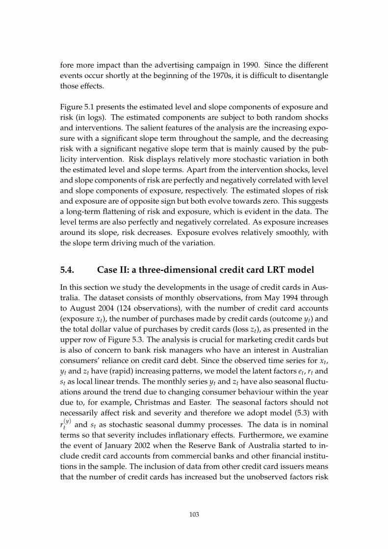
fore more impact than the advertising campaign in 1990. Since the different
events occur shortly at the beginning of the 1970s, it is difficult to disentangle
those effects.
Figure 5.1 presents the estimated level and slope components of exposure and
risk (in logs). The estimated components are subject to both random shocks
and interventions. The salient features of the analysis are the increasing expo-
sure with a significant slope term throughout the sample, and the decreasing
risk with a significant negative slope term that is mainly caused by the pub-
licity intervention. Risk displays relatively more stochastic variation in both
the estimated level and slope terms. Apart from the intervention shocks, level
and slope components of risk are perfectly and negatively correlated with level
and slope components of exposure, respectively. The estimated slopes of risk
and exposure are of opposite sign but both evolve towards zero. This suggests
a long-term flattening of risk and exposure, which is evident in the data. The
level terms are also perfectly and negatively correlated. As exposure increases
around its slope, risk decreases. Exposure evolves relatively smoothly, with
the slope term driving much of the variation.
5.4. Case II: a three-dimensional credit card LRT model
In this section we study the developments in the usage of credit cards in Aus-
tralia. The dataset consists of monthly observations, from May 1994 through
to August 2004 (124 observations), with the number of credit card accounts
(exposure xt), the number of purchases made by credit cards (outcome yt) and
the total dollar value of purchases by credit cards (loss zt), as presented in the
upper row of Figure 5.3. The analysis is crucial for marketing credit cards but
is also of concern to bank risk managers who have an interest in Australian
consumers’ reliance on credit card debt. Since the observed time series for xt,
yt and zt have (rapid) increasing patterns, we model the latent factors et, rt and
st as local linear trends. The monthly series yt and zt have also seasonal fluctu-
ations around the trend due to changing consumer behaviour within the year
due to, for example, Christmas and Easter. The seasonal factors should not
necessarily affect risk and severity and therefore we adopt model (5.3) with
r(y)t and st as stochastic seasonal dummy processes. The data is in nominal
terms so that severity includes inflationary effects. Furthermore, we examine
the event of January 2002 when the Reserve Bank of Australia started to in-
clude credit card accounts from commercial banks and other financial institu-
tions in the sample. The inclusion of data from other credit card issuers means
that the number of credit cards has increased but the unobserved factors risk
103

parameter description Case I Case II Case III
×10−3 ×10−5 ×10−4
Σ(ee)η variance trend exposure 0.31 1.33
Σ(rr)η variance trend risk 1.30 8.91
Σ(ss)η variance trend severity 1.18
Σ(er)η covariance trend exposure-risk −0.640
Σ(ee)ζ variance slope exposure 0.040 0.0261 0.27
Σ(rr)ζ variance slope risk 0.130 0.1590 20.0
Σ(ss)ζ variance slope severity 0.0014
Σ(er)ζ covariance slope exposure-risk −0.070 −0.0371
Σ(es)ζ covariance slope exposure-severity −0.0058
Σ(rs)ζ covariance slope risk-severity 0.0056
Σ(yy)ω variance seasonal outcome 220
Σ(zz)ω variance seasonal loss 181
Σ(yz)ω covariance seasonal outcome-loss 194
Σ(xx)u variance disturbance exposure 0.16 0.31 9.70
Σ(yy)u variance disturbance outcome 4.21 1.07 0.47
Σ(zz)u variance disturbance loss 4.13
intervention description Case I Case II Case III
D(r)t (1970; 2) “war on 1034” −0.079∗∗∗
D(r)t (1971; 1) seat belt law introduction −0.108∗∗∗
D(e)t (1980; 1) data collection change −0.086∗∗
D(r)t (1990; 1) advertising initiative −0.376∗∗∗
D(e)t (1992; 1) data collection change −0.066∗∗∗
D(x)t (2002.1; 1) data collection change 0.062∗∗∗
D(y)t (2002.1; 1) data collection change 0.066∗∗
D(s)t (2002.1; 1) data collection change 0.083∗∗∗
D(e)t (1991; 1) free travel pass introduction −0.180∗∗
D(r)t (2000; 1) start of law moped on main road −0.310∗∗∗
Figure 5.2. Parameter estimates for disturbance (co)variances and interventions. In caseof interventions, ∗∗ and ∗∗∗ indicate significance at 90% and 95% levels, respectively. Thelast three columns are for the three models described in the sections for Case I, II and III.
104

and severity may also change since the new issuers in the sample of credit card
users may represent customers with different spending patterns. The change
in the composition of the sample in January 2002 is permanent and therefore
level interventions for this month are appropriate and are included for the la-
tent trend factors et, rt and st.
1994 1999 2004
8000
10000
12000
1994 1999 2004
50000
100000
1994 1999 2004
5000
10000
15000
1994 1999 2004
9.0
9.2
9.4
1994 1999 2004
1.5
2.0
1994 1999 2004
-2.3
-2.2
-2.1
-2.0
1994 1999 2004
0.0000
0.0025
0.0050
0.0075
1994 1999 2004
0.00
0.01
0.02
1994 1999 2004
0.002
0.003
0.004
Figure 5.3. Monthly time series related to credit cards data from Australia (row 1): num-ber of cards (xt), number of purchases (yt) and their value (zt). Smooth estimates of ex-posure (column 1), risk (column 2) and severity (column 3) factors modelled as stochas-tic trends (row 2) with stochastic slopes (row 3). Intervention estimates are added to thetrends.
The parameter estimates are given in Table 5.2. The variance matrices for trend
and observation noises are taken as diagonal. This is strongly supported by
the fact that maximum likelihood estimation produces almost equal likelihood
values for models with and without this restriction. The estimated variances
of the seasonal disturbances are relatively large compared to the observation
noise. Further, the estimate for the seasonal covariance Σ(yz)ω implies a high
correlation and it may therefore be sufficient to consider model (5.2) with the
inclusion of a seasonal component for rt only. The estimated trends presented
in Figure 5.3 are smooth and their slopes are varying over time. The log-risk
growth is decreasing from 1999 onwards while severity growth is more con-
stant over time. Exposure growth is hump-shaped. The three intervention
estimates are highly significant and are added to the estimated trends in Fig-
ure 5.3 despite that they are part of the observation equations. Although the
risk factor is significantly affected by the intervention for the change in sur-
vey composition, the severity of credit card purchases increased the most. It
105

can therefore be concluded that the new account holders in the survey from
January 2002 onwards are making more expensive purchases with their credit
cards. The new customers have had a smaller effect on the risk (intensity) of
making a purchase.
5.5. Case III: a multiple exposure LRT model
The yearly number of persons killed and seriously injured (KSI) in collisions
between mopeds and bicycles in the Netherlands is closely watched since they
involve mostly young persons. Further, mopeds and bicycles are widely and
intensively used in the Netherlands. An official study was carried out to in-
vestigate the risk of this category of KSI accidents. For this purpose, a dataset
has been constructed with two exposure variables (I = 2) and one outcome
variable (J = 1). The two exposure variables consist of the numbers of kilo-
metres driven by mopeds and by bicycles. The outcome variable is the yearly
number of accidents where the primary collision partners are one moped user
and one bicycle user, and where the victims are either killed or hospitalised.
The yearly observations ranges from 1985 to 2003. Given the short sample, the
model used was parsimonious to preserve a sufficient number of degrees of
freedom.
The three time series are presented in the upper panels of Figure 5.4. For the
two exposure series, the 95% confidence intervals are also presented. These
are based on the published survey error variances. The number of kilometres
driven by bicycles are subject to stepwise increases in the late 1980s and in 1994
while those by mopeds show a gradual decrease over the years. The increase
in 1994 for the bicycle kilometres driven may be explained by the extension
of the sample with persons under 12 years of age. The decrease of the 95%
confidence intervals for the two exposure series from 1994 onwards is due to
the increase of the survey sample size by a factor of two. The yearly num-
ber of accidents show stepwise decreases in 1991 and in 2000. It is anticipated
that the decrease in 1991 coincides with the introduction of a free travelpass
for students (typically between 17 and 21 years of age). The travelpass gave
free access to the national and local public transport systems (mainly buses
and trains). The usage of the free travelpass became more and more restricted
over the years from 1995 onwards. This may partly explain the slow increase
of KSI accidents in the late 1990s. It is reasonable to argue that the decrease in
2000 may have been caused in part by the introduction of a law that moved
all mopeds from the special bicycle roads (or tracks) to the main roads in use
by other motorized vehicles (motors, cars, trucks). This law only applies to
situations where special bicycle roads or tracks exist and where the traffic con-
106
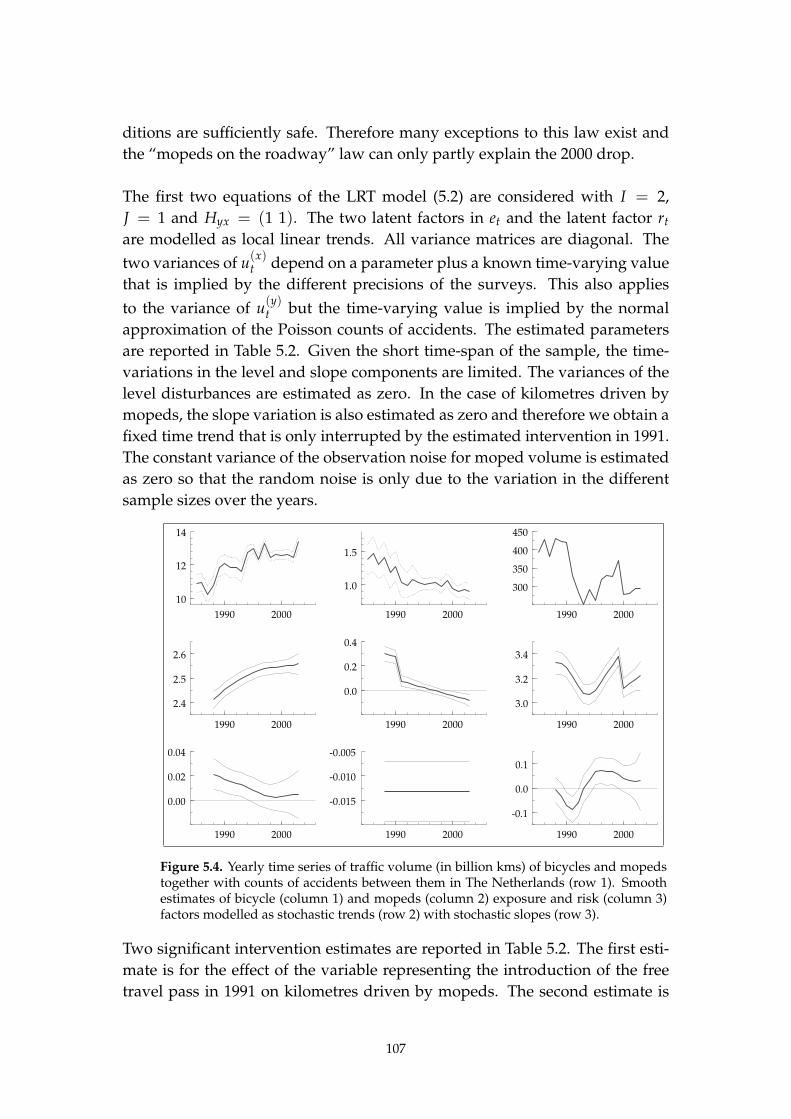
ditions are sufficiently safe. Therefore many exceptions to this law exist and
the “mopeds on the roadway” law can only partly explain the 2000 drop.
The first two equations of the LRT model (5.2) are considered with I = 2,
J = 1 and Hyx = (1 1). The two latent factors in et and the latent factor rt
are modelled as local linear trends. All variance matrices are diagonal. The
two variances of u(x)t depend on a parameter plus a known time-varying value
that is implied by the different precisions of the surveys. This also applies
to the variance of u(y)t but the time-varying value is implied by the normal
approximation of the Poisson counts of accidents. The estimated parameters
are reported in Table 5.2. Given the short time-span of the sample, the time-
variations in the level and slope components are limited. The variances of the
level disturbances are estimated as zero. In the case of kilometres driven by
mopeds, the slope variation is also estimated as zero and therefore we obtain a
fixed time trend that is only interrupted by the estimated intervention in 1991.
The constant variance of the observation noise for moped volume is estimated
as zero so that the random noise is only due to the variation in the different
sample sizes over the years.
1990 2000
10
12
14
1990 2000
1.0
1.5
1990 2000
300
350
400
450
1990 2000
2.4
2.5
2.6
1990 2000
0.0
0.2
0.4
1990 2000
3.0
3.2
3.4
1990 2000
0.00
0.02
0.04
1990 2000
-0.015
-0.010
-0.005
1990 2000
-0.1
0.0
0.1
Figure 5.4. Yearly time series of traffic volume (in billion kms) of bicycles and mopedstogether with counts of accidents between them in The Netherlands (row 1). Smoothestimates of bicycle (column 1) and mopeds (column 2) exposure and risk (column 3)factors modelled as stochastic trends (row 2) with stochastic slopes (row 3).
Two significant intervention estimates are reported in Table 5.2. The first esti-
mate is for the effect of the variable representing the introduction of the free
travel pass in 1991 on kilometres driven by mopeds. The second estimate is
107

for the variable representing the effect of the law of “mopeds on the roadway”
on risk. The extension of the sample for bicycle volume with children under
12 years of age did not affect the analysis. We also have experimented with
other possible interventions but their inclusion had little or no impact on the
value of the likelihood function. The estimated smooth trends for exposure
and risk are displayed in Figure 5.4. Risk is decreasing until the early 1990s,
but has been increasing since 1993. The estimated slope pattern for risk may
be explained by the popularity of light mopeds for which it is not obligatory
to wear a crash helmet. It is evident that accidents are likely to be more severe
when the concerned moped drivers do not wear helmets. This may explain the
increasing trend in KSI accidents.
5.6. Conclusions
In this paper we propose a latent risk time series model for measuring event
risk. The multivariate modelling framework includes latent dynamic factors
for exposure, risk and severity. The multivariate nature of the model means
that common factors can be identified through the correlation structure of la-
tent dynamic processes. The magnitude and sign of correlations may provide
interesting interpretations for researchers. The stochastic trend and seasonal
factors are time-varying by nature and arbitrary re-calibrations of model pa-
rameters are not needed. This is an advantage inherent in the unobserved
components time series modelling approach.
The application to credit cards data showed that stochastic variation is im-
portant in measuring the risk and severity of credit card purchases. For the
car insurance data, stochastic variation seems less important. It appears that
structural breaks explain most of the changes in risk and exposure over the
past 50 years. The illustration of accidents between mopeds and bicycles has
shown that the model can also include multiple categories of exposure varia-
bles. When more data is available, more detailed categories of exposure, risk
and severity can be considered. For example, different risk factors can be in-
cluded for males/females, different age groups and different regions. Future
research is directed towards extending the modelling framework further for
handling multiple categories or panel (longitudinal) structures in data.
108

6. Multivariate nonlinear time series modelling
of exposure and risk in road safety research27
In this paper we consider a multivariate nonlinear time series model for the analysis of traffic
volumes and road casualties inside and outside urban areas. The model consists of dynamic
latent (unobserved) factors for exposure and risk that are related in a nonlinear way. The
multivariate dimension of the model is due to its inclusion of multiple time series for inside
and outside urban areas. The analysis is based on the extended Kalman filter. Approximate
maximum likelihood methods are utilised for the estimation of unknown parameters. The
latent factors are estimated by extended smoothing methods. We present a case study of yearly
time series of numbers of fatal accidents (inside and outside urban areas) and numbers of
driven kilometers by motor vehicles in the Netherlands between 1961 and 2000. The analysis
accounts for missing entries in the disaggregated numbers of driven kilometres although the
aggregated numbers are observed throughout. It is concluded that the salient features of the
observed time series are captured by the model in a satisfactory way.
6.1. Introduction
This paper considers a multivariate nonlinear time series model for the analy-
sis of traffic volume and road accident data. The model is based on the class
of multivariate unobserved components time series models and is modified to
allow for nonlinear relationships between components. The analysis relies on
disaggregated and aggregated data and can account for missing entries in the
data set. Missing observations are quite usual in road safety analysis where
disaggregated data are not available throughout the sample period but data at
the aggregated level are available for a longer period. The nonlinear nature of
the model arises from the fact that locally the expected number of fatal acci-
dents for a year equals risk times exposure estimates for that year. This multi-
plicative relationship can be made additive by taking logarithms in the usual
way. However since the analysis is based on aggregated and disaggregated
data, summing constraints need to be considered as well. This mixture of mul-
tiplicative and additive relations in the model calls for a nonlinear analysis.
Furthermore, the analysis is for a vector of time series and the model consists
of multiple latent variables. Therefore, we adopt multivariate nonlinear state
space methods for the analysis of road accidents.
The empirical motivation is to analyse the development of road safety inside
and outside urban areas in the Netherlands between 1961 and 2000. The ex-
27Co-authored with Jacques Commandeur, SWOV Institute for Road Safety Research, Lei-dschendam, Netherlands, and Siem Jan Koopman and Kees van Montfort, Department ofEconometrics, Vrije Universiteit Amsterdam, Netherlands.
109

pected annual number of fatal accidents is defined by a risk factor times ex-
posure. Risk and exposure are simultaneously treated as latent or unobserved
components. The expected number of vehicle kilometres driven (traffic vol-
ume) is set equal to the latent exposure component. The observed traffic vol-
ume and the observed number of fatal accidents are available for inside and
outside urban areas in the Netherlands. However, for some periods only the
total number of vehicle kilometres driven (the sum of numbers for inside and
outside urban areas) is available. For these periods, the expected total number
of vehicle kilometres is set equal to the sum of the latent exposure components
for inside and outside urban areas.
Since the seminal paper of Smeed (1949), time ordered accident data are anal-
ysed in many studies in road safety. In Smeed (1949) it is argued that the
annual number of fatalities per registered motor vehicle can be explained by
means of the motorisation, measured by the number of registered motor ve-
hicles per capita. The availability of more detailed time series data has led
to advanced and interesting statistical studies on road safety. An example is
the introduction of the use of traffic volume data. Traffic volume (e.g. ve-
hicle kilometres driven, sometimes travel kilometres) is currently assumed to
be one of the most important factors available for the explanation of accident
counts. Appel (1982) found an exponentially decaying risk when he decom-
posed the (expected) number of accidents in a risk component (accidents per
kilometres driven) and exposure (kilometres driven). Similar approaches have
been adopted by Broughton (1991) and Oppe (1989, 1991b). These models are
univariate (one dependent variable) and some consist of just one explanatory
variable measuring traffic volume. Time-dependencies in the error structure
are ignored and estimation is based on classical methods.
Various time series analysis techniques, on the other hand, do take time-depen-
dencies in the error structure into account. For example, autoregressive inte-
grated moving average (ARIMA) techniques with explanatory variables (ARI-
MAX) as developed by Box and Jenkins (1976) are used in the DRAG (De-
mand for Road use, Accidents and their Gravity) analyses of Gaudry (1984)
and Gaudry and Lassarre (2000). A DRAG analysis consists of three stages:
first the traffic volume is modelled, next the accidents using the estimated traf-
fic volume, and then the number of victims per accident (severity). Such a
DRAG analysis is focussed on explaining the underlying factors of road safety
while earlier studies were more focussed on forecasting. The DRAG approach
allows for a non-linear transformation of the data by means of Box-Cox trans-
forms. The time series structure however is linear. The model in this paper
110
disentangles exposure and risk by unobserved components that are estimated
simultaneously rather than estimated by separate stages.
An alternative method to analysing road safety data was proposed by Harvey
and Durbin (1986) and is based on a structural time series model with inter-
ventions. This approach has been applied in road safety analysis by a number
of authors. Ernst and Bruning (1990), for example, used a structural time series
model to assess the effect of a German seat belt law while Lassarre (2001) ap-
plied structural time series models to compare the road safety developments
in a number of countries. The method of Harvey and Durbin (1986) can also
be extended to the simultaneous modelling of traffic volume, road safety and
severity, see Bijleveld et al. (2008). In these approaches linear Gaussian time se-
ries techniques such as the Kalman filter are used for estimation, analysis and
forecasting. In the present paper we need to adopt a nonlinear equivalent of a
structural time series model. Linear estimation techniques cannot be used as a
result and therefore we rely on extended (nonlinear) Kalman filter techniques.
Related approaches based on counts and with latent factors were discussed by
Johansson (1996).
In road safety analysis, the use of disaggregated data is useful when the sepa-
rate series can be modelled more effectively than the original aggregated time
series. For instance, the composition of transport modes inside urban areas is
usually different from that outside urban areas. Therefore, traffic volume and
safety are different in these two parts of the traffic system. The present paper
implements a model-based simultaneous treatment of traffic volume and fa-
tal accidents for inside and outside urban areas. An important feature of the
method is that it can handle the temporal unavailability of traffic volume data
at the disaggregated level, while still providing estimates of the disaggregated
exposure and risk for the full sample.
The paper is organised as follows. Section 6.2 presents the data used in the
application part of the paper. The relation between observed and unobserved
factors within a multivariate nonlinear time series model is described in detail
in Section 6.3, by first introducing the model and then providing a state space
formulation of the model. A description of the estimation methods is given
in Section 6.4. The main empirical results are presented in Section 6.5, and
in Section 6.6 implications for road safety research are discussed. Section 6.7
concludes.
111

1960 1970 1980 1990 2000
20
40
60
80
100
120
1960 1970 1980 1990 2000
200 400 600 80010001200140016001800
Figure 6.1. Traffic volume in billions of motor vehicle kilometres (left panel) and thenumber of fatal accidents (right panel) for inside urban areas (solid line) and outside ur-ban areas (dashed line). The total traffic volume in the left panel is marked by a dashedline over the whole period. The vertical lines inside the graphs mark the period inwhich disaggregated traffic volume data are available. This data-set will be modelled.
6.2. Data description
In the empirical study we analyse annual road traffic statistics from the Neth-
erlands consisting of numbers of fatal accidents and traffic volume, defined as
kilometres driven by motor vehicles, in the period 1961 up to and including
2000, both separated into inside and outside urban areas. This yields y1t as the
traffic volume inside urban areas, y2t as the traffic volume outside urban areas,
y3t as the total traffic volume, x1t as the number of fatal accidents inside urban
areas and x2t as the number of fatal accidents outside urban areas where time
index t = 1, . . . , n represents the index range for the years from 1961 up to and
including 2000. The total number of time points is therefore n = 40. All data
were obtained from the Dutch Ministry of Transport and Statistics Netherlands
while the accident information originated from police records.
The five time series are presented in Figure 6.1 with two displays. The left
hand display shows the development of the motor vehicle kilometres in the
Netherlands. Disaggregated figures of traffic volume y1t and y2t are missing
for the periods 1961 up to and including 1983 and 1997 up to and including
2000. For these years only the total traffic volume y3t is available. Only modest
deviations from an almost linear increase can be noticed from the traffic vol-
ume figures. These deviations are potentially caused by economic factors. The
right hand display in Figure 6.1 shows the development of the number of fa-
tal accidents in the Netherlands, both for inside and outside urban areas. The
total number of fatal accidents increased until the early 1970s. Since then the
trend has reversed, although the rate of decrease seems to slow down near the
end of the series.
112

1960 1970 1980 1990 2000
60
80
100
120
140
160
1960 1970 1980 1990 2000
51
53
55
57
59
Figure 6.2. Traffic intensity index (left panel) and total length in kilometers of mainroads outside urban areas (right panel). The vertical lines inside the graphs mark theperiod in which disaggregated traffic volume data are available. This data-set is usedfor external model validation.
The results of the empirical analysis in Section 6.5 will be validated against an
alternative estimate of the traffic volume outside urban areas. This estimate is
composed of indexed figures on traffic intensity on main roads multiplied by
the length of the road system outside urban areas as obtained from a survey of
municipalities, which is not available for all time points. The data for these two
time series are presented in Figure 6.2. The data of the last years are considered
to be inconsistent due to changes in registration. The product of the latter two
series should be roughly equal to the development of motor vehicle kilometres
outside urban areas when it is assumed that the development of the traffic
intensity outside urban areas is approximately proportional to the intensity on
the main roads.
6.3. The multivariate nonlinear time series model
6.3.1. Specification of model and assumptions
The multivariate nonlinear time series model is based on two unobserved com-
ponents: a component for exposure (traffic volume) and a component for risk.
Each component is bivariate to disentangle the effects for inside and outside
urban areas. The statistical specification of the components is based on linear
dynamic processes. The observed time series of fatal accidents and driven mo-
tor vehicle kilometres depend on these factors. In particular, (i) the expected
number of fatal accidents is the product of risk and exposure, (ii) the expected
number of driven motor vehicle kilometres is proportional to the unobserved
factor exposure and (iii) the expected total number of driven motor vehicle
kilometres is proportional to the sum of the unobserved factors of exposure
inside and outside urban areas. The dynamic specifications of the unobserved
components are based on flexible time-varying trend functions. The level of
113

1960 1970 1980 1990 2000
20
40
60
80
100
120
1960 1970 1980 1990 2000
2
3
4
5
Figure 6.3. The total number of fatal accidents per billion vehicle kilometres(left panel) and in logs (right panel). The vertical lines inside the graphsmark the period in which disaggregated traffic volume data are available.
smoothness of these trends can be estimated. Note that it will be found that
the unobserved exposure components will effectively increase with time while
the unobserved risk components steadily decrease with time. As a result, be-
cause the increase in exposure coincides with a decrease in risk, the relation
between exposure and the number of accidents flattens off, as it often does
when nonlinear relations are assumed (Hauer, 1995). In addition, the general
risk is likely to have decreased. It remains a question whether these effects will
ever be distinguishable, as relations like proposed in (Hauer, 1995) are likely
to have changed as well over the 40 year period considered in this study. This
has not been attempted in this study.
Disaggregated time series data for inside and outside urban areas are available
for fatal accidents and driven kilometres although for the latter series the data
are not available for the full sample. However the yearly series of total number
of driven kilometres is available for the full sample. The five time series (par-
tially consisting of missing values) are modelled simultaneously. A log-linear
model can be considered to treat the multiplicative dependency (product of
risk and exposure) but it cannot at the same time handle the sum restrictions
for the missing disaggregated data. For this reason we need to adopt a mul-
tivariate and partially nonlinear time series model. Figure 6.1 confirms that
the number of driven kilometers are trending linearly throughout. Another
nonlinear aspect of the model is introduced by the assumption of an exponen-
tial decay over time of risk factors. Figure 6.3 displays the number of fatal
accidents per billion vehicle kilometres (in levels and logs); this is a rough in-
dication of risk. It shows that risk may decay exponentially over time and it
may therefore be reasonable to assume a smooth linear trend function for log-
risk. This exponential trend specification introduces a further nonlinear aspect
in the model. Possible breaks in trends can be accounted for by including in-
tervention regression effects in the model.
114

6.3.2. Unobserved stochastic local linear trend factors
The deterministic trend specifications for exposure and in particular log-risk
are too rigid in practice because trends will not be constant over time in a
long period of forty years. A time-varying trend is more flexible. A possible
stochastic specification for a time-varying trend µt is the local linear trend with
increment or slope term βt and given by
µt+1 = µt + βt + ηt, βt+1 = βt + ζt, t = 1, . . . , n, (6.1)
where the disturbances ηt and ζt are normally distributed with mean zero and
variances σ2η and σ2
ζ , respectively. The disturbances ηt and ζs are mutually and
serially independent of each other at all time points t, s = 1, . . . , n. The initial
values of µ1 and β1 can be regarded as realisations from a diffuse distribution
or as fixed unknown coefficients, see the discussion in Durbin and Koopman
(2001). The special case of σ2η = σ2
ζ = 0 reduces (6.1) to βt+1 = βt = β1 and
µt+1 = µ1 + β1 + . . . + βt = µ1 + β1 · t for t = 1, . . . , n. This is the deterministic
linear trend. In a similar way we can show that for the case of σ2η > 0 and σ2
ζ =
0, we obtain the random walk plus fixed drift ∆µt+1 = β1 + ηt for t = 1, . . . , n.
Further, it can be established that a smooth trend specification can be obtained
by σ2η = 0 and σ2
ζ > 0, see also Harvey (1989) or Commandeur and Koopman
(2007).
The unobserved exposure factors for inside and outside urban areas are indi-
cated by µ1t and µ2t, respectively. The log-risk factors for inside and outside
urban areas are indicated by δ1t and δ2t, respectively. Given the discussion
in the previous section and to gain flexibility in modelling, we consider local
linear trend specifications for the unobserved factors, that is
µit ∼ LLT, δit ∼ LLT, i = 1, 2, t = 1, . . . , n,
where LLT refers to the trend specification (6.1). The disturbance sequences
driving the unobserved factors are mutually independent of each other except
those within the pairs of (µ1t, µ2t) and (δ1t, δ2t). In other words, correlation
between log-risk factors inside and outside urban areas can be estimated. This
also applies to exposure factors.
6.3.3. Observation equation
The dynamic mutual dependencies of the five observed time series are speci-
fied solely through the four unobserved and independent factors. This leads to
a relatively simple model specification for the observed time series. Given the
discussion of the model in Section 6.3.1, the model equations for the observed
115

traffic volume for inside and outside urban areas are given by
yit = µit + εit, εit ∼ WN, i = 1, 2, t = 1, . . . , n, (6.2)
where WN refers to a Gaussian white noise sequence. The disturbances εit
have mean zero and variance σ2ε,i for i = 1, 2. Further, they are mutually inde-
pendent of all other disturbances in the model. The variances σ2ε,1 and σ2
ε,2 need
to be estimated. The total traffic volume is modelled by the relation
y3t = y1t + y2t = µ1t + µ2t + ε1t + ε2t. (6.3)
These observation equations are linear and can be regarded as a special trivari-
ate common trends model with two independent stochastic trends. It should
be noted that when no observations are available for y1t and y2t, the distur-
bances ε1t and ε2t cannot be identified separately. The sum ε1t + ε2t can be
identified when only y3t is observed. Therefore, in this case we take ε1t + ε2t
as a Gaussian white noise sequence with mean zero and variance σ2ε,1 + σ2
ε,2.
The statistical model specification for the number of fatal accidents in and out-
side urban areas is given by
g(µit, δit) = µit · exp(δit), (6.4)
which implies an exponential trend for the log-risk factor that is proportional
to exposure. The Gaussian disturbances ξit have mean zero and a non-negative
variance, for i = 1, 2. They are also mutually independent of all other distur-
bances. The counts of fatal accidents are approximated by a normal distribu-
tion, as the counts vary within the wide interval of 250 and 1750. We account
for possible overdispersion by setting the variance of the disturbances ξit equal
to xit(1 + σ2ξ,i) where we regard the fatal accidents xit as a proxy for the mean
of xit.
6.3.4. Nonlinear state space model formulation
The general state space model with a (possible) nonlinear observation equation
is given by
(
yt
xt
)
= Z(αt)+ Gut, αt+1 = Tαt + Hut, ut ∼ WN, t = 1, . . . , n,
(6.5)
116

where αt is the state vector and ut is the disturbance vector with mean zero
and variance matrix V. The system matrices G, T and H together with the
function Z(·) are fixed and known although they may partially depend on
a parameter vector of fixed unknown coefficients. The initial state vector is
taken as a realisation from a diffuse density but can also be regarded as fixed
unknown coefficients, see Durbin and Koopman (2001, Chapter 6).
The local linear trend models for exposure and log-risk, inside and outside ur-
ban areas, can be simultaneously put in state space form by placing the trends
µit and δit with their associating slope terms, for i = 1, 2, in the state vector αt.
The disturbance terms are put in ut. We obtain,
αt =(µ1t, βµ1t, µ2t, β
µ2t, δ1t, βδ
1t, δ2t, βδ2t)
′,
ut =(ηµ1t, ζ
µ1t, ε1t, η
µ2t, ζ
µ2t, ε2t, ηδ
1t, ζδ1t, ξ1t, ηδ
2t, ζδ2t, ξ2t, )
′,
where xµ indicates the association of variable x with exposure µ and xδ with
log-risk factor δ for x = β, η, ζ. The stochastic processes for the four trend
functions are implied by the system matrices given by
T = I4 ⊗[
1 1
0 1
]
, H = I4 ⊗[
1 0 0
0 1 0
]
,
where I4 is the 4 × 4 identity matrix and ⊗ is the Kronecker matrix product.
The multivariate observation equation for traffic volume is linear. In terms of
the observation vector yt = (y1t, y2t, y3t)′ and the state vector αt it follows from
(6.2) and (6.3) that
yt =
1 0 0 0
0 1 0 0
1 1 0 0
⊗
(
1 0)
αt +
1 0 0 0
0 1 0 0
1 1 0 0
⊗
(
0 0 1)
ut. (6.6)
This observation equation is rank deficient due to its inclusion of identity (6.3).
However, during the estimation process, the equation for y3t is only considered
when y1t and y2t are missing and y3t is not considered when y1t and y2t are not
missing. The estimation method does this implicitly through its treatment of
missing values.
The observation equation for the number of fatal accidents, inside and outside
urban areas, can also be formulated in terms of the state vector αt but it requires
a nonlinear specification. Define xt = (x1t, x2t)′ and consider (6.5) where Z(αt)
117

and G are chosen such that
xt =
(
µ1t · exp δ1t
µ2t · exp δ2t
)
+
[
0 0 1 0
0 0 0 1
]
⊗(
0 0 1)
ut, (6.7)
with(
µ1t
µ2t
)
=
[
1 0 0 0
0 1 0 0
]
⊗(
1 0)
αt,
(
δ1t
δ2t
)
=
[
0 0 1 0
0 0 0 1
]
⊗(
1 0)
αt.
This completes the state space formulation of the multivariate nonlinear model
that is the basis of the empirical study discussed in Section 6.5.
6.4. Estimation of parameters and latent factors
The variances of the disturbances in vector ut of the state space model in the
previous section are treated as unknown parameters. They will be estimated
by the method of maximum likelihood. For a fully linear model, the Gaussian
log-likelihood function is evaluated by the Kalman filter and numerically max-
imised with respect to the unknown parameters, see Harvey (1989) and Durbin
and Koopman (2001). Consider a state space model with a linear Gaussian ob-
servation equation
(
yt
xt
)
= ct + Zt · αt + Gut, (6.8)
where ct is a known vector and Zt is a known matrix. Both can be time-varying
and may depend on past observations. It is noticed that the linear Gaussian
model (6.8) is equivalent to (6.5) with Z(αt) = ct + Zt · αt. Further, we assume
that the disturbances ut are normally distributed.
The Kalman filter recursively evaluates the estimator of the state vector con-
ditional on past observations Yt−1 = {y1, x1, . . . , yt−1, xt−1}. The conditional
estimator of the state vector is denoted by at|t−1 = E(αt|Yt−1) and its condi-
tional variance matrix Pt|t−1 = var(αt|Yt−1). The Kalman filter is given by the
118
set of vector and matrix equations
vt =
(
yt
xt
)
− ct − Ztat|t−1, Ft = ZtPt|t−1Z′t + GG′,
Kt = (TPt|t−1Z′t + HG′)F−1
t ,
at+1|t = Tat|t−1 + Ktvt, Pt+1|t = TPt|t−1T′ − KtF−1t K′
t + HH′,
(6.9)
for t = 1, . . . , n and where a1|0 and P1|0 are the unconditional mean and var-
iance of the initial state vector, respectively. When an initial state element is
taken as a realisation from a diffuse density, we can take its mean as zero and
its variance as a very large value. Exact treatments of diffuse initialisations
are discussed in Durbin and Koopman (2001). The vector vt is the one-step
ahead prediction error with variance matrix Ft. The optimal weighting for fil-
tering is determined by the Kalman gain matrix Kt. The joint density of the
observations can be expressed as a product of predictive densities via the pre-
diction error decomposition. As a result, the log-likelihood function can be
constructed via the Kalman filter and is given by
ℓ = −n
2log 2π − 1
2
n
∑t=1
log |Ft| −1
2
n
∑t=1
v′tF−1t vt. (6.10)
With diffuse state elements, the log-likelihood function requires some modifi-
cations. For a linear Gaussian state space model, the log-likelihood function ℓ
is exact.
When a value for a particular element of vector (y′t, x′t)′ is not available, it is
treated as a missing value. The Kalman filter can handle missing values in
a straightforward way. Effectively, it measurement is removed. An alterna-
tive approach is to assume its resulting variance tending to infinity. A direct
consequence of a missing entry is that the associated element of the innova-
tion vector vt cannot be computed and is unknown. Assume that all entries
in (y′t, x′t)′ are missing, we can treat vt as unknown by taking vt = 0 and, its
variance matrix, Ft → ∞I such that F−1t → 0 and Kt → 0. It follows that the
state update equations become
at+1|t = Tat|t−1, Pt+1|t = TPt|t−1T′ + HH′.
These computations are repeated for when a number of (consecutive) obser-
vations are missing. This solution also serves as the basis for out-of-sample
forecasting (future values are missing) or back-casting (past values are miss-
119
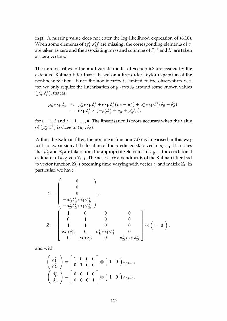
ing). A missing value does not enter the log-likelihood expression of (6.10).
When some elements of (y′t, x′t)′ are missing, the corresponding elements of vt
are taken as zero and the associating rows and columns of F−1t and Kt are taken
as zero vectors.
The nonlinearities in the multivariate model of Section 6.3 are treated by the
extended Kalman filter that is based on a first-order Taylor expansion of the
nonlinear relation. Since the nonlinearity is limited to the observation vec-
tor, we only require the linearisation of µit exp δit around some known values
(µ∗it, δ∗it), that is
µit exp δit ≈ µ∗it exp δ∗it + exp δ∗it(µit − µ∗
it) + µ∗it exp δ∗it(δit − δ∗it)
= exp δ∗it × (−µ∗itδ
∗it + µit + µ∗
itδit),
for i = 1, 2 and t = 1, . . . , n. The linearisation is more accurate when the value
of (µ∗it, δ∗it) is close to (µit, δit).
Within the Kalman filter, the nonlinear function Z(·) is linearised in this way
with an expansion at the location of the predicted state vector at|t−1. It implies
that µ∗it and δ∗it are taken from the appropriate elements in at|t−1, the conditional
estimator of αt given Yt−1. The necessary amendments of the Kalman filter lead
to vector function Z(·) becoming time-varying with vector ct and matrix Zt. In
particular, we have
ct =
0
0
0
−µ∗1tδ
∗1t exp δ∗1t
−µ∗2tδ
∗2t exp δ∗2t
,
Zt =
1 0 0 0
0 1 0 0
1 1 0 0
exp δ∗1t 0 µ∗1t exp δ∗1t 0
0 exp δ∗2t 0 µ∗2t exp δ∗2t
⊗(
1 0)
,
and with(
µ∗1t
µ∗2t
)
=
[
1 0 0 0
0 1 0 0
]
⊗(
1 0)
at|t−1,
(
δ∗1t
δ∗2t
)
=
[
0 0 1 0
0 0 0 1
]
⊗(
1 0)
at|t−1.
120

The extended Kalman filter approximates the nonlinear features of the model.
The prediction error is therefore not evaluated exactly and the log-likelihood
function (6.10) is an approximation.
The smoothed estimate of a latent factor is the conditional mean given all avail-
able observations in the sample. The smoothed estimate of the state vector is
denoted by αt = E(αt|Yn) with its variance matrix Vt = var(αt|Yn). Once the
Kalman filter is carried out, the smoothed estimates can be computed via the
backward recursions
rt−1 = Z′tF
−1t vt + L′
trt−1, Nt−1 = Z′tF
−1t Zt + L′
tNt−1Lt,
αt = at|t−1 + Pt|t−1rt−1, Vt = Pt|t−1 − Pt|t−1Nt−1Pt|t−1,(6.11)
where Lt = T −KtZt and with initialisations rn = 0 and Nn = 0. The algorithm
is a variation of the fixed interval smoothing method of Anderson and Moore
(1979) and is developed by de Jong (1989) and Kohn and Ansley (1989). The
smoothing recursions apply to the linear Gaussian state space model. How-
ever, since we have explicitly used a time-varying Zt, the computations can
also be carried out in conjunction with the extended Kalman filter. We note
that smoothing requires the storage of all Kalman filter quantities, including
the time-varying values of ct and Zt, for t = 1, . . . , n.
6.5. Empirical results: estimation and model selection
We consider the five time series described in Section 6.2 for the years 1961–
2000. The disaggregated time series of traffic volume is only observed for the
sample 1984–1996 and therefore we are dealing with many missing values in
the data set. The traffic volume series yit are modelled by (6.2) while the num-
ber of fatal accidents series xit are modelled by (6.4). Note that i = 1 refers
to outside urban areas and i = 2 refers to inside urban areas. The total traffic
volume y3t is considered when disaggregated data are not available and model
(6.3) applies. The full model consists of two sets (for outside and inside urban
areas) of two unobservable trend functions (for exposure and for log-risk). For
each trend we need to estimate two variances while for each observation equa-
tion we need to estimate an additional variance. The total number of parame-
ter is therefore 12. Finally, in our nonlinear multivariate model of Section 6.3,
the counts of yearly accidents xit are approximated by a normal distribution.
To account for possible overdispersion we have set the disturbance variances
of ξit, for i = 1, 2, equal to (1 + σ2ξ,i)xit. The implication is that matrix G in (6.5)
is effectively time-varying. Note that the prediction of the number of accidents
(see (6.4)) is a function of stochastic processes rather than a function of fixed
121
explanatory variables as is assumed in many classical models. Therefore the
model assumes more dispersion than ξit, for i = 1, 2.
At a closer inspection of the number of fatal accidents series in the right panel
of Figure 6.1, it is clear that trend-breaks occur in the years of 1974 and 1975.
They can (partly) be attributed to the global ‘oil crisis’ in 1974 and the intro-
duction of alcohol legislation in the Netherlands (November 1974). In the next
year, legislation on wearing moped helmets (February 1975) and seat belt legis-
lation (June 1975) were introduced. We therefore have included dummy effects
for trend breaks in 1974 and 1975 in the equations for yearly accidents xit, for
i = 1, 2. These dummy effects are estimated simultaneously with the other
parameters in the model.
6.5.1. Parameter estimation results
Table 6.4 presents the estimates of the parameters in the model including the
variances and dummy effects of trend breaks. The table reports the estimates
together with 95% lower and upper limits of the confidence intervals. The con-
fidence intervals are based on the approximation discussed in Harvey (1989,
§3.4.5 and §3.4.6). Since variance parameters are restricted to be non-negative,
the logged variances are estimated and related confidence intervals are there-
fore asymmetric. We do not report parameters that have been estimated very
closely to zero. These are (i) the variances σ2ξ,i for both i = 1, 2, (ii) the var-
iances of level disturbances ηµit for both i = 1, 2, (iii) the variances of slope
disturbances ζδit for both i = 1, 2 and (iv) the dummy effect for the 1975 trend
break in log-risk for outside urban areas (i = 2).
From these results we learn that overdispersion of counts in the Gaussian ap-
proximation are not significant. This is probably due to additional variance
already by the model. Further, the estimated zero level variances in the expo-
sure components µit, for i = 1, 2, lead to so-called smooth trends for µit. The
estimates of the slope variances in exposure, as reported in Table 6.4, reveal
that the variation in exposure growth is larger for outside (≈ 1.70) than for
inside urban areas (≈ 0.03). These estimates rely on the limited sample period
1984–1996. The time series plots in Figure 6.1 confirm that the traffic volume
inside urban areas is almost constant over these years while the growth of traf-
fic volume outside urban areas has increased more rapidly in the period before
1990 than the period after 1990. Also, traffic volume inside urban areas appear
to be noisier than traffic volume outside urban areas (compare the observation
variances for outside, ≈ 0.08, and inside, ≈ 0.75, in Table 6.4). The slope vari-
ances of the log-risk components are estimated zero. This reduces the log-risk
122

1960 1970 1980 1990 2000
2
3
4
5
1960 1970 1980 1990 2000
20
40
60
80
Figure 6.5. Left panel: Estimated trends of log-risk δit for inside (with fi-nal estimate 2.39, s.e. 0.05) and outside (with final estimate 1.93, s.e. 0.03)urban areas. Right panel: Estimated trends of exposure µit for inside (finalestimate 31.82, s.e. 1.36) and outside (final estimate 94.24, s.e. 1.48) urbanareas. The shaded areas indicate 95% confidence intervals.
trends to random walk processes with fixed growth terms. Both level vari-
ances are estimated to be relatively small since log-risk trends have a much
smaller scale than exposure trends. Although these estimated level variances
are small they deviate from zero significantly.
Parameter Inside urban areas (i = 1) Outside urban areas (i = 2)Est lci uci Est lci uci
Var(ζµit) 0.0312 0.0191 0.0509 1.6999 1.1974 2.4132
Var(ηδit) 0.0012 0.0007 0.0020 0.0012 0.0005 0.0025
Var(εit) 0.7492 0.5177 1.0844 0.0794 0.0183 0.3451Break δit 1974 −0.1822 −0.2850 −0.0794 −0.1705 −0.2567 −0.0842Break δit 1975 −0.1387 −0.2464 −0.0310
Figure 6.4. Estimation results of parameters in equations for inside and outside urbanareas. Estimates are reported, when they significantly deviate from zero, together withlower (lci) and upper (uci) limits of the 95% confidence interval (those for variances areasymmetric).
The estimation results for the dummy effects, as reported in Table 6.4, show
significant breaks in the log-risk trends for the years 1974 and 1975. Only the
break in 1975 for log-risk outside urban areas is not significant. The anticipated
effect of the seat belt law in 1975 may already have its main effect in 1974.
To further disentangle the effects of these events, more detailed accident and
mobility data are required.
6.5.2. Signal extraction: trends for exposure and risk
The left hand panel of Figure 6.5 presents the estimated trends for the log-risk
of inside and outside urban areas. The apparent accelerated decrease in the
trend of the risk for inside urban areas is the result of the interventions in 1974
and 1975 whereas for outside urban areas it is the result of the effect of the in-
tervention in 1974. It appears that the risk outside urban areas decreases more
123
rapidly than the risk inside urban areas. Whether this is due to the increased
implementation of motorways and the separation of long distance traffic from
local traffic requires further investigations.
The right hand panel of Figure 6.5 displays the trends of exposure inside and
outside urban areas. The exposure inside urban areas increases steadily from
the 1960s onwards until it levels off at the end of the 1970s. It starts slowly
increasing again from the 1990s onwards. It may be noted that the stabili-
sation of the exposure inside urban areas in the 1970s takes place before the
period for which disaggregated traffic volume data are available. This shows
that the methodology enables the recognition of such changes before disag-
gregated data are available. In comparison with the trend of exposure inside
urban areas, the confidence margin in the trend of exposure outside urban ar-
eas is small. Moreover, the outside trend is growing more consistently over
the years although some minor temporary fluctuations of trend increases can
be observed. Such fluctuations are detected even at time points where traf-
fic volume data outside urban areas are not available. This can be explained
by the fact that the estimated exposure trends also rely on the observed time
series of number of fatal accidents. Since more fatal accidents occur outside
urban areas, it is apparently more likely that the fluctuations in the number of
accidents affect outside exposure more than inside exposure.
6.5.3. Model fit
This section concentrates on the ability of the multivariate nonlinear model
to fit the time series of motor vehicle kilometres and fatal accidents, inside
and outside urban areas. In Figures 6.6 and 6.7 the model predictions, both
based on only previous observations (one-ahead predictions) and based on
all observations (smoothed predictions) are represented as solid lines, with
approximate 95% confidence intervals represented by shaded areas, and the
observed data are represented as enlarged dots. The confidence intervals are
based on the estimated variances of the disturbances.
The estimated values for the motor vehicle kilometres in Figure 6.6 are equal
to the trends µit for exposure discussed in the previous section. The fit of the
estimated model is quite satisfactory. The estimated number of fatal accidents
in Figure 6.7 is based on the nonlinear function µit exp δit. The effectiveness
of this simple nonlinear relationship is convincing given the good fit of the
estimated number of accidents to the data. Apart from some small differences,
the estimates for inside and outside urban areas show similar patterns. It is
encouraging that the model has identified the sudden increase in the number
of fatal accidents outside urban areas in 1975–1977 – and mainly attributed
124

1960 1970 1980 1990 2000
20
40
60
80
100
120
1960 1970 1980 1990 2000
20
40
60
80
100
120
Figure 6.6. Estimated (solid line) versus observed (dots) motor vehicle kilometres forinside (lower line), outside (middle line) urban areas and total (upper line). Left panel:estimates based on past observations only (prediction). Right panel: estimates basedon all observations (smoothing). Disaggregated traffic volume data are available in theperiod within the vertical lines. The shaded areas are 95% confidence intervals.
1960 1970 1980 1990 2000
200 400 600 800
10001200140016001800
1960 1970 1980 1990 2000
200 400 600 800
10001200140016001800
Figure 6.7. Estimated (solid line) versus observed (dots) number of fatal accidentsfor inside (lower line) and outside (upper line) urban areas. Left panel: estimatesbased on past observations only (prediction). Right panel: estimates based on allobservations (smoothing). Solid lines represent the model estimates and dots arethe observed values. Disaggregated traffic volume data are available in the periodwithin the vertical lines. The shaded areas indicate 95% confidence intervals.
125

1960 1970 1980 1990 2000
-2
-1
0
1
2
3(a)
19831990 1997
-2
-1
0
1
2
3(b)
19831990 1997
-2
-1
0
1
2
3(c)
1960 1970 1980 1990 2000
-2
-1
0
1
2
3(d)
1960 1970 1980 1990 2000
-2
-1
0
1
2
3(e)
Figure 6.8. Standardised prediction residuals for (a) total traffic volume, (b) traffic vol-ume inside urban areas, (c) traffic volume outside urban areas, (d) fatal accidents insideurban areas, (e) fatal accidents outside urban areas. Disaggregated traffic volume dataare available in the period within the vertical lines.
this to an increase in traffic volume (see Figure 6.5) – whereas the number of
accidents inside urban areas almost continues to decrease in this period.
In Figure 6.8 the standardised residuals are displayed. Although these resid-
uals appear not to violate standard univariate tests, it should be noted that
this case is not very standard. The series for traffic volume inside and outside
urban areas are very short, so the power and reliability of – in addition asymp-
totic – tests on such series is limited. Secondly, the series for traffic volume are
interrelated, and as the relatively large deviances in both inside and outside ur-
ban area series are not reflected in the series for the whole of the Netherlands,
one can suspect some correlation here, which is not considered in univariate
tests. Altogether these results should not be considered decisive, rather, the
results can be considered encouraging.
6.5.4. External validation
To further validate the estimates obtained by the model, we consider the esti-
mated trend for the exposure outside urban areas displayed in the right panel
of Figure 6.5. These estimates are also presented as the solid line in Figure 6.9.
Since traffic volume data outside urban areas are only available for the years
1984 up to 1996, the fit between the observed volume data outside urban areas
and the estimated trend can only be evaluated for this 13 year period. How-
ever, as mentioned in Section 6.2, an alternative indicator for exposure outside
126

1960 1970 1980 1990 2000
102030405060708090 Figure 6.9. The fit of traffic volume outside ur-
ban areas: extrapolation and validation of themodel. The fit implied by the multivariate non-linear model is represented by a solid line. Trafficvolume outside urban areas is only available inthe period within vertical lines. The alternativeindicator observations of volume are representedby the dots. The dashed line reflects the linear ex-trapolation of the traffic volume data outside ur-ban areas.
urban areas is available which extends beyond the 13 year period. This alterna-
tive indicator is obtained by multiplying the indexed traffic intensity on main
roads in the Netherlands with the total length of roads outside urban areas.
Since this alternative indicator is measured on a different scale from the motor
vehicle kilometers driven outside urban areas, the values of the latter obser-
vations were regressed on the alternative indicator observations for the years
1984 up to 2000. The predicted values of this simple regression without inter-
cept yield properly re-scaled alternative indicator observations and are plotted
as dots in Figure 6.9. As the figure shows, the estimated trend for exposure out-
side urban areas is quite consistent with the alternative indicator values, even
in the eleven year period from 1973 through 1983 for which no motor vehicle
kilometres driven specific for outside urban areas were available.
Finally, alternative back-casts and forecasts can be produced by the linear ex-
trapolation of traffic volume outside urban areas. These back- and forecasts are
shown in Figure 6.9 as a dashed line. Especially the back-casts of the nonlinear
state space model are clearly superior to a simple extrapolation of the traffic
volume data.
6.6. Implications for road safety research
The current results offer the possibility to interpret the disaggregated develop-
ments of road safety over a much longer period of time than the 13 year period
of 1984 up to and including 1996 for which all disaggregated data are available.
Moreover, it may be that the methodology used in this paper is applicable in
more cases in road safety analysis where where some important exposure fea-
ture is not available in a disaggregation of interest to road safety research, for
instance when a distinction is not yet made in a survey, while already being
available in accident data. In this example a brief period of data availability
was used to extend the disaggregation of traffic volume data to other periods.
In practice however, it is more likely that such a gap in information is filled
using specialist surveys or third party data. Although such data are likely to
127

be only intermittently available in practice, it may be possible that they could
still be used for analysis.
With respect to interpretation of the road safety development in the Nether-
lands, from Figure 6.6 we learn that the development of Dutch traffic volume
has increased since the 1960s. Disaggregating the traffic volume for inside and
outside urban areas shows that the traffic volume inside urban areas contin-
ued to increase until the end of the 1970s. It started to increase again from
the 1990s. On the other hand, the traffic volume outside urban areas kept on
growing more consistently and strongly with the largest acceleration between
about 1983 and 1992. Although the increase of traffic mobility outside urban
areas was limited in the early 1960s, it has increased more dramatically from
the end of the 1960s when comparing it to mobility inside urban areas. It can
therefore be concluded that this development was a dominant factor in the
total traffic volume long before the beginning of the new century. It would
be interesting to further disaggregate the developments, both in terms of road
type and accident type, where the impact of the separation of vulnerable road
users from motorised traffic could be of interest.
6.7. Conclusions
The model-based treatment of exponential and multiplicative relationships be-
tween number of accidents and factors such as exposure and risk has proven
to be effective. A multivariate nonlinear time series model is estimated using
a partially disaggregated data set of traffic volume and number of accidents.
The estimation methods are based on extended versions of the standard multi-
variate Kalman filter and related algorithms. We have shown that a state space
methodology in a multivariate and nonlinear setting with many missing ob-
servations is feasible and that it can lead to interesting empirical results. The
empirical study consists of the analysis of road safety in the Netherlands by
simultaneous consideration of two sections of the total traffic system: inside
and outside urban areas. It is assumed that the development of road safety
inside urban areas is different from the development of road safety outside ur-
ban areas due to differences in road infrastructure and changes in the use of
road transport inside and outside urban areas over the years.
The empirical results show that developments of exposure inside and out-
side urban areas have roughly kept up with each other up to 1980. After this
period, a decline of the growth in exposure inside urban areas occurred and
lasted until approximately 1990. Then exposure inside urban areas started to
increase again. In contrast, the exposure outside urban areas has steadily in-
128
creased since 1980. The model has successfully reconstructed the development
of traffic volume outside urban areas for a long time period. This is confirmed
by considering an alternative estimate of traffic volume outside urban areas,
based on the product of the index of traffic intensity and an estimate of the
total road length, both outside urban areas. The similarity between these alter-
native data-driven estimates and the model estimates is convincing.
Although the empirical results are satisfactory, the methodology of this paper
can be improved further. For example, the model may need to allow for covar-
iances between the disaggregated values. Furthermore, introducing common
components in the model may lead to statistically more significant dynamic
relations between the series. Finally, the consideration of non-Gaussian fea-
tures in the model may enhance the applicability of the current methodology
in cases where small counts are observed.
129

7. The likelihood filter: estimation and testing28
7.1. Introduction
Based on an idea in Bell and Cathey (1993)’s paper on the iterated extended
Kalman filter as a Gauss-Newton method, this paper considers an approach to
filtering and likelihood estimation for state space models where the dependent
variables can be non-Gaussian distributed, not necessarily by an exponential
family distribution. Furthermore, dependence on the state vector is not re-
stricted to location parameters.
In classical linear Gaussian state space models (see e.g., Harvey, 1989) it is
assumed that p × 1 observation vectors yt (t = 1, . . . , n) are generated by the
process:
yt = Zt αt + εt, εt ∼ NID(0, Ht), (7.1)
αt = Tt αt−1 + Rt ηt, ηt ∼ NID(0, Qt), (7.2)
where the error terms εt and ηt are assumed to be zero mean, independent and
identically Gaussian distributed. The unobserved state at time t is represented
by the m × 1 vector αt. Rt is a selection matrix composed of r ≤ m columns of
the identity matrix Im. The variance matrices Qt and Ht are assumed to be non-
singular. In general, the matrices Zt, Tt, Ht and Qt are assumed to be known
or otherwise to depend on an unknown parameter vector ψ.
Following Durbin and Koopman (1997), this paper considers the case where
the linear Gaussian observation model (7.1) is replaced by a general observa-
tion conditional density
p(yt|α1, . . . , αt, y1, . . . , yt−1, ψ) = p(yt|αt, ψ), (7.3)
while the linear state transition equation (7.2) and its Gaussian assumptions
are retained. The likelihood of the state space model is
p(y1, . . . , yn, ψ) = p(y1, ψ)n
∏t=2
p(yt|y1, . . . , yt−1, ψ). (7.4)
28co-authored with Siem Jan Koopman, Department of Econometrics, Vrije UniversiteitAmsterdam, Netherlands.
130
which can be reformulated by conditioning on the state, explicitly expressing
the likelihood in terms of the general observation conditional density p(yt|αt, ψ):
p(y1, . . . , yn, ψ) =n
∏t=1
∫
p(yt|αt, ψ) p(αt|y1, . . . , yt−1, ψ) d αt, (7.5)
where y1, . . . , y0 in p(α1|y1, . . . , y0, ψ) represents, possibly diffuse, prior infor-
mation. Evaluation of (7.5), more specifically the (numerical) evaluation of the
integrals
∫
p(yt|αt, ψ) p(αt|y1, . . . , yt−1, ψ) d αt, (7.6)
can be decisively slow when the dimension of the state m is larger than 1 as
it requires the evaluation of multidimensional integrals, in particular, when
these integrals cannot be evaluated analytically. Durbin and Koopman (1997)
and others address the evaluation of such integrals by means of Monte Carlo
techniques. This paper however considers the use of an analytical evalua-
tion of such integrals based on Laplace approximations, as applied by e.g.
Wolfinger (1993); Vonesh (1996); Huber, Ronchetti, and Victoria-Feser (2004),
see also de Bruijn (1981, Chapter 4). It will be demonstrated in Section 7.3 that
evaluation of the Laplace approximations coincides with “the maximum likeli-
hood/least squares approach to the (nonlinear) update problem” as discussed
by Bell and Cathey (1993, p. 295). Thus in the case of Gaussian observation
conditional density, the approach presented in this paper is equivalent to the
iterated extended kalman filter. This approach is obviously an approximation,
but is quite computationally efficient, as most computations needed for the
Laplace approximation can be used to determine a Gaussian approximation to
the state distribution. The performance of the approach is assessed by means of
a number of simulations of a typical road safety analysis, similar to the model
of Bijleveld et al. (2008). The approach is applied to the pound/dollar exchange
rate, were the results are compared to results by Durbin and Koopman (2001),
and Lee and Nelder (2006), which are almost equal to the results by Durbin and
Koopman (2001). A second application concerns a large model for the effects
of precipitation on road safety, where 19 years of daily traffic volume, road ac-
cident data and precipitation data of 10 weather stations is used in a nonlinear
model. The observation conditional density (7.3) contains both Gaussian and
Poisson distributed observations, dependent on a state that contains several
latent risk and exposure components, as well as a latent fraction of traffic with
precipitation component. Conclusions are given in Section 7.6.
131

7.2. Maximum likelihood approach to filtering
7.2.1. Gaussian maximum likelihood approach to filtering
The maximum likelihood approach to filtering is described for the Gaussian
case by Bell and Cathey (1993, p. 295) as follows (using our notation):
yt ∼ N(Z a, Ht), at|t−1 ∼ N(a, Pt|t−1), (7.7)
next
A =
(
yt
at|t−1
)
, g(a) =
(
Z a
a
)
(7.8)
hence
A ∼ N(g(a), B), where B =
(
Ht 0
0 Pt|t−1
)
. (7.9)
Bell and Cathey (1993) argue that the maximum likelihood estimate of the fil-
tered state at|t is
at|t = argmaxa
φ(g(a),B) (A) , (7.10)
where φ denotes the standard multivariate Gaussian distribution.
We now proceed by noting that the density implied by (7.9) can be rearranged
as the product of two independent densities, namely the ones implied by (7.7):
φ(g(a),B) (A) = φ(Z a,Ht)(yt) × φ(a,Pt|t−1)(at|t−1). (7.11)
The next section considers an approach where the generality of (7.3) is intro-
duced in the approach by Bell and Cathey (1993).
7.2.2. General maximum likelihood approach to filtering
We can generalise (7.11) to match the terms of (7.6) and define the function
Lt(αt, ψ) = p(yt|αt) p(αt|y1, . . . , yt−1, ψ). (7.12)
By Bell and Cathey’s argument (7.10) we for now assume that the maximum
likelihood estimate for the filtered state at|t can be obtained using the max-
132

imiser of (7.12):
αt|t = argmaxα
(Lt(α, ψ)) . (7.13)
The error covariance (matrix) Pt|t of the estimate αt|t obtained from (7.13) can
be estimated by means of minus the inverse of the Hessian of log (Lt(α, ψ)) (ψ
held fixed) evaluated at α = at|t. This approach implies a Gaussian approxima-
tion to the filtered state distribution, and is further explored in this paper. The
approximation could in principle be extended to higher order approximations.
Using a Gaussian approximation to the filtered state distribution means that
(7.12) is replaced by:
Lt(αt, ψ) = p(yt|αt, ψ) g(αt|y1, . . . , yt−1, ψ), (7.14)
where g(•|•, ψ) denotes a Gaussian distribution.
Due to the Markov property of the state space model, (7.14) can be reformu-
lated using the standard multivariate Gaussian density:
Lt(αt, ψ) = p(yt|αt, ψ) φ(αt|t−1,Pt|t−1)(αt), (7.15)
where, due to the assumption that the state is Gaussian distributed
αt|t−1 =Tt αt−1|t−1 (7.16)
Pt|t−1 =Tt Pt−1|t−1 T′t + Rt Qt R′
t. (7.17)
Note that in general Qt and both αt+1|t and Pt+1|t will depend on ψ. α0|0, P0|0may depend on ψ.
7.3. Laplace approximation of the likelihood
The evaluation of the likelihood (7.5) requires (usually multidimensional) in-
tegration of terms (7.12) or, in case of Gaussian approximation pursued in this
paper, (7.14). In this paper a Laplace approximation (de Bruijn, 1981, Chapter
4) to such integrals is proposed.
Encouraging results are published using Laplace’s approximation in this man-
ner in fields such as nonlinear mixed models (Wolfinger, 1993) and generalised
linear latent models (Huber et al., 2004), a model that has much in common
133

with filtering. Following (Wolfinger, 1993, p. 791) using our notation, we have:
∫
exp (k l(α, ψ))d α ≈ (2π/k)m/2 det(
−l′′(α, ψ))−1/2
exp (k l(α, ψ)), (7.18)
where α is a unique maximiser of l(α, ψ). k is a constant and the approximation
improves as k → ∞. m is the dimension of the integral, which in our case is the
dimension of the state. In the current context, it is thus assumed that Lt(αt, ψ)
(from (7.15)) can be reformulated as
Lt(αt, ψ) = exp (lt(αt, ψ)), (7.19)
which implies that the set of densities is restricted to non-negative densities.
(At this point, k = 1 is assumed, further discussion of this issue is deferred to
Section C.5.)
An interesting result is that from the viewpoint of the Laplace approximation
procedure, α is defined as the maximiser of Lt(α, φ) (and lt(α, ψ)), which in the
filtering viewpoint is the maximum likelihood estimate of the filtered state ac-
cording to Bell and Cathey’s (7.10) approach. Also, the Hessian of the log like-
lihood is required in the evaluation of the Laplace approximated likelihood.
7.4. Simulation studies
Simulation studies are performed to assess the performance of the method in
a typical road safety situation, which is the small count alternative to the sim-
plest Latent Risk Model described in Bijleveld et al. (2008). In the Bijleveld
et al. (2008) model it is assumed that we have observed a series of accidents (in
general counts) that is governed by two possibly dependent latent processes.
One process performs the role of risk and the other the role of exposure to
that risk while the product of the two processes is the expected number of ac-
cidents (counts). It is further assumed that the development of the exposure
to the risk process can be indirectly observed through a real world ‘volume’
phenomenon (e.g. the number of vehicle kilometres, the number of vehicles,
population size): (t = 1, . . . , 20)
volume = exp (exposure) + NID(0, σ2v ) (7.20)
count ∼Poisson (exp (exposure) × exp (risk)) . (7.21)
In road safety analysis it is important to know whether changes in (accident)
counts can be attributed to changes in exposure or changes in risk, or combi-
134

nations of both. If the risk changes, it may be of interest to know whether the
risk process is affected by exogenous influences or structural breaks.
In order to get an indication of the performance of the likelihoodfilter approach
in reconstructing the risk and exposure processes in typical road safety ap-
plications, four combinations of log-risk and log-exposure developments are
selected, each one consisting of a fixed straight line:
1. exposure(t) = exp (2 + 0.3t), risk(t) = exp (0.5 − 0.01t),
2. exposure(t) = exp (2 + 0.5t), risk(t) = exp (0.5 − 1.5t),
3. exposure(t) = exp (2 + 0.5t), risk(t) = exp (0.5 − 3t),
4. exposure(t) = exp (2), risk(t) = exp (0.5).
For each of these combinations a set of 1000 samples are created of just 20 ob-
servations, were ‘volume’ observations are simulated using Gaussian random
numbers with a variance of 1, and matching accident counts were simulated
using Poisson distribution random numbers, resembling a basic analysis in
road safety analysis of 20 years data. See Figure 7.3 for sample developments.
The first of each of the 1000 samples started with the same random seed.
Subsequently, a four dimensional state space model is fitted based on two Lo-
cal Linear Trend models, one for exposure and one for risk (Bijleveld et al.,
2008). A dynamic covariance structure like in (Bijleveld et al., 2008, section 3)
is used. Using the likelihoodfilter and a classical linear smoother, the smoothed
states and their covariances are estimated. For each time point t in the range
11, . . . , 20 the smoothed estimate of the state is compared with the simulated
state: in case 1) the levels of log-exposure and log-risk are fixed at 2 + 0.3t and
0.5 − 0.01t, while the slope of the exposure is fixed at 0.3 and the slope of the
risk is fixed at −0.01, for all t. For each time point t in the range 11, . . . , 20
the standardised difference between the simulated state and its smoothed esti-
mate is computed. The cumulative distribution of the 1000 standardised errors
is compared to the standard Gaussian cumulative distribution, and displayed
for each set of simulations in Figure 7.4–7.7.
Although the series of 20 observations is short and the observation error in the
’volume’ is large – roughly comparable to moped travel survey data – the state
estimates of both the exposure and risk components appear quite accurate to
the eye: little bias appears in the level components (columns 1 and 3) which re-
spectively represent the log-exposure estimate and log-risk estimate, while the
135
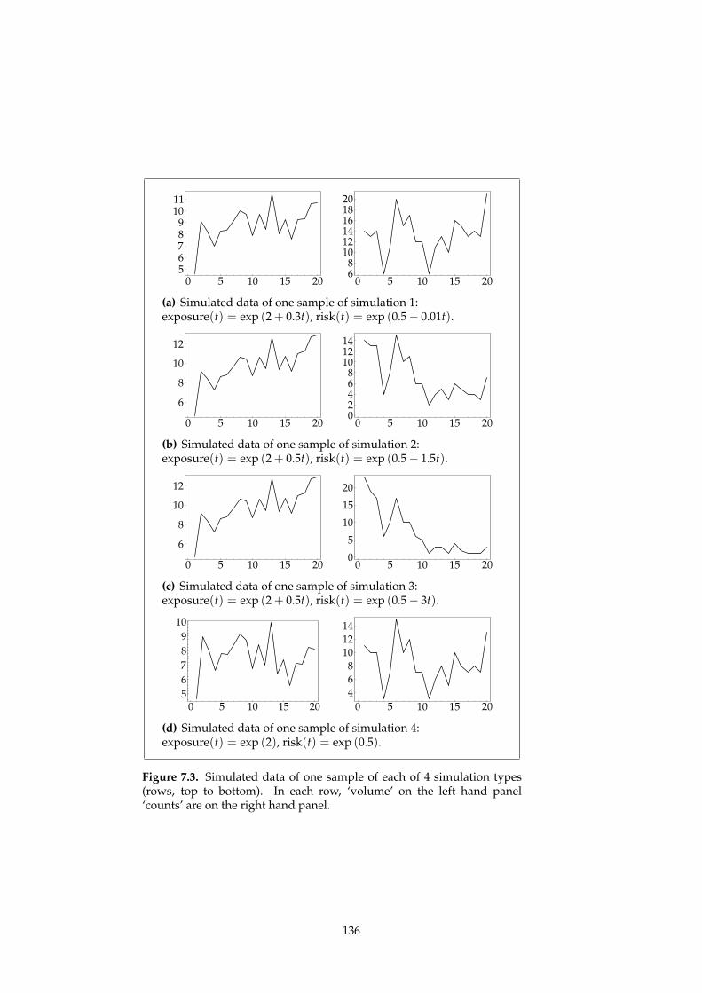
0 5 10 15 2056789
1011
0 5 10 15 2068
101214161820
(a) Simulated data of one sample of simulation 1:exposure(t) = exp (2 + 0.3t), risk(t) = exp (0.5 − 0.01t).
0 5 10 15 20
6
8
10
12
0 5 10 15 2002468
101214
(b) Simulated data of one sample of simulation 2:exposure(t) = exp (2 + 0.5t), risk(t) = exp (0.5 − 1.5t).
0 5 10 15 20
6
8
10
12
0 5 10 15 200
5
10
15
20
(c) Simulated data of one sample of simulation 3:exposure(t) = exp (2 + 0.5t), risk(t) = exp (0.5 − 3t).
0 5 10 15 205
6
7
8
9
10
0 5 10 15 20
4
68
101214
(d) Simulated data of one sample of simulation 4:exposure(t) = exp (2), risk(t) = exp (0.5).
Figure 7.3. Simulated data of one sample of each of 4 simulation types(rows, top to bottom). In each row, ‘volume’ on the left hand panel‘counts’ are on the right hand panel.
136

-2 -1 0 1 2 3
0.2
0.4
0.6
0.8
1
-2 -1 0 1 2 3
0.2
0.4
0.6
0.8
1
-2 -1 0 1 2 3
0.2
0.4
0.6
0.8
1
-2 -1 0 1 2 3
0.2
0.4
0.6
0.8
1
-2 -1 0 1 2 3
0.2
0.4
0.6
0.8
1
-2 -1 0 1 2 3
0.2
0.4
0.6
0.8
1
-2 -1 0 1 2 3
0.2
0.4
0.6
0.8
1
-2 -1 0 1 2 3
0.2
0.4
0.6
0.8
1
-2 -1 0 1 2 3
0.2
0.4
0.6
0.8
1
-2 -1 0 1 2 3
0.2
0.4
0.6
0.8
1
-2 -1 0 1 2 3
0.2
0.4
0.6
0.8
1
-2 -1 0 1 2 3
0.2
0.4
0.6
0.8
1
-2 -1 0 1 2 3
0.2
0.4
0.6
0.8
1
-2 -1 0 1 2 3
0.2
0.4
0.6
0.8
1
-2 -1 0 1 2 3
0.2
0.4
0.6
0.8
1
-2 -1 0 1 2 3
0.2
0.4
0.6
0.8
1
-2 -1 0 1 2 3
0.2
0.4
0.6
0.8
1
-2 -1 0 1 2 3
0.2
0.4
0.6
0.8
1
-2 -1 0 1 2 3
0.2
0.4
0.6
0.8
1
-2 -1 0 1 2 3
0.2
0.4
0.6
0.8
1
-2 -1 0 1 2 3
0.2
0.4
0.6
0.8
1
-2 -1 0 1 2 3
0.2
0.4
0.6
0.8
1
-2 -1 0 1 2 3
0.2
0.4
0.6
0.8
1
-2 -1 0 1 2 3
0.2
0.4
0.6
0.8
1
-2 -1 0 1 2 3
0.2
0.4
0.6
0.8
1
-2 -1 0 1 2 3
0.2
0.4
0.6
0.8
1
-2 -1 0 1 2 3
0.2
0.4
0.6
0.8
1
-2 -1 0 1 2 3
0.2
0.4
0.6
0.8
1
-2 -1 0 1 2 3
0.2
0.4
0.6
0.8
1
-2 -1 0 1 2 3
0.2
0.4
0.6
0.8
1
-2 -1 0 1 2 3
0.2
0.4
0.6
0.8
1
-2 -1 0 1 2 3
0.2
0.4
0.6
0.8
1
-2 -1 0 1 2 3
0.2
0.4
0.6
0.8
1
-2 -1 0 1 2 3
0.2
0.4
0.6
0.8
1
-2 -1 0 1 2 3
0.2
0.4
0.6
0.8
1
-2 -1 0 1 2 3
0.2
0.4
0.6
0.8
1
-2 -1 0 1 2 3
0.2
0.4
0.6
0.8
1
-2 -1 0 1 2 3
0.2
0.4
0.6
0.8
1
-2 -1 0 1 2 3
0.2
0.4
0.6
0.8
1
-2 -1 0 1 2 3
0.2
0.4
0.6
0.8
1
Figure 7.4. Cumulative plots of standardised errors over all samples of the last 10observations for simulation set 1. The dashed line denotes the cumulative function ofthe standard Gaussian distribution. The results for the ”level of log-exposure” (left),”slope of log-exposure”, ”level of log-risk” and ”slope of log-risk” (right) are arrangedhorizontally, while observation 11 through 20 are arranged downward.
137
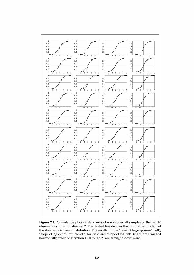
-2 -1 0 1 2 3
0.2
0.4
0.6
0.8
1
-2 -1 0 1 2 3
0.2
0.4
0.6
0.8
1
-2 -1 0 1 2 3
0.2
0.4
0.6
0.8
1
-2 -1 0 1 2 3
0.2
0.4
0.6
0.8
1
-2 -1 0 1 2 3
0.2
0.4
0.6
0.8
1
-2 -1 0 1 2 3
0.2
0.4
0.6
0.8
1
-2 -1 0 1 2 3
0.2
0.4
0.6
0.8
1
-2 -1 0 1 2 3
0.2
0.4
0.6
0.8
1
-2 -1 0 1 2 3
0.2
0.4
0.6
0.8
1
-2 -1 0 1 2 3
0.2
0.4
0.6
0.8
1
-2 -1 0 1 2 3
0.2
0.4
0.6
0.8
1
-2 -1 0 1 2 3
0.2
0.4
0.6
0.8
1
-2 -1 0 1 2 3
0.2
0.4
0.6
0.8
1
-2 -1 0 1 2 3
0.2
0.4
0.6
0.8
1
-2 -1 0 1 2 3
0.2
0.4
0.6
0.8
1
-2 -1 0 1 2 3
0.2
0.4
0.6
0.8
1
-2 -1 0 1 2 3
0.2
0.4
0.6
0.8
1
-2 -1 0 1 2 3
0.2
0.4
0.6
0.8
1
-2 -1 0 1 2 3
0.2
0.4
0.6
0.8
1
-2 -1 0 1 2 3
0.2
0.4
0.6
0.8
1
-2 -1 0 1 2 3
0.2
0.4
0.6
0.8
1
-2 -1 0 1 2 3
0.2
0.4
0.6
0.8
1
-2 -1 0 1 2 3
0.2
0.4
0.6
0.8
1
-2 -1 0 1 2 3
0.2
0.4
0.6
0.8
1
-2 -1 0 1 2 3
0.2
0.4
0.6
0.8
1
-2 -1 0 1 2 3
0.2
0.4
0.6
0.8
1
-2 -1 0 1 2 3
0.2
0.4
0.6
0.8
1
-2 -1 0 1 2 3
0.2
0.4
0.6
0.8
1
-2 -1 0 1 2 3
0.2
0.4
0.6
0.8
1
-2 -1 0 1 2 3
0.2
0.4
0.6
0.8
1
-2 -1 0 1 2 3
0.2
0.4
0.6
0.8
1
-2 -1 0 1 2 3
0.2
0.4
0.6
0.8
1
-2 -1 0 1 2 3
0.2
0.4
0.6
0.8
1
-2 -1 0 1 2 3
0.2
0.4
0.6
0.8
1
-2 -1 0 1 2 3
0.2
0.4
0.6
0.8
1
-2 -1 0 1 2 3
0.2
0.4
0.6
0.8
1
-2 -1 0 1 2 3
0.2
0.4
0.6
0.8
1
-2 -1 0 1 2 3
0.2
0.4
0.6
0.8
1
-2 -1 0 1 2 3
0.2
0.4
0.6
0.8
1
-2 -1 0 1 2 3
0.2
0.4
0.6
0.8
1
Figure 7.5. Cumulative plots of standardised errors over all samples of the last 10observations for simulation set 2. The dashed line denotes the cumulative function ofthe standard Gaussian distribution. The results for the ”level of log-exposure” (left),”slope of log-exposure”, ”level of log-risk” and ”slope of log-risk” (right) are arrangedhorizontally, while observation 11 through 20 are arranged downward.
138
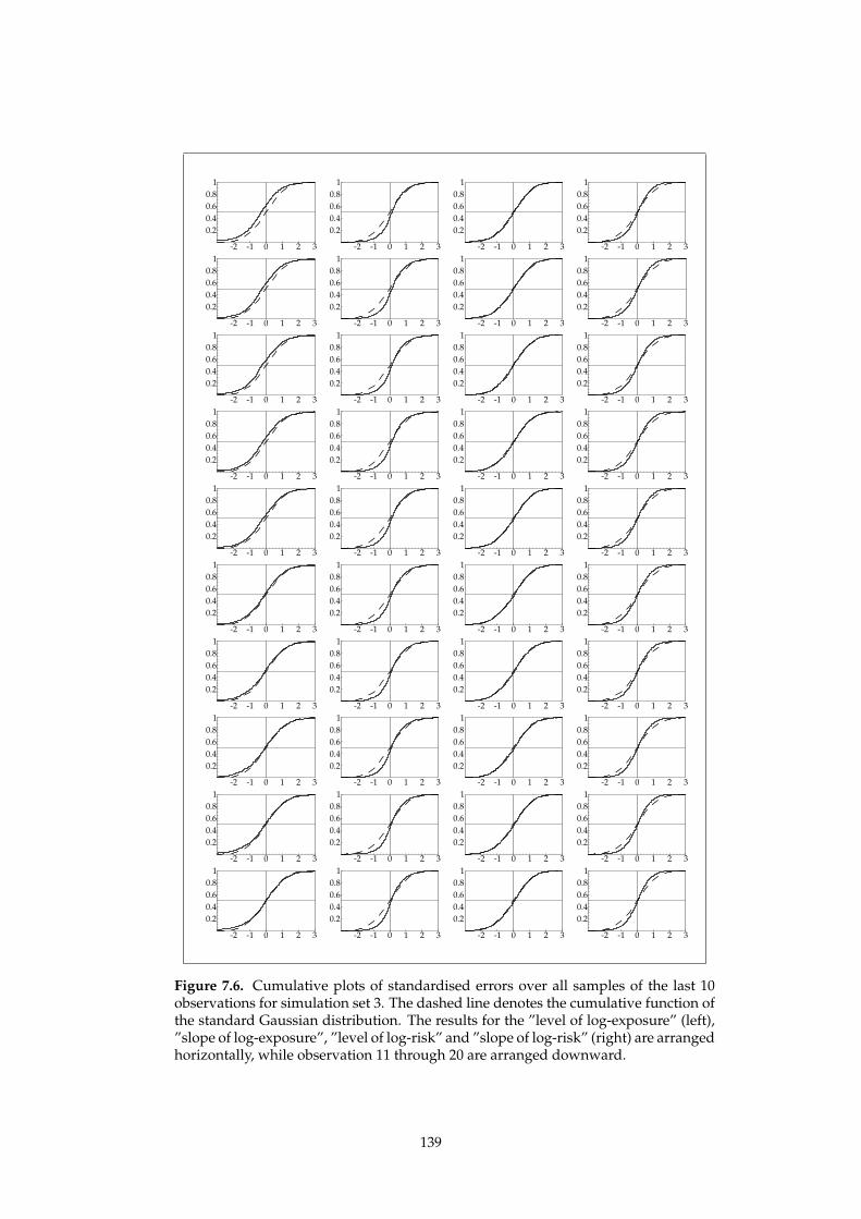
-2 -1 0 1 2 3
0.2
0.4
0.6
0.8
1
-2 -1 0 1 2 3
0.2
0.4
0.6
0.8
1
-2 -1 0 1 2 3
0.2
0.4
0.6
0.8
1
-2 -1 0 1 2 3
0.2
0.4
0.6
0.8
1
-2 -1 0 1 2 3
0.2
0.4
0.6
0.8
1
-2 -1 0 1 2 3
0.2
0.4
0.6
0.8
1
-2 -1 0 1 2 3
0.2
0.4
0.6
0.8
1
-2 -1 0 1 2 3
0.2
0.4
0.6
0.8
1
-2 -1 0 1 2 3
0.2
0.4
0.6
0.8
1
-2 -1 0 1 2 3
0.2
0.4
0.6
0.8
1
-2 -1 0 1 2 3
0.2
0.4
0.6
0.8
1
-2 -1 0 1 2 3
0.2
0.4
0.6
0.8
1
-2 -1 0 1 2 3
0.2
0.4
0.6
0.8
1
-2 -1 0 1 2 3
0.2
0.4
0.6
0.8
1
-2 -1 0 1 2 3
0.2
0.4
0.6
0.8
1
-2 -1 0 1 2 3
0.2
0.4
0.6
0.8
1
-2 -1 0 1 2 3
0.2
0.4
0.6
0.8
1
-2 -1 0 1 2 3
0.2
0.4
0.6
0.8
1
-2 -1 0 1 2 3
0.2
0.4
0.6
0.8
1
-2 -1 0 1 2 3
0.2
0.4
0.6
0.8
1
-2 -1 0 1 2 3
0.2
0.4
0.6
0.8
1
-2 -1 0 1 2 3
0.2
0.4
0.6
0.8
1
-2 -1 0 1 2 3
0.2
0.4
0.6
0.8
1
-2 -1 0 1 2 3
0.2
0.4
0.6
0.8
1
-2 -1 0 1 2 3
0.2
0.4
0.6
0.8
1
-2 -1 0 1 2 3
0.2
0.4
0.6
0.8
1
-2 -1 0 1 2 3
0.2
0.4
0.6
0.8
1
-2 -1 0 1 2 3
0.2
0.4
0.6
0.8
1
-2 -1 0 1 2 3
0.2
0.4
0.6
0.8
1
-2 -1 0 1 2 3
0.2
0.4
0.6
0.8
1
-2 -1 0 1 2 3
0.2
0.4
0.6
0.8
1
-2 -1 0 1 2 3
0.2
0.4
0.6
0.8
1
-2 -1 0 1 2 3
0.2
0.4
0.6
0.8
1
-2 -1 0 1 2 3
0.2
0.4
0.6
0.8
1
-2 -1 0 1 2 3
0.2
0.4
0.6
0.8
1
-2 -1 0 1 2 3
0.2
0.4
0.6
0.8
1
-2 -1 0 1 2 3
0.2
0.4
0.6
0.8
1
-2 -1 0 1 2 3
0.2
0.4
0.6
0.8
1
-2 -1 0 1 2 3
0.2
0.4
0.6
0.8
1
-2 -1 0 1 2 3
0.2
0.4
0.6
0.8
1
Figure 7.6. Cumulative plots of standardised errors over all samples of the last 10observations for simulation set 3. The dashed line denotes the cumulative function ofthe standard Gaussian distribution. The results for the ”level of log-exposure” (left),”slope of log-exposure”, ”level of log-risk” and ”slope of log-risk” (right) are arrangedhorizontally, while observation 11 through 20 are arranged downward.
139

-2 -1 0 1 2 3
0.2
0.4
0.6
0.8
1
-2 -1 0 1 2 3
0.2
0.4
0.6
0.8
1
-2 -1 0 1 2 3
0.2
0.4
0.6
0.8
1
-2 -1 0 1 2 3
0.2
0.4
0.6
0.8
1
-2 -1 0 1 2 3
0.2
0.4
0.6
0.8
1
-2 -1 0 1 2 3
0.2
0.4
0.6
0.8
1
-2 -1 0 1 2 3
0.2
0.4
0.6
0.8
1
-2 -1 0 1 2 3
0.2
0.4
0.6
0.8
1
-2 -1 0 1 2 3
0.2
0.4
0.6
0.8
1
-2 -1 0 1 2 3
0.2
0.4
0.6
0.8
1
-2 -1 0 1 2 3
0.2
0.4
0.6
0.8
1
-2 -1 0 1 2 3
0.2
0.4
0.6
0.8
1
-2 -1 0 1 2 3
0.2
0.4
0.6
0.8
1
-2 -1 0 1 2 3
0.2
0.4
0.6
0.8
1
-2 -1 0 1 2 3
0.2
0.4
0.6
0.8
1
-2 -1 0 1 2 3
0.2
0.4
0.6
0.8
1
-2 -1 0 1 2 3
0.2
0.4
0.6
0.8
1
-2 -1 0 1 2 3
0.2
0.4
0.6
0.8
1
-2 -1 0 1 2 3
0.2
0.4
0.6
0.8
1
-2 -1 0 1 2 3
0.2
0.4
0.6
0.8
1
-2 -1 0 1 2 3
0.2
0.4
0.6
0.8
1
-2 -1 0 1 2 3
0.2
0.4
0.6
0.8
1
-2 -1 0 1 2 3
0.2
0.4
0.6
0.8
1
-2 -1 0 1 2 3
0.2
0.4
0.6
0.8
1
-2 -1 0 1 2 3
0.2
0.4
0.6
0.8
1
-2 -1 0 1 2 3
0.2
0.4
0.6
0.8
1
-2 -1 0 1 2 3
0.2
0.4
0.6
0.8
1
-2 -1 0 1 2 3
0.2
0.4
0.6
0.8
1
-2 -1 0 1 2 3
0.2
0.4
0.6
0.8
1
-2 -1 0 1 2 3
0.2
0.4
0.6
0.8
1
-2 -1 0 1 2 3
0.2
0.4
0.6
0.8
1
-2 -1 0 1 2 3
0.2
0.4
0.6
0.8
1
-2 -1 0 1 2 3
0.2
0.4
0.6
0.8
1
-2 -1 0 1 2 3
0.2
0.4
0.6
0.8
1
-2 -1 0 1 2 3
0.2
0.4
0.6
0.8
1
-2 -1 0 1 2 3
0.2
0.4
0.6
0.8
1
-2 -1 0 1 2 3
0.2
0.4
0.6
0.8
1
-2 -1 0 1 2 3
0.2
0.4
0.6
0.8
1
-2 -1 0 1 2 3
0.2
0.4
0.6
0.8
1
-2 -1 0 1 2 3
0.2
0.4
0.6
0.8
1
Figure 7.7. Cumulative plots of standardised errors over all samples for of the last10 observations simulation set 4. The dashed line denotes the cumulative function ofthe standard Gaussian distribution. The results for the ”level of log-exposure” (left),”slope of log-exposure”, ”level of log-risk” and ”slope of log-risk” (right) are arrangedhorizontally, while observation 11 through 20 are arranged downward.
140

variance appears to be sufficiently correct. The slopes did not fare so well. In
particular in the second column, which represents the distribution of the slope
of the log-exposure component, the distributions appear skewed (dashed line
over the empirical cumulative distribution in the negative horizontal range,
while less difference is visible in the positive range), and it appears that the
distributions for the slope of the log-risk component (fourth column) have less
variance than is expected. This could be the result of the estimate of the var-
iance of the component being generally too large. In road safety analysis in-
ference has most often to be drawn from log-exposure and log-risk estimate
(the third and first column). Based on this particular simulation experiment
the performance of the likelihoodfilter approach in reconstructing the risk and
exposure processes in a typical road safety application appears to be accept-
able.
7.5. Applications
7.5.1. Volatility: pound/dollar daily exchange rates
This application re-estimates a zero-mean stochastic volatility model as de-
scribed in Durbin and Koopman (2001), see also Harvey, Ruiz, and Shephard
(1994). Following Durbin and Koopman (2001), denoting the daily exchange
rate by xt, the observations considered are given by yt = △ log(xt), for t =
1, . . . , n. The following model is considered (t = 1, . . . , n, 0 < φ < 1):
yt =σ exp
(
1
2θt
)
ut, ut ∼ N(0, 1),
θt+1 =φθt + ηt, ηt ∼ N(0, σ2η).
(7.22)
In order to allow for unconstrained optimisation techniques, the parameters
σ, ση and φ are internally represented as σ = exp(ψ1), ση = exp(ψ2), and
ψ = exp(ψ3)/(1 + exp(ψ3)). The method used by Durbin and Koopman
(2001) resulted in the estimates given on the left hand side of Table 7.8. The
likelihoodfilter results are given on the right hand side. Given the fact that the
results reported by Lee and Nelder (2006) are quite similar to the results re-
ported by Durbin and Koopman (2001), and that the results derived from the
likelihoodfilter differ from these (although not significantly), we conclude that
the performance of the likelihoodfilter is acceptable, although a more detailed
study is needed to assess the method.
141

Durbin and Koopman (2001) Likelihoodfilterinternal internal internal
estimate representation estimate estimate estimate
σ = 0.6338 σ = exp(ψ1) ψ1=-0.4561 σ = 0.7053 ψ1=-0.3491(0.1033) (0.1203)
ση = 0.1726 ση = exp(ψ2) ψ2=-1.7569 ση = 0.1902 ψ2=-1.65991(0.2170) (0.2253)
φ = 0.9731 φ =exp(ψ3)
1+exp(ψ3)ψ3= 3.5876 φ = 0.9691 ψ3=3.44713
(0.5007) (0.4815)
Figure 7.8. Parameter estimates and standard deviations for the stochastic volatilitymodel compared. Both real-world and internal representation of the parameter esti-mates due to Durbin and Koopman (2001) on the left hand and the likelihood filteron the right hand are given. The internal representations are used to constrain σ, ση
and φ to: σ > 0, ση > 0 and 0 < φ < 1.
7.5.2. The effects of precipitation on road safety
Introduction
It is commonly assumed that weather conditions influence the occurrence of
accidents in road traffic. The nature of the established and suspected influences
is diverse, including direct effects like poor visibility and deteriorated road
surface conditions impairing the capabilities of road users to avoid accidents,
and indirect effects like the decision to travel, choice of travel time and means
of transport influencing the number of road users at risk.
A common approach taken in road safety analysis is to compare the number of
accidents corrected for the amount of traffic – often called risk – under the dif-
ferent weather conditions. This approach however is not as straightforward to
implement as it may seem to be. First of all, data availability may induce lim-
itations, and often it will be difficult to determine the amount of traffic under
the different weather conditions. In previous studies, several approaches are
taken to obtain comparable accident counts, recognising differences in traffic
volume. Often days (or parts as in Andrey and Yagar (1993)) with precipitation
are matched with otherwise comparable days without precipitation, separated
by a short period of time, usually a week. This approach is more likely to se-
lect observations in periods with volatile weather conditions than from stable,
summer weather periods. This may cause bias issues. For an extensive discus-
sion of the influence of precipitation on road safety refer to for instance Brod-
sky and Hakkert (1988); Eisenberg (2004); Keay and Simmonds (2005, 2006)
and the references therein.
142
The following application describes a model currently under development de-
signed to identify an (potentially) increased ratio of the number of accidents
per traffic kilometre (risk) under wet weather conditions compared to dry
weather conditions in the Netherlands. For reasons beyond the scope of an
example in this article, the accident type is restricted to single fatal car acci-
dents. This type of accident is relatively well registered, and travel volume of
cars appears mildly influenced by immediate weather conditions, compared
to for instance bicyclists who may take shelter from a rain storm. This latter
aspect is important as we want to aggregate observations to the daily level
and compare the number of accidents with and without precipitation to an es-
timate of travel with and without precipitation, similar to the corrected ‘wet
pavement index’ as described by Brodsky and Hakkert (1988).
The following data is available:
• weather data provided by the Royal Netherlands Meteorological Institute
(KNMI, 2006) for a number of weather stations distributed over the Neth-
erlands. On the KNMI (2006) website, highly detailed data is available for
10 weather stations spanning a sufficiently long time. The observations
are on a daily (in universal time) basis (daily sums, averages, maxima
and minima) on a number of indicators. To start building a model in this
study, the duration of precipitation is used, as measured in the number
of units of one tenth of an hour, see Figure 7.9.
• detailed traffic volume data for most modes of transport (including cars)
is provided in a consistent manner since 1985 from the Dutch national
travel survey (CBS, 2003; AVV, 2005). Although starting and ending lo-
cation and time of trips as reported by interviewed Dutch inhabitants
are often known, it appears impossible to determine the parts of the trip
undertaken under the respective weather conditions. Data on travel kilo-
metres by car drivers is used, see Figure 7.9.
• detailed accident data is provided in a consistent dataset as of 1987 (older
data is available) (AVV, 2006) from which the weather conditions of the
accidents are determined through the police records rather than accident
location and time. Weather conditions in the accident record are un-
known for about 3% of the fatal accidents, which are further discarded
from this analysis. Counts of fatal single car accidents are used, see Fig-
ure 7.9.
143

1987/1/1 1993/5/2 1999/9/1 2005/12/30
5101520
1987/1/1 1993/5/2 1999/9/1 2005/12/30
5101520
1987/1/1 1993/5/2 1999/9/1 2005/12/30
0.20.40.60.81.0
1987/1/1 1993/5/2 1999/9/1 2005/12/30
50100150200
Figure 7.9. Available data: Top left: number of dry weather accidents; top right:number of wet weather accidents (both fatal single car accidents); bottom left:traffic volume (car driver kilometres). The survey was substantially extended in1994, but later somewhat reduced; bottom right: precipitation duration in ‘DeKooy’ 6-minute units.
Although more detailed data are available, it is decided to restrict the analysis
to the daily level at this point of model development, both to limit the size of
the model and to avoid data compatibility issues: accident times as recorded
by the police tend to be rounded to the (probably) nearest full hour, half hour,
quarter of an hour, ten and five minute points. The extent of this issue is under
investigation in a separate study matching accident data to ambulance data
that do not observe this phenomenon. Published weather data however is ag-
gregated over minutes 0 − 59. The travel survey data observe this time round-
ing phenomenon even in a stronger manner. Therefore, acknowledging the
locality in space and time of for instance rainfall (Brodsky and Hakkert, 1988),
we feel the advantages of using hourly instead of daily data may be limited,
and start development using daily data.
In this study, an approach to estimating the traffic volume – and subsequently
risk – under ‘dry’ and ‘wet’ weather conditions similar to Bijleveld et al. (2008)
is developed. To that end, a latent component for general risk as well as a latent
component for the relative risk under wet weather conditions is defined. In
addition, a latent component for the total travel volume is defined. This total
travel volume is distributed over ‘dry’ and ‘wet’ weather conditions by means
of an estimate of the fraction of travel with precipitation. In order for this
assumption to be reasonable, it is necessary to be allowed to assume that travel
is not influenced too much by precipitation. This appears to be the case with
travel by cars. The topic of the impact of weather conditions on travel habits
in general (for other means of transport) is the subject of further research. This
is one of the reasons to restrict the analysis to the safety of cars.
144

The fraction of travel with precipitation is derived as follows. First it is as-
sumed that for a small country like the Netherlands the daily fraction of travel
with precipitation represents the average fraction of time with precipitation
well. It is assumed that no considerable structural differences in the weather
pattern exist,29 although regional variation may apply. The daily fraction of
travel with precipitation is not directly observed and is therefore further con-
sidered a latent factor. The precipitation duration for the 10 weather stations
however is measured and used in this analysis. The mechanism by which the
data is collected is quite accurate, but the data is rounded. Each of these obser-
vations is considered a random draw from a Gaussian distribution with mean
equal to a given fraction of travel with precipitation, and a variance considering
the direct measurement error, the fact that universal time days are used while
other data is in middle European time (a one or two hour lag, depending on
winter or summer time) which introduces another error, and the error due to
regional differences in weather conditions. The magnitude of the combined
variance is assumed the same for the whole period. We will consider the dy-
namic aspects of this latent factor as common sense suggests that the weather
today has some predictive value for the weather tomorrow. An optimal pre-
diction is likely to depend on conditions like air-pressure, direction of wind
(wind from sea or not) and (average) temperature. Variables measuring such
influences are not included in the model. In our initial development efforts,
without such explanatory variables, a local level model is considered for an
inverse logistic transformed version of this series.
Similar to Bijleveld et al. (2008), it is not assumed that the volume of the traffic
itself is what is causing accidents, rather we assume that a latent, unobserv-
able traffic process exists, on average proportional to the exposure to accidents
and on average proportional to – but not identical to – the traffic volume. We
further assume the measurement of the daily traffic volume to be subject to
(substantial survey) error (Slootbeek, 1993). Using an exponential transform
to maintain positiveness, we have:
Total traffic volume = exp(exposure) + error (7.23)
The following general accident model for dry and wet weather conditions is
under consideration, where f is the fraction of travel under ‘wet’ weather con-
29We can however not be certain about this. Small, at first sight unimportant differencesmay turn out to be relevant to road safety, but at this point we do not know.
145
ditions (suppressing the time index for clarity):
Number of accidentsdry = exp(exposure) × (1 − f ) × Riskgeneral (7.24)
Number of accidentswet = exp(exposure) × f × Riskgeneral × Riskwet,
(7.25)
where ultimately Riskwet is of most interest.
Details: observation model
In more detail, the following observation model will now be considered. We
first define – using Latin capitals for observed values – the number of dry
weather accidents at day t by Dt, the number of wet weather accidents at day
t by Wt, the total traffic volume (car driver kilometres) as Vt (error variance
estimate σ2(Vt)) and the number of tenth-hours of the day with precipitation
for each weather station i, recoded into the fraction of time with precipitation
F(i)t , where 0 ≤ F
(i)t < 1 (it never rains all day) and i = 1, . . . , 10. We assume
– using lower case Latin symbols for latent factors – a latent log-general risk
factor (r(g)t ) and log-relative risk wet weather conditions factor (r
(w)t ) as well
as a latent factor (vt) for log-exposure. Finally we have an unobserved com-
ponent ft, the logistic transformation of which determines the fraction of the
traffic with precipitation that day. Given ft (which is stochastic), the fraction of
time with precipitation for each weather station is assumed to follow an inde-
pendent Gaussian distribution with mean 1/(1 + exp(− ft)) and variance equal
to a constant σ2(Ft) plus an estimated parameter σ2F. Technically, the indepen-
dence assumption is not likely to truly hold, as spacial relations should be
considered. However, this effect is ignored at this point, but when knowledge
about its structure is available, it could be incorporated in the model without
too much effort.
Further we assume the accident counts to be independently Poisson distributed
given the latent factors while, given the latent factors, the traffic volume is inde-
pendently Gaussian distributed with variance determined by the travel survey
plus potential extra variance.
146

The log-likelihood of an observation Yt = {Dt, Wt, Vt, F(1)t , . . . , F
(10)t }, given the
latent factors at = {vt, ft, r(g)t , r
(w)t }, is now:
l(Yt|at) = logPoisson(
Dt, λ := 1/(1 + exp( ft)) exp (vt + r(g)t )
)
+
(7.26)
logPoisson(
Wt, λ := 1/(1 + exp(− ft)) exp(
vt + r(g) + r(w)t
))
+
(7.27)
LogGaussian(
Vt, µ := exp (vt), σ2 := σ2(Vt) + σ2V
)
+ (7.28)
10
∑i=1
LogGaussian(F(i)t , µ := 1/(1 + exp(− ft)), σ2 := σ2(Ft) + σ2
F).
(7.29)
This approach, where latent variables and both continuous and discrete de-
pendent variables are modelled can also be found in Sammel, Ryan, and Legler
(1997).
Details: dynamics model
At this stage of model development, the latent factors {vt, ft, r(g)t , r
(w)t } are as-
sumed to be related over time, acknowledging that in the future, at least in
theory, this time variation may be (in part) explained by yet unidentified ex-
planatory variables. For now, all latent factors except the fraction of time with
precipitation ft are modelled using a basic structural model with ‘seasonal’
component Harvey (1989, Chapter 6–7). The ‘seasonal’ component however is
used to model the weekly patterns in traffic volume, as well as the apparent
weekly pattern in the risk components. The fraction of traffic with precipi-
tation related component ft is for now modelled using a local level model.
Obviously, explanatory variables like average air pressure, humidity and tem-
perature as well as travel variables are likely to improve the explanation of the
development of the fraction of travel with precipitation component ft. How-
ever, such improvements are not likely to change the general model structure,
which is studied here.
The dynamical specification of a basic structural model with a ‘seasonal’ of
length seven (for a week) is in general defined as follows (Harvey, 1989, Chap-
147
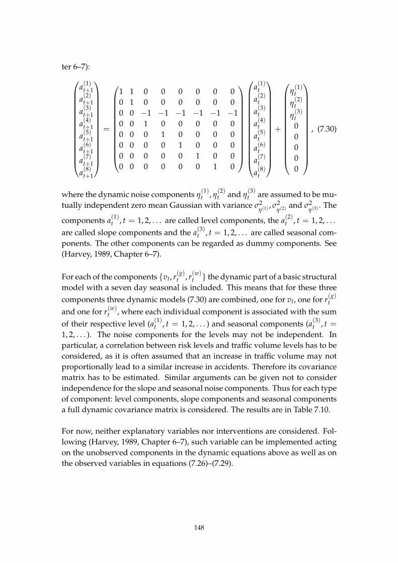
ter 6–7):
a(1)t+1
a(2)t+1
a(3)t+1
a(4)t+1
a(5)t+1
a(6)t+1
a(7)t+1
a(8)t+1
=
1 1 0 0 0 0 0 0
0 1 0 0 0 0 0 0
0 0 −1 −1 −1 −1 −1 −1
0 0 1 0 0 0 0 0
0 0 0 1 0 0 0 0
0 0 0 0 1 0 0 0
0 0 0 0 0 1 0 0
0 0 0 0 0 0 1 0
a(1)t
a(2)t
a(3)t
a(4)t
a(5)t
a(6)t
a(7)t
a(8)t
+
η(1)t
η(2)t
η(3)t
0
0
0
0
0
, (7.30)
where the dynamic noise components η(1)t , η
(2)t and η
(3)t are assumed to be mu-
tually independent zero mean Gaussian with variance σ2η(1) , σ2
η(2) and σ2η(3) . The
components a(1)t , t = 1, 2, . . . are called level components, the a
(2)t , t = 1, 2, . . .
are called slope components and the a(3)t , t = 1, 2, . . . are called seasonal com-
ponents. The other components can be regarded as dummy components. See
(Harvey, 1989, Chapter 6–7).
For each of the components {vt, r(g)t , r
(w)t } the dynamic part of a basic structural
model with a seven day seasonal is included. This means that for these three
components three dynamic models (7.30) are combined, one for vt, one for r(g)t
and one for r(w)t , where each individual component is associated with the sum
of their respective level (a(1)t , t = 1, 2, . . . ) and seasonal components (a
(3)t , t =
1, 2, . . . ). The noise components for the levels may not be independent. In
particular, a correlation between risk levels and traffic volume levels has to be
considered, as it is often assumed that an increase in traffic volume may not
proportionally lead to a similar increase in accidents. Therefore its covariance
matrix has to be estimated. Similar arguments can be given not to consider
independence for the slope and seasonal noise components. Thus for each type
of component: level components, slope components and seasonal components
a full dynamic covariance matrix is considered. The results are in Table 7.10.
For now, neither explanatory variables nor interventions are considered. Fol-
lowing (Harvey, 1989, Chapter 6–7), such variable can be implemented acting
on the unobserved components in the dynamic equations above as well as on
the observed variables in equations (7.26)–(7.29).
148
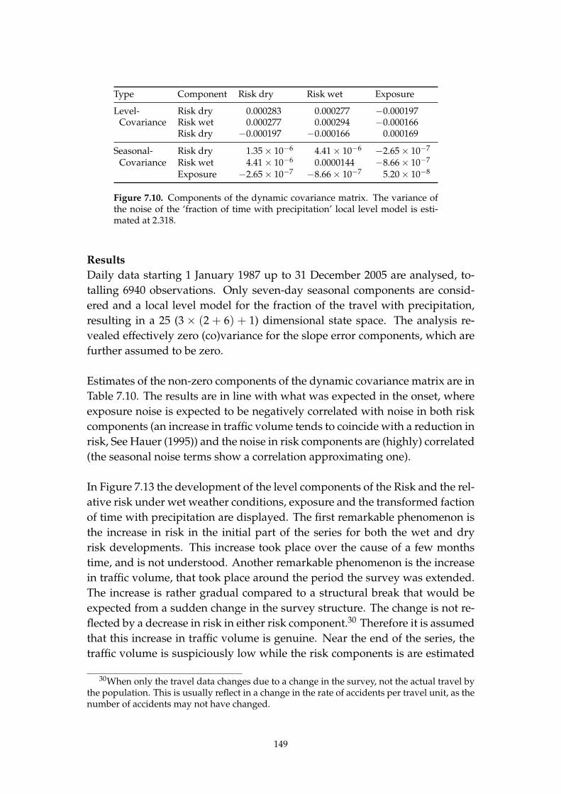
Type Component Risk dry Risk wet Exposure
Level- Risk dry 0.000283 0.000277 −0.000197Covariance Risk wet 0.000277 0.000294 −0.000166
Risk dry −0.000197 −0.000166 0.000169
Seasonal- Risk dry 1.35 × 10⁻⁶ 4.41 × 10⁻⁶ −2.65 × 10⁻⁷
Covariance Risk wet 4.41 × 10⁻⁶ 0.0000144 −8.66 × 10⁻⁷
Exposure −2.65 × 10⁻⁷ −8.66 × 10⁻⁷ 5.20 × 10⁻⁸
Figure 7.10. Components of the dynamic covariance matrix. The variance ofthe noise of the ‘fraction of time with precipitation’ local level model is esti-mated at 2.318.
Results
Daily data starting 1 January 1987 up to 31 December 2005 are analysed, to-
talling 6940 observations. Only seven-day seasonal components are consid-
ered and a local level model for the fraction of the travel with precipitation,
resulting in a 25 (3 × (2 + 6) + 1) dimensional state space. The analysis re-
vealed effectively zero (co)variance for the slope error components, which are
further assumed to be zero.
Estimates of the non-zero components of the dynamic covariance matrix are in
Table 7.10. The results are in line with what was expected in the onset, where
exposure noise is expected to be negatively correlated with noise in both risk
components (an increase in traffic volume tends to coincide with a reduction in
risk, See Hauer (1995)) and the noise in risk components are (highly) correlated
(the seasonal noise terms show a correlation approximating one).
In Figure 7.13 the development of the level components of the Risk and the rel-
ative risk under wet weather conditions, exposure and the transformed faction
of time with precipitation are displayed. The first remarkable phenomenon is
the increase in risk in the initial part of the series for both the wet and dry
risk developments. This increase took place over the cause of a few months
time, and is not understood. Another remarkable phenomenon is the increase
in traffic volume, that took place around the period the survey was extended.
The increase is rather gradual compared to a structural break that would be
expected from a sudden change in the survey structure. The change is not re-
flected by a decrease in risk in either risk component.30 Therefore it is assumed
that this increase in traffic volume is genuine. Near the end of the series, the
traffic volume is suspiciously low while the risk components is are estimated
30When only the travel data changes due to a change in the survey, not the actual travel bythe population. This is usually reflect in a change in the rate of accidents per travel unit, as thenumber of accidents may not have changed.
149
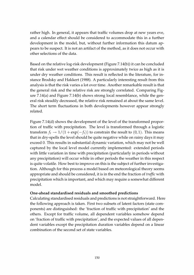
rather high. In general, it appears that traffic volumes drop at new years eve,
and a calendar effect should be considered to accommodate this in a further
development in the model, but, without further information this datum ap-
pears to be suspect. It is not an artifact of the method, as it does not occur with
other selections of the data.
Based on the relative log-risk development (Figure 7.14(b)) it can be concluded
that risk under wet weather conditions is approximately twice as high as it is
under dry weather conditions. This result is reflected in the literature, for in-
stance Brodsky and Hakkert (1988). A particularly interesting result from this
analysis is that the risk varies a lot over time. Another remarkable result is that
the general risk and the relative risk are strongly correlated. Comparing Fig-
ure 7.14(a) and Figure 7.14(b) shows strong local resemblance, while the gen-
eral risk steadily decreased, the relative risk remained at about the same level.
The short term fluctuations in both developments however appear strongly
related.
Figure 7.14(d) shows the development of the level of the transformed propor-
tion of traffic with precipitation. The level is transformed through a logistic
transform ft → 1/(1 + exp(− ft)) to constrain the result to (0, 1). This means
that in dry-spells the level should be quite negative while on rainy days it may
exceed 0. This results in substantial dynamic variation, which may not be well
captured by the local level model currently implemented: extended periods
with little variation in time with precipitation (particularly in periods without
any precipitation) will occur while in other periods the weather in this respect
is quite volatile. How best to improve on this is the subject of further investiga-
tion. Although for this process a model based on meteorological theory seems
appropriate and should be considered, it is in the end the fraction of traffic with
precipitation which is important, and which may require a somewhat different
model.
One-ahead standardised residuals and smoothed predictions
Calculating standardised residuals and predictions is not straightforward. Here
the following approach is taken. First two subsets of latent factors (state com-
ponents) are distinguished: the ‘fraction of traffic with precipitation’ and the
others. Except for traffic volume, all dependent variables somehow depend
on ‘fraction of traffic with precipitation’, and the expected values of all depen-
dent variables except the precipitation duration variables depend on a linear
combination of the second set of state variables.
150

1987/1/1 1993/5/2 1999/9/1 2005/12/302.4
2.6
2.8
3.0
3.2
3.4
3.6
(a) Level log Risk
1987/1/1 1993/5/2 1999/9/1 2005/12/30
0.4
0.6
0.8
1.0
1.2
(b) Level log Relative Risk Wet
1987/1/1 1993/5/2 1999/9/1 2005/12/30
-2.0-1.9-1.8-1.7-1.6-1.5-1.4-1.3
(c) Level log Exposure
1987/1/1 1993/5/2 1999/9/1 2005/12/30-12-10 -8 -6 -4 -2 0 2
(d) Inverse logistic ‘fraction wet’
Figure 7.13. Development of selected latent factors, including pointwise 95%margins.
151
For instance, the expected number of wet weather accidents is by (7.27)
1/(1 + exp(− ft)) exp(
vt + r(g)t + r
(w)t
)
which can be further simplified into
1/(1 + exp(−x)) exp (y) (7.31)
where (x, y) is assumed bi-variate Gaussian, its expected value and covariance
determined from the one-ahead predicted state or smoothed state depending
on purpose. The predictions are determined by evaluating the expected value
of (7.31) under bi-variate Gaussian law. The variance is calculated by adding
the prediction to the variance of (7.31). Smoothed predictions and one-ahead
predictions of traffic volume data and precipitation duration data are deter-
mined in a similar, less complicated manner.
The residuals (omitted for the ten weather stations), depicted in Figure 7.16 do
not appear to be Gaussian. The turning points test is non-significant for the
dry weather accidents and almost significant for the traffic volume. The test
is significant for the wet weather accidents. These residuals also show a sig-
nificant negative first-order autocorrelation. This result appears to be in line
with findings of Eisenberg (2004), where 1 cm of precipitation if found to be
associated with a decrease of 3.06% the next day, while 1 cm of rain is associ-
ated with an increase of 1.83% of accidents on the same day. So the fact that
it rained the previous day reduces the number of accidents today. However,
these results are for the total number of fatal accidents (irrespective of weather
conditions) and exposure is based on the annual motor vehicle kilometres.
Relative risk
Probably the most interesting results can be obtained studying the smoothed
log risk developments in Figure 7.14(a) (general risk) and 7.14(b) (Relative risk
weather under precipitation). Their joint development could be studied in or-
der to identify general influences on road safety, however, focus is directed at
precipitation effects. One obvious choice is then to calculate the relative risk
under wet conditions. In Figure 7.20 the relative risk (the exponential trans-
form of the relative log-risk under wet weather conditions) and its margins is
given.
It is clear from Figure 7.20, that the risk in traffic increases by a factor of two
when precipitation is present. However, given that, it is also clear that substan-
tial differences exist. In Figure 7.20, fluctuations in the level of the relative risk
are smoothed, but it is obvious that the level is sometimes lower and some-
152

1987/1/1 1993/5/2 1999/9/1 2005/12/30
-2
-1
0
1
2
3
4
(a) Residuals fatal dry weather single car accidents
1987/1/1 1993/5/2 1999/9/1 2005/12/30
-0.6
-0.4
-0.2
0.0
0.2
0.4
(b) Residuals fatal wet weather single car accidents
1987/1/1 1993/5/2 1999/9/1 2005/12/30
-4
-2
0
2
(c) Residuals car traffic volume
Figure 7.16. One ahead standardised residuals.
153
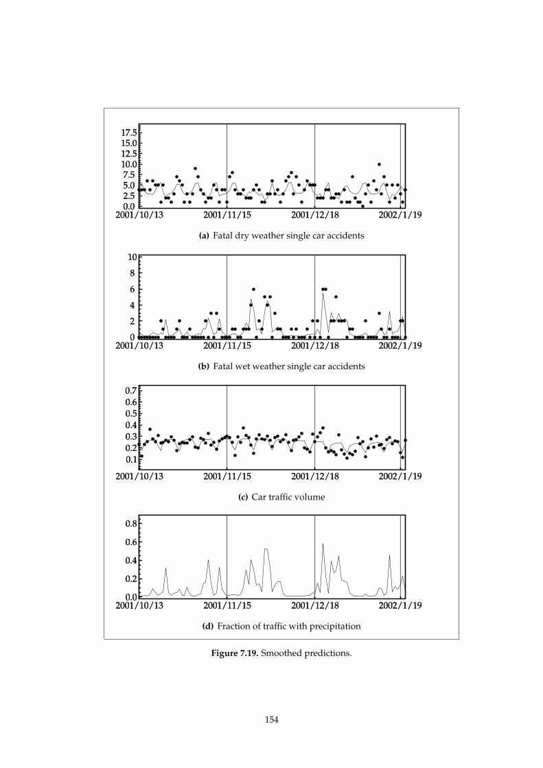
2001/10/13 2001/11/15 2001/12/18 2002/1/19 0.0 2.5 5.0 7.5
10.012.515.017.5
2001/10/13 2001/11/15 2001/12/18 2002/1/19 0.0 2.5 5.0 7.5
10.012.515.017.5
(a) Fatal dry weather single car accidents
2001/10/13 2001/11/15 2001/12/18 2002/1/19 0
2
4
6
8
10
2001/10/13 2001/11/15 2001/12/18 2002/1/19 0
2
4
6
8
10
(b) Fatal wet weather single car accidents
2001/10/13 2001/11/15 2001/12/18 2002/1/19
0.10.20.30.40.50.60.7
2001/10/13 2001/11/15 2001/12/18 2002/1/19
0.10.20.30.40.50.60.7
(c) Car traffic volume
2001/10/13 2001/11/15 2001/12/18 2002/1/190.0
0.2
0.4
0.6
0.8
2001/10/13 2001/11/15 2001/12/18 2002/1/190.0
0.2
0.4
0.6
0.8
(d) Fraction of traffic with precipitation
Figure 7.19. Smoothed predictions.
154

1987/1/1 1993/5/2 1999/9/1 2005/12/30
1.5
2.0
2.5
3.0
Figure 7.20. Smoothed log relative risk wet weather conditions versus dryweather conditions.
times higher than average. A next step in model development should be to
relate these variations to external influences, like precipitation intensity, tem-
perature, but also non-meteorological factors. A similar effort should be taken
with respect to the joint risk development, as well as the traffic volume distri-
bution.
7.5.3. Conclusions
Based on the relative risk development it can be concluded that risk under wet
weather conditions is approximately twice as high as it is under dry weather
conditions. This result is reflected in the literature. A particularly interesting
result from this analysis is that the risk varies a lot over time. Another remark-
able result is that the general risk and the relative risk are strongly correlated.
Comparing Figure 7.14(a) and Figure 7.14(b) show strong local resemblance,
while the general risk steadily decreased, the relative risk basically remained
at the same level. That aside, the short term fluctuations in both developments
appear strongly related. If the results are correct, this suggests that one pro-
cess may govern both variations, although the relative risk appears to be more
sensitive to this process.
7.6. Discussion and conclusions
An approach to filtering and likelihood estimation for state space models where
the dependent variables can have a non-Gaussian distribution is considered.
The state space however is still assumed to be rule by Gaussian disturbances.
The approach considered can be regarded as generalisation of the iterated ex-
tended Kalman filter, therefore it shares its properties. It appears to function
well in the Gaussian-Poisson combination described in the simulation stud-
ies in Section 7.4, but did not fare so well in the stochastic volatility model in
Section 7.5.1. Although it is not possible to assess the results of the road safety
precipitation application in Section 7.5.2 other than to compare the results with
155

general results based on other methods, the results appear sound. One inter-
esting aspect of the scale of the model is that it may be the case that one influ-
ence affect both the general risk and the relative risk under wet weather con-
ditions, which may not be easy to find in other methodologies. The method
however is not fully matured. One possible improvement is extending the
approach to non normal state distributions. This may reduce the differences
found in the stochastic volatility model. One approach, which has not been
attempted would be to specify a multivariate skew normal distribution, for
instance as in Azzalini and Capitanio (1999). It is probably best to look for
opportunities related to a further (higher order) improvement of the Laplace
approximation, which may induce a class of distributions for the state. An-
other possibility is that the state variance approximation can be improved, as
a small sample is used now to estimate it.
156

8. Conclusions
This thesis presents a set of comprehensive studies into time series analysis
for aggregated road safety data, such as accident counts and victim counts. In
particular, the number of fatalities and serious injuries is closely monitored by
government agencies and the public, and its relevance to society is not dis-
puted. Much research is conducted into how road safety can be improved. To
that end it is often attempted to explain changes in road safety statistics by
factors (or changes in) such as exposure, policy, driving under the influence of
alcohol, speeding by drivers and infrastructural measures. Some factors such
as regulations, traffic law and policy can be directly observed (although com-
pliance with regulations, traffic law and policy may not). Other factors can be
observed in theory but in practice their measurement is either difficult or very
expensive. Examples of such factors are exposure, which can be measured us-
ing surveys and vehicle counting systems, and driving under the influence of
alcohol, which can be measured using road side surveys. Finally, some factors
are even harder to observe such as driver skill or experience. Data obtained
from diverse sources as described above are likely to differ in accuracy, which
may complicate statistical analysis.
Another complicating factor in road safety time series analysis is that no unique
measure of road safety is available. Usually road safety is measured in terms
of the number of accidents or the number of victims. Although in practice the
situation is more complicated, some road safety measures may affect either ac-
cident occurrence or accident severity. When a study is performed measuring
the effect of a policy intervention on road safety that should mainly affect acci-
dent occurrence, the development of the number of accidents of a relevant kind
would be studied. On the other hand, if the policy intervention should mainly
affect accident severity, the development of the number of victims would be
studied. If possible, an analysis is performed on both a type of victim for which
the count should be affected by the policy intervention, and a type of victim for
which the count is not affected by the policy intervention. The development
of both victim types should otherwise be as similar as possible. If a reduction
in the number of victims is indeed identified it is important to confirm that the
number of victims is reduced because accident severity is reduced, not because
the number of accidents is reduced. Ideally, changes should not be found for
the type of victim of which the count should not be affected by the policy inter-
vention. Unfortunately, it is not likely that both conditions are met when the
number of victims is studied for a longer period of time. The possibility has
to be considered that other influences have affected road safety. These influ-
157

ences themselves may need to be modelled and need not be fully independent
of the policy intervention originally considered. To accommodate this case it
is important to jointly model influences on joint dependent variables, notably
accident counts and victim counts.
In this thesis a novel approach to road safety time series analysis of develop-
ments of aggregated road safety data is presented intended to improve options
and yield more reliable statistical analysis compared to commonly used alter-
natives. The approach is based on multivariate heteroscedastic structural time
series models and addresses many of the issues in road safety time series anal-
ysis, and all of the above described issues. Currently applied models may only
partly treat these issues.
The combination of three basic aspects of the approach presented in this thesis
allow for the improvements to road safety time series models. These three
aspects are:
• The use of structural components. The time series models are constructed
using interpretable structural components, such as exposure, risk and
severity components. Also registration rate, seat belt use percentage, per-
centage of drivers exceeding the legal blood alcohol concentration limit,
speeding behaviour and other important aspects of road safety may be
represented using structural components. The structural components
may follow trends and seasonal patterns. The benefits of using inter-
pretable components become apparent when a single component can be
related to more than one dependent variable. Furthermore, these models
allow the researcher to distinguish external effects into effects that affect
road safety or its important components (for instance interventions) or
effects that affect how road safety is observed (for instance changes in
registration rate). Furthermore explanatory variables can be modelled to
have an effect on specific components of road safety.
• Multivariate dependent variables: both accident and victim counts can
be included in one model. Explanatory variables can be included in a
traditional way. In addition, explanatory variables measured with obser-
vation error can be included as well, where a structural component can
be considered an estimate of the true value (without observation error).
For instance if the explanatory variable is seat belt use, data may be ob-
tained from relatively small road side surveys, not necessarily available
for all observations. If seat belt use can be considered relatively constant,
the structural component can be the average of all observations. This
158
structural component could then be used for all observations, including
observations where no survey result is available. If seat belt use cannot be
considered constant, a trend can be considered, still allowing the model
to use all observations.
• Heteroscedastic structure of errors: the models can treat observations
which accuracy may vary over time. The observations may also be un-
available at a few time points. The models can treat cases where variables
differ in accuracy. For instance, traffic volume data for cars may be more
accurate than traffic volume data for motorcycles (the relative error for
the total traffic volume of cars is about 2–3 % in the survey of 2003, the
relative error for the total traffic volume of motorcycles is almost 30%
in the survey of 2003). Yet both variables may be included in the same
model.
It is the combination of these properties in one model and the use of shared
structural components that makes the model particularly attractive to road
safety time series analysis. Considering that a longer period of time is stud-
ied, where conditions change over time, the following practical benefits can be
mentioned:
• The multivariate nature and the heteroscedastic nature of the models
are utilised to account for covariance among dependent variables. It is
known that the number of victims is dependent on the number of ac-
cidents. Therefore models including both accident counts and victim
counts should account for their covariance. Similarly, the error in travel
data from surveys can be correlated. The covariance between accident
counts and victim counts is successfully used in both applications of
Chapter 3. The error in travel data from surveys is used in the appli-
cations of Chapter 3, the Dutch application in Chapter 5 and the road
safety application in Chapter 7.
• Structural components allow for a limited level of verification. The de-
velopment of structural components can be compared with secondary
information. However, if sufficient secondary information is available, it
is probably better to include that information in the model. A successful
application of this approach is in Chapter 6 where the development of ex-
posure outside urban areas is compared to an estimate of traffic volume
constructed from road length data and traffic intensity data.
• Structural components can be shared among many dependent variables.
In the road safety application in Chapter 7, weather conditions measured
159

by ten weather stations is related to one single structural component. If
the weather stations agree, the value of the structural component is accu-
rately known. On the other hand, if the weather stations disagree, that is,
the weather pattern differs among the weather stations, the value of the
structural component is not accurately known. The possibility of sharing
components is also utilised in Chapter 3 where a structural component
representing the number of victims per accident is shared among police
recorded victims and an estimate of the so called true number of victims.
This component is used to improve the estimate of the true number of
accidents, which cannot be inferred from hospital records.
• The approach allows for other observation error distributions than Gaus-
sian. Even combinations of other observation error distributions are pro-
vided for by the modelling approach presented in this thesis. Notably,
an example is given using both multiple Gaussian distributed observa-
tion errors and multiple Poisson distributed dependent variables. This
feature is used in the road safety application in Chapter 7, where Poisson
distributed accident counts are analysed for both dry and wet weather
conditions as well as Gaussian distributed traffic volume data and weath-
er station data.
• The approach allows correlation among so called innovations of struc-
tural components. When innovations of structural components are al-
lowed to correlate (and are correlated), the developments of structural
components mutually affect each other. This is relevant when compo-
nents represent phenomena that may affect each other, such as exposure
and risk. Also the development of accident severity may affect the occur-
rence of accidents exceeding a certain severity level. The fact that expo-
sure can affect risk is used in almost all examples in this thesis (eliminat-
ing the need for a coefficient for exposure), while the fact that accident
severity can affect occurrence of severe accidents is used in the first ap-
plication of Chapter 3.
In the model applications presented in this thesis the definition of exposure
used is always proportional to traffic volume. This restriction is not funda-
mental however. The approach presented in this thesis can also be applied
to models assuming a nonlinear relation, and using other exposure measures
than traffic volume. Furthermore, the dynamic relations assumed in this these
are derived from local linear trend models. Although smooth developments
may be approximated satisfactorily in practice using local linear trend models,
this need not always be the case. In particular the local level approximation to
160
the development of the fraction of traffic with precipitation in Chapter 7 may
be improved upon. As this thesis is aimed at providing better and statistically
more reliable options for time series analysis of road safety data rather than
generating empirical results, the improvement of such models is considered
outside the scope of this thesis.
The models considered in this thesis all assume a linear dynamic relation, and
Gaussian state disturbances. These assumptions may not hold in all cases, al-
though the approximately linear local linear trend models appear to function
quite well in practice. Sufficient empirical evidence is given in this thesis that
shows the effectiveness of the new proposed methodology of time series anal-
ysis for traffic safety data. It is planned to develop the methodology further
into higher dimensions and into more realistic models for traffic safety. In this
thesis the key contributions of the new approach are reported.
161


Bibliography
Allen, L. and A. Saunders (2003). A survey of cyclical effects in credit risk
measurement models. BIS Working Paper 126, Bank for International Settle-
ments, Basel, Switzerland.
Anderson, B. D. O. and J. B. Moore (1979). Optimal Filtering. Englewood Cliffs:
Prentice-Hall.
Andrey, J. and S. Yagar (1993). A temporal analysis of rain-related crash risk.
Accident Analysis and Prevention 25(4), 465–472.
Appel, H. (1982). Strategische aspekten zur erhohung der sicherheit im
Straßenverkehr. Automobil-Industrie 3, 347–356.
AVV (2004–2005). Mobiliteitsonderzoek Nederland (mobility research in the
Netherlands). Electronic publication.
AVV (2006). Bestand geRegistreerde Ongevallen Nederland (database of reg-
istered accidents in the Netherlands). Electronic publication.
Azzalini, A. and A. Capitanio (1999). Statistical applications of the multivariate
skew normal distribution. Journal of the Royal Statistical Society B 61(3), 579–
602.
Bell, B. M. and F. W. Cathey (1993). The iterated Kalman filter update as a
Gauss-Newton method. IEEE Transactions on Automatic Control 38(2), 294–
297.
Bell, W. R. (2004). On RegComponent time series models and their applica-
tions. In A. C. Harvey, S. J. Koopman, and N. Shephard (Eds.), State space
and unobserved components models: theory and applications. Cambridge Univer-
sity Press, Cambridge.
Bickel, P. J. and K. A. Doksum (1981). An analysis of transformations revisited.
Journal of the American Statistical Association 76(374), 296–311.
Bijleveld, F. D. (1999). Monitoring van verkeersveiligheid : beschrijving van
een rekeninstrument voor het volgen van ontwikkelingen in de verkeersvei-
ligheid. Technical Report R-99-20, SWOV, Leidschendam, the Netherlands.
Bijleveld, F. D. (2005). The covariance between the number of accidents and
the number of victims in multivariate analysis of accident related outcomes.
Accident Analysis and Prevention 37, 591–600.
163

Bijleveld, F. D., J. J. F. Commandeur, P. G. Gould, and S. J. Koopman (2008).
Model-based measurement of latent risk in time series with applications.
Journal of the Royal Statistical Society A 171(1), 265–277.
Bijleveld, F. D., J. J. F. Commandeur, S. J. Koopman, and K. van Montfort (In
Prep.). Non-linear interpolation of disaggregated time series with an appli-
cation to traffic safety.
Blokpoel, A. and P. H. Polak (1991). Koppeling tussen de landelijke medis-
che registratie (lmr) en de verkeersongevallenregistratie (vor) van in zieken-
huis opgenomen verkeersgewonden. Technical Report R-91-79, SWOV, Lei-
dschendam, the Netherlands. in Dutch.
Bos, J. M. J. and F. D. Bijleveld (1991). Tijdreeksanalyse van het gordeleffect.
Technical Report R-91-92, SWOV, Leidschendam, the Netherlands. in Dutch.
Box, G. E. P. and D. R. Cox (1964). An analysis of transformations. Journal of
the Royal Statistical Society B 26, 211–246.
Box, G. E. P. and D. R. Cox (1982). An analysis of transformations revisited,
rebutted. Journal of the American Statistical Association 77(377), 209–210.
Box, G. E. P. and G. M. Jenkins (1976). Time series analysis. San Francisco:
Holden-Day.
Box, G. E. P. and G. C. Tiao (1975, March). Intervention analysis with appli-
cations to economic and environmental problems. Journal of the American
Statistical Association 70(349), 70–79.
Brodsky, H. and A. S. Hakkert (1988). Risk of a road accident in rainy weather.
Accident Analysis and Prevention 20(3), 161–176.
Broughton, J. (1991). Forecasting road accident casualties in Great Britain. Ac-
cident Analysis and Prevention 23(5), 353–362.
Cameron, A. C. and P. K. Trivedi (1998). Regression analysis of count data. Cam-
bridge: Cambridge University Press.
CBS (1950-2000). Traffic fatalities in the netherlands (various titles). Annual
(now internet).
CBS (1985–2003). Onderzoek verplaatsings gedrag.
CBS (2007). History population. Yearly publication.
Chan, N. H. and W. Palma (1998). State space modeling of long-memory pro-
cesses. Annals of Statistics 26(2), 719–740.
164
Christens, P. F. (2003). Statistical modelling of traffic safety development. Ph. D. the-
sis, Informatics and Mathematical Modelling, Technical University of Den-
mark, DTU, and Danish Transport Research Center, Richard Petersens Plads,
Building 321, DK-2800 Kgs. Lyngby. Supervisor: Poul Thyregod.
Commandeur, J. J. F., F. D. Bijleveld, and R. Bergel (2007). Multivariate time
series analysis of SafetyNet data. Deliverable D7.7, SafetyNet. in Press.
Commandeur, J. J. F. and S. J. Koopman (2007). An Introduction to State Space
Time Series Analysis. Practical Econometrics Series. Oxford: Oxford Univer-
sity Press.
Commandeur, J. J. F. and M. J. Koornstra (2001). Prognoses voor de ver-
keersveiligheid in 2010. Technical Report R-2001-9, SWOV, Leidschendam,
the Netherlands. in Dutch.
COST329 (2004). Models for traffic and safety development and interventions.
final report. Technical Report EUR 20913 – COST 329, Office for Official
Publications of the European Communities, Luxembourg.
de Bruijn, N. G. (1981). Asymptotic methods in analysis. Dover Publications, Inc.
de Jong, P. (1989). Smoothing and interpolation with the state-space model.
Journal of the American Statistical Association 84(408), 1085–1088.
de Jong, P. and P. P. Boyle (1983). Monitoring mortality a state-space approach.
Journal of Econometrics 23, 131–146.
de Jong, P. and J. Penzer (1998). Diagnosing shocks in time series. Journal of the
American Statistical Association 93(442), 796–806.
Dempster, A. P., N. M. Liard, and D. B. Rubin (1977). Maximum likelihood
from incomplete data via the EM algorithm. Journal of the Royal Statistical
Society B B(34), 183–202.
Dominici, F., A. McDermott, and T. J. Hastie (2004). Improved semiparametric
time series models of air pollution and mortality. Journal of the American
Statistical Association 99, 938–948.
Doornik, J. A. (2001). Object-Oriented Matrix Programming using Ox 3.0. London:
Timberlake Consultants Press.
Durbin, J. and S. J. Koopman (1997). Monte Carlo maximum likelihood esti-
mation for non-Gaussian state space models. Biometrika 84(3), 669–684.
165
Durbin, J. and S. J. Koopman (2001). Time Series Analysis by State Space Methods.
Oxford: Oxford University Press.
DVS (2003). Dutch road accident data. http://www.rijkswaterstaat.nl/dvs/.
Eisenberg, D. (2004). The mixed effects of precipitation on traffic crashes. Ac-
cident Analysis and Prevention 36, 637–647.
El-Sadig, M., J. N. Norman, O. L. Lloyd, and A. Bener (2002). Road traffic acci-
dents in the united arab emirates: trends of morbidity and mortality during
1977–1998. Accident Analysis and Prevention 34, 465–467.
Elvik, R. and T. Vaa (Eds.) (2004). Handbook of road safety measures. Oxford:
Elsevier Ltd.
Ermens, R. J. L. and J. S. N. van Vliet (2006). Monitoring bromfietshelmen 2006.
Technical Report I&M-99380179-BvV, Grontmij Verkeer en Infrastructuur, De
Bilt.
Ernst, G. and E. Bruning (1990). Funf Jahre danach:, Wirksamkeit der ‘Gur-
tanlegepflicht fur Pkw Insassen ab 1. 8. 1984’. Zeitschrift fur Verkehrssicher-
heit 36(1), 2–13.
Evans, A. W. (2003). Estimating transport fatality risk from past accident data.
Accident Analysis and Prevention 35, 459–472.
Fahrmeir, L. and G. Tutz (1994). Multivariate Statistical Modelling Based on Gen-
eralized Linear Models. New York: Springer-Verlag.
Fahrmeir, L. and S. Wagenpfeil (1996). Smoothing hazard functions and time-
varying effects in discrete duration and competing risk models. Journal of the
American Statistical Association 91, 1584–1594.
Feller, W. (1968). An introduction to probability theory and its applications (Third
ed.), Volume I. New York: John Wiley & Sons, Inc.
Finkenstadt, B. F. and B. T. Grenfell (2000). Time series modelling of childhood
diseases: A dynamical systems approach. Applied Statistics 49, 187–205.
Fixler, J. B., G. T. Foster, J. M. McGuirk, and M. A. Kasevich (2007, January).
Atom interferometer measurement of the newtonian constant of gravity. Sci-
ence 315(5808), 74–77.
Gaudry, M. (1984). DRAG, un modele de la demande routiere, des accidents
et leur gravite, applique au Quebec de 1956–1986. Technical Report Pub-
lication CRT-359, Centre de recherche sur les Transports, et Cahier #8432,
Departement de sciences economiques, Universite de Montreal.
166

Gaudry, M. and S. Lassarre (Eds.) (2000). Structural Road Accident Models: The
International DRAG Family. Oxford: Elsevier Science Ltd.
Gould, P. G. (2005). Econometric modelling of road crashes. Ph. D. thesis, Monash
University Australia.
Hakkert, A. S. and L. Braimaister (2002). The uses of exposure and risk in
road safety studies. Technical Report R-2002-12, SWOV, Leidschendam, the
Netherlands.
Hampel, F. R., P. J. Rousseeuw, E. M. Ronchetti, and W. A. Stahel (1986). Robust
statistics. New York: John Wiley & Sons, Inc.
Harvey, A. C. (1981). Time series models. London: Phillip Allan.
Harvey, A. C. (1983). The formulation of structural time series models in dis-
crete and continuous time. Questiio 7, 563–575.
Harvey, A. C. (1989). Forecasting, structural time series models and the Kalman
filter. Cambridge: Cambridge University Press.
Harvey, A. C. and J. Durbin (1986). The effects of seat belt legislation on British
road casualties: A case study in structural time series modelling. Journal of
the Royal Statistical Society A 149(3), 187–227.
Harvey, A. C. and C. Fernandes (1989). Time series models for insurance
claims. Journal of the Institute of Actuaries 116, 513–528.
Harvey, A. C. and S. J. Koopman (1992). Diagnostic checking of unobserved-
components time series models. Journal of Buisiness & Economic Statis-
tics 10(4), 377–389.
Harvey, A. C. and S. J. Koopman (1997). Multivariate structural time series
models. In C. Heij, Schumacher, H., B. Hanzon, and K. Praagman (Eds.),
System Dynamics in Economic and Financial Models, pp. 269–298. Chichester,
England: John Wiley & Sons.
Harvey, A. C., E. Ruiz, and N. Shephard (1994). Multivariate stochastic vari-
ance models. Rev. Econ. Stud. 61, 247–264.
Harvey, A. C. and N. Shephard (1993). Structural time series models. In G. S.
Maddala, C. R. Rao, and H. D. Vinod (Eds.), Handbook of statistics, Volume 11,
Chapter 10, pp. 261–302. Amsterdam: Elsevier Science Publishers B.V.
Hauer, E. (1982). Traffic conflicts and exposure. Accident Analysis and Preven-
tion 14(5), 359–364.
167
Hauer, E. (1992). Emperical Bayes approach to the estimation of “Unsafety”:
the multivariate regression method. Accident Analysis and Prevention 24(5),
457–477.
Hauer, E. (1995). On exposure and accident rate. Traffic Engineering + Con-
trol 36(3), 134–138.
Hauer, E. (2001). Overdispersion in modelling accidents on road sections and
in Empirical Bayes estimation. Accident Analysis and Prevention 33, 799–808.
Hiselius, L. W. (2004). Estimating the relationship between accident frequency
and homogeneous and inhomogeneous traffic flows. Accident Analysis and
Prevention 36, 985–992.
Huber, P., E. M. Ronchetti, and M.-P. Victoria-Feser (2004). Estimation of gen-
eralized linear latent variable models. Journal of the Royal Statistical Society
B 66, 893–908.
Hutchings, C. B., S. Knight, and J. C. Reading (2003). The use of generalized
estimating equations in the analysis of motor vehicle crash data. Accident
Analysis and Prevention 35, 3–8.
Johansson, P. (1996). Speed limitation motorway casualties: a time series count
data regression approach. Accident Analysis and Prevention 28(1), 73–87.
Kalman, R. E. (1960). A new approach to linear filtering and prediction prob-
lems. Journal of Basic Engineering (Series D) 82, 35–45.
Keay, K. and I. Simmonds (2005). The association of railfall and other weather
variables with road traffic volume in Melbourne, Australia. Accident Analysis
and Prevention 37, 109–124.
Keay, K. and I. Simmonds (2006). Road accidents and rainfall in a large aus-
tralian city. Accident Analysis and Prevention 38, 445–454.
KNMI (2006). Dutch precipitation data by the Royal Netherlands Meteorolog-
ical Institute. Internet www.knmi.nl.
Kohn, R. and C. F. Ansley (1989). A fast algorithm for signal extraction, influ-
ence and cross-validation in state space models. Biometrika 76(1), 65–79.
Koopman, S. J., N. Shephard, and J. A. Doornik (1998). Statistical algorithms
for models in state space using SsfPack 2.2. Econometrics Journal 13, 1–55.
Koornstra, M. J. (1992). The evolution of road safety and mobility. IATSS
Research 16(2), 129–147.
168

Lassarre, S. (2001). Analysis of progress in road safety in ten european coun-
tries. Accident Analysis and Prevention 33, 743–751.
Ledolter, J., S. Klugman, and C. Lee (1991). Credibility models with time-
varying trend components. ASTIN Bulletin 21, 73–91.
Lee, Y. and J. A. Nelder (2006). Double hierarchical generalized linear models.
Applied Statistics 55(2), 139–185.
Levitt, S. D. and J. Porter (2001). Sample selection in the estimation of air bag
and seat belt effectiveness. The Review of Economics and Statistics 83(4), 603–
615.
Li, L. and K. Kim (2000). Estimating driver crash risks based on the extended
Bradley-Terry model: an induced exposure method. Journal of the Royal Sta-
tistical Society A 163(2), 227–240.
Lord, D., S. P. Washington, and J. N. Ivan (2005). Poisson, Poisson-gamma and
zero-inflated regression models of motor vehicle crashes: balancing statisti-
cal fit and theory. Accident Analysis and Prevention 37, 35–46.
Magnus, J. R. and H. Neudecker (1999). Matrix Differential Calculus. London:
John Wiley & Sons, Inc.
Mathijssen, R. (2004). Three decades of drink-driving policy in the netherlands;
an evaluation. In P. M. Williams and A. B. Clayton (Eds.), Proceedings of the
17th Meeting of the International Council on Alcohol, Drugs and Traffic Safety,
Glasgow, Scotland, United Kingdom, 8 — 13 August 2004. ICADTS.
McCullagh, P. and J. A. Nelder (1989). Generalized Linear Models (Second Edi-
tion ed.). Chapman & Hall.
McLachlan, G. J. and T. Krishnan (1997). The EM Algorithm and Extensions.
Wiley series in probability and statistics. New York: John Wiley & Sons, Inc.
Morton, A. and B. Finkenstadt (2005). Discrete time modelling of disease in-
cidence time series by using markov chain monte carlo methods. Applied
Statistics 54, 575–594.
Muth, J. F. (1960). Optimal properties of exponentially weighted forecasts (corr:
V57 p919-20). Journal of the American Statistical Association 55, 299–305.
Oppe, S. (1989). Macroscopic models for traffic and traffic safety. Accident
Analysis and Prevention 21, 225–232.
169
Oppe, S. (1991a). Development of traffic and traffic safety: Global trends and
incidental fluctuations. Accident Analysis and Prevention 23(5), 413–422.
Oppe, S. (1991b). Development of traffic and traffic safety: Global trends and
incidental fluctuations. Accident Analysis and Prevention 23(5), 413–422.
Oppe, S. (1991c). Development of traffic and traffic safety in six developed
countries. Accident Analysis and Prevention 23(5), 401–412.
Oppe, S. and M. J. Koornstra (1990). A mathematical theory for related long
term developments of road traffic and safety. In M. Koshi (Ed.), Proceedings
of the Eleventh International Symposium on Transportation and Traffic Theory, July
18-20, 1990 in Yokohama, Japan, New York, pp. 113–132. Elsevier.
Polak, P. H. (1997). Registratiegraad van in ziekenhuizen opgenomen ver-
keersslachtoffers. Technical Report R-97-15, SWOV, Leidschendam, the
Netherlands. in Dutch.
Polak, P. H. (2000). De aantallen in ziekenhuizen opgenomen verkeersge-
wonden, 1985–1997. Technical Report R-2000-26, SWOV, Leidschendam, the
Netherlands. in Dutch.
Polak, P. H. and A. Blokpoel (1998). Schatting van de werkelijke omvang van
de verkeersonveiligheid 1997 (methodiek en resultaten voor ziekenhuisop-
namen). Technical Report R-98-51, SWOV, Leidschendam, the Netherlands.
In Dutch.
Remmerswaal, M. (2007). Het koppelen van verkeersongeval gerelateerde be-
standen met behulp van een afstandsfunctie. Master’s thesis, THRijswijk,
Rijswijk.
Reurings, M. C. B., N. M. Bos, and L. T. B. van Kampen (2007). Berekening van
het werkelijk aantal ziekenhuisgewonden; methodiek en resultaten van kop-
peling en ophoging van bestanden. Technical report, SWOV, Leidschendam,
the Netherlands. (in Dutch, in. prep.).
Reurings, M. C. B. and T. Janssen (2006). Accident prediction models for urban
and rural carriageways. Technical Report R-2006-14, SWOV, Leidschendam,
the Netherlands.
Rice, J. A. (1995). Mathematical statistics and data analysis. Belmont, CA:
Duxberry Press.
Sammel, M. D., L. M. Ryan, and J. M. Legler (1997). Latent variable models
for mixed discrete and continuous outcomes. Journal of the Royal Statistical
Society B 59(3), 667–678.
170
Schafer, D. W. (1987). Covariate measurement error in generalized linear mod-
els. Biometrika 74(2), 385–391.
Scheffe, H. (1967). The Analysis of Variance (Fifth ed.). London: John Wiley &
Sons, Inc.
Scuffham, P. A. (1998). An Econometric Analysis of Motor Vehicle Traffic Crashes
and Macroeconomic Factors. Ph. D. thesis, Department of Economics. Univer-
sity of Otago., Dunedin.
Scuffham, P. A. and J. D. Langley (2002). A model of traffic crashes in new
zealand. Accident Analysis and Prevention 34(5), 673–687.
Seber, G. A. F. and C. J. Wild (1988). Nonlinear Regression. New York: John
Wiley & Sons, Inc.
Shorack, G. R. (2000). Probability for Statisticians. New York: Springer-Verlag.
Slootbeek, G. T. (1993). Een vergelijking tussen de BHS-methode en analytis-
che benaderingsformules voor het schatten van relatieve marges van cijfers
uit het OVG. Technical Report BPA no.: 2646-93-M1/INTERN, CBS, Voor-
burg/Heerlen.
Smeed, R. J. (1949). Some statistical aspects of road safety research. Journal of
the Royal Statistical Society A 112(1), 1–34.
Summala, H. and R. Naataanen (1988). The zero-risk theory and overtaking de-
cisions. In J. A. Rothengatter and R. A. de Bruin (Eds.), Road User Behaviour;
Theory and research, pp. 82–92. Assen/Maastricht: van Gorkum.
SWOV (1978). Alcoholgebruik onder automobilisten. verslag en resultaten van
het onderzoek rij- en drinkgewoonten van nederlandse automobilisten in
weekeindnachten in het najaar van de jaren 1970, 1971, 1973, 1974, 1975 en
1977. Technical Report R-78-19, SWOV, Leidschendam, the Netherlands. in
Dutch.
Van den Bossche, F. A. M. (2006). Road Safety, Risk and exposure in Belgium. Ph.
D. thesis, Universiteit Hasselt.
Vonesh, E. F. (1996). A note on the use of Laplace’s approximation for non-
linear mixed-effects models. Biometrika 83(2), 447–452.
Wilde, G. J. S. (1994). Target risk. Toronto: PDE Publications.
Wishner, R. P., J. A. Tabaczynski, and M. Athans (1969). A comparison of three
non-linear filters. Automatica 5, 487–496.
171
Wolfinger, R. (1993). Laplace’s approximation for nonlinear mixed models.
Biometrika 80(4), 791–795.
Yannis, G., E. Papadimitriou, A. Chaziris, G. Duchamp, P. Lejeune, V. Treny,
S. Hemdorff, M. Haddak, E. Lenguerrand, P. Hollo, A. Angermann,
S. Hoeglinger, J. Cardoso, F. D. Bijleveld, S. Houwing, and T. Bjørnskau
(2008). RED common framework. SafetyNet Deliverable 2.3, NTUA - Na-
tional Technical University of Athens.
Yannis, G., E. Papadimitriou, P. Lejeune, V. Treny, S. Hemdorff, R. Bergel,
M. Haddak, P. Hollo, J. Cardoso, F. D. Bijleveld, S. Houwing, and
T. Bjørnskau (2005). State of the art report on risk and exposure data. Safe-
tyNet Deliverable 2.1, NTUA - National Technical University of Athens.
172
Author index
Allen, L. 95
Anderson, B. D. O. 64, 121
Andrey, J. 142
Angermann, A. 44
Ansley, C. F. 64, 121
Appel, H. 30, 110
Athans, M. 79
AVV 22, 66, 143
Azzalini, A. 156
Bell, B. M. 79, 130–132, 134
Bell, William R. 97
Bener, A. 90
Bergel, R. 30, 44, 66, 71
Bickel, P. J. 66
Bijleveld, F. D. 9–11, 26, 30, 32, 34, 44,
52, 53, 59, 62, 66, 68, 71, 74, 80, 91,
94, 111, 131, 134, 135, 144, 145
Bjørnskau, T. 30, 44
Blokpoel, A. 71, 72
Bos, J. M. J. 10
Bos, N. M. 71, 72, 76
Box, G. E. P. 10, 66, 110
Boyle, P. P. 95
Braimaister, L. 30, 35, 44, 45
Brodsky, H. 142–144, 150
Broughton, J. 110
Bruning, E. 10, 111
Cameron, A. C. 82
Capitanio, A. 156
Cardoso, J. 30, 44
Cathey, F. W. 79, 130–132, 134
CBS 14, 18, 22, 28, 29, 66, 78, 143
Chan, N. H. 43
Chaziris, A. 44
Christens, P. F. 10
Commandeur, J. J. F. 9, 26, 41, 45, 47,
52, 53, 55, 56, 59, 60, 66, 71, 91, 94,
100, 111, 115, 131, 134, 135, 144, 145
COST329 10, 11
Cox, D. R. 66
de Bruijn, N. G. 131, 133
de Jong, P. 64, 65, 95, 98, 102, 121
Dempster, A. P. 11, 81
Doksum, K. A. 66
Dominici, F. 95
Doornik, J. A. 63
Duchamp, G. 44
Durbin, J. 10, 11, 41, 47, 52, 53, 62–64,
81, 91, 98–100, 111, 115, 117–119,
130, 131, 141, 142, 184, 197, 198
DVS 29
Eisenberg, D. 22, 23, 142, 152
El-Sadig, M. 90
Elvik, R. 11, 36, 37, 46, 177, 180
Ermens, R. J. L. 18, 23
Ernst, G. 10, 111
Evans, A. W. 83
Fahrmeir, L. 11, 95
Feller, W. 31, 83, 93, 187, 188
Fernandes, C. 95
Finkenstadt, B. 95
Finkenstadt, B. F. 95
Fixler, J. B. 50
Foster, G. T. 50
Gaudry, M. 11, 53, 65, 95, 110
Gould, P. G. 9, 10, 26, 52, 53, 94, 111,
131, 134, 135, 144, 145
Grenfell, B. T. 95
Haddak, M. 30, 44
Hakkert, A. S. 30, 35, 44, 45, 142–144,
150
173
Hampel, F. R. 47, 48
Harvey, A. C. 9–11, 24, 41, 47, 52, 53,
55, 57, 59, 62, 64, 65, 81, 91, 95, 97,
98, 111, 115, 118, 122, 130, 141, 147,
148, 198
Hastie, T. J. 95
Hauer, E. 11, 19, 30, 31, 33, 35–37, 44,
45, 49, 52, 53, 84, 114, 149, 177, 178
Hemdorff, S. 30, 44
Hiselius, L. W. 36
Hoeglinger, S. 44
Hollo, P. 30, 44
Houwing, S. 30, 44
Huber, P 131, 133, 198
Hutchings, C. B. 83
Ivan, J. N. 33
Janssen, T. 36
Jenkins, G. M. 10, 110
Johansson, P. 53, 81, 91, 111
Kalman, R. E. 9, 24, 49, 51–53
Kasevich, M. A. 50
Keay, K. 142
Kim, K. 95
Klugman, S. 95
Knight, S. 83
KNMI 143
Kohn, R. 64, 121
Koopman, S. J. 9, 24, 26, 41, 47, 52, 53,
55, 56, 59, 60, 62–65, 91, 94, 99, 100,
111, 115, 117–119, 130, 131, 134, 135,
141, 142, 144, 145, 184, 197, 198
Koornstra, M. J. 45, 60
Krishnan, T. 11
Langley, J. D. 10
Lassarre, S. 10, 11, 65, 95, 110, 111,
180, 182
Ledolter, J. 95
Lee, C. 95
Lee, Y 131, 141
Legler, J. M. 147
Lejeune, P. 30, 44
Lenguerrand, E. 44
Levitt, S. D. 95
Li, L. 95
Liard, N. M. 11, 81
Lloyd, O. L. 90
Lord, D. 33
Magnus, J. R. 195
Mathijssen, R. 21
McCullagh, P. 83
McDermott, A. 95
McGuirk, J. M. 50
McLachlan, G. J. 11
Moore, J. B. 64, 121
Morton, A. 95
Muth, J. F. 9
Naataanen, R. 16, 80
Nelder, J. A. 83, 131, 141
Neudecker, H. 195
Norman, J. N. 90
Oppe, S. 46, 60, 95, 110
Palma, W. 43
Papadimitriou, E. 30, 44
Penzer, J. 65, 98, 102
Polak, P. H. 71, 72
Porter, J. 95
Reading, J. C. 83
Remmerswaal, M. 71
Reurings, M. C. B. 36, 71, 72, 76
Rice, J. A. 89, 90
Ronchetti, E. M. 47, 48, 131, 133, 198
Rousseeuw, P. J. 47, 48
Rubin, D. B. 11, 81
Ruiz, E. 141
Ryan, L. M. 147
Sammel, M. D. 147
174

Saunders, A. 95
Schafer, D. W. 81
Scheffe, H. 14
Scuffham, P. A. 10
Seber, G. A. F. 23, 45
Shephard, N. 55, 59, 63, 141
Shorack, G. R. 31
Simmonds, I. 142
Slootbeek, G. T. 18, 19, 59, 62, 145
Smeed, R. J. 110
Stahel, W. A. 47, 48
Summala, H. 16, 80
SWOV 20
Tabaczynski, J. A. 79
Tiao, G. C. 10
Treny, V. 30, 44
Trivedi, P. K. 82
Tutz, G. 11
Vaa, T. 11, 36, 37, 46, 177, 180
Van den Bossche, F. A. M. 10
van Kampen, L. T. B. 71, 72, 76
van Montfort, K. 91
van Vliet, J. S. N. 18, 23
Victoria-Feser, M.-P. 131, 133, 198
Vonesh, E. F. 131
Wagenpfeil, S. 95
Washington, S. P. 33
Wild, C. J. 23, 45
Wilde, G. J. S. 16, 80
Wishner, R. P. 79
Wolfinger, R. 131, 133, 134
Yagar, S. 142
Yannis, G. 30, 44
175

Appendix A. Some robustness aspects of the latent
risk time series model
As already discussed in Chapter 2, in many road safety studies a non-linear
relation between traffic volume and the number of accidents is assumed. One
specific non-linear relation is often used in practice: the power function dis-
cussed in Elvik and Vaa (2004, p 49). This appendix details how this non-linear
relation is actually nested within the LRT model. The appendix also shows
that the explicit estimation of a regression coefficient for stochastically treated
explanatory variables like traffic volume becomes redundant in the LRT frame-
work. Finally, Appendix A.3 explores what happens when an explanatory var-
iable is treated stochastically in the LRT by including it in the state, and when
the chosen model predicts a next observation from its predecessor with a large
prediction error. It is shown that the explanatory variable then tends to be
treated as a fixed and known variable not subject to measurement error.
A.1. The non-linear relation between exposure and the num-
ber of accidents revisited
In the latent risk time series model (LRT) presented in this thesis, a log-linear
relation is assumed between the latent exposure and the number of accidents
as results from taking the logarithm of both sides of the second equation of
(2.2) or (3.6) yielding (3.7) where error terms are suppressed:
log (Number of accidents) = log (exposure) + log (risk) . (A.1)
This log-linear relation contrasts with the non-linear relation presented in Hauer
(1995), (see also (2.3)):
Number of accidents = f (exposure), (A.2)
and with the relation described in the handbook of Elvik and Vaa (2004, p 49):
Number of accidents =α Qb, (A.3)
177

where Q is a measure of traffic volume, and α is a general risk coefficient (note
that Q and α have a different meaning elsewhere in this thesis). In (A.3) the
function f of (A.2) is thus assumed to be a power function. Taking the loga-
rithm of (A.3) we obtain
log (Number of accidents) =b log (exposure) + log (risk) , (A.4)
where α is replaced by risk, and Q is replaced by exposure (see also (3.8)). The
latter relation between the number of accidents and exposure is assumed in
many road safety studies.
In this section it will be demonstrated that the LRT approach based on (A.1)
is a reasonable choice, and at least as good as the functional relation shown
in (A.4). Moreover, if required the non-linear and non-Gaussian extensions of
the LRT discussed in Chapter 6 and Chapter 7 can be used to fit any of the
relations expressed in (A.1)–(A.4) as well as (2.2) or (3.6), and the general form
(A.2) in particular.
That the LRT approach is a reasonable choice can be based on the following
arguments:
• In his paper on the non-linearity of the functional form f in (A.2) (which
he calls a safety performance function) Hauer (1995, p. 134) states “It tells
how the average number of accidents in a specified period of time would
be changing if exposure changed while all other conditions affecting ac-
cident occurrence remained fixed”.
However, when road safety time series data span a long period of time
it cannot always be assumed that all other conditions affecting accident
occurrence remain fixed. This means that even if the functional form of
the relation between number of accidents and exposure f is known for
one point in time, it will not necessarily remain constant over the whole
period of time, if only due to the introduction of effective road safety
measures. In practice, a series of functions ft may therefore be considered
where t = 1, . . . , n and n is the number of time points.
• In many applications in road safety time series analysis only one observa-
tion per time point per safety performance function is available. For in-
stance in the application in Chapter 6, for each time point there is data for
inside and outside urban areas, which both should have separate safety
performance functions. This means that we cannot infer the shape of f
from data available at each time point.
178
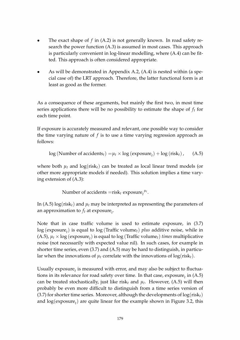
• The exact shape of f in (A.2) is not generally known. In road safety re-
search the power function (A.3) is assumed in most cases. This approach
is particularly convenient in log-linear modelling, where (A.4) can be fit-
ted. This approach is often considered appropriate.
• As will be demonstrated in Appendix A.2, (A.4) is nested within (a spe-
cial case of) the LRT approach. Therefore, the latter functional form is at
least as good as the former.
As a consequence of these arguments, but mainly the first two, in most time
series applications there will be no possibility to estimate the shape of ft for
each time point.
If exposure is accurately measured and relevant, one possible way to consider
the time varying nature of f is to use a time varying regression approach as
follows:
log (Number of accidentst) =µt × log (exposuret) + log (riskt) , (A.5)
where both µt and log(riskt) can be treated as local linear trend models (or
other more appropriate models if needed). This solution implies a time vary-
ing extension of (A.3):
Number of accidents =riskt exposuretµt .
In (A.5) log(riskt) and µt may be interpreted as representing the parameters of
an approximation to ft at exposuret.
Note that in case traffic volume is used to estimate exposure, in (3.7)
log (exposuret) is equal to log (Traffic volumet) plus additive noise, while in
(A.5), µt × log (exposuret) is equal to log (Traffic volumet) times multiplicative
noise (not necessarily with expected value nil). In such cases, for example in
shorter time series, even (3.7) and (A.5) may be hard to distinguish, in particu-
lar when the innovations of µt correlate with the innovations of log(riskt).
Usually exposuret is measured with error, and may also be subject to fluctua-
tions in its relevance for road safety over time. In that case, exposuret in (A.5)
can be treated stochastically, just like riskt and µt. However, (A.5) will then
probably be even more difficult to distinguish from a time series version of
(3.7) for shorter time series. Moreover, although the developments of log(riskt)
and log(exposuret) are quite linear for the example shown in Figure 3.2, this
179

will not always be true in practice, in which case more elaborate models are
required.
Summarising, the possibility has to be considered that the functional form
of the non-linear relation between the number of accidents and exposure as
well as the effect of other influences on this relation change over time. Unlike
cross-sectional studies where observations are obtained over a short period of
time, in time series analysis the assumption of ‘all other variables as much as
is possible held constant’ is not very realistic, and one would therefore need to
add an additional ‘relative risk due to other influences’ latent variable to the
model. This turns the reliable identification of parameters in a time-evolving
non-linear function ft into a near impossible task. In the LRT, the ‘relative risk
due to other influences’ variable is included in the already mentioned latent
risk variable. Moreover, in the LRT the development of exposure, or even traf-
fic volume itself, is allowed to influence the development of risk directly by
choosing a a suitably defined dynamic covariance matrix (see Appendix A.2).
A.2. Elimination of the b coefficient.
As already mentioned in Appendix A.1, Elvik and Vaa (2004, p 49) discussed
the non-linear relation between the number of accidents and exposure ex-
pressed in (A.3). In Lassarre (2001) accident counts are analysed for a number
of countries and the same relation is implemented in a log-linear state space
model, as follows:
log(yt) = mt + b log(vt),
mt = mt−1 + bt−1,
bt = bt−1.
(A.6)
In (A.6), yt is the number of fatalities, vt is the observed traffic volume (not the
latent exposure), mt is the level of log-risk and b is the regression coefficient for
traffic volume. Equation (A.6) is a simplified version of the model discussed
by Lassarre (2001, p.745) since stochastic components are suppressed in (A.6),
and Lassarre also considers intervention variables and autoregressive compo-
nents. Moreover, where Lassarre (2001) used the symbol η for the regression
coefficient of traffic volume, here we follow Elvik and Vaa (2004)’s use of b for
this parameter.
180
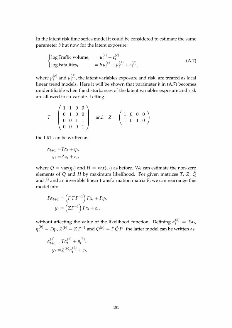
In the latent risk time series model it could be considered to estimate the same
parameter b but now for the latent exposure:
{
log Traffic volumet = µ(e)t + ε
(e)t
log Fatalitiest = b µ(e)t + µ
( f )t + ε
( f )t ,
(A.7)
where µ(e)t and µ
( f )t , the latent variables exposure and risk, are treated as local
linear trend models. Here it will be shown that parameter b in (A.7) becomes
unidentifiable when the disturbances of the latent variables exposure and risk
are allowed to co-variate. Letting
T =
1 1 0 0
0 1 0 0
0 0 1 1
0 0 0 1
and Z =
(
1 0 0 0
1 0 1 0
)
the LRT can be written as
αt+1 =Tαt + ηt,
yt =Zαt + εt,
where Q = var(ηt) and H = var(εt) as before. We can estimate the non-zero
elements of Q and H by maximum likelihood. For given matrices T, Z, Q
and H and an invertible linear transformation matrix F, we can rearrange this
model into
Fαt+1 =(
F T F−1)
Fαt + Fηt,
yt =(
ZF−1)
Fαt + εt,
without affecting the value of the likelihood function. Defining α(b)t = Fαt,
η(b)t = Fηt, Z(b) = Z F−1 and Q(b) = F Q F′, the latter model can be written as
α(b)t+1 =Tα
(b)t + η
(b)t ,
yt =Z(b)α(b)t + εt,
181

which still gives the same value of the likelihood function. We can prove the
assertion by solving the system of equations
T = F T F−1,
ZF−1 = Z(b) =
(
1 0 0 0
b 0 1 0
)
(A.8)
for F, yielding
F =
1 0 0 0
0 1 0 0
1 − b 0 1 0
0 1 − b 0 1
.
These state space representations are equivalent in terms of likelihood only if
Q(b) = F Q F′. If, for some reason, the representation of Q in the estimation
process is restricted (for instance assuming the innovations of the slopes or
levels being uncorrelated), there may be a unique and under these restrictions
optimal likelihood solution of F, and thus b may then be identifiable. Oth-
erwise, the likelihood will not improve by changing the value of b, and b is
therefore not identifiable by maximum likelihood.
One consequence of this result is that the solution based on b = 0 is also equiv-
alent in likelihood. Specifically,
Z∗ =
(
1 0 1 0
0 0 1 0
)
is also equivalent, where the component on the position of the original expo-
sure component plays the role of ‘kilometres driven per accident’.
Compared to the state space model (A.6) discussed in Lassarre (2001), the LRT
requires the estimation of four extra parameters: one for the potential covari-
ance between the observation disturbances (which should probably be present
anyway), two for the variances of the disturbances of the level and slope com-
ponents of the latent exposure, and two for the covariances of the disturbances
between the slope and level components. However, the estimation of param-
eter b is not required, and some of the just mentioned extra parameters may
not be significant. Moreover, if traffic volume is measured under observation
error, the LRT should be more appropriate.
182

A heuristic explanation of this result is that when
log (yt) =b log (exposure) + log (risk)
instead
log (yt) = log (exposure) + log (risk′)
is modelled, where
log (risk′) = log (risk) + (b − 1) log (exposure). (A.9)
Note that the derivation of the matrix F in (A.8) is based on transforming
a model based on log (yt) = log (exposure) + log (risk) to a model based
on log (yt) = b log (exposure) + log (risk′), while in (A.9) above, a model
based on log (yt) = b log (exposure) + log (risk) is transformed into log (yt) =
log (exposure) + log (risk)′, hence the difference in the coefficient 1 − b in F
and (b − 1) in (A.8). From (A.9) it can be seen that (A.8) amounts to adding
a coefficient times log (exposure) to the log (risk) component. If this opera-
tion maps one model onto another model within the same class this would
not affect the likelihood. If log (exposure) is assumed to be a local linear
trend model and log (risk) a local level model this would not be the case, as
log (risk) + (b − 1) log (exposure) would be a local linear trend model. Also,
if the innovations of log (exposure) and log (risk) are uncorrelated, the inno-
vations of log (exposure) and log (risk) + (b − 1) log (exposure) likely are cor-
related. If the model class assumes the innovations to be uncorrelated, the op-
eration (A.8) would not map the model onto a model within the same model
class. Assumptions of non-Gaussian innovation distributions may also result
in a mapping onto a model not within the same model class, and thus result in
an identifiable b.
A.3. Consequences of large dynamic prediction error for ex-
planatory variables
The modelling strategy introduced in this thesis suggests to include explan-
atory variables in the state when their observation or their effect on the road
safety system may be subject to error. In its simplest form this means that
one latent variable is added to the model for each such explanatory variable,
now to be called a latent explanatory variable. However, not all explanatory
variables necessarily have a well specified dynamic relation. More generally,
the dynamic prediction may be subject to large random error. This section
183
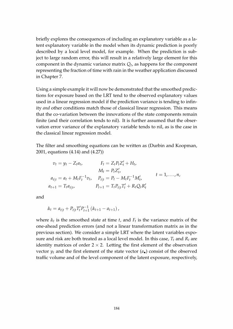
briefly explores the consequences of including an explanatory variable as a la-
tent explanatory variable in the model when its dynamic prediction is poorly
described by a local level model, for example. When the prediction is sub-
ject to large random error, this will result in a relatively large element for this
component in the dynamic variance matrix Qt, as happens for the component
representing the fraction of time with rain in the weather application discussed
in Chapter 7.
Using a simple example it will now be demonstrated that the smoothed predic-
tions for exposure based on the LRT tend to the observed explanatory values
used in a linear regression model if the prediction variance is tending to infin-
ity and other conditions match those of classical linear regression. This means
that the co-variation between the innovations of the state components remain
finite (and their correlation tends to nil). It is further assumed that the obser-
vation error variance of the explanatory variable tends to nil, as is the case in
the classical linear regression model.
The filter and smoothing equations can be written as (Durbin and Koopman,
2001, equations (4.14) and (4.27))
vt = yt − Ztat, Ft = ZtPtZ′t + Ht,
Mt = PtZ′t,
at|t = at + MtF−1t vt, Pt|t = Pt − MtF
−1t M′
t,
at+1 = Ttat|t, Pt+1 = TtPt|tT′t + RtQtR
′t
t = 1, . . . , n,
and
αt = at|t + Pt|tT′t P−1
t+1 (αt+1 − at+1) ,
where αt is the smoothed state at time t, and Ft is the variance matrix of the
one-ahead prediction errors (and not a linear transformation matrix as in the
previous section). We consider a simple LRT where the latent variables expo-
sure and risk are both treated as a local level model. In this case, Tt and Rt are
identity matrices of order 2 × 2. Letting the first element of the observation
vector yt and the first element of the state vector (a•) consist of the observed
traffic volume and of the level component of the latent exposure, respectively,
184

we have that:
Zt =
(
1 0
1 1
)
, Qt =
(
q11 q12
q12 q22
)
,
Ht =
(
h11 h12
h12 h22
)
, Pt−1|t−1 =
(
p11 p12
p12 p22
)
,
Pt =
(
p11 + q11 p12 + q12
p12 + q12 p22 + q22
)
.
In classical linear regression the elements h11 and h12 of the observation error
variance matrix Ht are assumed to be nil. For the situation where q11 → ∞ and
h11 = h12 = 0 it will be demonstrated that the first element of at|t tends to the
first element of yt (i.e., the observed traffic volume), as in that case Pt|tT′t P−1
t+1
and Pt|t both tend to a matrix with only one non-zero element:
(
0 0
0 ∗
)
.
We start by noting that Ft and MtF−1t (where h11 = h12 = 0) can now be written
as:
Ft =
(
p11 + q11 p11 + p12 + q11 + q12
p11 + p12 + q11 + q12 h22 + p11 + 2p12 + p22 + q11 + 2q12 + q22
)
,
and
[
MtF−1t
]
h11=0h12=0
=
1 0(p11+q11)(p22+q22)−(p12+q12)(h22+p12+q12)
(p12+q12)2−(p11+q11)(h22+p22+q22)
(p12+q12)2−(p11+q11)(p22+q22)
(p12+q12)2−(p11+q11)(h22+p22+q22)
.
Substitution of
A :=
[
limq11→∞
MtF−1t
]
h11=0h12=0
=
(
1 0
− p22+q22h22+p22+q22
p22+q22h22+p22+q22
)
,
185

and
B :=
[
limq11→∞
MtF−1t Zt
]
h11=0h12=0
=
(
1 0
0p22+q22
h22+p22+q22
)
,
in at|t = at + MtF−1t vt yields
at|t = (I − B)at + Ayt,
since vt = yt − Ztat. It follows that
at|t =
(
yt1h22a2−(p22+q22)(yt1−yt2)
h22+p22+q22
)
.
Similarly, it can be proven that
Pt|t =
(
0 0
0h22(p22+q22)h22+p22+q22
)
,
and
Pt|tT′t P−1
t+1 →(
0 0
0h22(p22+q22)
q22(p22+q22)+h22(p22+2q22)
)
.
Therefore in this situation only the second element of the state vector is up-
dated in the smoothing equation
αt = at|t + Pt|tT′t P−1
t+1 (αt+1 − at+1) .
This again means that the smoothed level of the latent exposure is equal to
the filtered level of the latent exposure, which in turn is equal to the observed
value for traffic volume.
Concluding, the more the LRT is unable to capture the dynamic structure of
a latent explanatory variable like exposure (as indicated by a very large value
of its dynamic variance), the more the latent explanatory exposure tends to
become equal to the observed traffic volume. The same applies to any other
explanatory variable that is included in the state of the model.
186

Appendix B. The covariance structure of accident re-
lated outcomes
Here it is shown how to derive an expression for the variance-covariance ma-
trix of the number of (injury) accidents and victims. It is assumed that a basic
simplification can be used: the number of victims per accident is equally dis-
tributed with finite variance for all accidents, although it may be possible to
relax this assumption. No further assumptions on the shape of the distribu-
tion of the accident outcomes are made. The derivation extends the result in
(Feller, 1968 page 286).
B.1. The expected value and variance of the number of vic-
tims
First define N as the number of accidents in a certain period of time. N is
assumed to be Poisson distributed with parameter λ.
Let the stochastic variables Vi (i = 1, . . . , N) denote the number of victims in
accident i. The Vi are assumed to be independently identically distributed.
The distribution of the Vi has characteristic function φ(t) and expected value µ
and all moments are finite. The symbol vi is used to denote a realisation of the
number of victims in accident i.
Let the total number of victims be V, defined as V = ∑Ni=1 Vi, thus V is a sum
over a Poisson distributed random number (N) of accidents. Defining Φ(t) as
the characteristic function of the distribution of V, we have that
Φ(t) = E(
eitV)
= E(
E(
eitV |N))
, (B.1)
where i is the imaginary number (i2 = −1). Since
E(
eitV |N = n)
= E(
eit ∑ni=1 Vi |N = n
)
= E
(
n
∏i=1
eitVi
)
=n
∏i=1
φ(t) = φn(t) (B.2)
187
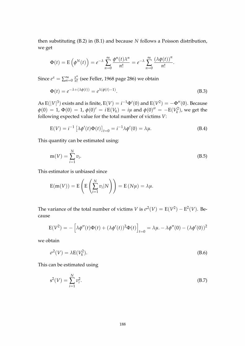
then substituting (B.2) in (B.1) and because N follows a Poisson distribution,
we get
Φ(t) = E(
φN(t))
= e−λ∞
∑n=0
φn(t)λn
n!= e−λ
∞
∑n=0
(λφ(t))n
n!.
Since ex = ∑∞n=0
xn
n! (see Feller, 1968 page 286) we obtain
Φ(t) = e−λ+(λφ(t)) = eλ(φ(t)−1). (B.3)
As E(|V|3) exists and is finite, E(V) = i−1Φ′(0) and E(V2) = −Φ′′(0). Because
φ(0) = 1, Φ(0) = 1, φ(0)′ = i E(Vk) = iµ and φ(0)′′ = −E(V2k ), we get the
following expected value for the total number of victims V:
E(V) = i−1[
λφ′(t)Φ(t)]
t=0= i−1λφ′(0) = λµ. (B.4)
This quantity can be estimated using:
m(V) =N
∑i=1
vi. (B.5)
This estimator is unbiased since
E(m(V)) = E
(
E
(
N
∑i=1
vi|N))
= E (Nµ) = λµ.
The variance of the total number of victims V is σ2(V) = E(V2) − E2(V). Be-
cause
E(V2) = −[
λφ′′(t)Φ(t) + (λφ′(t))2Φ(t)]
t=0= λµ. − λφ′′(0)− (λφ′(0))2
we obtain
σ2(V) = λE(V2k ). (B.6)
This can be estimated using
s2(V) =N
∑i=1
v2i . (B.7)
188
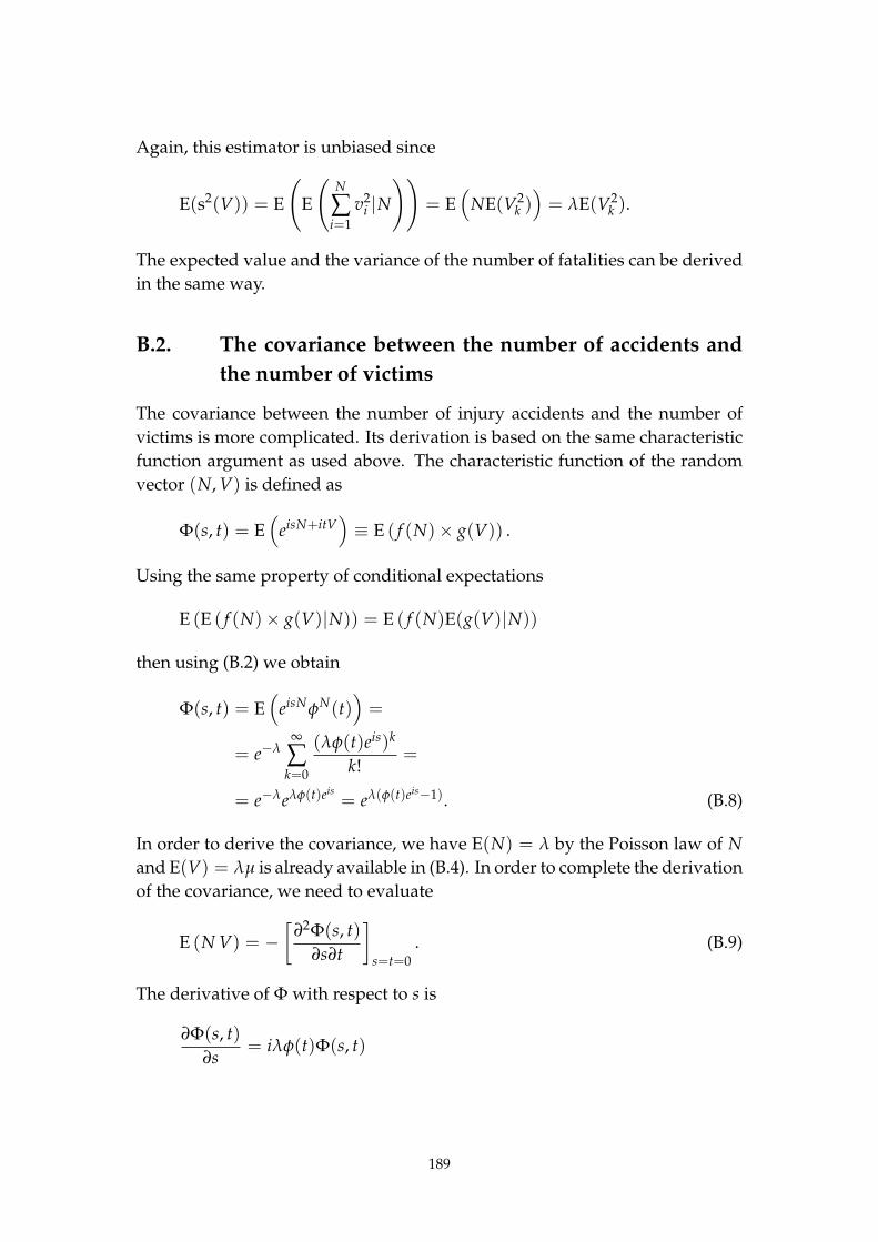
Again, this estimator is unbiased since
E(s2(V)) = E
(
E
(
N
∑i=1
v2i |N
))
= E(
NE(V2k )
)
= λE(V2k ).
The expected value and the variance of the number of fatalities can be derived
in the same way.
B.2. The covariance between the number of accidents and
the number of victims
The covariance between the number of injury accidents and the number of
victims is more complicated. Its derivation is based on the same characteristic
function argument as used above. The characteristic function of the random
vector (N, V) is defined as
Φ(s, t) = E(
eisN+itV)
≡ E ( f (N) × g(V)) .
Using the same property of conditional expectations
E (E ( f (N)× g(V)|N)) = E ( f (N)E(g(V)|N))
then using (B.2) we obtain
Φ(s, t) = E(
eisNφN(t))
=
= e−λ∞
∑k=0
(λφ(t)eis)k
k!=
= e−λeλφ(t)eis= eλ(φ(t)eis−1). (B.8)
In order to derive the covariance, we have E(N) = λ by the Poisson law of N
and E(V) = λµ is already available in (B.4). In order to complete the derivation
of the covariance, we need to evaluate
E (N V) = −[
∂2Φ(s, t)
∂s∂t
]
s=t=0
. (B.9)
The derivative of Φ with respect to s is
∂Φ(s, t)
∂s= iλφ(t)Φ(s, t)
189

and the derivative of the latter with respect to t
∂2Φ(s, t)
∂s∂t=iλφ(t)λeisφ′(t)Φ(s, t) + iλφ′(t)Φ(s, t) =
=iλΦ(s, t)φ′(t)(
φ(t)λeis + 1)
.
Because Φ(0, 0) = φ(0) = 1, and φ′(0) = iµ it follows that
[
∂2Φ(s, t)
∂s∂t
]
s=t=0
= i2λµ (λ + 1) .
Therefore
E (N V) = λµ (λ + 1) (B.10)
and thus
Cov(N, V) = λ2µ + λµ − λλµ = λµ. (B.11)
This quantity can be estimated using
s(N, V) =N
∑i=1
vi. (B.12)
Again, this estimator is unbiased because
E(s(N, V)) = E
(
E
(
N
∑i=1
vi|N))
= E (Nµ) = λµ. (B.13)
The covariance between the number of accidents and the number of fatalities
can be derived in the same manner.
B.3. The covariance between the number of victims and the
number of fatalities
Let the random variable Fi be the number of fatalities in accident i. Let F =
∑Ni=1 Fi. Define Ψ(s, t) as the characteristic function of the random vector (V, F)
and ψ(s, t) as the characteristic function of the random vector (Vi, Fi). Then,
for each i 6= j, (Vi, Fi) is independent of (Vj, Fj). However, the Vi and Fi are not
190

independent because Vi ≥ Fi a.s. Now
Ψ(s, t) = E(
eitV+isF)
= E(
E(
eitV+isF|N))
.
Following a derivation similar to (B.2) we obtain:
E(
eitV+isF|N = n)
= E(
e∑ni=1(itVi+isFi)|N = n
)
= E
(
n
∏i=1
eitVi+isFi
)
=n
∏i=1
ψ(s, t) = ψn(s, t).
Analogous to (B.8) it is found
Ψ(s, t) = E(
ψN(s, t))
= e−λ∞
∑n=0
ψn(s, t)λn
n!= e−λ
∞
∑n=0
(λψ(s, t))n
n!,
from which it follows that
Ψ(s, t) = e−λ+(λψ(s,t)) = eλ(ψ(s,t)−1).
Using the same argument as in the derivation of (B.10) we obtain
E (V F) = λ2E(Fi)E(Vi) + λE(FiVi),
and therefore
Cov(V, F) = λE(FiVi).
This can be estimated with
s(V, F) =N
∑i=1
fivi. (B.14)
Again, this estimator is unbiased.
B.4. Derivation for the logarithm of counts
B.4.1. The expected value and variance of the logarithms of number of
accidents and victims
Unfortunately, it is not possible to derive an explicit characteristic function as
simple as the one in equation (B.3) in the case of the logarithm of the number
of accidents and victims. For that reason, approximations need to be made in
order to get a useful expression for the covariance between the logarithm of
191

the number of accidents and victims. This is done using the ‘delta’ method.
The basic idea is that the logarithms of N and V are approximated by a series
expansion of order k (usually order one) about their expected values. This
results in log(N) being approximated by a polynomial in N of order k, that is,
log(N)k≈ a0 + a1 × (N − λ) + · · · + ak × (N − λ)k.
In the present case, a first order approximation about the expected value (λ) of
the number of accidents is:
log(N)1≈ log(λ) +
N − λ
λ(B.15)
where1≈ means variance of the first order approximation. Thus, the expected
value of this first order approximation is equal to log(λ): E (log(N))1≈ log(λ).
Similarly, the square of the linear approximation is
(N − λ)2
λ2+ log2(λ) + 2
(
N − λ
λ
)
log(λ).
The latter part has expected value 0, so its expected value is
σ2(N)
λ2+ log2(λ) =
1
λ+ log2(λ),
so combining we have
σ2(log(N)) ≈ σ2(N)
λ2=
1
λ, s2(log(N))≈ 1
N(B.16)
In the case of log(V), approximations are about the expected value λµ of V:
log(V)1≈ log(λµ) +
V − λµ
λµ(B.17)
For that reason E (log(V))1≈ log(λµ) and using first (B.16) and then (B.5) we
obtain
σ2 (log(V)) ≈ σ2(V)
(λµ)2=
σ2(V)
(E(V))2, s2 (log(V)) ≈ s2(V)
m(V)2. (B.18)
Results for fatalities are derived in a similar way.
192
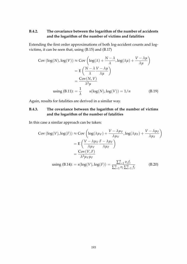
B.4.2. The covariance between the logarithm of the number of accidents
and the logarithm of the number of victims and fatalities
Extending the first order approximations of both log-accident counts and log-
victims, it can be seen that, using (B.15) and (B.17)
Cov (log(N), log(V)) ≈ Cov
(
log(λ) +N − λ
λ, log(λµ) +
V − λµ
λµ
)
= E
(
N − λ
λ
V − λµ
λµ
)
=Cov(N, V)
λ2µ
using (B.11): =1
λs(log(N), log(V)) = 1/n (B.19)
Again, results for fatalities are derived in a similar way.
B.4.3. The covariance between the logarithm of the number of victims
and the logarithm of the number of fatalities
In this case a similar approach can be taken:
Cov (log(V), log(F)) ≈ Cov
(
log(λµV) +V − λµV
λµV, log(λµF) +
V − λµF
λµF
)
= E
(
V − λµV
λµV
F − λµF
λµF
)
=Cov(V, F)
λ2µVµF
using (B.14): = s(log(V), log(F)) =∑
ni=1 vi fi
∑ni=1 vi ∑
ni=1 fi
(B.20)
193
Appendix C. Score of the Laplace approximated log-
likelihood
C.1. The derivative of at|t(ψ) with respect to a parameter ψ.
Define ξt as the vector of parameters describing the distribution of the pre-
dicted state at time t. In the Gaussian case, ξt would comprise of both at|t−1
and Pt|t−1. Also assume that the derivatives with respect to the parameter
(vector) of interest ψ of the components of ξt is available. Obviously, ξt can be
assumed a function of ψ.
Because at|t(ψ) maximises lt(α, ξt(ψ), yt, ψ), at at|t(ψ) and lt can be written as
the sum of and observation and a dynamic part:
lt(α, ξt(ψ), yt, ψ) = qt(α, yt, ψ) + rt(α, ξt(ψ), ψ), (C.1)
we have for i = 1, . . . , m ≡ dim(α):
[
∂
∂αi(qt(α, yt, ψ) + rt(α, ξt(ψ), ψ))
]
α=at|t(ψ)
= 0, ∀ψ ∈ R. (C.2)
Define the following entities:
g(t)o (α, yt, ψ) =
∂
∂αqt(α, yt, ψ), g
(t)d (α, ξt, ψ) =
∂
∂αrt(α, ξt, ψ),
H(t)o (α, yt, ψ) =
∂2
∂α∂αqt(α, yt, ψ), H
(t)d (α, ξt, ψ) =
∂2
∂α∂αrt(α, ξt, ψ),
and their derivatives with respect to ψ (further suppressing the time index t):
dgo(α, yt, ψ) =∂
∂ψgo(α, yt, ψ),
dHo(α, yt, ψ) =∂
∂ψHo(α, yt, ψ),
dgd1(α, ξt, ψ) =∂
∂ψgd(α, ξt, ψ),
dgd2(α, ξt(ψ), ψ) =∂
∂ξt(ψ)gd(α, ξt(ψ), ψ).
Because (C.2) holds, we have:
go(at|t(ψ), yt, ψ) + gd(at|t(ψ), ξt(ψ), ψ) = 0, ∀ψ.
194

Taking derivatives on both sides with respect to ψ gives:
0 ≈ δ =Ho(at|t(ψ), yt, ψ)′(
∂at|t(ψ)
∂ψ
)
+ dgo(at|t(ψ), yt, ψ)+
Hd(at|t(ψ), ξt(ψ), ψ)′(
∂at|t(ψ)
∂ψ
)
+ dgd1(at|t(ψ), ξt(ψ), ψ)+
dgd2(at|t(ψ), ξt(ψ), ψ)′(
∂ξt(ψ)
∂ψ
)
, (C.3)
as by the chain rule (Magnus and Neudecker, 1999, p. 91)
∂ f (g(ψ))
∂ψ=
(
∂ f
∂g
)
(g(ψ))′(
∂g
∂ψ
)
(ψ). (C.4)
Thus, if (C.2) holds31 we have:
∂at|t(ψ)
∂ψ= −H−1
(
dgo(at|t(ψ), yt, ψ) + dgd1(at|t(ψ), ξt(ψ), ψ) +
dgd2(at|t, ξt(ψ), ψ)′(
∂ξt(ψ)
∂ψ
)
+ δ
)
, (C.5)
where −H−1 is the ‘observed covariance matrix’ of the state.
C.2. The derivative of the Hessian with respect to a param-
eter ψ.
The Hessian Ht(α, ξt(ψ), yt, ψ) of lt(α, ξt(ψ), yt, ψ) at a = at|t(ψ) is:
Ht(ψ) = [Ho(α, yt, ψ) + Hd(α, ξt(ψ), ψ)]α=at|t(ψ) ,
thus its derivative is
∂Ht(ψ)
∂ψ=
∂
∂ψHo(at|t(ψ), yt, ψ) +
∂
∂ψHd(at|t(ψ), ξt(ψ), ψ)
=
[
∂
∂ψHo(α, yt, ψ)
]
α=at|t(ψ)
+
[
∂
∂αHo(α, yt, ψ)
]′
α=at|t(ψ)
(
∂at|t(ψ)
∂ψ
)
+
[
∂
∂ψHd(α, ξ, ψ)
]
ξ=ξt(ψ)α=at|t(ψ)
+
[
∂
∂αHd(α, ξt(ψ), ψ)
]′
α=at|t(ψ)
(
∂at|t(ψ)
∂ψ
)
+
31This is only achieved numerically, so δ ≈ 0. The algorithm should verify whether δ doesnot get too far from zero.
195

[
∂
∂ξHd(at|t(ψ), ξ, ψ)
]′
ξ=ξt(ψ)
(
∂ξt(ψ)
∂ψ
)
.
The state error covariance matrix Pt|t(ψ) is estimated by minus the inverse of
the Hessian.
C.3. The derivative of the Laplace approximated log-likeli-
hood at time t
By (7.18) the integrals of the individual terms in (7.14) can be approximated:
It (a, ξt, yt, ψ) =m
2log (2π/k)− 1
2log det (−Ht (a, ξt, yt, ψ))
+lt (a, ξt, yt, ψ) .(C.6)
Using the chain rule (C.4) we need to obtain the derivative with respect to ψ of
It(at|t(ψ), ξt(ψ), yt, ψ). Using the standard results:
∂
∂ψlog det F = trace
[
F−1 ∂
∂ψF
]
and∂
∂ψF−1 = −F−1
(
∂
∂ψF
)
F−1 (C.7)
Ignoring constant terms, we have
∂
∂ψIt
(
at|t(ψ), ξt(ψ), yt, ψ)
=
− 1
2
∂
∂ψlog det
(
−Ht
(
at|t(ψ), ξt(ψ), yt, ψ))
+∂
∂ψlt
(
at|t(ψ), ξt(ψ), yt, ψ)
,
= − 1
2trace
[
Pt|t
(
∂
∂ψHt(ψ)
)]
+
+
[
∂
∂ψqt(α, yt, ψ)
]
α=at|t(ψ)
+ g(t)0 (at|t(ψ), yt, ψ)′
(
∂at|t(ψ)
∂ψ
)
+
[
∂
∂ψrt(α, ξ, ψ)
]
ξ=ξt(ψ)α=at|t(ψ)
+ g(t)d (at|t(ψ), ξt(ψ), ψ)′
(
∂at|t(ψ)
∂ψ
)
+
[
∂
∂ξrt(at|t(ψ), ξ, ψ)
]′
α=at|t(ψ)
(
∂ξt(ψ)
∂ψ
)
.
(C.8)
196
C.4. The classical univariate Linear Gaussian case
Applying the Laplace approximated Gaussian state likelihood approach to the
classical univariate Linear Gaussian state space model, as described in (7.1)
and (7.2) yields results identical to the classical prediction error decomposition
(see Durbin and Koopman, 2001, p 138).
This is demonstrated using the univariate case, where Tt, Rt, Zt ≡ 1. Ignoring
constants, from (7.15) the log-likelihood is:
lt(α, ψ) =1
2
(
−(α − αt|t−1)
2
Pt|t−1
− (α − yt)2
Rt− log(Pt|t−1) − log(Rt)
)
.
Its derivative with respect to α is:
l′t(α, ψ) =∂
∂αlt(α, ψ) =
1
2
(
−2(α − αt|t−1)
Pt|t−1
− 2 (α − yt)
Rt
)
.
Solving the equation l′t(α, ψ) = 0 for α yields:
αt|t =αt|t−1Rt + Pt|t−1yt
Pt|t−1 + Rt,
so l′′t (α, ψ) = ∂∂α l′t(α, ψ) is:
l′′t (α, ψ) = −Pt|t−1 + Rt
Pt|t−1Rt.
Substituting α into lt(α, ψ) yields (ignoring constants):
lt(α, ψ) = −1
2log(Pt|t−1Rt) −
1
2
(
αt|t−1 − yt
)2
(Pt|t−1 + Rt)
Adding (−1/2) log det (−l′′(α, ψ)):
−1
2log
(
Pt|t−1 + Rt
Pt|t−1Rt
)
197
yields
lt(α, ψ) = −1
2log(Pt|t−1 + Rt) −
1
2
(
αt|t−1 − yt
)2
(Pt|t−1 + Rt),
which is equivalent to the prediction error decomposition (see also Harvey
(1989), or Durbin and Koopman (2001, p 138)).
C.5. Issues with respect to the use Laplace approximation
The following assumptions (univariate case) on lt(α, ψ) are necessary for the
Laplace approximation to be applicable (for fixed ψ):
1. lt(α, ψ) is real and continuous. This means that the observation density
must be positive for all possible outcomes and parameter values com-
bined.
2. the integral∫
exp lt(α, ψ)dα should converge,
3. lt(α, ψ) has an absolute maximum at α,
4. l′t(α, ψ) exists in a neighbourhood of α,
5. l′′t (α, ψ) < 0
Note that the Laplace approximation relies on a second order approximation
in α of lt(α, ψ) at α. Consequent on that, in the full Gaussian case the Laplace
approximation in (7.18) is accurate. Therefore the argument that (Huber et al.,
2004, p. 896) use to state that “the approximation improves as the number
of latent variables grows (because with more latent variables we need more
manifest variables).” can be extended to the linear Gaussian state space ap-
plications of structural time series that involve unobserved state components
like slopes and seasonal components. Such components will contribute sec-
ond order polynomial components to l(α, ψ), which should not deteriorate the
Laplace approximation.
198

Samenvatting
Tijdreeksanalyse in verkeersveiligheidsonderzoek met behulpvan state space methodologie
In dit proefschrift wordt een aantal studies gepresenteerd waarin tijdreeksana-
lyse wordt toegepast op geaggregeerde verkeersveiligheidsgegevens, waaron-
der aantallen verkeersongevallen, aantallen verkeersdoden en aantallen zwaar-
gewonden.
Veel onderzoek is en wordt verricht naar hoe de verkeersveiligheid kan wor-
den verbeterd. Daarbij wordt vaak geprobeerd verbanden te leggen tussen
veranderingen in aantallen verkeersongevallen of verkeersslachtoffers aan de
ene kant en aan de andere kant bijvoorbeeld factoren zoals expositie (een maat
voor de hoeveelheid verkeer), beleid, het rijden onder invloed van alcohol,
snelheidsgedrag en infrastructurele maatregelen. Een belangrijk doel hiervan
is op te sporen welke factoren gecontroleerd kunnen worden en een positief
effect op de verkeersveiligheid hebben, zodat langs die weg de verkeersveilig-
heid verbeterd kan worden.
Sommige van deze factoren, zoals regelgeving, wetgeving en beleid kunnen
rechtstreeks worden waargenomen: de datum van implementatie staat vast,
hoewel dat niet hoeft te gelden voor de naleving daarvan. Andere factoren
kunnen alleen in theorie rechtstreeks worden waargenomen. In de praktijk
zou hun rechtstreekse meting zeer moeilijk of zeer kostbaar zijn. Een voor-
beeld van dergelijke factoren is de hoeveelheid reizigerskilometers. In theorie
zou voor ieder individu iedere dag de hoeveelheid reizigerskilometers kunnen
worden vastgesteld. In de praktijk wordt dit gegeven met behulp van enquetes
geschat, hetgeen ten koste gaat van de nauwkeurigheid. Een ander voorbeeld
is het percentage bestuurders dat onder invloed van alcohol aan het verkeer
deelneemt. Dit wordt geschat met behulp van steekproefsgewijze alcoholcon-
troles. Tenslotte is een aantal factoren nog moeilijker waar te nemen zoals de
ervaring van bestuurders. Dergelijke verschillen in waarneming hebben hun
weerslag op de verschillen in nauwkeurigheid van de gegevens. Als onder
gebruikte gegevens (grote) verschillen in nauwkeurigheid voorkomen kan dat
statistische analyse nadelig beınvloeden als dat genegeerd wordt.
Een andere complicerende factor voor (tijdreeks)analyse in verkeersveiligheids-
onderzoek is dat er geen unieke maat voor de verkeersveiligheid beschikbaar
199

is. Meestal wordt verkeersveiligheid gemeten in termen van het aantal onge-
vallen of het aantal slachtoffers. Hoewel in de praktijk de situatie gecompli-
ceerder ligt, kan worden gesteld dat sommige maatregelen voor de verkeers-
veiligheid vooral van invloed zullen zijn op het ontstaan van ongevallen, en
andere maatregelen vooral op de afloop ervan (maar zo eenvoudig ligt het
niet). Wanneer een onderzoek wordt uitgevoerd naar het effect van een maat-
regel die het ontstaan van ongevallen zou moeten beınvloeden, zou de ont-
wikkeling van het aantal van een relevant type ongevallen moeten worden
bestudeerd. Aan de andere kant, als het effect van een maatregel wordt on-
derzocht die in hoofdzaak gevolgen zou hebben voor de ernst van ongevallen,
zou de ontwikkeling van het aantal slachtoffers kunnen worden bestudeerd.
De voorkeur heeft een analyse uit te voeren op zowel de ontwikkeling van
het aantal slachtoffers van een type waarop de maatregel van invloed geacht
wordt alsook, ter vergelijking, de ontwikkeling van het aantal slachtoffers van
een type waarvan niet wordt verwacht dat de maatregel daar invloed op heeft.
Behalve als gevolg van de maatregel moeten beide ontwikkelingen vergelijk-
baar zijn. Indien een vermindering van het aantal slachtoffers is aangetoond is
het vervolgens van belang vast te stellen dat het aantal slachtoffers is verlaagd
omdat ernst van ongevallen is afgenomen, en niet omdat het aantal ongevallen
is afgenomen. Daarnaast worden idealiter geen veranderingen gevonden in de
aantallen van het type slachtoffer dat niet geacht wordt beınvloed te worden
door de maatregel.
Het is echter niet waarschijnlijk dat in de praktijk aan beide voorwaarden
kan worden voldaan wanneer het aantal slachtoffers over een langere perio-
de wordt onderzocht. De mogelijkheid bestaat dat in de waargenomen peri-
ode andere factoren van invloed zijn geweest op de verkeersveiligheid. Het
is mogelijk dat de invloed van deze factoren op zich moeten worden gemo-
delleerd. Daarnaast hoeft het niet zo te zijn dat de invloed van deze factoren
volledig onafhankelijk van de maatregel is. Om in dergelijke gevallen een ver-
antwoorde statistische analyse uit te voeren kan het zinvol zijn een simultaan
model te specificeren dat de gezamenlijke afhankelijke variabelen, met name
ongevallen en slachtoffers omvat.
In dit proefschrift wordt een nieuwe benadering voor op verkeersveiligheid
georienteerde tijdreeksanalyse van de ontwikkelingen van geaggregeerde ver-
keersveiligheidsgegevens gepresenteerd, met als doel de mogelijkheden en be-
trouwbaarheid te verbeteren ten opzichte van gewoonlijk gebruikte alternatie-
ven. De benadering is gebaseerd op zogenaamde multivariate heteroscedasti-
sche structurele tijdreeksmodellen en vermindert veel van de problemen van
de gebruikelijke tijdreeksmodellen gebruikt voor verkeersveiligheidsanalyse,
200
en alle van de bovengenoemde problemen. De momenteel veel gebruikte mo-
dellen kunnen deze problemen slechts ten dele verminderen.
De gelijktijdige combinatie van drie fundamentele aspecten van de aanpak be-
schreven in dit proefschrift maken verbeteringen van de tijdreeks modellen in
het verkeersveiligheidsonderzoek mogelijk. Deze drie aspecten zijn:
• Het gebruik van structurele componenten. De tijdreeksmodellen zijn op-
gebouwd met behulp van interpreteerbare structurele componenten, die
in principe de expositie, het risico en eventueel de ernst representeren,
en zonodig andere invloeden representeren zoals de registratiegraad, het
percentage gebruik van autogordels, het percentage van de bestuurders
met meer dan het wettelijke maximum voor de bloed alcohol concentra-
tie, het snelheidsgedrag van bestuurders. De structurele componenten
kunnen ook seizoensgebonden trends en patronen hebben. De voorde-
len van het gebruik van interpreteerbare componenten worden duide-
lijk als een individuele component kan worden gerelateerd aan meer dan
een afhankelijke variabele. Zo zal het gordeldraagpercentage voor meer-
dere typen ongevallen hetzelfde kunnen zijn (geldt niet altijd). Boven-
dien stellen de structurele componenten in deze modellen de onderzoe-
ker in staat onderscheid te maken tussen effecten die de verkeersveilig-
heid of belangrijke onderdelen daarvan beınvloeden en effecten die hoe
we de verkeersveiligheid waarnemen beınvloeden. Hierbij kan worden
gedacht aan de afnemende volledigheid van de registratie van ongeval-
len: ze gebeuren wel, maar we zien ze niet meer. Daarnaast stelt deze
benadering de onderzoeker op een relatief transparante manier in staat
effecten van verklarende variabelen op de relevante componenten te be-
studeren in plaats van op het aantal ongevallen of slachtoffers: bijvoor-
beeld ten behoeve van onderzoeksvragen als “heeft politie toezicht effect
op het percentage autogordelgebruik, en daarmee effect op de verkeers-
veiligheid of zit het toch anders?”
• Meerdere afhankelijke variabelen: zowel aantallen ongevallen als aan-
tallen slachtoffers kunnen worden opgenomen in een model, zonodig
apart voor meerdere typen ongevallen. Verklarende variabelen kunnen
op de traditionele manier worden opgenomen. Verklarende variabelen
die met onzekerheid gemeten zijn, zoals bijvoorbeeld gegevens verkre-
gen uit steekproeven of resultaten van ander onderzoek, kunnen in een
model worden opgenomen waarbij een structurele component gebruikt
wordt als schatting van de werkelijke waarde (de waarde zonder obser-
vatiefout, hetgeen zinvol kan zijn als verondersteld kan worden dat de
201

werkelijke waarde invloed heeft op de verkeersveiligheid of andere com-
ponenten, en niet de geobserveerde waarde). Een voorbeeld is het per-
centage autogordelgebruik. Gegevens hiervoor kunnen zijn verkregen
uit relatief kleine onderzoeken, en niet noodzakelijkerwijs beschikbaar
voor alle tijdstippen. Als kan worden verondersteld dat het percentage
gebruik van de autogordel ongeveer constant is, kan een structurele com-
ponent worden gebruikt die het gemiddelde van alle waarnemingen is.
Deze structurele component kan vervolgens worden gebruikt voor alle
tijdstippen, inclusief tijdstippen waarvoor geen eigen onderzoeksresul-
taat beschikbaar is. Als niet kan worden verondersteld dat het percenta-
ge gebruik van de autogordel constant is, kan de structurele component
daarop aangepast worden, zodat nog steeds de observaties van alle tijd-
stippen bruikbaar zijn (uiteraard wordt de onzekerheid over het percen-
tage autogordelgebruik op een bepaald tijdstip dan (veel) groter).
• Niet identieke structuur van waarnemingsfouten: de nauwkeurigheid
kan varieren in de tijd. Een voorbeeld is de OVG/MON mobiliteitsen-
quete, die behoorlijk in omvang is veranderd. Een extreem voorbeeld is
het geheel ontbreken van gegevens. Niet alle enquetes of onderzoeken
worden ieder jaar uitgevoerd.
De modellen gebaseerd op de aanpak beschreven in dit proefschrift kunnen
omstandigheden hanteren waarin variabelen verschillen in nauwkeurigheid.
Bijvoorbeeld, de hoeveelheid verkeer in auto’s kan nauwkeuriger worden be-
paald dan de hoeveelheid verkeer op motorfietsen (de relatieve fout voor de
totale hoeveelheid verkeer in auto’s is ongeveer 2 tot 3% in de mobiliteitsen-
quete van 2003, terwijl de relatieve fout voor het totale verkeer van motorfiet-
sen bijna 30% is in deze mobiliteitsenquete van 2003). Het is de combinatie
van deze eigenschappen in een model en het gebruik van gedeelde structu-
rele componenten dat het model aantrekkelijk maakt voor tijdreeksanalyse in
verkeersveiligheidsonderzoek. Gezien het feit dat in verkeersveiligheidson-
derzoek over het algemeen een langere periode wordt bestudeerd, waar de
omstandigheden kunnen veranderen in de loop van de tijd, kunnen de vol-
gende praktische voordelen worden genoemd:
• Omdat verschillende afhankelijke variabelen tegelijk in samenhang kun-
nen worden geanalyseerd en het feit dat geen identieke structuur van
waarnemingsfouten wordt geeist, kunnen de modellen worden gebruikt
om rekening te houden met covariantie tussen de afhankelijke variabe-
len. Het is bekend dat het aantal slachtoffers in een periode (mede) af-
202

hankelijk is van het aantal ongevallen. Het is niet per se opvallend dat
een jaar met meer ongevallen ook meer slachtoffers heeft.
Het zou wel opvallend zijn als een jaar meer ongevallen heeft en minder
slachtoffers, of minder ongevallen en meer slachtoffers. Terwijl de abso-
lute verschillen even groot zijn (een zelfde aantal meer of minder onge-
vallen of slachtoffers), is een jaar met meer ongevallen en meer slachtof-
fers of minder ongevallen en minder slachtoffers minder onwaarschijn-
lijk dan een jaar met meer ongevallen en minder slachtoffers, of minder
ongevallen en meer slachtoffers.
Met andere woorden: als er in een jaar meer ongevallen zijn gebeurd,
hoeft dat niet opvallend te zijn. Als er in een jaar minder slachtoffers zijn
gevallen hoeft dat ook niet opvallend te zijn. Maar als in datzelfde jaar
zich meer ongevallen hebben voorgedaan terwijl er minder slachtoffers
zijn gevallen, kan dat best opvallend zijn.
Met deze afhankelijkheid moet rekening worden gehouden in statistische
toepassingen. Ook de fout in de hoeveelheid verkeer geschat op basis van
de enquetes kan samenhangen. De samenhang tussen aantallen onge-
vallen en slachtoffers is gebruikt in beide toepassingen van hoofdstuk 3.
De fout in de hoeveelheid verkeer van de enquetes wordt eveneens ge-
bruikt in de toepassingen van hoofdstuk 3, de Nederlandse toepassing
in hoofdstuk 5 en de aan verkeersveiligheid gerelateerde toepassing in
hoofdstuk 7.
• Het gebruik van structurele componenten stelt de onderzoeker in staat
een beperkte mate van verificatie van de resultaten uit te voeren. De ont-
wikkeling van structurele componenten over de tijd kan worden verge-
leken met secundaire informatie, hoewel als veel secundaire informatie
beschikbaar is, het waarschijnlijk beter is om die informatie in het model
op te nemen. Een succesvolle toepassing van zo’n verificatie is te vinden
in hoofdstuk 6, waar de vorm van de ontwikkeling van de hoeveelheid
gemotoriseerd verkeer buiten de bebouwde kom vergeleken is met een
schatting daarvan op basis van de lengte van het wegennet en de ver-
keersintensiteit.
• Structurele componenten kunnen gemeenschappelijk worden gebruikt
voor de specificatie van vele afhankelijke variabelen. In de verkeersvei-
ligheidstoepassing van hoofdstuk 7 worden weersomstandigheden (duur
van de neerslag) gemeten aan de hand van tien weerstations, gerelateerd
aan een structurele component die de gemiddelde duur van de neerslag
in Nederland voorstelt. Als het weer waargenomen door de stations on-
derling overeenkomt, zal de waarde van de structurele component nauw-
203

keurig bekend zijn. Aan de andere kant, als de weerstations een verschil-
lend weerbeeld geven, zal de waarde van de structurele component min-
der nauwkeurig bekend zijn. Op deze wijze kunnen observaties waar-
bij de gemiddelde hoeveelheid neerslag minder goed bekend is, minder
invloed hebben op het eindresultaat dan observaties waarbij de gemid-
delde hoeveelheid neerslag wel goed bekend is, zodat eventuele fouten
hopelijk minder gevolgen hebben. De mogelijkheid componenten te de-
len wordt ook gebruikt in hoofdstuk 3, waarin een structurele compo-
nent die het aantal slachtoffers per ongeval voorstelt wordt gedeeld door
de afhankelijke variabelen die “het aantal door de politie geregistreer-
de slachtoffers” en “een schatting van het werkelijke aantal slachtoffers”
voorstellen. Deze component wordt gebruikt voor het verbeteren van
de schatting van het werkelijke aantal ongevallen, die niet kan worden
afgeleid uit ziekenhuisgegevens.
• De aanpak maakt het mogelijk andere verdelingen dan de normale voor
de waarnemingsfouten in de modellen te gebruiken. Deze verdelingen
kunnen bovendien gecombineerd worden en per tijdstip verschillen. In
de verkeersveiligheidstoepassing van hoofdstuk 7 wordt een model voor
weer en verkeersveiligheid ontwikkeld met behulp van zowel meerdere
normaal verdeelde waarnemingsfouten als Poisson verdeelde afhankelij-
ke variabelen.
• De aanpak maakt het mogelijk verbanden te leggen tussen de zogenaam-
de innovaties van structurele componenten. Innovaties zijn schokken in
de ontwikkeling van de componenten. Wanneer de innovaties van twee
componenten gecorreleerd zijn, dan hebben de ontwikkelingen iets ge-
meenschappelijks. Dit is van belang wanneer structurele componenten
verschijnselen beschrijven die elkaar kunnen beınvloeden, zoals expo-
sitie en risico. Een ander voorbeeld is de ontwikkeling van de ernst van
ongevallen en ongevalsrisico. De ontwikkeling van de ernst van ongeval-
len is van invloed op het ontstaan van ongevallen die een bepaalde ernst
overstijgen. Als we in staat zijn de gemiddelde ongevalsernst zoveel te
verminderen dat er bijna geen doden in het verkeer meer te betreuren
zijn, dan zullen er ook bijna geen dodelijke ongevallen meer gebeuren.
Een zelfde effect doet zich voor ten gevolge van veranderingen in de be-
zettingsgraad van auto’s. Minder inzittenden betekent minder kans dat
er iemand zo zwaar gewond raakt dat hij of zij in het ziekenhuis moet
worden opgenomen of zelfs omkomt. Gemiddeld genomen zal het lijken
alsof er dus minder ongevallen gebeuren die zo erg zijn dat er zieken-
huisgewonden of doden vallen.
204

In de praktijk worden altijd min of meer ernstige ongevallen bestudeerd.
In dit proefschrift zijn dat dodelijke ongevallen en ongevallen met doden
en of ziekenhuisgewonden. Praktisch betekent dit dat valt te verwachten
dat met een afname van de gemiddelde ongevalsernst, ook het aantal
ongevallen zal afnemen.
Het feit dat de expositie van invloed kan zijn op risico’s wordt gebruikt in
bijna alle toepassingen in dit proefschrift, terwijl het feit dat de ernst van
ongevallen van invloed kan zijn op het ontstaan van ernstige ongevallen
wordt gebruikt in de eerste toepassing van hoofdstuk 3.
In de verkeersveiligheidstoepassingen in dit proefschrift is de expositie altijd
in een op een verhouding verondersteld met de omvang van het verkeer, ge-
meten in voertuigkilometers. Deze beperking is echter niet fundamenteel. De
aanpak kan ook worden toegepast op modellen die van een niet-lineaire relatie
uitgaan tussen expositie en voertuigkilometers, alsmede van een andere maat
voor het verkeersvolume dan voertuigkilometers. Bovendien zijn de dyna-
mische relaties gebruikt in dit proefschrift afgeleid van lokale lineaire trend-
modellen. Hoewel geleidelijke ontwikkelingen over het algemeen op bevre-
digende wijze benaderd lijken te kunnen worden door lokale lineaire trend-
modellen, hoeft dit niet altijd het geval te zijn. Met name het model voor de
ontwikkeling van de fractie van de hoeveelheid van het verkeer met neerslag
in hoofdstuk 7 zou kunnen worden verbeterd.
Voor de beschrijving van ontwikkelingen over de tijd is bij de modellen in dit
proefschrift in alle gevallen uitgegaan uit van lineaire dynamische relaties met
normaal verdeelde toevalsfluctuaties. Dit is een aanname die niet in alle ge-
vallen hoeft op te gaan, hoewel de benadering met behulp van lokaal lineaire
trendmodellen in de praktijk goed lijkt te functioneren. De effectiviteit ervan
wordt in dit proefschrift empirisch aangetoond, alsmede van de voorgestel-
de nieuwe methode van tijdreeksanalyse voor verkeersveiligheidsonderzoek.
Het is de bedoeling de ontwikkeling van de methodiek verder voort te zet-
ten in hogere dimensies en in meer gedetailleerde modellen voor de verkeers-
veiligheid. In dit proefschrift zijn de belangrijkste bijdragen van de nieuwe
aanpak gerapporteerd.
205


Dankwoord
Graag wil ik iedereen bedanken die mij geholpen heeft of met wie ik heb sa-
mengewerkt. Ik wil daarbij beginnen met mijn vrouw en kinderen, die mij de
nodige ruimte hebben gelaten. Daarna, maar niet minder, wil ik de mensen
waarmee ik direct heb samengewerkt bedanken, in het bijzonder mijn colle-
ga Jacques Commandeur, mijn co-auteur Phillip Gould, mijn promotor Siem
Jan Koopman en copromotor Kees van Montfort. Voor hun commentaar op de
verkeersveiligheidsaspecten van mijn onderzoek wil ik in het bijzonder Siem
Oppe, Fred Wegman en Shalom Hakkert bedanken.
207

Time series analysis in road safetyresearch using state space methods
Frits Bijleveld
Time series analysis in road safety research using state space m
ethods Frits Bijleveld
ISB
N: 978-90-73946-04-0VU University Amsterdam