time series analysis: 4. digital linear filtersth- · 2018-03-21 · time series analysis: 4....
TRANSCRIPT

Time Series Analysis:
4. Digital Linear Filters
P. F. Górahttp://th-www.if.uj.edu.pl/zfs/gora/
2018

Linear filters
Filtering in Fourier domain is very easy: multiply the DFT of the input by a transferfunction, which is quivalnet to taking a convolution of the input and the responsefunction of a filter.
Even though we now shall try to construct filters in the signal domain, it is conve-nient to analyse them in Fourier domain. Every possible linear filter is represen-ted by
Y (f) = H(f)X(f) . (1)
H(f) is the transfer function.
Copyright c© 2009-18 P. F. Góra 4–2

A general linear filter in the signal domain has the form
yn =q∑
k=−sαkxn−k +
p∑k=1
βkyn−k (2)
xn is a (discretized) input signal, yn is the output signal.
If s > 0, future values of the input are needed to construct the output. Such filteris non-causal . It cannot be realized on-line (or in real time).
Copyright c© 2009-18 P. F. Góra 4–3

Eq. (2):
yn =q∑
k=−sαkxn−k +
p∑k=1
βkyn−k
• If p = 0, the filter is a Finite Impulse Response filter (FIR), or a movingaverage filter. The output of such a filter dies out in a finite time after theinput has died out.
• If p > 0, the filter is Infinite Impulse Response filter (IIR), or an autoregres-sive filter. Its output can go on infinitely long after the input has died out (infact, this is a parasitic behaviour).
Copyright c© 2009-18 P. F. Góra 4–4

x(t)r(t)
y(t)
x(t)r(t)
y(t)
a FIR filter:
an IIR filter:
Copyright c© 2009-18 P. F. Góra 4–5

Causal FIR filters
yn =q∑
k=0
αkxn−k . (3)
If the input is stationary, the output also is. q is called the order of the filter .
Copyright c© 2009-18 P. F. Góra 4–6

To find the transfer function, we Fourier transform Eq. (3).
Ym =1√N
N−1∑n=0
e2πimn/Nyn =1√N
N−1∑n=0
e2πimn/Nq∑
k=0
αkxn−k
=q∑
k=0
αk1√N
N−1∑n=0
e2πimn/Nxn−k =q∑
k=0
αk1√N
N−1−k∑n′=−k
e2πim(n′+k)/Nxn′ .
(4)
Copyright c© 2009-18 P. F. Góra 4–7

By the assumption of periodicity of the input, x−l ≡ xN−l. On the other hand,exp(2πim(N−l)/N)= exp(2πim) exp(2πim(−l)/N)= exp(2πim(−l)/N).Thus
Ym =q∑
k=0
αke2πimk/N 1√
N
N−1∑n′=0
e2πimn′/Nxn′︸ ︷︷ ︸Xm
=q∑
k=0
αke2πimk/N
︸ ︷︷ ︸Hm
Xm . (5)
m/N = m/(N∆) ∆ = fm∆, where fm is them-th discrete Fourier frequency.Therefore. . .
Copyright c© 2009-18 P. F. Góra 4–8

Transfer function of a causal FIR filterhas the form
H(fm) =q∑
k=0
αk(e2πifm∆
)k= α
(e2πifm∆
), (6)
where α(z) is the following polynomial of order q
α(z) =q∑
k=0
αkzk (7)
(coefficients of the filter become coefficients of the polynomial (7)).
Usually, for the sake of simplicity, we assume that ∆ = 1, or that the sam-pling time is the time unit. Remember: With this notation, frequencies becomedimensionless and the Nyquist interval equals [−1/2,1/2].
Copyright c© 2009-18 P. F. Góra 4–9

Transfer function of a general FIR filter
The above can be easily generalized to arbitrary (non-causal) FIR filters. Thetransfer function becomes
H(fm) =q∑
k=−sαk(e2πifm∆
)k= α
(e2πifm∆
), (8)
where α(·) is now an appropriate rational function.
Copyright c© 2009-18 P. F. Góra 4–10

A simple low-pass filter
Consider a filter
yn =1
4xn−1 +
1
2xn +
1
4xn+1 . (9)
Its transfer function reads
Hc(f) =1
4e2πif +
1
2+
1
4e−2πif =
1
2+
1
2cos 2πf = cos2 πf . (10)
This transfer function is large for small frequencies and approaches zero at theends of the Nyquist interval.Copyright c© 2009-18 P. F. Góra 4–11

A simple high-pass filter
Similarly, the transfer function of the filter
yn = −1
4xn−1 +
1
2xn −
1
4xn+1 . (11)
reads
Hs(f) = −1
4e2πif +
1
2−
1
4e−2πif =
1
2−
1
2cos 2πf = sin2 πf . (12)
This transfer function is large near the ends of the Nyquist interval and nearlyzero for small frequencies.Copyright c© 2009-18 P. F. Góra 4–12

(9) is a (poor) low-pass filter.(11) is a (poor) high-pass filter.
0
0.25
0.5
0.75
1
-0.5 -0.25 0 0.25 0.5
cos2 πf
f
0
0.25
0.5
0.75
1
-0.5 -0.25 0 0.25 0.5
sin2 πf
f
Copyright c© 2009-18 P. F. Góra 4–13

The “usual” moving average
The (unweighted) moving average
yn =1
2l + 1
(xn−l + xn−l+1 + · · ·+ xn + · · ·+ xn+l−1 + xn+l
), (13)
with the transfer function
HMA(f) =1
2l + 1(1 + 2 cos 2πf + 2 cos 4πf + · · ·+ 2 cos 2lπf) (14)
is a poor low-pass filter.Copyright c© 2009-18 P. F. Góra 4–14

Transfer functions of unweighted moving averages
0
0.25
0.5
0.75
1
-0.5 -0.25 0 0.25 0.5
|HM
A(f
)|
f
l=1l=2l=3l=5
Copyright c© 2009-18 P. F. Góra 4–15

An example of the usual moving average(the noise of the order of the signal)
Moving Averages
l= 0l= 1l= 5l=16
Copyright c© 2009-18 P. F. Góra 4–16

Differentiating filters
First derivative:
dg
dx
∣∣∣∣x
'1
2
(g(x)− g(x−∆)
∆+g(x+ ∆)− g(x)
∆
)=
1
2∆g(x+∆)−
1
2∆g(x−∆) (15a)
yn =1
2∆xn+1 −
1
2∆xn−1 (15b)
H(f) =i
∆sin(2πf∆) (15c)
Second derivative:
yn =1
4∆2xn+1 −
1
2∆2xn +
1
4∆2xn−1 (16a)
H(f) = −1
∆2sin(πf∆) (16b)
Copyright c© 2009-18 P. F. Góra 4–17

0 1 2 3 4 5 6 7 8
A s
igna
l
t
0 1 2 3 4 5 6 7 8
The
der
ivat
ive
t
Copyright c© 2009-18 P. F. Góra 4–18

Phase of the transfer function
In Fourier domain,
Y (f) = H(f)X(f) . (17)
H(f) = R(f)eiφ(f), R(f) > 0. The modulus of the transfer function ampli-fies/reduces contributions from the corresponding frequencies. What does thephase, φ(f), do?
Copyright c© 2009-18 P. F. Góra 4–19

The filter (9) is non-causal, but it is easy to find its causal version: we need tointroduce a time delay :
yn =1
4xn−2 +
1
2xn−1 +
1
4xn (18)
with the transfer function
H(f) = e2πif cos2 πf . (19)
This transfer function differs from that of (9) only by a phase factor. The phasefactor in (19) is responsible for the time delay!Copyright c© 2009-18 P. F. Góra 4–20

Suppose that the phase of the transfer function depends linearly on frequencies,φ(f) = af∆. Calculate the inverse transform:
yk(t) ∼∑nH(fn)X(fn)e−2πifnk∆ =
∑nR(fn)eiafn∆X(fn)e−2πifnk∆
=∑nR(fn)X(fn)e−2πifn(k−a)∆ , (20)
which corresponds to a time shift of a units (“channels”). Therefore, filters ofa linear phase introduce a uniform time shift. Filters that do not have a linearphase introduce phase differences between various Fourier components.
Copyright c© 2009-18 P. F. Góra 4–21

A phase shift can make a difference!
-1.5
-1
-0.5
0
0.5
1
1.5
0 1 2 3 4 5 6 7 8
x
sin(2πx) + 0.5sin(3πx + 0.25π)
-1.5
-1
-0.5
0
0.5
1
1.5
0 1 2 3 4 5 6 7 8
x
sin(2πx) + 0.5sin(3πx)
Copyright c© 2009-18 P. F. Góra 4–22

FIR filters design
If we have a FIR filter
yn =q∑
k=0
αkxn−k , (21)
we know that its transfer function has the form
H(fm) =q∑
k=0
αk(e2πifm∆
)k. (22)
Note that (22) equals, up to a constant, to the DFT of the filter.Copyright c© 2009-18 P. F. Góra 4–23

An inverse problem
In practice, we need to deal with an inverse problem∗: Given an
“ideal” transfer functionH(f), find the order, q, and coefficients αk
of the filter (21) such that its transfer function is as close as possible
to the “ideal” one.
∗This is a technical term!
Copyright c© 2009-18 P. F. Góra 4–24

An intuitive approach
• Take the ideal transfer function H(f).
• Calculate the inverse transform†
h(t) =
1/2∫−1/2
H(f)e−2πift df . (23)
• Discretize h(t) in as many points, as the desired order of the filter is.
This approach usually does not work, we need to take additional steps, like trun-cating the filter, and this leads to distortions of the transfer function.
†Remember that if ∆ = 1, fNyq = 1/2.
Copyright c© 2009-18 P. F. Góra 4–25

Example: A low-pass filter
The ideal transfer function reads
H(f) =
1 |f | 6 f0 < 1/2 ,
0 |f | > f0 .(24)
The transfer function in the time domain equals
h(t) =
1/2∫−1/2
H(f)e−2πift df =
f0∫−f0
e−2πift df =sin 2πf0t
πt. (25)
The amplitude of h(t) falls off very slowly, there is no natural cut-off. A sharpedge contains all Fourier components. We either introduce an arbitrary cut-off,or do something else, mostly multiplying the ideal transfer function by a windowfunction.Copyright c© 2009-18 P. F. Góra 4–26
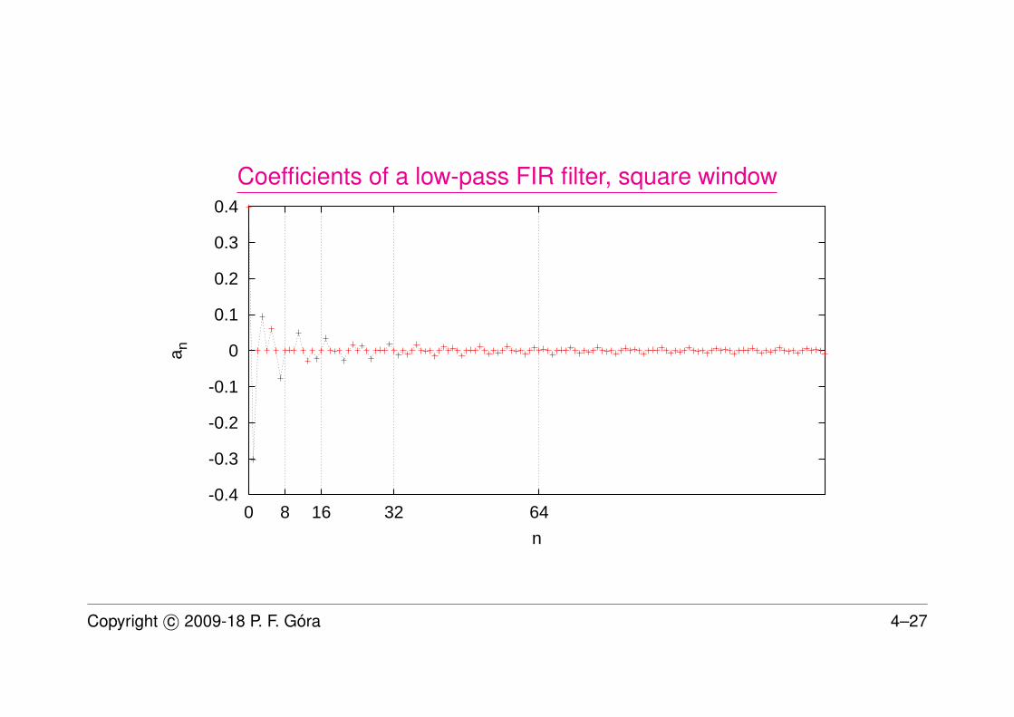
Coefficients of a low-pass FIR filter, square window
-0.4
-0.3
-0.2
-0.1
0
0.1
0.2
0.3
0.4
0 8 16 32 64
a n
n
Copyright c© 2009-18 P. F. Góra 4–27

Coefficients of a low-pass FIR filter, Hannig window
-0.4
-0.3
-0.2
-0.1
0
0.1
0.2
0.3
0.4
0.5
0 8 16 32 64
a n
n
Copyright c© 2009-18 P. F. Góra 4–28

Low-pass FIR filters discretized on a different number of points
0
0.2
0.4
0.6
0.8
1
1.2
-0.5 -0.25 0 0.25 0.5
|H(f
)|
f
n= 8
squareHanning
0
0.2
0.4
0.6
0.8
1
1.2
-0.5 -0.25 0 0.25 0.5
f
n= 16
squareHanning
0
0.2
0.4
0.6
0.8
1
1.2
-0.5 -0.25 0 0.25 0.5
f
n= 32
squareHanning
0
0.2
0.4
0.6
0.8
1
1.2
-0.5 -0.25 0 0.25 0.5
f
n= 64
squareHanning
0
0.2
0.4
0.6
0.8
1
1.2
-0.5 -0.25 0 0.25 0.5
f
n=128
squareHanning
Copyright c© 2009-18 P. F. Góra 4–29

Remarks
• Decent FIR filters require large orders.
• Window functions reduce the ripple (rapid oscillations near the edge of theband), but extend the roll-off.
• Filter design is an art. Design involves decisions on
– the ripple,
– the roll-off,
– (non)linearity of the phase,
– requirements on memory and computational complexity.
Usually you can’t optimize for all of the above simultaneously /.
• There is vast literature on filter design.
Copyright c© 2009-18 P. F. Góra 4–30

Linear IIR filters
. . . take the form
yn =q∑
k=−sαkxn−k +
p∑k=1
βkyn−k , (26)
where p > 1, xn is a (discretized) input signal, yn is the output signal. Forconvenience we discuss causal filters (s = 0) only; in fact, allowing for non-causality does not change much.
Copyright c© 2009-18 P. F. Góra 4–31

A problem
An IIR filter has a feedback loop. As a matter of principle, an IIR filter canproduce a non-zero output infinitely long after the input has ceased. Can we
avoid that?
How can we be sure that a stationary input signal produces a stationary output?
Copyright c© 2009-18 P. F. Góra 4–32

Linear difference equations
A homogeneous linear difference equation:
zn = β1zn−1 + β2zn−2 + · · ·+ βpzn−p (27)
An inhomogeneous linear difference equation:
zn = β1zn−1 + β2zn−2 + · · ·+ βpzn−p + ϕ (28)
Theorem: The general solution to an inhomogeneous difference equation equ-als a sum of the general solution to the corresponding homogeneous linear dif-ference equation and any particular solution to the inhomogeneous equation.
Stability of IIR filters is determined by the homogeneous equations.Copyright c© 2009-18 P. F. Góra 4–33

Embedding in higher dimensions
Let zn = [zn, zn−1, . . . , zn−p+1]T ∈ Rp. Then the homogeneous equation (27)can be written as
zn =
β1 β2 β3 · · · βp−1 βp1 0 0 · · · 0 00 1 0 · · · 0 0... ... ... · · · ... ...0 0 0 · · · 1 0
zn−1 . (29)
Solutions to (29) are stable if moduli of all eigenvalues are smaller that 1.
Copyright c© 2009-18 P. F. Góra 4–34

The characteristic determinant:
Wp = det
β1 − λ β2 β3 · · · βp−1 βp
1 −λ 0 · · · 0 00 1 −λ · · · 0 0... ... ... · · · ... ...0 0 0 · · · 1 −λ
= −λWp−1 + (−1)p+1βp = λ2Wp−2 + (−1)p+1βp−1λ+ (−1)p+1βp = . . .
= (−1)p+1(−λp + β1λ
p−1 + β2λp−2 + · · ·+ βp
)(30)
Copyright c© 2009-18 P. F. Góra 4–35

Stability condition of an IIR filter
An IIR filter (26) is stable if and only if roots of the equation
λp − β1λp−1 − β2λ
p−2 − · · · − βp = 0 (31)
lie inside the unit circle.
Copyright c© 2009-18 P. F. Góra 4–36

A confusion in terminology
Sometimes the above condition is formulated for the reciprocals of λ’s:
An IIR filter (26) is stable if and only if roots of the equation
1− β1u− β2u2 − · · · − βpup = 0 (32)
lie outside the unit circle.
The conditions (31), (32) are equivalent, but they should not be confused.
Copyright c© 2009-18 P. F. Góra 4–37

Example
Consider a filter
yn = β1yn−1 + xn . (33)
Its characteristic polynomial in the form (32) reads
β(z) = 1− β1z . (34)
It can be seen that if |β1| > 1, yn “explodes”, and therefore we need to have|β1| < 1, which means that the only root of (34), 1/β1, lies outside the unitinterval (and of course, outside the unit circle).Copyright c© 2009-18 P. F. Góra 4–38

IIR filter transfer function
Write (26) in the form
yn − β1yn−1 − · · · − βpyn−p = α0xn + α1xn−1 + · · ·+ αqxn−q , (35)
and Fourier transfer it. After some algebra,
H(fm) =
q∑k=0
αk(e2πifm∆
)k1−
p∑j=1
βj(e2πifm∆
)j . (36)
Note: The form of the denominator in (36) suggests that the stability condition (32) is “natural”.
Copyright c© 2009-18 P. F. Góra 4–39

IIR filters design
The trouble with IIR filters design is that one needs to avoid poles that lead toinstability. Usually, it is not easy to verify whether a pole lies inside or outsidethe unit circle. The following bilinear transform is frequently used:
z =1− iw1 + iw
or w = iz − 1
z + 1. (37)
Calculate
|z|2 =1− iw1 + iw
·1 + iw̄
1− iw̄=
1 + iw̄ − iw + |w|2
1− iw̄ + iw + |w|2=
1 + |w|2 + 2 Imw
1 + |w|2 − 2 Imw. (38)
We can see that Imw > 0 corresponds to |z|2 > 1. It is much easier to identifypoints on the upper or lower half-plane than outside or inside the unit circle.
Copyright c© 2009-18 P. F. Góra 4–40
IIR filter design procedure
• An “ideal” transfer function H(f) is given.
• Find a rational function that approximates H(f) sufficiently well. Let H(f)
be this function. It must be real and nonnegative.
• Find poles of H(f). Half of them lie in the upper half-plane, half in the lowerhalf-plane. Take a product of terms with poles from the upper half-planeonly, substitute f = i(z − 1)/(z + 1), simplify and identify the coefficients.
Copyright c© 2009-18 P. F. Góra 4–41

Example: Butterworth filter of order N
As before, we are trying to design a low-pass filter. The step function is approxi-mated by
H(f) =1
1 +(ff0
)2N , (39)
where f0 is the cut-off frequency. A filter based on (39) is called Butterworth filterof order N . Its poles lie on a circle with a radius f0, symmetrically with respectto the real axis.
(f
f0
)2N
= 1 ⇔ f = f0 exp(
2k − 1
2Niπ
), k = 0, . . . ,2N−1 . (40)
Copyright c© 2009-18 P. F. Góra 4–42

Poles of a Butterworth filter of order N = 16
Re z
Im z
f0
’good’ ploes
’bad’ ploes
Copyright c© 2009-18 P. F. Góra 4–43

N = 1 is the simplest case.
H(f) =1
1 +(ff0
)2 =i
ff0
+ i︸ ︷︷ ︸lower
·−iff0− i︸ ︷︷ ︸
upper
. (41)
We thus take−if0
f − if0=
−if0
iz−1z+1 − if0
=−f0 − f0z
z − 1− f0z − f0=
−f0 − f0z
−(1 + f0) + (1− f0)z
=
f01+f0
+ f01+f0
z
1− 1−f01+f0
z(42)
α0 = α1 = f0/(1 + f0), β1 = (1 − f0)/(1 + f0) are the coefficients of thefilter.Copyright c© 2009-18 P. F. Góra 4–44

Left: Transfer function of Butterworth filter of order 1. Middle: Transfer function of Butterworthfilter of order 4. Right: Phase of Butterworth filter of order 4.
0
0.2
0.4
0.6
0.8
1
-0.4 -0.2 0 0.2 0.4
|H(f
)|
f
0
0.2
0.4
0.6
0.8
1
-0.4 -0.2 0 0.2 0.4
|H(f
)|
f
0
π
2π
3π
4π
-0.4 -0.2 0 0.2 0.4
φ(f)
f
Copyright c© 2009-18 P. F. Góra 4–45

Most popular filters
1. Butterworth filters
• See above (39).
• The first 2N − 1 derivatives of H(f) vanish at f = 0 — the filter ismaximally flat.
• Poles lie on a circle.
• Used in audio processing.
Copyright c© 2009-18 P. F. Góra 4–46

2. Chebyshev‡ filters
• A steeper rolloff, but ripples appear.
• There are two kinds of Chebyshev filters, with ripples in thepassband :
H(f) =1
1 + [TN (f/fp)]2, (43)
and with ripples in the stopband :
H(f) =1
1 +[TN(fs/fp)TN(fs/f)
]2 . (44)
TN in the above stands for a Chebyshev polynomial of order N , fp isthe upper bound of the passband, fs > fp is the lower bound of thestopband.
‡Tschebyshef, Tchebycheff, Czebyszew
Copyright c© 2009-18 P. F. Góra 4–47

• Because of ripples, they are not used in audio processing, but it is mostexcellent if the passband contains a single “interesting” frequency (forexample, if higher harmonics are to be eliminated).
3. Elliptic filters
H(f) =1
1 + [RN (f/fp)]2, (45)
where RN is a rational function, with roots of the numerator within[−1/2,1/2], and roots of the denominator outside, with RN(1/z) =
1/RN(z). Poles of such a filter lie on an ellipsis.
4. Bessel filters, with a constant delay in the passband.
Copyright c© 2009-18 P. F. Góra 4–48

• Because a rational approximation is much better than a polynomial approxi-mation, IIR filters require significantly lower orders than FIR filters of similarperformance.
• All above filters have analog realizations, i.e. electric circuits that can filteranalog signals.
• Design of analog and digital filters is very important in electronics, telecom-munication etc. Design of good filters involves both science and art ,
Copyright c© 2009-18 P. F. Góra 4–49