RESEARCH ARTICLE

Time-resolved volumetric particle tracking velocimetryof large-scale vortex structures from the reattachment regionof a laminar separation bubble to the wake

E. Wolf • C. J. Kahler • D. R. Troolin •

C. Kykal • W. Lai

Received: 10 January 2010 / Revised: 5 August 2010 / Accepted: 1 September 2010

� Springer-Verlag 2010

Abstract The present paper presents time-resolved volu-

metric Particle Tracking Velocimetry measurements in a

water towing tank on a SD7003 airfoil, performed at a Rey-

nolds number of 60,000 and a 4� angle of attack. The SD7003

airfoil was chosen because of its long mid-chord and stable

laminar separation bubble (LSB), occurring on the suction

side of the airfoil at low Reynolds numbers. The present study

focuses on the temporal resolution of unsteady large-scale

vortex structures emitted from the LSB. In contrast to other

studies, where only the observation of the flow in the tran-

sition region was examined, the entire flow from the leading

edge to the far wake of the airfoil was investigated here.

1 Introduction

A laminar separation bubble is a typical low Reynolds

number phenomenon, which occurs on slender airfoils, as

investigated in turbine blades, sailplanes or drones. An

adverse pressure gradient (APG) causes the laminar flow to

separate from the surface and Tollmien-Schlichting (T-S)

waves develop and trigger Kelvin-Helmholtz (K-H) insta-

bilities in the shear layer above the separated region due to

inertial disturbances in the free-stream. This results in an

unsteady flow state (visible in form of Reynolds stresses)

and results in a reattachment of the apparently turbulent

shear layer (see Fig. 1). As the size of the bubble has a non-

linear dependency on a, slight changes in a may result in a

sudden enlargement of the bubble or even a separated shear

layer that never reattaches causing a broad loss of lift.

Besides the technical relevance of this phenomenon on

engine and sailplane designs, this problem is also appealing

to the fundamental point of view as a number of important

fluid mechanical effects, such as separation, transition and

turbulence, can be examined simultaneously on a small

scale.

Gaster (1966) developed a model of a 2D steady LSB

and investigated the dependency on the APG, which led

him to critical values that can cause a sudden ‘‘bursting’’ of

the bubble if exceeded. Furthermore, Horton (1968) picked

up these results and analyzed the influence of the Reynolds

number as well. He found differences between short and

long separation bubbles like the fact that short bubbles

have a much smaller and locally limited influence on the

pressure distribution than long ones. Ol et al. (2005)

compared the results measured in three different low tur-

bulence flow facilities at Reynolds number 60,000 to show

the influence of the turbulence intensity on the transition

and reattachment on the SD7003 airfoil. Figure 1 shows

the distribution of mean velocity and Reynolds stresses

measured in the Braunschweig University of Technology’s

wind tunnel at a = 4�, where one can observe the mean

locations of separation, transition and reattachment.

E. Wolf (&) � C. J. Kahler

Institute for Fluidmechanics and Aerodynamics,

University of German Armed Forces Munich,

Werner-Heisenberg-Weg 39, 85577 Neubiberg, Germany

e-mail: erik.wolf@drsnet.de

C. J. Kahler

e-mail: christian.kaehler@unibw.de

D. R. Troolin � W. Lai

TSI Incorporated, 500 Cardigan Road,

Shoreview, MN 55126, USA

e-mail: dan.troolin@tsi.com

W. Lai

e-mail: wing.lai@tsi.com

C. Kykal

TSI GmbH, Neukollner Strasse 4, 52068 Aachen, Germany

e-mail: carsten.kykal@tsi.com

123

Exp Fluids

DOI 10.1007/s00348-010-0973-2

However, as previously mentioned, the LSB is very sen-

sitive to the boundary conditions (turbulence level) and

thus highly unsteady. Pauley et al. (1990) performed

numerical investigations on the unsteady nature of the

bubble. They created an external APG and studied the

separation behavior of a two-dimensional laminar bound-

ary layer flow and found out that a high APG leads to a

periodic vortex shedding from the LSB. Furthermore, they

also suggested that Gaster’s (1966) ‘bubble-bursting’ cor-

responds to a time-averaged vortex shedding. Later, Spalart

and Strelets (2000) performed a direct numerical simula-

tion (DNS) of an LSB on a flat plate where they were able

to detect a low-frequency oscillation of the separated shear

layer known as ‘‘flapping’’ of the bubble. Due to the fact

that small disturbances in the incoming flow did not change

in the simulations, compared to experimental findings, they

suggested that K-H waves in the separated shear layer are

responsible for the transition. Similarly, Yang and Voke

(2001) discussed the K-H instability mechanism after their

large eddy simulation (LES) of flow on a flat plate. Using

the time-resolved-PIV technique, Hain and Kahler (2005)

discussed the T-S waves growing in the separated shear

layer and their relationship with the ‘‘flapping’’. Watmuff

(1999) detected the K-H wave packets by means of hot-

wire anemometry, providing 3D vortex loops at the

downstream end of the separation bubble. Zhang et al.

(2008) mapped K-H vortex structures and verified that they

are responsible for the transition in an LSB. Thereby,

they detected K-shape vortex structures rising from the

transition region. This also corresponded with 3D DNS

calculations by Alam and Sandham (2000), who had found

out that the K-vortices induce the breakdown to turbulence.

Zhang et al. (2008) were able to track these structures

being shed and propagating downstream, but not changing

their identity nor substantially decreasing in strength.

Using scanning PIV, Burgmann and Schroder (2008) and

Burgmann et al. (2007) also focused on the phenomenol-

ogy of these shed vortices. They detected the presence of

primary C-shape vortices, separating periodically from the

main recirculation region and moving further downstream.

The C-shape vortex is characterized by a distinctive back-

flow region, which was also observed by Hain and Kahler

(2005). Additionally, they depicted secondary ‘screw-

driver’ vortices with a streamwise orientation as well as

arc-like vortex structures emerging further downstream.

Burgmann and Schroder (2008) proposed a correspondence

of these vortex structures to the K-H-induced shear layer

roll-ups. Due to the three-dimensional non-stationary nat-

ure of the complex vortex structures, time-resolved inves-

tigations with a real 3D measurement system are desirable

to characterize the topology of the structures and their

development, decay and interaction. Therefore, the PTV

technique, called V3V, was used in a low turbulence water

towing tank to characterize the natural transition process in

space and time. The water towing tank was used for two

reasons: (1) to minimize its turbulence level, as the free-

stream turbulence affects the transition quite strongly and

(2) to avoid the boundary layer effects at the side-walls of

wind tunnels, which accelerate the flow over the airfoil and

thus stabilize the transition process in an unnatural way.

Fig. 1 Mean velocity (top) and

Reynolds stresses (bottom)

measured with PIV on the

SD7003 airfoil at a = 4� and

Re = 60,000 (Ol et al. 2005)

Exp Fluids

123

Besides the transition process, the influence of the tip-

vortex, which is unavoidable in towing tank experiments,

was systematically studied by changing the gap between

the tank’s bottom surface and the airfoil’s tip for two

reasons: (1) a gap flow between the airfoil and the side-wall

of the towing tank may result in a perturbation on the entire

flow field of the airfoil. Therefore, it has to be investigated

whether or not the flow is two-dimensional and the effect

of the center of the airfoil on the transition process is

negligible so that no cross-flow instability occurs. (2) As

the streamwise motion in the corner-vortex is reduced, the

free-stream flow around the airfoil is accelerated due to

continuity. This results in a larger Reynolds number and

other transition properties that are of high significance for

the present investigation. Therefore, it is essential to show

that this effect is negligible. The transition examination

shows that three-dimensional coherent vortex structures

shed near the reattachment region.

2 Experimental setup

2.1 V3V technique

Volumetric 3-Component Velocimetry (V3V) is a photo-

grammetric laser and camera-based technique licensed and

refined by TSI incorporated and based on the original

defocused digital Particle Image Velocimetry (DDPIV)

concept of Willert and Gharib (1992) and Pereira et al.

(2000) to obtain fluid velocity vectors over a relatively

large volume (12 9 12 9 10 cm3 in the current experi-

ments) at a single instant in time. A compact camera probe

consisting of three apertures (each with a 4-million-pixel

CCD array and pixel size of 7.4 microns) with three 50 mm

lenses at f#16 arranged in a triangular configuration and

separated by 17 cm was utilized to record the X, Y and

Z locations of laser-illuminated tracer particles suspended

in the fluid at two instants separated by a short time (Dt).

The camera was located at a distance of 771 mm from the

center of the measurement volume, for a maximum view-

ing angle of approximately 10�. A calibration was per-

formed by traversing a target with a known dot spacing of

5 mm through the measurement volume and capturing

images at regular intervals of 5 mm. The alignment of the

camera’s target was achieved through the use of a laser

alignment diode, mounted at the center of the camera and

oriented perpendicular to the camera face. An automated

traverse, which was used to move the target to each mea-

surement plane, was run through the full span of the

measurement volume. It was confirmed that the position of

the laser spot on the center of the target did not change

more than approximately 0.25 mm over the span of the

entire measurement volume. The position of the camera

relative to the tank was confirmed by aligning the laser

such that the reflection of the beam off the surface of the

glass was coincident with the incoming beam. The cali-

bration consists of a set of polynomial-fit equations that

relate the optical location of the calibration dot cloud to the

three sensors, through the concept of ‘‘triplets’’. The in situ

calibration corrects for image distortion (such as barrel lens

distortion) and optical aberrations (such as astigmatisms

due to viewing across the air/glass/water interface). At the

reference plane (defined as the plane where the images

from the three apertures are coincident), a single particle

lies at the same X and Y location on each camera sensor.

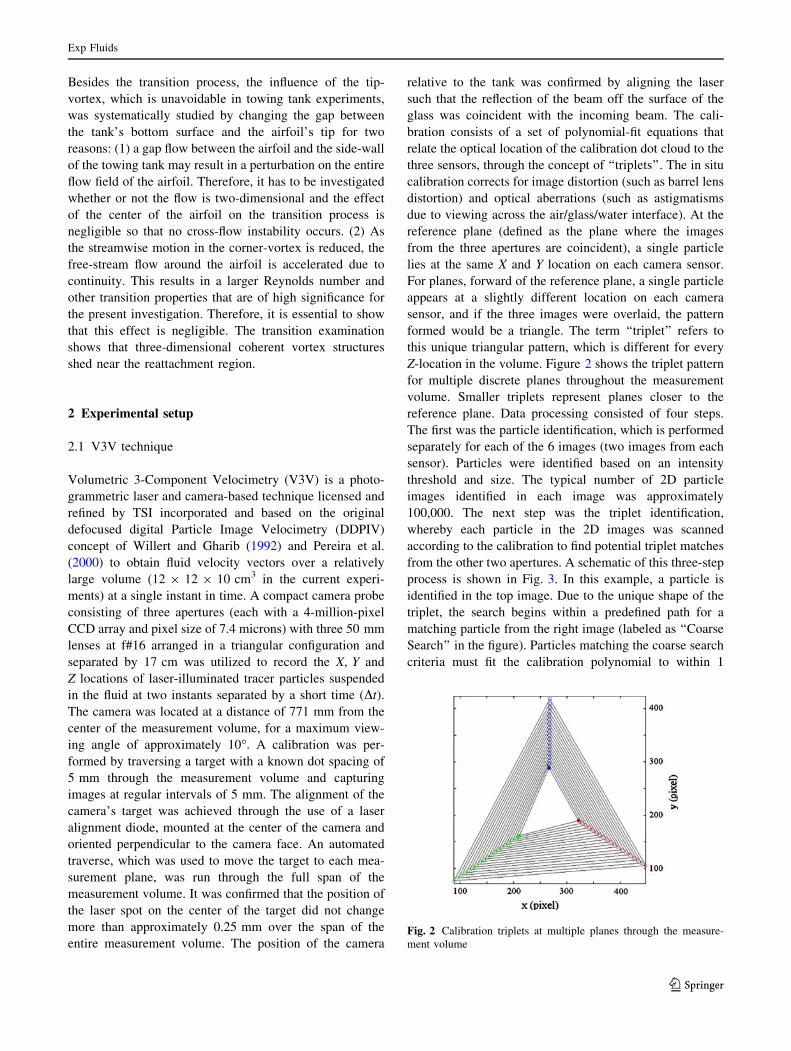
For planes, forward of the reference plane, a single particle

appears at a slightly different location on each camera

sensor, and if the three images were overlaid, the pattern

formed would be a triangle. The term ‘‘triplet’’ refers to

this unique triangular pattern, which is different for every

Z-location in the volume. Figure 2 shows the triplet pattern

for multiple discrete planes throughout the measurement

volume. Smaller triplets represent planes closer to the

reference plane. Data processing consisted of four steps.

The first was the particle identification, which is performed

separately for each of the 6 images (two images from each

sensor). Particles were identified based on an intensity

threshold and size. The typical number of 2D particle

images identified in each image was approximately

100,000. The next step was the triplet identification,

whereby each particle in the 2D images was scanned

according to the calibration to find potential triplet matches

from the other two apertures. A schematic of this three-step

process is shown in Fig. 3. In this example, a particle is

identified in the top image. Due to the unique shape of the

triplet, the search begins within a predefined path for a

matching particle from the right image (labeled as ‘‘Coarse

Search’’ in the figure). Particles matching the coarse search

criteria must fit the calibration polynomial to within 1

Fig. 2 Calibration triplets at multiple planes through the measure-

ment volume

Exp Fluids

123

pixel. Since several matches may be found, a fine search is

performed in finding a corresponding match from the left

image. Matching particles from all three images must fit

the calibration polynomial to within 0.5 pixels. These steps

were performed for every particle in the field, producing a

three-dimensional particle cloud at both instants. The third

step was the particle tracking, which utilized a three-

dimensional relaxation tracking method described in

Pereira et al. (2006). This produced a randomly spaced

vector field of typically 20,000 vectors. The data was then

interpolated onto a regular grid through Gaussian-weighted

interpolation in the fourth step.

2.2 Test facility

A water towing tank of 8.0L 9 0.9W 9 1.0H m3 was used

for the experiments. The towing device consists of a rail

car running upon the tank, precisely controlled using a

computer where acceleration and speed are continuously

adjustable in a range of 0–1.3 m/s (respectively m/s2).

Because of a minor constructional effort, the airfoil was

hung up vertically with its span aligned normal to the

tank’s bottom. Due to the nature of this setup, the complete

flow from the leading edge to the wake is observable.

However, the measurement volume at the span’s half point

should not be altered by span-wise velocities arising from

the tip-vortex’ influence, with respect to the bias of two-

dimensional flow and separation behavior. Hence, the gap

between the airfoil’s tip and the bottom of the tank had to

be minimized. For this reason, the tank bottom’s roughness

was gauged in the run-up to the measurements. Thereby,

the X-values were charted as soon as the height (Z), of the

bottom, had changed about a full millimeter. The resulting

curve is shown in Fig. 4, where Z = 0 represents the region

of highest depth. The uneven bottom of the tank is clearly

pointed out with the exaggerated axial ratio (approximately

400:1) and consequently, the vertical position of the airfoil

was adjusted using a special adapter (see Sect. 2.3). Further

direction, start- and stop-points for the towing and the locus

of test section were defined as shown in Fig. 4. With this

configuration, it was possible to accelerate the airfoil very

smoothly (0.1 m/s2) to avoid vibrations of the mounting.

Hence, having a towing speed of 0.2 m/s during the

experiments, the acceleration/deceleration phase was

finished after 0.2 m or 2.0 s. According to this, a steady

airfoil flow was guaranteed in the measurement volume of

the V3V system after 10 s of constant towing.

2.3 Construction

The constructive work included the creation of both an

airfoil and a proper adapter. With respect to the speed

range of the towing device, the chord length (c) of the

airfoil was set to 300 mm and the width to 500 mm. It was

manufactured out of massive Perspex and carefully pol-

ished afterward to avoid any surface reflections. The fully

transparent nature of the airfoil allows for the measurement

of the flow field on both sides of the airfoil simultaneously

by using the V3V technique. This was very helpful, since

the airfoil’s real position could be localized in the visual-

ization software. Obviously, the different index of refrac-

tion would introduce some parallax, but this was not

important since only transition on the suction side was of

fluid mechanical interest. Additionally, a concave form was

milled on both sides with the intention of stabilizing the

material for the cutting (especially regarding the 0.4 mm

thin trailing edge) and the polishing. The airfoil was fixed

on an aluminum plate and pinned with a shaft at x/c =

0.25, where the expected aerodynamic moments are small.

The shaft was massively constructed with a diameter of

50 mm in order to make it insensitive to any vibrations.

A frustum, serving as an indicator, was connected at the

other end of the shaft very accurately to guarantee a true

transmission of the angle of attack. The angle adjustment

happened by means of a rotary table (see Fig. 5), usually

used for optic applications. Thus, the airfoil could be

continuously rotated around the mounting axis. A simple

and precise height adjustment was realized by a three-

clamp system (see Fig. 6). Using two obstructed clamps

and one free clamp, the vertical and angle adjustments can

Fig. 3 Triplet search schematic diagram

Fig. 4 Unevenness of the towing tank’s bottom

Exp Fluids

123

be isolated from each other. With this arrangement, the

adapter is completely manageable by one person and can

be adjusted easily and precisely.

2.4 Preliminaries

For the present experiment, a frequency-doubled New

Wave YAG200-NWL dual-head pulsed Nd:YAG laser

with 200 mJ at 15 Hz was applied to illuminate neutrally

buoyant 50 lm polyamide (PA) particles. The laser was

horizontally installed underneath the test section. Similarly

to the work by Troolin and Longmire (2009), the exiting

beam was expanded to a cone using two 25 mm cylindrical

lenses, orientated perpendicular to each other. The result-

ing light cone was turned upward by a mirror (see Fig. 7).

The measurement volume in the test section was

12 9 12 9 10 cm3. Since the amount of captured particle

vectors is limited by the V3V system (see Troolin and

Longmire 2009), some light-impermeable material was

fixed under the channel to form the laser cone into a

smaller, discrete and straight volume with the objective of

increasing the spatial resolution in the region of interest

(near the airfoil surface). The dimensions of the final vector

fields were 10 9 10 9 6 cm3 with a grid spacing of 2 mm.

Furthermore, the V3V camera was arranged at right angles

with respect to the section walls and in proper height

(center of measurement volume at the span’s half). The

adapters and the airfoil were hung up vertically at the rail

car’s designated precise holding fixture so that the airfoil

could be lowered to reduce the gap down to less than 2 mm

in the test section. This is important since the tip-vortex

rising from the pressure gradient along the tip edge would

affect the flow in the span-wise direction and influence the

transition scenario. Previously, the 50 lm PA powder was

compared with 10 lm glass hollow spheres. Both of them

showed a negligible sinking speed (complete sedimentation

after 24 h), which is very important due to the fact that the

fluid is completely stagnant before each measurement.

Additional analyses have shown that both types of seeding

do not clump up, but the 10 lm tracers proved to be too

small for the tracking algorithm of the V3V system, hence

they were not used. The PA tracers were premixed to create

a homogeneous suspension. Due to the complete filling of

the tank’s volume, a frequent addition of seeding-suspen-

sion was necessary during the experiments since the

seeding disperses due to the towing of the target. Note that

the addition and suspension of PA tracer mixture took

some time to homogenize, or diffuse, until the appropriate

density for 3D particle tracking was reached in the mea-

surement volume. This can be estimated by the amount of

valid particle vectors after a fast evaluation with the sys-

tems internal software (some minutes).

3 Results

The measurements were performed at a = 4� and

Re = 60,000, which corresponds to a free-stream velocity

of u? = 0.2 m/s. As a reference, a = 8� was investigated

as well. For the final evaluation process, all visualizations

were produced with Tecplot. Hence, for a proper evalua-

tion, the data had to be transformed to the fluid mechanical

coordinate system by adding the towing speed. Moreover,

Fig. 5 Rotary table for angle adjustment

Fig. 6 Three-clamp system

Fig. 7 Test set-up with the V3V system

Exp Fluids

123

the vector fields recorded at different times were shifted

according to Dx ¼ u1=f , where f is the camera frame rate

(7.25 Hz).

3.1 Uncertainty of the arrangement

The sources of uncertainty in the V3V technique are

primarily associated with the accurate identification of

the particle locations. The sensor arrangement allows for

the determination of accurate spatial locations up to an

uncertainty of ±20 lm in X and Y, and ±80 lm in Z, as

determined by the solid motion of a plate with seeding

particles on the surface. The uncertainty in the timing

resolution was negligible, so that in the current experiment,

the uncertainty in absolute velocity, (u/u?, v/u?), was

approximately ±2.5%. But since the seeding was fre-

quently added only to the measurement volume, the

remaining volume in front of the test section showed a very

low seeding concentration in regions where the airfoil

approaches and the boundary layer develops. This is sup-

posed to be the main reason for the lack of tracers in the

boundary layer, which explains why the near-wall region

was not resolved during the experiments.

3.2 Disturbed airfoil flow

In order to examine the three-dimensional coherent vortex

structures, the free-stream flow should be two-dimensional

and a bias error due to the water surface, the starting-vortex

and the gap flow should be neglected. Since the water is at

rest and the towing speed is very low (0.2 m/s), the water

surface’s influence is negligible. But by counter-rotating to

the airfoil’s circulation, the starting-vortex has got an

immediate effect on the flow just after the initial motion of

the airfoil. The tests should consider the size, as well as the

dislocation, of the starting-vortex whose effect is strongly

related to the working principle of a towing tank. There-

fore, the airfoil was properly positioned in the measure-

ment volume with the focus on its trailing edge. The

acceleration was set to 1.0 m/s2, since it has been shown

that accelerations less than 1.0 m/s2 do not suffice for a

clear starting-vortex. This means that the airfoil is accel-

erated for only 0.2 s or 2 cm (0.06 c). Finally, the influence

due to the starting-vortex according to the Biot-Savart law

was negligible as well as the distance between the starting

point of the airfoil and the measurement section was above

2 m for the present experiments. On the other hand, the tip-

vortex may have a negative effect on the transition for two

reasons: (1) due to the span-wise flow component induced

by the gap flow, the consideration of a two-dimensional

flow might not be valid and a cross-flow instability might

be superimposed on the T-S instability and (2) due to the

deceleration of the streamwise motion in the corner-vortex,

the free-stream velocity is increased as a consequence of

continuity. This may stabilize the flow and must be

investigated as well. To study these effects, the airfoil was

lifted about 10 cm from the bottom so the measurement

volume (V3V camera) was properly positioned and the tip-

vortex could take effect. Now, the steady airfoil flow was

examined, which only has a tip-vortex in the measurement

volume, since the starting-vortex remains at the airfoil’s

starting position. As discussed, the tip-vortex would induce

a velocity in span-wise direction, which increases the total

velocity. This could heavily change the transition scenario.

In the following the investigations for a = 8� were found

to be good at presenting the tip-vortex, due to the lift

coefficient, which is at least 60% larger than at a = 4�. The

tip-vortex’ temporal-spatial development is shown in

Fig. 8. For this purpose, iso-surfaces of a negative second

Eigen value k2 (by Jeong and Hussain 1995) were plotted

and contoured with the normalized wall-parallel swirling

strength. The tip-edge is located at z = 0. As mentioned

before, all snapshots of a single measurement, recorded at

successive times, were first shifted and overlaid. Because

of this, overlapping structures might be interpreted as new

coherent ones. Nevertheless, one recognizes the tip-vortex’

history as expected. All in all, the tip-vortex’ swirling

motion causes a strong boundary layer mixing nearby.

Furthermore, span-wise velocities are induced as shown in

Fig. 9. There, the distribution of the span-wise velocity

component of five single snapshots near the airfoil is

depicted. The velocity sections are inclined about the value

of a, just as the data grid. Whereas, at t0 the flow of both

the suction and the pressure side gets distracted toward the

edge, the span-wise velocities induced by the tip-vortex are

dominant at t0 ? 0.414 s. Until t0 ? 1.242 s, the vortex-

influence moves almost completely to the suction side and

gains further momentum. At t0 ? 1.379 s purple k2-iso-

surfaces, 3D vectors along the section planes and stream-

lines were additionally inserted to mark the tip-vortex,

which has reached its maximum strength running off with

the mainstream from this point. It is important to conclude

Fig. 8 Development of a tip-vortex for a = 8� and Re = 60,000;

k2-iso-surfaces flooded with normalized stream-wise vorticity

Exp Fluids

123

that the span-wise affected area is already quite small

(z \ 0.2 c). As an additional reduction takes place for

smaller angles of attack (a = 4�) and tiny gaps (B2 mm),

the effect of the gap flow on the transition process at the

centerline can be neglected for this experiment. Afterward,

the influence becomes negligible by lowering the airfoil,

reducing the strength of the tip-vortex by decreasing the

gap and changing a to 4�. One would expect a LSB similar

to the one shown in Fig. 1 under these conditions.

3.3 Undisturbed airfoil flow

3.3.1 Vortex shedding

The incident flow near the span’s mid-point is two-dimen-

sional. As a consequence, three-dimensional coherent vor-

tex structures can be distinguished. Figure 10 shows the

instant streamwise velocity distribution. The main section

plane is at y = 0.05 c. Due to the fact that the near-wall

region was not fully resolved due to the lack of seeding (see

Sect. 3.1), the random particle vectors were additionally

plotted (black dots) to verify the credibility of the data. This

is necessary since an interpolated vector replaces every

vacancy. However, downstream of x/c = 0.7, there are

several areas of a decreased streamwise velocity magnitude

(u/u? = 0.5) also found in the literature (i.e. Burgmann

et al. 2007; Hain and Kahler 2005; Zhang et al. 2008). With

the aid of k2-iso-surfaces, the corresponding vortices could

be located as well. Their cores have an approximate size of

0.04x 9 0.04y 9 0.06z c3. As further measurements at

Re = 60,000 and a = 4� confirmed, these vortices shed

more or less in a regular chessboard pattern. In Fig. 11, the

vortices are flooded by contours of the normalized swirling

strength. Whereas the normalized span-wise vorticity xzc/

u? is uniformly negative, both xxc/u? and xyc/u? are

distributed asymmetrically on the edge regions of the vor-

tices. This underlines the three-dimensional character of

these structures and stands in interdependency with a reg-

ular distribution of sources and sinks, which is shown in

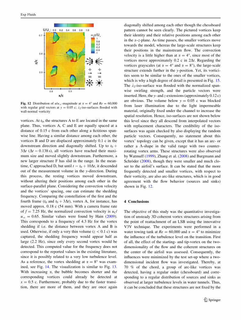
detail in Fig. 12. The snapshot displays the section-normal

view of Fig. 11 (vortices included), but this time the regular

vector field along the section plane is shown. Since the

regular vectors indicate the real instant flow behavior

(towing speed u? = 0.2 m/s2 was not yet added to the

vector field), the sources and sinks look a little unusual. It

can be stated, however, that a source is located upstream of

a vortex and a sink downstream of it. Hain et al. (2009) also

recorded the presence of sources and sinks associated with

the presence of a vortex, though in the opposite order. As a

consequence, the detected vortices seem to be different

Fig. 9 Temporal-spatial

development of the span-wise

velocity component for a = 8�and Re = 60,000

Exp Fluids

123

from the C-shape vortex by Burgmann et al. (2007) or the

ones found by Hain and Kahler (2005). Nevertheless, it

must be mentioned that their findings are not in conflict with

the present results, regarding the fact that they investigated

regions much closer to the airfoil’s surface (below y = 0.05

c). However, the vortices show similarities with the arc-like

structures first observed by Zhang et al. (2008), even though

they have to be time-resolved for a better judgment.

3.3.2 Vortex evolution

Figure 13 shows the temporal-spatial development of the

known group of vortices. For this purpose, the vortex cores

were identified with k2-iso-surfaces and flooded by the

y-magnitude to indicate their 3D position. Furthermore,

asymmetric iso-surfaces of the normalized wall-normal

vorticity were added to distinguish between individual

Fig. 10 Distribution of

u/u?-magnitude and random

particle vectors (black dots) at

a = 8� and Re = 60,000;

additionally with k2-iso-surfaces

(right)

Fig. 11 Dynamical properties

of the shed vortices; planes with

u/u?-magnitude and k2-iso-

surfaces flooded with the

different normalized vorticities

for a = 4� and Re = 60,000

Exp Fluids

123

vortices. At t0, the structures A to E are located in the same

plane. Thus, vortices A, C and E are equally spaced at a

distance of 0.15 c from each other along a fictitious span-

wise line. Having a similar distance among each other, the

vortices B and D are displaced approximately 0.1 c in the

downstream direction and diagonally shifted. Up to t0 þ3Dt (Dt ¼ 0:138 s), all vortices have reached their maxi-

mum size and moved slightly downstream. Furthermore, a

new larger structure F has slid in the range. In the mean-

time, C approached D, but until t ¼ t0 þ 10Dt, it descended

out of the measurement volume in the y-direction. During

this process, the resting vortices moved downstream,

without altering their positions among each other in the

surface-parallel plane. Considering the convection velocity

and the vortices’ spacing, one can estimate the shedding

frequency. Comparing the constellation of the first and the

fourth frame (t0 and t0 þ 3Dt), vortex A, for instance, has

moved approx. 0.18 c (54 mm). With a camera frame rate

of f = 7.25 Hz, the normalized convection velocity is uC/

u? = 0.65. Similar values were found by Hain (2009).

This corresponds to a frequency of 4.3 Hz for the vortex

shedding if i.e. the distance between vortex A and B is

used. Otherwise, if only a very thin volume (z \ 0.1 c) was

captured, the shedding frequency would appear half as

large (2.2 Hz), since only every second vortex would be

detected. This computed value for the frequency does not

correspond to the reported values in the existing literature,

since it is possibly related to a very low turbulence level.

As a reference, the vortex shedding at a = 8� was exam-

ined, see Fig. 14. The visualization is similar to Fig. 13.

With increasing a, the bubble becomes shorter and the

corresponding vortices could already be detected at

x = 0.5 c. Furthermore, probably due to the faster transi-

tion, there are more of them, and they are once again

diagonally shifted among each other though the chessboard

pattern cannot be seen clearly. The pictured vortices keep

their identity and their relative positions among each other

in the x–z-plane. As time passes, the smaller vortices move

towards the model, whereas the large-scale structures keep

their positions in the mainstream flow. The convection

velocity is a little higher than at a = 4�, since most of the

vortices move approximately 0.2 c in 2Dt. Regarding the

vortices grayscales (at a = 4� and a = 8�), the large-scale

structure extends further in the y-position. Yet, its vortici-

ties seem to be similar to the ones of the smaller vortices,

which is why a high degree of detail is presented in Fig. 15.

The k2-iso-surface was flooded with the normalized span-

wise swirling strength, and the particle vectors were

inserted. Here, the y- and z-extensions (approximately 0.12 c)

are obvious. The volume below y = 0.05 c was blocked

from laser illumination due to the light impermeable

material, originally fixed under the channel to increase the

spatial resolution. Hence, iso-surfaces are not shown below

this level since they all descend from interpolated vectors

with replacement characters. The credibility of the iso-

surfaces was again checked by also displaying the random

particle vectors. Consequently, no statement about this

vortex’ topology can be given, except that it has an arc- or

rather a K-shape in the valid range with two counter-

rotating vortex arms. These structures were also observed

by Watmuff (1999), Zhang et al. (2008) and Burgmann and

Schroder (2008), though they were smaller and much clo-

ser to the airfoil’s surface. It can be stated that the more

frequently detected and smaller vortices, with respect to

their vorticity, are also arc-like structures, which is in good

agreement with the flow behavior (sources and sinks)

shown in Fig. 12.

4 Conclusions

The objective of this study was the quantitative investiga-

tion of unsteady 3D coherent vortex structures arising from

the point of reattachment of an LSB using the innovative

V3V technique. The experiments were performed in a

water towing tank at Re = 60,000 and a = 4� to minimize

the influence of the turbulence level on the transition. First

of all, the effect of the starting- and tip-vortex on the two-

dimensionality of the flow and the coherent structures on

the center of the airfoil was assessed. Consequently, the

influences were minimized by the test set-up where a two-

dimensional incident flow was investigated. Thereby, at

70 % of the chord, a group of arc-like vortices was

detected, having a regular order (chessboard) and corre-

sponding to a regular distribution of sources and sinks as

observed at larger turbulence levels in water tunnels. Thus,

it can be concluded that these structures are not fixed by the

Fig. 12 Distribution of u/u?-magnitude at a = 4� and Re = 60,000

with regular grid vectors at y = 0.05 c; k2-iso-surfaces flooded with

wall-normal vorticity

Exp Fluids

123

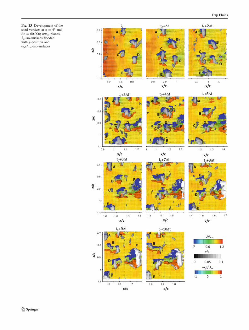
Fig. 13 Development of the

shed vortices at a = 4� and

Re = 60,000; u/u?-planes,

k2-iso-surfaces flooded

with y-position and

xyc/u?-iso-surfaces

Exp Fluids

123

free-stream-turbulence. The shed vortices’ further devel-

opment was time-resolved. Additionally, a large-scale

vortex, which extended into the illuminated volume, was

detected. In the valid range, it is arc-like and possesses two

counter-rotating vortex-arms, but the dynamics of its

structure, which extended outside of the illuminated

volume, were not resolved. Nevertheless, this study shows

that 3D K-shape coherent structures do not only exist in the

reattachment region of an LSB. They actually keep their

body structure to the far wake of the airfoil. Furthermore,

they can be regularly ordered if there is a low-turbulent

environment.

Fig. 14 Development of the

shed vortices at a = 8� and

Re = 60,000; u/u?-planes,

k2-iso-surfaces flooded

with y-position and

xyc/u?-iso-surfaces

Fig. 15 Large-scale structure at

x = 1.87 c (a = 4� and

Re = 60,000); particle vectors

flooded with u/u?-magnitude

and k2-iso-surfaces flooded with

the normalized span-wise

vorticity magnitude

Exp Fluids

123

Acknowledgments The authors like to thank Prof. Munch and

Mr. Banachowicz from the University of German Armed Forces

Munich for providing the test facility and their technical support.

References

Alam M, Sandham ND (2000) Direct numerical simulation of

‘‘Short’’ laminar separation bubbles with turbulent reattachment.

J Fluid Mech 410:1–28

Burgmann S, Dannemann J, Schroder W (2007) Time-resolved and

volumetric PIV measurements of a transitional separation bubble

on an SD7003 airfoil. Exp Fluids 44: 609–622

Burgmann S, Schroder W (2008) Investigation of the vortex induced

unsteadiness of a separation bubble via time-resolved and

scanning PIV measurements. Exp fluids 45: 675–691

Gaster M (1966) The structure and behaviour of laminar separation

bubbles. AGARD CP-4, pp 813–854

Hain R (2009) Untersuchung der Dynamik laminarer Abloseblasen

mit der zeitaufgelosten particle image velocimetry. Ph.D. Thesis,

Technical University Braunschweig

Hain R, Kahler CJ (2005) Advanced evaluation of time-resolved PIV

image sequences. In: 6th International symposium on particle

image velocimetry, Pasadena, 21–23 September

Hain R, Kahler CJ, Radespiel R (2009) Dynamics of laminar

separation bubbles at low-Reynolds number aerofoils. J Fluid

Mech 630:129–153

Horton H (1968) Laminar separation bubbles in two and three-

dimensional incompressible flow. Ph.D. Thesis, Department of

aeronautical engineering, Queen Mary College/University of

London

Jeong J, Hussain F (1995) On the identication of a vortex. J Fluid

Mech 285:69–94

Ol MV, Hanff E, McAuliffe B, Scholz U, Kahler CJ (2005)

Comparison of laminar separation bubble measurements on a

low Reynolds number airfoil in three facilities. In: 35th AIAA

fluid dynamics conference and exhibit, Toronto, 6–9 June

Pauley LL, Moin P, Reynolds WC (1990) The structure of two-

dimensional separation. J Fluid Mech 220:397–411

Pereira F, Gharib M, Dabiri D, Modarress D (2000) Defocusing

digital particle image velocimetry: a 3-component 3-dimensional

DPIV measurement technique. Application to bubbly flows. Exp

Fluids Suppl S78–S84

Pereira F, Stuer H, Graff EC, Gharib M (2006) Two-frame 3D particle

tracking. Meas Sci Technol 17:1680–1692

Spalart P, Strelets M (2000) Mechanisms of transition and heat

transfer in a separation bubble. J Fluid Mech 403:329–349

Troolin DR, Longmire EK (2009) Volumetric velocity measurements

of vortex rings from inclined exits. Exp Fluids 48:409–420

Watmuff JH (1999) Evolution of a wave packet into vortex loops in a

laminar separation bubble. J Fluid Mech 397:119–169

Willert CE, Gharib M (1992) Three-dimensional particle imaging

with a single camera. Exp Fluids 12:353–358

Yang Z, Voke PR (2001) Large-Eddy simulation of a boundary-layer

separation and transition at a change of surface curvature. J Fluid

Mech 439:305–333

Zhang W, Hain R, Kahler CJ (2008) Scanning PIV investigation of

the laminar separation bubble on a SD7003 airfoil. Exp Fluids

45:725–743

Exp Fluids

123