time petri nets: theory, tools and applications part ipopova/1-part-short.pdf · time petri nets:...
TRANSCRIPT

Time Petri Nets: Theory, Tools and Applications
Part I
Louchka Popova-Zeugmann
Humboldt-Universität zu BerlinDepartment of Computer Science
Unter den Linden 6, 10099 Berlin, Germany
ATPN 2008, Xi’an, China
Louchka Popova-Zeugmann (HU-Berlin) Time Petri nets ATPN 2008 1 / 76

Outline
1 Notions and DefinitionsPetri NetTime Petri NetTPN and Turing Machines
2 State SpaceMotivationParametric Run, Parametric StateRounding of RunsEssential StatesReachable Graph
3 Qualitative AnalysisBoundednessReachabilityLiveness
4 Quantitative AnalysisArbitrary (unbounded or bounded) TPNBounded TPN
5 Open Problems6 Appendix
Louchka Popova-Zeugmann (HU-Berlin) Time Petri nets ATPN 2008 2 / 76

Notions and Definitions Petri Net
Statics: non initialized Petri Net
initialized Petri Net
finite two-coloured weighted directed graph
initial marking: m0 = (0,1,1)
Louchka Popova-Zeugmann (HU-Berlin) Time Petri nets ATPN 2008 3 / 76

Notions and Definitions Petri Net
Statics: non initialized Petri Net
initialized Petri Net
finite two-coloured weighted directed graph
initial marking: m0 = (0,1,1)
Louchka Popova-Zeugmann (HU-Berlin) Time Petri nets ATPN 2008 3 / 76

Notions and Definitions Petri Net
Statics:
non initialized Petri Net
initialized Petri Net
finite two-coloured weighted directed graphinitial marking: m0 = (0,1,1)
Louchka Popova-Zeugmann (HU-Berlin) Time Petri nets ATPN 2008 3 / 76

Notions and Definitions Petri Net
Statics:
non initialized Petri Net
initialized Petri Net
finite two-coloured weighted directed graph
initial marking: m0 = (0,1,1)
Louchka Popova-Zeugmann (HU-Berlin) Time Petri nets ATPN 2008 3 / 76

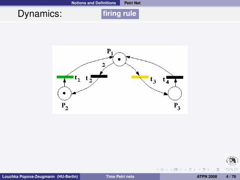
Notions and Definitions Petri Net
Dynamics: firing rule
Louchka Popova-Zeugmann (HU-Berlin) Time Petri nets ATPN 2008 4 / 76

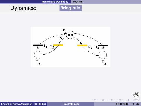
Notions and Definitions Petri Net
Dynamics: firing rule
Louchka Popova-Zeugmann (HU-Berlin) Time Petri nets ATPN 2008 4 / 76

Notions and Definitions Petri Net
Dynamics: firing rule
Louchka Popova-Zeugmann (HU-Berlin) Time Petri nets ATPN 2008 4 / 76
Notions and Definitions Petri Net
Dynamics: firing rule
Louchka Popova-Zeugmann (HU-Berlin) Time Petri nets ATPN 2008 4 / 76
Notions and Definitions Petri Net
Dynamics: firing rule
Louchka Popova-Zeugmann (HU-Berlin) Time Petri nets ATPN 2008 4 / 76

Notions and Definitions Petri Net
Petri Nets and Turing Machines
Remark:
The power of the classical Petri Nets is less (not equal) to thepower of the Turing Machines.
Assuming the opposite easily leads to a contradiction to thehalting problem.
Louchka Popova-Zeugmann (HU-Berlin) Time Petri nets ATPN 2008 5 / 76

Notions and Definitions Petri Net
Time Assignment
time dependent Petri Nets with time specification at
transitionsplacesarcstokens
time dependent Petri Nets withdeterministicstochastic
time assignment.
Louchka Popova-Zeugmann (HU-Berlin) Time Petri nets ATPN 2008 6 / 76

Notions and Definitions Petri Net
Time Assignment
time dependent Petri Nets with time specification at
transitionsplacesarcstokens
time dependent Petri Nets withdeterministicstochastic
time assignment.
Louchka Popova-Zeugmann (HU-Berlin) Time Petri nets ATPN 2008 6 / 76
Notions and Definitions Petri Net
Time Assignment
time dependent Petri Nets with time specification at
transitionsplacesarcstokens
time dependent Petri Nets withdeterministicstochastic
time assignment.
Louchka Popova-Zeugmann (HU-Berlin) Time Petri nets ATPN 2008 6 / 76
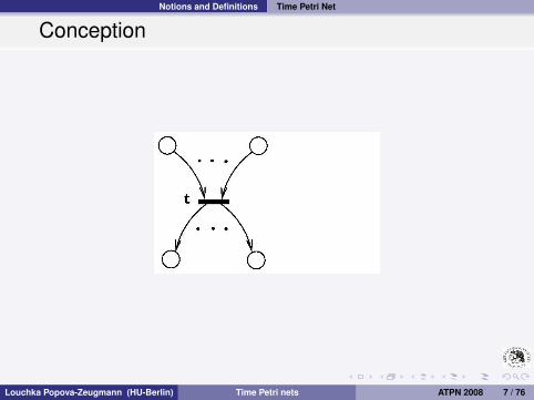
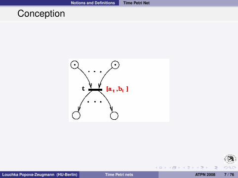
Notions and Definitions Time Petri Net
Conception
Louchka Popova-Zeugmann (HU-Berlin) Time Petri nets ATPN 2008 7 / 76

Notions and Definitions Time Petri Net
Conception
Louchka Popova-Zeugmann (HU-Berlin) Time Petri nets ATPN 2008 7 / 76
Notions and Definitions Time Petri Net
Conception
Louchka Popova-Zeugmann (HU-Berlin) Time Petri nets ATPN 2008 7 / 76

Notions and Definitions Time Petri Net
Conception
Louchka Popova-Zeugmann (HU-Berlin) Time Petri nets ATPN 2008 7 / 76

Notions and Definitions Time Petri Net
Conception
Louchka Popova-Zeugmann (HU-Berlin) Time Petri nets ATPN 2008 7 / 76

Notions and Definitions Time Petri Net
Statics:
Time
Petri Net (Skeleton)
m0 = (2,0,1)
p-marking
h0 = (],0,0,0) t-marking
h(t) is the time shown by the clock of t since the last enabling of t
Louchka Popova-Zeugmann (HU-Berlin) Time Petri nets ATPN 2008 8 / 76

Notions and Definitions Time Petri Net
Statics: Time Petri Net
(Skeleton)
m0 = (2,0,1)
p-marking
h0 = (],0,0,0) t-marking
h(t) is the time shown by the clock of t since the last enabling of t
Louchka Popova-Zeugmann (HU-Berlin) Time Petri nets ATPN 2008 8 / 76

Notions and Definitions Time Petri Net
Statics: Time Petri Net
(Skeleton)
m0 = (2,0,1)
p-markingh0 = (],0,0,0) t-marking
h(t) is the time shown by the clock of t since the last enabling of t
Louchka Popova-Zeugmann (HU-Berlin) Time Petri nets ATPN 2008 8 / 76

Notions and Definitions Time Petri Net
Statics: Time Petri Net
(Skeleton)
m0 = (2,0,1) p-marking
h0 = (],0,0,0) t-marking
h(t) is the time shown by the clock of t since the last enabling of t
Louchka Popova-Zeugmann (HU-Berlin) Time Petri nets ATPN 2008 8 / 76

Notions and Definitions Time Petri Net
Statics: Time Petri Net
(Skeleton)
m0 = (2,0,1) p-markingh0 = (],0,0,0) t-marking
h(t) is the time shown by the clock of t since the last enabling of t
Louchka Popova-Zeugmann (HU-Berlin) Time Petri nets ATPN 2008 8 / 76

Notions and Definitions Time Petri Net
Statics: Time Petri Net
(Skeleton)
m0 = (2,0,1) p-markingh0 = (],0,0,0) t-marking
h(t) is the time shown by the clock of t since the last enabling of t
Louchka Popova-Zeugmann (HU-Berlin) Time Petri nets ATPN 2008 8 / 76

Notions and Definitions Time Petri Net
State
The pair z = (m,h) is called a state in a TPN Z, iff:m is a p-marking in Z .h is a t-marking in Z.
Louchka Popova-Zeugmann (HU-Berlin) Time Petri nets ATPN 2008 9 / 76

Notions and Definitions Time Petri Net
Dynamics: firing rules
Let Z be a TPN and let z = (m,h), z ′ = (m′,h′) be two states.Z changes from state z = (m,h) into the state z ′ = (m′,h′) by:
firinga transition
/ ∖timeelapsing
Notation: z t−→ z ′ z τ−→ z ′
Louchka Popova-Zeugmann (HU-Berlin) Time Petri nets ATPN 2008 10 / 76

Notions and Definitions Time Petri Net
An example
(m0,
0]]0
)
Louchka Popova-Zeugmann (HU-Berlin) Time Petri nets ATPN 2008 11 / 76

Notions and Definitions Time Petri Net
An example
(m0,
0]]0
)1.3−→ (m1,
1.3]]
1.3
)
Louchka Popova-Zeugmann (HU-Berlin) Time Petri nets ATPN 2008 11 / 76

Notions and Definitions Time Petri Net
An example
z01.3−→ (m1,
1.3]]
1.3
)1.0−→ (m2,
2.3]]
2.3
)
Louchka Popova-Zeugmann (HU-Berlin) Time Petri nets ATPN 2008 11 / 76

Notions and Definitions Time Petri Net
An example
z01.3−→ 1.0−→ (m2,
2.3]]
2.3
)t4−→
Louchka Popova-Zeugmann (HU-Berlin) Time Petri nets ATPN 2008 11 / 76

Notions and Definitions Time Petri Net
An example
z01.3−→ 1.0−→ (m2,
2.3]]
2.3
)t4−→ (m3,
2.3]
0.0]
)
Louchka Popova-Zeugmann (HU-Berlin) Time Petri nets ATPN 2008 11 / 76

Notions and Definitions Time Petri Net
An example
z01.3−→ 1.0−→ t4−→ (m3,
2.3]
0.0]
)2.0−→ (m4,
4.3]
2.0]
)
Louchka Popova-Zeugmann (HU-Berlin) Time Petri nets ATPN 2008 11 / 76

Notions and Definitions TPN and Turing Machines
Time Petri Nets and Turing Machines
Remark:
The power of the Time Petri Nets is equal to the power of theTuring Machines.
Idea:
Simulating an arbitrary Counter Machine with a Time Petri NetCounter Machines and Turing Machines have the same power.
Louchka Popova-Zeugmann (HU-Berlin) Time Petri nets ATPN 2008 12 / 76

Notions and Definitions TPN and Turing Machines
Counter Machine
consists of
1 counters K1, . . . ,Kn,2 a numbered program, comprising 4 different commands:
start, halt, INC, DECl : command . . .
Modelling with TPN:
1 each counter Ki is modelled with a place wi
2 each program number l is modelled with a place pl
3 s. next 3 slides
Louchka Popova-Zeugmann (HU-Berlin) Time Petri nets ATPN 2008 13 / 76

Notions and Definitions TPN and Turing Machines
Modelling Counter Machines with Time Petri Nets
Notation of the Model of the numberednumbered command command as a TPN
0 : start : l
l : halt
Louchka Popova-Zeugmann (HU-Berlin) Time Petri nets ATPN 2008 14 / 76

Notions and Definitions TPN and Turing Machines
Modelling Counter Machines with Time Petri Nets
Notation of the Model of the numberednumbered command command as a TPN
l : INC(i) : r
Louchka Popova-Zeugmann (HU-Berlin) Time Petri nets ATPN 2008 15 / 76

Notions and Definitions TPN and Turing Machines
Modelling Counter Machines with Time Petri Nets
Notation of the Model of the numberednumbered command command as a TPN
l : DEC(i) : r : s
Louchka Popova-Zeugmann (HU-Berlin) Time Petri nets ATPN 2008 16 / 76
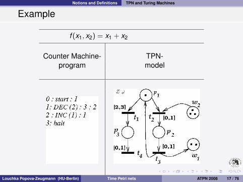
Notions and Definitions TPN and Turing Machines
Example
f (x1, x2) = x1 + x2
Counter Machine- TPN-program model
Louchka Popova-Zeugmann (HU-Berlin) Time Petri nets ATPN 2008 17 / 76

Notions and Definitions TPN and Turing Machines
A formal definition of a classical Petri Net and of a Time Petri Net canbe found in the Appendix.
Louchka Popova-Zeugmann (HU-Berlin) Time Petri nets ATPN 2008 18 / 76

Notions and Definitions TPN and Turing Machines
Definitions:
transition sequence: σ = t1 · · · tn
run: σ(τ) = τ0 t1 τ1 · · · τn−1 tn τn, τi ∈ R+0
feasible run: z0τ0−→ z∗0
t1−→ z1τ1−→ z∗1 · · ·
tn−→ znτn−→ z∗n
feasible transition sequence : σ is feasible if there ex. afeasible run σ(τ)
Louchka Popova-Zeugmann (HU-Berlin) Time Petri nets ATPN 2008 19 / 76

Notions and Definitions TPN and Turing Machines
Reachable state, Reachable marking, State space
Definitions:
z is a reachable state in Z if there ex. a feasible run σ(τ)
and z0σ(τ)−→ z
m is a reachable p-marking in Z if there ex. a reachablestate z in Z with z = (m,h)
The set of all reachable states in Z is the state space of Z( denoted: StSp(Z) ).
Louchka Popova-Zeugmann (HU-Berlin) Time Petri nets ATPN 2008 20 / 76

State Space Motivation
Qualitative Properties
static properties:
being/havinghomogenousordinaryfree choiceextended simpleconservativedeadlocks, etc.
decidable without knowledge of the state space!
dynamic properties:
being/havingboundedlivereachable marking/state, etc.
decidable, if at all (TPN are equiv. to TM!),with implicit/explicit knowledge of the state space
Louchka Popova-Zeugmann (HU-Berlin) Time Petri nets ATPN 2008 21 / 76

State Space Motivation
Qualitative Properties
static properties: being/havinghomogenousordinaryfree choiceextended simpleconservativedeadlocks, etc.
decidable without knowledge of the state space!
dynamic properties: being/havingboundedlivereachable marking/state, etc.
decidable, if at all (TPN are equiv. to TM!),with implicit/explicit knowledge of the state space
Louchka Popova-Zeugmann (HU-Berlin) Time Petri nets ATPN 2008 21 / 76

State Space Motivation
Qualitative Properties
static properties: being/havinghomogenousordinaryfree choiceextended simpleconservativedeadlocks, etc.
decidable without knowledge of the state space!dynamic properties: being/having
boundedlivereachable marking/state, etc.
decidable, if at all (TPN are equiv. to TM!),with implicit/explicit knowledge of the state space
Louchka Popova-Zeugmann (HU-Berlin) Time Petri nets ATPN 2008 21 / 76

State Space Motivation
Quantitative Properties
Each time proposition, like calculating(min/max) time length of pathpath between two states/markings with min/max time length, etc.
Decidable (if at all) with implicit/explicit knowledgeof the state space
Louchka Popova-Zeugmann (HU-Berlin) Time Petri nets ATPN 2008 22 / 76

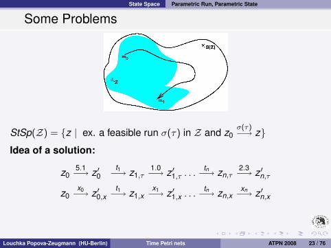
State Space Parametric Run, Parametric State
Some Problems
StSp(Z) = {z | ex. a feasible run σ(τ) in Z and z0σ(τ)−→ z}
Idea of a solution:
z05.1−→ z ′0
,τ
t1−→ z1
,τ
1.0−→ z ′1
,τ
. . .tn−→ zn
,τ
2.3−→ z ′n
,τ
τ = 5.1 1.0 . . . 2.3z0
x0−→ z ′0,xt1−→ z1,x
x1−→ z ′1,x . . .tn−→ zn,x
xn−→ z ′n,x
parametric run: σ(x) = x0 t1 x1 . . . xn−1 tn xn(+ some conditions for all xi )
Louchka Popova-Zeugmann (HU-Berlin) Time Petri nets ATPN 2008 23 / 76

State Space Parametric Run, Parametric State
Some Problems
StSp(Z) = {z | ex. a feasible run σ(τ) in Z and z0σ(τ)−→ z}
Idea of a solution:
z05.1−→ z ′0,τ
t1−→ z1,τ1.0−→ z ′1,τ . . .
tn−→ zn,τ2.3−→ z ′n,τ
τ = 5.1 1.0 . . . 2.3
z0x0−→ z ′0,x
t1−→ z1,xx1−→ z ′1,x . . .
tn−→ zn,xxn−→ z ′n,x
parametric run: σ(x) = x0 t1 x1 . . . xn−1 tn xn(+ some conditions for all xi )
Louchka Popova-Zeugmann (HU-Berlin) Time Petri nets ATPN 2008 23 / 76
State Space Parametric Run, Parametric State
Some Problems
StSp(Z) = {z | ex. a feasible run σ(τ) in Z and z0σ(τ)−→ z}
Idea of a solution:
z05.1−→ z ′0
,τ
t1−→ z1,τ1.0−→ z ′1,τ . . .
tn−→ zn,τ2.3−→ z ′n,τ
τ = 5.1 1.0 . . . 2.3
z0x0−→ z ′0,x
t1−→ z1,xx1−→ z ′1,x . . .
tn−→ zn,xxn−→ z ′n,x
parametric run: σ(x) = x0 t1 x1 . . . xn−1 tn xn(+ some conditions for all xi )
Louchka Popova-Zeugmann (HU-Berlin) Time Petri nets ATPN 2008 23 / 76

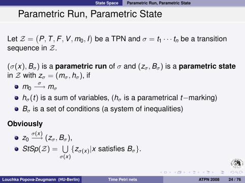
State Space Parametric Run, Parametric State
Parametric Run, Parametric State
Let Z =(P,T ,F ,V ,m0, I
)be a TPN and σ = t1 · · · tn be a transition
sequence in Z.
(σ(x),Bσ) is a parametric run of σ and (zσ,Bσ) is a parametric statein Z with zσ = (mσ,hσ), if
m0σ−→ mσ
hσ(t) is a sum of variables, (hσ is a parametrical t−marking)Bσ is a set of conditions (a system of inequalities)
Obviously
z0σ(x)−→ (zσ,Bσ),
StSp(Z) =⋃σ(x)
{zσ(x)|x satisfies Bσ}.
Louchka Popova-Zeugmann (HU-Berlin) Time Petri nets ATPN 2008 24 / 76

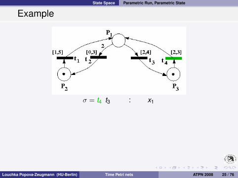
State Space Parametric Run, Parametric State
Example
σ = t4 t3
σ = t4 t3 (zσ,Bσ) =
((
011
,
x1 + x2 + x3
]]
x3
)
︸ ︷︷ ︸zσ
, {2 ≤ x1 ≤ 3, x1 + x2 ≤ 52 ≤ x2 ≤ 4, x1 + x2 + x3 ≤ 50 ≤ x3 ≤ 3
}
︸ ︷︷ ︸Bσ
).
Louchka Popova-Zeugmann (HU-Berlin) Time Petri nets ATPN 2008 25 / 76
State Space Parametric Run, Parametric State
Example
σ = t4 t3 : x1
σ = t4 t3 (zσ,Bσ) =
((
011
,
x1 + x2 + x3
]]
x3
)
︸ ︷︷ ︸zσ
, {2 ≤ x1 ≤ 3, x1 + x2 ≤ 52 ≤ x2 ≤ 4, x1 + x2 + x3 ≤ 50 ≤ x3 ≤ 3
}
︸ ︷︷ ︸Bσ
).
Louchka Popova-Zeugmann (HU-Berlin) Time Petri nets ATPN 2008 25 / 76
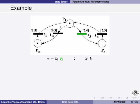
State Space Parametric Run, Parametric State
Example
σ = t4 t3 : x1 t4
σ = t4 t3 (zσ,Bσ) =
((
011
,
x1 + x2 + x3
]]
x3
)
︸ ︷︷ ︸zσ
, {2 ≤ x1 ≤ 3, x1 + x2 ≤ 52 ≤ x2 ≤ 4, x1 + x2 + x3 ≤ 50 ≤ x3 ≤ 3
}
︸ ︷︷ ︸Bσ
).
Louchka Popova-Zeugmann (HU-Berlin) Time Petri nets ATPN 2008 25 / 76

State Space Parametric Run, Parametric State
Example
σ = t4 t3 : x1 t4 x2
σ = t4 t3 (zσ,Bσ) =
((
011
,
x1 + x2 + x3
]]
x3
)
︸ ︷︷ ︸zσ
, {2 ≤ x1 ≤ 3, x1 + x2 ≤ 52 ≤ x2 ≤ 4, x1 + x2 + x3 ≤ 50 ≤ x3 ≤ 3
}
︸ ︷︷ ︸Bσ
).
Louchka Popova-Zeugmann (HU-Berlin) Time Petri nets ATPN 2008 25 / 76

State Space Parametric Run, Parametric State
Example
σ = t4 t3 : x1 t4 x2 t3 x3
σ = t4 t3 (zσ,Bσ) =
((
011
,
x1 + x2 + x3
]]
x3
)
︸ ︷︷ ︸zσ
, {2 ≤ x1 ≤ 3, x1 + x2 ≤ 52 ≤ x2 ≤ 4, x1 + x2 + x3 ≤ 50 ≤ x3 ≤ 3
}
︸ ︷︷ ︸Bσ
).
Louchka Popova-Zeugmann (HU-Berlin) Time Petri nets ATPN 2008 25 / 76

State Space Parametric Run, Parametric State
Example
σ = t4 t3
σ = t4 t3 (zσ,Bσ) =
((
011
,
x1 + x2 + x3
]]
x3
)
︸ ︷︷ ︸zσ
, {2 ≤ x1 ≤ 3, x1 + x2 ≤ 52 ≤ x2 ≤ 4, x1 + x2 + x3 ≤ 50 ≤ x3 ≤ 3
}
︸ ︷︷ ︸Bσ
).
Louchka Popova-Zeugmann (HU-Berlin) Time Petri nets ATPN 2008 25 / 76

State Space Parametric Run, Parametric State
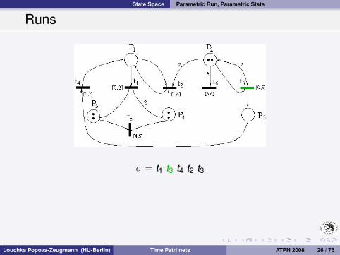
Runs
σ = t1 t3 t4 t2 t3
σ(τ) := z00.7−→ t1−→ 0.0−→ t3−→ 0.4−→ t4−→ 1.2−→ t2−→ 0.5−→ t3−→ 1.4−→ z
τ = 0.7 0.0 0.4 1.2 0.5 1.4
Louchka Popova-Zeugmann (HU-Berlin) Time Petri nets ATPN 2008 26 / 76

State Space Parametric Run, Parametric State
Runs
σ = t1 t3 t4 t2 t3
σ(τ) := z00.7−→ t1−→ 0.0−→ t3−→ 0.4−→ t4−→ 1.2−→ t2−→ 0.5−→ t3−→ 1.4−→ z
τ = 0.7 0.0 0.4 1.2 0.5 1.4
Louchka Popova-Zeugmann (HU-Berlin) Time Petri nets ATPN 2008 26 / 76
State Space Parametric Run, Parametric State
Runs
σ = t1 t3 t4 t2 t3
σ(τ) := z00.7−→ t1−→ 0.0−→ t3−→ 0.4−→ t4−→ 1.2−→ t2−→ 0.5−→ t3−→ 1.4−→ z
τ = 0.7 0.0 0.4 1.2 0.5 1.4
Louchka Popova-Zeugmann (HU-Berlin) Time Petri nets ATPN 2008 26 / 76

State Space Parametric Run, Parametric State
Runs
σ = t1 t3 t4 t2 t3
σ(τ) := z00.7−→ t1−→ 0.0−→ t3−→ 0.4−→ t4−→ 1.2−→ t2−→ 0.5−→ t3−→ 1.4−→ z
τ = 0.7 0.0 0.4 1.2 0.5 1.4
Louchka Popova-Zeugmann (HU-Berlin) Time Petri nets ATPN 2008 26 / 76

State Space Parametric Run, Parametric State
Runs
σ = t1 t3 t4 t2 t3
σ(τ) := z00.7−→ t1−→ 0.0−→ t3−→ 0.4−→ t4−→ 1.2−→ t2−→ 0.5−→ t3−→ 1.4−→ z
τ = 0.7 0.0 0.4 1.2 0.5 1.4
Louchka Popova-Zeugmann (HU-Berlin) Time Petri nets ATPN 2008 26 / 76

State Space Parametric Run, Parametric State
Runs
σ = t1 t3 t4 t2 t3
σ(τ) := z00.7−→ t1−→ 0.0−→ t3−→ 0.4−→ t4−→ 1.2−→ t2−→ 0.5−→ t3−→ 1.4−→ z
τ = 0.7 0.0 0.4 1.2 0.5 1.4
Louchka Popova-Zeugmann (HU-Berlin) Time Petri nets ATPN 2008 26 / 76

State Space Parametric Run, Parametric State
Runs
σ = t1 t3 t4 t2 t3
σ(τ) := z00.7−→ t1−→ 0.0−→ t3−→ 0.4−→ t4−→ 1.2−→ t2−→ 0.5−→ t3−→ 1.4−→ z
τ = 0.7 0.0 0.4 1.2 0.5 1.4
Louchka Popova-Zeugmann (HU-Berlin) Time Petri nets ATPN 2008 26 / 76

State Space Parametric Run, Parametric State
Runs
σ = t1 t3 t4 t2 t3
σ(τ) := z00.7−→ t1−→ 0.0−→ t3−→ 0.4−→ t4−→ 1.2−→ t2−→ 0.5−→ t3−→ 1.4−→ z
τ = 0.7 0.0 0.4 1.2 0.5 1.4
Louchka Popova-Zeugmann (HU-Berlin) Time Petri nets ATPN 2008 26 / 76

State Space Parametric Run, Parametric State
Runs
σ = t1 t3 t4 t2 t3
σ(τ) := z00.7−→ t1−→ 0.0−→ t3−→ 0.4−→ t4−→ 1.2−→ t2−→ 0.5−→ t3−→ 1.4−→ z
τ = 0.7 0.0 0.4 1.2 0.5 1.4
Louchka Popova-Zeugmann (HU-Berlin) Time Petri nets ATPN 2008 27 / 76

State Space Parametric Run, Parametric State
Example
σ = t1 t3 t4 t2 t3
mσ = (1,2,2,1,1)
Louchka Popova-Zeugmann (HU-Berlin) Time Petri nets ATPN 2008 28 / 76

State Space Parametric Run, Parametric State
Example - Continiation
hσ =
x4 + x5x5x5x5
x0 + x1 + x2 + x3 + x4 + x5]
and
Louchka Popova-Zeugmann (HU-Berlin) Time Petri nets ATPN 2008 29 / 76

State Space Parametric Run, Parametric State
Example - Continuation
Bσ = {
0 ≤ x0, x0 ≤ 2, x0 + x1 + x2 ≤ 50 ≤ x1, x2 ≤ 2, x2 + x3 ≤ 51 ≤ x2, x3 ≤ 2, x0 + x1 + x2 + x3 ≤ 51 ≤ x3, x4 ≤ 2, x0 + x1 + x2 + x3 + x4 ≤ 50 ≤ x4, x5 ≤ 2, x0 + x1 + x2 + x3 + x4 + x5 ≤ 50 ≤ x5, x0 + x1 ≤ 5 x4 + x5 ≤ 2
}.
Louchka Popova-Zeugmann (HU-Berlin) Time Petri nets ATPN 2008 30 / 76

State Space Parametric Run, Parametric State
Example - Continuation
The run σ(τ) with
z00.7−→ t1−→ 0.0−→ t3−→ 0.4−→ t4−→ 1.2−→ t2−→ 0.5−→ t3−→ 1.4−→ (mσ,
1.91.41.41.44.2]
)
is feasible.
Louchka Popova-Zeugmann (HU-Berlin) Time Petri nets ATPN 2008 31 / 76

State Space Parametric Run, Parametric State
Example - Continuation
(mσ,
1.01.01.01.04.0]
)
︸ ︷︷ ︸z0
σ(?)−→ bzc
(mσ,
1.91.41.41.44.2]
)
︸ ︷︷ ︸z0
σ(τ)−→ z
(mσ,
2.02.02.02.05.0]
)
︸ ︷︷ ︸z0
σ(?)−→ dze
Louchka Popova-Zeugmann (HU-Berlin) Time Petri nets ATPN 2008 32 / 76

State Space Parametric Run, Parametric State
Example - Continuation
(mσ,
1.01.01.01.04.0]
)
︸ ︷︷ ︸z0
σ(?)−→ bzc
(mσ,
1.91.41.41.44.2]
)
︸ ︷︷ ︸z0
σ(τ)−→ z
(mσ,
2.02.02.02.05.0]
)
︸ ︷︷ ︸z0
σ(?)−→ dze
Louchka Popova-Zeugmann (HU-Berlin) Time Petri nets ATPN 2008 32 / 76

State Space Parametric Run, Parametric State
Example - Continuation
(mσ,
1.01.01.01.04.0]
)
︸ ︷︷ ︸z0
σ(?)−→ bzc
(mσ,
1.91.41.41.44.2]
)
︸ ︷︷ ︸z0
σ(τ)−→ z
(mσ,
2.02.02.02.05.0]
)
︸ ︷︷ ︸z0
σ(?)−→ dze
Louchka Popova-Zeugmann (HU-Berlin) Time Petri nets ATPN 2008 32 / 76

State Space Parametric Run, Parametric State
Example - Continuation
The runs
σ(τ∗1 ) := z01−→ t1−→ 0−→ t3−→ 1−→ t4−→ 1−→ t2−→ 0−→ t3−→ 1−→ bzc
and
σ(τ) = z00.7−→ t1−→ 0.0−→ t3−→ 0.4−→ t4−→ 1.2−→ t2−→ 0.5−→ t3−→ 1.4−→ z
σ(τ∗2 ) := z01−→ t1−→ 0−→ t3−→ 0−→ t4−→ 2−→ t2−→ 0−→ t3−→ 2−→ dze
are also feasible in Z.
Louchka Popova-Zeugmann (HU-Berlin) Time Petri nets ATPN 2008 33 / 76

State Space Rounding of Runs
Main Property
Theorem 1:
Let Z be a TPN and σ = t1 · · · tn) be a feasible transitionsequence in Z with a feasable run σ(τ) of σ
(τ = τ0 . . . τn
)i.e.
z0τ0−→ t1−→ · · · tn−→ τn−→ zn = (mn,hn),
and all τi ∈ R+0 .
Then, there exists a further feasible run σ(τ∗), τ∗ = τ∗0 . . . τ∗n of
σ withz0
τ∗0−→ t1−→ · · · tn−→ τ∗n−→ z∗n = (m∗n,h∗n).
such that
Louchka Popova-Zeugmann (HU-Berlin) Time Petri nets ATPN 2008 34 / 76

State Space Rounding of Runs
Main Property
Theorem 1 – Continuation:
z0τ0−→ t1−→ · · · tn−→ τn−→ zn = (mn,hn), τi ∈ R+
0 .
z0τ∗0−→ t1−→ · · · tn−→ τ∗n−→ z∗n = (m∗n,h∗n)
, τ∗i ∈ N.
1 For each i ,0 ≤ i ≤ n the time τ∗i is a natural number.2 For each enabled transition t at marking mn(= m∗n) it holds:
1 h∗n(t) = bhn(t)c.
2n∑
i=1τ∗i = b
n∑i=1
τic
3 For each transition t ∈ T it holds:t is ready to fire in zn iff t is also ready to fire in bznc.
Louchka Popova-Zeugmann (HU-Berlin) Time Petri nets ATPN 2008 35 / 76

State Space Rounding of Runs
Main Property
Theorem 1 – Continuation:
z0τ0−→ t1−→ · · · tn−→ τn−→ zn = (mn,hn), τi ∈ R+
0 .
z0τ∗0−→ t1−→ · · · tn−→ τ∗n−→ z∗n = (m∗n,h∗n) , τ∗i ∈ N.
1 For each i ,0 ≤ i ≤ n the time τ∗i is a natural number.2 For each enabled transition t at marking mn(= m∗n) it holds:
1 h∗n(t) = bhn(t)c.
2n∑
i=1τ∗i = b
n∑i=1
τic
3 For each transition t ∈ T it holds:t is ready to fire in zn iff t is also ready to fire in bznc.
Louchka Popova-Zeugmann (HU-Berlin) Time Petri nets ATPN 2008 35 / 76

State Space Rounding of Runs
Main Property
Theorem 2:
Let Z be a TPN and σ = t1 · · · tn) be a feasible transitionsequence in Z, with feasable run σ(τ) of σ
(τ = τ0 . . . τn
)i.e.
z0τ0−→ t1−→ · · · tn−→ τn−→ zn = (mn,hn),
and all τi ∈ R+0 . Then, there exists a further feasible run σ(τ∗)
of σ withz0
τ∗0−→ t1−→ · · · tn−→ τ∗n−→ z∗n = (m∗n,h∗n).
such that
Louchka Popova-Zeugmann (HU-Berlin) Time Petri nets ATPN 2008 36 / 76

State Space Rounding of Runs
Main Property
Theorem 2 – Continuation:
1 For each i ,0 ≤ i ≤ n the time τ∗i is a natural number.2 For each enabled transition t at marking mn(= m∗n) it holds:
1 hn(t)∗ = dhn(t)e.
2n∑
i=1τ∗i = d
n∑i=1
τie
3 For each transition t ∈ T holds:t is ready to fire in zn iff t is also ready to fire in dzne.
Louchka Popova-Zeugmann (HU-Berlin) Time Petri nets ATPN 2008 37 / 76

State Space Rounding of Runs
Some Conclusions
Each feasible transitions sequence σ in Z can be realized with aninteger run.Each reachable p-marking in Z can be reached using integerruns only.If z is reachable in Z, then bzc and dze are reachable in Z as well.The length of the shortest and longest time path (if this is finite)between two arbitrary p-markings are natural numbers.
A run σ(τ) = τ0 t1 τ1 . . . tn τn is an integer one, if τi ∈ Nfor each i = 0 . . . n.
Louchka Popova-Zeugmann (HU-Berlin) Time Petri nets ATPN 2008 38 / 76
State Space Essential States
Integer States
A state z = (m,h) is an integer one, if h(t) ∈ N for each in menabled transition t .
Theorem 3:
Let Z be a finite TPN, i.e. lft(t) 6=∞ for all t ∈ T .The set of all reachable integer states in Z is finite
if and only ifthe set of all reachable p−markings in Z is finite.
Remark:Theorem 3 can be generalized for all TPNs (applying a furtherreduction of the state space).
Louchka Popova-Zeugmann (HU-Berlin) Time Petri nets ATPN 2008 39 / 76

State Space Essential States
Modified Rule
Let Z be an arbitrary TPN. The state change by time elapsing
can be slightly modified for each transition t with lft(t) =∞,
because to fire such a transition t
it is important if t is old enough to fire or not, i.e. if t has
been enabled last for eft(t) (or more) time units or t is
younger.
Thus, the time h(t) increases until eft(t). After that,
the clock of t remains in this position (although the time
is elapsing), unless t becomes disabled.
Louchka Popova-Zeugmann (HU-Berlin) Time Petri nets ATPN 2008 40 / 76

State Space Essential States
Essential States
Theorem 4:In an arbitrary TPN a p-marking is reachable using the non-modified definition iff it is reachable using the modified one.
All reachable integer states in an arbitrary TPN, obtained byusing the modified definition, are called the essential states ofthis net.
Theorem 5:An arbitrary TPN is bounded iff the set of its essential states isfinite.
Louchka Popova-Zeugmann (HU-Berlin) Time Petri nets ATPN 2008 41 / 76
State Space Essential States
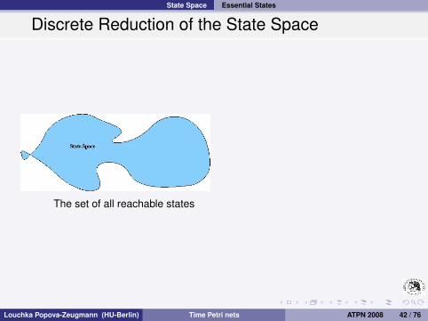
Discrete Reduction of the State Space
The set of all reachable states
The set of all essential states
Louchka Popova-Zeugmann (HU-Berlin) Time Petri nets ATPN 2008 42 / 76

State Space Essential States
Discrete Reduction of the State Space
The set of all reachable states The set of all essential states
Louchka Popova-Zeugmann (HU-Berlin) Time Petri nets ATPN 2008 42 / 76

State Space Reachable Graph
(Reduced) Reachability Graph
The reachability graph is a weighted directed graph, including the timeexplicit.
Louchka Popova-Zeugmann (HU-Berlin) Time Petri nets ATPN 2008 43 / 76

State Space Reachable Graph
(Reduced) Reachability Graph
The reachability graph is a weighted directed graph, including the timeexplicit.
Louchka Popova-Zeugmann (HU-Berlin) Time Petri nets ATPN 2008 43 / 76

State Space Reachable Graph
(Reduced) Reachability Graph
The reachability graph is a weighted directed graph, including the timeexplicit.
Louchka Popova-Zeugmann (HU-Berlin) Time Petri nets ATPN 2008 43 / 76

State Space Reachable Graph
(Reduced) Reachability Graph
The reachability graph is a weighted directed graph, including the timeexplicit.
Louchka Popova-Zeugmann (HU-Berlin) Time Petri nets ATPN 2008 43 / 76

State Space Reachable Graph
(Reduced) Reachability Graph
The reachability graph is a weighted directed graph, including the timeexplicit.
Louchka Popova-Zeugmann (HU-Berlin) Time Petri nets ATPN 2008 43 / 76

State Space Reachable Graph
(Reduced) Reachability Graph
The reachability graph is a weighted directed graph, including the timeexplicit.
Louchka Popova-Zeugmann (HU-Berlin) Time Petri nets ATPN 2008 43 / 76

State Space Reachable Graph
(Reduced) Reachability Graph
The reachability graph is a weighted directed graph, including the timeexplicit.
Louchka Popova-Zeugmann (HU-Berlin) Time Petri nets ATPN 2008 43 / 76

State Space Reachable Graph
(Reduced) Reachability Graph
The reachability graph is a weighted directed graph, including the timeexplicit.
Louchka Popova-Zeugmann (HU-Berlin) Time Petri nets ATPN 2008 43 / 76

State Space Reachable Graph
Example: A finite TPN and its reachability graph
Louchka Popova-Zeugmann (HU-Berlin) Time Petri nets ATPN 2008 44 / 76

State Space Reachable Graph
Example: A finite TPN and its reachability graph
Louchka Popova-Zeugmann (HU-Berlin) Time Petri nets ATPN 2008 44 / 76
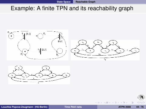
State Space Reachable Graph
Example: A finite TPN and its reachability graph
Louchka Popova-Zeugmann (HU-Berlin) Time Petri nets ATPN 2008 44 / 76

State Space Reachable Graph
Example: A finite TPN and its reachability graph
Louchka Popova-Zeugmann (HU-Berlin) Time Petri nets ATPN 2008 44 / 76

State Space Reachable Graph
Example: A finite TPN and its reachability graph
Louchka Popova-Zeugmann (HU-Berlin) Time Petri nets ATPN 2008 44 / 76

State Space Reachable Graph
Example: A non-finite TPN and its reachabilitygraph
Louchka Popova-Zeugmann (HU-Berlin) Time Petri nets ATPN 2008 45 / 76
Qualitative Analysis Boundedness
Boundedness: TPN vs. Skeleton
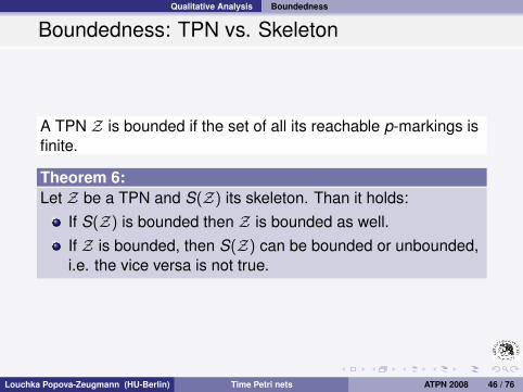
A TPN Z is bounded if the set of all its reachable p-markings isfinite.
Theorem 6:Let Z be a TPN and S(Z) its skeleton. Than it holds:
If S(Z) is bounded then Z is bounded as well.If Z is bounded, then S(Z) can be bounded or unbounded,i.e. the vice versa is not true.
Louchka Popova-Zeugmann (HU-Berlin) Time Petri nets ATPN 2008 46 / 76
Qualitative Analysis Reachability
Reachability in finite TPN
Theorem:Let the skeleton S(Z) of the TPN Z be bounded. Than it holds:
The reachability of each p-marking in Z is decidable.The reachability of each rational state z = (m,h) (i.e. h(t)is a rational number for each enabled transition t by m)is decidable.
Louchka Popova-Zeugmann (HU-Berlin) Time Petri nets ATPN 2008 47 / 76

Qualitative Analysis Reachability
Reachability: TPN vs. Skeleton
Theorem:
Let Z be a TPN, S(Z) its skeleton and eft(t) = 0 for alltransitions t in Z. Than a p-marking m is reachable in Z iff m isreachable in S(Z).
Theorem:
Let Z be a TPN, S(Z) its skeleton and lft(t) =∞ for alltransitions t in Z. Than a p-marking m is reachable in Z iff m isreachable in S(Z).
Let Z be a TPN and z a state in Z. If one of the states bzc ordze are not reachable in Z then z is not reachable in Z as well.
Louchka Popova-Zeugmann (HU-Berlin) Time Petri nets ATPN 2008 48 / 76

Qualitative Analysis Liveness
Liveness: Definitions
Let Z be a TPN, t be a transition in Z and z, z ′ two states in Z.
t is called live in Z, if∀z ∃z ′ ( z0
∗−→ z ∗−→ z ′ t−→ )
t is called dead in Z, if∀z ( z0
∗−→ z t−→′ )
Z is called live or dead, resp., if all transitions in Z are live ordead , resp.
Remark:
There is not a correlation between the liveness behaviors of aTPN and its skeleton.
Louchka Popova-Zeugmann (HU-Berlin) Time Petri nets ATPN 2008 49 / 76

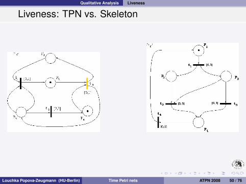
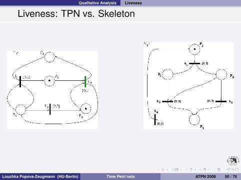
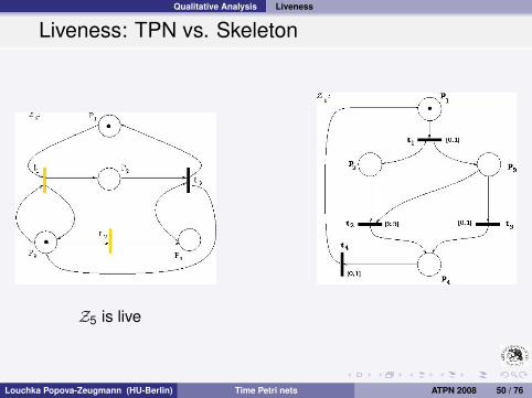
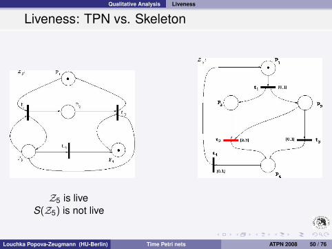
Qualitative Analysis Liveness
Liveness: TPN vs. Skeleton
Z5 is live Z6 is not liveS(Z5) is not live S(Z6) is live
Louchka Popova-Zeugmann (HU-Berlin) Time Petri nets ATPN 2008 50 / 76

Qualitative Analysis Liveness
Liveness: TPN vs. Skeleton
Z5 is live Z6 is not liveS(Z5) is not live S(Z6) is live
Louchka Popova-Zeugmann (HU-Berlin) Time Petri nets ATPN 2008 50 / 76

Qualitative Analysis Liveness
Liveness: TPN vs. Skeleton
Z5 is live Z6 is not liveS(Z5) is not live S(Z6) is live
Louchka Popova-Zeugmann (HU-Berlin) Time Petri nets ATPN 2008 50 / 76

Qualitative Analysis Liveness
Liveness: TPN vs. Skeleton
Z5 is live Z6 is not liveS(Z5) is not live S(Z6) is live
Louchka Popova-Zeugmann (HU-Berlin) Time Petri nets ATPN 2008 50 / 76

Qualitative Analysis Liveness
Liveness: TPN vs. Skeleton
Z5 is live Z6 is not liveS(Z5) is not live S(Z6) is live
Louchka Popova-Zeugmann (HU-Berlin) Time Petri nets ATPN 2008 50 / 76

Qualitative Analysis Liveness
Liveness: TPN vs. Skeleton
Z5 is live Z6 is not liveS(Z5) is not live S(Z6) is live
Louchka Popova-Zeugmann (HU-Berlin) Time Petri nets ATPN 2008 50 / 76

Qualitative Analysis Liveness
Liveness: TPN vs. Skeleton
Z5 is live Z6 is not liveS(Z5) is not live S(Z6) is live
Louchka Popova-Zeugmann (HU-Berlin) Time Petri nets ATPN 2008 50 / 76
Qualitative Analysis Liveness
Liveness: TPN vs. Skeleton
Z5 is live Z6 is not liveS(Z5) is not live S(Z6) is live
Louchka Popova-Zeugmann (HU-Berlin) Time Petri nets ATPN 2008 50 / 76
Qualitative Analysis Liveness
Liveness: TPN vs. Skeleton
Z5 is live Z6 is not liveS(Z5) is not live S(Z6) is live
Louchka Popova-Zeugmann (HU-Berlin) Time Petri nets ATPN 2008 50 / 76

Qualitative Analysis Liveness
Liveness: TPN vs. Skeleton
Z5 is live Z6 is not liveS(Z5) is not live S(Z6) is live
Louchka Popova-Zeugmann (HU-Berlin) Time Petri nets ATPN 2008 50 / 76

Qualitative Analysis Liveness
Liveness: TPN vs. Skeleton
Z5 is live
Z6 is not liveS(Z5) is not live S(Z6) is live
Louchka Popova-Zeugmann (HU-Berlin) Time Petri nets ATPN 2008 50 / 76

Qualitative Analysis Liveness
Liveness: TPN vs. Skeleton
Z5 is live
Z6 is not liveS(Z5) is not live S(Z6) is live
Louchka Popova-Zeugmann (HU-Berlin) Time Petri nets ATPN 2008 50 / 76
Qualitative Analysis Liveness
Liveness: TPN vs. Skeleton
Z5 is live
Z6 is not liveS(Z5) is not live S(Z6) is live
Louchka Popova-Zeugmann (HU-Berlin) Time Petri nets ATPN 2008 50 / 76

Qualitative Analysis Liveness
Liveness: TPN vs. Skeleton
Z5 is live
Z6 is not liveS(Z5) is not live S(Z6) is live
Louchka Popova-Zeugmann (HU-Berlin) Time Petri nets ATPN 2008 50 / 76

Qualitative Analysis Liveness
Liveness: TPN vs. Skeleton
Z5 is live
Z6 is not liveS(Z5) is not live S(Z6) is live
Louchka Popova-Zeugmann (HU-Berlin) Time Petri nets ATPN 2008 50 / 76

Qualitative Analysis Liveness
Liveness: TPN vs. Skeleton
Z5 is live
Z6 is not live
S(Z5) is not live
S(Z6) is live
Louchka Popova-Zeugmann (HU-Berlin) Time Petri nets ATPN 2008 50 / 76
Qualitative Analysis Liveness
Liveness: TPN vs. Skeleton
Z5 is live
Z6 is not live
S(Z5) is not live
S(Z6) is live
Louchka Popova-Zeugmann (HU-Berlin) Time Petri nets ATPN 2008 50 / 76

Qualitative Analysis Liveness
Liveness: TPN vs. Skeleton
Z5 is live Z6 is not liveS(Z5) is not live
S(Z6) is live
Louchka Popova-Zeugmann (HU-Berlin) Time Petri nets ATPN 2008 50 / 76

Qualitative Analysis Liveness
Liveness: TPN vs. Skeleton
Z5 is live Z6 is not liveS(Z5) is not live S(Z6) is live
Louchka Popova-Zeugmann (HU-Berlin) Time Petri nets ATPN 2008 50 / 76

Qualitative Analysis Liveness
Liveness: TPN vs. Skeleton
Theorem:
Let Z be a TPN, S(Z) its skeleton and eft(t) = 0 for alltransitions t in Z. Than Z is live iff S(Z) is live.
Theorem:
Let Z be a TPN, S(Z) its skeleton and lft(t) =∞ for alltransitions t in Z. Than Z is live iff S(Z) is live.
Louchka Popova-Zeugmann (HU-Berlin) Time Petri nets ATPN 2008 51 / 76

Qualitative Analysis Liveness
Liveness: TPN vs. Skeleton
Theorem:
Let Z be a TPN , S(Z) its skeleton such thatS(Z) is a Free-Choice-Net,S(Z) is homogeneous,
and it holds:Min(p) ≤Max(p) for each place p in Z andlft(t) > 0 for each transition t in Z.
Than Z is live iff S(Z) is live.
Louchka Popova-Zeugmann (HU-Berlin) Time Petri nets ATPN 2008 52 / 76

Quantitative Analysis Arbitrary (unbounded or bounded) TPN
Some Decidable Problems without using RG
Problem 1:
Input: A transition sequence σ in an arbitrary TPN Z.
Output: 1 Is σ a firing sequence in Z?2 A feasible run σ(τ) of σ, if the answer to (1) is yes.
Louchka Popova-Zeugmann (HU-Berlin) Time Petri nets ATPN 2008 53 / 76
Quantitative Analysis Arbitrary (unbounded or bounded) TPN
Some Decidable Problems without using RG
Problem 2:
Input: A firing sequence σ in an arbitrary TPN Z.
Output: 1 A minimal run of σ.2 A maximal run of σ, if it exists.
Louchka Popova-Zeugmann (HU-Berlin) Time Petri nets ATPN 2008 54 / 76

Quantitative Analysis Arbitrary (unbounded or bounded) TPN
Some Decidable Problems without using RG
Problem 3:
Input: A TPN Z with an only partially defined interval function I.A transition sequence σ and a number λ ∈ R+
0 .
Output: 1 Is it possible to complete I to a total function such that σis a firing sequence in Z and l
(σ(τ)
)≤ λ?
2 A completed, totally defined function I, if the answer to(1) is yes.
3 Is it possible to complete I to a total function such that σis a firing sequence in Z and l
(σ(τ)
)≥ λ?
4 A completed, total defined function I, if the answer to (3)is yes.
Louchka Popova-Zeugmann (HU-Berlin) Time Petri nets ATPN 2008 55 / 76

Quantitative Analysis Arbitrary (unbounded or bounded) TPN
Some Decidable Problems without using RG
Problem 4:
Input: A TPN Z with an only partially defined interval function I.A transition sequence σ1 = σt1, where σ is a transitionsequence and t1 is a transition in Z.A transition sequence σ2 = σt2, where t2 is a transition inZ such that t1 6= t2.
Output: 1 Is it possible to complete I to a total function such that σ1is a firing sequence in Z and σ2 is not a firing sequenceZ?
2 A completed, totally defined function I, if the answer to(1) is yes.
Louchka Popova-Zeugmann (HU-Berlin) Time Petri nets ATPN 2008 56 / 76

Quantitative Analysis Bounded TPN
Some Decidable Problems with using RG
Problem 5:
Input: Two integer states z1 and z2, reachable in a TPN Z.
Output: 1 Is z2 ∈ RSZ(z1)?2 The minimal time distance from z1 to z2 as well as the
corresponding minimal run, if the answer to (1) is yes.
Louchka Popova-Zeugmann (HU-Berlin) Time Petri nets ATPN 2008 57 / 76

Quantitative Analysis Bounded TPN
Some Decidable Problems with using RG
Problem 6:
Input: Two integer states z1 and z2, reachable in an arbitraryTPN Z.
Output: 1 Is z2 ∈ RSZ(z1)?2 The maximal time distance from z1 to z2 as well as the
corresponding maximal run, if the answer to (1) is yes.
Louchka Popova-Zeugmann (HU-Berlin) Time Petri nets ATPN 2008 58 / 76

Quantitative Analysis Bounded TPN
Some Decidable Problems with using RG
Problem 7:
Input: Two p-markings m1 and m2, reachable in an arbitraryTPN Z.
Output: 1 Is m2 ∈ RZ(m1)?2 The minimal time distance from m1 to m2 as well as the
corresponding minimal run, if the answer to (1) is yes.
Louchka Popova-Zeugmann (HU-Berlin) Time Petri nets ATPN 2008 59 / 76

Quantitative Analysis Bounded TPN
Some Decidable Problems with using RG
Problem 8:
Input: Two p-markings m1 and m2, reachable in an arbitraryTPN Z.
Output: 1 Is m2 ∈ RZ(m1)?2 The maximal time distance from m1 to m2 as well as the
corresponding maximal run, if the answer to (1) is yes.
Louchka Popova-Zeugmann (HU-Berlin) Time Petri nets ATPN 2008 60 / 76

Open Problems
Equivalence of parametric statesImplementation of the quantitative analysis for unbounded TPN
Louchka Popova-Zeugmann (HU-Berlin) Time Petri nets ATPN 2008 61 / 76

Open Problems
Coffee!
Louchka Popova-Zeugmann (HU-Berlin) Time Petri nets ATPN 2008 62 / 76

Open Problems
Coffee!
Louchka Popova-Zeugmann (HU-Berlin) Time Petri nets ATPN 2008 62 / 76
Open Problems
Coffee!
Louchka Popova-Zeugmann (HU-Berlin) Time Petri nets ATPN 2008 62 / 76
Appendix
Petri Net
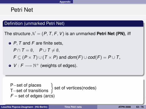
Definition (unmarked Petri Net)
The structure N = (P,T ,F ,V ) is an unmarked Petri Net (PN), iff
P,T and F are finite sets,
P ∩ T = ∅, P ∪ T 6= ∅,F ⊆ (P × T ) ∪ (T × P) and dom(F ) ∪ cod(F ) = P ∪ T ,
V : F −→ N+ (weights of edges).
P−set of placesT−set of transitions
}set of vertices(nodes)
F – set of edges (arcs)
Louchka Popova-Zeugmann (HU-Berlin) Time Petri nets ATPN 2008 63 / 76

Appendix
Petri Net
Definition (marked Petri net)
The structure N0 = (N ,m0) is a marked Petri Net (PN), iff
N is an unmarked PN,
m0 : P −→ N (initial marking).
Louchka Popova-Zeugmann (HU-Berlin) Time Petri nets ATPN 2008 64 / 76

Appendix
Petri Net
Definition (t−, t+)
Let t be a transition in a PN N . t induces the markings t− and t+,
defined as follows:
t−(p) =
{V (p, t) ,iff (p, t) ∈ F
0 ,iff (p, t) 6∈ F
t+(p) =
{V (t ,p) ,iff (t ,p) ∈ F
0 ,iff (t ,p) 6∈ F
Louchka Popova-Zeugmann (HU-Berlin) Time Petri nets ATPN 2008 65 / 76

Appendix
Petri Net
Definition (firing a transition)
A transition t in a PN N is enabled (may fire) at a marking m iff
t− ≤ m (e.g. t−(p) ≤ m(p) for every place p ∈ P).
When an enabled transition t at a marking m fires, this yields a new
marking m′ given by
m′(p) := m(p)− t−(p) + t+(p)
(denoted by m t−→ m′).
Louchka Popova-Zeugmann (HU-Berlin) Time Petri nets ATPN 2008 66 / 76

Appendix
Time Petri Net
Definition (Time Petri net)
The structure Z = (No, I) is called a Time Petri net (TPN) iff:
S(Z) := No is a PN (skeleton of Z)
I : T −→ Q+0 × (Q+
0 ∪ {∞}) and
I1(t) ≤ I2(t) for each t ∈ T , where I(t) = (I1(t), I2(t)).
I − Interval-functionI1(t) =: eft(t)I2(t) =: lft(t)w.o.l.g.: I : T −→ N× (N ∪ {∞})
Louchka Popova-Zeugmann (HU-Berlin) Time Petri nets ATPN 2008 67 / 76

Appendix
state
Definition (state)
Let Z = (P,T ,F ,V ,mo, I) be a TPN and h : T −→ R+0 ∪ {#}.
z = (m,h) is called a state in Z iff:
m is a p-marking in Z .
h is a t-marking in Z.
h(t) is the time shown by the clock of t since the last enabling of t
Louchka Popova-Zeugmann (HU-Berlin) Time Petri nets ATPN 2008 68 / 76

Appendix
Definition (state changing: by time elapsing)
Let Z = (P,T ,F ,V ,mo, I) be a TPN, t̂ be a transition in T and
z = (m,h), z ′ = (m′,h′) be two states. Then the state z = (m,h) is
changed into the state z ′ = (m′,h′) by the time elapsing τ ∈ R+0 ,
denoted by z τ−→ z ′, iff
1 m′ = m and
2 ∀t ( t ∈ T ∧ h(t) 6= # −→ h(t) + τ ≤ lft(t) ) i.e. the time elapsing τ
is possible, and
3 ∀t ( t ∈ T −→ h′(t) :=
{h(t) + τ iff t− ≤ m′
# iff t− 6≤ m′).
Louchka Popova-Zeugmann (HU-Berlin) Time Petri nets ATPN 2008 69 / 76
Appendix
Definition (state changing: by firing a transition)
Let Z = (P,T ,F ,V ,mo, I) be a TPN, t̂ be a transition in T and
z = (m,h), z ′ = (m′,h′) be two states. Then the state z = (m,h) is
changed into the state z ′ = (m′,h′) by firing the transition t̂ , denoted
by z t̂−→ z ′ , iff
1 t̂− ≤ m, i.e. t̂ is enabled in z
2 eft (̂t) ≤ h(̂t), i.e. t̂ is old enough in z,
3 m′ = m + ∆t̂
4 h′(t) :=
# iff t− 6≤ m′
h(t) iff t− ≤ m ∧ t− ≤ m′∧•t ∩ • t̂ = ∅ ∧ t 6= t̂
0 otherwise
for each t ∈ T .
Louchka Popova-Zeugmann (HU-Berlin) Time Petri nets ATPN 2008 70 / 76

Appendix
Definition (state changing: by firing a transition)
Let Z = (P,T ,F ,V ,mo, I) be a TPN, t̂ be a transition in T and
z = (m,h), z ′ = (m′,h′) be two states. Then the state z = (m,h) is
changed into the state z ′ = (m′,h′) by firing the transition t̂ , denoted
by z t̂−→ z ′ , iff
1 t̂− ≤ m, i.e. t̂ is enabled in z
2 eft (̂t) ≤ h(̂t), i.e. t̂ is old enough in z,
3 m′ = m + ∆t̂
4 h′(t) :=
# iff t− 6≤ m′
h(t) iff t− ≤ m ∧
t− ≤ m′∧
•t ∩ • t̂ = ∅ ∧ t 6= t̂
0 otherwise
for each t ∈ T .
Louchka Popova-Zeugmann (HU-Berlin) Time Petri nets ATPN 2008 70 / 76

Appendix
Modified Rule for Time Elapsing
Definition
Let Z = (P,T ,F ,V ,mo, I) be a TPN, t̂ be a transition in T andz = (m,h), z ′ = (m′,h′) be two states. Then the state z = (m,h) ischanged into the state z ′ = (m′,h′) by the time elapsing τ ∈ R+
0 ,denoted by z τ−→ z ′, iff
1 m′ = m and2 ∀t ( t ∈ T ∧ h(t) 6= # −→ h(t) + τ ≤ lft(t) ) i.e. the time elapsing τ
is possible, and
3 ∀t ( t ∈ T −→ h′(t) :=
# iff t− 6≤ m′
h(t) iff t− ≤ m′ ∧ lft(t) =∞∧h(t) ≥ eft(t)
h(t) + τ else
).
Louchka Popova-Zeugmann (HU-Berlin) Time Petri nets ATPN 2008 71 / 76

Appendix
z00.7
1
−→ t1−→ 0.0
0
−→ t3−→ 0.4
1
−→ t4−→ 1.2
1
−→ t2−→ 0.5
0
−→ t3−→ 1.4
1
−→`mσ, (1.9, 1.4, 1.4, 1.4, 4.2, ])
´
I x0 x1 x2 x3 x4 x5 hσ(t1) hσ(t2) hσ(t5)
β̂ = β0 0.7 0.0 0.4 1.2 0.5 1.4 1.9 1.4 4.2
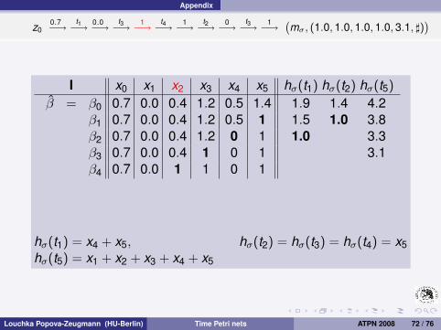
β1 0.7 0.0 0.4 1.2 0.5 1 1.5 1.0 3.8β2 0.7 0.0 0.4 1.2 0 1 1.0 3.3β3 0.7 0.0 0.4 1 0 1 3.1β4 0.7 0.0 1 1 0 1 3.7β5 0.7 0 1 1 0 1 3.7
β∗ = β6 1 0 1 1 0 1 4.0
hσ(t1) = x4 + x5, hσ(t2) = hσ(t3) = hσ(t4) = x5hσ(t5) = x1 + x2 + x3 + x4 + x5
Louchka Popova-Zeugmann (HU-Berlin) Time Petri nets ATPN 2008 72 / 76

Appendix
z00.7
1
−→ t1−→ 0.0
0
−→ t3−→ 0.4
1
−→ t4−→ 1.2
1
−→ t2−→ 0.5
0
−→ t3−→ 1.4
1
−→`mσ, (1.9, 1.4, 1.4, 1.4, 4.2, ])
´
I x0 x1 x2 x3 x4 x5 hσ(t1) hσ(t2) hσ(t5)
β̂ = β0 0.7 0.0 0.4 1.2 0.5 1.4 1.9 1.4 4.2β1 0.7 0.0 0.4 1.2 0.5
1 1.5 1.0 3.8β2 0.7 0.0 0.4 1.2 0 1 1.0 3.3β3 0.7 0.0 0.4 1 0 1 3.1β4 0.7 0.0 1 1 0 1 3.7β5 0.7 0 1 1 0 1 3.7
β∗ = β6 1 0 1 1 0 1 4.0
hσ(t1) = x4 + x5, hσ(t2) = hσ(t3) = hσ(t4) = x5hσ(t5) = x1 + x2 + x3 + x4 + x5
Louchka Popova-Zeugmann (HU-Berlin) Time Petri nets ATPN 2008 72 / 76

Appendix
z00.7
1
−→ t1−→ 0.0
0
−→ t3−→ 0.4
1
−→ t4−→ 1.2
1
−→ t2−→ 0.5
0
−→ t3−→ 1−→`mσ, (1.9, 1.4, 1.4, 1.4, 4.2, ])
´
I x0 x1 x2 x3 x4 x5 hσ(t1) hσ(t2) hσ(t5)
β̂ = β0 0.7 0.0 0.4 1.2 0.5 1.4 1.9 1.4 4.2β1 0.7 0.0 0.4 1.2 0.5 1
1.5 1.0 3.8β2 0.7 0.0 0.4 1.2 0 1 1.0 3.3β3 0.7 0.0 0.4 1 0 1 3.1β4 0.7 0.0 1 1 0 1 3.7β5 0.7 0 1 1 0 1 3.7
β∗ = β6 1 0 1 1 0 1 4.0
hσ(t1) = x4 + x5, hσ(t2) = hσ(t3) = hσ(t4) = x5hσ(t5) = x1 + x2 + x3 + x4 + x5
Louchka Popova-Zeugmann (HU-Berlin) Time Petri nets ATPN 2008 72 / 76

Appendix
z00.7
1
−→ t1−→ 0.0
0
−→ t3−→ 0.4
1
−→ t4−→ 1.2
1
−→ t2−→ 0.5
0
−→ t3−→ 1−→`mσ, (1.5, 1.0, 1.0, 1.0, 3.8, ])
´
I x0 x1 x2 x3 x4 x5 hσ(t1) hσ(t2) hσ(t5)
β̂ = β0 0.7 0.0 0.4 1.2 0.5 1.4 1.9 1.4 4.2β1 0.7 0.0 0.4 1.2 0.5 1 1.5 1.0 3.8
β2 0.7 0.0 0.4 1.2 0 1 1.0 3.3β3 0.7 0.0 0.4 1 0 1 3.1β4 0.7 0.0 1 1 0 1 3.7β5 0.7 0 1 1 0 1 3.7
β∗ = β6 1 0 1 1 0 1 4.0
hσ(t1) = x4 + x5, hσ(t2) = hσ(t3) = hσ(t4) = x5hσ(t5) = x1 + x2 + x3 + x4 + x5
Louchka Popova-Zeugmann (HU-Berlin) Time Petri nets ATPN 2008 72 / 76

Appendix
z00.7
1
−→ t1−→ 0.0
0
−→ t3−→ 0.4
1
−→ t4−→ 1.2
1
−→ t2−→ 0.5
0
−→ t3−→ 1−→`mσ, (1.5, 1.0, 1.0, 1.0, 3.8, ])
´
I x0 x1 x2 x3 x4 x5 hσ(t1) hσ(t2) hσ(t5)
β̂ = β0 0.7 0.0 0.4 1.2 0.5 1.4 1.9 1.4 4.2β1 0.7 0.0 0.4 1.2 0.5 1 1.5 1.0 3.8β2 0.7 0.0 0.4 1.2
0
1
1.0 3.3β3 0.7 0.0 0.4 1 0 1 3.1β4 0.7 0.0 1 1 0 1 3.7β5 0.7 0 1 1 0 1 3.7
β∗ = β6 1 0 1 1 0 1 4.0
hσ(t1) = x4 + x5, hσ(t2) = hσ(t3) = hσ(t4) = x5hσ(t5) = x1 + x2 + x3 + x4 + x5
Louchka Popova-Zeugmann (HU-Berlin) Time Petri nets ATPN 2008 72 / 76

Appendix
z00.7
1
−→ t1−→ 0.0
0
−→ t3−→ 0.4
1
−→ t4−→ 1.2
1
−→ t2−→ 0−→ t3−→ 1−→`mσ, (1.5, 1.0, 1.0, 1.0, 3.8, ])
´
I x0 x1 x2 x3 x4 x5 hσ(t1) hσ(t2) hσ(t5)
β̂ = β0 0.7 0.0 0.4 1.2 0.5 1.4 1.9 1.4 4.2β1 0.7 0.0 0.4 1.2 0.5 1 1.5 1.0 3.8β2 0.7 0.0 0.4 1.2 0 1
1.0 3.3β3 0.7 0.0 0.4 1 0 1 3.1β4 0.7 0.0 1 1 0 1 3.7β5 0.7 0 1 1 0 1 3.7
β∗ = β6 1 0 1 1 0 1 4.0
hσ(t1) = x4 + x5, hσ(t2) = hσ(t3) = hσ(t4) = x5hσ(t5) = x1 + x2 + x3 + x4 + x5
Louchka Popova-Zeugmann (HU-Berlin) Time Petri nets ATPN 2008 72 / 76

Appendix
z00.7
1
−→ t1−→ 0.0
0
−→ t3−→ 0.4
1
−→ t4−→ 1.2
1
−→ t2−→ 0−→ t3−→ 1−→`mσ, (1.0, 1.0, 1.0, 1.0, 3.3, ])
´
I x0 x1 x2 x3 x4 x5 hσ(t1) hσ(t2) hσ(t5)
β̂ = β0 0.7 0.0 0.4 1.2 0.5 1.4 1.9 1.4 4.2β1 0.7 0.0 0.4 1.2 0.5 1 1.5 1.0 3.8β2 0.7 0.0 0.4 1.2 0 1 1.0 3.3
β3 0.7 0.0 0.4 1 0 1 3.1β4 0.7 0.0 1 1 0 1 3.7β5 0.7 0 1 1 0 1 3.7
β∗ = β6 1 0 1 1 0 1 4.0
hσ(t1) = x4 + x5, hσ(t2) = hσ(t3) = hσ(t4) = x5hσ(t5) = x1 + x2 + x3 + x4 + x5
Louchka Popova-Zeugmann (HU-Berlin) Time Petri nets ATPN 2008 72 / 76

Appendix
z00.7
1
−→ t1−→ 0.0
0
−→ t3−→ 0.4
1
−→ t4−→ 1.2
1
−→ t2−→ 0−→ t3−→ 1−→`mσ, (1.0, 1.0, 1.0, 1.0, 3.3, ])
´
I x0 x1 x2 x3 x4 x5 hσ(t1) hσ(t2) hσ(t5)
β̂ = β0 0.7 0.0 0.4 1.2 0.5 1.4 1.9 1.4 4.2β1 0.7 0.0 0.4 1.2 0.5 1 1.5 1.0 3.8β2 0.7 0.0 0.4 1.2 0 1 1.0 3.3β3 0.7 0.0 0.4
1
0 1
3.1β4 0.7 0.0 1 1 0 1 3.7β5 0.7 0 1 1 0 1 3.7
β∗ = β6 1 0 1 1 0 1 4.0
hσ(t1) = x4 + x5, hσ(t2) = hσ(t3) = hσ(t4) = x5hσ(t5) = x1 + x2 + x3 + x4 + x5
Louchka Popova-Zeugmann (HU-Berlin) Time Petri nets ATPN 2008 72 / 76

Appendix
z00.7
1
−→ t1−→ 0.0
0
−→ t3−→ 0.4
1
−→ t4−→ 1−→ t2−→ 0−→ t3−→ 1−→`mσ, (1.0, 1.0, 1.0, 1.0, 3.3, ])
´
I x0 x1 x2 x3 x4 x5 hσ(t1) hσ(t2) hσ(t5)
β̂ = β0 0.7 0.0 0.4 1.2 0.5 1.4 1.9 1.4 4.2β1 0.7 0.0 0.4 1.2 0.5 1 1.5 1.0 3.8β2 0.7 0.0 0.4 1.2 0 1 1.0 3.3β3 0.7 0.0 0.4 1 0 1
3.1β4 0.7 0.0 1 1 0 1 3.7β5 0.7 0 1 1 0 1 3.7
β∗ = β6 1 0 1 1 0 1 4.0
hσ(t1) = x4 + x5, hσ(t2) = hσ(t3) = hσ(t4) = x5hσ(t5) = x1 + x2 + x3 + x4 + x5
Louchka Popova-Zeugmann (HU-Berlin) Time Petri nets ATPN 2008 72 / 76

Appendix
z00.7
1
−→ t1−→ 0.0
0
−→ t3−→ 0.4
1
−→ t4−→ 1−→ t2−→ 0−→ t3−→ 1−→`mσ, (1.0, 1.0, 1.0, 1.0, 3.1, ])
´
I x0 x1 x2 x3 x4 x5 hσ(t1) hσ(t2) hσ(t5)
β̂ = β0 0.7 0.0 0.4 1.2 0.5 1.4 1.9 1.4 4.2β1 0.7 0.0 0.4 1.2 0.5 1 1.5 1.0 3.8β2 0.7 0.0 0.4 1.2 0 1 1.0 3.3β3 0.7 0.0 0.4 1 0 1 3.1
β4 0.7 0.0 1 1 0 1 3.7β5 0.7 0 1 1 0 1 3.7
β∗ = β6 1 0 1 1 0 1 4.0
hσ(t1) = x4 + x5, hσ(t2) = hσ(t3) = hσ(t4) = x5hσ(t5) = x1 + x2 + x3 + x4 + x5
Louchka Popova-Zeugmann (HU-Berlin) Time Petri nets ATPN 2008 72 / 76

Appendix
z00.7
1
−→ t1−→ 0.0
0
−→ t3−→ 0.4
1
−→ t4−→ 1−→ t2−→ 0−→ t3−→ 1−→`mσ, (1.0, 1.0, 1.0, 1.0, 3.1, ])
´
I x0 x1 x2 x3 x4 x5 hσ(t1) hσ(t2) hσ(t5)
β̂ = β0 0.7 0.0 0.4 1.2 0.5 1.4 1.9 1.4 4.2β1 0.7 0.0 0.4 1.2 0.5 1 1.5 1.0 3.8β2 0.7 0.0 0.4 1.2 0 1 1.0 3.3β3 0.7 0.0 0.4 1 0 1 3.1β4 0.7 0.0
1
1 0 1
3.7β5 0.7 0 1 1 0 1 3.7
β∗ = β6 1 0 1 1 0 1 4.0
hσ(t1) = x4 + x5, hσ(t2) = hσ(t3) = hσ(t4) = x5hσ(t5) = x1 + x2 + x3 + x4 + x5
Louchka Popova-Zeugmann (HU-Berlin) Time Petri nets ATPN 2008 72 / 76
Appendix
z00.7
1
−→ t1−→ 0.0
0
−→ t3−→ 1−→ t4−→ 1−→ t2−→ 0−→ t3−→ 1−→`mσ, (1.0, 1.0, 1.0, 1.0, 3.1, ])
´
I x0 x1 x2 x3 x4 x5 hσ(t1) hσ(t2) hσ(t5)
β̂ = β0 0.7 0.0 0.4 1.2 0.5 1.4 1.9 1.4 4.2β1 0.7 0.0 0.4 1.2 0.5 1 1.5 1.0 3.8β2 0.7 0.0 0.4 1.2 0 1 1.0 3.3β3 0.7 0.0 0.4 1 0 1 3.1β4 0.7 0.0 1 1 0 1
3.7β5 0.7 0 1 1 0 1 3.7
β∗ = β6 1 0 1 1 0 1 4.0
hσ(t1) = x4 + x5, hσ(t2) = hσ(t3) = hσ(t4) = x5hσ(t5) = x1 + x2 + x3 + x4 + x5
Louchka Popova-Zeugmann (HU-Berlin) Time Petri nets ATPN 2008 72 / 76

Appendix
z00.7
1
−→ t1−→ 0.0
0
−→ t3−→ 1−→ t4−→ 1−→ t2−→ 0−→ t3−→ 1−→`mσ, (1.0, 1.0, 1.0, 1.0, 3.7, ])
´
I x0 x1 x2 x3 x4 x5 hσ(t1) hσ(t2) hσ(t5)
β̂ = β0 0.7 0.0 0.4 1.2 0.5 1.4 1.9 1.4 4.2β1 0.7 0.0 0.4 1.2 0.5 1 1.5 1.0 3.8β2 0.7 0.0 0.4 1.2 0 1 1.0 3.3β3 0.7 0.0 0.4 1 0 1 3.1β4 0.7 0.0 1 1 0 1 3.7
β5 0.7 0 1 1 0 1 3.7β∗ = β6 1 0 1 1 0 1 4.0
hσ(t1) = x4 + x5, hσ(t2) = hσ(t3) = hσ(t4) = x5hσ(t5) = x1 + x2 + x3 + x4 + x5
Louchka Popova-Zeugmann (HU-Berlin) Time Petri nets ATPN 2008 72 / 76

Appendix
z00.7
1
−→ t1−→ 0.0
0
−→ t3−→ 1−→ t4−→ 1−→ t2−→ 0−→ t3−→ 1−→`mσ, (1.0, 1.0, 1.0, 1.0, 3.7, ])
´
I x0 x1 x2 x3 x4 x5 hσ(t1) hσ(t2) hσ(t5)
β̂ = β0 0.7 0.0 0.4 1.2 0.5 1.4 1.9 1.4 4.2β1 0.7 0.0 0.4 1.2 0.5 1 1.5 1.0 3.8β2 0.7 0.0 0.4 1.2 0 1 1.0 3.3β3 0.7 0.0 0.4 1 0 1 3.1β4 0.7 0.0 1 1 0 1 3.7β5 0.7
0
1 1 0 1
3.7β∗ = β6 1 0 1 1 0 1 4.0
hσ(t1) = x4 + x5, hσ(t2) = hσ(t3) = hσ(t4) = x5hσ(t5) = x1 + x2 + x3 + x4 + x5
Louchka Popova-Zeugmann (HU-Berlin) Time Petri nets ATPN 2008 72 / 76
Appendix
z00.7
1
−→ t1−→ 0−→ t3−→ 1−→ t4−→ 1−→ t2−→ 0−→ t3−→ 1−→`mσ, (1.0, 1.0, 1.0, 1.0, 3.7, ])
´
I x0 x1 x2 x3 x4 x5 hσ(t1) hσ(t2) hσ(t5)
β̂ = β0 0.7 0.0 0.4 1.2 0.5 1.4 1.9 1.4 4.2β1 0.7 0.0 0.4 1.2 0.5 1 1.5 1.0 3.8β2 0.7 0.0 0.4 1.2 0 1 1.0 3.3β3 0.7 0.0 0.4 1 0 1 3.1β4 0.7 0.0 1 1 0 1 3.7β5 0.7 0 1 1 0 1
3.7β∗ = β6 1 0 1 1 0 1 4.0
hσ(t1) = x4 + x5, hσ(t2) = hσ(t3) = hσ(t4) = x5hσ(t5) = x1 + x2 + x3 + x4 + x5
Louchka Popova-Zeugmann (HU-Berlin) Time Petri nets ATPN 2008 72 / 76

Appendix
z00.7
1
−→ t1−→ 0−→ t3−→ 1−→ t4−→ 1−→ t2−→ 0−→ t3−→ 1−→`mσ, (1.0, 1.0, 1.0, 1.0, 3.7, ])
´
I x0 x1 x2 x3 x4 x5 hσ(t1) hσ(t2) hσ(t5)
β̂ = β0 0.7 0.0 0.4 1.2 0.5 1.4 1.9 1.4 4.2β1 0.7 0.0 0.4 1.2 0.5 1 1.5 1.0 3.8β2 0.7 0.0 0.4 1.2 0 1 1.0 3.3β3 0.7 0.0 0.4 1 0 1 3.1β4 0.7 0.0 1 1 0 1 3.7β5 0.7 0 1 1 0 1 3.7
β∗ = β6 1 0 1 1 0 1 4.0
hσ(t1) = x4 + x5, hσ(t2) = hσ(t3) = hσ(t4) = x5hσ(t5) = x1 + x2 + x3 + x4 + x5
Louchka Popova-Zeugmann (HU-Berlin) Time Petri nets ATPN 2008 72 / 76
Appendix
z00.7
1
−→ t1−→ 0−→ t3−→ 1−→ t4−→ 1−→ t2−→ 0−→ t3−→ 1−→`mσ, (1.0, 1.0, 1.0, 1.0, 3.7, ])
´
I x0 x1 x2 x3 x4 x5 hσ(t1) hσ(t2) hσ(t5)
β̂ = β0 0.7 0.0 0.4 1.2 0.5 1.4 1.9 1.4 4.2β1 0.7 0.0 0.4 1.2 0.5 1 1.5 1.0 3.8β2 0.7 0.0 0.4 1.2 0 1 1.0 3.3β3 0.7 0.0 0.4 1 0 1 3.1β4 0.7 0.0 1 1 0 1 3.7β5 0.7 0 1 1 0 1 3.7
β∗ = β6
1
0 1 1 0 1
4.0
hσ(t1) = x4 + x5, hσ(t2) = hσ(t3) = hσ(t4) = x5hσ(t5) = x1 + x2 + x3 + x4 + x5
Louchka Popova-Zeugmann (HU-Berlin) Time Petri nets ATPN 2008 72 / 76

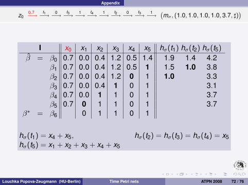
Appendix
z01−→ t1−→ 0−→ t3−→ 1−→ t4−→ 1−→ t2−→ 0−→ t3−→ 1−→
`mσ, (1.0, 1.0, 1.0, 1.0, 3.7, ])
´
I x0 x1 x2 x3 x4 x5 hσ(t1) hσ(t2) hσ(t5)
β̂ = β0 0.7 0.0 0.4 1.2 0.5 1.4 1.9 1.4 4.2β1 0.7 0.0 0.4 1.2 0.5 1 1.5 1.0 3.8β2 0.7 0.0 0.4 1.2 0 1 1.0 3.3β3 0.7 0.0 0.4 1 0 1 3.1β4 0.7 0.0 1 1 0 1 3.7β5 0.7 0 1 1 0 1 3.7
β∗ = β6 1 0 1 1 0 1
4.0
hσ(t1) = x4 + x5, hσ(t2) = hσ(t3) = hσ(t4) = x5hσ(t5) = x1 + x2 + x3 + x4 + x5
Louchka Popova-Zeugmann (HU-Berlin) Time Petri nets ATPN 2008 72 / 76

Appendix
z01−→ t1−→ 0−→ t3−→ 1−→ t4−→ 1−→ t2−→ 0−→ t3−→ 1−→
`mσ, (1.0, 1.0, 1.0, 1.0, 4.0, ])
´
I x0 x1 x2 x3 x4 x5 hσ(t1) hσ(t2) hσ(t5)
β̂ = β0 0.7 0.0 0.4 1.2 0.5 1.4 1.9 1.4 4.2β1 0.7 0.0 0.4 1.2 0.5 1 1.5 1.0 3.8β2 0.7 0.0 0.4 1.2 0 1 1.0 3.3β3 0.7 0.0 0.4 1 0 1 3.1β4 0.7 0.0 1 1 0 1 3.7β5 0.7 0 1 1 0 1 3.7
β∗ = β6 1 0 1 1 0 1 4.0
hσ(t1) = x4 + x5, hσ(t2) = hσ(t3) = hσ(t4) = x5hσ(t5) = x1 + x2 + x3 + x4 + x5
Louchka Popova-Zeugmann (HU-Berlin) Time Petri nets ATPN 2008 72 / 76

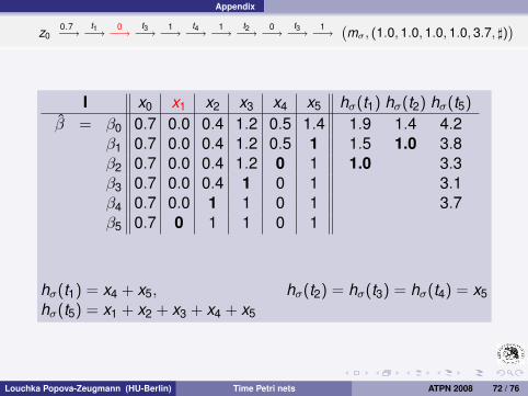
Appendix
z00.7−→ t1−→ 0.0−→ t3−→ 0.4−→ t4−→ 1.2−→ t2−→ 0.5−→ t3−→ 1.4−→
`mσ, (1.9, 1.4, 1.4, 1.4, 4.2, ])
´
II x0 x1 x2 x3 x4 x5 hσ(t1) hσ(t2) hσ(t5)
β̂ = β0 0.7 0.0 0.4 1.2 0.5 1.4 1.9 1.4 4.2β1 0.7 0.0 0.4 1.2 0.5 2 2.5 2.0 4.8β2 0.7 0.0 0.4 1.2 0 2 2.0 4.3β3 0.7 0.0 0.4 2 0 2 5.1β4 0.7 0.0 0 2 0 2 4.7β5 0.7 0 0 2 0 2 4.7β6 1 0 0 2 0 2 5.0
z01−→ t1−→ 0−→ t3−→ 0−→ t4−→ 2−→ t2−→ 0−→ t3−→ 2−→
`mσ, (2, 2, 2, 2, 5, ])
´
Louchka Popova-Zeugmann (HU-Berlin) Time Petri nets ATPN 2008 73 / 76

Appendix
z00.7−→ t1−→ 0.0−→ t3−→ 0.4−→ t4−→ 1.2−→ t2−→ 0.5−→ t3−→ 1.4−→
`mσ, (1.9, 1.4, 1.4, 1.4, 4.2, ])
´
The time length of the run σ(τ) is
β̂(x0) + β̂(x1) + β̂(x2) + β̂(x3) + β̂(x4) + β̂(x5) = 4.2
In tableau I: The time length of the run σ(τ∗1 ) is 4
In tableau II: The time length of the run σ(τ∗2 ) is 5
Louchka Popova-Zeugmann (HU-Berlin) Time Petri nets ATPN 2008 74 / 76
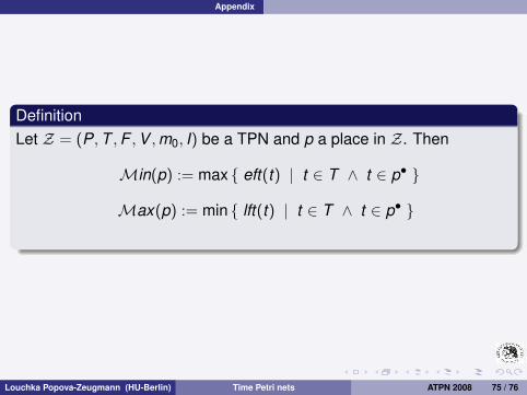
Appendix
DefinitionLet Z = (P,T ,F ,V ,m0, I) be a TPN and p a place in Z. Then
Min(p) := max { eft(t) | t ∈ T ∧ t ∈ p• }
Max(p) := min { lft(t) | t ∈ T ∧ t ∈ p• }
Louchka Popova-Zeugmann (HU-Berlin) Time Petri nets ATPN 2008 75 / 76
Appendix
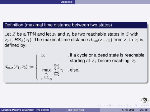
Definition (maximal time distance between two states)
Let Z be a TPN and let z1 and z2 be two reachable states in Z withz2 ∈ RSZ(z1). The maximal time distance dmax(z1, z2) from z1 to z2 isdefined by:
dmax(z1, z2) :=
∞ , if a cycle or a dead state is reachable
starting at z1 before reaching z2
maxσ,
z1σ(τ)−→ z2
l(τ)∑i=0
τi , else.
Louchka Popova-Zeugmann (HU-Berlin) Time Petri nets ATPN 2008 76 / 76