NASA Contractor Report 198274

1CASE Report No. 96-5

,

ICA

FLUID STOCHASTIC PETRI NETS:

THEORY, APPLICATIONS, AND SOLUTION

Graham Horton

Vidyadhar G. KulkarniDavid M. Nicol

Kishor S. Trivedi

NASA Contract No. NAS1-19480

January 1996

Institute for Computer Applications in Science and Engineering

NASA Langley Research Center

Hampton, VA 23681-0001

Operated by Universities Space Research Association

National Aeronautics and

Space Administration

Langley Research Center

Hampton, Virginia 23681-0001

https://ntrs.nasa.gov/search.jsp?R=19960018542 2018-09-01T11:43:25+00:00Z

Fluid Stochastic Petri Nets: Theory, Applications, and Solution 1

Graham Horton 4, Vidyadhar G. Kulkarni s, David M. Nicol _ and Kishor S. Trivedi 3

4Lehrstuhl ffir Rechnerstrukturen (IMMD 3),

Universit_t Erlangen-Nfirnberg, Martensstr. 3,

91058 Erlangen, Germany.

5Department of Operations Research

University of North Carolina, Chapel Hill, NC 27599, U.S.A.

2Department of Computer Science

College of William and Mary, Williamsburg, VA 23187-8795, U.S.A.

3Center for Advanced Computing and Communication

Department of Electrical and Computer Engineering

Duke University, Durham, NC 27708-0291, U.S.A.

Abstract

In this paper we introduce a new class of stochastic Petri nets in which one or more places can hold fluid rather

than discrete tokens. We define a class of fluid stochastic Petri nets in such a way that the discrete and continuous

portions may affect each other. Following this definition we provide equations for their transient and steady-state

behavior. We present several examples showing the utility of the construct in communication network modeling

and reliability analysis, and discuss important special cases. We then discuss numerical methods for computing the

transient behavior of such nets. FinaJly, some numerical examples are presented.

1A preliminary version of this paper appeared in the Proceedings of the 1993 Petri Net Conference, Chicago, Illinois, under

the title FSPNs: Fluid Stochastic Petri Nets. This research was partially supported by the National Aeronautics and Space

Administration under NASA contract NAS1-19480 while the first, third and fourth authors were in residence at the Institute

for Computer Applications in Science and Engineering (ICASE), NASA Langley Research Center, Hampton, VA 23681-0001.

2This research was supported in part by the National Science Foundation under Grant CCR-9201195 and by NASA Grant

NAG-1332.

3This research was supported in part by the National Science Foundation under Grant NSF-EEC-94-18765.

1 Introduction

One of the difficulties encountered while using Petri nets is that the reachability graph tends to be very large

in practical problems. Drawing a parallel with fluid flow approximations in performance analysis of queueing

systems, we may define fluid within a Petri-net to approximate token movement. Alternatively, some physical

systems have not previously admitted a Petri net modeling approach, as they explicitly contain continuous

fluid-like quantities which are controlled with discrete logic. This paper presents a new methodology for

modeling such systems.

Stochastic fluid flow models are increasingly used in the performance analysis of communications [3, 10, 13]

and manufacturing systems. On the other hand, stochastic Petri nets with discrete places provide a useful

framework for specifying and solving performance and reliability models of discrete event dynamic systems

[1, 6, 9, 17, 19]. It is natural to extend the stochastic Petri net framework to Fluid Stochastic Petri Nets

(FSPNs) by introducing places with continuous tokens and arcs with fluid flow so as to handle stochastic

fluid flow systems. This paper extends the model in an earlier paper [18] by allowing the level of fluid

in continuous places to affect the enabling of timed transitions and the rates of fluid flow into and out

of continuous places. Rules for transition enabling and firing are extended to reflect the notion that flow

through a fluid place represents token movement.

An FSPN contains two types of places: discrete places containing a non-negative integer number of

tokens, and continuous places containing fluid. Transition firings are determined by both discrete places

and continuous places, and fluid flow is permitted through the enabled timed transitions in the Petri net.

Associating exponentially distributed or zero firing time with transitions, we can then write the differential

equations for the underlying stochastic process. We also provide additional examples of FSPN usage, and

discuss numerical issues arising in the solution of the underlying dynamic equations.

The main motivation of this paper is to put the research by Mitra and his colleagues [3, 10, 13] in the

context of Petri nets, to make some extensions and to investigate the numerical transient analysis of such

stochastic fluid models.

The paper is organized as follows. In Section 2 we develop the fluid model of stochastic Petri nets and in

Section 3 we discuss their analysis. Examples and special cases are described in Section 4, numerical solution

techniques are described in Section 5, while numerical examples are given in Section 6. The paper concludes

in Section 7.

2 The Stochastic Fluid Model

Following the customary notation [8, 14, 16] for defining Petri nets and their extensions, we define a fluid

stochastic Petri net (FSPN) as a 8-tuple (P, _r, A, rn0, Y, )'Y, 7_, _ ). "P is a set of places partitioned into a

setofdiscreteplacesPd and a set of continuous places "Pc. The number of fluid places is F _> 0, indexed by

k = 1, 2, - •., F. In a graphical representation, we shall depict continuous places by means of two concentric

circles. The set of transitions 7" is partitioned into a set of (exponentially distributed firing) timed transitions

7"E and a set of immediate transitions 7). The set of directed arcs A is partitioned into two subsets Ac and

•Ad. Ac is a subset of ('pc x tiE) t.I (7-E × "pc) while Ad is a subset of ('Pd x 7-) O (7- x "pd). In a graphical

representation, arcs in Ac are drawn as double lines (to suggest a pipe) while those in .Ad are drawn as single

lines.

Let md= (_Pi, i E "pal) be the vector of the number of tokens in discrete places and let _ = (xk, k E "pc)

be the vector of the fluid levels in continuous places. We will say that md is the discrete marking of the

net. Let M denote the number of discrete markings, which will be indexed by the symbols i and j, with

i, j = 1, 2,-. -, M. The complete state (marking) of a fluid Petri net is described by the vector m = (g, rod)

where md is the marking of the discrete part of the state and £ keeps track of the fluid levels in the continuous

places. Let .M be the set of all complete markings (£, rod) and .Md be the set of all discrete markings. The

initial marking is m0 = (£0, redO).

In our formulation an enabled transition in 7"E may drain fluid out of its continuous input places, and

may pump fluid into its continuous output places. The rates of flow may be dependent on the complete

marking (£, rod). In a general formulation of a stochastic Petri net (embodied, for example, by SPNP [7, 8])

the conditions for enabling can be specified either through explicit arcs or through Boolean functions known

as guards. We will allow both of these possibilities. We will continue to use the enabling and firing rules

employed in SPNP with the additional possibility of a guard associated with a timed transition being able

to base the enabling condition not only on the discrete marking of the net but also on the continuous part.

We disallow the enabling of immediate transitions by fluid levels as this would lead to g-dependent vanishing

markings, which cannot be eliminated in a manner analogous to that of GSPNs. Thus the guard function

is defined for any timed transition in TE so that _ : 7" × A4 --* {0, 1}. For a timed transition 7"E TE, _(r, m)

is a Boolean function that will be evaluated in each marking, and if it evaluates to true, the transition

may be enabled; otherwise v is disabled. Upon firing, the transition removes a specified number of tokens

from each discrete input place, and deposits a specified number of tokens in each discrete output place.

The basic extension we have made from [18] here is that fluid levels in continuous places can change the

enabling/disabling of timed transitions in the discrete part of the net. A discrete marking rnd is said to be a

vanishing marking if one or more immediate transitions are enabled by it; otherwise it is a tangible marking.

The firing rate function Y is defined for timed transitions 7-E so that Y : 7"E x .hal --. IR+. Thus if a

timed transition 7"is enabled in (tangible) marking m, it fires with rate .T(v, m). Note once again that in

[18], these rates were not allowed to depend upon the fluid levels but now we do allow the firing rates to be

dependent on fluid levels.

As in [18], the weight function W is defined for immediate transitions 7) so that 14; : 7-I × .Md ---, IR+.

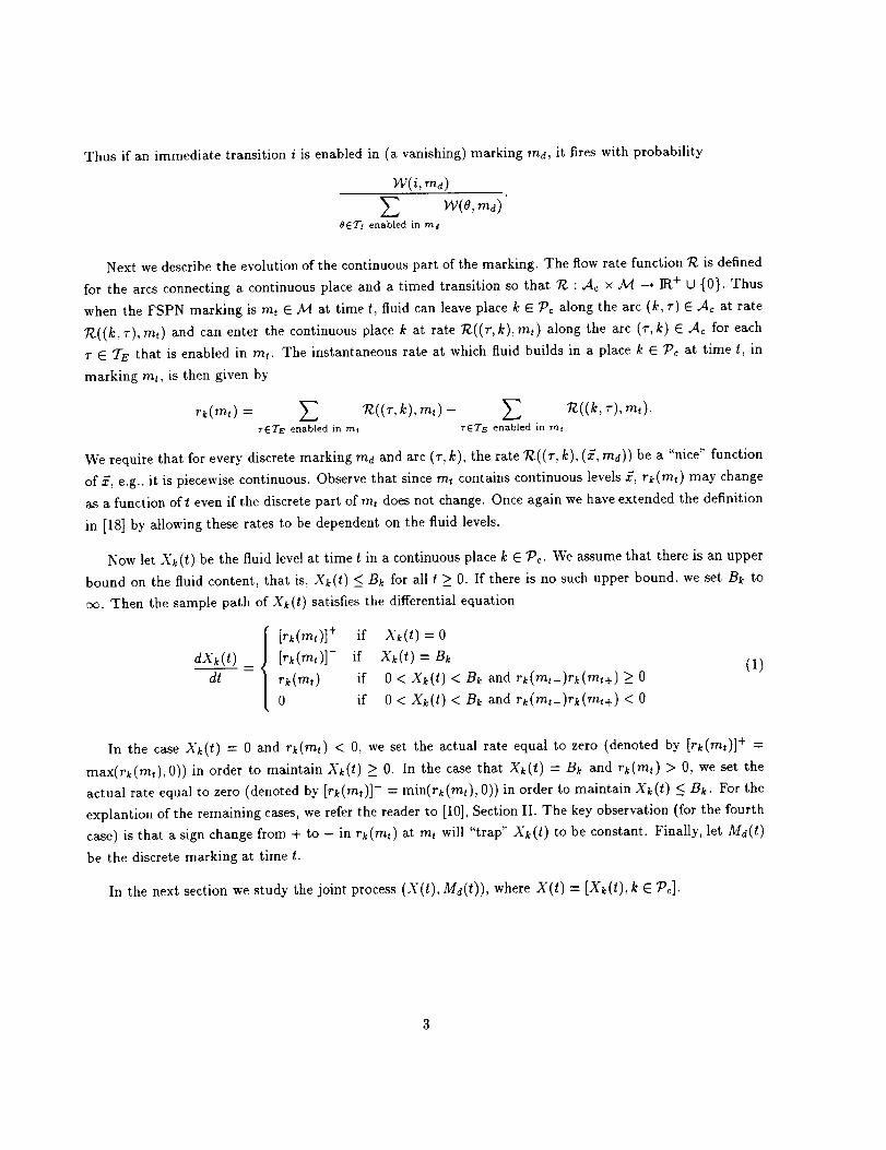
Thusif animmediatetransitioni is enabled in (a vanishing) marking rod, it fires with probability

14;(i, ma )

Z w(o, md)OfiT1 enabled in me

Next we describe the evolution of the continuous part of the marking. The flow rate function T¢ is defined

for the arcs connecting a continuous place and a timed transition so that T¢ : .Ac × A4 --* IR+ tO{0}. Thus

when the FSPN marking is rn, E Ad at time t, fluid can leave place k E 7_c along the arc (k, r) E .Ac at rate

7¢((k, r), mr) and can enter the continuous place k at rate T_((r, k), mr) along the arc (r, k) E Ac for each

v E 5rE that is enabled in mr. The instantaneous rate at which fluid builds in a place k E Pc at time t, in

marking m,, is then given by

rk(mt) = Z TC((r, k), mr) - _ 7¢((k, r), rn,).rETE enabled in rnt fETE enabled in rnt

We require that for every discrete marking md and arc (r, k), the rate TC((r, k), (£, rod)) be a "nice" function

of _, e.g., it is piecewise continuous. Observe that since rn, contains continuous levels aT, rk(mt) may change

as a function of t even if the discrete part of rnt does not change. Once again we have extended the definition

in [18] by allowing these rates to be dependent on the fluid levels.

Now let Xk(t) be the fluid level at time t in a continuous place k E Pc. We assume that there is an upper

bound on the fluid content, that is, Xk(t) <_ Bk for all t _> 0. If there is no such upper bound we set Bk to

o_. Then the sample path of Xk(t) satisfies the differential equation

[rk(m,)] if Xk(t)=O

dX_(t) _ [rk(rnt)]- if X_(I) = Bk

dt rk(mt) if 0 < Xk(t) < Bk and rk(m,-)rk(mt+ ) >_ 0

0 if 0 < Xk(t) < Bk and rk(mt-)rk(m_+) < 0

(1)

In the case Xk(t) = 0 and rk(mt) < 0, we set the actual rate equal to zero (denoted by [rk(mt)] + =

max(rk(mt),0)) in order to maintain Xk(t) >_ O. In the case that Xk(t) = Bk and rk(rnt) > 0, we set the

actual rate equal to zero (denoted by [rk(mt)]- = min(rk(mt), 0)) in order to maintain X_(t) < Bk. For the

explantion of the remaining cases, we refer the reader to [10], Section II. The key observation (for the fourth

case) is that a sign change from + to - in rk(mt) at mt will "trap" Xk(t) to be constant. Finally, let Md(I)

be the discrete marking at time t.

In the next section we study the joint process (X(t), Ma(t)), where X(t) = [X_(/), k E 7_¢].

3

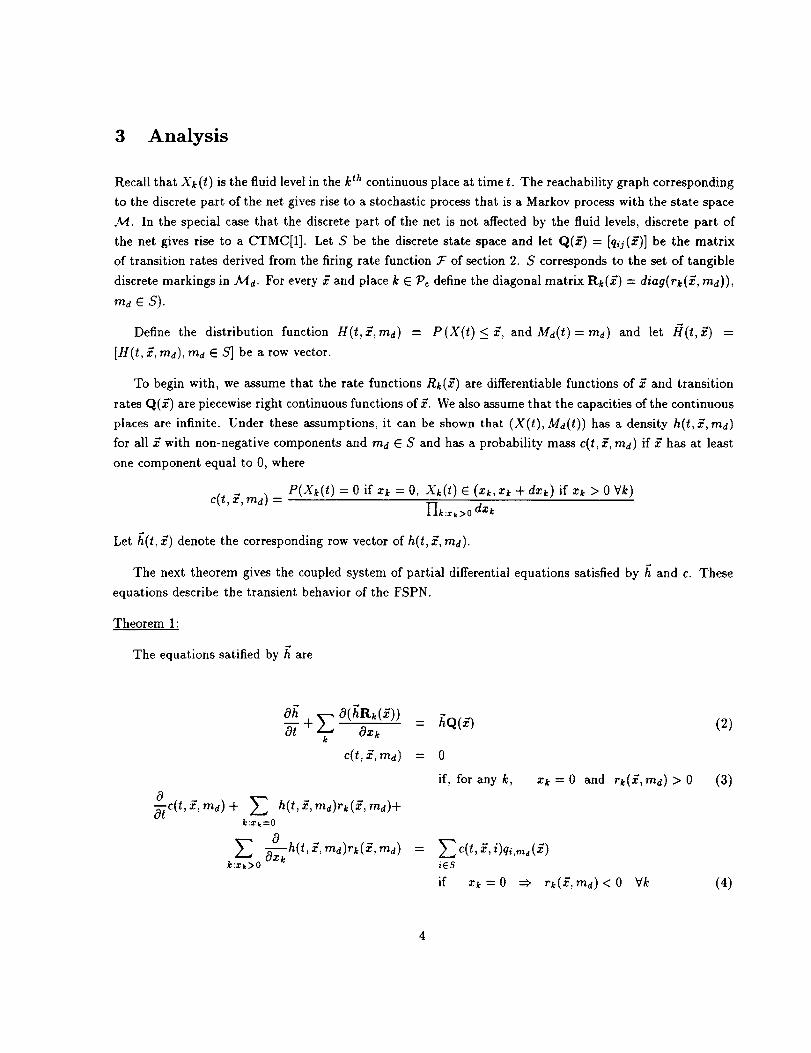
3 Analysis

Recall that Xk(t) is the fluid level in the k th continuous place at time t. The reachability graph corresponding

to the discrete part of the net gives rise to a stochastic process that is a Markov process with the state space

J_4. In the special case that the discrete part of the net is not affected by the fluid levels, discrete part of

the net gives rise to a CTMC[1]. Let S be the discrete state space and let Q(g) = [qq(g)] be the matrix

of transition rates derived from the firing rate function _- of section 2. S corresponds to the set of tangible

discrete markings in .h4d. For every _ and place k E Pc define the diagonal matrix Rk(£) = diag(rk(_, rod)),

md _ S).

Define the distribution function g(t,_,ma) = P(X(t) <_ _, and Ma(t) = ma) and let /_(t,_) =

[g(t, _,, ran), rnd E S] be a row vector.

To begin with, we assume that the rate functions Rk(_) are differentiable functions of g and transition

rates Q(_) are piecewise right continuous functions of g. We also assume that the capacities of the continuous

places are infinite. Under these assumptions, it can be shown that (X(t), Md(t)) has a density h(t, _, rna)

for all _ with non-negative components and md E S and has a probability mass c(t, _, rod) if _ has at least

one component equal to 0, where

e(t,_,md) = P(Xk(t) = 0 if zk = O, Xk(t) E (Zk,Xk +dzk) if zk > 0 Vk)l%: k>o

Let f_(t, 3) denote the corresponding row vector of h(t, _, rod).

The next theorem gives the coupled system of partial differential equations satisfied by f_ and c. These

equations describe the transient behavior of the FSPN.

Theorem 1:

The equations satified by f_ are

off O(fiRk(i))

k

c(t, ,rna) = 0

if, for any k,

=d) + h(t, ,'r,,,)+k:_k=0

__, _--_kh(t, _, md)rk(_, rnd)k:xa,>O

(2)

Z c(t, _, i)qi,m, (z)iES

if zk=0 ==_ r_(_,rnd)<0 vk (4)

xk=O and rk(_,md) >0 (3)

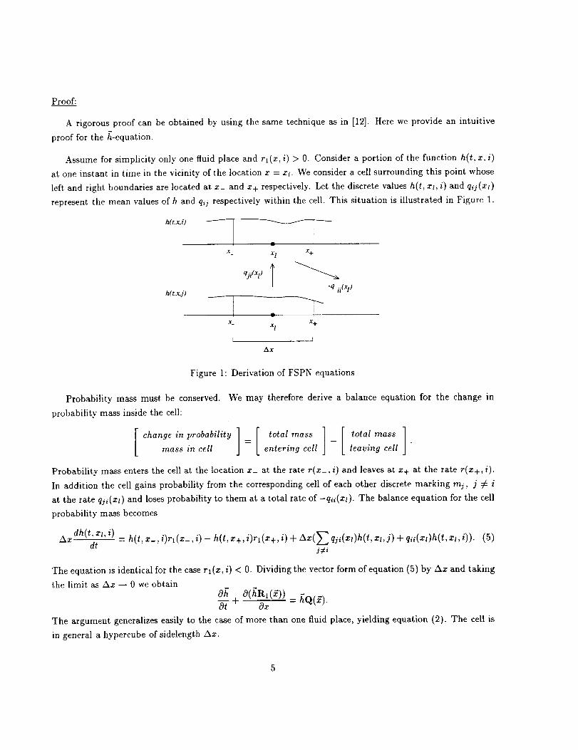
Proof:

A rigorousproofcanbeobtainedbyusingthesametechniqueasin [12].Hereweprovideanintuitiveprooffor theh-equation.

Assume for simplicity only one fluid place and rl(x, i) > O. Consider a portion of the function h(t, x, i)

at one instant in time in the vicinity of the location x = xt. We consider a cell surrounding this point whose

left and right boundaries are located at z_ and x+ respectively. Let the discrete values h(t, xt, i) and qij(xl)

represent the mean values of h and qij respectively within the cell. This situation is illustrated in Figure 1.

h(t.x,i)

h(t,x,j)

x Xl x+

"q ii(Xl)

x Xl x+

I I

Ax

Figure 1: Derivation of FSPN equations

Probability mass must be conserved.

probability mass inside the cell:

change in probabilitymass in cell

We may therefore derive a balance equation for the change in

--- m .

entering cell leaving cell

Probability mass enters the cell at the location z_ at the rate r(x_, i) and leaves at x+ at the rate r(z+, i).

In addition the cell gains probability from the corresponding cell of each other discrete marking mj, j _ i

at the rate q/i(zt) and loses probability to them at a total rate of -qii(xz). The balance equation for the cell

probability mass becomes

Axdh(t, xt, i) _ h(t, z_, i)rl(x_, i) - h(t, z+, i)rx(z+, i) + Ax(_-_ qji(xz)h(t, xt,j) + qii(zl)h(t, zt, i)). (5)dt j_i

The equation is identical for the case rl (z, i) < 0. Dividing the vector form of equation (5) by Ax and taking

the limit as Az _ 0 we obtainof_ 0(f_Rl(i))o--7+ -

The argument generalizes easily to the case of more than one fluid place, yielding equation (2). The cell is

in general a hypercube of sidelength Ax.

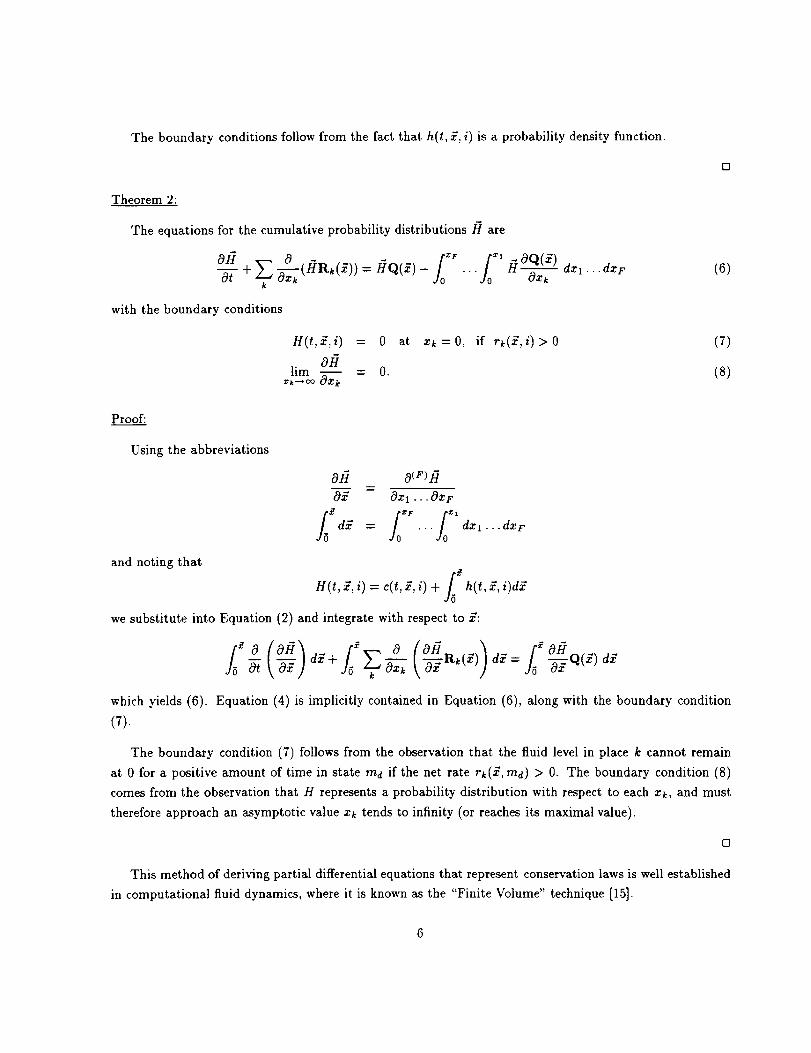
The boundary conditions follow from the fact that h(t, £, i) is a probability density function.

[2

Theorem 2:

The equations for the cumulative probability distributions/7 are

0H0--T _(/7R_(£)) f0 _F f_/7 0Q(£)+ V =/7Q(£)- ... dxl...dxr

with the boundary conditions

H(t,£,i) = 0 at xk=O, if rk(£,i)>O

0#lim - O.

xk_oO 0X k

(6)

(7)

(8)

Proof:

Using the abbreviations

and noting that

o/7 0(r)/70£ Oxl ... OxF

H(t, £, i) = c(t, £, i) + h(t, £, i)d£

we substitute into Equation (2) and integrate with respect to £:

;o o(o )_ d£+. V_-zk -_-Rk(£) d£= --_Q(g) d£

which yields (6). Equation (4) is implicitly contained in Equation (6), along with the boundary condition

(7).

The boundary condition (7) follows from the observation that the fluid level in place k cannot remain

at 0 for a positive amount of time in state ma if the net rate rk(£, md) > 0. The boundary condition (8)

comes from the observation that H represents a probability distribution with respect to each xk, and must

therefore approach an asymptotic value xk tends to infinity (or reaches its maximal value).

o

This method of deriving partial differential equations that represent conservation laws is well established

in computational fluid dynamics, where it is known as the "Finite Volume" technique [15].

TheassumptionsonRk(_')canbe relaxedandwecanallowRk(Z)to bepiecewisedifferentiableandfluid placesto havefinitecapacities.Thismayintroducenon-zeroprobabilitymassesat the inter-regionboundariesandwillneedto beexplicitlyaccountedfor.

Thedomainof Equations(2)and(6) is

0< xk < Bk

0< t <co,

although in practice we will only be interested in the finite domain 0 < t < tmax, 0 < zk < min{xmaz, Bk}

(where xmax is finite when Bk = oc).

The initial conditions for Equation (6) are

H(0, Z,i) = 1 if i=md0and_>__0

H(0,£,i) = 0 otherwise.

The initial conditions for Equation (2) are

e(O, _, i) = 6(too)

where/5 is the delta function.

Now suppose the following limits exist

f(_) = lira/-7(t, _)._---* OO

Then from Theorem 2, we see that the steady-state distribution f(_) obeys the following system of differential

equations

0 [ _OQ(_) d_, (9)

k

normalization condition lim f(_)g= 1, where gis a column vector of all l's.with the_oo

We note that the steady-state distribution f exists when

lim ZTri(_)rk(g'i)<0 k=l...FSk_OO

i

where 7r(f) is the solution of

.(_)q(_) = o

_ri(_) = 1

3.1 FSPN with a Single Continuous Place

In the special case of a single continuous place, Equation (9) reduces to:

(f(x)R(x)) = f(x)q(z)- Oz

In the following subsections, we consider three special cases of the Equation (10).

(10)

3.1.1 Constant Case

In the special case that R(x) and Q(x) are both independent of x, following [3], solution of such an equation

is of the form f(x) = he _ where h is a row vector and A is a scalar. Substituting in (10) we have

h(AR- Q) -- 0. (11)

If a non-zero h is to satisfy the above equation, we must have det(AR-Q) = 0. The number of solutions

of det(AR-Q) = 0 equals the number of non-zero diagonal elements of R(x). Let these solutions be denoted

by A1, A2.-., Ak. Let f_i be the solution to hi(AiR - Q) = 0. Then the general solution to (10) is given by

k

F(x) = E aif_ie;_'_: (12)i=1

where the scalars ai need to be determined from the boundary conditions and the boundedness of F(x). It

is known that the number of Ai's with positive real part equals the number of negative diagonal entries of

R. The coefficient ai corresponding to an eigenvalue Ai with Re(Ai) > 0 must be zero in order to maintain

boundedness of f(x). The remaining coefficients ai are uniquely determined by the boundary condition

F(0, m) = 0 if r(m) > 0.

Now if R(x) and Q(x) are both piecewise constant functions of x, we can apply the above procedure

for each different segment and piece the individual solutions together [10]. In the general case, we can use

numerical solution methods for linear odes that are available. We refer here to explicit methods such as

RKF-45 or implicit methods such as implicit Runge-Kutta [4] or TR-BDF2 [5] and so on.

4 Examples

Next we examine a number of examples to illustrate the modeling power of FSPNs.

# P2 2 L(#p

l f2 # Pl ,#P2 ,x)

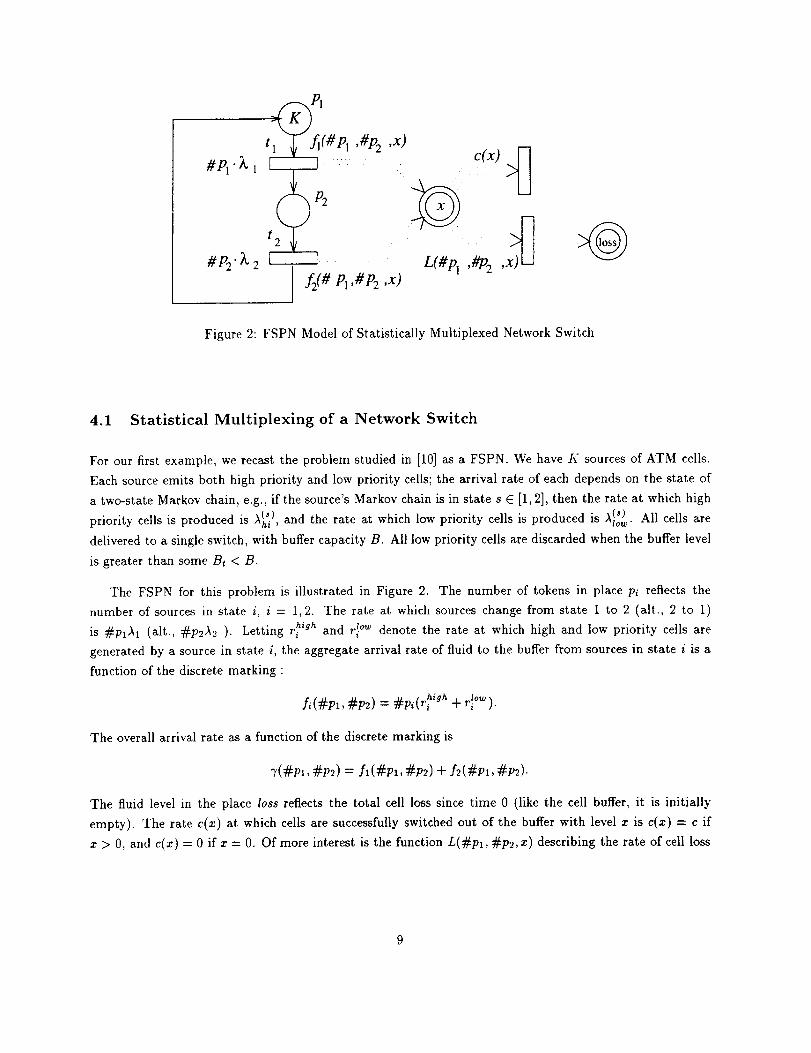
Figure 2: FSPN Model of Statistically Multiplexed Network Switch

4.1 Statistical Multiplexing of a Network Switch

For our first example, we recast the problem studied in [10] as a FSPN. We have K sources of ATM cells.

Each source emits both high priority and low priority cells; the arrival rate of each depends on the state of

a two-state Markov chain, e.g., if the source's Markov chain is in state s E [1, 2], then the rate at which high

x(*) All cells arepriority cells is produced is x(_) and the rate at which low priority cells is produced is "'Io,_"'hi _

delivered to a single switch, with buffer capacity B. All low priority cells are discarded when the buffer level

is greater than some Bt < B.

The FSPN for this problem is illustrated in Figure 2. The number of tokens in place Pi reflects the

number of sources in state i, i = 1,2. The rate at which sources change from state 1 to 2 (alt., 2 to 1)

Zow denote the rate at which high and low priority cells areis #p1A1 (alt., #p2A2 ). Letting rhigh and r i

generated by a source in state i, the aggregate arrival rate of fluid to the buffer from sources in state i is a

function of the discrete marking :

k(#pl, #p2) = #vi(r igh+

The overall arrival rate as a function of the discrete marking is

"r(#p_, #p2) = k(#pl, #p2) + I2(#p_, #p2).

The fluid level in the place loss reflects the total cell loss since time 0 (like the cell buffer, it is initially

empty). The rate c(x) at which cells are successfully switched out of the buffer with level x is c(z) = c if

x > 0, and c(z) = 0 if x = 0. Of more interest is the function L(#pl, #p_, x) describing the rate of cell loss

:: talways @<r::

(Pd

t F

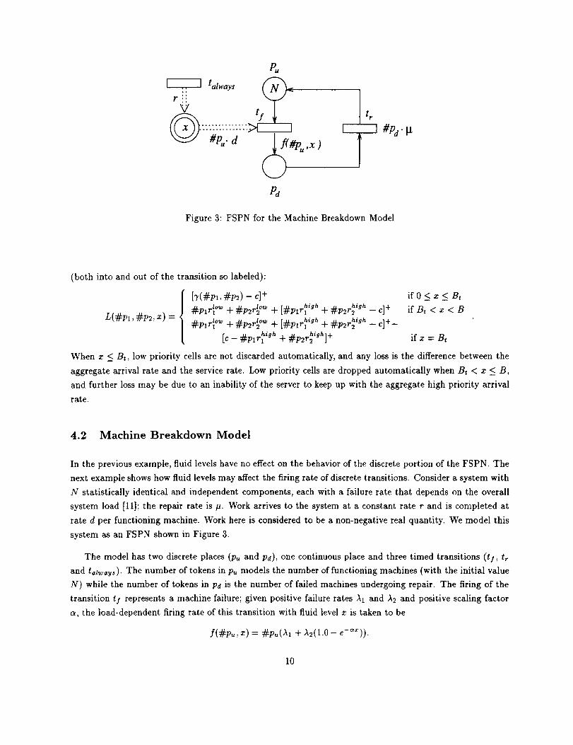
Figure 3: FSPN for the Machine Breakdown Model

(both into and out of the transition so labeled):

[7(#Pl, #p_) - el + if 0 < x < Bt

f..t£_ high ..u._ high#Ptr_ °w + _P2r_ °w + t-#-tq"l + _-e2,_ -- c]+ if Bt < x < B

L( #pl , #p_, X)_t__ high+ + + - d+-

• . high1+[c- #pl rhzgh + _p2r 2 J if z = Bt

When x < Bt, low priority cells are not discarded automatically, and any loss is the difference between the

aggregate arrival rate and the service rate. Low priority cells are dropped automatically when B_ < x < B,

and further loss may be due to an inability of the server to keep up with the aggregate high priority arrival

rate.

4.2 Machine Breakdown Model

In the previous example, fluid levels have no effect on the behavior of the discrete portion of the FSPN. The

next example shows how fluid levels may affect the firing rate of discrete transitions. Consider a system with

N statistically identical and independent components, each with a failure rate that depends on the overall

system load [11]; the repair rate is #. Work arrives to the system at a constant rate r and is completed at

rate d per functioning machine. Work here is considered to be a non-negative real quantity. We model this

system as an FSPN shown in Figure 3.

The model has two discrete places (p= and Pa), one continuous place and three timed transitions (t], tr

and tatways). The number of tokens in Pu models the number of functioning machines (with the initial value

N) while the number of tokens in Pa is the number of failed machines undergoing repair. The firing of the

transition tf represents a machine failure; given positive failure rates A1 and A2 and positive scaling factor

c_, the load-dependent firing rate of this transition with fluid level x is taken to be

f(#pu,x) = #pu(A1 + A2(1.0- e-at)).

10

Off

rhighf_X_ _- " 1

_' ===) _J)/======- _'high

Onlow

r,ow -:;::-->1 ,ow

high (_

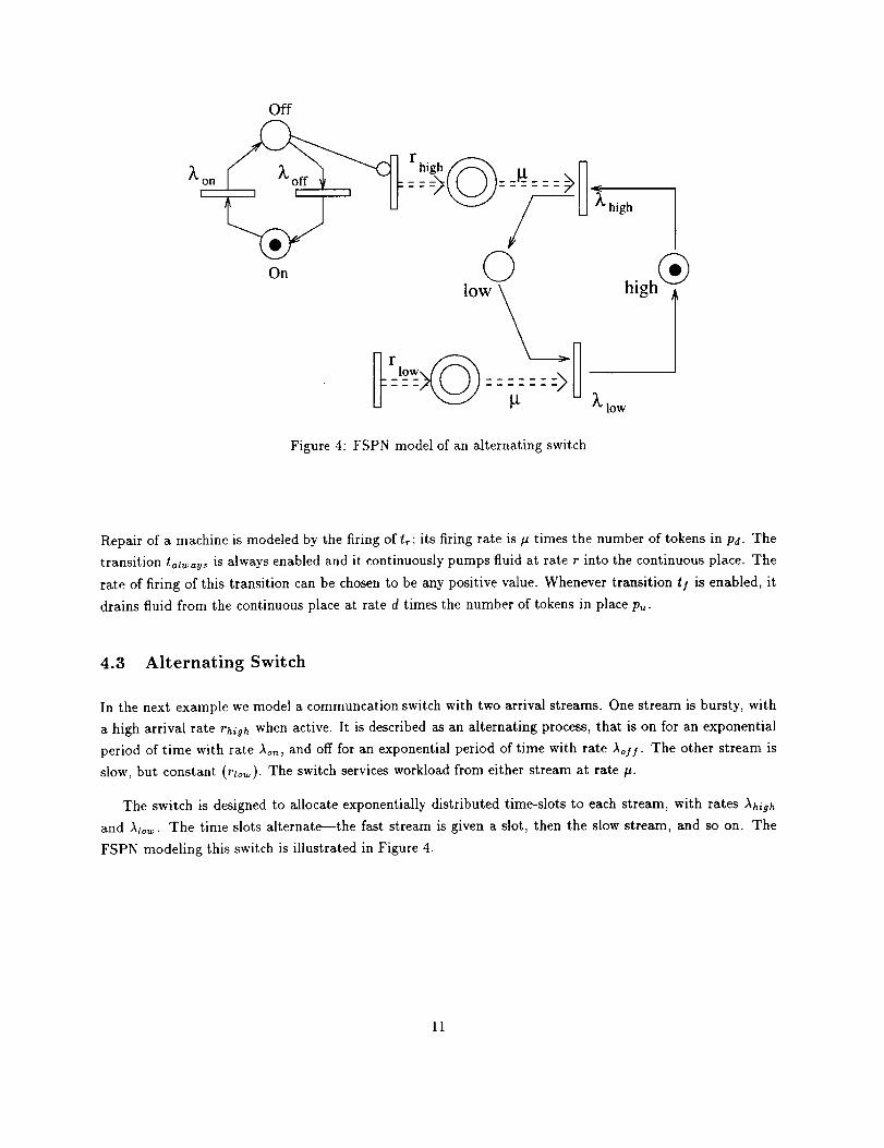
Figure 4: FSPN model of an alternating switch

Repair of a machine is modeled by the firing of tr; its firing rate is/_ times the number of tokens in Pd. The

transition taJway._ is always enabled and it continuously pumps fluid at rate r into the continuous place. The

rate of firing of this transition can be chosen to be any positive value. Whenever transition ty is enabled, it

drains fluid from the continuous place at rate d times the number of tokens in place p_.

4.3 Alternating Switch

In the next example we model a communcation switch with two arrival streams. One stream is bursty, with

a high arrival rate thigh when active. It is described as an alternating process, that is on for an exponential

period of time with rate Ao,_, and off for an exponential period of time with rate _oYl" The other stream is

slow, but constant (riot). The switch services workload from either stream at rate/_.

The switch is designed to allocate exponentially distributed time-slots to each stream, with rates ,_high

and )_to_. The time slots alternate--the fast stream is given a slot, then the slow stream, and so on. The

FSPN modeling this switch is illustrated in Figure 4.

11

5 Numerical Transient Analysis

5.1 Discretization

We choose to solve the equations for the probability distribution (6) rather than the density equations

(2), since the latter would require the numerical treatment of a delta function used to describe the initial

condition. We describe here the case R(£) = const, Q(£) = const.

We perform a semi-discretization of (6) in the coordinate directions zk, using a first-order upwind method.

In the nomenclature of section 3, the upwind scheme approximates values at the boundaries of the cell by

those at the neighbouring grid points in the upstream direction, relative to the flow direction r. We choose a

finite domain 0 < zk < xmax and use G equidistant grid points. The grid spacing (mesh size) Az is therefore

equal to xmax/(G- 1). Note that in order that the boundary condition (8) be approximately satisfied,

xrnax must be chosen to be sufficiently large. We use the notation r_,z_ ..... _F,i = rk(/1Ax,...,IFAx,i),

qi,jd, ..... IF = qii(llAx, ..., IFAx) and/Ii,h ..... Ir(_) = H(t, llAx,..., IFAx, i) . The upwind discretization is

given by

0 H(t,...,xk = lkAx,...,i) ,._ K-_ - (13)

cOzk _ [Hi,...,(,+0_,...(t) -/_i,...,z_,...(0) if rk ..... Ik..... i < 0

We obtain from the semi-discretization the linear system of ordinary differential equations

dt

where the unknown vector

(14)

is obtained by a lexicographic ordering of the unknowns by fluid place and by the discrete marking.

The matrix (_ is given by

(_ = (_+W

where (_ represents the CTMC of the discrete part of the net, and W the discretization of the space

QI1 • •. Q1M

QM1 ... QMM

derivatives multiplied by the flow rates.

The matrix (_ is given by

12

whereqij,01 ,...,OF

Qij = "..

qij,(G-1) ...... (G-l)r

Note that the matrix (_ is a CTMC matrix. The block-diagonal matrix W has the form

W __ ----

w_ o1

Az

0 WM

where Wi E IRaF×ar represents the discretization of the second term of equation (6) for the i-th discrete

marking using the upwind method (13). Each Wi is a sparse, banded matrix in which each column is either

zero or has a positive main diagonal coefficient and non-positive off-diagonal coefficients containing the rate

values ri ..... In addition, the main diagonal coefficient is the negative sum of the other entries in its column.

Each Wi, and thus also W, therefore represents the transpose of a CTMC.

The linear system of ordinary differential equations (14) thus defined may be integrated by any standard

method. In the numerical examples in section 6 we will use the Forward Euler scheme

H(t + A 0 _/{(0 + 5t/f(t)O.

Note that for this scheme the discretization mesh sizes must satisfy

in order that the integration be stable.

max rk,...,iAt < Ax (15)k,ll,.,.,lF,i

5.2 Numerical Integration in a Transformed Domain

In order to avoid the difficulty of solving equation (6) in an arbitrarily large and a priori unknown domain,

we can perform the coordinate transformation

y_ = 1 - e -_ (16)

which maps the infinite interval xk = [0, co] to the finite interval y_ = [0, 1]. Equation (6) then becomes

0t7(17)

+ _ - Yk) = fY/70Qd0---(

for/7(t, y-*). The boundary and initial conditions remain unchanged.

This minor modification to the equations makes their solution significantly easier, since the decision

where to place xmax must no longer be made, and the danger of an inappropriate choice is avoided. The

13

coordinatetransformationhastheadditionaladvantageof compressingtheinfiniteintervalof the largez

values, where in many cases the solution shows virtually no structure, into a small space. Furthermore,

we can obtain numerical values at z = oo, which correspond to the probabilities for the discrete markings,

whereas in the untransformed case these must be approximated by values obtained at z = xmax.

5.3 Problem Size

Recall that G denotes the number of gridpoints in each dimension zi, F the number of fluid places, and M

the number of discrete markings. The number of time-steps to be integrated is T.

The computational complexity for the solution is O(TMG r) floating point operations, since for each of

T timesteps we must increment each solution value in an F-dimensional grid of sidelength G for each of

M discrete markings using O(1) operations. Note that for an explicit integration method such as Forward

Euler, because the condition (15) must be satisfied, an increase in G must ultimately be accompanied by a

proportionate increase in T.

The storage requirements of the algorithm are at least 4MG F bytes since for each of M discrete markings

we must store an F-dimensional grid of floating point numbers with sidelength G. Solutions at successive

time-steps can be overwritten.

Since the sidelength of the grids G may typically be of the order of 50 or more when a simple discretization

is used, we see that this would seriously limit the size of the FSPNs that can be solved. Future work must

therefore include strategies for reducing the amount of memory needed to represent the function H.

5.4 Time Integration by Randomization

Randomization is a numerical method widely used for the solution of systems of ODEs of the form (14). It

has the advantages of high numerical stability and low roundoff error, a priori specification of absolute error

tolerance requirements, and is in addition often found to be faster than numerical integration schemes. The

method has superior roundoff error behavior when the matrix P = (I + _Q) has all non-negative entries,

where A > maxlQii [. This is, for example, the case for a CTMC.

As the following Theorem shows, the semi-discretized FSPN equation (14) also has this property, indi-

cating that randomization may be the method of choice for computing transient solutions.

Theorem 3:

For the matrix P = (I + _Q) where Q is the matrix of equation (14) holds

Pij >_ 0 Vi,j

14

H(UP) _._.__o.6 _" " " IIIIIIIII

o°._,_:.:_.._

0 """"

_'5_5o o.5 I I-5 2x 2.533.5

H(DOWN)

0.4 ,._o.3I . ,L mfllil/llh 0.2 ..::::.:.=.=::..

O. 1 L._,:._::_ •

i

3 3.5

6.5o o.5 _ _.5 _ _

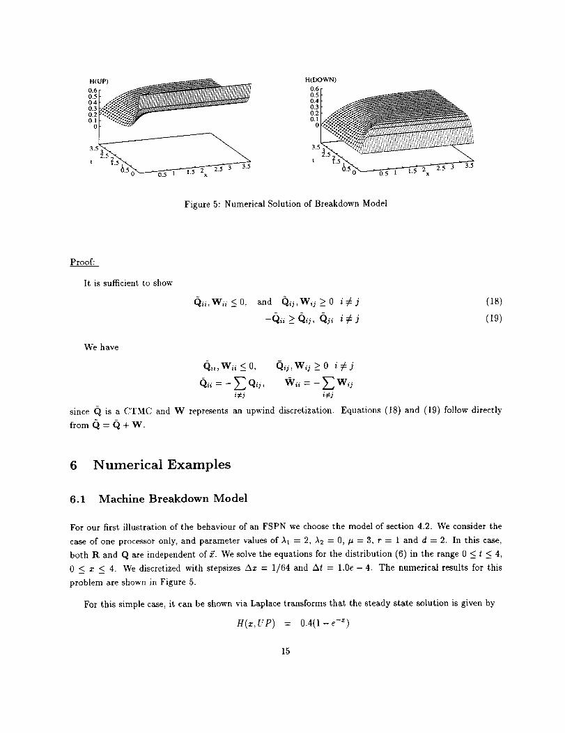
Figure 5: Numerical Solution of Breakdown Model

Proof:

It is sufficient to show

(_, Wii < 0, and (_ij,Wij_>0 i:_j

-Qii >_ qij, qji i# j

(18)

(19)

We have

Q;i, w. < 0,

since Q is a CTMC and W represents an upwind discretization.

fromQ=l_+W.

i#j

Equations (18) and (19) follow directly

6 Numerical Examples

6.1 Machine Breakdown Model

For our first illustration of the behaviour of an FSPN we choose the model of section 4.2. We consider the

case of one processor only, and parameter values ofAi = 2, A2 = 0, #=3, r= 1 and d=2. In this case,

both R and Q are independent of a?. We solve the equations for the distribution (6) in the range 0 < t < 4,

0 < x < 4. We discretized with stepsizes Ax = 1/64 and At = 1.0e - 4. The numerical results for this

problem are shown in Figure 5.

For this simple case, it can be shown via Laplace transforms that the steady state solution is given by

H(z, UP) = 0.4(1-e -z)

15

H(UP) ...... . .... "0.6 ,......o. l IIIIIIIII1 0.4 _/'_._,,._0:32 ..

t -'-_._

H(DOWN)

0.50.4 ' " "0.3

o.I°'2!_11:1i_1;o i,,,i_

3.5,, __

t "I'.5_

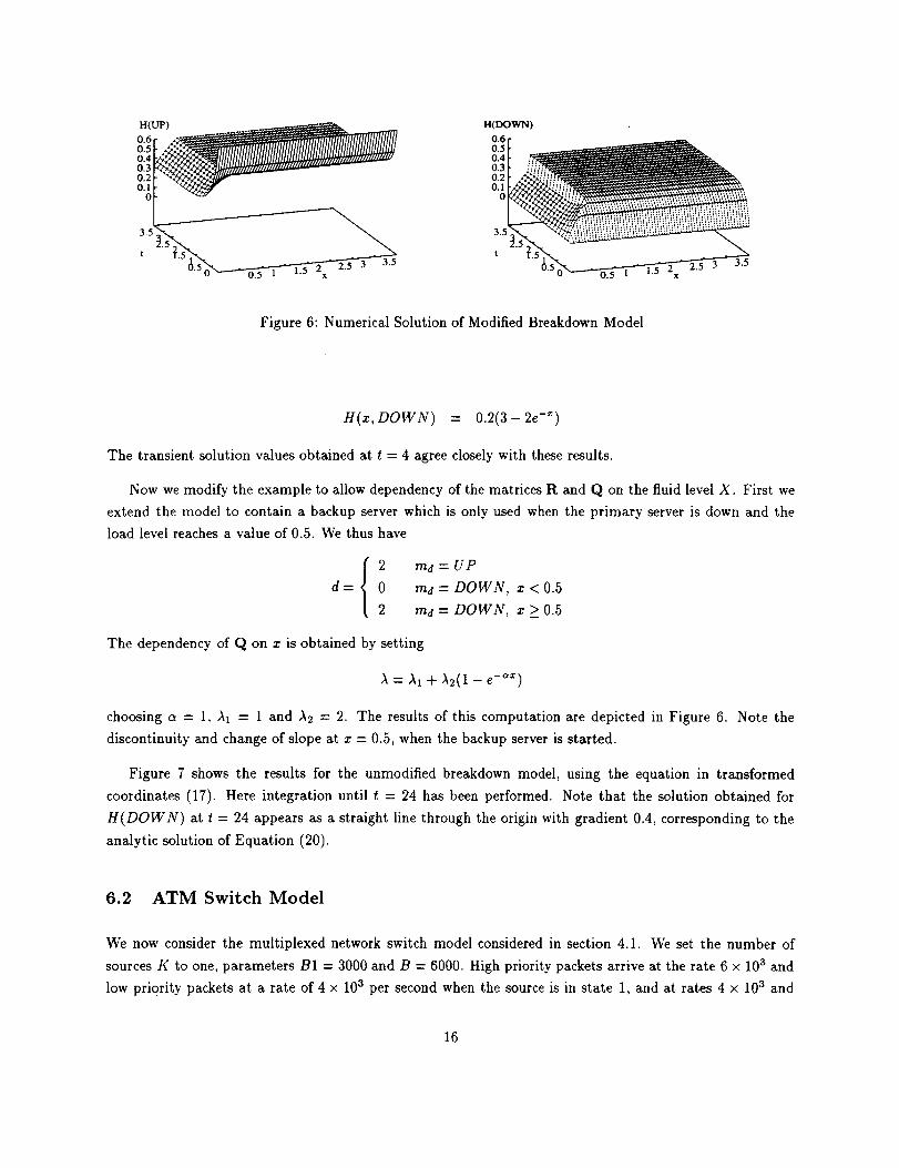
Figure 6: Numerical Solution of Modified Breakdown Model

H(x, DOWN) = 0.2(3- 2e -_)

The transient solution values obtained at t = 4 agree closely with these results.

Now we modify the example to allow dependency of the matrices R and Q on the fluid level X. First we

extend the model to contain a backup server which is only used when the primary server is down and the

load level reaches a value of 0.5. We thus have

2d= 0

2

md = UP

md = DOWN, x < 0.5

ma = DOWN, x > 0.5

The dependency of Q on x is obtained by setting

A = AI + A2(I - e -°_)

choosing (_ = 1, Az = 1 and A2 = 2. The results of this computation are depicted in Figure 6. Note the

discontinuity and change of slope at x - 0.5, when the backup server is started.

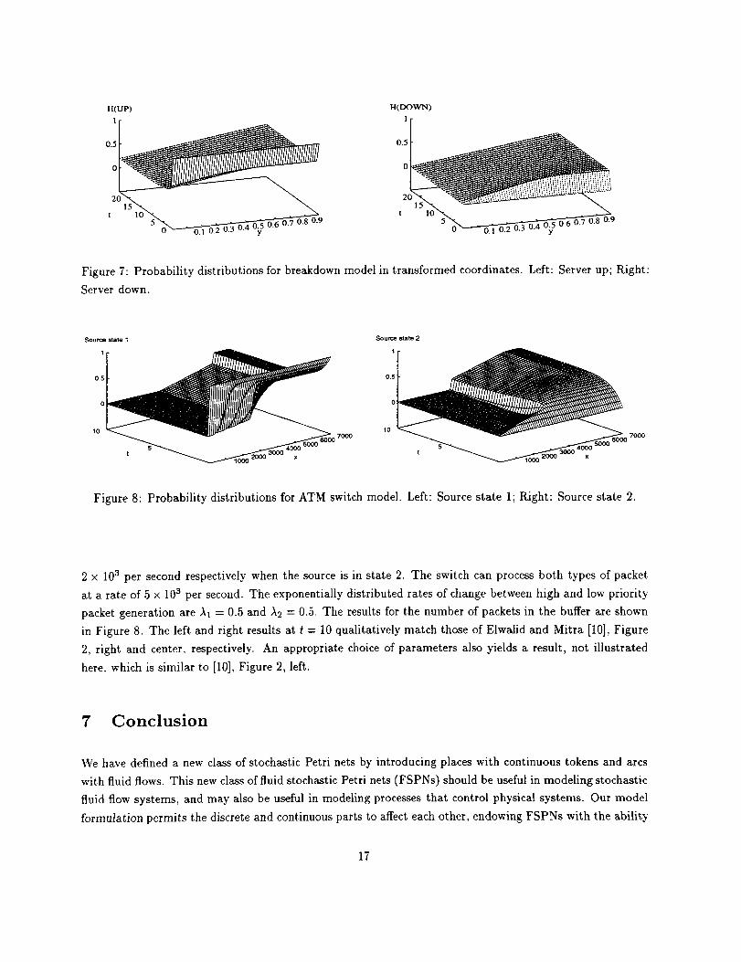
Figure 7 shows the results for the unmodified breakdown model, using the equation in transformed

coordinates (17). Here integration until t = 24 has been performed. Note that the solution obtained for

H(DOWN) at t = 24 appears as a straight line through the origin with gradient 0.4, corresponding to the

analytic solution of Equation (20).

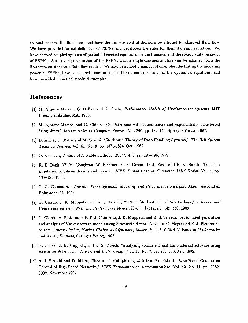
6.2 ATM Switch Model

We now consider the multiplexed network switch model considered in section 4.1. We set the number of

sources K to one, parameters B1 = 3000 and B = 6000. High priority packets arrive at the rate 6 × 10 a and

low priority packets at a rate of 4 x 10a per second when the source is in state 1, and at rates 4 × 10 3 and

16

H(UP)

o,°

10 _0.9

t 10

H(DOWN)

o.i5 _0.7 0.8 u._

Figure 7: Probability distributions for breakdown model in transformed coordinates. Left: Server up; Right:

Server down.

Source state 1

10 5 41300 5000 6000 7000

Source rote 2

10 7000

t

Figure 8: Probability distributions for ATM switch model. Left: Source state 1; Right: Source state 2.

2 x 103 per second respectively when the source is in state 2. The switch can process both types of packet

at a rate of 5 x 10 3 per second. The exponentially distributed rates of change between high and low priority

packet generation are _I = 0.5 and _2 = 0.5. The results for the number of packets in the buffer are shown

in Figure 8. The left and right results at t = 10 qualitatively match those of Elwalid and Mitra [10], Figure

2, right and center, respectively. An appropriate choice of parameters also yields a result, not illustrated

here, which is similar to [10], Figure 2, left.

7 Conclusion

We have defined a new class of stochastic Petri nets by introducing places with continuous tokens and arcs

with fluid flows. This new class of fluid stochastic Petri nets (FSPNs) should be useful in modeling stochastic

fluid flow systems, and may also be useful in modeling processes that control physical systems. Our model

formulation permits the discrete and continuous parts to affect each other, endowing FSPNs with the ability

17

to bothcontrolthefluid flow,andhavethediscretecontroldecisionsbeaffectedby observedfluid flow.Wehaveprovidedformaldefinitionof FSPNsanddevelopedtherulesfor their dynamicevolution.Wehavederivedcoupledsystemsofpartialdifferentialequationsforthetransientandthesteady-statebehaviorof FSPNs.Spectralrepresentationof theFSPNswith a singlecontinuousplacecanbeadaptedfromtheliteratureonstochasticfluidflowmodels.Wehavepresentedanumberofexamplesillustratingthemodelingpowerof FSPNs,haveconsideredissuesarisingin thenumericalsolutionof thedynamicalequations,andhaveprovidednumericallysolvedexamples.

References

[1] M. Ajmone Marsan, G. Balbo, and G. Conte, Performance Models of Multiprocessor Systems, MIT

Press, Cambridge, MA, 1986.

[2] M. Ajmone Marsala and G. Chiola, "On Petri nets with deterministic and exponentially distributed

firing times," Lecture Notes in Computer Science, Vol. 266, pp. 132-145. Springer-Verlag, 1987.

[3] D. Anick, D. Mitra and M. Sondhi, "Stochastic Theory of Data-Handling Systems," The Bell System

Technical Journal, Vol. 61, No. 8, pp. 1871-1894, Oct. 1982.

[4] O. Axelsson, A class of A-stable methods. BIT Vol. 9, pp. 185-199, 1969.

[5] R. E. Bank, W. M. Coughran, W. Fichtner, E. It. Grosse, D. J. Rose, and R. K. Smith, Transient

simulation of Silicon devices and circuits. IEEE Transactions on Computer-Aided Design Vol. 4, pp.

436-451, 1985.

[6] C. G. Cassandras, Discrete Event Systems: Modeling and Performance Analysis, Aksen Associates,

I-Iolmwood, IL, 1993.

[7] G. Ciardo, J. K. Muppala, and K. S. Trivedi, "SPNP: Stochastic Petri Net Package," International

Conference on Petri Nets and Performance Models, Kyoto, Japan, pp. 142-150, 1989.

[8] G. Ciardo, A. Blakemore, P. F. J. Chimento, J. K. Muppala, and K. S. Trivedi, "Automated generation

and analysis of Markov reward models using Stochastic Reward Nets," in C. Meyer and R. J. Plemmons,

editors, Linear Algebra, Markov Chains, and Queueing Models, Vol. 48 of IMA Volumes in Mathematics

and its Applications, Springer-Verlag, 1992.

[9] G. Ciardo, J. K. Muppala, and K. S. Trivedi, "Analyzing concurrent and fault-tolerant software using

stochastic Petri nets," J. Par. and Distr. Comp., Vol. 15, No. 3, pp. 255-269, July 1992.

[10] A. I. Elwalid and D. Mitra, "Statistical Multiplexing with Loss Priorities in Rate-Based Congestion

Control of IIigh-Speed Networks," IEEE Transaction on Communications, Vol. 42, No. 11, pp. 2989-

3002, November 1994.

18

[11]R. K. Iyer,D.J. RosettiandM. C. ttsueh,"MeasurementandModelingof ComputerReliabilityasAffectedbySystemActivity," ACM Transactions on Computer Systems, Vol. 4, pp. 214 - 237, August

1986.

[12] R. J. Karandikar and V. G. Kulkarni, "Second-order fluid flow models: Reflected Brownian motion in

a random environment," Operations Research, Vol. 43, No. 1, pp. 77-88, 1995.

[13] D. Mitra, "Stochastic Theory of Fluid Models of Multiple Failure-Susceptible Producers and Consumers

Coupled by a Buffer," Advances in Applied Probability, Vol. 20, pp. 646-676, 1988.

[14] T. Murata, "Petri Nets: Properties, analysis and applications," Proceedings of the IEEE, Vol. 77, No.

4, pp. 541-579, April 1989.

[15] S. V. Patankar, Numerical Heal Transfer and Fluid Flow, McGraw-Hill, New York, 1980.

[16] J. L. Peterson, Petri Net Theory and the Modeling of Systems, Prentice-Hall, Englewood Cliffs, N J,

USA, 1981.

[17] T. Robertazzi, Computer Networks and Systems: Queueing Theory and Performance Evaluation,

Springer-Verlag, 1990.

[18] K. S. Trivedi, V. G. Kulkarni, "FSPNs: Fluid Stochastic Petri Nets," Lecture Notes in Computer

Science, Vol 691, M. Ajmone Marsan (ed.), Proc. 14lh International Conference on Applications and

Theory of Petri Nets, Springer-Verlag, Heidelberg, pp. 24-31, 1993.

[19] N. Viswanadham and Y. Narahari, Performance Modeling of Automated Manufacturing Systems,

Prentice-Hall, Englewood Cliffs, N J, 1992.

19

Form ApprovedREPORT DOCUMENTATION PAGE OMBNo 0704-0188

Publicreporting burdenforthis collection of informationis estimatedto average1 hourperresponse,includingthe timefor revi_vinl[inStructionssearchingexistingdal_ sources.gather ngand maintaining the dataneeded andcompletingand reviewingthecollectionof information.Sendcommen_ regardingthis burdeneStimateor anyother aspectof thiscollection of information,includingsuggestionsfor reducingthisburden,to WashingtonHeadquartersServices.Directoratefor InformationOperations andReports,1215 JeffersonDavisHighway.Suite 1204, Arlington.VA 22202-4302,and to the Officeof Managementand Budget,PaperworkReductionProject(0704-0188).Washington,DC 2)0503,

]. AGENCY USE ONLY(Leave blank) 2. REPORT DATE

January 1996

4. TITLE AND SUBTITLE

FLUID STOCHASTIC PETRI NETS:THEORY, APPLICATIONS, AND SOLUTION

6. AUTHOR(S)

Graham Horton, Vidyadhar G. Kulkarni,

David M. Nicol, and Kishor S. Trivedi

7. PERFORMING ORGANIZATION NAME(S) AND ADDRESS(ES)

Institute for Computer Applications in Science and EngineeringMail Stop 132C, NASA Langley Research Center

Hampton, VA 23681-0001

9. SPONSORING/MONITORING AGENCY NAME(S) AND ADDRESS(ES)

National Aeronautics and Space Administration

Langley Research Center

Hampton, VA 23681-0001

3. REPORT TYPE AND DATES COVEREDContra£tor Report

5. FUNDING NUMBERS

C NAS1-19480

WU 505-90-52-01

8. PERFORMING ORGANIZATION

REPORT NUMBER

ICASE Report No. 96-5

10. SPONSORING/MONITORINGAGENCY REPORT NUMBER

NASA CR-198274ICASE Report No. 96-5

11. SUPPLEMENTARY NOTES

Langley Technical Monitor: Dennis M. BushnellFinal ReportSubmitted to the European Journal on Operations Research

12a. DISTRIBUTION/AVAILABILITY STATEMENT

U nclassified-U nlimited

Subject Category 60, 61

12b. DISTRIBUTION CODE

13. ABSTRACT (Maximum 200 words)In this paper we introduce a new class of stochastic Petri nets in which one or more places can hold fluid ratherthan discrete tokens. We define a class of fluid stochastic Petri nets in such a way that the discrete and continuousportions may affect each other. Following this definition we provide equations for their transient and steady-statebehavior. We present several examples showing the utility of the construct in communication network modelingand reliability analysis, and discuss important special cases. We then discuss numerical methods for computing thetransient behavior of such nets. Finally, some numerical examples are presented.

14. SUBJECT TERMS

Petri Nets; Performance Analysis; Reliability Analysis

17. SECURITY CLASSIFICATION 18. SECURITY CLASSIFICATION 19. SECURITY CLASSIFICATION

OF REPORT OF THIS PAGE OF ABSTRACT

Unclassified Unclassified

NSN 7540-01-280-5500

15. NUMBER OF PAGES

21

16. PRICE CODE

A0320. LIMITATION

OF ABSTRACT

Standard Form298(Rev. 249)Prescribed byANSI Std. Z39-18298-102