time misalignments in fault detection and diagnosis
TRANSCRIPT

TIME MISALIGNMENTS IN FAULT DETECTION AND DIAGNOSIS
David Alejandro LLANOS RODRÍGUEZ
ISBN: 978-84-691-8900-9 Dipòsit legal: GI-1593-2008

Universitat de Girona
Departament d’Electronica, Informatica i Automatica
Time Misalignments in
Fault Detection and Diagnosis
by
David Alejandro Llanos Rodrıguez
Advisors
Dr. Joaquim Melendez, Dr. Joan Colomer and Dr. Marcel Staroswiecki
DOCTORAL THESISGirona, SpainOctober, 2008

2
Universitat de Girona
Departament d’Electronica, Informatica i Automatica
Time Misalignments in
Fault Detection and Diagnosis
by
David Alejandro Llanos Rodrıguez
A dissertation presented to the Universitat deGirona in partial fulfillment of the requirementsof the degree of DOCTOR OF PHILOSOPHY
Advisors
Dr. Joaquim Melendez
Dr. Joan Colomer
Dr. Marcel Staroswiecki
Girona-Spain, October, 2008

3
Universitat de Girona
Departament d’Electronica, Informatica i Automatica
Abstract
Time Misalignments inFault Detection and Diagnosis
by David Alejandro Llanos Rodrıguez
Advisors: Dr. Joaquim Melendez, Dr. Joan Colomer and Dr. Marcel Staroswiecki
October, 2008Girona, Spain
The design of control, estimation or diagnosis algorithms most often assumes that allavailable process variables represent the system state at the same instant of time. How-ever, this is never true, because of the time misalignments. Time misalignment is theunmatching of two signals due to a distortion in the time axis of one or both signals.Potential sources of time misalignments are: different time response among sensors, datacommunication problems, analog to digital conversion, sensor location, and so on. FaultDetection and Diagnosis (FDD) deals with the timely detection, diagnosis and correctionof abnormal conditions of faults in a process. The methodology used in FDD is clearlydependent on the process and the sort of available information and it is divided in twocategories: model-based techniques and non-model based techniques. This doctoral dis-sertation deals with the study of time misalignments effects when performing FDD. Ourattention is focused on the analysis and design of FDD systems in case of data com-munication problems, such as data dropout and time delays due to data transmission.Techniques based on dynamic programming and optimisation are proposed to deal withthese problems. Numerical validation of the proposed methods is performed on differ-ent dynamic systems: a control position for a DC motor, a the laboratory plant and anelectrical system problem known as voltage sag.

4

Acknowledgments
I have had the privilege of working with three co-advisers. Dr. Joaquim Melendez and Dr.Joan Colomer who accepted me in eXiT (enginyeria de Control i Sistemes inTel·ligents),the research group that they have nurtured at the Univesitat de Girona. They bothshared with me their expertise in the field of Fault Detection and Diagnosis for which Iwould always be grateful. Their guidance during the structuring and development phasesof this thesis is also highly appreciated. Dr. Marcel Staroswiecki, from the University ofLille, offered me the opportunity of spending three months at the LAIL research group ofEcole Polytechnique Universitaire de Lille. The mathematical approach used in this thesiswas developed by Dr. Staroswiecki as well as the definition of the problem statement.I appreciate in particular, Dr. Staroswiecki encouragement and the high standard thathe demands as well as the promptness of his replies while editing this manuscript. Toall of them I am forever grateful as their mentoring and input to this work through ourdiscussions have contributed in shaping the way I approach scientific problems.
To the Universitat de Girona for the financial support through a research grant(BR01/01). Additionally, for the economical support during my 3 months as a visitor re-searcher at the LAIL research group of Ecole Polytechnique Universitaire de Lille, France.
This work has been partially supported by the projects “Desarrollo de un sistema decontrol y supervision aplicado a un reactor secuencial por cargas para la eliminacion demateria organica, nitrogeno y fosforo” (DPI2002-04579-C02-01) and DPI SECSE - “Su-pervision Experta de la Calidad de Servicio Electrico” (DPI2001-2198) within the CICYTprogram from the Spanish government and FEDER funds, which are hereby gratefullyacknowledged.
To the Universitat de Girona and to the company Sociedad de Explotacion de AguasResiduales S.A. -SEARSA-, for supporting me through the Agreement of EducationalCooperation (705/2005-06).
To my wife Rosa who with love and patience encouraged me during crucial momentsof my thesis. And overall, thanks for the so beautiful gift that you have given me, ourdaughter Paula, who is my Sun of every day.
To my parents Sebastian and Mariela who with their example, efforts and love makethe dreams of their children and grandchildren into reality. I would also like to expressmy gratitude to my siblings Flavio, Lyra, Ella, Rocıo and Jaime and my nieces Silvia,
5

6
Isabela and Alejandra. They all from distant places, but with the same unconditionalityand encouragement, were motivating me during this period.
To my family in Girona: Jose Maria, Paquita, Jordi, Maria and Julia, who have givenme great moments and make me feel like at home.
To the members of eXiT research group. Particular thanks to Francisco Gamero forsharing me the Time Warping Toolbox and for helping me with the development of theDTWon−line algorithm. I would also like to thank Juan Jose Mora and Magda Ruız fortheir collaboration in the field of Power Quality. I also want to mention a student whocontributed whit his work to the elaboration of some examples described in this work,this is the case of Xavier Berjaga. To all of them many thanks for their friendship andsupport during this time.
It is difficult to remember and to include every person who directly or indirectly hascollaborated in the development of this thesis. I offer my sincere apologies but I will everthank them.

Agradecimientos
He tenido el privilegio de haber trabajado con tres tutores. Dr. Joaquim Melendez y Dr.Joan Colomer los cuales me aceptaron en el grupo eXiT (ingenierıa de Control y SistemasinTeligentes), grupo de investigacion que dirigen en la Univesitat de Girona. Ambos hancompartido conmigo sus conocimientos en el campo de Deteccion y Diagnostico de Fallos,por lo cual les estare siempre agradecido. Su guıa durante la estructuracion y el desar-rollo de las diferentes fases de esta tesis es muy apreciada. Dr. Marcel Staroswiecki, del’Universite de Lille, me ofrecio la oportunidad de estar tres meses en el grupo de inves-tigacion LAIL de l’Ecole Polytechnique Universitaire de Lille, Francia. El procedimientomatematico y la definicion del problema han sido desarrollados por el Dr. Staroswiecki.Aprecio en particular los animos del Dr. Staroswiecki, el alto nivel y la inmediatez desus respuestas durante la edicion de este manuscrito. A todos ellos les estare siempreagradecido por sus aportaciones en este trabajo que han contribuido a mi formacion comoinvestigador.
A la Universitat de Girona por el soporte financiero con la beca de investigacion(BR01/01). Igualmente, por el soporte economico durante mis tres meses como investi-gador visitante en el grupo de investigacion LAIL de l’Ecole Polytechnique Universitairede Lille.
Este trabajo ha sido parcialmente apoyado por los proyectos “Desarrollo de un sistemade control y supervision aplicado a un reactor secuencial por cargas para la eliminacionde materia organica, nitrogeno y fosforo” (DPI2002-04579-C02-01) y DPI SECSE - “Su-pervision Experta de la Calidad de Servicio Electrico” (DPI2001-2198) dentro del CICYTprograma del gobierno Espanol y el fondo FEDER.
A la Universitat de Girona y a la empresa Sociedad de Explotacion de Aguas Resid-uales S.A. -SEARSA-, por su apoyo a traves del Convenio de Cooperacion Educativa num.705/2005-06.
A mi esposa Rosa quien con su amor y paciencia me ha animado en los momentoscruciales de mi tesis. Ademas, gracias por el maravilloso regalo que me ha dado, nuestrahija Paula, que es mi Solecito de cada dıa.
A mi padres Sebastian y Mariela quien con su ejemplo, esfuerzo y amor han hechorealidad los suenos de sus hijos y nietos. Tambien quiero expresar mi gratitud hacia mishermanos Flavio, Lyra, Ella, Rocıo y Jaime y mis sobrinas Silvia, Isabela y Alejandra.
7

8
Todos ellos desde sitios distantes, pero con la misma incondicionalidad y apoyo, me hanmotivado durante este perıodo.
A mi familia en Girona: Jose Maria, Paquita, Jordi, Maria y Julia, con los cuales hecompartido buenos momentos y me hacen sentir como en casa.
A los miembros del grupo de investigacion eXiT . Particularmente gracias a FranciscoGamero por compartir conmigo el “Time Warping Toolbox” y por ayudarme con el de-sarrollo del algoritmo DTWon−line. Quiero tambien dar las gracias a Juan Jose Mora yMagda Ruız por su colaboracion en el campo de Sistemas de Distribucion de EnergıaElectrica. Igualmente quiero mencionar a un estudiante que ha contribuido con su tra-bajo en la elaboracion de algunos ejemplos descritos en este trabajo, es el caso de XavierBerjaga. A todos ellos muchas gracias por su amistad y apoyo durante todo este tiempo.
Es difıcil recordar e incluir a todas las personas que directamente o indirectamentehan colaborado en el desarrollo de esta tesis. Ofrezco mis sinceras disculpas y al mismotiempo les doy las gracias.

Agraıments
He tingut el privilegi d’haver treballat amb tres tutors. Dr. Joaquim Melendez i Dr.Joan Colomer els quals em van acceptar al grup eXiT (enginyeria de Control i SistemesinTel·ligents), grup de recerca que dirigeixen a la Univesitat de Girona. Ambdos han com-partit amb mi els seus coneixements en el camp de Deteccio i Diagnosis de Falles, pel qualels estare sempre agraıt. La seva guia durant l’estructuracio i el desenvolupament de lesfases d’aquesta tesi es molt apreciada. Dr. Marcel Staroswiecki, de l’Universite de Lille,em va oferir l’oportunitat d’estar tres mesos al grup de recerca LAIL de l’Ecole Polytech-nique Universitaire de Lille, Franca. El procediment matematic i la definicio del problemaha estat desenvolupat pel Dr. Staroswiecki. Aprecio en particular l’encoratjament del Dr.Staroswiecki, l’alt nivell i la immediatesa de les seves respostes durant l’edicio d’aquestmanuscrit. A tots ells els estare sempre agraıt per les seves aportacions en aquest treballque han contribuıt a la meva formacio com a investigador.
A la Universitat de Girona pel suport financer amb la beca de recerca (BR01/01).Igualment, pel suport economic durant els meus tres mesos com a investigador visitant algrup de recerca LAIL de l’Ecole Polytechnique Universitaire de Lille.
Aquest treball ha estat parcialment recolzat pels projectes “Desarrollo de un sistemade control y supervision aplicado a un reactor secuencial por cargas para la eliminacionde materia organica, nitrogeno y fosforo” (DPI2002-04579-C02-01) i DPI SECSE - “Su-pervision Experta de la Calidad de Servicio Electrico” (DPI2001-2198) dins de CICYTprograma del govern Espanyol i el fons FEDER.
A la Universitat de Girona i a l’empresa Sociedad de Explotacion de Aguas Resid-uales S.A. -SEARSA-, pel seu suport a traves del Conveni de Cooperacio Educativa num.705/2005-06.
A la meva dona Rosa qui amb el seu amor i paciencia m’ha encoratjat en els momentscrucials de la meva tesi. I a mes, gracies pel meravellos regal que m’ha donat, la nostrafilla Paula, que es el meu Solet de cada dia.
Als meus pares Sebastian i Mariela qui amb el seu exemple, esforc i amor han fet re-alitat els somnis dels seus fills i nets. Tambe vull expressar la meva gratitud cap als meusgermans Flavio, Lyra, Ella, Rocıo i Jaime i les meves nebodes Silvia, Isabela i Alejandra.Tots ells des de llocs distants, pero amb la mateixa incondicionalitat i encoratjament,m’han motivat durant aquest perıode.
9

10
A la meva famılia a Girona: Jose Maria, Paquita, Jordi, Maria i Julia, amb els qualshe compartit bons moments i em fan sentir com a casa.
Als membres del grup de recerca eXiT . Particularment gracies a Francisco Gameroper compartir amb mi el “Time Warping Toolbox” i per ajudar-me amb el desenvolu-pament de l’algoritme DTWon−line. Vull tambe donar les gracies a Juan Jose Mora iMagda Ruız per la seva col·laboracio en el camp de Sistemes de Distribucio d’EnergiaElectrica. Igualment vull mencionar a un estudiant que ha contribuıt amb el seu treballen l’elaboracio d’alguns exemples descrits en aquest treball, es el cas de Xavier Berjaga.A tots ells moltes gracies per la seva amistat i suport durant tot aquest temps.
Es difıcil recordar i incloure a totes les persones que directament o indirectament hancol·laborat en el desenvolupament d’aquesta tesi. Ofereixo les meves sinceres disculpes ial mateix temps els dono les gracies.

Contents
Acknowledgments 5
Agradecimientos 7
Agraıments 9
Contents 11
List of Figures 15
List of Tables 17
1 Introduction 19
1.1 Motivation . . . . . . . . . . . . . . . . . . . . . . . . . . . . . . . . . . . . 19
1.2 Objectives . . . . . . . . . . . . . . . . . . . . . . . . . . . . . . . . . . . . 20
1.3 Thesis Outline . . . . . . . . . . . . . . . . . . . . . . . . . . . . . . . . . . 20
2 Fault Detection and Diagnosis 23
2.1 Introduction . . . . . . . . . . . . . . . . . . . . . . . . . . . . . . . . . . . 23
2.2 Terminology and definitions . . . . . . . . . . . . . . . . . . . . . . . . . . 23
2.2.1 Systems and controlled systems . . . . . . . . . . . . . . . . . . . . 25
2.2.2 Types of faults . . . . . . . . . . . . . . . . . . . . . . . . . . . . . 26
2.2.3 Approaches for fault detection and diagnosis . . . . . . . . . . . . . 27
2.3 Model-Based Techniques . . . . . . . . . . . . . . . . . . . . . . . . . . . . 27
2.3.1 Analytical redundancy for fault detection and isolation . . . . . . . 27
2.3.2 Fault detection and isolation techniques based on analytical models 31
2.3.3 Fault diagnosis based on qualitative-model . . . . . . . . . . . . . . 34
2.4 Non Model-Based Techniques . . . . . . . . . . . . . . . . . . . . . . . . . 34
2.4.1 Signal-based approaches . . . . . . . . . . . . . . . . . . . . . . . . 34
2.4.2 Knowledge-based approaches . . . . . . . . . . . . . . . . . . . . . . 35
2.5 Problems in Fault Detection and Diagnosis . . . . . . . . . . . . . . . . . . 37
2.5.1 Knowledge acquisition and representation . . . . . . . . . . . . . . 37
2.5.2 Measurement noise . . . . . . . . . . . . . . . . . . . . . . . . . . . 37
2.5.3 Modelling uncertainties . . . . . . . . . . . . . . . . . . . . . . . . . 38
2.5.4 Time misalignments . . . . . . . . . . . . . . . . . . . . . . . . . . 38
2.6 Conclusions . . . . . . . . . . . . . . . . . . . . . . . . . . . . . . . . . . . 41
11

12 CONTENTS
3 Time Misalignments in Supervisory Systems 433.1 Introduction . . . . . . . . . . . . . . . . . . . . . . . . . . . . . . . . . . . 433.2 Time Misalignments . . . . . . . . . . . . . . . . . . . . . . . . . . . . . . 44
3.2.1 Causes of time misalignments . . . . . . . . . . . . . . . . . . . . . 443.3 Modelling of Network Delays . . . . . . . . . . . . . . . . . . . . . . . . . . 47
3.3.1 Network modelled as constant delay . . . . . . . . . . . . . . . . . . 473.3.2 Network modelled as delays being independent . . . . . . . . . . . . 473.3.3 Network modelled using Markov chain . . . . . . . . . . . . . . . . 483.3.4 Network model adopted in this thesis . . . . . . . . . . . . . . . . . 48
3.4 Fault Diagnosis of Networked Control Systems . . . . . . . . . . . . . . . . 483.4.1 Delays in networked control systems . . . . . . . . . . . . . . . . . 483.4.2 Related works in Fault Diagnosis of Networked Control Systems . . 50
3.5 Time Misalignments in Residual Computation . . . . . . . . . . . . . . . . 533.5.1 Problem formulation . . . . . . . . . . . . . . . . . . . . . . . . . . 53
3.6 Time Misalignments in Signal Based Fault Diagnosis . . . . . . . . . . . . 563.6.1 Problem formulation . . . . . . . . . . . . . . . . . . . . . . . . . . 563.6.2 Previous work in signal comparison for fault diagnosis . . . . . . . 56
3.7 Conclusions . . . . . . . . . . . . . . . . . . . . . . . . . . . . . . . . . . . 59
4 Delay Estimation for Residual Computation 614.1 Introduction . . . . . . . . . . . . . . . . . . . . . . . . . . . . . . . . . . . 614.2 Influence of communications delays in residual computation . . . . . . . . . 614.3 The decision procedure under unknown transmission delays . . . . . . . . . 624.4 Estimating the transmission delays . . . . . . . . . . . . . . . . . . . . . . 63
4.4.1 Searching for a minimum . . . . . . . . . . . . . . . . . . . . . . . . 634.5 Application to a control position of a DC motor. . . . . . . . . . . . . . . . 68
4.5.1 Considering delays in one signal . . . . . . . . . . . . . . . . . . . . 694.5.2 Considering delays in two signals . . . . . . . . . . . . . . . . . . . 71
4.6 Conclusions . . . . . . . . . . . . . . . . . . . . . . . . . . . . . . . . . . . 75
5 Reduction of False Alarms in Fault Detection of Networked ControlSystems with Data Dropout 775.1 Introduction . . . . . . . . . . . . . . . . . . . . . . . . . . . . . . . . . . . 775.2 The influence of data dropout in residual computation . . . . . . . . . . . 785.3 Feasible residual computation . . . . . . . . . . . . . . . . . . . . . . . . . 78
5.3.1 The decision procedure under missing data . . . . . . . . . . . . . . 795.4 Illustrative example: Fault detection in a NCS laboratory plant . . . . . . 80
5.4.1 Description of the system . . . . . . . . . . . . . . . . . . . . . . . 805.4.2 Dropout communication model . . . . . . . . . . . . . . . . . . . . 825.4.3 Normal Operation . . . . . . . . . . . . . . . . . . . . . . . . . . . 83
5.5 Conclusions . . . . . . . . . . . . . . . . . . . . . . . . . . . . . . . . . . . 90
6 Dynamic Time Warping for Residual Computation 916.1 Introduction . . . . . . . . . . . . . . . . . . . . . . . . . . . . . . . . . . . 916.2 Dynamic Time Warping . . . . . . . . . . . . . . . . . . . . . . . . . . . . 926.3 On-line Dynamic Time Warping . . . . . . . . . . . . . . . . . . . . . . . . 95

CONTENTS 13
6.4 Dynamic Time Warping for improving Residual Computation in presenceof time misalignments . . . . . . . . . . . . . . . . . . . . . . . . . . . . . 98
6.5 Illustrative example: Fault detection in a NCS laboratory plant . . . . . . 996.5.1 Description of the system . . . . . . . . . . . . . . . . . . . . . . . 996.5.2 Results . . . . . . . . . . . . . . . . . . . . . . . . . . . . . . . . . . 1016.5.3 Time consuming . . . . . . . . . . . . . . . . . . . . . . . . . . . . 102
6.6 Conclusions . . . . . . . . . . . . . . . . . . . . . . . . . . . . . . . . . . . 103
7 Time Misalignment Reduction in Symptom Based Diagnosis 1057.1 Introduction . . . . . . . . . . . . . . . . . . . . . . . . . . . . . . . . . . . 1057.2 Case Based Reasoning . . . . . . . . . . . . . . . . . . . . . . . . . . . . . 1067.3 CBR cycle . . . . . . . . . . . . . . . . . . . . . . . . . . . . . . . . . . . . 107
7.3.1 Retrieval . . . . . . . . . . . . . . . . . . . . . . . . . . . . . . . . . 1077.3.2 Reuse . . . . . . . . . . . . . . . . . . . . . . . . . . . . . . . . . . 1097.3.3 Revise . . . . . . . . . . . . . . . . . . . . . . . . . . . . . . . . . . 1097.3.4 Retain . . . . . . . . . . . . . . . . . . . . . . . . . . . . . . . . . . 109
7.4 Effects of time misalignment in case retrieval . . . . . . . . . . . . . . . . . 1107.4.1 Cases represented as time-series and experience . . . . . . . . . . . 1107.4.2 Time misalignment in case retrieval . . . . . . . . . . . . . . . . . . 110
7.5 Dynamic time warping for case retrieval . . . . . . . . . . . . . . . . . . . 1117.6 Application in an Electrical System: diagnosis of voltage sags in a 25kV
substation . . . . . . . . . . . . . . . . . . . . . . . . . . . . . . . . . . . . 1117.6.1 Voltage sag definition . . . . . . . . . . . . . . . . . . . . . . . . . . 1117.6.2 Cases represented by voltage magnitude and location . . . . . . . . 1117.6.3 Dynamic Time Warping for voltage sag retrieval . . . . . . . . . . . 1127.6.4 Results . . . . . . . . . . . . . . . . . . . . . . . . . . . . . . . . . . 113
7.7 Conclusions . . . . . . . . . . . . . . . . . . . . . . . . . . . . . . . . . . . 116
8 Conclusions and Future Work 117
A Design of the analytical redundancy relation of a control position for aDC motor 121
B Design of the analytical redundancy relations of the laboratory plant 125
C Design of the analytical redundancy relations of the three tanks system127
D Temporal attributes of the voltage sags 131
Bibliography 135

14 CONTENTS

List of Figures
2.1 Time-dependency of faults: (a) abrupt; (b) incipient; (c) intermittent . . . 26
2.2 a) Structured residuals and b) Fixed-direction residuals . . . . . . . . . . . 30
2.3 (a) Bipartite graph G = (E ∪X,A′
) and complete matching of X into Eindicated by bold arcs. (b) RPG indicating that e5 is a redundant relation. 33
2.4 Data network delays in control systems . . . . . . . . . . . . . . . . . . . . 39
2.5 Two sequences that represent the measurements given by two sensors thatare measuring the same process variable. A) erroneous comparison due totime misalignment; B) intuitive alignment feature . . . . . . . . . . . . . . 40
3.1 1) Two similar time-series with the same mean and variance, 2) a possiblefeature alignment . . . . . . . . . . . . . . . . . . . . . . . . . . . . . . . . 44
3.2 Tank with and temperature sensor. The placement of the sensor will re-sult in an intrinsic time delay in measuring the tank fluid temperature,depending of the outflow rate . . . . . . . . . . . . . . . . . . . . . . . . . 46
3.3 Delays in NCS: communication delay between the sensor and the controller,τ sc; communication delay between the controller and the actuator, τ ca; andcomputational delay in the controller, τ c which could be included in τ ca,(Nilsson, 1988). . . . . . . . . . . . . . . . . . . . . . . . . . . . . . . . . . 49
3.4 Structure adopted in this thesis: the FDI unit of the NCS is placed in aremote node. . . . . . . . . . . . . . . . . . . . . . . . . . . . . . . . . . . 50
3.5 Data decomposition in distributed system . . . . . . . . . . . . . . . . . . 54
3.6 Two unsynchronised signals. a) erroneous comparison due to time mis-alignment; b) intuitive alignment feature . . . . . . . . . . . . . . . . . . . 57
4.1 Residual in fault free situation and comparison of actual and estimated delays 66
4.2 a)Level of significance, missed detections ( Type II error) and false alarms(Type I error). b)False minimisation without increasing the missed detec-tions. . . . . . . . . . . . . . . . . . . . . . . . . . . . . . . . . . . . . . . 67
4.3 Schematic diagram of a control position for a DC motor. . . . . . . . . . . 69
4.4 Block diagram of the system. . . . . . . . . . . . . . . . . . . . . . . . . . 70
4.5 Residual in fault free situation and comparison of actual and estimated delays 70
4.6 Cost function J(ρ(t)) . . . . . . . . . . . . . . . . . . . . . . . . . . . . . . 71
4.7 Residual in faulty situation and comparison of actual and estimated delays 72
4.8 Residual in fault free situation, comparisons of the actual and estimateddelays and the estimation error. . . . . . . . . . . . . . . . . . . . . . . . . 73
4.9 Cost function J(ρ(t)) . . . . . . . . . . . . . . . . . . . . . . . . . . . . . . 73
15

16 LIST OF FIGURES
4.10 Residual in faulty situation, comparisons of the actual and estimated delaysand the estimation error. . . . . . . . . . . . . . . . . . . . . . . . . . . . . 74
5.1 Laboratory plant . . . . . . . . . . . . . . . . . . . . . . . . . . . . . . . . 815.2 Process communication . . . . . . . . . . . . . . . . . . . . . . . . . . . . . 825.3 Residuals r1 and r2, tank level and input flow during normal situation. . . 845.4 Residuals r1 and r2 affected by data dropout on the sensor level. . . . . . . 855.5 Residuals ρ1 and ρ2 in presence of data dropout on the sensor level. . . . . 855.6 Residuals r1 and r2 affected by data dropout on the sensor level and a fault
on the flow-meter. . . . . . . . . . . . . . . . . . . . . . . . . . . . . . . . . 865.7 Residuals ρ1 and ρ2 during data dropout on the sensor level and a fault on
the flow-meter . . . . . . . . . . . . . . . . . . . . . . . . . . . . . . . . . . 865.8 Residuals r1 and r2 in presence of fault in the flow-meter and data dropout
in two sensors. . . . . . . . . . . . . . . . . . . . . . . . . . . . . . . . . . . 875.9 Residuals ρ1 and rρ2 in presence of fault in the flow-meter and data dropout
in two sensors. . . . . . . . . . . . . . . . . . . . . . . . . . . . . . . . . . . 885.10 FART (%) and theMDRT (%) of residuals r1(t) and ρ1(t) versus the dropout
rate. . . . . . . . . . . . . . . . . . . . . . . . . . . . . . . . . . . . . . . . 885.11 Relation between false alarms and missed detections as the λ parameter is
varied. . . . . . . . . . . . . . . . . . . . . . . . . . . . . . . . . . . . . . . 89
6.1 On-line DTW. . . . . . . . . . . . . . . . . . . . . . . . . . . . . . . . . . . 966.2 Laboratory plant . . . . . . . . . . . . . . . . . . . . . . . . . . . . . . . . 996.3 Process communication . . . . . . . . . . . . . . . . . . . . . . . . . . . . . 1006.4 Histograms of delays of the monitored process variables a)Ts=100ms b)Ts=1000ms.1016.5 a) r2 and b) ρ2 using DTWon−line. . . . . . . . . . . . . . . . . . . . . . . . 102
7.1 Cases and CBR cycle: Retrieve, Reuse, Retain and Revise. . . . . . . . . . 1087.2 a)Example of a three-phase voltage sag b) rms voltage . . . . . . . . . . . 1127.3 Voltage sag classification: a)Distribution b)Transmission. . . . . . . . . . . 1137.4 Two similar characteristic voltage sags. a) The Euclidean distance, b) DTW.1147.5 A wrong diagnosis of a new voltage sag. . . . . . . . . . . . . . . . . . . . 115
A.1 Schematic diagram of a control position for a DC motor. . . . . . . . . . . 121A.2 Oriented structure graph of the system . . . . . . . . . . . . . . . . . . . . 122
B.1 Oriented structure graph of the system. . . . . . . . . . . . . . . . . . . . . 126B.2 Image of the laboratory plant. . . . . . . . . . . . . . . . . . . . . . . . . . 126
C.1 Oriented structure graph of the three tanks system. . . . . . . . . . . . . . 128C.2 Image of the laboratory plant. . . . . . . . . . . . . . . . . . . . . . . . . . 129
D.1 Three-phase voltage sags attributes. . . . . . . . . . . . . . . . . . . . . . . 132D.2 Single-phase voltage sags attributes. . . . . . . . . . . . . . . . . . . . . . . 132D.3 Developed Tool for voltage sags registration . . . . . . . . . . . . . . . . . 134

List of Tables
2.1 Fault signature matrix. . . . . . . . . . . . . . . . . . . . . . . . . . . . . . 31
3.1 Typical time delays, (Trevelyan, 2004). . . . . . . . . . . . . . . . . . . . . 46
4.1 Decision thresholds for r(t) and ρ(t). . . . . . . . . . . . . . . . . . . . . . 684.2 Missed detection rate for r(t). . . . . . . . . . . . . . . . . . . . . . . . . . 694.3 Missed detection rate for ρ(t). . . . . . . . . . . . . . . . . . . . . . . . . . 69
5.1 False Alarm Ratio in T = [40, 80]s, when dropout occurs in one sensor . . . 845.2 False Alarm Ratio evaluated in T = [40, 80]s, when dropout occurs in two
sensors . . . . . . . . . . . . . . . . . . . . . . . . . . . . . . . . . . . . . . 87
6.1 A warping path in a m-by-n grid. . . . . . . . . . . . . . . . . . . . . . . . 926.2 The warping path is restricted in the grey area (the warping window). . . . 936.3 A cumulative distance matrix for sequences Q and S. . . . . . . . . . . . . 946.4 A cumulative distance matrix for sequences Q and S at the sample time
t = 3. . . . . . . . . . . . . . . . . . . . . . . . . . . . . . . . . . . . . . . . 966.5 Cumulative distance values of the sliding window for sequences Q and S
at time t = 4. . . . . . . . . . . . . . . . . . . . . . . . . . . . . . . . . . . 976.6 Cumulative distance values of the sliding window for sequences Q and S
at time t = 5. . . . . . . . . . . . . . . . . . . . . . . . . . . . . . . . . . . 976.7 Cumulative distance values of the sliding window for sequences Q and S
at time t = 6. . . . . . . . . . . . . . . . . . . . . . . . . . . . . . . . . . . 976.8 Time consuming comparison between DTW and DTWon−line . . . . . . . . 103
7.1 Diagnostic error using Euclidean, Manhattan and DTW distances . . . . . 114
A.1 Incidence matrix. . . . . . . . . . . . . . . . . . . . . . . . . . . . . . . . . 122
B.1 Incidence matrix. . . . . . . . . . . . . . . . . . . . . . . . . . . . . . . . . 126
C.1 Incidence matrix. . . . . . . . . . . . . . . . . . . . . . . . . . . . . . . . . 128
D.1 Reference values for temporal attributes normalisation. . . . . . . . . . . . 133
17

18 LIST OF TABLES

Chapter 1
Introduction
1.1 Motivation
Due to the growing complexity and spatial distribution of automated systems, commu-nication networks have become the backbone of most control architecture. As systemsare required to be more scalable and flexible, they have additional sensors, actuators andcontrollers, often referred to as field (intelligent) devices (Lee et al., 2001, Staroswiecki,2005). Networked Control Systems (NCS) result from connecting these system compo-nents via a communication network such as CAN (Controller Area Network), PROFIBUSor Ethernet. Control over data networks has many advantages compared with traditionalcontrol systems, such lower cost, greatly reduced wiring, weight and power, simpler instal-lation and maintenance and higher reliability. However, the design of control, estimationor diagnosis algorithms most often are affected by time misalignments. Time misalign-ment is the unmatching of two signals due to a distortion (expansion or compression) inthe time axis of one or both signals. Time misalignment can be produced by: differenttime response among sensors, analog to digital conversion, sensor location, data dropout,limited bandwidth, time delay due to data transmission, asynchronous clock among net-work nodes and other peculiarities of networks that could degrade the performances of theclosed-loop systems and even destabilize them. The aforementioned problems have beenintensively studied by the control community in the last several years (Zhang et al., 2001;Walsh and Hong, 2001; Walsh et al., 2002; Zhivoglydov and Middleton, 2003; Savkinand Petersen, 2003; Matveev and Savkin, 2003; Lian et al., 2003; Hu and Zhu, 2003; Maand Fang, 2005; Li and Fang, 2006), including: analysis of impact of network on controlperformance, design of control algorithm taking into account the above factors and pro-posal of new network protocol suitable for control. Nevertheless, only a few studies of theimpact of the communication network on the diagnosis of continuous systems have beenrecently published (Zhang et al., 2004; Ding and Zhang, 2005; Fang et al., 2006). Thechallenging problem that has motivated this thesis is the time misalignments effects whenperforming Fault Detection and Diagnosis (FDD).
19

20 1. Introduction
1.2 Objectives
In this thesis the problem of time misalignments when performing FDD is investigated.The main objective of the thesis is to design techniques aiming at the minimisation of falsealarms caused by transmission delay and data dropout without increasing the number ofmissed detection. The techniques rely on the explicit modelling of the communicationnetwork. Techniques based on dynamic programming and optimisation are proposed todeal with these problems. Numerical validation of the proposed methods is performed ondifferent dynamic systems: a control position for a DC motor, a the laboratory plant andan electrical system problem known as voltage sag.
1.3 Thesis Outline
The contents of the thesis are as follows:
Chapter 2: Fault Detection and Diagnosis
This chapter introduces the terminology used in the field of fault detection and diagnosis.An overview of various diagnostic methods from different perspectives is also provided.The general formulation that is used in next chapters and a discussion about problemsin fault detection and diagnosis are also presented. More emphasis has been put on timemisalignments which is the challenging problem that has motivated this thesis.
Chapter 3: Time Misalignments in Supervisory Systems
The concept of time misalignments is defined in this chapter and potential sources of timemisalignments are presented. Different models of network delays are given. The problemformulation of time misalignment and communication delays from model-based and nonmodel-based fault diagnosis perspectives are stated. The associated work done in bothdirections is also presented.
Chapter 4: Delay Estimation for Residual Computation
In this chapter, a technique aiming to the minimization of the false alarms caused bytransmission delays without increasing the number of missed detection is proposed. Thetechnique relies on the explicit modelling of communication delays, and their most likelyestimation. Application on a control position for a DC motor is shown.
Chapter 5: Reduction of False Alarms in Fault Detection of Net-worked Control Systems with Data Dropout
In this chapter, a technique aiming at the reduction of the false alarms caused by datadropout without increasing the number of missed detection is proposed. Illustrative ex-

1.3. Thesis Outline 21
ample on a laboratory plant is given.
Chapter 6: Dynamic Time Warping for Residual computation
This chapter proposes the use of Dynamic Time Warping (DTW) to reduce the effectsof time misalignment when residual computation is performed. The first section, Section6.2, summarises the DTW algorithm. In Section 6.3, a modification of DTW in orderto be applied on-line is explained. In Section 6.4 the use of DTW for improving theresidual computation in the presence of time misalignment is formulated. Finally, Section6.5 presents the applications in a laboratory plant of the University of Girona eXiT group.
Chapter 7: Time Misalignment Reduction in Symptom BasedDiagnosis
This chapter proposes the use of Dynamic Time Warping (DTW) for reducing the effectsof time misalignment when Case Based Reasoning (a symptom based diagnosis) is per-formed. DTW is used as a similarity criteria to implement the retrieval task. An electricalsystem problem, known as voltage sag, has been used to test the proposed method.
Chapter 8: Conclusions
In the last chapter conclusions are presented. Extensions and open problems are discussed.
Appendices
The thesis finishes with four appendices:
• A: Design of the analytical redundancy relation of a control position for a DC motor.
• B: Design of the analytical redundancy relations of the laboratory plant.
• C: Design of the analytical redundancy relations of the three tanks system.
• D: Temporal attributes of the voltage sags.

22 1. Introduction

Chapter 2
Fault Detection and Diagnosis
2.1 Introduction
Fault Detection and Diagnosis (FDD) deals with the timely detection, diagnosis and cor-rection of abnormal conditions of faults in a process. Early detection and diagnosis canhelp to avoid abnormal events progression and to reduce production loss. There is a wideliterature documentation on process fault diagnosis ranging from analytical methods toartificial intelligence and statistical approaches. From a modelling perspective, there aremethods that require accurate process models, semi-quantitative models or qualitativemodels. However, there are methods that do not assume any form of model informationand rely only on historic process data. Therefore, this chapter is mainly devoted to in-troduce the terminology used in the field of fault detection and diagnosis, to provide anoverview of various diagnostic methods from different perspectives, to introduce the gen-eral formulation that is used in next chapters and a discussion about drawbacks in faultdetection and diagnosis are also presented, doing more emphasis in time misalignmentswhich is the challenging problem that has motivated this thesis.
This chapter is organized as follows: Section 2.2 presents some terminologies anddefinitions that are used in the FDD field. Model-based techniques are gathered in Section2.3. In contrast, Section 2.4 explains the non model-based techniques. Problems in FDDare mentioned in Section 2.5. Finally some concluding remarks are given in Section 2.6.
2.2 Terminology and definitions
The terminology used in the field of fault detection and diagnosis is not unique. Conse-quently, the Safeprocess Technical Committee of IFAC (the International Federation ofAutomatic Control) compiled a list of suggested definitions (Isermann and Balle, 1997)which is in accordance with the terminology used this thesis.
23

24 2. Fault Detection and Diagnosis
About the states and the signals
• Fault : Unaccepted deviation of at least one characteristic property or parameter ofa system from its acceptable/usual/standard condition.
• Failure: inability of a system or a component to accomplish its function.
• False alarm: is an indication of a fault, when in actuality a fault has not occurred.
• Error : Deviation between a measured or computed value (of an output variable)and the true, specified, or theoretically correct value.
• Disturbance: An unknown (and uncontrolled) input acting on a system.
• Missed detection: when there is not indication of a fault, though a fault has occurred.
• Perturbation: An input acting on a system, which results in a temporary departurefrom the current estate.
• Residual : Fault information carrying signals, based on the deviation between mea-surements and the model based computations.
• Symptoms : A change of an observable quantity from its normal behaviour.
About the functions
• Fault detection: Determination of faults present in a system at a particular time.
• Fault isolation: Determination of the type, location, and time of detection of a fault.Follows fault detection.
• Fault diagnosis : Determination of the kind, size, location and time of occurrence ofa fault. Fault diagnosis includes fault detection, isolation and estimation.
• Monitoring : A continuous real-time task of determining the conditions of a phys-ical system, by recording information, recognising and indicating anomalies in thebehaviour.
• Residual computation: residual value is computed from the known variable.
• Residual evaluation: the residual is evaluated in order to detect, isolate and identifyfaults.
• Supervision: Monitoring of a physical system and taking appropriate actions tomaintain the operation in the presence of faults.

2.2. Terminology and definitions 25
About the models
• Qualitative model : A system model that describes the behaviour and relationshipsamong system variables and parameters in heuristic terms such as causalities of ifor then rules.
• Quantitative model : A system model that describes the behaviour and relationshipsamong system variables and parameters in analytical terms such as differential equa-tions.
• Diagnostic model : A set of static and dynamic relationships which link specific inputvariable -the symptoms- to specific output variables -the faults.
• Analytical redundancy : Use of two or more (but not necessary identical) ways todetermine a variable where one way uses a mathematical process model in analyticalform.
About the system properties and its measurements
• Reliability : Probability of a system to perform a required function under normalconditions and during a given period of time.
• Safety : Ability of a system not to cause any danger to people or equipment orenvironment.
2.2.1 Systems and controlled systems
A system is a set of interconnected components. Each of the components are chosen bythe system engineer for achieving some function of interest. A function describes whatthe design engineer expects the components to perform. A given component performsits task because it has been designed for exploiting some physical principle(s), which ingeneral are expressed by some relationship(s) between the evolution time of some systemvariables. Such relationships are called constraints, and the evolution time of the variablesis called trajectory.
Some of the components may have been selected with the aim of controlling the pro-cess, i.e, being able to choose, between all the possible system trajectories, the one whichwill bring some expected result (achieve some given objective). Those components whichallow to impose, or to influence, the trajectory of a given variable are called actuators.They establish some constraint between the variables of the process and some controlvariable, which is called control signal.
Actuators may be driven by human operators or by control algorithms. In both cases,closed loop control demands some information about the actual values of the systemvariables to be known. Sensors are components which are designed to provide this infor-mation. Thus a controlled systems is a set of interconnected components which includeprocess components, actuators, sensors and control algorithms.

26 2. Fault Detection and Diagnosis
f f
a
b
c
t t
Figure 2.1: Time-dependency of faults: (a) abrupt; (b) incipient; (c) intermittent
2.2.2 Types of faults
The types of faults depend basically on the their location within the system, the numberof components that can be affected and their temporal evolution.
Taking into account the effects of the faults, there are classified as additive faults (thosewhich correspond to sensor and actuator faults) and multiplicative faults (or parametric):
• Additive process faults : These are unknown inputs acting on the plant, which arenormally zero and which, when present, can cause a change in the plant outputsindependent of the known inputs.
• Multiplicative process faults : These are changes (abrupt or gradual) in some plantparameters. They may cause changes in the plant outputs which also depend onthe magnitude of the known inputs. Such faults describe the deterioration of theplant equipments, such as contamination, clogging, or the partial or total loss of thepower.
The fault location can be distinguished in:
• Sensor faults : These are discrepancies between the measured and the actual valuesof the individual plant variables.
• Actuator faults : These are discrepancies between the input command of an actuatorand its actual output.
• Plant faults :such faults change the dynamical properties of the system.
Regarding the time dependency of faults, they can be distinguished in Figure 2.1:
• Abrupt faults : These are faults that appear ”abruptly” in a time instant. Forexample in a power supply break down.
• Incipient faults : These are faults that increase steadily and that are brought aboutby wear.
• Intermittent faults : These are faults that do not appear continuously.For examplean intermittent electrical contact.

2.3. Model-Based Techniques 27
2.2.3 Approaches for fault detection and diagnosis
The methodology used in fault detection and diagnosis is clearly dependent on the processand the kind of available information. Existing approaches range from analytical methodsto artificial intelligence and statistical approaches. From a modelling perspective, thereare methods that require accurate process models, semi-quantitative models, or qualitativemodels. On the other hand, there are methods that do not assume any form of modelinformation and rely only on historic process data. See (Venkatasubramanian et al., 2003)for a good review of approaches for FDD. In this work we have divided the methodswithin two categories: model-based techniques and non-model based techniques. Theyare described in the following sections.
2.3 Model-Based Techniques
The model-based diagnosis (MBD) approach rests on the use of a explicit model of thesystem to be diagnosed. The occurrence of a fault is captured by discrepancies betweenthe observed behaviour and the behaviour that is predicted by the model. A definitiveadvantage of this approach is that it only requires knowledge about normal operation ofthe system, following a consistency-based reasoning method.
Two distinct and parallel research communities have been using the MBD approach.The fault detection and isolation (FDI) community has evolved in the automatic controlfield from the seventies and uses techniques from control theory and statistical decisiontheory. It has now reached a mature state and a number of very good surveys exist in thisfield (Control-Eengineering-Practice, 1997; Frank, 1996; Gertler, 1991; Iserman, 1997;Patton and Chen, 1991).
The diagnostic (DX) community emerged more recently, with foundations in thefields of computer science and artificial intelligence (De Kleer et al., 1992; De Kleer andWilliams, 1987; Hamscher et al., 1992; Reiter, 1987). Although the foundations are sup-ported by the same principles, each community has developed its own concepts, tools andtechniques guided by their different modeling backgrounds. The modeling formalisms callindeed for very different technical fields; roughly speaking analytical models and linearalgebra on the one hand and symbolic and qualitative models with logic on the other hand.
Most of FDI methods rely on the concept of analytical redundancy (Chow and Willsky,1984; Gertler, 1991), next subsections describe this concept and its use for fault detectionand isolation.
2.3.1 Analytical redundancy for fault detection and isolation
Consider the deterministic system modelled by
x(t) = f(x(t), u(t), ϕ(t)) (2.1)
y(t) = g(x(t), u(t), ϕ(t)) (2.2)
where x(t) ∈ Rn, u(t) ∈ Rr, y(t) ∈ Rm and ϕ(t) ∈ Rq are respectively the state, input,output and fault vector, and f and g are given smooth vector fields.

28 2. Fault Detection and Diagnosis
The system normal operation on a time window [α, β[ is described by :
ϕ(t) = 0,∀t ∈ [α, β[ (2.3)
while the occurrence of a fault at time γ is associated with :
∃λ > γ : ϕ(t) 6= 0,∀t ∈ [γ, λ[ (2.4)
Analytical redundancy relations (ARR)
Analytical redundancy is based on successive derivations of the output signal (2.2) which,together with the repeated use of (2.1) produce the system
y(t) = G(x(t), u(t), ϕ(t)) (2.5)
where y(t) (and also u(t) and ϕ(t) ) is the vector obtained by expanding y(t) with itsderivatives y(t), y(t), . . . up to the order j:
y(t) = g0(x(t), u(t), ϕ(t))
y(t) = g1(x(t), u(1)(t), ϕ(1)(t))
......
...
yj(t) = gj(x(t), u(j)(t), ϕ(j)(t))
and G combines g0, g1, . . . , gj.
In a second step (2.5) is transformed into an equivalent system
y(t) = G(x(t), u(t), y(t), ϕ(t)) ⇐⇒{
G1(x(t), u(t), y(t), ϕ(t)) = 0G2(u(t), y(t), ϕ(t)) = 0
(2.6)
where equations in subsystem G2 are the so-called analytic redundancy relations (ARR),which are independent on the state. It can be shown that such ARR can always be found,provided the output can be derivated up to an order large enough (Chen and Patton,1999; Gertler, 1998; Blanke et al., 2003). The interest of these ARR is obviously that -since the state has been eliminated - they depend only on the inputs, outputs, and faults,thus providing a means to check whether the no-fault hypothesis is consistent with theobserved input - outputs.
Practical determination of analytical redundancy relations
From a practical point of view, obtaining the set of equations G2 in (2.6) from the originalset (2.5) makes use of a projection operator when system (2.1), (2.2) is linear (this is theparity space technique, see e.g. (Chen and Patton, 1999; Blanke et al., 2003) and for moregeneral cases, it rests on elimination theory (see e.g. (Staroswiecki and Comtet-Varga,2001) for the case where (2.1), (2.2) is polynomial).

2.3. Model-Based Techniques 29
It is also worth to notice that ARR are not uniquely defined. Indeed, any (linear ornon-linear) combination of analytical redundancy relations is also an analytical redun-dancy relation and this property can be exploited to improve fault isolation by expandingsignature matrices with these new ARRs. Signature matrix is introduced in next subsec-tion devoted to Fault Isolation.
Computation and evaluation forms
Let the subsystem G2 be decomposed as
G2(u(t), y(t), ϕ(t)) = Gc (u(t), y(t))−Ge (u(t), y(t), ϕ(t))
where for all input/output pairs u(t), y(t) associated with system (2.1), (2.2)
Ge (u(t), y(t), 0) = 0 (2.7)
Then condition G2 = 0 can be written
r(t) , Gc (u(t), y(t)) (2.8)
r(t) = Ge (u(t), y(t), ϕ(t)) (2.9)
where r(t) is the residual vector, and (2.8), (2.9) are respectively its computation formand evaluation form. The first one describes how the residual value is obtained from thesystem inputs and outputs. The latter describes how the resulting value depends on faults.
According to (2.8) and (2.9), the fault detection and isolation procedure is decomposedinto two steps. The first one is residual computation where the residual value is computedfrom the known variables, using the computation form (2.8). The second step is residualevaluation, that includes fault detection and fault isolation.
Fault detection
Given a time window [α, β[ , the fault detection problem is defined as follows: given theresidual r(t), t ∈ [α, β[ select the most likely hypothesis between H0
system and H1system
where
H0system : ϕ(t) = 0,∀t ∈ [α, β[
H1system : ∃ [γ, λ[ ⊆ [α, β[ : ϕ(t) 6= 0,∀t ∈ [γ, λ[
Using (2.7) and (2.9) the simplest implementation of a fault detection procedure isobtained by checking the residual value against zero at each time t (by a slight abuse ofnotation, the time intervals [α, β[ and [γ, λ[ are no longer mentioned):
[H0system =⇒ r(t) = 0] ⇐⇒ [r(t) 6= 0 =⇒ H1
system] (2.10)
For the sake of simplicity, only perfect deterministic models have been consideredso far which results in (2.10) being indeed true. However, measurement noise, unknown

30 2. Fault Detection and Diagnosis
r3
r2
r1
r3
r2
r1
on fault 1
on fault 3
on fault 2 on fault 2 on fault 3
on fault 1
a) Structured residuals b) Fixed-direction residuals
Figure 2.2: a) Structured residuals and b) Fixed-direction residuals
inputs, model uncertainties, will result in residuals being never exactly zero even in normaloperation. This can be taken into account in a more realistic procedure which extends(2.10) as follows
[H0system =⇒ r(t) ∈ N (0)] ⇐⇒ [r(t) /∈ N (0) =⇒ H1
system] (2.11)
where N (0) is some neighborhood of zero. Note that false alarms - r(t) /∈ N (0) underH0
system - and missed detections - r(t) ∈ N (0) under H1system - are possible. The design of
a set N (0) that guarantees both a low false alarm and a low missed detection rate is thecentral problem of statistical decision making (Basseville and Nikiforov, 1993; Brodskyand Darkhovsky, 2000; Nikiforov et al., 1996).
Fault isolation
Faults should not only be detected, but also be isolated, namely the faulty componentsshould be determined. To facilitate de isolation, residual vector r(t) is usually enhanced,in one of the following ways:
• Structured residuals (Figure 2.2a) . In response to a single fault, only a fault-specificsubset of residuals becomes nonzero.
• Fixed-direction residuals (Figure 2.2b). In response to a single fault, the residualvector is confined to a fault specific straight line.
In FDI fault isolation is performed by means of an analysis of the fault signature ma-trix. The fault signature matrix Σ contains the dependency of a certain fault (columnof the matrix) with each residual (row of the matrix). An element Σij of this matrix isequal to 1 if the fault of the column j influences the residual of the row i, otherwise theelement is equal to 0.
As was explained above, the fault detection procedure is obtained by checking eachresidual value ri(t) against zero at each time t. This procedure provides a set of faultsignatures of the system, s(t) = [s1(t), . . . , sn(t)], where:
si(t) =
{
0 if ri(t) ∈ Ni(0)1 if ri(t) /∈ Ni(0)
(2.12)

2.3. Model-Based Techniques 31
Then, the fault isolation consists on finding which fault signature of the fault signaturematrix is more similar to the signature s(t) found experimentally. In order to measure asimilarity between the two signatures, the Euclidean or the Hamming distances are usuallyused. For instance, if the Hamming distance is used, the procedure of fault isolation givesa distance vector for each fault signature d(t) = [d1(t), . . . , dn(t)], where:
dj(t) =n
∑
i=1
(Σij ⊕ si(t)) (2.13)
and ⊕ is the logical operator XOR. The theoretical fault signature that produces thesmaller distance, indicates which fault is possibly affecting the system.
Example 1 (Fault signature)
Given a fault signature matrix:
Table 2.1: Fault signature matrix.
f1 f2 f3 f4 f5
ARR1 1 0 1 0 0ARR2 0 1 0 1 0ARR3 0 1 1 0 1
if in a given time instant the observed fault signature is s = [1, 0, 1], then the Hammingdistance vector will be d = [2, 1, 3, 0, 1]. This allow to deduce, from choosing that faultthat has the smallest theoretical signature distance to the observed fault, that the systemis affected by the fault f3.
For more details of structured residuals approach refer to (Chen and Patton, 1999;Staroswiecki and Comtet-Varga, 2001; Gertler, 1998; Hamelin et al., 1994). Structuredresiduals approach can be compared with the theory of logical diagnosis, as developedin the DX community. Detailed comparison and equivalence proofs have been given in(Cordier et al., 2004).
2.3.2 Fault detection and isolation techniques based on analyt-ical models
The most used techniques for residual generations by means of analytical models are:observers (Chen and Patton, 1999), parity relations (Gertler, 1991), parameter estimation(Iserman, 1997) and structural analysis (Staroswiecki et al., 2000).
Observers
The basic idea of the observer or filter-based approaches is to estimate the states oroutputs of the system from the measurements by using either Luenberger’s observers in

32 2. Fault Detection and Diagnosis
a deterministic setting (Beard, 1971; Frank, 1996) or Kalman’s filters in a stochastic case(Willsky, 1976; Basseville, 1988). The flexibility in selecting observer gains has beenstudied (Frank and Ding, 1997). The freedom in the design of the observer can be usedto enhance the residuals for isolation. The dynamics of the response can be controlled,within certain limits, by placing the poles of the observer.
Parity (consistency) relations
Parity equations are rearranged and usually transformed variants of the input-output orstate-space models of the plant (Gertler, 1991; Gertler and Singer, 1990). The essence isto check the parity (consistency) of the plant models with sensor outputs (measurements)and known process inputs. The idea of this approach is to rearrange the model structureto get the best fault isolation. Parity relations concepts were introduced by (Chow andWillsky, 1984). Further developments have been made by (Gertler et al., 1990; Gertleret al., 1995; Staroswiecki and Comtet-Varga, 2001) among others.
There is a fundamental equivalence between parity relations and observer based meth-ods. Both techniques produce identical residuals if the generators have been designed forthe same specification (Frank, 1990; Gertler, 1991; Ding and Jeinsch, 1999).
Parameter estimation
The model-based FDI can also be achieved by means of using the system identificationtechniques if the basic structure of the model is known (Isermann, 1984; Iserman, 1997).This approach is based on the assumption that faults are reflected in the physical systemparameters such as friction, mass, resistance, etc. The basic idea is that the parameters ofthe actual process are estimated on-line using well known parameter estimation methodsand the results are compared with the parameters obtained initially under the fault-freecase. Any discrepancy indicates a fault. The parameter estimation may be more reliablethan the analytical redundancy methods, but it is also more demanding in terms of on-linecomputation and input excitation requirements.
A relationship has been found between parity relations and parameter estimation aswell (Delmaire et al., 1994a; Delmaire et al., 1994b; Gertler, 1995; Gertler, 2000).
Structural analysis
The structural analysis is the study of the properties which are independent of the ac-tual values of the parameters. Only links between the variables and parameters whichresult from the operating model are represented in this analysis. They are independentof the form under which this operating model is expressed (quantitative or qualitativedata, analytical or non-analytical relations). The links are represented by graph on whicha structural analysis is performed. The main advantages of the structural analysis ap-proach are: it determines the part(s) of the system on which some ARR can be generated,and it is used to obtain the calculation sequences of the ARR.

2.3. Model-Based Techniques 33
Figure 2.3: (a) Bipartite graph G = (E ∪ X,A′
) and complete matching of X into Eindicated by bold arcs. (b) RPG indicating that e5 is a redundant relation.
The structure of the system is obtained from a normal behavior model S = (E, V ), de-fined by a set of m relations E in which a set of n variables V are involved. The structureof a model can be represented by a structural matrix that crosses model relations in rowsand model variables in columns, or equivalently by the bipartite graph G = (E ∪X,A),where A is a set of arcs such that a(i, j) ∈ A iff variable vj ∈ V appears in relation ei ∈ E.
The set of variables V can be partitioned as V = X∪O, where O is the set of observed(measured) variables, and X is the set of unknown variables. Then, structural approach of(Cassar and Staroswiecki, 1997) is based on determining a complete matching M betweenE and X in the bipartite graph G. A matching on a graph G is a set of edges of G suchthat no two of them share a vertex in common. A complete matching between E and Xin a bipartite graph G = (E ∪X ∪O,A), or equivalently in G = (E ∪X,A′
), where A′
isa subset of A, is one that saturates all of the vertices in E or X.
It corresponds to a selection of line-independent entries, i.e., not in the same row orcolumn, in the structural submatrix crossing E and X. If the relation ei is associated tothe variable xj by M , then ei can be interpreted as a mechanism for solving for xj. Theresolution process graph (RPG) is defined as the oriented graph obtained from G by ori-enting the edges of A from xj toward ei if a(i, j) /∈M and from ei toward xj if a(i, j) ∈M .It provides the orientation of calculability (or causal interpretation) associated to M . Thedetermination of M must account for the possibly restricted causal interpretation of somerelations, e.g., a given relation may not be invertible and, hence, can only be used in apredefined direction. In practice, this is performed by orienting the corresponding edgesa priori.
In (Cassar and Staroswiecki, 1997), it is shown that this graph can be used to derivethe ARR. ARRs exist if and only if the number of relations card(E) is strictly greaterthan the number of unknown variables card(X). In this case, the complete matching isof X into E, and ARRs correspond to the relations that are not involved in the com-plete matching and, consequently, are not needed to determine the values of the unknownvariables. These “extra-relations” appear as sink nodes of the RPG. ARRs of the formr = 0, where r is the residual of the ARR, are obtained from the extra relations by replac-

34 2. Fault Detection and Diagnosis
ing the unknown variables with their formal expression in terms of observable variables,tracing back the analytical paths defined by the RPG. If card(E) = card(X), then thereare no ARRs, and the system is said to be nonmonitorable. The above is illustrated inFigure 2.3 with a toy example of five relations e1 to e5 and four unknown variables x1 to x4.
Appendixes A,B and C present the application of the structural analysis of two differ-ent systems that are going to be used in next chapters for FDI purpose. For more detailsof structural analysis approach refer to (Blanke et al., 2003).
2.3.3 Fault diagnosis based on qualitative-model
In this techniques the knowledge is obtained from the structure and the behavior of theprocess. Contrary to the analytical model, the qualitative models can be incomplete orcontain uncertainties. In the last years there has been an important growth of contribu-tions coming from the Artificial Intelligence community (this community uses the acronymDX for referring to model-based diagnosis), (Kuipers, 1994; Trave-Massuyes et al., 2001;Puig et al., 2002). The soft-computing community has also contributed in this field, whereneural network (De la Fuente and Represa, 1997; Villegas and De la Fuente, 2006), fuzzylogic (Sauter et al., 1994; Mendoca et al., 2008), genetic algorithms (Calado and Sa daCosta, 1999) and multi-agent systems (Mendes et al., 2006; Sa da Costa et al., 2007) areapplied.
2.4 Non Model-Based Techniques
In non model based techniques, the previous experimental records are analyzed in orderto detect irregularities which would link the observed data (the symptoms) with the finalconclusions (the diagnosis). We have divided the non model-based techniques within twocategories: signal-based approaches and knowledge based approaches.
2.4.1 Signal-based approaches
Proper signals or symptoms are extracted from the system, which carry significant in-formation about the fault of interest. The symptoms are used, directly or after propermodifications, for fault diagnosis. Typical symptoms are: the magnitudes of the timefunctions of measured signals, limit values, trends, statistical moments of amplitude dis-tribution or envelope, spectral power densities or frequency spectral lines, correlationscoefficients, covariance and so on.
There are numerous approaches of signal-based methods; some of them are as follows:
Physical redundancy
In this approach, multiple sensors are installed to measure the same physical variable.Any discrepancy among them indicates a sensor fault. Fault isolation is not possiblewith only two parallel sensors. A voting scheme can be formed with three sensors, whichisolates the faulty sensor. Physical redundancy involves extra hardware cost and extraweight, the latter representing a serious concern in aerospace applications.
2.4. Non Model-Based Techniques 35
Special sensors and soft sensors
They may be installed explicitly for detection and diagnosis. These may be limit sensors(measuring e.g. temperature or pressure), which perform limit checking in hardware (seebelow). Other special sensors may measure some fault-indicating physical quantity, suchas sound, vibration, elongation, etc.
Limit checking
In this approach, which is widely used in practice, plant measurements are compared tofixed thresholds; exceeding the limits indicates a fault situation. In many systems, thereare two levels of limits, the first serves as pre-warning, while the second level triggersemergency actions.
Frequency analysis of plant measurements
Some plant measurements have a typical frequency spectrum under normal operatingcondition; any deviation from this is an indication of an abnormality. Certain types offaults may even have a characteristic signature in the spectrum that can be used for faultisolation.
Statistical methods
Statistical Process Control (SPC) is the use of statistical techniques to analyze a processor its outputs in order to take appropriate actions to ensure stable levels of quality withinthe process. The statistical methods are intended to provide an early detection. Thecalculation provides an early warning indicator of the effects on the process, allowingfor correction at the best possible moment. For example, an instrument is used to takemeasurements on a certain quality variable. If the measurement is within the controllimits, it is assumed that the instrument is working appropriately. If the measurementfalls outside the control limits, the instrument is statically out of control. The majorityof our processes are multivariate in nature, then a Multivariate SPC (MSPC) are to beused. Refer to (Basseville and Nikiforov, 1993) for more details on statistical methods.
2.4.2 Knowledge-based approaches
Fault diagnosis is a complex decision-making process which is a typical area of artificialintelligence. The knowledge type that are used to link observations with solutions canbe classified into two forms: methods based on human experience and methods based onsets of cases with known solutions as their primary knowledge source.
Methods based on (direct encoding of) human experience
In many domains human experts are quite successful in finding cost-effectively solutionto a diagnostic problem. However, such experts are usually rare and not always available.Since the beginnings of knowledge-based systems it has been a primary goal to capturetheir expertise in “expert systems”. The three main problems were (1) finding effectiverepresentations of the knowledge being close to the mental models of the experts, (2)

36 2. Fault Detection and Diagnosis
organizing the process of transferring the knowledge from the expert into the system and(3) to process the encoded knowledge to infer the adequate solution.
During the last 30 years, a variety of knowledge representations and correspondingproblem solving methods with many variants have been developed, each with differentdrawbacks as well as advantages and success-stories. The best process of knowledgetransfer is still controversial. While some argue for a knowledge engineer as mediatorbetween expert and system, others propagate knowledge acquisition tools enabling ex-perts to self-enter their knowledge. The latter is usually much more cost effective, butrequires tailoring the knowledge representations and the acquisition tools to the demandsof the experts (Gappa et al. 1993). If experts switch between different methods, theyshould be supported in reusing as much knowledge as possible (Puppe 1998). In thissection, we present a variety of representations for direct encoding of human expertise al-lowing for rapid building of diagnostic systems (for more details, see (Puppe et al. 1996)).
• Decision trees, where the internal nodes correspond to questions, the links to answeralternatives, and the leaves to solutions.
• Decision tables consisting of a set of categorical rules for inferring solutions fromobservations.
• Heuristic classification using knowledge of the kind ”if<observations> then<solution>with <evidence>”, the latter estimated by experts. Solutions are rated accordingto their accumulated evidence.
• Set covering or abductive classification using knowledge of the kind ”if <solution>then <observation> with <frequency>”, the latter estimated by experts. Solutionsare rated according how well they cover (explain) the observed symptoms.
Methods based on knowledge
A diagnostic case consists of a set of observations and the correct solution, e.g. a set ofattributes (A) and values (V) together with a solution (S), i.e. ((A1 V1) (A2 V2)... (AnVn) S) or in vector representation with a fixed order of attributes: (V1 V2 ... Vn S). Alarge set of cases with a standardized and detailed recording of observations represents avaluable source of knowledge, which can be exploited with different techniques:
• Statistical/probabilistic classification (Bayes’ Theorem, Bayesian nets) using knowl-edge about the a-priori probability of solutions P(S) and the conditional probabilityP(O/S) of observation O if solution S is present, where the probabilities are calcu-lated from a representative case base. (Pearl 1988; Russell and Norvig 1995, PartV).
• Neural classification using a case base for adapting the weights of a neural netcapable of classifying new cases. Important net topologies with associated learningalgorithms for diagnostics are perceptrons, backpropagation nets and Kohonen nets,(Kulikowski and Weiss, 1991).

2.5. Problems in Fault Detection and Diagnosis 37
• Inductive reasoning techniques try to compile the cases into representations alsoused by experts to represent their empirical knowledge (methods based on humanexperience). Therefore, complement those techniques of knowledge acquisition. Themost popular learning methods are the ID3-family (Quinlan, 1997) and the star-methods (Mitchel, 1997).
• Diagnosis using a case base together with knowledge about the domain encodedin the definition of a vocabulary, a metric between cases to retrieve them and forreuse or update them to infer a new diagnosis. In case-based reasoning methodsthe objective is to reason based on experience. It requires a memory model forrepresenting, indexing and organizing past cases. When confronted with a newcase, indices are used to retrieve similar past cases from memory and to decide whichcase is the closest one to the new case. When old cases do not perfectly match tothe system to be diagnosed, their solution must be adapted to infer an appropriatediagnosis. The new diagnosed case can be added to the memory providing a learningcapability to the system.
2.5 Problems in Fault Detection and Diagnosis
2.5.1 Knowledge acquisition and representation
A perfect analytical model represents the deepest and most concise knowledge of theprocess. However, analytical models are hardly available, in which case knowledge-basedmodels are a realistic alternative allowing one to exploit as much knowledge about theprocess as available. An additional difficulty in knowledge-based methods is to translatethe numerical values (data coming from the process) to qualitative data (symbols) thatcan be used with these techniques. Different techniques for converting numbers in symbolshave been developed (Dague, 1995; Colomer, 1998; Trave-Massuyes and Dague, 2003).
2.5.2 Measurement noise
Monitored plants are subjected to random noise. As unknown inputs, these noises affectthe residuals and interfere with the detection and isolation of faults. In general, thissituation requires a decision process which involves testing the residual against thresholdsor uncertainty regions. In many practical situations, only limited information is availablea priori concerning the noise and therefore the thresholds have to be chosen empirically.
If the statistical properties of the noise, together with the way it affects the plantoutput are known, the fault detection problem can be formulated in the framework ofstatistical decision making. Usually, it is reasonable to assume that the residuals are thesummation of two components, one caused by the noise (which is random with mean zero)and other by the faults (which is deterministic but unknown). Hence, the residuals inpresence of a fault may be considered as random variables which mean is determined bythe fault. The fault detection problem is then posed as testing for a zero mean hypothesiswhile the isolation problem becomes a decision among a set of alternative hypotheses.

38 2. Fault Detection and Diagnosis
The design of residuals insensitive to noise and, at the same time, that guaranteesa low false alarm and a low missed detection rate is a challenging problem which hasmotivated a huge number of works in the statistic field (Basseville and Nikiforov, 1993;Nikiforov et al., 1996; Brodsky and Darkhovsky, 2000; Gertler, 1998).
2.5.3 Modelling uncertainties
As it has been mentioned above, there are techniques for fault diagnosis that use a modelof the system to be diagnosed. As well there are techniques that use a qualitative model(from the AI community) or analytical model (from the FDI community). As these modelsare an abstraction of the real system, it is common that they have errors or uncertainties.
In some cases, it is possible to have an accurate model of the system but it is too com-plex and a simplified one is more appropriate for a task to be undertaken (fault diagnosis)(Bonarini and Bontempi, 1994). This happens, for instance, when a non-linear system islinearised around an operating point and, therefore, a linear model is used to representit. This happens, also, when a low order model is used to represent the behaviour of ahigher order system in a range of frequencies.
However, in many cases there are uncertainties or imprecisions that make it difficult, ifnot impossible, to obtain accurate models. Some sources of this inaccuracy of the modelsare: physical phenomena that are difficult to identify or predict; the parameters of thesystem can change across time due to unknown, unpredictable or difficult phenomena;the knowledge of the system is not complete because the real system can not be observedor does not exit yet.
The effect of modeling uncertainties on the residuals was examined in (Gertler et al.,1990; Gertler, 1998); where modeling uncertainties are considered as multiplicative distur-bances. When uncertainties can not be represented with quantitative models, i.e. modelsin which the parameters are real numbers, other kind of modeling is needed to considerthese uncertainties. Some types of modeling that can represent the uncertainty of the sys-tems are qualitative reasoning (Kuipers, 1993; Kuipers, 2001), multimodeling (Bonariniand Bontempi, 1994; Chittaro et al., 1993), interval models (also called semi-qualitativeor semi-quantitative modeling) (Armengol, 1999).
2.5.4 Time misalignments
Due to the growing complexity and spatial distribution of automated systems, commu-nication networks have become the backbone of most control architecture. As systemsare required to be more scalable and flexible, they have additional sensors, actuators andcontrollers, often referred to as field (intelligent) devices (Lee et al., 2001; Staroswiecki,2005). Networked Control Systems result from connecting these system components viaa communication network such as CAN (Controller Area Network), PROFIBUS or Eth-ernet.

2.5. Problems in Fault Detection and Diagnosis 39
An increasing amount of research addresses the distributed control of inter-connecteddynamical processes : stability and control (Dong et al., 2004; Montestruque and Antsak-lis, 2003; Montestruque and Antsaklis, 2004), decision, coordination and scheduling (Tip-suwan and Chow, 2003; Walsh and Hong, 2001), diagnosis of discrete event systems (Nei-diga and Lunze, 2005), and fault tolerance (Jalote, 1994; El-Farra et al., 2005; Patankar,2004). However, only a few studies of the impact of the communication network on thediagnosis of continuous systems have been recently published (Zhang et al., 2004; Dingand Zhang, 2005; Fang et al., 2006).
In Model-based Fault Detection and Isolation (FDI), a set of residuals that should beideally zero in the fault-free case and different from zero in the faulty case, are designed(Chen and Patton, 1999; Gertler, 1998; Blanke et al., 2003). However, in practice, residu-als are different from zero, not only because of measurement noise, unknown inputs, andmodelling uncertainties but also because of transmission delays. Since no network cancommunicate instantaneously, data which are used in the residual computation do notrepresent the state of the system at the time of the computation. Instead, they representthe state of the system at some (often unknown) time prior to the computation. More-over, each variable being possibly transmitted under a different transmission delay, thewhole set of data that are used in the residual computation may even not be consistentwith the system state at any moment prior to the computation. Therefore, residuals thatshould theoretically be zero in the non faulty case might create false alarms as the resultof transmission delays.
See for instance Figure 2.4 which represents a typical PROFIBUS network, composedof several controllers, input/output cards and a computer acting as an OPC (OLE forprocess control) server operating in an Ethernet network. An OPC-client computer per-forms the monitoring and FDI tasks.
Profibus
-Analog I/O-Discrete I/O
Controller II
Communicationdelay
Communicationdelay
-Profibus card-Server (OPC)
-Client (OPC)-SCADA-FDI applic. Network
(Ethernet)
Controller IIIController I
Figure 2.4: Data network delays in control systems
PROFIBUS interface modules transmit signal values, coming from the I/O card andcontrollers to the OPC server. The access to process data is performed by supervisoryapplications also under a client-server strategy with this OPC-server. Network and busperformances related to speed, availability of devices and parameter configuration of the

40 2. Fault Detection and Diagnosis
field bus, location of sensors, conversion speed, sample or actualization rates and so onare factors than can influence the computation of residuals in a real application. One ofthe challenging problems that has motivated this work is the effect of transmission delaysin the computation and evaluation of analytical redundancy based residuals.
Figure 2.5: Two sequences that represent the measurements given by two sensors that aremeasuring the same process variable. A) erroneous comparison due to time misalignment;B) intuitive alignment feature
The comparison and matching of temporal signals (process measurements) for per-forming fault diagnosis can be also affected by the time misalignments within the mea-surements. For instance, in data-driven methods, as case base reasoning (knowledgebased), a representative historical database of signals (cases) that have been previouslyanalysed and suitably annotated, are used to identify the root cause of a change (fault)and develop an effective remedy (diagnosis). A difficult problem whit this method is tolocate an instance (case) in the historical database (case base) that be the most similar tothe specific data. Pattern classification or signal comparison is a popular method for find-ing similar signals in historical data. The challenge in this approach results from the factthat, because of the nature of industrial process, signals that result from two instances ofthe same change are not exact replicates. In others words, there are deviations betweenthe two instances. The differences could be in the length (total time) of the two signals orin the magnitudes or profiles of the variables. Therefore, direct comparison of two signalswould be incorrect, because there is no guarantee that the corresponding segments of thesignals are being compared.

2.6. Conclusions 41
Figure 2.5A) depicts two sequences that represent the measurements given by two sen-sors that are measuring the same process variable. Notice that while the sequences havean overall similar shape, they are not aligned in the time axis. Therefore, the direct com-parison (Euclidean distance) of the two sequences for diagnosis purpose can be affected bythe misalignment of the signals. Euclidean distance, which assumes the ith point on onesequence is aligned with ith point on the other one, will produce a pessimistic dissimilaritymeasure. The vertical lines denote the corresponding ith points that are being compared.
Figure 2.5B) shows the intuitive alignment when performing a nonlinear alignment forthe signal comparison; oblique doted lines denote the corresponding ith points that are be-ing compared. Consequently, robust yet sensitive methods for comparing unsynchronizedsignals are an active area of research.
2.6 Conclusions
The basic aim of this chapter is to give some definitions and terminologies used in the fieldof fault detection and diagnosis and to review various approaches to fault diagnosis fromdifferent perspectives. Towards that goal, we have classified the different methods intotwo categories: (i) model-based methods (considering just analytical models); and (ii)non model-based methods, subdivided in: signal-based approach and knowledge-basedapproach.
We also present some problems that appear when performing fault diagnosis. Namely,knowledge acquisition and representation, noise in the measurements, model uncertaintiesand time misalignments.
The problem of time misalignments within the process variables has motivated thisthesis, therefore the next chapter is devoted to explain its causes and effects in faultdetection and diagnosis.

42 2. Fault Detection and Diagnosis

Chapter 3
Time Misalignments in SupervisorySystems
3.1 Introduction
The rapid development of communication technique promotes the widespread applicationsof networks, due to their flexibility, easy maintenance and low cost, building complexlarge-scale or teleautomatic systems. Instead to point-to-point connections, now sensors,actuators, as well as control and supervision stations exchange information trough net-works which may also be used to other aims.
In Model-based Fault Detection and Isolation (FDI), a set of residuals that should beideally zero in the fault-free case and different from zero, in the faulty case are designed.However, in practice, residuals are different from zero, not only because of measurementnoise, unknown inputs, and modelling uncertainties but also because of transmission de-lays. Since no network can communicate instantaneously, data which are used in theresidual computation do not represent the state of the system at the time of the com-putation. Instead, they represent the state of the system at some time prior to thecomputation. Moreover, each variable being possibly transmitted under a different trans-mission delay, the whole set of data that are used in the residual computation may evennot be consistent with the system state at any moment prior to the computation. There-fore, residuals that should theoretically be zero in the non faulty case might create falsealarms as the result of transmission delays.
Regarding the non model based techniques, that use the comparison and matchingof signals for performing fault diagnosis, they can be affected by the unmatching of thesignals due to a distortion in the time axis of one or both signals (time misalignments).For instance, in data-driven methods, a representative historical database of signals thathave been previously analysed and suitably annotated, are used to identify the root causeof a fault . A difficult problem whit this method is to locate an instance in the historicaldatabase that be the most similar to the specific data. Pattern classification or signal com-parison is a popular method for finding similar signals in historical data. The challengein this approach results from the fact that, because of the nature of industrial process,signals that result from two instances of the same change are not exact replicates. In
43

44 3. Time Misalignments in Supervisory Systems
others words, there are deviations between the two instances. The differences could be inthe length of the two signals or in the magnitudes or profiles of the variables. Therefore,direct comparison of two signals would be incorrect, because there is no guarantee thatthe corresponding segments of the signals are being compared.
This chapter is devoted to formulate the problem of time misalignment and commu-nication delays from FDI and non model based fault diagnosis perspectives. It also givesthe related work done in both direction. This chapter is organized as follows: Section 3.2defines the concept of time misalignments and presents potential sources of time delaysthat produce time misalignments. Different models of network delays are given in Section3.3. In Section 3.4 the related work of FDI in networked control systems (NCS) is pre-sented. The effects of time misalignments in model based and non model fault detectionand diagnosis are provided in Sections 3.5 and 3.6, respectively. Finally some concludingremarks are given in Section 3.7.
3.2 Time Misalignments
A time-series (or time sequence) is often defined as a series of values of a variable taken insuccessive periods of time. The instants in time at which the measurements are taken areknown as time points. The length between time points can vary or be constant (samplinginterval).
Time misalignment is the unmatching of two time-series due to a distortion (ex-pansion or compression) in the time axis of one or both time-series. Figure 3.1 depictstwo similar time-series whit the same mean and variance; note that while the sequenceshave an overall similar shape, they are not aligned in the time axis.
In process monitoring and fault diagnosis we deal with time-series (signals) generatedby measurements given by the sensors located at the monitored system, this time-seriesare often affected by time misalignments. This time misalignments are caused by thedelays within each measure (sample) given by the sensors, (Llanos et al., 2005).
3.2.1 Causes of time misalignments
Potential sources of time delays, or asynchronous availability of data, that produce timemisalignments are:
Figure 3.1: 1) Two similar time-series with the same mean and variance, 2) a possiblefeature alignment

3.2. Time Misalignments 45
Different time response among sensors
For example, pH-meters, temperature sensors or flowmeters have different time constants.This time delay is intrinsic to the measurement process.
Data communications
The delays on data communication system depend on the number of devices to be con-nected, the data transmission rate, throughput and reliability. Depending on the tech-nology the time delays can be predictable or unpredictable. For instance, in a Profibusthe major time delay is bounded from a parameter called (TTR) -Target Rotation Time-(Vitturi, 2000). While for Ethernet the time delay is variable and cannot be predicted inadvance due the interaction of several protocols, collisions and the traffic congestion.
Analog to digital conversion
Converters speed is not a real limitation. Nevertheless, some multichannel devices witha great number of multiplexed inputs could show significant limitations for applicationsoperating at high sample rates.
Synchronous availability of data in remote applications
In a clients/server communication strategy there is not a certainty that the server canrespond to synchronic petitions of clients with the same periodicity. In fact the serverserves the last stamped data. This can cause the reception of repetitive data in a shortperiod of time or misalignments in multiple-synchronous petitions.
Operative System (OS) latency
The minimum time needed for an operative system to serve interruption and to serve tasksunder time constraints can be also a limitation. This consideration can be important whenmultiple devices (multiple OS) interoperating at the same time are coordinated to executesequential tasks.
Sensor location
The configuration of the process itself may also give rise to time delay. Figure 3.2 showsone such example: the temperature of fluid in the tank is measured some distance alongan outlet pipe rather than in the tank itself. If the temperature of the tank is changinga finite period of time will be required for fluid to be transported from the tank to thesensor. This time delay is intrinsic to the measurements process.
Table 3.1 summarizes typical time delays, (Trevelyan, 2004).

46 3. Time Misalignments in Supervisory Systems
sensor
fluid in tank
d
Figure 3.2: Tank with and temperature sensor. The placement of the sensor will result inan intrinsic time delay in measuring the tank fluid temperature, depending of the outflowrate
Table 3.1: Typical time delays, (Trevelyan, 2004).
A/D Conversion 1 µs (1MHz sampling rate)to 10 ms (1kHz sampling rate)
Memory access 0.1-10 µs (depending onbus traffic, memory access delay
O.S. latency 5-50 µs (real time O.S.)1-50 ms (Windows)
Commun. latency 1 ms (local LAN) to(Ethernet) 1 s (between continents )OPC server update 1 -2 s

3.3. Modelling of Network Delays 47
3.3 Modelling of Network Delays
Delays have different characteristics depending on the network hardware and software.The network delay is typically varying due to varying network load, scheduling policies inthe network and the nodes, and due to network failures. (Nilsson, 1998) proposed threemodels of the network delay:
• Constant delay,
• Random delay, which is independent from transfer to transfer
• Random delay with probability distributions governed by an underlying Markovchain (Grinstead and Snell, 1997).
3.3.1 Network modelled as constant delay
The simplest model of the network delay is to model it as being constant for all trans-fers in the communication network. This can be a good model even if the network hasvarying delays, for instance, if the time scale in the process is much larger than the delayintroduced by the communication. In this case the mean value or maybe the worst casedelay can be used in the analysis. If this is not the case, wrong conclusions can be drawnregarding system stability and performance.
One way to achieve constant delays is by introduction of timed buffers after eachtransfer. By making these buffers longer than the worst case delay time the transfer timecan be viewed as being constant. This method was proposed in (Luck and Ray, 1990).
3.3.2 Network modelled as delays being independent
Network delays are usually random. The network delay can have several sources, for in-stance: waiting for the network to become idle; if several messages are pending, the waitcan include transmission of the waiting messages; if transmission errors occur, a retrans-mission can be needed; in some networks collisions can occur if two nodes try to send atthe same time, the resolution of this can include a random wait to avoid a collision at thenext try.
As the activities in the system usually are not synchronized with each other, the num-ber of the above listed delay causes that will occur is random. To take the randomness ofthe network delays into account in the model, the time delays can be modelled as beingtaken from a probabilistic distribution. To keep the model simple to analyze one canassume the transfer delay to be independent of previous delay times. In a real communi-cation system the transfer time will, however, usually be correlated with the last transferdelay. For example, the network load, which is one of the factors affecting the delay,is typically varying with a slower time constant than the sampling period in a controlsystem, i.e., the time between two transfers.
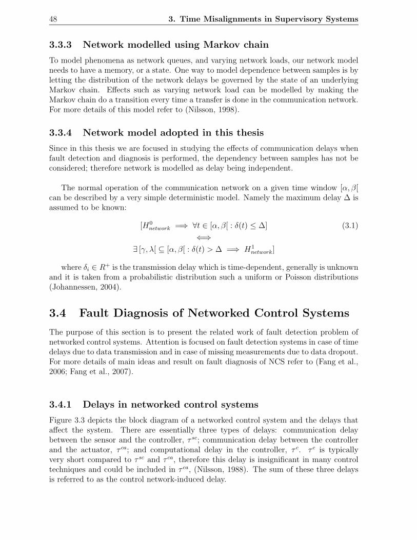
48 3. Time Misalignments in Supervisory Systems
3.3.3 Network modelled using Markov chain
To model phenomena as network queues, and varying network loads, our network modelneeds to have a memory, or a state. One way to model dependence between samples is byletting the distribution of the network delays be governed by the state of an underlyingMarkov chain. Effects such as varying network load can be modelled by making theMarkov chain do a transition every time a transfer is done in the communication network.For more details of this model refer to (Nilsson, 1998).
3.3.4 Network model adopted in this thesis
Since in this thesis we are focused in studying the effects of communication delays whenfault detection and diagnosis is performed, the dependency between samples has not beconsidered; therefore network is modelled as delay being independent.
The normal operation of the communication network on a given time window [α, β[can be described by a very simple deterministic model. Namely the maximum delay ∆ isassumed to be known:
[H0network =⇒ ∀t ∈ [α, β[ : δ(t) ≤ ∆] (3.1)
⇐⇒∃ [γ, λ[ ⊆ [α, β[ : δ(t) > ∆ =⇒ H1
network]
where δi ∈ R+ is the transmission delay which is time-dependent, generally is unknownand it is taken from a probabilistic distribution such a uniform or Poisson distributions(Johannessen, 2004).
3.4 Fault Diagnosis of Networked Control Systems
The purpose of this section is to present the related work of fault detection problem ofnetworked control systems. Attention is focused on fault detection systems in case of timedelays due to data transmission and in case of missing measurements due to data dropout.For more details of main ideas and result on fault diagnosis of NCS refer to (Fang et al.,2006; Fang et al., 2007).
3.4.1 Delays in networked control systems
Figure 3.3 depicts the block diagram of a networked control system and the delays thataffect the system. There are essentially three types of delays: communication delaybetween the sensor and the controller, τ sc; communication delay between the controllerand the actuator, τ ca; and computational delay in the controller, τ c. τ c is typicallyvery short compared to τ sc and τ ca, therefore this delay is insignificant in many controltechniques and could be included in τ ca, (Nilsson, 1988). The sum of these three delaysis referred to as the control network-induced delay.

3.4. Fault Diagnosis of Networked Control Systems 49
Controllernode
Actuatornode Process Sensor
node
u(t) y(t)
Network
Figure 3.3: Delays in NCS: communication delay between the sensor and the controller,τ sc; communication delay between the controller and the actuator, τ ca; and computationaldelay in the controller, τ c which could be included in τ ca, (Nilsson, 1988).
A Networked Control Systems can be modelled by:
x(t) = f(x(t), u(t− τ ca), ϕ(t)) (3.2)
y(t) = g(x(t), u(t− τ ca), ϕ(t)) (3.3)
y(t) , y(t− τ sc) (3.4)
where y(t) is the most updated output received by the controller.
It is evident that the networked-induced delay in NCS could influence the performanceof traditional fault detection systems. For example, in (Ye et al., 2004; Ye et al., 2006) itis shown that due to the influence of the network-induced delay, an observer based faultdetection system designed for a non-networked control system can’t fulfill the basic re-quirement on residual generation anymore when it is used for a NCS, i.e., with the delay,the residual signal of a traditional residual generator will not be able to be decoupledfrom the control input any longer. (Sauter and Boukhbza, 2006) also studied the effectof unknown networked induced delays on conventional observer based residual generator.It is shown that the detection performances may be reduced due to the sensitivity of theresiduals to the delays.
The effect of communication delay depend upon the communication topology. Indistributed control systems the FDI unit can be located in different forms:
• located at the same node of the controller (Shanbin et al., 2006; Zhang and Ding,2007). In this configuration the residual generator can directly obtain the controlinput u(t) from the controller and it must get access to the measurement y(t) throughthe network. Therefore residual will be affected just by the delay τ sc.
• the FDI unit can be implemented as an algorithm in one node of the network(Llanos et al., 2007), see Figure 3.4. In this structure the residual computation can

50 3. Time Misalignments in Supervisory Systems
Controllernode
Actuatornode Process Sensor
node
FDI node
u(t) y(t)
Network
Figure 3.4: Structure adopted in this thesis: the FDI unit of the NCS is placed in aremote node.
be affected by the communication delay between the sensor and the FDI node, δsfdi;and the communication delay between the controller and the FDI node, δcfdi.
• and even, if we are dealing with large interconnected systems, the residual compu-tation algorithm can be implemented following different architectures: centralized,decentralized or autonomous distributed, (Sauter et al., 2006).
This thesis is focused on the fault detection and diagnosis of NCS with not onlynetwork delays but also data dropout. In this thesis the FDI unit has been imple-mented as an algorithm in one node of the network, see Figure 3.4. Section3.5 presents in more details the problem formulation of communication delays in residualcomputation under above mentioned implementation.
3.4.2 Related works in Fault Diagnosis of Networked ControlSystems
In most of the related works the NCS were modelled as different simplified time-delaysystems. Based on these models, many existed results, such as state observer and filteringtheory, developed originally for time-delay systems could be utilized for fault diagnosis ofNCS. Despite we do not use time-delay systems models in this thesis, relatedworks are here presented.
Approaches based on state estimation and observer theory of time-delay sys-tems
In this approaches the NCS model given by equation (3.2 and (3.4) is modified in orderto take into account the delays in the state vector,x(t):

3.4. Fault Diagnosis of Networked Control Systems 51
x(t) = f(x(t− νi), u(t− τ ca), ϕ(t)) (3.5)
y(t) = g(x(t− νi), u(t− τ ca), ϕ(t)) (3.6)
y(t) , y(t− τ sc) (3.7)
where νi denotes time delays in the state.
The work by (Yang and Saif, 1998) is the first paper to deal with the fault detectionproblem for time delay systems. A reduced-order unknown input observer was proposedto detect and identify the actuator and sensor faults for a class of state-delayed dynamicsystems, in which the faults as well as other effects such as disturbances and higher-ordernonlinearities were considered as unknown inputs. With some assumptions on the struc-ture of system and distribution matrices, the completely unknown input decoupling fromthe residual is achieved.
In (Ding et al., 2002), a weighting transfer function matrix was first developed todescribe the desired behaviour of residual respect to fault, and the observer-based faultdetection filter for a class of linear systems with time-varying delays was designed insuch a way that the error between the generated residual and fault (or, more generallyweighted fault) is as small as possible in the sense of H∞ -norm. The designing of theobserver-based fault detection filter was then formulated into an H∞ - model matchingproblem and, with the aid of an optimization tool, such as the linear matrix inequalitytechnique, the problem has been solved.
The work in (Zhong et al., 2005) dealt with the fault detection problem for linear sys-tems with L2 -norm bounded unknown input and multiple constant time delays. Observer-based fault detection filter has been developed such that a robustness/sensitivity basedperformance index was minimized. The key idea of this study is the introduction of anew fault detection filter as residual generator and the extension of an optimization faultdetection method for linear time invariant systems in (Ding et al., 2000) to the time-delaysystems. A sufficient condition to the solvability of fault detection filter has been derivedin terms of Riccati equation and a solution has been obtained by suitably choosing of afilter gain matrix and post-filter.
In (Zhong et al., 2004), the above mentioned optimization fault detection approach of(Ding et al., 2000) has been further modified to a class of neutral time-delay systems.
With a structure restriction on fault distribution, the work by (Jiang et al., 2002a;Jiang et al., 2002b; Jiang et al., 2003) developed an adaptive observer to the fault iden-tification for both linear systems with multiple state time delays and a class of nonlinearsystems
More recently, a new adaptive observer was proposed for the robust fault detectionand identification of uncertain linear time-invariant systems with multiple constant time-delays in both states and outputs by (Jiang and Zhou, 2005).

52 3. Time Misalignments in Supervisory Systems
In (Zheng et al., 2003b) they regard NCS as a sampled-data control systems withtime-delays and set up its mathematical model. By constructing a memoryless reduced-order fault observer (Trinh and Aldeen, 1997), they achieve the fault detection of NCS.This observer-based fault detection approach for NCS is only serving as typical example.
With different assumptions and simplified systems models of NCS, variety existedworks related to state estimation and observer for time-delay system can be extended toor used for NCS, and then for fault diagnosis algorithms for NCS were developed, such asthe results presented in (Xie et al., 2005; Zheng et al., 2003a; Zheng et al., 2004; Zhenget al., 2005).
(Ding and Zhang, 2005) proposed an advanced observer-based scheme for the monitor-ing of distributed networked control systems. They do not attack directly the problem ofdelays but they consider that if the network load is minimised then the data transmissiondelays are reduced. Consequently, they design a two-level monitoring system. For eachsubsystem, a fault detection unit based on observer is embedded, which only makes use oflocal control input and measured output signals. In the global level, a central monitoringsystem is designed, which satisfies the required monitoring performance. Instead of col-lecting measured output signals from all subsystems, the inputs to the central monitoringsystem are the residual signals provided by the local fault detection units. In this way, aquantization can be used for transmission of signals. A reduced data transmission is thusachieved and the data transmission delays are expected to be smaller.
Approaches based on filtering
In this approaches the deterministic system model:
x(t) = f(x(t), u(t), ϕ(t)) (3.8)
y(t) = g(x(t), u(t), ϕ(t)) (3.9)
is modified. (Ye et al., 2006) show that the unknown network-induced delay introducesan unknown additive item h(t) into plant model:
x(t) = f(x(t), u(t), h(t), ϕ(t)) (3.10)
y(t) = g(x(t), u(t), ϕ(t)) (3.11)
Therefore, when the network-induced delay is random, the unknown item h(t) can alsobe regarded as a random disturbance. So a natural idea to reduce the influence of thisdisturbance is low-pass filtering the residual signal of a traditional generator. However,the idea could not be realized by only designing a traditional optimal residual genera-tor first and then adding a low-pass filter to its output, because the optimization of thetraditional residual generator does not mean that the new system consisting of it and apost-filter is still optimal. So they consider both parts of the new system (i.e. the residualgenerator and the low-pass filter) when designing the fault detection system.

3.5. Time Misalignments in Residual Computation 53
A robust fault isolation filter for networked control systems with network-induceddelays and multiple faults has been designed in (Shanbin et al., 2006). Where the com-munication delay between the sensor and the controller, τ sc
k and the communication delaybetween the controller and the actuator, τ ca
k are lumped together as a single delay, whichis assumed to be random and governed by a Markov chain. Then, the effect of network-induced delays introduced into the control loop is regarded as time-varying disturbance.Based on this model, a fault isolation filter for fault detection of such networked controlsystems is then parameterized in order to generate the residuals having directional prop-erties in response to a particular fault and decoupling from the disturbance.
Based on the study on the frequency domain characteristics of parity space approach(Ye et al., 2000; Zhang et al., 2006), a new fault detection approach based on parityspace and Stationary Wavelet Transform (SWT) was proposed (Ye et al., 2004), addingSWT filters to an ordinary parity space based residual generator and considering both,the residual generators and the filters, in optimal design.
Fault detection of networked control systems with missing measurements
Another problem, close to data delays, also introduced by the networks is the datadropout. (Zhang et al., 2004) studied the fault detection problem of networked con-trol systems with missing measurements due to data dropout. First, in order to cope withmissing measurement, the structure of standard model-based residual generator is modi-fied and dynamic network resource allocation is suggested. The dynamics of the residualgenerator is shown to be characterised by a discrete-time Markovian jump linear system.Then a residual evaluation scheme is developed aiming to reduce false alarm rate causedby missing measurement. Further, they proposed a co-design approach of time-variantresidual generator and threshold to improve the dynamics and the sensitivity of the faultdetection system to the faults. Related to this work is also the work on filtering in case ofmissing measurements. A detailed up-to-date summary of research in this direction couldbe found in (Wang et al., 2003).
3.5 Time Misalignments in Residual Computation
3.5.1 Problem formulation
Consider the deterministic system modelled by
x(t) = f(x(t), u(t), ϕ(t)) (3.12)
y(t) = g(x(t), u(t), ϕ(t)) (3.13)
where x(t) ∈ Rn, u(t) ∈ Rr, y(t) ∈ Rm and ϕ(t) ∈ Rq are respectively the state, input,output and fault vector, and f and g are given smooth vector fields.

54 3. Time Misalignments in Supervisory Systems
Residual computation node
Node 1
Smart sensor
z1
z3
z2
))(()( tzGtric
Node 2
Local controller
Figure 3.5: Data decomposition in distributed system
Data decomposition in distributed systems
In distributed control systems, the residual computation form is implemented as an algo-rithm in one node of the network. At each time t its input data are noted as
z(t) ,
(
u(t)y(t)
)
where y(t) (and also u(t)) is the vector obtained by expanding y(t) with its derivativesy(t), y(t), . . . up to some derivation order.
According to the overall system distributed architecture, z(t) is decomposed into a setof subvectors zi(t), i ∈ I and the computation form of the residual vector writes
r(t) = Gc (zi(t), i ∈ I) (3.14)
The subvectors zi(t) are such that all variables in zi(t) are transmitted in one singlepacket through the communication network. Note that this does not imply that all thevariables produced at a given node are transmitted in one single packet. As shown inFigure 3.5
z(t) = (zT1 (t), zT
2 (t), zT3 (t))T
where z1 is produced and transmitted by node 1 (a smart sensor), while z2 ∪ z3 areproduced by node 2 (a local controller). The data are decomposed into packet z2 andpacket z3 for their transmission through the communication system.
As result, the residual vector (3.14) designed under the assumption of perfect commu-nication might create false alarms due to transmission delays.

3.5. Time Misalignments in Residual Computation 55
The incidence of transmission delays
Due to the transmission delays the data zi(t) generated at the production nodes andthe data zi(t) available at the residual computation node must be distinguished. Oneobviously has
zi(t) = zi(t− δi), i ∈ I (3.15)
where δi ∈ R+ is the transmission delay i.e. the data zi was produced at time t− δi, andit was received only at time t. Transmission delays δi may be time-dependent and theygenerally are unknown. The normal operation of the communication network on a giventime window [α, β[ can be described by a very simple deterministic model. Namely themaximum delay ∆ is assumed to be known:
[H0network =⇒ ∀i ∈ I,∀t ∈ [α, β[ : δi ≤ ∆] (3.16)
⇐⇒[∃i ∈ I,∃ [γ, λ[ ⊆ [α, β[ : δi > ∆ =⇒ H1
network]
If communication delays are not taken into account residual computation can be per-formed as
r(t) = Gc(zi(t), i ∈ I) (3.17)
but using data which are taken from the system at different time instants would ob-viously result in false alarms.
Taking into account communication delays by using future values of the arguments,as in (3.18), is obviously impossible.
r(t) = Gc(zi(t+ δi), i ∈ I) (3.18)
A possible solution for decreasing the false alarms rate due to communication delaysis by increasing the decision threshold, at the cost of reducing the sensitivity to faults.
Equation (3.18) has been used for considering the effect of communication delays inresidual generation. If the analysis of the residual generator want also to be considered,equation (3.18) can be generated by any observer based residual generator which allowsto control the dynamic of the residual.
In this thesis, two techniques aiming at the minimization of the false alarms caused bytransmission delays without increasing the number of missed detection are proposed andexplained in Chapters 4 and 6, respectively. The first one relies on the explicit modellingof communication delays and their most likely estimation, and the second one proposesan optimal dynamic alignment of data in a time window (Dynamic Time Warping).

56 3. Time Misalignments in Supervisory Systems
3.6 Time Misalignments in Signal Based Fault Diag-
nosis
The time misalignments affect the non model based fault diagnosis particulary on thetechniques that use the comparison and matching of temporal signals for diagnosis pur-pose.
3.6.1 Problem formulation
In non model based fault diagnosis the deterministic model given by equations (3.12) and(3.13) can not be considered anymore because function f and g are unknown. The onlyinformation we have from the process are the input u(t) and the output y(t) signals rep-resented as time-series which are a rich source information that can be used for diagnosispurpose.
Pattern classification or signal comparison (Colomer, 1998; Webb, 2002) is a popularmethod for finding similar signals in historical data. The challenge in this approach re-sults from the fact that, because of the nature of the industrial processes, signals thatresult from the two instances of the same change are not exact replicates. In others words,there are deviations between the the two instances. The differences could be in the length(total time) of the two signals or in the magnitudes or profiles of the variables. Therefore,direct comparison of two signals would be incorrect, because there is no guarantee thatthe corresponding segments of the signal are being compared.
Most of algorithm that operate with time-series of data use the Euclidean distanceor some variation. However, Euclidean distance could produce an incorrect measure ofsimilarity because it is very sensitive to distortions in the time axis (time misalignments),Figure (3.6) gives an example of time misalignments effects when comparing two time-series. Therefore, robust yet sensitive methods for comparing unsynchrinised signals arean active area of research.
3.6.2 Previous work in signal comparison for fault diagnosis
Due to significant advances in data collection and storage, vast amount of historical datais becoming commonly available. This data is a rich source of information about theprocess that can be used to improve plant operation. Multivariate statistics such as prin-cipal components analysis (PCA) have been widely used for process data classificationand fault detection and diagnosis (Kano et al., 2001; Chen and Liao, 2002; Chiang andBraatz, 2003). PCA reduces the dimensionality of data with minimum loss of informa-tion by projecting high dimensional data onto uncorrelated vectors. The projections arechosen so that the maximum amount of information, measured in terms of its variability,is retained in the smallest number of dimensions.
(Krzanowski, 1979) defined the PCA similarity factor for measuring the similarity of

3.6. Time Misalignments in Signal Based Fault Diagnosis 57
0 10 20 30 40 50 60 70 80 90 100(b)
0 10 20 30 40 50 60 70 80 90 100(a)
Figure 3.6: Two unsynchronised signals. a) erroneous comparison due to time misalign-ment; b) intuitive alignment feature
different groups of data. The PCA similarity factor compares the reduced subspaces:
SPCA =1
k
k∑
p=1
k∑
q=1
cos2 θpq (3.19)
where θpq is the angle between the pth principal component of dataset S and theqth principal component of dataset T . (Raich and Cinar, 1997) used the PCA similarityfactor for diagnosis process fault. (Singhal and Seborg, 2002) modified the PCA similarityfactor by weighing the principal components with the square root of their correspondingeigenvalue, λ.
SλPCA =
∑kp=1
∑kq=1 λ
Spλ
Tq cos2 θpq
∑kp=1 λ
Spλ
Tp
(3.20)
A major limitation of the classical PCA-based approaches is that the PCA similarityfactor is only applicable for stationary signals. To extend them to nonstationary signals,(Srinivasan et al., 2004) proposed a dynamic PCA-based similarity factor (Sλ
DPCA) thataccounts for the temporal evolution of the signal. The main advantage of the PCA-basedmethods is their inherent ability to deal with multivariate signals and their low compu-tational requirements. One strong assumption of PCA-based methods is that all batcheshave equal duration and all are synchronized.
Another family of data-driven approaches use signal comparison in order to overcomethis. These approaches are based on the precept that the same types of faults show similarfeatures in the process signal. This assumption is satisfied by most common normal and

58 3. Time Misalignments in Supervisory Systems
faulty operating states in processes. By comparing the online signal with a database ofsignals corresponding to the different fault classes, any fault in the process can be diag-nosed. The challenge in these methods is that it is normal for two similar signals to beslightly different or misaligned and not match each other perfectly. This synchronizationproblem can be overcome using Dynamic Time Warping (DTW). In this thesis we pro-posed a slight modification of DTW in order to adapt it for on-line application. Chapters6 and 7 are devoted to explain the main particularities of the new algorithm, as well asits application on a knowledge-based method for fault diagnosis, known as Case basedReasoning.

3.7. Conclusions 59
3.7 Conclusions
Control over data networks has many advantages compared with traditional control sys-tems, such lower cost, greatly reduced wiring, weight and power, simpler installation andmaintenance and higher reliability. However, the data dropout, limited bandwidth, timedelay due to data transmission, asynchronous clock among network nodes and other pe-culiarities of networks could degrade the performances of the closed-loop systems andeven destabilize them. Above problems have been intensively studied by the controlcommunity in the last several years including: analysis of impact of network on controlperformance, design of control algorithm taking into account the above factors and pro-posal of new network protocol suitable for control. However only a few studies of theimpact of the communication network on the diagnosis of continuous systems have beenpublished. Namely, in model-based Fault Detection and Isolation (FDI) a set of residualsis computed, that should be ideally zero in the fault-free case and different from zero, inthe faulty case. However, in practice, residuals are different from zero, not only becauseof measurement noise, unknown inputs, and modelling uncertainties but also because oftransmission delays introduced by the communication networks.
Most of the related works attack the fault detection problem of NCS with randomtime delay in two ways: extending or directly using the existed state estimation and ob-server theory of time-delay system to develop dedicated fault detection method for NCS,and developing fault diagnosis methods which are robust to an unknown item producedby the network-induced random time-delay. In both cases a modification of the systemmodel in order to take into account the communication delays is introduced. This thesisproposes a solution for tame-delays effect in NCS when performing FDI. The solutiondoesn’t modify the system model and is based on the explicit modelling of communica-tion delays and on their best-case estimation. The technique is explained in next Chapter.
Concerning the FDI with data dropout, this thesis proposes a technique for falsealarms reduction due to data dropout, the solution is based on the residual behaviourand the communication status. The technique is explained in Chapter 5.
Regarding the signal-based fault diagnosis, there are several techniques for comparingtime-series for fault diagnosis purpose, however most of them do not explicitly considerthe problem of time-misalignments. A method known as dynamic time warping (DTW)allows a nonlinear alignment within two signals. A shortcoming of this method is itsexpensive computational cost (in both time and memory) which make it normally usefulonly for off-line applications. This has motivated a slight modification of DTW in orderto adapt it for on-line application. Chapters 6 and 7 are devoted to explain details aboutDTW, the main particularities of the new algorithm, as well as its application on Casebased Reasoning.

60 3. Time Misalignments in Supervisory Systems

Chapter 4
Delay Estimation for ResidualComputation
4.1 Introduction
As has been seen en previous chapter residuals that should theoretically be zero in the nonfaulty case might create false alarms as the result of transmission delays. The false alarmsrate can be decreased by increasing the decision threshold, at the cost of reducing thesensitivity to faults. In this chapter, a technique aiming at the minimization of the falsealarms caused by transmission delays without increasing the number of missed detectionis proposed. It relies on the explicit modelling of communication delays, and their mostlikely estimation (Llanos et al., 2006; Llanos et al., 2007).
The chapter is organized as follows: Section 4.2 presents the influence of transmissiondelays. The decision procedure under unknown transmission delays is analysed in Section4.3. An optimization technique for the estimation of unknown delays is described inSection 4.4. Illustrative examples are shown in Section 4.4.1 and 4.5. Finally someconcluding remarks are given in Section 4.6.
4.2 Influence of communications delays in residual
computation
As was stated in section 3.5.1, in distributed control systems, the residual computationform is implemented as an algorithm in one node of the network.
If communication delays are not taken into account residual computation can be per-formed as
r(t) = Gc(zi(t), i ∈ I) (4.1)
where zi(t) is the data available at the residual computation node. Using data whichare taken from the system at different time instants would obviously result in false alarms.
61
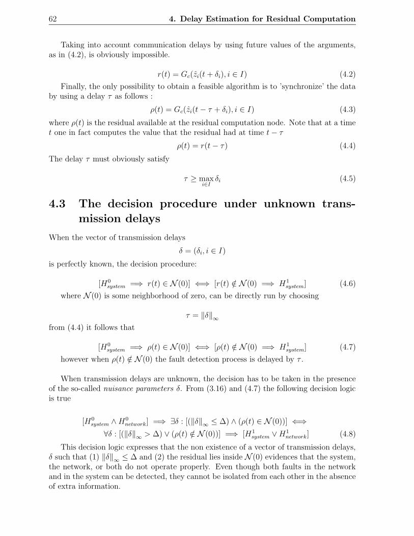
62 4. Delay Estimation for Residual Computation
Taking into account communication delays by using future values of the arguments,as in (4.2), is obviously impossible.
r(t) = Gc(zi(t+ δi), i ∈ I) (4.2)
Finally, the only possibility to obtain a feasible algorithm is to ’synchronize’ the databy using a delay τ as follows :
ρ(t) = Gc(zi(t− τ + δi), i ∈ I) (4.3)
where ρ(t) is the residual available at the residual computation node. Note that at a timet one in fact computes the value that the residual had at time t− τ
ρ(t) = r(t− τ) (4.4)
The delay τ must obviously satisfy
τ ≥ maxi∈I
δi (4.5)
4.3 The decision procedure under unknown trans-
mission delays
When the vector of transmission delays
δ = (δi, i ∈ I)is perfectly known, the decision procedure:
[H0system =⇒ r(t) ∈ N (0)] ⇐⇒ [r(t) /∈ N (0) =⇒ H1
system] (4.6)
where N (0) is some neighborhood of zero, can be directly run by choosing
τ = ‖δ‖∞from (4.4) it follows that
[H0system =⇒ ρ(t) ∈ N (0)] ⇐⇒ [ρ(t) /∈ N (0) =⇒ H1
system] (4.7)
however when ρ(t) /∈ N (0) the fault detection process is delayed by τ .
When transmission delays are unknown, the decision has to be taken in the presenceof the so-called nuisance parameters δ. From (3.16) and (4.7) the following decision logicis true
[H0system ∧H0
network] =⇒ ∃δ : [(‖δ‖∞ ≤ ∆) ∧ (ρ(t) ∈ N (0))] ⇐⇒∀δ : [(‖δ‖∞ > ∆) ∨ (ρ(t) /∈ N (0))] =⇒ [H1
system ∨H1network] (4.8)
This decision logic expresses that the non existence of a vector of transmission delays,δ such that (1) ‖δ‖∞ ≤ ∆ and (2) the residual lies inside N (0) evidences that the system,the network, or both do not operate properly. Even though both faults in the networkand in the system can be detected, they cannot be isolated from each other in the absenceof extra information.

4.4. Estimating the transmission delays 63
4.4 Estimating the transmission delays
Let the system fault detection neighborhood N (0) be defined by
N (0) = {ρ : J (ρ) ≤ σ}where ∀ρ 6= 0, J (ρ) > 0, J (0) = 0, for example J (ρ) = ρTQρ with Q > 0 and σ > 0
is a given decision threshold. Checking the property H0system ∧ H0
network can be done bysolving the following optimization problem
δ = arg min‖δ‖∞≤∆
J(ρ(t)) (4.9)
where ρ(t) = Gc(z(t−τ+δ)). Let τ =∥
∥
∥δ∥
∥
∥
∞, ρ(t) = Gc(z(t−τ+δ)) and J(t) = J(ρ(t)),
then the following interpretation holds :
(1) δ is the ”most likely” vector of admissible delays in the sense that the functionJ(t) associated with the delayed residual ρ(t) is minimum
(2) This residual may or may not be compatible with the hypothesis that the systemoperates in a nominal way, and therefore the decision logic (4.8) becomes:
J(t) > σ =⇒ H1system
Finally it should be noted that the estimation of δ by (4.9) implements a sufficientcondition-based decision logic. Indeed, if the minimal value J(t) associated with δ doesnot satisfy J(t) ≤ σ then no other estimation will do. However, the set{δ : [‖δ(t)‖∞ ≤ ∆] ∧ [ρ(t) ∈ N (0)]} may contain more than one element.
4.4.1 Searching for a minimum
The cost function J(ρ(t)) = J [Gc(z(t− τ + δ))] is in general a nonlinear function of theadjustable parameters δ, and its minimum can be found using well known iterative searchmethods (Reklaitis et al., 1983). However, since the problem is to be solved in real time,it is of interest to study the conditions under which the estimation δ can be found quicklyand accurately. Note that even when a dynamic feedback control loop is involved, the on-line search for a minimum, being a part of the Fault Detection and Isolation algorithm, canbe run at a much lower frequency than the one associated with the control computation,for systems where faults are not critical (should faults be critical, it can be assumed thatthe network would have been designed so as to make transmission delays negligible).
Persistent excitation condition
Assuming that all functions involved are differentiable, the solution of the optimizationproblem (4.9) satisfies the necessary condition :
∂J(ρ(t))
∂δi+ µi = 0, i ∈ I (4.10)
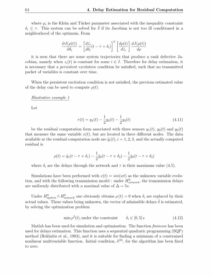
64 4. Delay Estimation for Residual Computation
where µi is the Khun and Tucker parameter associated with the inequality constraintδi ≤ τ . This system can be solved for δ if its Jacobian is not too ill conditioned in aneighborhood of the optimum. From
∂J(ρ(t))
∂δi=
[
dzi
dδi(t− τ + δi)
]T [
dρ(t)
dzi
]
dJ(ρ(t))
dρ
it is seen that there are some system trajectories that produce a rank defective Ja-cobian, namely when zi(t) is constant for some i ∈ I. Therefore for delay estimation, itis necessary that a persistent excitation condition be satisfied, such that no transmittedpacket of variables is constant over time.
When the persistent excitation condition is not satisfied, the previous estimated valueof the delay can be used to compute ρ(t).
Illustrative example 1
Let
r(t) = y1(t)−1
2y2(t)−
1
2y3(t) (4.11)
be the residual computation form associated with three sensors y1(t), y2(t) and y3(t)that measure the same variable x(t), but are located in three different nodes. The dataavailable at the residual computation node are yi(t), i = 1, 2, 3, and the actually computedresidual is
ρ(t) = y1(t− τ + δ1)−1
2y2(t− τ + δ2)−
1
2y3(t− τ + δ3)
where δi are the delays through the network and τ is their maximum value (4.5).
Simulations have been performed with x(t) = sin(wt) as the unknown variable evolu-tion, and with the following transmission model : under H0
network, the transmission delaysare uniformly distributed with a maximal value of ∆ = 5s.
Under H0system ∧H0
network one obviously obtains ρ (t) = 0 when δi are replaced by their
actual values. These values being unknown, the vector of admissible delays δ is estimated,by solving the optimization problem
min ρ2(t), under the constraint δi ∈ [0, 5] s (4.12)
Matlab has been used for simulation and optimisation. The function fmincon has beenused for delays estimation. This function uses a sequential quadratic programming (SQP)method (Reklaitis et al., 1983), and it is suitable for finding a minimum of a constrainednonlinear multivariable function. Initial condition, δ(0), for the algorithm has been fixedto zero.

4.4. Estimating the transmission delays 65
In order to study the benefits of delay estimation to optimize residual computation,neither unknown inputs (noise or disturbances) nor uncertainties have been considered.The analysis has been focused on the performance of the method to reduce false alarmsin the absence of faults. Figure 4.1 depicts the residual computed without and with thedelay estimation in a fault free situation (r(t) above and ρ(t) below). The value of w was0.05rad.s−1. It is well known that false alarms can always be avoided (e.g. by never firingany alarm). This can be seen on the figure, which shows that false alarms are avoided inboth cases, but at the cost of one order of magnitude on the decision threshold ( ±0.19instead of ±0.02), which means worse performances when faults will be present (largermissed detection rate, bigger size for faults to be detectable).
It is worth noting that, at particular (periodical) times the residual ρ(t) has significantdeviations with respect to zero. Those times correspond with the maximal and minimalvalues of the sinusoidal signal x(t). Indeed, in those cases the small variability of thesignals does no guarantee the fulfillment of the persistent excitation condition. Never-theless, even in that situation the residual ρ(t) is one order of magnitude smaller than r(t).
The error distributions between actual and estimated delays are depicted in the threehistograms of Figure 4.1. The errors are close to zero, which means a good estimation.For the first delay δ1, there are less negative errors than for the other delays, this is dueto the fact that δ1 is associated with the largest term in the residual. Consequently, theuse of gradient methods in the optimization procedure forces a faster adjustment. It isimportant to remark that the uncertainty reflected in the comparison does not affect thecomputation of the residual ρ(t) and it is just relevant when the persistent excitationcondition is not fulfilled.
Local minima
The search for a minimum is started out from an initial guess on the parameters δ(0)
and in general it will converge towards a local minimum. Starting with zero at the verybeginning and taking the last estimate of the transmissions delays as the initial guess forthe next estimation seems to be a good approach when the exploitation conditions of thenetwork do not change at a faster rate than the rate at which residuals are computed.Converging towards a local minimum is a source of false alarms, since the estimation δ maylead to ρ(t) /∈ N (0) while the global minimum, say δ∗, would have provided ρ∗(t) ∈ N (0).In special cases, such as linear systems and convex cost functions, global minima willbe found, but in more general cases, algorithms which avoid getting trapped in a localminimum are to be used (Goldberg, 1989).
False alarm vs missed detection
Given certain threshold values, statistical hypothesis theory can be applied to predict thefalse alarm and missed detection rates based on the statistics of the data. Increasing thethreshold (shifting the vertical line to the right in Figure 4.2a) decreases the false alarmrate but increases de missed detection rate. Attempts to lower the false alarm rate areusually accompanied with an increase in the missed detection rate, with the only ways

66 4. Delay Estimation for Residual Computation
0 100 200 300 400 500 600−0.5
−0.190
0.19
0.5
r(t)
0 100 200 300 400 500 600−0.05
−0.020
0.02
0.05
ρ(t)
0 100 200 300 400 500 6000
2
4
δ 1act−
δ 1est
0 200 4000
2
4
0 100 200 300 400 500 600−2
0
2
4
δ 2act−
δ 2est
0 100 200 300−2
0
2
4
0 100 200 300 400 500 600−2
0
2
4
δ 3act−
δ 3est
0 100 200 300−2
0
2
4
Figure 4.1: Residual in fault free situation and comparison of actual and estimated delays
to get around this tradeoff being to collect more data, or to reduce the normal processvariability (e.g., through installation of sensors of higher precision). The value of the typeI error (false alarms), also called the level of significance λ, specifies the degree of tradeoffbetween the false alarm rate (Type I error) and the missed detection rate (Type II error)when deciding the presence of faults in the system.
The proposed optimisation technique aims to minimise the false alarm rate caused bytransmission delays without increasing the missed detection rate. Figure 4.2b) shows theintuitive idea.
Illustrative example 2
Continuing with example 1, table 4.1 gathers the decision thresholds that must be se-lected in order to avoid false alarms, for increasing values of w. It is seen that the larger w,the larger the threshold. Fixing the bandwidth of the communication channel and increas-ing the frequency of the signal to be transmitted decreases the quality of the transmission.It can be noted that by choosing larger thresholds to avoid false alarms, one can expectthe missed detection rate during faulty situations to be deteriorated, as can be seen below.
Table 4.2 and table 4.3 present the missed detection rate associated with differentadditive faults (bias values of 0.05, 0.1, 0.15 and 0.2) on residuals r(t) and ρ(t) of example1. And different signal dynamics (w values of 0.05, 0.11, 0.15, 0.21 and 0.31rad.s−1). Notethat in spite of the improvement associated with the estimation of the transmission delays,

4.4. Estimating the transmission delays 67
FalseAlarms
Misseddetections
FaultOK
FalseAlarms
Misseddetections
FaultOK
b)
a)Threshold
Figure 4.2: a)Level of significance, missed detections ( Type II error) and false alarms(Type I error). b)False minimisation without increasing the missed detections.

68 4. Delay Estimation for Residual Computation
missed detections are still possible when using residual ρ (t), but they are much less thanthe missed detections associated with residual r(t). In other words, the minimum size ofdetectable faults can be reduced using the residual ρ(t) instead of residual r(t) withoutincreasing the false alarms rate.
4.5 Application to a control position of a DC motor.
Figure A.1 depicts the schematic diagram of a control position for a DC motor. Theaim of this system is to control the position c(t) of the mechanical load according to thereference position u(t). This system has been taken from (Ogata, 1997).
The transfer function in open loop is:
C(s)
Ev(s)=
Km
s(Tms+ 1)(4.13)
where, C(s) = L[c(t)] and Ev(s) = L[ev(t)], ev(t) is the error between the output andthe input positions. Km and Tm are known parameters of the system.
Let
r(t) = Tmd2c(t)
dt2+dc(t)
dt−Kmev(t) (4.14)
be the residual computation form associated with the system, where c(t) and ev(t) areassumed to be produced in two different nodes of a distributed system, see Figure 4.4.The design of this residual is explained in more details in Appendix A.
The data available at the residual computation node are ev(t) and c(t), and the actuallycomputed residual is
ρ(t) = Tmd2c(t− τ + δ1)
dt2+dc(t− τ + δ1)
dt−Kmev(t− τ + δ2) (4.15)
where δi are the delays through the network and τ is their maximum value (4.5).
Simulations have been performed with Km = 5.5s−1 and Tm = 0.13s. u(t) has beenmodelled as an unit step signal and c(t) as its response.
In order to study the benefits of delay estimation to optimize residual computation,neither unknown inputs (noise or disturbances) nor uncertainties have been considered.
Table 4.1: Decision thresholds for r(t) and ρ(t).
w1 w2 w3 w4 w5 w6
0.05rad/s 0.11rad/s 0.15rad/s 0.21rad/s 0.26rad/s 0.31rad/sr(t) ±0.02 ±0.04 ±0.06 ±0.08 ±0.1 ±0.13ρ(t) ±5 × 10⁻⁴ ±0.001 ±0.002 ±0.003 ±0.004 ±0.005

4.5. Application to a control position of a DC motor. 69
Table 4.2: Missed detection rate for r(t).
bias w1 w2 w3 w4 w5 w6
value 0.05rad/s 0.11rad/s 0.15rad/s 0.21rad/s 0.26rad/s 0.31rad/s0.05 17% 98% 93% 100% 100% 100%0.1 0% 26% 66% 96% 96% 100%0.15 0% 3% 17% 68% 80% 910.2 0% 0% 2% 23% 56% 86%
Table 4.3: Missed detection rate for ρ(t).
bias w1 w2 w3 w4 w5 w6
value 0.05rad/s 0.11rad/s 0.15rad/s 0.21rad/s 0.26rad/s 0.31rad/s0.05 0% 0% 0% 3% 0% 10%0.1 0% 0% 0% 0% 4% 0%0.15 0% 0% 0% 0% 0% 0%0.2 0% 0% 0% 0% 0% 0%
The analysis has been focused on the performance of the method to reduce false alarmsin the absence of system faults and to reduce the missed detection rates in presence of asensor fault.
4.5.1 Considering delays in one signal
Let’s consider that delays are introduced only for the signal c(t), with the transmissionmodel H0
network ⇐⇒ δ1, where δ1 is uniformly distributed in the interval [0, 0.1] s.
Under H0system ∧ H0
network one obviously obtains ρ (t) = 0 when δ1 is replaced by its
actual value. When this value is unknown, the admissible delay δ is estimated, by solvingthe optimization problem
min ρ2(t), under the constraint δ1 ∈ [0, 0.1] s (4.16)
Matlab has been used for simulation and optimisation. The function fminbnd hasbeen used for delays estimation. The algorithm is based on the golden section searchand parabolic interpolation (Reklaitis et al., 1983). This function finds the minimum of
u
Figure 4.3: Schematic diagram of a control position for a DC motor.

70 4. Delay Estimation for Residual Computation
)1( +m
m
sTsK
+ -
U(s) C(s)Ev(s)
Residual computation node
Communication network
Figure 4.4: Block diagram of the system.
0 0.2 0.4 0.6 0.8 1 1.2 1.4 1.6 1.8 2
−10
0
10
r(t)
0 0.2 0.4 0.6 0.8 1 1.2 1.4 1.6 1.8 2
−2
−1
0
1
2
x 10−3
ρ(t)
0 0.2 0.4 0.6 0.8 1 1.2 1.4 1.6 1.8 20
0.02
0.04
0.06
0.08
0.1
time, s
δ(t)
erro
r
0 100 2000
0.02
0.04
0.06
0.08
0.1
Figure 4.5: Residual in fault free situation and comparison of actual and estimated delays
a function within a fixed interval, the interval fixed for simulation was [0, 0.1].
Fault free situation
Figure 4.5 depicts the residual computed without and with the delay estimation in a faultfree situation (r(t) above and ρ(t) below). Notice that during the transient response,defined by the interval [0, 1.03]s, the residuals are more sensitive to the actual delays thanduring the steady-state time window. It is well known that false alarms can always beavoided (e.g. by never firing any alarm). This can be seen on Figure 4.5, which showsthat false alarms are avoided in both cases, but at the cost of four orders of magnitude onthe decision threshold (±10 instead of ±1.5x10⁻³). This means worse performances whenfaults will be present (larger missed detection rate, bigger size for faults to be detectable).
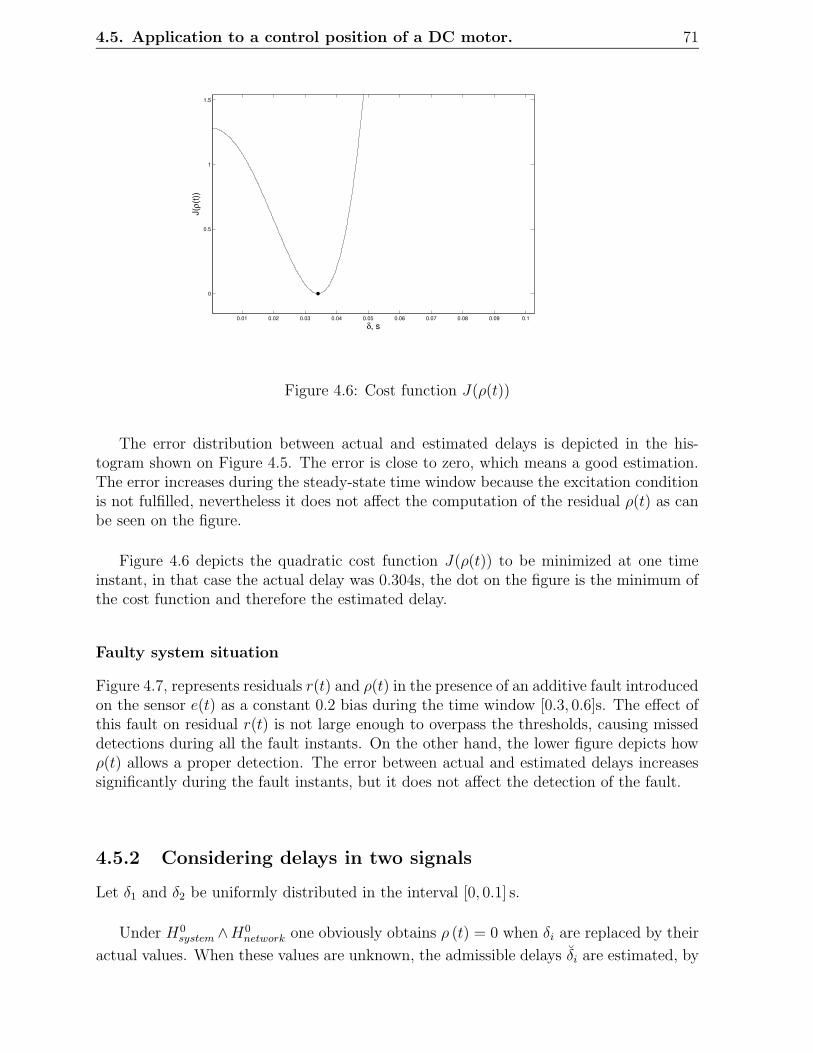
4.5. Application to a control position of a DC motor. 71
0.01 0.02 0.03 0.04 0.05 0.06 0.07 0.08 0.09 0.1
0
0.5
1
1.5
J(ρ(
t))
δ, s
Figure 4.6: Cost function J(ρ(t))
The error distribution between actual and estimated delays is depicted in the his-togram shown on Figure 4.5. The error is close to zero, which means a good estimation.The error increases during the steady-state time window because the excitation conditionis not fulfilled, nevertheless it does not affect the computation of the residual ρ(t) as canbe seen on the figure.
Figure 4.6 depicts the quadratic cost function J(ρ(t)) to be minimized at one timeinstant, in that case the actual delay was 0.304s, the dot on the figure is the minimum ofthe cost function and therefore the estimated delay.
Faulty system situation
Figure 4.7, represents residuals r(t) and ρ(t) in the presence of an additive fault introducedon the sensor e(t) as a constant 0.2 bias during the time window [0.3, 0.6]s. The effect ofthis fault on residual r(t) is not large enough to overpass the thresholds, causing misseddetections during all the fault instants. On the other hand, the lower figure depicts howρ(t) allows a proper detection. The error between actual and estimated delays increasessignificantly during the fault instants, but it does not affect the detection of the fault.
4.5.2 Considering delays in two signals
Let δ1 and δ2 be uniformly distributed in the interval [0, 0.1] s.
Under H0system ∧H0
network one obviously obtains ρ (t) = 0 when δi are replaced by their
actual values. When these values are unknown, the admissible delays δi are estimated, by
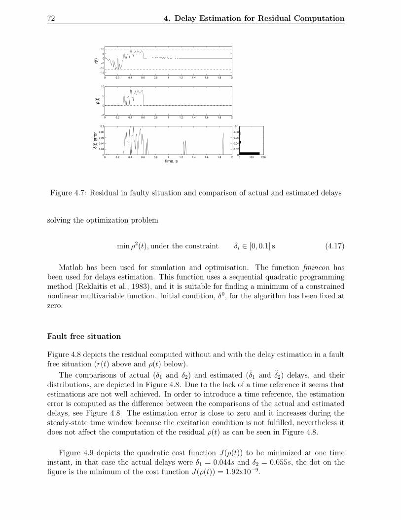
72 4. Delay Estimation for Residual Computation
0 0.2 0.4 0.6 0.8 1 1.2 1.4 1.6 1.8 2
−15
−10
−5
0
5
10
r(t)
0 0.2 0.4 0.6 0.8 1 1.2 1.4 1.6 1.8 2−5
0
5
10
ρ(t)
0 0.2 0.4 0.6 0.8 1 1.2 1.4 1.6 1.8 20
0.02
0.04
0.06
0.08
0.1
time, s
δ(t)
erro
r
0 100 2000
0.02
0.04
0.06
0.08
0.1
Figure 4.7: Residual in faulty situation and comparison of actual and estimated delays
solving the optimization problem
min ρ2(t), under the constraint δi ∈ [0, 0.1] s (4.17)
Matlab has been used for simulation and optimisation. The function fmincon hasbeen used for delays estimation. This function uses a sequential quadratic programmingmethod (Reklaitis et al., 1983), and it is suitable for finding a minimum of a constrainednonlinear multivariable function. Initial condition, δ0, for the algorithm has been fixed atzero.
Fault free situation
Figure 4.8 depicts the residual computed without and with the delay estimation in a faultfree situation (r(t) above and ρ(t) below).
The comparisons of actual (δ1 and δ2) and estimated (δ1 and δ2) delays, and theirdistributions, are depicted in Figure 4.8. Due to the lack of a time reference it seems thatestimations are not well achieved. In order to introduce a time reference, the estimationerror is computed as the difference between the comparisons of the actual and estimateddelays, see Figure 4.8. The estimation error is close to zero and it increases during thesteady-state time window because the excitation condition is not fulfilled, nevertheless itdoes not affect the computation of the residual ρ(t) as can be seen in Figure 4.8.
Figure 4.9 depicts the quadratic cost function J(ρ(t)) to be minimized at one timeinstant, in that case the actual delays were δ1 = 0.044s and δ2 = 0.055s, the dot on thefigure is the minimum of the cost function J(ρ(t)) = 1.92x10⁻⁹.

4.5. Application to a control position of a DC motor. 73
0 0.2 0.4 0.6 0.8 1 1.2 1.4 1.6 1.8 2
−10
0
10
r(t
)
0 0.2 0.4 0.6 0.8 1 1.2 1.4 1.6 1.8 2−0.5
0
0.5
ρ(t
)
0 0.2 0.4 0.6 0.8 1 1.2 1.4 1.6 1.8 2−0.1
0
0.1
time, s
δ 1−δ 1
0 50−0.1
0
0.1
0 0.2 0.4 0.6 0.8 1 1.2 1.4 1.6 1.8 2−0.1
0
0.1
time, s
δ 2−δ 2
0 20 40−0.1
0
0.1
0 0.2 0.4 0.6 0.8 1 1.2 1.4 1.6 1.8 2−0.1
0
0.1
time, sEst
imat
ion
erro
r
0 100 200−0.1
0
0.1
Figure 4.8: Residual in fault free situation, comparisons of the actual and estimated delaysand the estimation error.
0
0.02
0.04
0.06
0.08
0.1
00.01
0.020.03
0.040.05
0.060.07
0.080.09
0.10
1
2
3
4
5
6
7
8
9
δ1, s
X: 0.044Y: 0.055Z: 1.92e−009
δ2, s
J(ρ(
t))
Figure 4.9: Cost function J(ρ(t))

74 4. Delay Estimation for Residual Computation
0 0.2 0.4 0.6 0.8 1 1.2 1.4 1.6 1.8 2−20
0
20
r(t
)
0 0.2 0.4 0.6 0.8 1 1.2 1.4 1.6 1.8 2−10
0
10
ρ(t
)
0 0.2 0.4 0.6 0.8 1 1.2 1.4 1.6 1.8 2−0.1
0
0.1
time, s
δ 1−δ 1
0 50−0.1
0
0.1
0 0.2 0.4 0.6 0.8 1 1.2 1.4 1.6 1.8 2−0.1
0
0.1
time, s
δ 2−δ 2
0 20 40−0.1
0
0.1
0 0.2 0.4 0.6 0.8 1 1.2 1.4 1.6 1.8 2−0.2
0
0.2
time, sEst
imat
ion
erro
r
0 100 200−0.2
0
0.2
Figure 4.10: Residual in faulty situation, comparisons of the actual and estimated delaysand the estimation error.
Faulty system situation
Figure 4.10, represents residuals r(t) and ρ(t) in the presence of an additive fault intro-duced on the sensor e(t) as a constant 0.2 bias during the time window [0.3, 0.6]s. Theeffect of this fault on residual r(t) is not large enough to overpass the thresholds, causingmissed detections during almost all the fault instants. On the other hand, the lower figuredepicts how ρ(t) allows a proper detection. The estimation error increases significantlyduring the fault instants, but it does not affect the detection of the fault.
4.6. Conclusions 75
4.6 Conclusions
In model-based Fault Detection and Isolation a set of residuals is computed, that shouldbe ideally zero in the fault-free case and different from zero, in the faulty case. However,in practice, residuals are different from zero, not only because of faults but because ofmeasurement noise, unknown inputs modelling uncertainties and transmission delays indistributed systems. Using these residuals will produce false alarms and missed detections.
In this chapter it is shown that when transmission delays are known, it is possibleto take them into account in the residual computation, thus introducing a delayed butotherwise unchanged decision and avoiding false alarms due to delays. However, whendelays are unknown it is necessary to estimate them in order to compensate for their effectin the decision procedure. In this case, based on a very rough model of the delays, thechapter proposes to address the problem as an optimization problem. A search algorithmis used for the delay estimation by minimizing the residual under the constraints given bythe transmission model. When the persistent excitation condition is fulfilled, the delaysestimation can be carried out giving reliable results and avoiding false alarms.
The efficiency of the proposed approach is applied on a control position for a DCmotor.

76 4. Delay Estimation for Residual Computation

Chapter 5
Reduction of False Alarms in FaultDetection of Networked ControlSystems with Data Dropout
5.1 Introduction
In NCS the availability of data is affected by different casuistics depending on networkoperation (traffic, polling strategies, hubs and switches delays, etc.) resulting in datadropout at a specific node where they are analysed. Thus, the residual computation maybe inconsistent with the system state at the computation instant. Therefore, residualsthat should theoretically be zero during the normal operation conditions could generatefalse alarms as the result of missing data or dropouts. This effect can be observed asan increase of false alarm ratios. A common solution in such situations is to increasethe decision threshold according to the variability of the residual observed during datadropout. The cost of this action is a reduction of the sensitivity to faults and consequentlyan increase of missed detections.
In this Chapter, a formulation of how residual must be computed with available datais proposed. The aim is to reduce the false alarm ratio caused by data dropout withoutincreasing the number of missed detections.
The chapter is organized as follows: Section 5.2 presents the influence of data dropoutin residual computation. A technique for false alarms reduction due to data dropout isdescribed in Section 5.3. An illustrative example in a laboratory plant is shown in Section5.4. Finally some concluding remarks are given in Section 5.5.
77

785. Reduction of False Alarms in Fault Detection of Networked Control
Systems with Data Dropout
5.2 The influence of data dropout in residual compu-
tation
Consider the discrete time deterministic system modelled by
x(k + 1) = f(x(k), u(k), ϕ(k)) (5.1)
y(k) = g(x(k), u(k), ϕ(k)) (5.2)
where x(k) ∈ Rn, u(k) ∈ Rr, y(k) ∈ Rm and ϕ(k) ∈ Rq are respectively the state,control, output and fault vector, and f and g are given smooth vector fields.
Due to delays and possible dropout zi(k), generated at the production nodes, and zi(k)data available at the residual computation node are distinguished and their dependencewith the network communication status represented by:
zi(k) =
{
zi(k) if ψi(k) = 0zi(k − 1) if ψi(k) = 1
(5.3)
where ψi(k) is a stochastic variable which represents the data communication status.ψi(k) = 0 means that data at time k arrives correctly and therefore we are dealing withupdated values zi(k), while ψi(k) = 1 means that data has not properly arrived andtherefore the computation node only can use previous existent data zi(k − 1).
In general ψi(k) should be modeled by means of probability distribution Pi. Hence,the normal operation of the communication network on a given time window [α, β[ canbe described as a discrete deterministic model:
[H0network =⇒ ∀i ∈ I,∀k ∈ [α, β[ : ψi(k) ∼ Pi] (5.4)
⇐⇒[∃i ∈ I,∃ [γ, λ[ ⊆ [α, β[ : ψi(k) � Pi =⇒ H1
network]
where H0network represents the normal operation of the network in terms of Pi and
H1network is the hypothesis for anomalous behaviour.
5.3 Feasible residual computation
Residual computation computed as:
r(k) = Gc (zi(k), i ∈ I) (5.5)
can only be computed in case of availability zi(k)∀i ∈ I. Instead of this, only a residualr(k) can be computed with available data zi(k), at instant k:
r(k) = Gc (zi(k), i ∈ I) (5.6)
5.3. Feasible residual computation 79
and that will be the correct residual at k only if ψi(k) = 0 ∀i ∈ I:
r(k)
{
= r(k) if ∀i ∈ I ψi(k) = 06= r(k) if ∃i ∈ I ψi(k) 6= 0
(5.7)
In case of missing data, the only residual we can compute is with available data. Thus,under that circumstances we can use the last available residual, ρ(k):
ρ(k) =
{
r(k) if ∀i ∈ I ψi(k) = 0ρ(k − 1) if ∃i ∈ I ψi(k) 6= 0
(5.8)
This feasible algorithm allows to compute the residual ρ(k) equal to the residual r(k)only if at the instant k all the measurements zi(k) are available. In case of missing data,some zi(k) will not be available and, then, the only possibility is to compute the residualρ(k) as the residual computed at the previous instant ρ(k − 1). That is, the availableresidual ρ(k) will be equal to the residual computed at the last instant in which all themeasurements were available.
ρ(k) = r(k − τ) if ∀i ∈ I ψi(k − k′
) = 0,τ = min(k
′
) : ψi(k − k′
) = 0(5.9)
where τ is the number of consecutive instants in which data missing occurs. If at theinstant k − τ the data communication status ψi(k − τ) = 0 ∀i ∈ I, then
ρ(k) = r(k − τ) = Gc(zi(k − τ)) = r(k − τ) (5.10)
It is worth to notice that the goal is to compute the correct residual in presence ofmissing data instead of minimising its value as has been developed in Chapter 4.
5.3.1 The decision procedure under missing data
When the vector of data communication status
ψ(k) = (ψi(k), i ∈ I)is perfectly known, the decision procedure:
[H0system =⇒ (ρ(k) = r(k − τ)) ∈ N (0)] ⇐⇒
[(ρ(k) = r(k − τ)) /∈ N (0) =⇒ H1system] (5.11)
can be directly run by choosing
τ = min(k′
) : ψi(k − k′
) = 0 (5.12)
however when ρ(k) /∈ N (0) the fault detection process is delayed by τ .When ψ(k) is unknown, the decision has to be done taking into account its behavior
model. Therefore, from (5.4) and (5.11) the following decision logic is true:
[H0system ∧H0
network] =⇒ ∃τ : [(ψ(k − τ) = 0) ∧(ψ(k) ∼ P) ∧ ((ρ(k) = r(k − τ)) ∈ N (0))] ⇐⇒
∀τ : [(ψ(k − τ) 6= 0) ∨ (ψ(k) � P) ∨((ρ(k) = r(k − τ)) /∈ N (0))] =⇒ [H1
system ∨H1network]
(5.13)

805. Reduction of False Alarms in Fault Detection of Networked Control
Systems with Data Dropout
This decision logic expresses that the non existence of a τ such that (1) there is notmissing data (ψ(k− τ) = 0), (2) the network is in normal operation ψ(k) ∼ P and (3) theresidual (ρ(k) = r(k−τ)) lies inside N (0) evidences that the system, the network, or bothdo not operate properly. Even though both faults in the network and in the system canbe detected, they cannot be isolated from each other in the absence of extra information.
Estimating the communication status
As we are dealing with raw data zi, the only thing we can do is to use them in order todetermine the value of the communication status, ψ(k). Techniques such as Data Recon-ciliation (Maquin and Ragot, 1991; Chouaib, 2004) and Sensor Fusion algorithms (Z. Baket al., 1998; Blanke, 2005) have been used in order to deal with delayed measurements;but this techniques use the mathematical model of the system to get their purpose. Sincethe idea is to measure the communication status as soon as possible, using mathematicalmodel of the system may increase the computation time to carry out this task and there-fore on the fault detection procedure.
The next simple and feasible algorithm is proposed for measuring the communicationstatus, ψ(k):
ψ(k) =
{
0 if ∀i ∈ I zi(k)− zi(k − 1) 6= 01 if ∃i ∈ I zi(k)− zi(k − 1) = 0
(5.14)
The algorithm is based on the comparison of the available data, zi(k), with its valueon the previous time instant zi(k − 1). If all the comparison are different to zero, it isassumed that there is not a data dropout. But if there is one comparison equal to zero,therefore it is assumed that there has been a data dropout.
It should be emphasized that the decision rule 5.14 obviously does not take into accountthe fact that constant data during steady state operation are not associated with datadropout. However, this does not affect the computation of the residual ρ(k) as it will beappreciated in the illustrative example.
5.4 Illustrative example: Fault detection in a NCS
laboratory plant
5.4.1 Description of the system
The proposed approach has been used on a level control laboratory plant instrumentedwith a networked control and supervisory system. In this plant (See Figure 5.1) a pumpsends liquid from one tank to another one that is placed in a higher level. Water returnsto the first tank by the effect of gravity. A PID control maintains the level in the highertank by governing the pump.
The system has been instrumented with sensors (flow-meter and level sensor connectedto a SIEMENS ET200U module) and a PID controller (BURKET 1100) accessible bothvia PROFIBUS as independent nodes. A FDI (Fault Detection and Isolation) module

5.4. Illustrative example: Fault detection in a NCS laboratory plant 81
Pomp
Sensor level
Water level
PID
Control signal
Flow-meter
Figure 5.1: Laboratory plant
has been implemented in a SCADA (Supervisory Control and Data Acquisition) systemrunning in a computer accessing data from an OPC server connected to the PROFIBUSin a master/slave scheme as depicted in Figure 6.3. Supervisory system can be eitherin the local computer, directly connected to the PROFIBUS, or in a remote computerconnected to the OPC server via ethernet.
The FDI system has been designed based on Analytical Redundancy Relations ex-tracted from the following model of the system:
c1 : Qi = u.Qi (5.15)
c2 : Qo = K.√h (5.16)
d3 : h =d
dth (5.17)
c4 : h =1
A(Qi −Qo) (5.18)
m1 : h = hm1(5.19)
m2 : Qi = Qi,m2(5.20)
where Qi, h and u are monitored process variables that represent the input flow, thelevel of the higher tank and the control signal, respectively. Qo is the output flow of thehigher tank. Qi is a parametrization of the pump. A and K are known parameters relativeto tanks surface and pressure in the pipes. And m1 and m2 are additional measurementconstraints given the a flow-meter and sensor of level.
Applying the structural analysis technique (Blanke et al., 2003) the following compu-tational forms for the residuals in discrete time are obtained (See details in Appendix B):

825. Reduction of False Alarms in Fault Detection of Networked Control
Systems with Data Dropout
Network
I/O Module
•SCADA•FDI
PID Controller
Sensor level Flow-meter
Figure 5.2: Process communication
r1(k) = Qi(k)−K√
h(k)− A(h(k)− h(k − 1)) = 0 (5.21)
r2(k) = u(k).Qi −Qi(k) = 0 (5.22)
Since the data available at the residual computation node are identified by u(k),h(k)and Qi(k), the previous equations can be rewritten to show the equations for the vectorof available residual at the computation node when affected by the data dropout, ρ(k):
ρ1(k) = Qi(k)−K√
h(k)− A(h(k)− h(k − 1)) = 0 (5.23)
ρ2(k) = u(k).Qi − Qi(k) = 0 (5.24)
Remember that although equation forms are the same, meaning is different. r(k) andρ(k) only coincide if data available at instant k corresponds exactly with measurementsat this instant.
5.4.2 Dropout communication model
For testing purposes the whole supervisory system (SCADA and FDI) has been imple-mented in the same computer and a simple module has been added to simulate com-munication delays and dropout in the reception of data for FDI purposes. This allowsmodelling random network delays of a variety of communication systems and improve therepeatability of results for research purposes. For this example random network delayshave been modelled by a Poisson process and it has been considered that a data dropout

5.4. Illustrative example: Fault detection in a NCS laboratory plant 83
occurs when delays exceed a predefined threshold. The Poisson distribution, (5.25), isrepresentative of random network delays introduced by queuing at routers and frame col-lision on the ethernet networks and the propagation time delays from the PROFIBUSnetwork (Tipsuwan and Chow, 2003). Since the residual is computed periodically at afixed sample time, the dropout threshold has been fixed to be equal to this sample time.This simple model is enough to demonstrate the benefits of the proposed approach.
P(λ, θ) = λθ e−λ
θ!(5.25)
Thus, data dropout is modelled by a Poisson distribution (5.25) expressing the prob-ability of occurring a number of data dropouts, θ, in a fixed period of time (time windowneeded for residual computation) when these events occur with a known intensity or av-erage rate represented by the mean delay, λ, and under the assumption of independenceamong the occurrence of these dropouts. The value of λ used in the experiments has beenestimated from the real system as 0.7. This is an average representative value obtainedwith normal traffic load and forcing the cycling service in the PROFIBUS network to 1second. The same sampling time has been used for the residual computation.
5.4.3 Normal Operation
Several scenarios have been analysed to show the benefits of maintaining the last com-puted residual when data dropout occurs instead of using delayed data. The first scenariorepresents the normal operation conditions. In the second one data dropout is introducedto the level sensor and its influence in fault detection is evaluated. Finally the presenceof dropouts in two sensors has been considered. Performance has been measured in termsof false alarms ratios and missed detections.
During normal operation conditions false alarms occurs in transients provoked bysudden set point variations (step at t=40 s) due to the presence of time shifted variablesinvolved in the residuals. Figure 5.3 depicts the classical residuals r1 and r2, the tank levelh and the input flow Q during normal situation. Decision thresholds have been determinedin this scenario as x ± 3σ, where x is the mean and σ is the standard deviation. Thesefixed values have been used in the next scenarios.
Data dropout in one sensor measurement
Figure 5.4 represents the classical residuals, (r1 and r2), affected by data dropout on thelevel sensor without faults. The vertical dotted lines, between the thresholds, representthe time instances when the data are dropped out. The ratio of false alarms, FART (%),has increased during the transient and it has been calculated following the expression:
FART (%) =FAT
TotalT× 100 (5.26)
where TotalT is the number of evaluations of the residual performed during a timewindow T = [Tini, Tend] and FAT is the number of these evaluations resulting in false

845. Reduction of False Alarms in Fault Detection of Networked Control
Systems with Data Dropout
0 20 40 60 80 100 120 1400
10
20
Time (s)
r 1
0 20 40 60 80 100 120 140−5
0
5
10
Time (s)
r 2
0 20 40 60 80 100 120 14018
20
22
Time (s)
h,cm
0 20 40 60 80 100 120 14030
40
50
60
Time (s)
Qi,cm
3/s
Figure 5.3: Residuals r1 and r2, tank level and input flow during normal situation.
FART FART
r1 22.5% ρ1 4%r2 12.5% ρ2 2.5%
Table 5.1: False Alarm Ratio in T = [40, 80]s, when dropout occurs in one sensor
alarm. In the example the time window has been fixed to T = [40, 80] s. In order toconsider only the transient behaviour of the system, resulting for r1, the residual affectedby the level sensor, a FART = 20%. However, when the available residual (ρ1) is usedwith the same decision thresholds (See Figure 5.5), the false alarm ratio evaluated in thesame time window is reduced to 7.5%.
Usually there exist a trade off between false alarms and missed detections. Misseddetection ratio, MDRT (%), can be computed analogously to equation (5.26) by simplysubstituting the number of false alarms by the number of missed detection in the evalua-tion time window. This aspect has been analysed during the presence of an additive faultin the flow-meter (a bias of 2.3% from nominal value) has been introduced during the timewindow T = [66, 99] s.) as it can be observed in Figure 5.6. False alarms produced by thedata dropout during the transient, induced by the set point change, avoids the perfectdetection of the fault when it appears. Instead of this, when the available residuals (ρ1
and ρ2) (Figure 5.7) are used, false alarms provoked by dropouts are eliminated at sametime that the missed detection ratio maintains practically the same value close to zero.In fact, additive faults in sensors are not affected by system dynamics and consequentlyonly small variations on its detection has to be observed in both residuals.
Data dropout in two sensor measurements
In order to test the performance of the proposed method in presence of a bigger numberof dropouts, this effect has been simulated in two sensors simultaneously: level and flow

5.4. Illustrative example: Fault detection in a NCS laboratory plant 85
0 20 40 60 80 100 120 140−5
0
5
10
15
20
Time(s)
r 1
0 20 40 60 80 100 120 140−2
0
2
4
6
Time(s)
r 2
Figure 5.4: Residuals r1 and r2 affected by data dropout on the sensor level.
0 20 40 60 80 100 120 1402
4
6
8
10
12
14
Time(s)
ρ 1
0 20 40 60 80 100 120 140−1
0
1
2
3
4
5
Time(s)
ρ 2
Figure 5.5: Residuals ρ1 and ρ2 in presence of data dropout on the sensor level.

865. Reduction of False Alarms in Fault Detection of Networked Control
Systems with Data Dropout
0 20 40 60 80 100 120 140−5
0
5
10
15
20
Time(s)
r 1
0 20 40 60 80 100 120 140−2
0
2
4
6
8
10
Time(s)
r 2
Figure 5.6: Residuals r1 and r2 affected by data dropout on the sensor level and a faulton the flow-meter.
0 20 40 60 80 100 120 1400
2
4
6
8
10
12
14
Time(s)
ρ 1
0 20 40 60 80 100 120 140−2
0
2
4
6
8
Time(s)
ρ 2
Figure 5.7: Residuals ρ1 and ρ2 during data dropout on the sensor level and a fault onthe flow-meter

5.4. Illustrative example: Fault detection in a NCS laboratory plant 87
0 20 40 60 80 100 120 140−10
−5
0
5
10
15
Time(s)
r 1
0 20 40 60 80 100 120 140−5
0
5
10
15
20
Time(s)
r 2
Figure 5.8: Residuals r1 and r2 in presence of fault in the flow-meter and data dropoutin two sensors.
sensors. A similar effect could be obtained if the λ parameter, in the Poisson distribution,had been increased. The performance of the use of the available residual instead of theclassical one has been tested in presence and absence of fault in the flow-meter.
Figures 5.8 and 5.9 show the respective behaviours of residuals ri and ρi in the faultysituation when measurements from both sensors are affected by data dropouts. The effectof an increase of data dropout is evident in both figures. Evaluation the False alarm ratioin the same time window, T = [40, 80]s, this increase can be quantified and comparedwith respect the previous scenario where only one sensor was affected by data dropout.Also the benefits of using only available residuals for the detection instead of classicalones is evident from the ratios in table 5.2.
FART FART
r1 27.5% ρ1 0%r2 15% ρ2 0%
Table 5.2: False Alarm Ratio evaluated in T = [40, 80]s, when dropout occurs in twosensors
Similarly to the previous situation the number of missed detection is not affected bythese dropouts.

885. Reduction of False Alarms in Fault Detection of Networked Control
Systems with Data Dropout
0 20 40 60 80 100 120 1400
2
4
6
8
10
12
Time(s)
ρ 1
0 20 40 60 80 100 120 140−2
0
2
4
6
8
Time(s)
ρ 2
Figure 5.9: Residuals ρ1 and rρ2 in presence of fault in the flow-meter and data dropoutin two sensors.
0 0.5 1 1.5 2 2.5 30
20
40
60
80
100
120
λ
FART
(%)
0 5 100
20
40
60
80
100
120
0 10 20 300
5
10
15
20
0 0.5 1 1.5 2 2.5 30
20
40
60
80
100
λ
MDRT
(%)
0 5 10 150
20
40
60
80
100
0 10 20 300
2
4
6
8
10
12
FART and MDR
T of r
1
FART and MDR
T of ρ
1
Figure 5.10: FART (%) and the MDRT (%) of residuals r1(t) and ρ1(t) versus the dropoutrate.
Figure 5.10 depicts the False Alarm Ratio and the Missed Detection Ratio versus thedropout rate, (FART (%) above and MDRT (%) below). Dropout rate is obtained bymeans of the variation of the parameter λ in the Poisson distribution. The value of λused in the previous experiments, with normal traffic load, has been estimated from the

5.4. Illustrative example: Fault detection in a NCS laboratory plant 89
real system as 0.7, therefore the variation of this parameter has been done within theinterval [0, 3]. The FART (%) of residuals r1(t) and ρ1(t), painted in Figure 5.10 in redand blue respectively, have been computed under normal operation conditions and datadropouts on the sensor level. The MDRT (%) of residuals r1(t) and ρ1(t), painted in redand blue respectively, have been computed under the presence of an additive fault in theflow-meter (a bias of 2.3% from nominal value) and data dropouts on the sensor level.
Notice that residual r1 is very sensitive to the augment of data dropout, false alarmsand missed detection increase considerably as data dropout augment. While the residualρ1 evidences a high efficiency because it allows to reduce the false alarms without a con-siderable increasing of missed detections.
0 0.1 0.2 0.3 0.4 0.5 0.6 0.7 0.8 0.9 10
0.1
0.2
0.3
0.4
0.5
0.6
0.7
0.8
0.9
1
Missed detections
1−Fa
lse
alar
ms
ρ1
r1
Figure 5.11: Relation between false alarms and missed detections as the λ parameter isvaried.
Figure 5.11 depicts the relation between false alarms and missed detections as the λparameter of the Poisson distribution is varied. In the figure, the asterisks and the greencircles represent the result with residuals r1 and ρ1, respectively. Notice that most ofthe green points are located around the top left cite of the figure which means few falsealarms and few missed detection, while several asterisks evidence more false alarms andmore missed detection than the green points.

905. Reduction of False Alarms in Fault Detection of Networked Control
Systems with Data Dropout
5.5 Conclusions
A simple modification for residual computation has been proposed in this chapter inorder to reduce the effect of missing values at the time of residual computation. Thisdropout is the consequence of different delays in the reception of data when working withnetworked systems. The most evident effect of data droput in the fault detection systemis the increase of false alarm ratios. A simple formulation has been proposed to solve thisproblem based on the computation of the residual with the available data at each timeinstant instead of using the classical formulation. Principal benefit is the drastic reductionof false alarm ratio avoiding the classical trade off with missed detection. The efficiency ofthe proposed approach is illustrated on a laboratory plant, where the false alarms duringthe transient time window were reduced without increasing the missed detections underdifferent conditions of data dropout.

Chapter 6
Dynamic Time Warping for ResidualComputation
6.1 Introduction
There are numerous studies applied to time series that have been carried out in orderto compare and classify similar patterns by means of a similarity measure. Most algo-rithms that operate with data time series use the Euclidean distance or some variant.However, Euclidean distance could produce an incorrect similarity measure because it isvery sensitive to time misalignment. Dynamic Time Warping (DTW) tries to solve thisinconvenient. It uses dynamic programming (Sakoe and Chiba, 1978; Silverman and Mor-gan, 1990) to align time series with a given template so that the total distance measureis minimized.
In distributed control systems, the residual computation form is implemented as analgorithm in one node of the network. As has been studied in previous chapters, residualcomputation may be affected by time misalignment caused by communication delays oreven by modelling errors, this will often generate false alarms. Indeed, even under normaloperation, the time misalignment associated with the variables that appear in the com-putation form produce discrepancies of the residuals from zero.
During faulty situation the system model is affected, producing a discrepancy of theresidual to zero because the consistency between the measurements and system modelis not fulfilled. However, when the discrepancy is produced by communication delaysit could be compensated by means of the correct alignment between the measurements.This chapter proposes the use of DTW for reduce the effects of time misalignment whenresidual computation is performed, (Llanos et al., 2004a; Gamero et al., 2004).
This chapter is organized as follows: Section 6.2 summarises the DTW algorithm.In Section 6.3, a modification of DTW in order to be applied on-lie is explained. InSection 6.4 the use of DTW for improving the residual computation in presence of timemisalignment is formulated. Section 6.5 presents the applications in a laboratory plant.Finally some concluding remarks are given in Section 6.6.
91
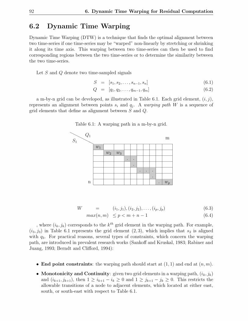
92 6. Dynamic Time Warping for Residual Computation
6.2 Dynamic Time Warping
Dynamic Time Warping (DTW) is a technique that finds the optimal alignment betweentwo time-series if one time-series may be “warped” non-linearly by stretching or shrinkingit along its time axis. This warping between two time-series can then be used to findcorresponding regions between the two time-series or to determine the similarity betweenthe two time-series.
Let S and Q denote two time-sampled signals
S = [s1, s2, . . . , sn−1, sn] (6.1)
Q = [q1, q2, . . . , qm−1, qm] (6.2)
a m-by-n grid can be developed, as illustrated in Table 6.1. Each grid element, (i, j),represents an alignment between points si and qj. A warping path W is a sequence ofgrid elements that define as alignment between S and Q.
Table 6.1: A warping path in a m-by-n grid.
HH
HH
HH
S1
Q1 m
w1
w2 w3
. ..
. . ..
n . wp
W = (i1, j1), (i2, j2), . . . , (ip, jp) (6.3)
max(n,m) ≤ p < m+ n− 1 (6.4)
, where (ik, jk) corresponds to the kth grid element in the warping path. For example,(i3, j3) in Table 6.1 represents the grid element (2, 3), which implies that s2 is alignedwith q3. For practical reasons, several types of constraints, which concern the warpingpath, are introduced in prevalent research works (Sankoff and Kruskal, 1983; Rabiner andJuang, 1993; Berndt and Clifford, 1994):
• End point constraints: the warping path should start at (1, 1) and end at (n,m).
• Monotonicity and Continuity: given two grid elements in a warping path, (ik, jk)and (ik+1, jk+1), then 1 ≥ ik+1 − ik ≥ 0 and 1 ≥ jk+1 − jk ≥ 0. This restricts theallowable transitions of a node to adjacent elements, which located at either east,south, or south-east with respect to Table 6.1.
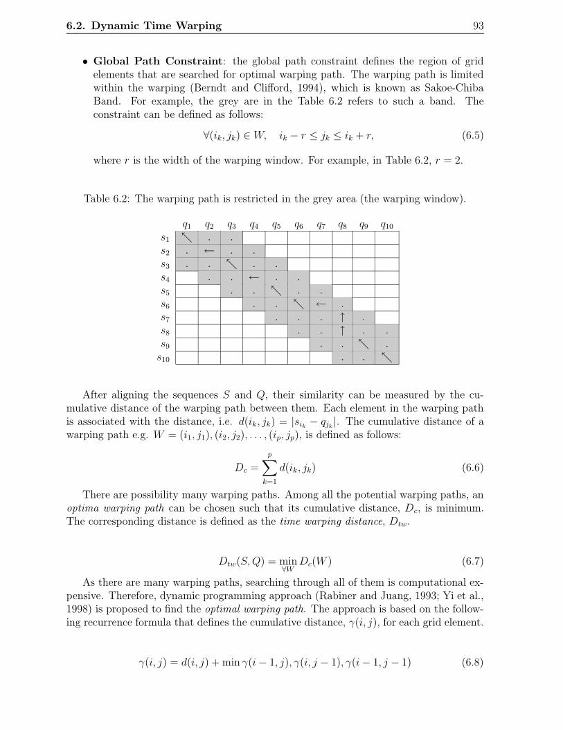
6.2. Dynamic Time Warping 93
• Global Path Constraint: the global path constraint defines the region of gridelements that are searched for optimal warping path. The warping path is limitedwithin the warping (Berndt and Clifford, 1994), which is known as Sakoe-ChibaBand. For example, the grey are in the Table 6.2 refers to such a band. Theconstraint can be defined as follows:
∀(ik, jk) ∈ W, ik − r ≤ jk ≤ ik + r, (6.5)
where r is the width of the warping window. For example, in Table 6.2, r = 2.
Table 6.2: The warping path is restricted in the grey area (the warping window).
q1 q2 q3 q4 q5 q6 q7 q8 q9 q10s1 ↖ . .s2 . ← . .s3 . . ↖ . .s4 . . ← . .s5 . . ↖ . .s6 . . ↖ ← .s7 . . . ↑ .s8 . . ↑ . .s9 . . ↖ .s10 . . ↖
After aligning the sequences S and Q, their similarity can be measured by the cu-mulative distance of the warping path between them. Each element in the warping pathis associated with the distance, i.e. d(ik, jk) = |sik − qjk
|. The cumulative distance of awarping path e.g. W = (i1, j1), (i2, j2), . . . , (ip, jp), is defined as follows:
Dc =
p∑
k=1
d(ik, jk) (6.6)
There are possibility many warping paths. Among all the potential warping paths, anoptima warping path can be chosen such that its cumulative distance, Dc, is minimum.The corresponding distance is defined as the time warping distance, Dtw.
Dtw(S,Q) = min∀W
Dc(W ) (6.7)
As there are many warping paths, searching through all of them is computational ex-pensive. Therefore, dynamic programming approach (Rabiner and Juang, 1993; Yi et al.,1998) is proposed to find the optimal warping path. The approach is based on the follow-ing recurrence formula that defines the cumulative distance, γ(i, j), for each grid element.
γ(i, j) = d(i, j) + min γ(i− 1, j), γ(i, j − 1), γ(i− 1, j − 1) (6.8)

94 6. Dynamic Time Warping for Residual Computation
Illustrative example
Consider two sequences:
S = [2, 5, 2, 5, 2, 1] (6.9)
Q = [0, 3, 6, 0, 6, 0] (6.10)
Table 6.3: A cumulative distance matrix for sequences Q and S.
HH
HH
HH
SQ
0 3 6 0 6 0
2 2 3 7 9 13 155 7 4 4 9 10 152 9 5 8 6 10 125 14 7 6 11 7 122 16 8 10 8 11 91 17 10 13 9 13 10
by applying the dynamic programming algorithm, we can construct a cumulative dis-tance matrix as shown in Table 6.3. Each value in the cell represents the cumulativedistance of that cell. The cumulative distance of a cell is the sum of the distance asso-ciated with it and the minimum of the cumulative distances of its neighboring cells. Forexample:
γ(5, 3) = d(4, 3) + min γ(3, 3), γ(4, 2), γ(3, 2) = 6 (6.11)
After filling up the table, the optimal warping path can be found by tracing backwardfrom the lower right corner, (6, 6), towards the upper left corner, (1, 1). At each cell, wecan choose the previous neighboring cell with minimum cumulative distance.
In the literature review on DTW applications for fault diagnosis we can mention thework done by (Kassidas et al., 1998a) where they used DTW to synchronise batch tra-jectories by combining it with multiway principal component analysis/partial lest squares(PCA/PLS). In (Kassidas et al., 1998b) they reported its use for fault detection and diag-nosis in continuous chemical process, and (Nomikos and MacGregor, 1994) have reportedits use for batch process monitoring.(Li et al., 2004) combined DTW with wavelet decom-position for synchronising batch trajectories. The original signals were decomposed intoapproximations and details at different scales and matched at each scale separately, usingDTW. The matched signals were used, rather that the reconstructed signals, to obtainthe syncronised signal.
In situations with differences in the magnitude of the two signals, DTW would try tosolve the variability in the the Y -axis by warping the X-axis and, thus, result in inap-propriate warping. To overcome this limitation, (Colomer et al., 2002) combined DTW

6.3. On-line Dynamic Time Warping 95
with qualitative representation of signals. Each signal was first decomposed into episodes,which provided a higher-level representation of the signal. DTW was then used to findthe optimal match between the episodes of the two signals, and tested for diagnosis offaults in a level control system.
(Srinivasan et al., 2004) proposed an alternative approach that constraints the searchfor the corresponding points of the two signals, based on landmarks in the signal that arederived from the perspectives of the operators. This constraints were used with DTW.
Above approaches are normally used for off-line applications due to computationalexpensive cost (in both time an memory) of DTW algorithm. In this thesis we propose aslight modification of DTW in order to adapt it for on-line application. Next section isdevoted to explain the main particularities of the new algorithm.
6.3 On-line Dynamic Time Warping
Since DTW is a good method to compensate temporal distortions due to communica-tion delays, this thesis proposes a modification of the algorithm in order to adapt it foron-line application. The new algorithm takes advantage of the warping window in or-der to use it as a sliding window. As main particularities, the two sequences have gotthe same length and the new algorithm returns a distance value at every sample time.So, it is necessary to obtain a finite sequence from original data to calculate new distances.
The algorithm starts at time t = 2 calculating the cumulative distance, γ(i, j) for eachgrid element of the squared matrix. Later on, the matrix grows up and only cumulativedistances for new cells in the matrix are calculated. Next, the matrix reaches a maximumvalue established according to the warping window width, r, and it becomes a sliding win-dow. At each sample time oldest cells in the matrix are deleted and cumulative distancesare calculated for empty cells corresponding to the new sample (figure 6.1). A new pathmust be found for each window and the distance value is obtained calculating the totaldistance according to this new path.

96 6. Dynamic Time Warping for Residual Computation
dn
dn+m
W
W
W
Previously
calculated
values
W
Figure 6.1: On-line DTW.
Illustrative example
Continuing with the example of the previous section 6.2, let’s apply DTWon−line tosequences S and Q, with the width of the warping windows r = 2. Table 6.4 shows thecumulative distance at sample time t = 3, that is when the matrix reaches a maximumvalue established according to the warping window width, r = 2, and it becomes a slidingwindow.
Table 6.5 shows the cumulative distance matrix at sample time t = 4, grids coloredin red denotes cumulative distances computed previously and which not have to be com-puted again, oldest cells (computed at t = 1) are not taken into account and cumulativedistances are calculated just for the new values.
Table 6.4: A cumulative distance matrix for sequences Q and S at the sample time t = 3.
HH
HH
HH
SQ
0 3 6
2 2 3 75 7 4 42 9 5 8

6.3. On-line Dynamic Time Warping 97
Table 6.5: Cumulative distance values of the sliding window for sequences Q and S attime t = 4.
HH
HH
HH
SQ
3 6 0
5 4 4 92 5 8 65 7 6 11
Tables 6.6 and 6.7 show the cumulative distance values of the sliding windows at timet = 5 and t = 6, respectively.
Table 6.6: Cumulative distance values of the sliding window for sequences Q and S attime t = 5.
HH
HH
HH
SQ
6 0 6
2 8 6 105 6 11 72 10 8 11
Table 6.7: Cumulative distance values of the sliding window for sequences Q and S attime t = 6.
HH
HH
HH
SQ
0 6 0
5 11 7 122 8 11 91 9 13 10
Notice that the cumulative distance γ(6, 6) = 10 is the same distance value as ap-plying traditional DTW algorithm. Nevertheless, both methods can not be comparedbecause DTW needs all the sequences S and Q to find an alignment between them, whileDTWon−line uses subsequences of S and Q to find an alignment within the warping win-dow. In any case this fact is a way to confirm that the optimization is going in the rightdirection.
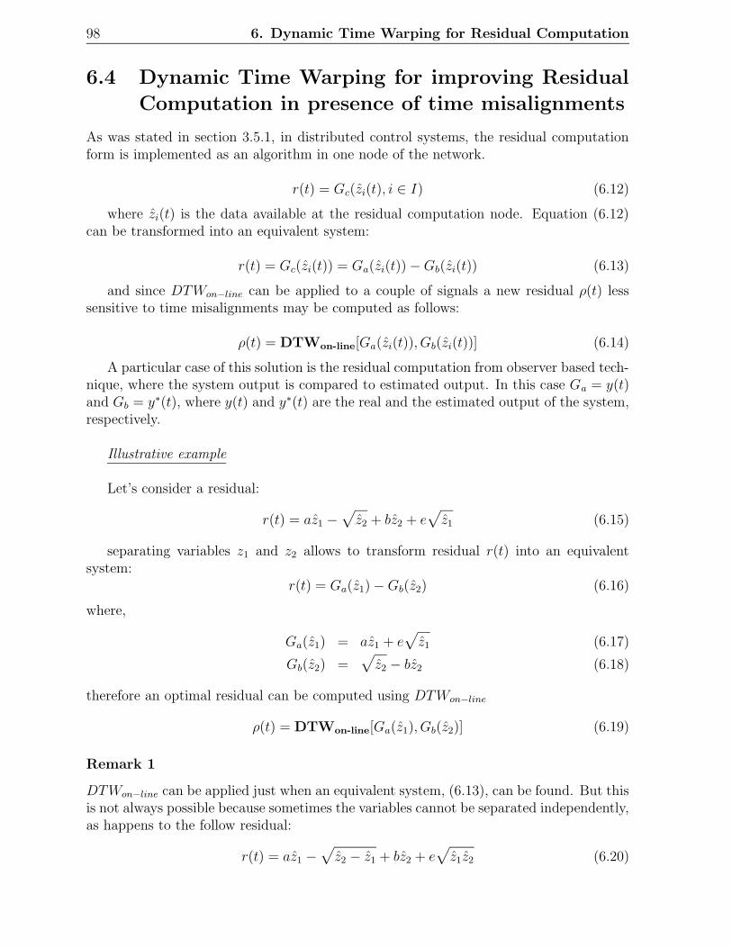
98 6. Dynamic Time Warping for Residual Computation
6.4 Dynamic Time Warping for improving Residual
Computation in presence of time misalignments
As was stated in section 3.5.1, in distributed control systems, the residual computationform is implemented as an algorithm in one node of the network.
r(t) = Gc(zi(t), i ∈ I) (6.12)
where zi(t) is the data available at the residual computation node. Equation (6.12)can be transformed into an equivalent system:
r(t) = Gc(zi(t)) = Ga(zi(t))−Gb(zi(t)) (6.13)
and since DTWon−line can be applied to a couple of signals a new residual ρ(t) lesssensitive to time misalignments may be computed as follows:
ρ(t) = DTWon-line[Ga(zi(t)), Gb(zi(t))] (6.14)
A particular case of this solution is the residual computation from observer based tech-nique, where the system output is compared to estimated output. In this case Ga = y(t)and Gb = y∗(t), where y(t) and y∗(t) are the real and the estimated output of the system,respectively.
Illustrative example
Let’s consider a residual:
r(t) = az1 −√
z2 + bz2 + e√
z1 (6.15)
separating variables z1 and z2 allows to transform residual r(t) into an equivalentsystem:
r(t) = Ga(z1)−Gb(z2) (6.16)
where,
Ga(z1) = az1 + e√
z1 (6.17)
Gb(z2) =√
z2 − bz2 (6.18)
therefore an optimal residual can be computed using DTWon−line
ρ(t) = DTWon-line[Ga(z1), Gb(z2)] (6.19)
Remark 1
DTWon−line can be applied just when an equivalent system, (6.13), can be found. But thisis not always possible because sometimes the variables cannot be separated independently,as happens to the follow residual:
r(t) = az1 −√
z2 − z1 + bz2 + e√
z1z2 (6.20)

6.5. Illustrative example: Fault detection in a NCS laboratory plant 99
Remark 2
Note that missed detections can still occur if a wrong alignment of Ga(zi) and Gb(zi)when a fault is present could conceal its presence in the residual. Nevertheless, this notnecessarily implies a higher missed detection rate. Since it only will occur when thevariation in zi provoked by a fault coincide with previous values of zi. Assuming anadditive model for the fault trace in zi described by zi = zio + zif , being zio the normalexpected value and zif representing the fault, missed detection can appear in presence ofshort faults in specific instants, t, in which the following condition will be satisfied:
zif (t) = −dzio(t)
dt
1
δiδi ≤ ∆ (6.21)
where, δi is the transmission delay and ∆ is its maximum value which is assumed to beknown. Thus, equation 6.21 can be used to provide information of minimum size of faultto be detected according to dynamics of measured variables and behavior of the networkin terms of maximum delay. Moreover, missed detections are intrinsic to the selection ofa neighborhood, N (0), instead of the equality in the evaluation of the residual.
6.5 Illustrative example: Fault detection in a NCS
laboratory plant
6.5.1 Description of the system
The proposed approach has been used on a level control laboratory plant instrumentedwith a networked control and supervisory system. In this plant (See Figure 6.2) a pumpsends liquid from one tank to another one that is placed in a higher level. Water returnsto the first tank by the effect of gravity. A PID control maintains the level in the highertank by governing the pump.
Figure 6.2: Laboratory plant

100 6. Dynamic Time Warping for Residual Computation
The system has been instrumented with sensors (flow-meter and level sensor connectedto a SIEMENS ET200U module) and a PID controller (BURKET 1100) accessible bothvia PROFIBUS as independent nodes. A FDI (Fault Detection and Isolation) modulehas been implemented in a SCADA (Supervisory Control and Data Acquisition) systemrunning in a computer accessing data from an OPC server connected to the PROFIBUSin a master/slave scheme as depicted in Figure 6.3. The time server update cycle (TimeRotation Time) is 137ms.
Network
I/O Module
•SCADA•FDI
PID Controller
Sensor level Flow-meter
Figure 6.3: Process communication
The availability of data in the OPC-client computer has been tested under differentconditions of refreshing time (Sample time) and number of devices.
Figure 6.4a) represents the histograms of delays of the monitored process variableswith a sample time of 100ms. Delays were calculated as the difference between times-tamps labelled by the OPC server. Samples located close to zero denotes repeated data,which means that the server did not have time to update the value. Samples around100ms represent data arriving on time and samples on the right of the histogram indicatedelayed data.
While for histogram of figure 6.4b), delays are insignificant compared to the sampletime (1000ms). In that situation is guaranteed that the refreshing time in the OPC-clientcomputer will coincide with OPC server updates.
It can be concluded that sample time and timestamp not are always coincident andobviously delays and misalignments increase as sample time decreases nearly to the targetrotation time. In order to emphasize this source of errors residual computation has beenevaluated under these circumstances.

6.5. Illustrative example: Fault detection in a NCS laboratory plant 101
0 50 100 150 200 2500
10
20
30
40
50
60
a) Delay (ms)
Sam
ples
980 990 1000 1010 10200
50
100
150
200
250
300
350
b) Delay (ms)
Sam
ples
Figure 6.4: Histograms of delays of the monitored process variables a)Ts=100msb)Ts=1000ms.
6.5.2 Results
Applying the structural analysis technique (Blanke et al., 2003) the following computa-tional forms for the residuals (See details in Appendix C):
r1 = QP − k1
√
h3 − 13− k2
√
h3 − 7, 5− Ah3 (6.22)
r2 = k1
√
h3 − 13 + k2
√
h3 − 7, 5− k3
√
h2 − Ah2 (6.23)
r3 = u(t).QP −QP (6.24)
where QP , h2 and h3 are the monitored process variables that represent the input flowinto the tank 3, the level of thank 2 and the level of tank 3, respectively; all the monitoredprocess variables are affected by the communication delays. A is the cross section area ofthe tanks and k1, k2 and k3 are known parameters.
Residuals must be evaluated at anytime with values of process variables acquired atthe same time. Typically a sampling time is defined to evaluate periodically the consis-tency of data coming from process. This periodicity also facilitates the computation ofderivatives involved in the relations, i.e. r2. Derivative calculation is done by subtractingthe output value at the previous time step from the current value, and dividing by thesample time.
In order to see how misalignments affect residual r2, a sample rate of 100ms has beenfixed as a periodic interval to compute the redundancy equations. Decision thresholdshave been determined as x± 3σ , where x is the mean and σ is the standard deviation.

102 6. Dynamic Time Warping for Residual Computation
0 5 10 15
x 104
−0.4
−0.2
0
0.2
0.4
a) ms
0 5 10 15
x 104
−0.01
−0.005
0
0.005
0.01
0.015
b) ms
Figure 6.5: a) r2 and b) ρ2 using DTWon−line.
Figure 6.5a) depicts the implementation of r2 and it can be seen some values thatcross the thresholds, which might lead to false alarms.
In order to apply DTWon−line, r2 has to separate in two signals:
Ga(h3) = k1
√
h3 − 13 + k2
√
h3 − 7, 5 (6.25)
Gb(h2) = k3
√
h2 − Ah2 (6.26)
using DTWon−line the r2 can be computed as follows:
ρ2 = DTWon−line(Ga(h3), Gb(h2)) (6.27)
Figure 6.5b) shows how DTWon−line reduces the number of false alarms. The warpingwindow size has been configured in 40 samples.
6.5.3 Time consuming
Table 6.8 resumes the time consuming comparison of two sequences using DTW andDTWon−line. Algorithms implementation were done in a 2.4 GHz Pentium 4 with 512 MBof RAM. The computation of the cumulative distance matrix is the most consuming timefactor of both methods, however since DTWon−line uses previously calculated it is fasterthan DTW.

6.6. Conclusions 103
Table 6.8: Time consuming comparison between DTW and DTWon−line
Method Warping window Cumulative distance Pathwidth time consuming time consuming
DTW 40 1.1 s 1 msDTWon−line 40 20 ms 1 ms
6.6 Conclusions
In this chapter, an approach based on classic DTW was developed to be used online inorder to obtain residuals from a laboratory plant. This approach is specially suitable forthose errors related with time distortions. Therefore, it will be useful for distributed sys-tems with communication delays and for hybrid systems with on/off sensors or actuatorscausing misalignments between real and simulated signals.
The results show a hight robustness for on-line DTW. In fact, the results obtainedevidenced less false alarms using on-line DTW than a normal implementation.
As restrictions, the new approach continues using dynamic programming and it couldbe computationally expensive depending on considerations as number of variables, warp-ing window width, sample time or computer effort.

104 6. Dynamic Time Warping for Residual Computation

Chapter 7
Time Misalignment Reduction inSymptom Based Diagnosis
7.1 Introduction
In non model based fault diagnosis the deterministic model given by analytical equationsare not available anymore. The only information we have from the process are the inputu(t) and the output y(t) signals represented as a time-series which are a rich source in-formation that can be used for diagnosis purpose.
A symptom is a subjective evidence of a fault that indicates the existence of a fault,then symptom based method allows a forward reasoning from fault to possible faults.This method can be performed with different techniques: fault trees, heuristics (rules),knowledge about process history (cases), statistical knowledge (belief networks), classifi-cation (neural network), expert systems, Case Based Reasoning.
Case Based Reasoning (CBR) is a problem solving methodology based on the reuse ofprevious experiences. The basic idea is focused on the hypothesis that ”similar problemshave similar solutions” (Wilke and Bergmann, 1998). CBR methodology proposes a four-step cycle (Retrieve, Reuse, Revise and Retain) also known as the 4R-cycle. It basicallyconsists in Retaining experiences as cases for a further Reuse (submitted to a Revisionprocedure). Cases are registers containing a description of a problem ”symptoms” andits solution ”diagnostic”. The aim is to reuse these cases for solving new problems byanalogy. In presence of a new problem, the basic procedure consists of Retrieving ana-logue cases, according to their description (attributes defining symptoms), and reusingtheir solutions (diagnostic).
When cases are represented by time series, searching within a time series database forthose series that are similar to a given query sequence is very important during the Re-trieve step. Time misalignments may produce erroneous results when this task is carriedout.
In this chapter Dynamic Time Warping (DTW) is proposed as a similarity criteria toimplement the retrieval task, with the aim to reducing the influence of time-misalignments.
105

106 7. Time Misalignment Reduction in Symptom Based Diagnosis
An electrical system problem, known as voltage sag, has been used to test the proposedmethod, (Llanos et al., 2003a; Melendez et al., 2004a; Llanos et al., 2004b).
The chapter is organized as follows: Section 7.2 presents the methods of Case BasedReasoning (CBR). The efect of time misalignments while performing the Retrieving taskis analysed in Section 7.3. Proposed solution using DTW is described in Section 7.5. TheIllustrative example is shown in Section 7.6. Finally some concluding remarks are givenin Section 7.7.
7.2 Case Based Reasoning
Case Based Reasoning is an approach to problem solving that is able to use specificknowledge of previous experiences (Lopez and Plaza, 1997). A new problem is solved bymatching it with a similar past situation. If the problem is solved, this new situation willbe retained in order to solve other new ones. In the case of diagnosis, solving the problemmeans that the CBRsystem proposes a solution that is satisfactory enough to identify thenew fault.
Many authors have discussed about, the appropriate situations where CBR offersadvantages. In (Main et al., 2001) many of these advantages were summarized and theorder in which they appear here is not indicative of their level of importance:
• Reduction of the knowledge acquisition task: by eliminating the extraction of modelor set of rules as is necessary in model/based reasoning.
• To avoid repeating mistakes made in the past: system can use the information aboutwhat caused faults in the past to predict any faults in the future.
• Graceful degradation of performance: some model based systems cannot even at-tempt to solve a problem on the boundaries of its knowledge or scope, or whenthere is missing or incomplete data. In contrast case based systems can often havea reasonably successful attempt at solving these types of problem.
• To be able to reason in domains that have not been fully understood, defined ormodelled: CBR can deal with only a set of cases from the domain.
• To be able to make predictions: the reasoner may be able to predict the success ofthe suggested solution to a current problem. This may be done by referring to thestored solutions and to the differences between the previous and current solutioncontext.
• To learn over time: if cases are tested in the real world an level of success deter-mined, there cases can be added into the case base to reason with it in future.
• To reason in a domain with small body of knowledge: a case based reasoner canstart with a few known cases and incrementally increase its knowledge as cases areadded to it.

7.3. CBR cycle 107
• To reason with incomplete or imprecise data and concepts: as cases are retrieved notjust when identical to the current query case but also when they are within somemeasure of similarity, incompleteness and imprecision can be deal with. Whilethese factors may cause a slight degradation in performance due to the current andretrieved having increased disparity, reasoning can still continue.
• Avoid repeating all the steps that need to be taken to arrive at a solution: by reusinga previous solution, the steps taken to reach the retrieved solution can be reusedthemselves.
• Provide a means of explanation: by explaining how a previous case was successfulin a situation, using the similarities between the cases and the reasoning involvedin adaptation a CBR systems can explain its solution to a user
• Can be used in different ways: CBR can be used for many purposes as for creatinga plan, making a diagnosis, arguing a point of view, etc.
• Reflects human reasoning: humans can understand a CBR system’s reasoning andexplanations and are able to be convinced of the validity of the solutions they arereceiving.
7.3 CBR cycle
(Aamodt and Plaza, 1994) have described CBR as a cyclical process comprising the fourREs. It basically consists in Retaining experiences as cases for a further Reuse. Casesare registers containing a description of a problem and its solution. The aim is to reusethese cases for solving new problems by analogy. In presence of a new problem, the basicprocedure consists of Retrieving analogue cases and reusing their solutions. Reuse im-plies an adaptation procedure of the retrieved solutions that is finished with a Revision.After validation, the cycle is completed by Retaining the solved situation (problem + newsolution). In practice it is often confused the separation between reuse and revise and itis common to merge both in one operation named adaptation. The procedures involvedin CBR can be represented by a schematic cycle, see Figure 7.1.
Cases are stored according to a suitable structure, named case memory, into case baseswhere indexing mechanisms are used for an efficient retrieval. CBR foundations and adetailed description of this methodology based on the 4R are wider described in (Aamodtand Plaza, 1994; Langseth et al., 1999). Next the four stages depicted in Figure 7.1 aredescribed.
7.3.1 Retrieval
The Retrieval of cases is closely related and dependent on the indexing methods used.In general, several techniques are currently used: nearest-neighbor retrieval, inductiveretrieval, knowledge guided approaches and validated retrieval.
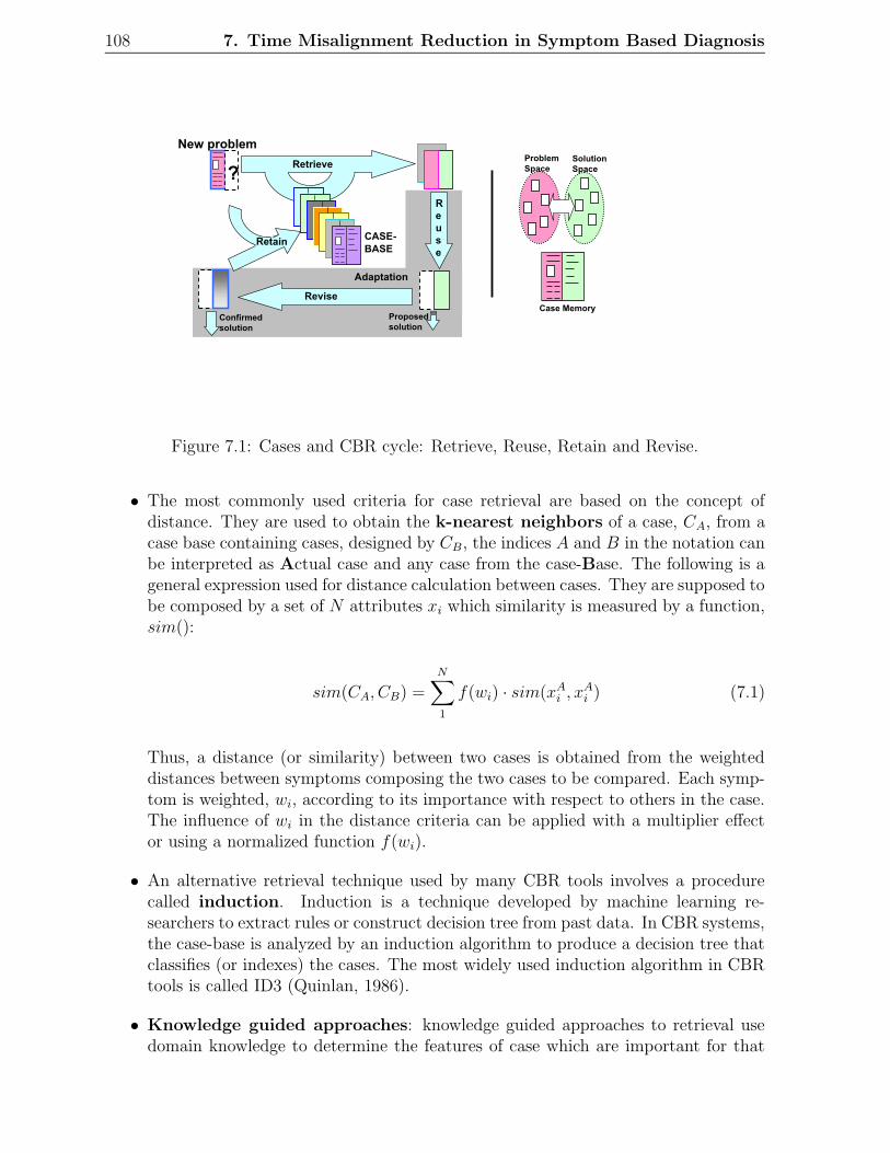
108 7. Time Misalignment Reduction in Symptom Based Diagnosis
New problem
CASE-
BASE
Revise
Proposed
solutionConfirmed
solution
?Retrieve
Retain
R
e
u
s
e
Adaptation
Case Memory
Problem
SpaceSolution
Space
Figure 7.1: Cases and CBR cycle: Retrieve, Reuse, Retain and Revise.
• The most commonly used criteria for case retrieval are based on the concept ofdistance. They are used to obtain the k-nearest neighbors of a case, CA, from acase base containing cases, designed by CB, the indices A and B in the notation canbe interpreted as Actual case and any case from the case-Base. The following is ageneral expression used for distance calculation between cases. They are supposed tobe composed by a set of N attributes xi which similarity is measured by a function,sim():
sim(CA, CB) =N
∑
1
f(wi) · sim(xAi , x
Ai ) (7.1)
Thus, a distance (or similarity) between two cases is obtained from the weighteddistances between symptoms composing the two cases to be compared. Each symp-tom is weighted, wi, according to its importance with respect to others in the case.The influence of wi in the distance criteria can be applied with a multiplier effector using a normalized function f(wi).
• An alternative retrieval technique used by many CBR tools involves a procedurecalled induction. Induction is a technique developed by machine learning re-searchers to extract rules or construct decision tree from past data. In CBR systems,the case-base is analyzed by an induction algorithm to produce a decision tree thatclassifies (or indexes) the cases. The most widely used induction algorithm in CBRtools is called ID3 (Quinlan, 1986).
• Knowledge guided approaches: knowledge guided approaches to retrieval usedomain knowledge to determine the features of case which are important for that

7.3. CBR cycle 109
case in particular to be retrieved in future. In some situations different features ofeach case will have been important for the success level of that case.
• Validated retrieval (Simoudis, 1992), consists of two phases, firstly the retrievalof all cases that appear to be relevant to a problem, based on the main featuresof query case. The second phase involves deriving more discriminating featuresfrom the group of retrieved cases to determine whether they (cases) are valid in thecurrent situation. The advantage of this method is that inexpensive methods canbe used in the second phase as they are applied to only a subset of the case-base.
7.3.2 Reuse
Once a matching case is retrieved, a CBR system will attempt to Reuse the solutionsuggested by the retrieved case. In many circumstances the solution may be sufficient.However, in other instances the solution from the retrieved case may be close to therequired solution, but no close enough. The CBR system must then adapt the solutionstored in the retrieved case to the needs of current case. Adaptation looks for prominentdifferences between the retrieved case and the current case and then applies rules that takethose differences into account when suggesting a final solution. There are two principalmethods to reuse (or adapt) past cases (Allemang, 1994):
• Transformational reuse: which consists of reusing past solutions. The retrievedcase solution is not the solution adopted for the new problem, rather there is atransformation function that generates the new solution from past cases.
• Derivational reuse: this consists of reusing the procedure followed to deducethe past solutions. In this approach, the retrieved case must contain informationabout the method used for solving the retrieved problem, including a justificationof the operations used, their subgoals, alternatives generated, failed search paths,etc. Derivational reuse reruns the retrieved method with the new case details andreplays the old plan into the new context.
7.3.3 Revise
In this phase the proposed solution is analyzed to assess its accuracy. The proposed so-lution (generated in Reuse) is evaluated, and if the solution is successful, the CBR canlearn from it as will be shown in the next phase (case Retention); if the solution is notsuccessful it can be repaired using domain specific knowledge. Evaluating a solution isnormally done by applying the solution to a real world problem. Under some circum-stances, the solution can be evaluated using a simulation. If the proposed solution needsto be repaired, it is necessary to identify the errors in the solution and to generate anexplanation for them, using techniques that allows to repair errors.
7.3.4 Retain
The power of CBR is based on the richness of the case-base; therefore it is important toretain new cases and its solution. In this phase of the CBR cycle it is determined what

110 7. Time Misalignment Reduction in Symptom Based Diagnosis
can be learned and retained from a problem solving episode. The learning algorithmmust take into account the outcome of the previous phase of the CBR cycle. The mainsub-tasks of this step are:
• Selecting which information must be retained
• Establishing how this information must be saved
• Establishing how to index the new problem solving episode (case) for future re-trievals
• Determining how to integrate the new case in the memory structure
7.4 Effects of time misalignment in case retrieval
7.4.1 Cases represented as time-series and experience
The conceptual definition of cases, considered in CBR, allows performing an associationbetween two complementary views of process behaviour. One of them is provided byacquisition systems as flows of data that are systematically collected and stored. Theother view is the human perception of process behaviour enhanced by the expertise andexperience. They are two different views of the same reality (Langseth et al., 1999), theprocess, which must be combined in order to improve the global knowledge of processneeded in assessment tasks. According to this premise, cases are conceived as knowledgecontainers that perform the association between both: C = [S(t), D]: where S(t) repre-sents symptoms that characterise the situations under study and D reflects the operatorexperience (diagnosis, hypothesis, etc). Symptoms are representations of acquired signalsobtained directly from data or after an abstraction procedure. The expert view encap-sulated in D represents the evaluation (diagnosis) of the given situation, a set of actionsto perform under determined situation or similar information needed to preserve processunder normal operation conditions or for warning operator in posterior similar situations.
In this Chapter symptoms are represented as time-series obtained directly from thesystem output y(t) during a time window [ti, tf [. Therefore a case is defined as:
C = [y(t), D] (7.2)
7.4.2 Time misalignment in case retrieval
As was introduced above in subsection 7.3.1, the most commonly used criteria for caseretrieval are based on the concept of distance. Most of algorithm that operate withtime-series of data use the Euclidean distance or some variation. However, Euclideandistance could produce an incorrect measure of similarity because it is very sensitive todistortions in the time axis (time misalignments). Therefore, robust yet sensitive methodsfor comparing unsynchronized signals are an active area of research.

7.5. Dynamic time warping for case retrieval 111
7.5 Dynamic time warping for case retrieval
Since Dynamic Time Warping is a good method to compensate temporal distortions onthe time axis, in this chapter it is proposed to use it as a distance criteria for case retrieval.Therefore applying DTW to (7.1), produces the similarity function:
sim(CA, CB) = DTW(yA(t), yB(t)) (7.3)
Thus, a distance (or similarity) between two cases (CA, CB) is obtained from DTWbetween theirs corresponding symptoms (yA, yB). Once a matching case is retrieved, aCBR system will attempt to Reuse the solution (D) suggested by the retrieved case.
7.6 Application in an Electrical System: diagnosis of
voltage sags in a 25kV substation
Electrical energy is supplied in form of a three-phase voltage of sinusoidal nature. Thereare four parameters that characterise the voltage wave, allowing measuring its degree ofquality. These parameters are: frequency, amplitude, shape and symmetry. Electricalpower stations produce a sine wave of 50 or 60 practically perfect cycles per second.
However, during the energy transport and distribution from the generation substa-tion to the final customer, these parameters can suffer alterations which affect the wavequality. These alterations could have their origin in the electrical facility (as a result ofbreaker switching, failures, and so on), in natural phenomena, operation of loads (recti-fying bridges, arc furnaces, and so on), or others. This alteration of the sinusoidal waveis usually transmitted to the electrical system (Bollen, 2000).
7.6.1 Voltage sag definition
An alteration defined in power systems is known as voltage sag. Standard definition(Bollen, 2000) of sags is based on the minimum rms value obtained during the event andits duration is the time interval between the instant when rms voltage crosses the voltagesag threshold (usually 90% of normal voltage) and the instant when it returns to normallevel. A three-phase unbalanced voltage sag is shown in Fig. 7.2.
7.6.2 Cases represented by voltage magnitude and location
In order to establish a similarity criteria among the voltage sags, a technique proposedin (Bollen, 2000) to characterise them has been used. This technique allows a characteri-sation through a one complex voltage. The method is based on the decomposition of thevoltage phasors in symmetrical components (Grainger and Stevenson, 1998). The three(complex) phase voltages in an unbalanced (not all three phases have the same magnitudeor 120o between them) system can be completely described through three component volt-
ages, known as symmetrical components. Positive-sequence voltage ~V1, negative-sequencevoltage ~V2 and zero-sequence voltage ~V0 are calculated from the complex phase voltagesas follows:

112 7. Time Misalignment Reduction in Symptom Based Diagnosis
0 5 10 15
-1
-0.5
0
0.5
1
Time in cycles
Voltage in p
u
0 5 10 150
0.2
0.4
0.6
0.8
1
1.2
Time in cycles
Voltage in p
u
a) b)
Figure 7.2: a)Example of a three-phase voltage sag b) rms voltage
~V0
~V1
~V2
=1
3
1 1 11 a a2
1 a2 a
where
a = −1
2+
1
2j√
3 (7.4)
The characteristic voltage, ~V , indicates the severity of the sag, it is obtained from:
~V = ~V1 − ~V2
′
(7.5)
The voltage magnitude is a time-series defined as the absolute value of the character-istic voltage:
V =| ~V | (7.6)
Voltage sag magnitude, V , is used as symptom on the case representation. Theevaluation (diagnosis) of the given situation is represented by the electrical location of thefault, L, namely distribution or transmission. Therefore a case may be representedby the double:
S = (V (t), L) (7.7)
7.6.3 Dynamic Time Warping for voltage sag retrieval
Given two sags SA and SB described by their characteristic voltage VA and VB, respec-tively, the idea is to use DTW as a metric to define similarities between them:
sim(SA, SB) = DTW (VA(t), VB(t)) (7.8)

7.6. Application in an Electrical System: diagnosis of voltage sags in a 25kVsubstation 113
a)
b)
Figure 7.3: Voltage sag classification: a)Distribution b)Transmission.
7.6.4 Results
Spanish Electrical Facility (Endesa Distribution SL) has provided voltage sags in a 25kVdistribution substation. 550 voltage sags were recorded and chosen to apply this method.500 sags (of the recorded ones) were used for the creation of the case-base, they were sep-arated in two groups according to the location of the fault (transmission/distribution):360 voltages sags (72%) caused by fault in transmission systems and 140 voltage sags(28%) caused by faults in distribution systems. The 50 remaining voltages sags were usedas new cases to be diagnosed.
Figure 7.3a) and 7.3b) show, respectively, the typical voltage sag wave forms accord-ing to the location of the fault, transmission or distribution. The rms voltage of thecharacteristic voltage sag is depicted on the right side of the figures. The rms voltage ofthe three phases are depicted on the left side of the figures. The rms voltage of the threephases were used in order to obtain the so called temporal attributes, (Llanos et al., 2003b;Mora et al., 2003a), temporal attributes are quantitative values such as magnitude, peaks,slopes and voltage sag duration. Temporal attributes are described in details in AppendixD.
In order to compare the results of DTW, two more distances criteria were also applied.One based on Euclidean distance, which also uses the time-series representation of thecharacteristic voltage, V (t). And the other criteria was the Manhattan distance which isapplied to the so called temporal attributes.
DTW is the less sensitive distance approach to the time misalignment. Table 7.1shows the diagnostic error after applying the three above distance approaches to the 50new cases.

114 7. Time Misalignment Reduction in Symptom Based Diagnosis
Table 7.1: Diagnostic error using Euclidean, Manhattan and DTW distances
Euclidean Manhattan DTWDiagnostic error 22% 16% 8%
Figure 7.4: Two similar characteristic voltage sags. a) The Euclidean distance, b) DTW.
Figure 7.4a) shows the intuitive alignment produced by Euclidean distance. Bothshapes have the same magnitude but they have been moved on the y-axes in order toshow the alignment allowed by the two methods. The lines between the shapes show thepoint that is been compared in each waveform. Euclidean distance produces a pessimisticresult of similarity since the signals are not aligned in time. While, Figure 7.4b) showshow DTW finds an alignment that allows a correct measure of similarity.
Figure 7.5 shows a new case that have not been well diagnosed using DTW. The wave-form is more similar to a transmission voltage sag than a distribution one, but DTW givesa contrary result. It is because in this method magnitude is more relevant than voltageduration time.
The crucial observation is that the algorithm may try to explain variability in theY-axis by warping the X-axis. This can lead to unintuitive alignments where a singlepoint on one time series maps onto a large subsection of another time series.
The weakness of DTW is in the features it considers. It only considers a data pointsY-axis value. For example if we consider two data points (xi and yj) which have identicalvalues, but (xi) is part of a rising trend and (yj) is part of a falling trend. DTW considersa mapping between these two points ideal, although intuitively we would prefer not tomap a rising trend to a falling trend.
To prevent this problem, in (Keogh and Pazzani, 2001), a modification of DTW that
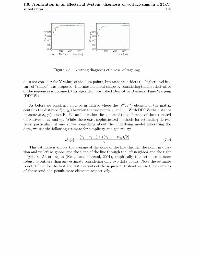
7.6. Application in an Electrical System: diagnosis of voltage sags in a 25kVsubstation 115
Figure 7.5: A wrong diagnosis of a new voltage sag.
does not consider the Y-values of the data points, but rather considers the higher level fea-ture of ”shape”, was proposed. Information about shape by considering the first derivativeof the sequences is obtained; this algorithm was called Derivative Dynamic Time Warping(DDTW).
As before we construct an n-by-m matrix where the (ith, jth) element of the matrixcontains the distance d(xi, yj) between the two points xi and yj. With DDTW the distancemeasure d(xi, yj) is not Euclidean but rather the square of the difference of the estimatedderivatives of xi and yj. While there exist sophisticated methods for estimating deriva-tives, particularly if one knows something about the underlying model generating thedata, we use the following estimate for simplicity and generality:
Dx[x] =(xi − xi−1) + ((xi+1 − xi11)/2)
2(7.9)
This estimate is simply the average of the slope of the line through the point in ques-tion and its left neighbor, and the slope of the line through the left neighbor and the rightneighbor. According to (Keogh and Pazzani, 2001), empirically this estimate is morerobust to outliers than any estimate considering only two data points. Note the estimateis not defined for the first and last elements of the sequence. Instead we use the estimatesof the second and penultimate elements respectively.

116 7. Time Misalignment Reduction in Symptom Based Diagnosis
7.7 Conclusions
This chapter proposes the use of Dynamic Time Warping (DTW) for reducing the effectsof time misalignment when Case Based Reasoning (a symptom based diagnosis) is per-formed. DTW is used as a similarity criteria to implement the retrieval task.
An electrical system problem, known as voltage sag, has been used to test the pro-posed method.
In order to compare the results of DTW, two more distances criteria were also applied.One based on Euclidean distance, which also uses the time-series representation of thecharacteristic voltage. And the other criteria was the Manhattan distance which has beenapplied to the temporal attributes. Results shows that DTW is the less sensitive distanceapproach to the time misalignment.

Chapter 8
Conclusions and Future Work
In the following paragraphs, the main aspects of the contributions of the present thesisare considered:
• Fault Detection and Diagnosis (FDD) deal with the timely detection, diagnosis andcorrection of abnormal conditions of fault in a process. To accomplish these tasks,all the process knowledge (structure, dynamic and static equations, parameters,heuristic knowledge, etc) and measured data from the process variables, have to beused. But these two sources of information carried several problems such as knowl-edge acquisition and representation, measurement noise, modelling uncertainties,time misalignment between measured data, among others. This thesis is focused onthe study of time misalignments effects when performing FDD.
• As networks continue to built out, and network technology becomes cheaper andmore reliable than traditional fixed point-to-point wiring connections, more andmore control systems have operated and will operate over networks. In this case,the sensor, the actuator, diagnostic, command and coordination signals are all trav-elling over common networks. Feedback control systems with at least one loop closedthrough data networks are called distributed control systems (DCS). In distributedcontrol systems, the residual computation form is implemented as an algorithm inone node of the network. In the literature review of FDI in DCS it is proposed themodification of the system model in order to deal with communication delays anddata dropout. This thesis proposed a solution for time-delays and data dropout ef-fects in DCS when performing FDI, the solution does not modify the system model.Our firsts studies of time misalignment are published in (Llanos et al., 2005; Llanoset al., 2004a).
• In this thesis it is shown that when transmission delays are known, it is possibleto take them into account in the residual computation, thus introducing a delayedbut otherwise unchanged decision and avoiding false alarms due to delays. However,when delays are unknown it is necessary to estimate them in order to compensate fortheir effect in the decision procedure. In this case, based on a very rough model of
117

118 8. Conclusions and Future Work
the delays, the problem is addressed as an optimization problem. A search algorithmis used for the delay estimation by minimizing the residual under the constraintsgiven by the transmission model. When the persistent excitation condition is ful-filled, the delays estimation can be carried out giving reliable results and avoidingfalse alarms. The efficiency of the proposed approach has been applied on a controlposition for a DC motor. Results are published in (Llanos et al., 2007; Llanos et al.,2006).
• A simple formulation has been proposed to solve the problem of data dropout whenperforming FDI. It is based on the computation of the residual with the availabledata at each time instant instead of using the classical formulation. The principalbenefit is the drastic reduction of false alarm ratio avoiding the classical trade offwith missed detection. The efficiency of the proposed approach is illustrated ona laboratory plant, where the false alarms during the transient time window werereduced without increasing the missed detections under different conditions of datadropout.
• Another solution to the problem of time misalignment has been proposed. It isbased on the Dynamic Rime Warping (DTW) algorithm. DTW is a technique thatfinds the optimal alignment between two signals. DTW is computationally expen-sive (in both time an memory) because it uses dynamic programming, therefore itis normally used for off-line applications. In this thesis we proposed a slight mod-ification of DTW in order to adapt it for on-line application. The results show ahight robustness for on-line DTW. In fact, the results obtained evidenced less falsealarms using on-line DTW than a normal implementation. Results are published inGamero et al., 2004; Llanos et al., 2004b).
• The non model based techniques, that use the comparison and matching of signalsfor performing fault diagnosis, can also be affected by time misalignments becausemost of the algorithms, that operate with time-series of data, use the Euclideandistance or some variation. Euclidean distance could produce an incorrect measureof similarity because it is very sensitive to distortions in the time axis. This thesisproposed the use of DTW for reducing the effects of time misalignment when CaseBased Reasoning (a symptom based diagnosis) is performed. DTW is used as asimilarity criteria to implement the retrieval task. An electrical system problem,known as voltage sag, has been used to test the proposed method. In order tocompare the results of DTW, two more distances criteria were also applied: Onebased on the Euclidean distance, which also uses the time-series representation andthe Manhattan criterion. The results show that DTW is the least sensitive distanceapproach to the time misalignment. Results are published in (Melendez et al., 2004a;Llanos et al., 2004b; Llanos et al., 2003a; Llanos et al., 2003b; Mora et al., 2003a;Mora et al., 2003c; Melendez et al., 2003; Mora et al., 2003b).

119
Some research topics that can be studied in the future are discussed as follows:
• In order to consider the dynamic of the residual generator, any observer based resid-ual generator could be used when analyzing the impact of network delay in residualgeneration.
• In this thesis the network communication model was modelled by a very simpledeterministic model. It will be interesting to model phenomena as network queues,varying network loads, measurement noise and others peculiarities of networks thatcould degrade the performance of the fault diagnosis system.
• In this thesis the effects of time misalignments when performing fault isolation hasnot been analyzed. It would be interesting to analyze what happens to the signa-ture matrix and even if its possible to design structured residuals sensitives to thenetwork communication problems.
• The on line DTW approach continues using dynamic programming and it couldbe computationally expensive depending on considerations such as the number ofvariables, warping window width, sample time or computer effort. Future work canbe done in order in to introduce restrictions that would allow reducing the effectsof the above mentioned considerations.
• Another weakness of DTW is in the features it considers. DTW only takes intoaccount a data points Y-axis value. In order to deal with this situation, in (Keoghand Pazzani, 2001), a modification of DTW that does not consider the Y-valuesof the data points, but rather considers the higher level feature of “shape”, wasproposed. This algorithm was called Derivative Dynamic Time Warping (DDTW).The next step should be to adapt DDTW in order be used on-line.

120 8. Conclusions and Future Work

Appendix A
Design of the analytical redundancyrelation of a control position for aDC motor
From Figure A.1 the following equations can be written based on Newton’s law combinedwith Kirchhoff’s law:
Raia(t) +K3dc(t)
dt= K0K1e(t) (A.1)
Dd2c(t)
d2t+ b0
dc(t)
dt= K2ia(t) (A.2)
where,K0, K1, K2, K3, b0, D and Ra are known parameters and, e(t) and c(t), are mea-surements available from the process.
u
Figure A.1: Schematic diagram of a control position for a DC motor.
121

122A. Design of the analytical redundancy relation of a control position for a
DC motor
Table A.1: Incidence matrix.
↗ ia e c c c
c1 1 1 1
c2 1© 1
d3 1©d4 1©m1 1©m2 1©
Next equations describe the operation mode of the system:
c1 : e(t) =Raia(t) +K3
dc(t)dt
K0K1
(A.3)
c2 : ia(t) =D d2c(t)
d2t+ b0
dc(t)dt
K2
(A.4)
d3 : c(t) =dc(t)
dt(A.5)
d4 : c(t) =d2c(t)
d2t(A.6)
m1 : c(t) = cm1(A.7)
m2 : e(t) = em2(A.8)
Redundancy relations have been obtained from the following matching Table A.1 usingthe ranking algorithm described in (Blanke et al., 2003). The corresponding orientedgraph is shown in figure C.1.
Simplifying the operation model equations using the matched variables results in the
c
Zeroc1
d3
m2c2•c
••c
d4
ia
em1
Figure A.2: Oriented structure graph of the system

123
following redundancy relation:
r(t) = Dd2c(t)
dt2+B
dc(t)
dt−Ke(t) (A.9)
whit,
B = b0 +K2K3
Ra
(A.10)
K = K0K1K2 (A.11)

124A. Design of the analytical redundancy relation of a control position for a
DC motor

Appendix B
Design of the analytical redundancyrelations of the laboratory plant
Next equations describe the model of the laboratory plant, see Figure B.2:
c1 : Qi = u.Qi (B.1)
c2 : Qo = K.√h (B.2)
d3 : h =d
dth (B.3)
c4 : h =1
A(Qi −Qo) (B.4)
m1 : h = hm1(B.5)
m2 : Qi = Qi,m2(B.6)
where h, Qi and Qo are the level, the input and the output flow to the higher tank,respectively. u is the control signal and Qi is a parametrization of the pump. A andK are known parameters. m1 and m2 are additional measurement constraints given bythe flow-meter and the level sensor. Redundancy relations have been obtained from thefollowing matching table (Table B.1) where the ’1’ indicates the presence of the variable(columns) in the equation (rows). The ranking algorithm described in (Blanke et al.,2003) has been used to obtain the ’zero ’ or redundancy equations. Circles indicate theselected variables in the iterative ranking procedure. The corresponding oriented graph(Figure B.1) shows how equation c1 and c4 are the basis for the two ARR.
Simplifying the operation model equations using the matched variables results in thefollowing residuals:
r1 = Qi −K√h− Ah = 0 (B.7)
r2 = u.Qi −Qi = 0 (B.8)
After a simple discretisation (unitary sample time) of variables and derivatives thecomputation equation of residuals are the following:
r1(k) = Qi(k)−K√
h(k)− A(h(k)− h(k − 1)) = 0 (B.9)
125

126 B. Design of the analytical redundancy relations of the laboratory plant
Table B.1: Incidence matrix.
↗ Qi Qo h hc1 1c2 1© 1d3 1 1©c4 1 1 1m1 1©m2 1©
c1
Qi
Qoh
h
u
Zeroc4 c2
d3
m1
m2 Zero
Figure B.1: Oriented structure graph of the system.
r2(k) = u(k).Qi −Qi(k) = 0 (B.10)
TANK
Driver
TANK
PID controller
Pump
Level Sensor
Flow-meter
Figure B.2: Image of the laboratory plant.

Appendix C
Design of the analytical redundancyrelations of the three tanks system
Next equations describe the model of the laboratory plant, see Figure C.2. Valves V9 andV10 are located 13cm and 7.5cm, respectively, from the bottom of thanks. Dependingon the water levels there exist several different operation modes for the system. As apractical example, level in TANK 3 has been maintained in 20cm and TANK 2 in 7cm.Next equations describe the operation mode for the system:
c1 : QL = 0 (C.1)
c2 : QP = u(t).QP (C.2)
c3 : h3 =1
A(QP −QL −Q32) (C.3)
d4 : h3 =d
dth3 (C.4)
c5 : Q32 = k1
√
|h3 − 13|+ k2
√
|h3 − 7, 5| (C.5)
d6 : h2 =d
dth2 (C.6)
c7 : h2 =1
A(Q32 −QN) (C.7)
c8 : QN = k3
√
h2 (C.8)
m1 : h3 = h3,m1(C.9)
m2 : h2 = h2,m2(C.10)
m3 : QP = QP,m3(C.11)
where Q32 is the flow between tanks, QN is the output flow of the TANK 2, Qp is theinput flow into TANK 3 and QL appears when a leakage in TANK 3 occurs. A, k1, k2
and k3 are known parameters. m1, m2 and m3 are additional measurement constraints.Redundancy relations have been obtained from the following matching table (table
C.1) using the ranking algorithm described in (Blanke et al., 2003). The correspondingoriented graph is shown in figure C.1.
Simplifying the operation model equations using the matched variables results in thefollowing redundancy relations:
127

128C. Design of the analytical redundancy relations of the three tanks system
c2
QP
QLh3
3h
Q32
2h
u
QN
h2
Zero
Zero
c3 c1
d4c5
d6
c8
m1
m2c7
m3 Zero
Figure C.1: Oriented structure graph of the three tanks system.
Table C.1: Incidence matrix.
↗ QL QP h3 h3 Q32 h2 h2 QN
c1 1©c2 1c3 1 1 1 1d4 1© 1c5 1 1©d6 1© 1c7 1 1 1c8 1 1©m1 1©m2 1©m3 1©

129
Tank 1 Tank 2 Tank 3
Valves 9 and 10
Figure C.2: Image of the laboratory plant.
QP −Q32 − Ah3 = 0 (C.12)
Q32 −QN − Ah2 = 0 (C.13)
u(t).QP −QP = 0 (C.14)
replacing equations (C.5), (C.8) and (C.11) in equations (C.12), (C.13) and (C.14),the analytical redundancy relations are expressed as follows:
ARR 1:QP,m3
− k1
√
h3 − 13− k2
√
h3 − 7, 5− Ah3 = 0 (C.15)
ARR 2:k1
√
h3 − 13 + k2
√
h3 − 7, 5− k3
√
h2 − Ah2 = 0 (C.16)
ARR 3:u(t).QP −QP,m3
= 0 (C.17)

130C. Design of the analytical redundancy relations of the three tanks system

Appendix D
Temporal attributes of the voltagesags
Voltage sags have been characterised by using temporal attributes. Temporal attributesare obtained from measurements of the duration and magnitude of the voltage sags. Theattributes have been divided in three-phase and single-phase temporal attributes and theyare described as follows:
Three-phase Temporal Attributes
Three-phase temporal attributes are depicted in Fig. D.1.
Three-phase sag magnitude: Defined as the maximum reduction of voltage of three-phase power system during the sag.
Three-phase sag duration: Defined, as the maximum time during the rms voltage in athree-phase power system, is lower to 0.9 p.u.
Single-phase Temporal Attributes
Single-phase temporal attributes are depicted in Fig. D.2.
Single-phase sag magnitude (h): Maximum voltage reduction in every single phase ofthe power system.
Single-phase sag duration: Maximum time during the rms voltage is lower to 0.9 p.u.in every single phase of the power system.
Voltage fall slope: Slope at the beginning of the sag until a steady state is reachedwithin a 2% band.
Voltage recovery slope: Slope in the end of the sag until a steady state is reachedwithin a 2% band.
131

132 D. Temporal attributes of the voltage sags
Time
0.9
1.0
Phase A
Vrms
[p.u.]
Three phase
sag
magnitude
Phase B
Phase C
Three phase sag
duration
Figure D.1: Three-phase voltage sags attributes.
0.9
{[h-0.02(1-h)] , h}
V rm s [p .u .]
T im e
V oltage fall
slope
V oltage recovery
slope
S ingle phase
sag m agnitude
S ingle phase
sag duration
1 .0
Figure D.2: Single-phase voltage sags attributes.
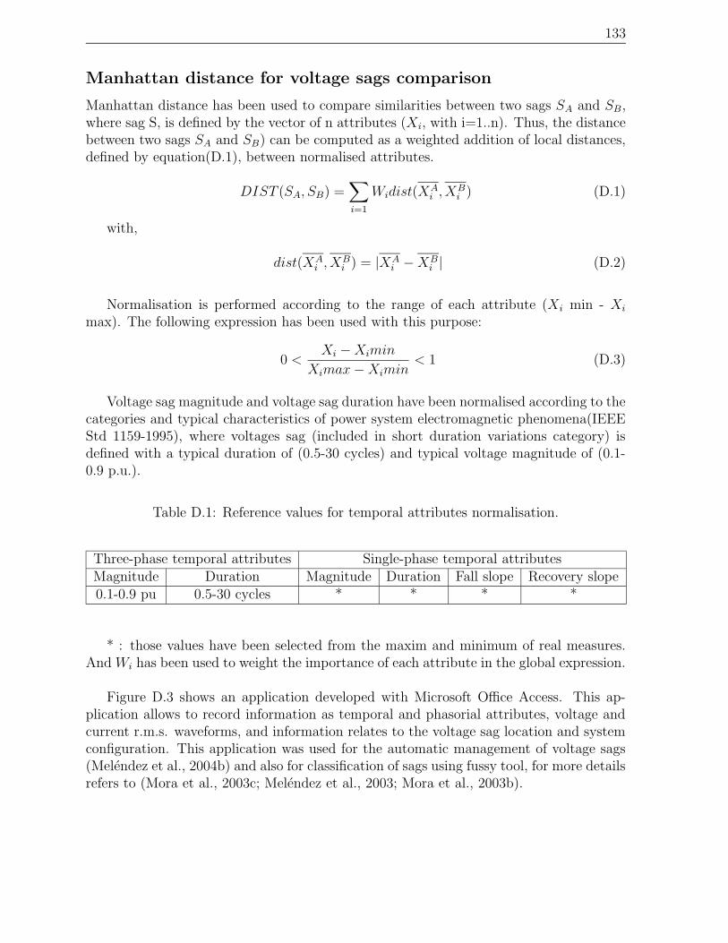
133
Manhattan distance for voltage sags comparison
Manhattan distance has been used to compare similarities between two sags SA and SB,where sag S, is defined by the vector of n attributes (Xi, with i=1..n). Thus, the distancebetween two sags SA and SB) can be computed as a weighted addition of local distances,defined by equation(D.1), between normalised attributes.
DIST (SA, SB) =∑
i=1
Widist(XAi , X
Bi ) (D.1)
with,
dist(XAi , X
Bi ) = |XA
i −XBi | (D.2)
Normalisation is performed according to the range of each attribute (Xi min - Xi
max). The following expression has been used with this purpose:
0 <Xi −Ximin
Ximax−Ximin< 1 (D.3)
Voltage sag magnitude and voltage sag duration have been normalised according to thecategories and typical characteristics of power system electromagnetic phenomena(IEEEStd 1159-1995), where voltages sag (included in short duration variations category) isdefined with a typical duration of (0.5-30 cycles) and typical voltage magnitude of (0.1-0.9 p.u.).
Table D.1: Reference values for temporal attributes normalisation.
Three-phase temporal attributes Single-phase temporal attributesMagnitude Duration Magnitude Duration Fall slope Recovery slope0.1-0.9 pu 0.5-30 cycles * * * *
* : those values have been selected from the maxim and minimum of real measures.And Wi has been used to weight the importance of each attribute in the global expression.
Figure D.3 shows an application developed with Microsoft Office Access. This ap-plication allows to record information as temporal and phasorial attributes, voltage andcurrent r.m.s. waveforms, and information relates to the voltage sag location and systemconfiguration. This application was used for the automatic management of voltage sags(Melendez et al., 2004b) and also for classification of sags using fussy tool, for more detailsrefers to (Mora et al., 2003c; Melendez et al., 2003; Mora et al., 2003b).

134 D. Temporal attributes of the voltage sags
Figure D.3: Developed Tool for voltage sags registration

Bibliography
Aamodt, A. and Plaza, E. (1994). Case-based reasoning: Foundational issues, method-ological variations, and system approaches. Artificial Intelligence Communications, IOSPress, 1:39–59.
Allemang, D. (1994). Combining case-based reasoning and task-specific architectures.IEEE Expert: Intelligent Systems and Their Applications, 9(5):24–34.
Armengol, J. (1999). Applications of the modal interval analysis to the simulation ofthe behaviour of dynamic systems with uncertain parameters. PhD thesis, University ofGirona.
Basseville, M. (1988). Detecting changes in signals and systems - a survey. Automatica,24(3):309–326.
Basseville, M. and Nikiforov, I. (1993). Detection of Abrupt Changes : Theory andApplication. Prentice Hall, New York.
Beard, R. V. (1971). Failure accommodation in linear systems through reorganization.Man Vehicle Lab Rep. MVT-7-1, Mass.Inst. Techno.
Berndt, J. and Clifford, D. (1994). Using dynamic time warping to find patterns in timeseries. pages 229–248. AAAI-94 Workshop on Knowledge Discovery in Database.
Blanke, M. (2005). Fault tolerant sensor fusion with an application to ship navigation.Prgaue, Czech Republic. 16th International Federation of Automatic Control WorldCongress IFAC’05.
Blanke, M., Kinnaert, M., Lunze, J., and M.Staroswiecki (2003). Diagnosis and Fault-Tolerant Control. Springer Verlag, Germany.
Bollen, M. H. (2000). Understanding Power Quality problems. IEEE Press series onpower engineering, New York.
Bonarini, A. and Bontempi, G. (1994). A qualitative simulation approach for fuzzydynamical models. ACM Transactions on Modeling and Computer Simulation, 4(4):258–313.
Brodsky, B. E. and Darkhovsky, B. S. (2000). Non-parametric Statistical Diagnosis.Problems and Methods. Kluwer Academic Publishers, ISBN 0-7923-8411-3.
135

136 BIBLIOGRAPHY
Calado, J. and Sa da Costa, J. (1999). On line fault detection and diagnosis based on acoupled system. European Control Conference.
Cassar, J. and Staroswiecki, M. (1997). A structural approach for the design or failuredetection and identification systems. pages 329–334, Belfort, France. IFAC/IFIP/IMACSConference on Control of Industrial Processes.
Chen, J. and Liao, C. M. (2002). Dynamic process fault monitoring based on neuralnetwork and PCA. Journal of Process Control, 12(2):277–289.
Chen, J. and Patton, R. J. (1999). Robust Model-based Fault Diagnosis for DynamicSystems. Kluwer Academic Publishers.
Chiang, L. H. and Braatz, R. D. (2003). Process monitoring using causal MAP andmultivariate statistics: fault detection and identification. Chemometrics and IntelligentLaboratory Systems, (65):159–178.
Chittaro, L., Guida, G., Tasso, C., and Toppano, E. (1993). Functional and teleologicalknowledge in the multimodeling approach for reasoning. IEEE Transactions on systems,man and cybernetics, 23(6):1718–1751.
Chouaib, B. (2004). Data Reconciliation as a Framework for Chemical Processes Opti-mization and Control. PhD thesis, Department of Chemical Engineering, PolytechnicalUniversity of Catalunya, Spain.
Chow, E. Y. and Willsky, A. S. (1984). Analytical redundancy and the design of robustfailure detection systems. IEEE Transactions on Automatic Control, AC-29:603–614.
Colomer, J. (1998). Representacio qualitativa asıncrona de senyals per a la supervisiode sistemes dinamics. PhD thesis, University of Girona, Thesis dissertation.
Colomer, J., Melendez, J., and Gamero, F. I. (2002). Pattern recognition based onepisodes and dtw. application to diagnosis of a level control system. Catalunya, Spain.6th International Workshop on Qualitative Reasoning.
Control-Eengineering-Practice (1997). Special volume on supervision, fault detection,and diagnosis of thecnical systems. Control Engineering Practice, 5(5).
Cordier, M., Dague, P., Levy, F., Montmain, J., Staroswiecki, M., and Trave-Massuye,L. (2004). Conflicts vesus analytical redundancy relations: A comparative analysis ofthe model based diagnosis approach from the artificial intelligence and automatic controlperspectives. IEEE Trans. on Syst, Man and Cyber- Part B:Cybernetics, 34(5):2163–2177.
Dague, P. (1995). Qualitative reasoning: a survey of techniques and applications.AICOM, (8).
De Kleer, J., Mackworth, A., and Reiter, R. (1992). Characterizing diagnoses andsystems. Artif. Intell., 56(2-3):197–222.

BIBLIOGRAPHY 137
De Kleer, J. and Williams, B. (1987). Diagnosing multiple faults. Artificial Intelligence,32(1):97–130.
De la Fuente, M. and Represa, C. (1997). A comparative study of neural networks basedapproach for fault detection. IFAC Safeprocess 1997.
Delmaire, G., Cassar, J. P., and Staroswiecki, M. (1994a). Comparison of identificationand parity space approaches for failure detection in single input single output systems.Proceedings of the Third IEEE Conference on Control Applications, 2:865 – 870.
Delmaire, G., Cassar, J. P., and Staroswiecki, M. (1994b). Identification and parity spacetechniques for failure detection in siso systems including modelling errors. Proceedingsof the 33rd IEEE Conference on Decision and Control, 3:2279 – 228.
Ding, S. X., Ding, E. L., and Jeinsch, T. (2002). A new optimization approach to thedesign of fault detection filters. In Proc. IFAC SAFEPROCESS 2000, pages 250–255,Budapest, Hungary,. SAFEPROCESS2000.
Ding, S. X., Jeinsch, T., Frank, P., and Ding, E. L. (2000). A unified approach tothe optimization of fault detection systems. Int. J. Adaptive Contr. Signal Processing,14(7):725–745.
Ding, S. X. and Zhang, P. (2005). Observer-based monitoring of distributed networkedcontrol systems. Ajaccion, France. 1st Workshop on Networked Control Systems andFault Tolerant Control.
Ding, X. and Jeinsch, T. (1999). An approach to analysis and design of observer andparity relation based fdi systems. 14th IFAC World Congress.
Dong, Y., Qing-Long, H., and Chen, P. (2004). State feedback controller design ofnetworked control systems. IEEE Transactions on Circuits and Systems II: Analog andDigital Signal Processing, 51, Issue:640–644.
El-Farra, N. H., Gani, A., and D.Christofides., P. (2005). Fault-tolerant control of processsystems using communication networks. AIChE Journal, 51, No. 6:1665–1682.
Fang, H., Ye, H., and Zhong, M. (2006). Fault diagnosis of networked control systems.China. IFAC Symposium on Fault Detection, Supervision and Safety of Technical Pro-cesses.
Fang, H., Ye, H., and Zhong, M. (2007). Fault diagnosis of networked control systems.Annual Reviews in Control, 31:55–68.
Frank, P. and Ding, X. (1997). Survey of robust residaul generation and evaluationmethods in observer-based fault detection systems. Journal of Process Control, 7(6):403–424.
Frank, P. M. (1990). Fault diagnosis in dynamic systems using analytical and knowledge-based redundancy - a survey and some results. Automatica, 26:459–474.

138 BIBLIOGRAPHY
Frank, P. M. (1996). Analytical and qualitative model-based fault diagnosis - a surveyand some new results. European Journal of Control, 2:6–28.
Gamero, F. I., Llanos, D., Colomer, J., and Melendez, J. (2004). Residual computationand evaluation using dynamic time warping. Genoa, Italy. IMACA.
Gertler, J. (1995). Diagnosing parametric faults-from identification to parity relations.pages 1615–1620, Seattle, WA. American Control Conference.
Gertler, J. (1998). Fault Detection and Diagnosis in Engineering Systems. MarcelDekker, New York.
Gertler, J. (2000). All linear mehtods are equal and extendible to nonlinearities. pages52–63, Budapest, Hungary. IFAC Sefeprocess.
Gertler, J., Costin, M., Fang, X., Kowalczuk, Z., Kunwer, M., and Monajemy, R. (1995).Model based diagnosis for automotive engines-algorithm development and testing on aproduction vehicle. IEEE Transactions on Control Systems Technologies, 3:61–69.
Gertler, J., Fang, X., and Luo, Q. (1990). Detection and diagnosis of plant failures: theorthogonal parity equation approach. Control and Dynamic Systems, 37:159–216.
Gertler, J. and Singer, D. (1990). A new structural framework for parity equation-basedfaiulure detection and isolation. Automatica, 26:381–388.
Gertler, J. J. (1991). Analytical redundancy methods in fault detection and isolation.pages 9–21. IFAC Symposium Safeprocess.
Goldberg, D. E. (1989). Genetic Algorithms in Search, Optimization, and MachineLearning. Addison-Wesley, USA.
Grainger, J. J. and Stevenson, W. D. (1998). Analisis de Sistemas de Potencia. Mexic.
Grinstead, C. M. and Snell, J. L. (1997). Introduction to Probability. 2nd edition.
Hamelin, F., Sauter, D., and Aubrun, M. (1994). Fault diagnosis in systems usingdirectional residuals. pages 3040– 3045. 33rd IEEE Conference on Decision and Control.
Hamscher, W., Console, L., and de Kleer, J. (1992). Readings in model based diagnosis.
Hu, S. and Zhu, Q. (2003). Stochastic optimal control and analysis of stability of net-worked control systems with long delay. Automatica, (39):1877–1884.
Iserman, R. (1997). Supervision, fault detection and fault-diagnosis methods-an intro-duction,. Control Engineering Practice, 5(5):639–652.
Isermann, R. (1984). Process fault detection based on modeling and estimation methods.Automatica, 20:387–404.
Isermann, R. and Balle, P. (1997). Trends in the application of model-based fault detec-tion and diagnosis of technical process. Control Engineering Practice, 5(5):709–719.
BIBLIOGRAPHY 139
Jalote, P. (1994). Fault Detection and Diagnosis in Engineering Systems. Prentice Hall,ISBN: 0133013677.
Jiang, B., Staroswiecki, M., and Cocquempot, V. (2002a). Fault identification for a classof timedelay systems. In Proc. Amer. Contr. Conf., pages 8–10, Anchorage, USA,. Amer.Contr. Conf.
Jiang, B., Staroswiecki, M., and Cocquempot, V. (2002b). h∞ fault detection filter fora class of discrete-time systems with multiple time delays. In Proc. 15th IFAC WorldCongress, Barcelona, Spain. 15th IFAC World Congress.
Jiang, B., Staroswiecki, M., and Cocquempot, V. (2003). h∞ fault detection filter designfor linear discrete-time systems with multiple time delays. Int. J. of Systems Science,34(5):365–373.
Jiang, C. and Zhou, D. H. (2005). Fault detection and identification for uncertain lineartime-delay systems. Computers & Chemical Engineering, (30):228–242.
Johannessen, S. (2004). Time synchronization in a local area network. IEEE ControlSystems Magazine, 24, Issue:61–69.
Kano, M., Hasebe, S., Hashimoto, I., and Ohno, H. (2001). A new multivariate statisticalprocess monitoring method using principal component analysis. Computers and ChemicalEngineering, 27(7-8):1103–1113.
Kassidas, A., MacGregor, J. F., and Taylor, P. A. (1998a). Synchronisation of batchtrajectories uring dynamic time warping. AIChEJ, 44(4):864–875.
Kassidas, A., Taylor, P. A., and MacGregor, J. F. (1998b). Off-line diagnosis of deter-ministic faults in continuous dynamic multivariable processes using speech recognitionmethods. J. Process Control, 8(5-6):381–393.
Keogh, E. and Pazzani, M. (2001). Derivative dynamic time warping. Chicago, USA. InProc. of the First Intl. SIAM Intl. Conf. on Data Mining.
Krzanowski, W. J. (1979). Between-group comparison of principle components. J. Am.Stat. Assoc., 74(367):703–707.
Kuipers, B. (1994). Qualitative reasoning-modelling and simulation with incompleteknowledge. MIT Press.
Kuipers, B. (2001). Qualitative simulation. In Robert A. Meyers, E.-i.-C., editor, Ency-clopedia of Physical Science and Technology, Third Edition, pages 287–300.
Kuipers, B. J. (1993). Reasoning with qualitative models. Artificial Intelligence, 59:125–132.
Langseth, H., A., A., and M, W. O. (1999). Learning retrieval knowledge from data. InAnand, A. and Aha, editors, IJCAI’99 Workshop ML-5: Automating the constructionof Case-Based Reasoners, pages 77–82.

140 BIBLIOGRAPHY
Lee, D., Allan, J., Thompson, H. A., and Bennett, S. (2001). Pid control for distributedsystem with a smart actuator. Control Engineering Practice, 9 (11):1235–1244.
Li, Y., Wen, C. L., Xie, Z., and Xu, X. H. (2004). Synchronisation of batch trajec-tory based on multi-scale dynamic time warping. pages 2403–2408. 2th InternationalConference on Machine Learning and Cybernetics (ICMLC 2003).
Li, Z. and Fang, H. (2006). A novel controller design and evaluation for networked controlsystems with time-variant delays. Journal of the Franklin Institute, 342(2):164–167.
Lian, F., Moyne, J., and Tilbury, D. (2003). Modelling and optimal controller design ofnetworked control systems with time delays. International Journal of Control, 76(6):591–606.
Llanos, D., Colomer, J., Melendez, J., and Staroswiecki, M. (2005). Influence of networkdelays in residual computation. Prague, Czech Republic. 16th IFAC World Congress.
Llanos, D., Cuberos, F. J., Melendez, J., Gamero, F. I., Colomer, J., and Ortega, J. A.(2003a). Recognition of system behaviours based on temporal series similarity. Com-putacion y Sistemas, 7(1):1–16.
Llanos, D., Gamero, F. I., Colomer, J., and Melendez, J. (2004a). Residual computationusing dynamic time warping. Seville, Spain. World Automation Congress.
Llanos, D., Melendez, J., and Colomer, J. (2004b). Fault diagnosis of dynamic sys-tems reusing cases. In AVR 2004 Jornada de Recerca en Automatica, Visio i Robotica,Barcelona.
Llanos, D., Melendez, J., Colomer, J., Mora, J., Corbella, J., and Sanchez, J. (2003b).Abstraction of significant temporal features of voltage sags recorded in a 25kv substation.page 85, Vigo, Spain. ICREPQ’03 International Conference on Renewable Energy andPower Quality.
Llanos, D., Staroswiecki, M., Colomer, J., and Melendez, J. (2006). Minimising falsealarms caused by communication delays in networked systems. IFAC Safeprocess 2006.
Llanos, D., Staroswiecki, M., Colomer, J., and Melendez, J. (2007). Transmission delaysin residual computation. IET Control Theory & Applications, 1(5):1471–1476.
Lopez, R. and Plaza, E. (1997). Case-based reasoning: An overview. AI CommunicationsIOS Press, 10(1):21–29.
Luck, R. and Ray, A. (1990). An observer-based compensator for distributed delay.Automatica, 26(5):903–908.
Ma, C. and Fang, H. (2005). Stability of networked control systems with multi-stepdelays based on time-division algorithm. Journal of Control Theory and Applications,3(4):404–408.
Main, J., Dillon, T. S., and Shiu, S. C. K. (2001). Soft computing in case based reasoning,chapter A tutorial on case based reasoning, pages 1–28. Springer-Verlag, London, UK.
BIBLIOGRAPHY 141
Maquin, D. and Ragot, J. (1991). Comparison of gross errors detection methods onprocess data. pages 2254–2261, Brigthon, England. 30th Conference on Decision andControl.
Matveev, A. S. and Savkin, A. V. (2003). The problem of state estimation via asyn-chronous communication channels with irregular transmission times. IEEE Trans. onAutomatic Control, 48(4):670–676.
Melendez, J., Macaya, D., Colomer, J., and Llanos, D. (2004a). Symptom based rep-resentation for dynamic systems diagnosis.application to electrical power distribution.Madrid, Spain. 7th European Conference on Case-Based Reasoning (ECCBR2004) -2nd Workshop on applying case-based re.
Melendez, J., Macaya, D., Llanos, D., Cobos, J., Sanchez, J., and Castro, M. (2004b).Automatic management of voltage sags recorded in a 25kv substation. Barcelona, Spain.ICREPQ’04 International Conference on Renewable Energy and Power Quality.
Melendez, J., Mora, J., Llanos, D., Ruiz, M., Colomer, J., and Corbella, J. S. . J. (2003).Classification of short duration faults (voltage sags) in transmission and distributionpower systems. University of Cambridge (UK). ECC’03, European Control Conference.
Mendes, M., Calado, J., and Sa da Costa, J. (2006). Fault diagnosis system based inagents. pages 427–432. IFAC Safeprocess 2006.
Mendoca, L., Sousa, J., and Sa da Costa, J. (2008). An architecture for fault detectionand isolation based on fuzzy methods. Expert Systems with Applications, 2008.
Montestruque, L. A. and Antsaklis, P. J. (2003). On the model-based control of net-worked systems. Automatica, 39:1837–1843.
Montestruque, L. A. and Antsaklis, P. J. (2004). Stability of model-based networkedcontrol systems withtime-varying transmission times. IEEE Transactions on AutomaticControl, 49, Issue:1562–1572.
Mora, J., Llanos, D., Melendez, J., Colomer, J., and Sanchez, J. (2003a). Classification ofsags measured in a distribution substation based on qualitative and temporal attributes.Barcelona. CIRED, 17th International Conference on Electricity Distribution.
Mora, J., Llanos, D., Melendez, J., Colomer, J., Sanchez, J., and Cobella, J. (2003b).Clasificacion de huecos de tension con base en descriptores cualitativos y temporales.Jornada Nacional de Enegıa Electrica - CIRED.
Mora, J., Melendez, J., Llanos, D., Colomer, J., Corbella, J., and Sanchez, J. (2003c).Classification of sags measured in a distribution substation using a fuzzy tool. page 89,Vigo, Spain. ICREPQ’03 International Conference on Renewable Energy and PowerQuality.
Neidiga, J. and Lunze, J. (2005). Decentralised diagnosis of automata networks. Pro-ceedings of the 16ht IFAC World Congress.

142 BIBLIOGRAPHY
Nikiforov, I., Staroswiecki, M., and Vozel, B. (1996). Duality of analytical redundancyand statistical approach in faultdiagnosis. Proceedings of the 13th IFAC World Congress.
Nilsson, J. (1998). Real-Time Control Systems with Delays. Doctoral dissertation, LundInstitute of Technology, Lund, Sweden.
Nilsson, J., Bernhardsson, B., and Wittenmark, B. (1988). Stochastic analysis andcontrol of real-time systems with random time delays. Automatica, 34:57–64.
Nomikos, P. and MacGregor, J. F. (1994). Monitoring batch process using multiwayprinciple component analysis. AIChEJ, 40(8):1361–1375.
Ogata, K. (1997). Modern Control Engineering. Prentice Hall, Englewood Cliffs, NJ,3rd edition.
Patankar, R. (2004). A model for fault-tolerant networked control system usingttp/ccommunication. IEEE Transactions on VehicularTechnology, 53, Issue:1461–1467.
Patton, R. J. and Chen, J. (1991). A review of parity space approaches to fault diagnosis.Baden-Baden. Ifac Safeprocess Symposium.
Puig, V., Quevedo, J., Escobet, T., and De las Heras, S. (2002). Robust fault detectionapproaches using inteval models. Barcelona. IFAC World Congress.
Quinlan, J. R. (1986). Induction of decision trees. Mach. Learn., 1(1):81–106.
Rabiner, L. and Juang, B. (1993). Fundamentals of Speech Recognition. Prentice Hall.
Raich, A. and Cinar, A. (1997). Diagnosis of process disturbances by statistical distanceand angle measures. Comput. Chem. Eng., 21(6):661–673.
Reiter, R. (1987). A therory of diagnosis from first principles. Artificial Intelligence,32(1):57–96.
Reklaitis, G. V., Ravindran, A., and Ragsdell, K. M. (1983). Engineering Optimization.Methods and Applications. John Wiley and Sons, USA.
Sakoe, H. and Chiba, S. (1978). Dynamic programmning algorithm optimization for spo-ken word recognition. IEE Trans. acoustics, Speech and Signal Proc., ASSP-26(1):43..49.
Sankoff, D. and Kruskal, J. (1983). Time Warps, String Edits, and Macromolecules:The Theory and Practice of Sequence Comparison. Addison Wesley.
Sauter, D. and Boukhbza, T. (2006). Robustness against unknownnetworked induceddelays of observer based FDI. IFAC Safeprocess 2006, pp 331–336.
Sauter, D., Boukhbza, T. and Hamelin, F. (2006). Decentralized and autonomous designfor FDI/FTC of networked control systems. IFAC Safeprocess 2006, pp 163–168.
Sauter, D., Mary, N., Sirou, F., and Thieltgen, A. (1994). Fault diagnosis in systemsusing fuzzy logic. pages 883 – 888. Third IEEE Conference on Control Applications.

BIBLIOGRAPHY 143
Savkin, A. V. and Petersen, I. R. (2003). Set-valued state estimation via a limitedcapacity communication channel. IEEE Trans. on Automatic Control, 48(4):676–680.
Sa da Costa, J., Santos, B., and Mendes, M. (2007). Multi-agent toolbox for faulttolerant networked control systems design. Nancy, France. 3rd International Workshopon Networked Control Systems : Tolerant to Faults.
Shanbin, L., Sauter, D., and Aubrun, C. (2006). Robust fault isolation filter designfor networked control systems. pages 681 – 688, Czech Republic. IEEE Conference onEmerging Technologies and Factory Automation. ETFA ’06.
Silverman, H. F. and Morgan, D. P. (1990). The application of dynamic programmingto connected speech recognition. IEEE ASSP Magazine, 7:6–25.
Simoudis, E. (1992). Using case-based retrieval for customer technical support. IEEEExpert: Intelligent Systems and Their Applications, 7(5):7–12.
Singhal, A. and Seborg, D. E. (2002). Pattern matching in historical batch data usingpca. IEEE Control Syst., 22(5):53–63.
Srinivasan, R., Wang, C., Ho, W., and Lim, K. (2004). Dynamic pca based methodologyfor clustering process states in agile chemical plants. Ind. Eng. Chem. Res, 43(9):2123–2139.
Staroswiecki, M. (2005). Intelligent sensors : A functional view. IEEE Tr. on IndustrialInformatics, 1(4).
Staroswiecki, M., Cassar, J. P., and Declerck, P. (2000). A structural framework for thedesign of fdi systems in large scale industrial plants. In Clark, R. N., Patton, R. J., andFrank, P. M., editors, Issues of Fault Diagnosys for Dynamic Systems. Springer-Verlag.
Staroswiecki, M. and Comtet-Varga, G. (2001). Analytic redundancy relations for faultdetection and isolation inalgebraic dynamic systems. Automatica, 37, Issue(5):687–699.
Tipsuwan, Y. and Chow, M. Y. (2003). Control methodologies in networked controlsystems. Control Engineering Practice, 11:1099–1111.
Trave-Massuyes, L. and Dague, P. (2003). Modeles et raisonnements qualitatifs.
Trave-Massuyes, L., Escobet, T., Pons, R., and Tornil, S. (2001). The caen diagnosissystem and its automatic modelling method. Computacion y sistemas, 5(2):128–143.
Trevelyan, J. (2004). Industrial process communications and software. Technical report,Mechatronics Design 310, http://www.mech. uwa.edu.au/mechatronics/site-index.html.
Trinh, H. and Aldeen, M. (1997). A memoryless state observer for discrete time-delaysystems. IEEE Trans. on Automatic and Control, 11(42):1572–1577.
Venkatasubramanian, V., Rengaswamy, R., Yin, K., and Kavuri, S. H. (2003). A reviewof process fault detection and diagnosis parts: I, ii, and iii. Computer and ChemicalEnegineering, 27:293–346.

144 BIBLIOGRAPHY
Villegas, T. and De la Fuente, M. (2006). Fault diagnosis using an observers bank of dy-namical neural networks. St. Louis, EEUU. Neural Networks in Engineering ANNIE’06.
Vitturi, S. (2000). Some features of two feildbuses of the iec 61158. Computer Standardsand Interfaces, 22:203–215.
Walsh, G. C., Beldiman, O., and Bushnell, . G. (2002). Error enconding algorithms fornetworked control systems. Automatica, 38:264–267.
Walsh, G. C. and Hong, Y. (2001). Scheduling of networked control systems. IEEEControl System Magazine, pages 57–65.
Wang, Z., Daniel, W. C., and Liu, X. (2003). Variance-constrained filtering for uncertainstochastic systems with missing measurements. IEEE Trans. on Automatic Control,48(7):1254–1258.
Webb, A. R. (2002). Statsitical Pattern Recognition. John Wiley and Sons Ltd., 2ndedition.
Wilke, W. and Bergmann, R. (1998). Techniques and knowledge used for adaptationduring case-based problem solving. In IEA/AIE ’98: Proceedings of the 11th Interna-tional Conference on Industrial and Engineering Applications of Artificial In telligenceand Expert System, pages 497–506, London, UK.
Willsky, A. S. (1976). A survey of design methods for failure detection in dynamicsystems,. Automatica, 12:601–611.
Xie, L., Ji, Z., Pan, T., and Fang, H. (2005). Fault detection for networked con-trol systems with asynchronous measurements delays. Jounal of System Simulation,11(17):2717–2720.
Yang, H. L. and Saif, M. (1998). Observer design and fault diagnosis for state-retardeddynamical systems. Automatica, 34(2):217–227.
Ye, H., He, R., Liu, H., and G.Wang (2006). A new approach for fault detection ofnetworked control systems. pages 654–659, Australia. IFAC 14th Symposium on SystemIdentification.
Ye, H., Wang, G., and Ding, S. (2004). A new parity espace approach for fault detectionbased on stationary wavelet transform. IEEE Trans. on Automatic Control, 2(49):281–287.
Ye, H., Zhang, P., Ding, S., and Wang, G. (2000). A time.frequency domain faultdetection approach based on parity relation and wavelet transform. pages 4156–4161,Australia. 39th IEEE Conference on Decision and Control.
Yi, B. K., Jagadish, H., and Faloustsos, C. (1998). Efficient retrieval of similar timesequences under time warping. pages 23–27.

BIBLIOGRAPHY 145
Z. Bak, M., Larsen, T. D., Norgaard, M., Andersen, N. A., Puolsen, N. K., and Ravn,O. (1998). Location estimation using delayed measurements. pages 180–185, Coimbra.5th International Workshop on Advanced Motion Control AMC98.
Zhang, P. and Ding, S. X. (2007). On Monotonicity of a class of optimal fault detectionperformance versus sampling period. pages 2596–2601, New Orleans, LA, USA,. 46thIEEE Conference on Decision and Control.
Zhang, P., Ding, S. X., Frank, P. M., and Sader, M. (2004). Fault detection of networkedcontrol systems with missing measurements. pages 1258–1263, Melbourne, Australia. 5thAsian Control Conference.
Zhang, P., Ye, H., Ding, S. X., Wang, G., and Zhou, D. (2006). On the relationshipbetween parity space and h2 approaches to fault detection. Systems & Control Letters,2(55):91–100.
Zhang, W., Branicky, M. S., and Phillips, S. M. (2001). Stability of networked controlsystems. IEEE Control Systems Magazine, pages 84–99.
Zheng, Y., Fang, H., and Wang, H. (2004). Kalman filter based fault detection ofnetworked control system. pages 1330–1333, China. 4th World Congress on IntelligentControl and Automation.
Zheng, Y., Fang, H., Wang, H., and Li, L. (2003a). Observer-based fdi design of net-worked control system with output transfer delay. Control Theory and Applications,5(20):653–663.
Zheng, Y., Fang, H., Wang, H., and Xie, L. (2003b). Fault detection approach for net-worked control system based on a memoryless reduced-order observer. ACTA AutomaticaSINICA, 4(29):559–566.
Zheng, Y., Hua, X., Fang, H., and Wang, H. (2005). Research on observed-based faultdiagnosis of networked control system. Systems Engineering and Electronics, 6(27):1069–1072.
Zhivoglydov, P. V. and Middleton, R. H. (2003). Networked control design for linearsystems. Automatica, pages 743–750.
Zhong, M., Ye, H., Wang, G., and Zhou, D. (2005). Fault detection filter for linear timedelay systems. Nonlinear Dynamics and Systems Theory, 5(3):273–284.
Zhong, M. S., Ding, S. X., and Lam, J. (2004). An optimization approach to faultdetection observer design for neutral delay systems. Dynamics of Continuous, Discreteand Impulsive Systems (B), 11(6):701–721.