time-integration schemes for the finite …cermics.enpc.fr/~ern/pdfs/11_dep_sisc.pdf ·...

SIAM J. SCI. COMPUT. c© 2011 Society for Industrial and Applied MathematicsVol. 33, No. 1, pp. 223–249

TIME-INTEGRATION SCHEMES FOR THE FINITE ELEMENTDYNAMIC SIGNORINI PROBLEM∗

DAVID DOYEN†, ALEXANDRE ERN‡ , AND SERGE PIPERNO‡

Abstract. A large variety of discretizations have been proposed in the literature for the nu-merical solution of the dynamic Signorini problem. We classify the different discretizations intofour groups. The first three groups correspond to different ways of enforcing the contact condition:exact enforcement, enforcement with penalty, and enforcement with contact condition in velocity.The fourth approach is based on a modification of the mass matrix. Numerical simulations on twoone-dimensional benchmark problems with analytical solutions illustrate the properties of represen-tative methods within each class, focusing first on spurious oscillations triggered by contact and thenon energy behavior after multiple impacts. Selected schemes are also tested on a two-dimensionalbenchmark.

Key words. elastodynamics, frictionless unilateral contact, time-integration schemes, finiteelements, modified mass method

AMS subject classifications. 65M20, 65M60, 74H15, 74M15, 74S05

DOI. 10.1137/100791440

1. Introduction. The design of robust and efficient numerical methods for dy-namic contact problems has motivated a large amount of work over the last twodecades and remains challenging. Here, we focus on the dynamic Signorini problem,which models the infinitesimal deformations of a solid body that can come into con-tact with a rigid obstacle. This problem is the simplest dynamic contact problem, butalso the first step toward more complex situations such as multibody problems, largedeformation problems, contact with friction, etc. For an overview of the differentcontact problems, we refer the reader to [21, 25, 38].

In structural dynamics, the usual space-time discretization combines finite ele-ments in space and a time-stepping scheme. In this framework, the discretization ofthe dynamic Signorini problem involves mainly three choices: (i) the finite elementspace, (ii) the enforcement of the contact condition, (iii) the time-stepping scheme.The combination of these three ingredients presents some difficulties. For instance, itis well known that the combination of an exact enforcement of the contact conditionand an implicit Newmark scheme yields spurious oscillations as well as poor energybehavior, that is, sizeable deviations from the exact value. Moreover, the combinationof an exact enforcement and an explicit scheme is not straightforward, whereas theuse of a penalty contact condition tightens the stability condition of explicit schemes.Consequently, various alternative discretizations have been designed for the dynamicSignorini problem. The aim of this work is to classify the different discretizations andto numerically illustrate their main properties.

We classify the discretizations into four groups. The first three groups correspondto different ways of enforcing the contact condition: exact enforcement [6, 8, 18, 27,

∗Submitted to the journal’s Computational Methods in Science and Engineering section April 7,2010; accepted for publication (in revised form) November 2, 2010; published electronically February3, 2011.

http://www.siam.org/journals/sisc/33-1/79144.html†Electricite de France (EDF R&D), 1 avenue du General de Gaulle, 92141 Clamart Cedex, France

([email protected]).‡Universite Paris-Est, CERMICS, Ecole des Ponts, 77455 Marne la Vallee Cedex 2, France

([email protected], [email protected]).

223

224 DAVID DOYEN, ALEXANDRE ERN, AND SERGE PIPERNO

31, 32, 36, 37], enforcement with penalty [1, 3, 15], and enforcement with contactcondition in velocity [2, 3, 26]. The fourth approach is based on a modification ofthe mass matrix [14, 20]; it can be seen as an alternative choice of the finite elementspace. These four classes yield different space semidiscrete problems, which in turncan be discretized in time using various time-stepping schemes, either implicit orsemiexplicit. We select representative discretizations within each class and examinetheir main properties: presence of spurious oscillations, energy behavior after multipleimpacts, and stability in the case of explicit schemes. By energy conservation we meanthat the variation of the energy is equal to the work of the external forces (the contactforces should not work). To illustrate these properties, numerical simulations on twoone-dimensional (1D) benchmarks have been performed. The first benchmark, theimpact of an elastic bar on a rigid surface, is well known and allows one to detectspurious oscillations. The second, for which we derive the exact solution, deals withthe bounces of an elastic bar and is geared toward energy behavior, insofar as multipleimpacts occur; it is, to our knowledge, a new benchmark. Additionally, some of theschemes are tested on a two-dimensional (2D) benchmark (without analytical solution)associated with the impact and multiple bounces of a disk on a rigid surface. Someof the presented Newmark-based schemes are also compared in three dimensions in[23]. The mathematical analysis of the different methods is beyond the scope of thisarticle, but we mention, whenever they exist, the theoretical results (well-posednessof the discrete problems and convergence of the discrete solutions). Dynamic contactproblems yield shock waves, and spurious oscillations appear near the shock in thenumerical solutions, owing to the so-called Gibbs phenomenon (see, e.g., [13] andreferences therein). These oscillations can be eliminated using dissipative schemes (or,equivalently, by filtering). This issue, being important but not specific to dynamiccontact problems, is not further addressed here (see also Remark 4.4).

The material is organized as follows. We formulate the dynamic Signorini prob-lem in the continuous setting (section 2.1), and we introduce the main ingredients forits approximation (sections 2.2 and 2.3). We present the two 1D benchmark problemswith their analytical solutions (section 3). We describe the four classes of discretiza-tions together with numerical results in one dimension: exact enforcement of thecontact condition (section 4), enforcement with penalty contact condition (section 5),enforcement with contact condition in velocity (section 6), and modification of themass matrix (section 7). Finally, we present numerical results on the 2D benchmarkfor selected schemes (section 8) and draw some conclusions (section 9).

2. The dynamic Signorini problem.

2.1. Governing equations. We consider the infinitesimal deformations of abody occupying a reference domain Ω ⊂ R

d (d ∈ {1, 2, 3}) during a time interval [0, T ].The tensor of elasticity is denoted by A, and the mass density is denoted by ρ. Anexternal load f is applied to the body. Let u : (0, T )×Ω → R

d, ε(u) : (0, T )×Ω → Rd,d,

and σ(u) : (0, T )× Ω → Rd,d be the displacement field, the linearized strain tensor,

and the stress tensor, respectively. Denoting time-derivatives by dots, the momentumconservation equation reads

(2.1) ρu− div σ = f, σ = A : ε, ε =1

2(∇u+ T∇u) in Ω× (0, T ).

The boundary ∂Ω is partitioned into three disjoint open subsets, ΓD, ΓN , and Γc.Dirichlet and Neumann conditions are prescribed on ΓD and ΓN , respectively u = uD

on ΓD × (0, T ) and σ · n = fN on ΓN × (0, T ), where n denotes the outward unit

DISCRETIZATIONS FOR THE DYNAMIC SIGNORINI PROBLEM 225

normal to Ω. We set un := u|∂Ω · n and σn := n · σ|∂Ω · n, the normal displacementand the normal stress on ∂Ω, respectively. On Γc, a unilateral contact condition, alsocalled Signorini condition, is imposed:

(2.2) un ≤ 0, σn(u) ≤ 0, σn(u)un = 0 on Γc × (0, T ).

At the initial time, the displacement and velocity fields are prescribed. The aboveproblem is an evolution partial differential equation under unilateral constraints. Here,the equation is second-order in time, and the constraint holds on the displacement;this is not the most favorable case. The existence and uniqueness of a solution hasbeen proven only in one dimension, when the contact boundary is reduced to a point[28, 11]. In one dimension, it has also been proven that the variation of energy isequal to the work of the external forces; the contact force does not work [28, 11]. Inhigher dimensions, the existence of a solution is proven in the case of a viscoelasticmaterial, and, under certain assumptions, existence and uniqueness are proven for thewave equation [28, 11].

2.2. Basic time-integration schemes in linear elastodynamics. In thissection, we briefly recall some basic facts about time-integration schemes in linearelastodynamics; most of this material can be found in [17]. First, we discretize theproblem in space with a finite element method. To simplify the notation, we stilldenote by u the space semidiscrete displacement. The number of degrees of freedomis denoted by Nd. Let K, M , and F (t) be the stiffness matrix, the mass matrix, andthe column vector of the external forces, respectively. The space semidiscrete problemconsists of seeking u : [0, T ] → R

Nd such that, for all t ∈ [0, T ],

(2.3) Mu(t) +Ku(t) = F (t),

with the initial conditions u(0) = u0 and u(0) = v0. For solving such a system of or-dinary differential equations (ODEs), linear one-step schemes are the most frequentlyused. For simplicity, the interval [0, T ] is divided into equal subintervals of length Δt.We set tn = nΔt and denote by un, un, and un the approximations of u(tn), u(tn), andu(tn), respectively. We define the convex combination �n+ω := (1 − ω)�n + ω�n+1,where � stands for u, u, u or t, and ω ∈ [0, 1]. We use a slightly different definition for

the external load, namely, Fn+α := F (tn+α); for instance, Fn+ 12 = F (tn+

12 ) generally

differs from 12 (F

n + Fn+1). Moreover, at time tn, the energy of the system is givenby En := 1

2TunMun + 1

2TunKun. Now we can formulate some of the most common

time-stepping schemes in linear elastodynamics.Discretization 2.1 (Hilber–Hughes–Taylor (HHT)-Newmark). Seek un+1, un+1,

un+1 ∈ RNd such that

Mun+1 +Kun+1+α = Fn+1+α,(2.4)

un+1 = un +Δt un +Δt2

2un+2β,(2.5)

un+1 = un +Δt un+γ ,(2.6)

where α, β, γ are real parameters. The choice α = 0 yields Newmark schemes, whilethe choice α ∈ [−1/3, 0], β = 1/4(1− α)2, and γ = 1/2− α yields HHT schemes.


Discretization 2.2 (midpoint). Seek un+1, un+1, un+ 12 ∈ R

Nd such that

Mun+ 12 +Kun+ 1

2 = Fn+ 12 ,(2.7)

un+1 = un +Δt un+ 12 ,(2.8)

un+1 = un +Δt un+ 12 .(2.9)

Discretization 2.3 (central differences). Seek un+1 ∈ RNd such that

(2.10) M

(un+1 − 2un + un−1

Δt2

)+Kun = Fn.

HHT schemes are implicit, unconditionally stable, second-order accurate, anddissipative in the high frequencies. The amount of dissipation is controlled by theparameter α. Newmark schemes do not, in general, conserve the energy; such schemes

instead conserve the quadratic form Enβ,γ := En + Δt2

2

(β − 1

2γ)TunMun since there

holds [24]

En+1β,γ − En

β,γ = T

(1

2(Fn+1 + Fn) +

(γ − 1

2

)(Fn+1 − Fn)

)(un+1 − un)

−(γ − 1

2

)(T(un+1 − un)K(un+1 − un)

+

(β − 1

2γ

)T(un+1 − un)M(un+1 − un)

).

The quadratic form Enβ,γ coincides with the energy only if β = 1

2γ. For β �= 12γ, we

refer to Enβ,γ as a shifted energy; the sign of the difference between En

β,γ and En depends

only on the sign of (β− 12γ). The particular choice β = 1/4, γ = 1/2 yields an implicit,

unconditionally stable, and second-order accurate scheme. It is energy-conserving inthe sense that

En+1 − En = T

(Fn+1 + Fn

2

)(un+1 − un).

The midpoint scheme is implicit, unconditionally stable, and second-order accurate.It is energy-conserving in the sense that

En+1 − En = TFn+ 12 (un+1 − un).

The central difference scheme is explicit (lumping the mass matrix avoids solving anylinear system), conditionally stable, and second-order accurate. Here it is written asa two-step linear scheme involving only the displacement, but it can be formulatedas a one-step scheme. Actually, it is a Newmark scheme with parameters β = 0,γ = 1/2; the velocity and acceleration are then un = 1

2Δt (un+1 − un−1) and un =

1Δt2 (u

n+1 − 2un + un−1). The central difference scheme does not conserve the energyEn but the shifted energy En

0, 12in the sense that

En+10, 12

− En0, 12

= T

(Fn+1 + Fn

2

)(un+1 − un).

There exist also explicit schemes with high-frequency dissipation, such as the Chung–Hulbert or Tchamwa–Wielgosz schemes (see [30] and references therein).


2.3. Enforcing the contact condition. The enforcement of a contact con-dition in a finite element setting has been widely studied in the case of the staticSignorini problem [21]. We assume that the mesh is compatible with the partition ofthe boundary. Let Nc be the number of nodes lying on the contact boundary. Wedefine the linear normal trace operator on Γc, g : v �−→ −v|Γ · n, and the associatedmatrix G. Note that the dimension of G is Nc ×Nd. We denote by {Gi}1≤i≤Nc therows of the matrix G. Thus, Giu yields the value of the normal displacement at theith node of the contact boundary. With an exact enforcement, the static Signoriniproblem consists of seeking a displacement u ∈ R

Nd and a contact pressure r ∈ RNc

such that

Ku = F + TGr,(2.11)

Gu ≥ 0, r ≥ 0, TrGu = 0.(2.12)

Here the problem is formulated as a complementarity problem. Other formalisms canbe found in the literature, e.g., variational inequality, Lagrangian formulation, andformulation with subderivatives. If the matrix K is positive definite, problem (2.11)–(2.12) has a unique solution. For solving this problem, a large variety of methods havebeen developed [21, 38]: Uzawa algorithms, active set methods, semismooth Newtonmethods, the Lemke algorithm, the monotone multigrid method, etc.

Penalty formulations are another classical way of dealing with constrained prob-lems. We have to define a penalty function Rε : RNc → R

Nc . For instance, we canchoose Rε(v) = 1

ε (v)−, where (v)− denotes the negative part of v. The penalized

static Signorini problem consists now of seeking u ∈ RNd such that

(2.13) Ku = F + TGRε(Gu).

A third way of enforcing the contact condition, specific to the dynamic problem, isto replace the Signorini condition by an approximation involving the velocity insteadof the displacement [11, 29]. Assume that un = 0 at a certain time tc. Then, on ashort time interval afterwards, un ≈ (t− tc)un. This motivates the following contactcondition in velocity:

(2.14) un ≤ 0, σn(u) ≤ 0, σn(u)un = 0 on Γc.

It must be stressed that condition (2.14) is applicable only during contact phases.This condition is not applicable during noncontact phases because a positive normalvelocity is not allowed.

3. 1D benchmark problems. To compare the different methods, we test themon two 1D problems. Both problems can be formulated in the same setting. We con-sider an elastic bar dropped against a rigid ground. The bar is dropped, undeformed,from a height h0, with an initial velocity −v0, under a gravity acceleration g0 ≥ 0.The length of the bar is denoted by L, the Young modulus by E, and the density by ρ.

Let c0 :=√

Eρ denote the wave speed. The reference domain is Ω = [0, L]. In this

context, the governing equations presented in section 2.1 for the continuous problemtake the form

ρu− E∂2u

∂x2= −ρg0 in Ω× (0, T ),(3.1)

u(0, t) ≥ 0, r(t) ≥ 0, r(t)u(0, t) = 0 on (0, T ),(3.2)

∂u

∂x(L, t) = 0 on (0, T ), u(·, 0) = h0, u(·, 0) = −v0,(3.3)


��

��

��

��

��

��

t = 0 t1

−v0

−v0

v0

t2

v0−v0

00

0

Fig. 1. Impact of an elastic bar.

where u is the scalar-valued displacement of the bar and r the contact pressure equalto the normal stress −E ∂u

∂x at x = 0. Problem (3.1)–(3.3) has a unique solution, andthe variation of the energy is equal to the work of the gravity force [28],

(3.4)d

dt

(1

2

∫Ω

ρu2 +1

2

∫Ω

E

∣∣∣∣∂u∂x∣∣∣∣2)

=

∫Ω

−ρg0u ∀t ∈ [0, T ].

In the first problem, v0 > 0 and g0 = 0 so that there is a single impact. Thisbenchmark has been widely used in the literature (see, e.g., [38]). It enables us toexamine the possible spurious oscillations triggered by the numerical schemes. In thesecond problem, v0 = 0 and g0 > 0, so that the bar can make several bounces. Witha suitable choice of parameters, the motion of the bar is periodic in time, and wecan calculate the exact solution. This benchmark enables us to examine the timeevolution of energy after multiple impacts and is, to our knowledge, new.

3.1. Impact of an elastic bar. Let us describe the solution of the first problem(Figure 1). Before the impact, the bar is undeformed and has a uniform velocity −v0.The bar reaches the ground at time t1 := h0

v0. After the impact, the bar stays in

contact with the ground. A shock wave travels from the bottom of the bar to thetop. Above the shock wave, the velocity is −v0; below, the velocity is zero. Then, theshock wave travels from the top to the bottom. Above the shock wave, the velocity isv0; below, the velocity is still zero. As soon as the wave reaches the bottom, the bartakes off, undeformed, with a uniform velocity v0. The speed of the shock wave is c0.Thus, the wave takes a time τw := L

c0to travel along the bar, and the bar takes off at

time t2 := t1 + 2τw. The analytical solution can be easily expressed using travellingwave solutions. Defining the auxiliary function Hv(x, t) = −vmin(x/c0, τw−|t−τw|),the exact solution is

u(x, t) =

⎧⎪⎨⎪⎩h0 − v0t if t ≤ t1,

Hv0(x, t− t1) if t1 < t ≤ t2,

v0(t− t2) if t2 < t.

In particular, the displacement at the bottom of the bar and the contact pressure are

u(0, t) =

⎧⎪⎨⎪⎩h0 − v0t if t ≤ t1,

0 if t1 < t ≤ t2,

v0(t− t2) if t2 < t,

r(t) =

⎧⎪⎨⎪⎩0 if t ≤ t1,Ev0c0

if t1 < t ≤ t2,

0 if t2 < t.

These two quantities are represented in Figure 2 (with the parameters chosen insection 3.3).


-0.2

-0.1

0

0.1

0.2

0.3

0.4

0.4 0.5 0.6 0.7 0.8 0.9 1 1.1 1.2 1.3

disp

lace

men

t

time

exact solution-100

0

100

200

300

400

500

0.4 0.5 0.6 0.7 0.8 0.9 1 1.1 1.2 1.3

cont

act p

ress

ure

time

exact solution

Fig. 2. Impact of an elastic bar. Displacement at the bottom of the bar (left) and contactpressure (right).

��

��

��

��

��

��

t = 0 t1 t2 t3 t4

−vf vfvf −vf

v0

Fig. 3. Bounces of an elastic bar.

3.2. Bounces of an elastic bar. In the second problem (Figure 3), the bar

is dropped, undeformed, with a zero initial velocity. It takes a time τf :=√

2h0

g0to

reach the ground. At the impact, at time t1 := τf , the bar is undeformed and hasuniform velocity −vf , where vf :=

√2h0g0. After the impact, as in the previous

benchmark, the bar stays in contact with the ground during a time 2τw. Duringthis contact phase, the response of the bar is the superposition of a shock wavedue to velocity at the impact and a vibration due to the gravity, as reflected bythe series S1 and S2 below. When the bar takes off, at time t2 := t1 + 2τw, ithas a uniform velocity vf but it is compressed. (By symmetry, u(x, t2) = u(x) :=g0c20(x2−2Lx) is twice the static deformation with homogeneous Dirichlet and Neumann

conditions at x = 0 and x = L, respectively.) Consequently, during the flight phase,the response of the bar is the superposition of a rigid parabolic motion (due to thegravity and the velocity) and a vibration (due to the initial deformation). If wechoose τf = pτw for a positive integer p (for instance, τf = 3τw), we can ensurethat the bar reaches the ground with uniform velocity −vf and with displacementfield u. When we do this, the second impact occurs at time t3 := t2 +2τf = t2 +6τw.When the bar takes off again, at time t4 := t3 + 2τw, it is undeformed and has auniform velocity vf . The next flight phase is a rigid parabolic movement. Then thissequence of two contact phases and two flight phases repeats periodically. To computethe analytical solution, we use a decomposition on the eigenmodes in addition tothe travelling wave solutions. We set t4k+1 = 3τw + 16kτw, t4k+2 = t4k+1 + 2τw,t4k+3 = t4k+1+8τw, and t4k+4 = t4k+1+10τw. We also define the auxiliary functionsP (x, t) = h0 − 1

2g0(t − τf )2, S1(x, t) =

∑∞n=1 an(1 − cos(c0νnt)) sin(νnx), S2(x, t) =

− 2g0L2

3c20+∑∞

n=1 bn cos(c0λnt) cos(λnx), where an = −2g0c20Lν3

n, νn = (n− 1

2 )πL , bn = 4g0

c20λ2n,


λn = n πL . The function S1 corresponds to the vibration of a bar, clamped at its

bottom, initially at rest, under a gravity g0. The function S2 corresponds to thevibration of a bar, free at its two extremities, with the initial displacement u, a zeroinitial velocity, and no external force. The computation of the series S1 and S2 isstandard; see [7], for instance. The exact solution is

u(x, t) =

⎧⎪⎪⎪⎪⎪⎪⎨⎪⎪⎪⎪⎪⎪⎩

P (x, t+ τf ) if t ≤ t1,

Hvf (x, t− t4k+1) + S1(x, t− t4k+1) if t4k+1 < t ≤ t4k+2,

P (x, t− t4k+2) + S2(x, t− t4k+2) if t4k+2 < t ≤ t4k+3,

Hvf (x, t4k+4 − t) + S1(x, t4k+4 − t) if t4k+3 < t ≤ t4k+4,

P (x, t− t4k+4) if t4k+4 < t ≤ t4(k+1)+1.

The displacement at the bottom of the bar is represented in Figure 4 (with the pa-rameters chosen in section 3.3).

-1

0

1

2

3

4

5

6

0 5 10 15 20

disp

lace

men

t

time

exact solution

Fig. 4. Bounces of an elastic bar. Displacement at the bottom of the bar.

3.3. Numerical simulations. The parameters used in the numerical simula-tions are E = 900, ρ = 1, L = 10, h0 = 5. In the first benchmark, v0 = 10, g0 = 0; inthe second benchmark, v0 = 0, g0 = 10. The bar is discretized with a uniform meshsize Δx, and linear finite elements are used. We define νc := c0

ΔtΔx as the Courant

number, which is the relevant ratio to link the mesh size and the time step. In par-ticular, central difference schemes with lumped mass matrix are stable in the linearcase under the condition νc ≤ 1. In what follows, we take νc = 1.5 for unconditionallystable schemes and νc = 0.75 (thereby halving the time step) for central differenceschemes. To describe the numerical results, we consider the following quantities: thedisplacement at the bottom node of the bar (denoted by un

0 ), the stress at the bot-tom node of the bar (denoted by (Kun)0), the contact pressure rn, and the energyEn − TFun (the load vector being time-independent, we denote it by F ). Note that,because of the finite element discretization, the stress at the bottom node and thecontact pressure are not equal.

4. Discretizations with exact enforcement of the contact condition. Inthis section we combine standard finite elements in space and an exact enforcementof the contact condition at each node of the contact boundary. This leads to thesemidiscrete problem

Mu(t) +Ku(t) = F (t) + TGr(t),(4.1)

Gu(t) ≥ 0, r(t) ≥ 0, Tr(t)Gu(t) = 0.(4.2)


Problem (4.1)–(4.2) is a system of differential equations under unilateral constraints.The same kind of formulation arises in rigid-body dynamics with impact [5, 35], sothe mathematical results and the numerical methods developed in this framework canin general be applied to problem (4.1)–(4.2). Mathematically, this problem turns outto be delicate. First, the functional framework is not obvious. Due to the unilateralconstraints, the velocity can be discontinuous, and there is in general no strong so-lution (i.e., twice differentiable in time) to this problem. One possibility is to lookfor a weak solution such that the displacement u is continuous in time, the veloc-ity u is a function with bounded variation in time, and the acceleration u and thecontact pressure r are measures (they contain impulses). Second, this weak solutionis in general not unique. Consider the simple example of a point mass impacting arigid foundation. Before the impact, the motion of the point mass is uniquely deter-mined. After the impact, an infinity of velocities and trajectories are admissible. Torecover uniqueness, an additional condition, specifying the velocity after an impact, isneeded. Denoting by v− the normal velocity before the impact and by v+ the normalvelocity after the impact, a usual approach is to prescribe v+ = −ev−, where e is anonnegative parameter. In the present space semidiscrete setting, it seems reasonableto take e = 0. Indeed, in the dynamic Signorini problem, the unilateral constraintholds on the boundary, and the boundary does not bounce after an impact. We cannow formulate the semidiscrete problem with impact law.

Problem 4.1. Seek a displacement u : [0, T ] → RNd and a contact pressure

r : [0, T ] → RNc such that

Mu+Ku = F + TGr,(4.3)

Gu ≥ 0, r ≥ 0, TrGu = 0,(4.4)Tri(t)Giu(t

+) = 0 if Giu(t) = 0,(4.5)

with the initial conditions u(0) = u0 and u(0) = v0.Equation (4.5) constitutes the impact law. Most of the mathematical terms in

(4.3)–(4.5) must be understood in the sense of measures. In particular, TrGu andTri(t)Giu(t

+) should be defined with suitable duality products. For more details, werefer the reader to [5, 35].

Remark 4.1. The impact law (4.5) is a consequence of the discretization in space.Indeed, the continuous problem does not need an impact law to have a unique solution.This fact is proven in one dimension [11, 28]; in higher dimensions, uniqueness is stillan open problem, but the difficulty does not seem to come from the absence of animpact law.

Remark 4.2. Another difference from the continuous solution is that the semidis-crete solution does not conserve the energy since there is a loss of energy at eachimpact of a node. Actually, energy is conserved for e = 1, but this is not satisfactorysince the contact is never established for a time interval of nonzero length.

Remark 4.3. The impact law is different from the concept of persistency conditionsometimes encountered in the literature [1, 25, 26, 27]. The persistency condition isdefined in the continuous setting and in the fully discrete setting. It requires that thecontact force does not work. Note that, in the continuous problem, the persistencycondition seems to be a consequence of the Signorini condition (it is at least provenin one dimension).

4.1. Implicit schemes. We consider first dissipative schemes and then schemesdealing with the impact.


-0.2

-0.1

0

0.1

0.2

0.3

0.4

0.4 0.5 0.6 0.7 0.8 0.9 1 1.1 1.2 1.3

disp

lace

men

t

time

ex./Newmarkexact solution

-500

0

500

1000

1500

2000

0.4 0.5 0.6 0.7 0.8 0.9 1 1.1 1.2 1.3

cont

act p

ress

ure

time


Fig. 5. Impact of an elastic bar. Displacement un0 (left) and contact pressure rn (right).

Discretization 4.1 with α = 0, β = 1/4, and γ = 1/2. Δx = 0.1, Δt = 0.005, νc = 1.5.

-2

0

2

4

6

8

10

0 5 10 15 20

disp

lace

men

t

time


-10000

-5000

0

5000

10000

15000

20000

25000

30000

0 5 10 15 20

ener

gy

time


Fig. 6. Bounces of an elastic bar. Displacement un0 (left) and energy En − TFun (right).


4.1.1. Dissipative schemes. To motivate the discussion, let us begin with anill-founded discretization. We choose a Newmark scheme (trapezoidal rule) for theelastodynamics part, and we enforce the contact condition (4.4) at a certain time,say tn+1. We pay no attention to the impact law (4.5). This choice corresponds toDiscretization 4.1 with α = 0, β = 1/4, γ = 1/2.

Discretization 4.1 (HHT-Newmark). Seek un+1, un+1, un+1 ∈ RNd, and

rn+1 ∈ RNc such that

Mun+1 +Kun+1+α = Fn+1+α + TGrn+1,(4.6)

Gun+1 ≥ 0, rn+1 ≥ 0, Trn+1Gun+1 = 0,(4.7)

un+1 = un +Δtun +Δt2

2un+2β ,(4.8)

un+1 = un +Δt un+γ .(4.9)

At each time step, the problem (4.6)–(4.9) is equivalent to a linear complemen-tarity problem and is well-posed. In contrast to the static case, the matrix K doesnot need to be positive definite for the problem to be well-posed (Dirichlet bound-ary conditions are not needed). When this scheme is tested on the first benchmark,we observe large spurious oscillations on the contact pressure and small spurious os-cillations on the displacement during the contact phase (Figure 5). On the secondbenchmark, we observe a poor displacement and a poor energy behavior (Figure 6).Let us try to explain what happens exactly. Suppose that there is contact at the ith


-0.2

-0.1

0

0.1

0.2

0.3

0.4

0.4 0.5 0.6 0.7 0.8 0.9 1 1.1 1.2 1.3

disp

lace

men

t

time

ex./HHTexact solution

-100

0

100

200

300

400

500

0.4 0.5 0.6 0.7 0.8 0.9 1 1.1 1.2 1.3

cont

act p

ress

ure

time



Discretization 4.1 with α = −0.2, β = 1/4(1 − α)2, γ = 1/2− α. Δx = 0.1, Δt = 0.005, νc = 1.5.

node of the contact boundary at time tn+1 (i.e., Giun+1 = 0); then

Giun+1 = − γ

βΔtGiu

n +

(1− γ

β

)Giu

n +Δt2β − γ

2βGiu

n,(4.10)

Giun+1 = − 1

βΔt2Giu

n − 1

βΔtGiu

n − 1− 2β

2βGiu

n.(4.11)

Thus, the impact law is not satisfied since we expect that after an impact, Giun+1 =

Giun+1 = 0. During a contact phase following an impact, the velocity and the

acceleration oscillate. In the simple case of an impact without initial acceleration andinitial velocity vi, the magnitude of the acceleration oscillations after the impact isviΔt . These oscillations trigger oscillations of magnitude mivi

Δt on the contact pressure,where mi is the mass associated with the node i (Figure 5). Moreover, the energybalance takes the form

En+1 − En = T

(rn+1 + rn

2

)(Gun+1 −Gun) + T

(Fn+1 + Fn

2

)(un+1 − un),

so that the contact force works when a node changes status. When a node comesinto contact (Giu

n > 0, rn = 0, Giun+1 = 0, rn+1 > 0), the work is negative; when

a node is released (Giun = 0, rn > 0, Giu

n+1 > 0, rn+1 = 0), the work is positive.As the contact pressure is polluted by large oscillations, this strongly perturbs therest of the structure (Figure 6). The poor behavior of the Newmark scheme can besummarized as follows: large oscillations of the acceleration at the contact boundary⇒ large oscillations of the contact pressure ⇒ perturbation of the whole structure.

In themselves the oscillations of the acceleration at the contact boundary are not aproblem. The oscillations of the contact pressure are more troublesome if a Lagrangianmethod is used for solving the linear complementarity problem at each time step (theLagrange multiplier being equal to the contact pressure). Of course, the perturbationof the whole structure must be avoided. Several options can be considered in designingbetter algorithms. The first option consists of using dissipative schemes, such as HHTschemes (Discretization 4.1). The spurious oscillations are then damped (Figure 7),but at the expense of poor energy behavior (Figure 8). The selected value α = −0.2here achieves a reasonable compromise between dissipation of spurious oscillationsand energy. First-order schemes like θ-schemes, which are implicit, unconditionallystable, dissipative schemes, yield the same kind of results (Discretization 4.2).


-2

-1

0

1

2

3

4

5

6

0 5 10 15 20

disp

lace

men

t

time


-100

0

100

200

300

400

500

0 5 10 15 20

ener

gy

time



Discretization 4.1 with α = −0.2, β = 1/4(1 − α)2, γ = 1/2− α. Δx = 0.1, Δt = 0.005, νc = 1.5.

Discretization 4.2 (θ-schemes [37]). Seek un+1, un+1 ∈ RNd , and rn+1 ∈ R

Nc

such that

Mun+ 12 +Kun+θ = Fn+θ + TGrn+1,(4.12)

Gun+1 ≥ 0, rn+1 ≥ 0, Trn+1Gun+1 = 0,(4.13)

un+1 = un +Δt un+θ,(4.14)

un+1 = un +Δt un+ 12 .(4.15)

Remark 4.4. It is sometimes argued in the literature that first-order schemesmust be preferred to second-order schemes for dynamic contact problems, due to thenonsmoothness of the solution. We must distinguish two issues: the treatment of thecontact condition and the treatment of the shock waves induced by the contact. Asdiscussed previously, a proper treatment of the contact condition is not related to theorder of the scheme. As for the shock waves, they require a scheme with dissipation,and there exist second-order accurate schemes with dissipation, such as the HHT orChung–Hulbert schemes. Note also that the amount of dissipation needed to treat theshock waves in the bulk is much smaller than that needed to dissipate the oscillationscaused by the contact condition.

4.1.2. Schemes dealing with the impact. First we briefly discuss a naivestabilized Newmark scheme where an extra step is used to enforce the impact law(Discretization 4.3). Then, we consider two schemes with dissipative contact using amidpoint (Discretization 4.4) or a Newmark (Discretization 4.5) scheme. Finally, animprovement of these schemes based on the velocity-update method introduced in [27]can be considered; in the case of the Newmark scheme, this yields Discretization 4.6.An alternative approach to prevent the oscillations of the acceleration from transfer-ring to the contact pressure consists in removing the mass at the contact boundary.This approach will be developed in section 7.

To motivate the discussion, let us look for a scheme which satisfies the impactlaw or, more precisely, a scheme which forces the acceleration to be zero during thecontact phases. No implicit Newmark scheme achieves this. An extra step is neededto enforce the impact law (Discretization 4.3).

Discretization 4.3 (naive stabilized Newmark).1. Seek un+1 ∈ R

Nd , un+1 ∈ RNd, un+1 ∈ R

Nd , and rn+1 ∈ RNc satisfying

(4.6)–(4.9).


-0.2

-0.1

0

0.1

0.2

0.3

0.4

0.4 0.5 0.6 0.7 0.8 0.9 1 1.1 1.2 1.3

disp

lace

men

t

time

ex./naive stabilized Newmarkexact solution

-100

0

100

200

300

400

500

0.4 0.5 0.6 0.7 0.8 0.9 1 1.1 1.2 1.3

cont

act p

ress

ure

time

ex./naive stabilized Newmarkexact solution



-200

-100

0

100

200

300

400

500

600

0.4 0.5 0.6 0.7 0.8 0.9 1 1.1 1.2 1.3

cont

act p

ress

ure

time

ex./midpoint-implicit contactexact solution

-200

-100

0

100

200

300

400

500

600

0.4 0.5 0.6 0.7 0.8 0.9 1 1.1 1.2 1.3

stre

ss

time


Fig. 10. Impact of an elastic bar. Contact pressure rn (left) and stress (Kun)0 (right). Dis-cretization 4.4. Δx = 0.1, Δt = 0.005, νc = 1.5.

2. If Giun ≥ 0 and Giu

n+1 = 0, then un+1 and un+1 are modified so thatGiu

n+1 = 0 and Giun+1 = 0.

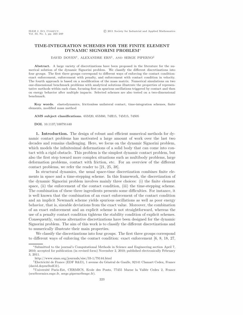
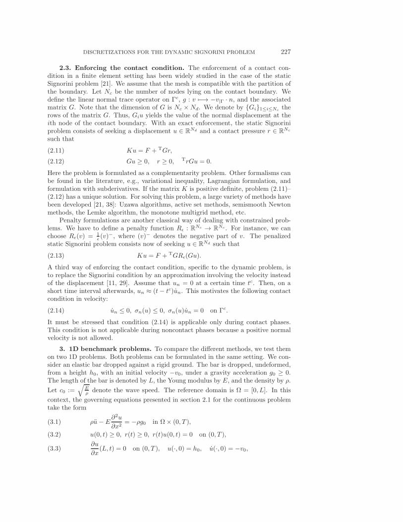
As illustrated in Figure 9, the large spurious oscillations have disappeared. How-ever, this stabilization takes effect only one step after the impact, which explainsthe peak in the contact pressure just after the impact. A possible remedy consistsof finding a time discretization where the contact force does not work or is at leastdissipative. For instance, the midpoint scheme with an enforcement of the contactcondition at time tn+1 (Discretization 4.4) achieves the following energy balance:

En+1 − En = Trn+1(Gun+1 −Gun) + TFn+ 12 (un+1 − un).

It is easy to check that the work of the contact force is always nonpositive. Asillustrated in Figure 10, the contact pressure still oscillates, but the stress is practicallyfree of oscillations. The oscillations of the stress after the bar has taken off are dueto vibrations. However, energy losses, even if they are not substantial, do have animpact on the solution (Figure 11). It can also be noticed that energy losses do notvanish as Δt approaches zero, but these losses decrease with the mesh size.

Discretization 4.4 (midpoint-implicit contact). Seek un+1, un+1 ∈ RNd , and

rn+1 ∈ RNc such that

Mun+ 12 +Kun+ 1

2 = Fn+ 12 + TGrn+1,(4.16)

Gun+1 ≥ 0, rn+1 ≥ 0, Trn+1Gun+1 = 0,(4.17)

un+1 = un +Δt un+ 12 ,(4.18)

un+1 = un +Δt un+ 12 .(4.19)


-2

-1

0

1

2

3

4

5

6

0 5 10 15 20

disp

lace

men

t

time


440

450

460

470

480

490

500

510

0 5 10 15 20

ener

gy

time



Discretization 4.4. Δx = 0.1, Δt = 0.005, νc = 1.5.

Another scheme with dissipative contact has been proposed in [18]. The Newmarkscheme with parameters β = 1/2 and γ = 1 and with an enforcement of the contactcondition at time tn+1 yields the following energy balance:

En+1−En = Trn+1(Gun+1−Gun)− 1

2T(un+1−un)K(un+1−un)+TFn+1(un+1−un).

The work of the contact force is always nonpositive, but there is a strong bulk dis-sipation. To remove this dissipation, one can, as proposed in [18], discretize theacceleration coming from the contact forces with the dissipative parameters (β = 1/2and γ = 1), and the acceleration coming from the elastic forces with a trapezoidal rule(β = 1/4 and γ = 1/2). This yields Discretization 4.5. With such a discretization,the energy balance is

En+1 − En = Trn+1(Gun+1 −Gun) + TFn+1(un+1 − un).

The numerical results are similar to those obtained with Discretization 4.4.Discretization 4.5 (Newmark with dissipative contact [18]). Seek un+1, un+1,

un+1int , un+1

con ∈ RNd , and rn+1 ∈ R

Nc such that

Mun+1 +Kun+1 = Fn+1 + TGrn+1,(4.20)

Gun+1 ≥ 0, rn+1 ≥ 0, Trn+1Gun+1 = 0,(4.21)


2un+2βint +

Δt2

2un+1con ,(4.22)

un+1 = un +Δtun+γint +Δtun+1

con ,(4.23)

where un+1 = un+1int + un+1

con and Mun+1con = TGrn+1.

To compensate for energy losses in schemes with dissipative contact, the so-calledvelocity-update method can be considered [27]. Applied to Discretization 4.4, thisprocedure does not significantly improve the solution on our second benchmark. In[8], the authors add to Discretization 4.5 a stabilization procedure (Discretization 4.6);for a consistency result under the assumption of viscoelastic material, see [22].

Discretization 4.6 (stabilized Newmark [8]).1. Seek un+1

pred ∈ RNd and λn+1 ∈ R

Nc such that

Mun+1pred = Mun +ΔtMun,(4.24)

Gun+1pred ≥ 0, λn+1 ≥ 0, Tλn+1Gun+1

pred = 0.(4.25)


2. Seek un+1, un+1, un+1int , un+1

con ∈ RNd , and rn+1 ∈ R

Nc satisfying (4.20), (4.21),and (4.23), while (4.22) is replaced by

un+1 = un+1pred +

Δt2

2un+2βint +

Δt2

2un+1con .(4.26)

The additional step required by Discretization 4.6 is not expensive compared withthe main step, especially if the mass matrix is lumped. With this scheme, the contactpressure is now almost free of oscillations (Figure 12). Although the impact law is not

fulfilled, Giun+2βint + Giu

n+1con = 0 holds true if Giu

n+1 = Giun+1pred = 0. Energy losses

still remain sizeable in the second benchmark (Figure 13).

-0.2

-0.1

0

0.1

0.2

0.3

0.4

0.4 0.5 0.6 0.7 0.8 0.9 1 1.1 1.2 1.3

disp

lace

men

t

time

ex./stabilized Newmarkexact solution

-100

0

100

200

300

400

500

0.4 0.5 0.6 0.7 0.8 0.9 1 1.1 1.2 1.3

cont

act p

ress

ure

time



Discretization 4.6 with β = 1/4 and γ = 1/2 (lumped mass matrix). Δx = 0.1, Δt = 0.005,νc = 1.5.

-2

-1

0

1

2

3

4

5

6

0 5 10 15 20

disp

lace

men

t

time


440

450

460

470

480

490

500

510

0 5 10 15 20

ener

gy

time



Discretization 4.6 with β = 1/4 and γ = 1/2 (lumped mass matrix). Δx = 0.1, Δt = 0.005,νc = 1.5.

4.2. Semiexplicit schemes. Now, we try to discretize the elastodynamics partof the problem with an explicit scheme, such as the central difference scheme. It isnot possible to enforce an explicit exact contact condition. Nevertheless, the contactcondition can be enforced implicitly as in [31, 32].

Discretization 4.7 (central differences-implicit contact [31, 32]). Seek un+1 ∈R

Nd and rn+1 ∈ RNc such that

M

(un+1 − 2un + un−1

Δt2

)+Kun = Fn + TGrn+1,(4.27)

Gun+1 ≥ 0, rn+1 ≥ 0, Trn+1Gun+1 = 0.(4.28)


With a lumped mass matrix, this scheme is equivalent to that proposed in [6]where the contact condition is enforced by a projection step in the following semiex-plicit way (observe that the first step is explicit):

1. Seek un+1 ∈ RNd such that

M

(un+1 − 2un + un−1

Δt2

)+Kun = Fn.(4.29)

2. If Giun+1 < 0, then un+1 is modified so that Giu

n+1 = 0.It is easy to check that, with Discretization 4.7, the acceleration at the contact bound-ary vanishes during a contact phase (after two steps). Indeed, if Giu

n+1 = Giun =

Giun−1 = 0, then Giu

n = Gi

(un+1−2un+un−1

Δt2

)= 0. Consequently, there are (almost)

no spurious oscillations (Figure 14). The shifted energy balance reads

En+10, 12

− En0, 12

= T

(rn+2 + rn+1

2

)(Gun+1 −Gun) + T

(Fn+1 + Fn

2

)(un+1 − un).

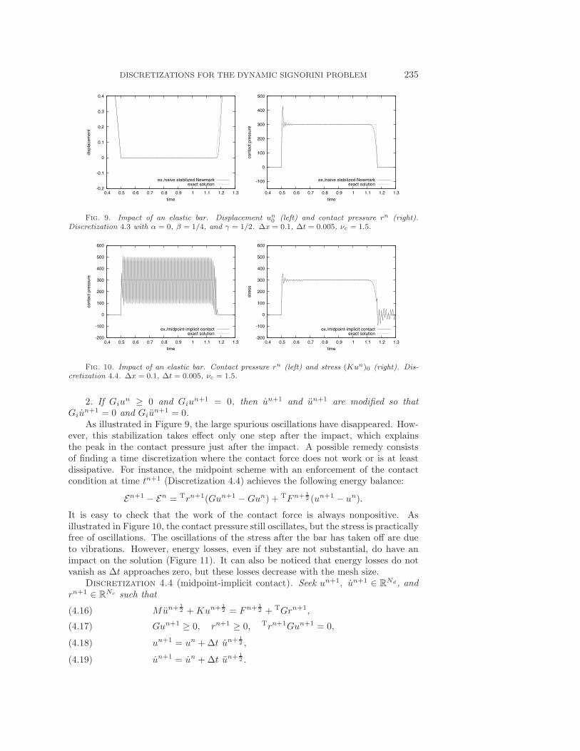
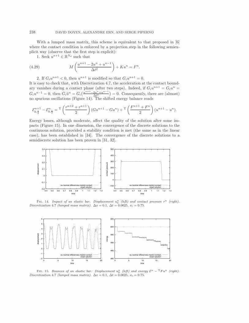
Energy losses, although moderate, affect the quality of the solution after some im-pacts (Figure 15). In one dimension, the convergence of the discrete solutions to thecontinuous solution, provided a stability condition is met (the same as in the linearcase), has been established in [34]. The convergence of the discrete solutions to asemidiscrete solution has been proven in [31, 32].

-0.2

-0.1

0

0.1

0.2

0.3

0.4

0.4 0.5 0.6 0.7 0.8 0.9 1 1.1 1.2 1.3

disp

lace

men

t

time

ex./central differences-implicit contactexact solution

-100

0

100

200

300

400

500

0.4 0.5 0.6 0.7 0.8 0.9 1 1.1 1.2 1.3

cont

act p

ress

ure

time



Discretization 4.7 (lumped mass matrix). Δx = 0.1, Δt = 0.0025, νc = 0.75.

-2

-1

0

1

2

3

4

5

6

0 5 10 15 20

disp

lace

men

t

time


480

485

490

495

500

505

0 5 10 15 20

ener

gy

time





-0.2

-0.1

0

0.1

0.2

0.3

0.4

0.4 0.5 0.6 0.7 0.8 0.9 1 1.1 1.2 1.3

disp

lace

men

t

time

pen./Newmarkexact solution

-100

0

100

200

300

400

500

0.4 0.5 0.6 0.7 0.8 0.9 1 1.1 1.2 1.3

cont

act p

ress

ure

time


Fig. 16. Impact of an elastic bar. Displacement un0 (left) and contact pressure TGRε(Gun)

(right). Discretization 5.1 with α = 0, β = 1/4, γ = 1/2, ε = 10−4. Δx = 0.1, Δt = 0.005, νc = 1.5.

-100

0

100

200

300

400

500

0.4 0.5 0.6 0.7 0.8 0.9 1 1.1 1.2 1.3

cont

act p

ress

ure

time


-500

0

500

1000

1500

2000

0.4 0.5 0.6 0.7 0.8 0.9 1 1.1 1.2 1.3

cont

act p

ress

ure

time


Fig. 17. Impact of an elastic bar. Contact pressure TGRε(Gun). Discretization 5.1 with α = 0,β = 1/4, and γ = 1/2. Δx = 0.1, Δt = 0.005, νc = 1.5. ε = 10−3 (left) and ε = 10−5 (right).

5. Discretizations with penalty contact condition. In this part we combinestandard finite elements in space and a penalty approximation of the contact condition(the penalty parameter is denoted by ε). Then, the semidiscrete problem is a meresystem of ODEs.

Problem 5.1. Seek a displacement u : [0, T ] → RNd such that, for all t ∈ [0, T ],

(5.1) Mu(t) +Ku(t) = f(t) + TGRε(Gu(t)),

with the initial conditions u(0) = u0 and u(0) = v0.Problem 5.1, being a system of ODEs with a Lipschitz continuous right-hand side,

has one and only one solution, which is furthermore twice differentiable in time.

5.1. Implicit schemes. To begin with, we discretize Problem 5.1 with an im-plicit Newmark scheme.

Discretization 5.1 (Newmark). Seek un+1, un+1, un+1 ∈ RNd , such that

Mun+1 +Kun+1 = Fn+1 + TGRε(Gun+1),(5.2)


2un+2β ,(5.3)

un+1 = un +Δtun+γ .(5.4)

We observe that the penalty formulation tends to reduce spurious oscillations(Figure 16). Nevertheless, the oscillations grow with 1/ε (Figure 17). This is not


-2

-1

0

1

2

3

4

5

6

0 5 10 15 20

disp

lace

men

t

time


460

470

480

490

500

510

0 5 10 15 20

ener

gy

time



Discretization 5.1 with α = 0, β = 1/4, γ = 1/2, and ε = 10−4. Δx = 0.1, Δt = 0.005, νc = 1.5.

surprising, since the penalty contact condition tends to the exact contact conditionwhen 1/ε tends to infinity. If the oscillations are too large, stabilization procedurescan be used (see, for instance, the procedure described in [1]). With the additionof a penalty term, the Newmark scheme (trapezoidal rule) no longer conserves theenergy. The energy losses are moderate but not so marginal (Figure 18); the energybehavior is poorer when 1/ε grows. In [1, 15], the authors proposed a discretizationof the penalty term which enables one to recover energy control by conserving anaugmented energy (Discretization 5.2). It is based on a midpoint scheme. On ourbenchmark problems, it does not yield significantly better results.

Discretization 5.2 (energy-controlling midpoint [1, 15]). Seek un+1, un+1 ∈R

Nd such that

Mun+ 12 +Kun+ 1

2 = Fn+ 12 + TGRε(Gun+1, Gun),(5.5)

un+1 = un +Δtun+ 12 ,(5.6)

un+1 = un +Δtun+ 12 ,(5.7)

where

(5.8) (Rε(Gun+1, Gun))i =

⎧⎪⎨⎪⎩

12ε

((Giun+1)−)2−((Giu

n)−)2

Giun+1−Giun if Giun �= Giu

n+1,

0 if Giun = Giu

n+1 ≥ 0,12ε (Gun+1 +Gun) if Giu

n = Giun+1 < 0.

Defining the augmented energy Enpen := En + 1

2ε((Gun)−)2, there holds

En+1pen − En

pen = TFn+ 12 (un+1 − un).

Since Enpen is an upper bound of En, controlling En

pen allows one to control En.

5.2. Explicit schemes. We can also use an explicit scheme for Problem 5.1.Discretization 5.3 (central differences). Seek un+1 ∈ R

Nd such that

M

(un+1 − 2un + un−1

Δt2

)+Kun = Fn + TGRε(Gun).(5.9)

The results are similar to those obtained with the implicit approach. Unfortu-nately, the penalty term stiffens the system of ODEs, which limits the stability domainof the schemes. More precisely, it introduces a constraint on the time step of the formΔt ≤ O(

√ρεΔxc), where Δxc is the mesh size near the contact boundary [3].


6. Discretizations with contact condition in velocity. In this section, stan-dard finite elements in space are combined with an approximation of the contactcondition involving the velocity.

Problem 6.1. Seek a displacement u : [0, T ] → RNd and a contact pressure

r : [0, T ] → RNc such that, for almost every t ∈ [0, T ],

Mu(t) +Ku(t) = f(t) + TGr(t),(6.1)

Gu(t) ≥ 0, r(t) ≥ 0, Tr(t)Gu(t) = 0,(6.2)

with the initial conditions u(0) = u0 and u(0) = v0.With this contact condition in velocity, the semidiscrete problem is much simpler

than (4.1)–(4.2). Problem 6.1 is still a system of ODEs under unilateral constraints,but the constraint now involves the velocity instead of the displacement. The generaltheory developed in [4, 12] applies to Problem 6.1. The solution u is unique [4].Furthermore, u is continuous and u is differentiable in time almost everywhere, sothat the equations have a sense at almost every time. The time discretization hasbeen extensively studied in [12].

Unfortunately, the contact condition in velocity is not equivalent to the Signorinicondition as discussed in section 2.3. The strategy adopted is the following: if a nodesatisfies the noninterpenetration condition, then at the next iteration no constraintis enforced on this node; if a node breaks the noninterpenetration condition, then atthe next iteration the contact condition in velocity will be applied to this node. Thisapproach allows for slight interpenetration. At each time step, we define the matrixGn whose rows Gn

i are

(6.3) Gni =

{(0 . . . 0) if Giu

n ≥ 0,

Gi if Giun < 0.

This approach based on a contact condition in velocity has also been widely used inrigid-body dynamics with impacts (see, e.g., [35]).

6.1. Implicit schemes. A midpoint scheme with contact condition in velocityhas been proposed in [26]; see also [19] for the contact condition.

Discretization 6.1 (midpoint [26]). Seek un+1, un+1 ∈ RNd , and rn+1 ∈ R

Nc

such that

Mun+ 12 +Kun+ 1

2 = Fn+ 12 + TGnrn+

12 ,(6.4)

Gnun+ 12 ≥ 0, rn+

12 ≥ 0, Trn+

12Gnun+ 1

2 = 0,(6.5)

un+1 = un +Δt un+ 12 ,(6.6)

un+1 = un +Δt un+ 12 .(6.7)

An interesting feature of this scheme is to be energy-conserving,

En+1 − En = TFn+ 12 (un+1 − un).

The contact pressure does not perturb the structure despite its oscillations (Figure 19).Energy is preserved, and the solution for the second benchmark is quite satisfactory,although not as accurate as with Discretization 5.1 after several impacts (Figure 20).


-0.2

-0.1

0

0.1

0.2

0.3

0.4

0.4 0.5 0.6 0.7 0.8 0.9 1 1.1 1.2 1.3

disp

lace

men

t

time

vel./midpointexact solution

-100

0

100

200

300

400

500

0.4 0.5 0.6 0.7 0.8 0.9 1 1.1 1.2 1.3

cont

act p

ress

ure

time


Fig. 19. Impact of an elastic bar. Displacement un0 (left) and stress (right). Discretization 6.1

with α = 0, β = 1/4, and γ = 1/2. Δx = 0.1, Δt = 0.005, νc = 1.5.

-2

-1

0

1

2

3

4

5

6

0 5 10 15 20

disp

lace

men

t

time


498

498.5

499

499.5

500

500.5

501

0 5 10 15 20

ener

gy

time




6.2. Semiexplicit schemes. A semiexplicit scheme with contact condition invelocity has been proposed in [3].

Discretization 6.2 (central differences [3]). Seek un+1 ∈ RNd and rn+1 ∈ R

Nc

such that

M

(un+1 − 2un + un−1

Δt2

)+Kun = Fn + TGnrn+1,(6.8)

Gn(un+1 − un) ≥ 0, rn+1 ≥ 0, Trn+1Gn(un+1 − un) = 0.(6.9)

Numerical simulations suggest that the stability condition of the central differencescheme is not tightened by the contact condition. The results are similar to thoseobtained with Discretization 4.7 (Figures 21 and 22).

7. Discretizations with modified mass. In the previous three sections, wehave considered various ways of enforcing the contact condition. Here we describemethods based on a modification of the mass matrix. Such methods are thus compat-ible with any enforcement of the contact condition. For brevity, we restrict ourselvesto an exact enforcement of the contact condition. In the modified mass matrix, theentries associated with the normal displacements at the contact boundary are set tozero. The motivation for this modification is very simple: if the mass is removed,the inertial forces and the oscillations are eliminated. This approach was introducedin [20].

Set N∗d := Nd − Nc. For the sake of simplicity, suppose that the degrees of

freedom associated with normal displacements at the contact boundary are numbered


-0.2

-0.1

0

0.1

0.2

0.3

0.4

0.4 0.5 0.6 0.7 0.8 0.9 1 1.1 1.2 1.3

disp

lace

men

t

time

vel./central differencesexact solution

-100

0

100

200

300

400

500

0.4 0.5 0.6 0.7 0.8 0.9 1 1.1 1.2 1.3

cont

act p

ress

ure

time




-2

-1

0

1

2

3

4

5

6

0 5 10 15 20

disp

lace

men

t

time


480

485

490

495

500

505

0 5 10 15 20

ener

gy

time




from N∗d + 1 to Nd. The modified mass matrix is defined as

M∗ =

(M∗∗ 00 0

).

Many choices are possible in building the block M∗∗. In [14, 20], the authors devisevarious methods for preserving some features of the standard mass matrix (the totalmass, the center of gravity, and the moments of inertia); see also [33] for further results.We can also simply keep the corresponding block in the standard mass matrix (andthis is what we will do in our numerical simulations below). The modified problemreads

M∗u(t) +Ku(t) = F (t) + TGr(t),(7.1)

Gu(t) ≥ 0, r(t) ≥ 0, Tr(t)Gu(t) = 0.(7.2)

If we set u(t) =(u∗(t)uc(t)

), K =

(K∗∗Kc∗

K∗cKcc

), F (t) =

(F∗(t)Fc(t)

), and G = (0 Gc), then (7.1)

and (7.2) can be recast as

M∗∗u∗(t) +K∗∗u∗(t) +K∗cuc(t) = F∗(t),(7.3)

Kc∗u∗(t) +Kccuc(t) = Fc(t) +TGcr(t),(7.4)

Gcuc(t) ≥ 0, r(t) ≥ 0, Tr(t)Gcuc(t) = 0.(7.5)


For given t and u∗(t), there exists one and only one uc(t) satisfying (7.4) and (7.5).Denote by Q : [0, T ]× R

N∗d → R

Nc the nonlinear map such that uc(t) = Q(t, u∗(t)).Problem 7.1. Seek a displacement u : [0, T ] → R

Nd such that, for all t ∈ [0, T ],

M∗∗u∗(t) +K∗∗u∗(t) +K∗cQ(t, u∗(t)) = F∗(t),(7.6)

uc(t) = Q(t, u∗(t)),(7.7)

with the initial conditions u(0) = u0 and u(0) = v0.The operator Q(t, ·) is Lipschitz continuous at each time t, so that (7.6) is a

Lipschitz system of ODEs. Therefore, it has a unique solution u∗, twice differentiablein time. Owing to (7.7), uc is differentiable in time almost everywhere. The detailedmathematical analysis of the space semidiscrete modified mass formulation can befound in [20, 9]. A result of convergence of the space semidiscrete solutions to acontinuous solution is proven for viscoelastic materials in [9].

Remark 7.1. In contrast to the semidiscrete problem with standard mass matrix,the semidiscrete problem with modified mass matrix does not require an impact lawand conserves a modified energy where the mass modification is accounted for in thekinetic energy [20].

7.1. Implicit schemes. An HHT-Newmark scheme can be used for Problem 7.1.Discretization 7.1 (HHT-Newmark [20]). Seek un+1 ∈ R

Nd, un+1∗ ∈ R

Nd, andun+1∗ ∈ R

Nd such that

M∗∗un+1∗ +K∗∗un+1+α

∗ +K∗cQ(tn+1+α, un+1+α∗ ) = Fn+1+α

∗ ,(7.8)

un+1+αc = Q(tn+1+α, un+1+α

∗ ),(7.9)

un+1∗ = un

∗ +Δtun∗ +

Δt2

2un+2β∗ ,(7.10)

un+1∗ = un

∗ +Δtun+γ∗ .(7.11)

The equations can be recast as a linear complementarity problem,

M∗un+1 +Kun+1+α = Fn+1+α + TGrn+1,(7.12)

Gun+1 ≥ 0, rn+1 ≥ 0, Trn+1Gun+1 = 0,(7.13)


2un+2β ,(7.14)

un+1 = un +Δtun+γ .(7.15)

In spite of the modification of the mass matrix, the problem is well-posed. In practice,we use this set of equations to compute the solution. As expected, the large oscillationshave disappeared during the contact phase (Figure 23). The energy behavior is alsovery satisfactory (Figure 24), since

En+1∗ − En

∗ = T

(rn+1 + rn

2

)(Gun+1 −Gun) + T

(Fn+1 + Fn

2

)(un+1 − un),

where the modified energy En∗ has the same expression as En, except thatM is replacedby M∗. The displacement after several impacts is quite satisfactory, although not asaccurate as with Discretization 5.1 (Figure 24).


-0.2

-0.1

0

0.1

0.2

0.3

0.4

0.4 0.5 0.6 0.7 0.8 0.9 1 1.1 1.2 1.3

disp

lace

men

t

time

mass/Newmarkexact solution

-100

0

100

200

300

400

500

0.4 0.5 0.6 0.7 0.8 0.9 1 1.1 1.2 1.3

cont

act p

ress

ure

time


Fig. 23. Impact of an elastic bar. Displacement un0 and contact pressure rn. Discretization 7.1

with α = 0, β = 1/4, and γ = 1/2. Δx = 0.1, Δt = 0.005, νc = 1.5.

-2

-1

0

1

2

3

4

5

6

0 5 10 15 20

disp

lace

men

t

time


494

495

496

497

498

499

500

501

502

0 5 10 15 20

ener

gy

time


Fig. 24. Bounces of an elastic bar. Displacement un0 (left) and modified energy En∗ − TFun

(right). Discretization 7.1 with α = 0, β = 1/4, and γ = 1/2. Δx = 0.1, Δt = 0.005, νc = 1.5.

7.2. Semiexplicit schemes. We can discretize Problem 7.1 with an explicitscheme, such as the central difference scheme. This yields a semiexplicit scheme.

Discretization 7.2 (central differences [10]). Seek un+1 ∈ RNd such that

M∗∗

(un+1∗ − 2un∗ + un−1∗

Δt2

)+K∗∗un

∗ +K∗cQ(tn, un∗ ) = Fn

∗ ,(7.16)

un+1c = Q(tn+1, un+1

∗ ).(7.17)

In practice, the equations are solved as follows: 1. Seek un+1∗ ∈ RNd such that

(7.18) M∗∗

(un+1∗ − 2un

∗ + un−1∗

Δt2

)+K∗∗un

∗ +K∗cunc = Fn

∗ .

2. Seek un+1c ∈ R

N∗d and rn+1 ∈ R

Nc such that

Kc∗un+1∗ +Kccu

n+1c = Fn+1

c + TGcrn+1,(7.19)

Gcun+1c ≥ 0, rn+1 ≥ 0, TrGcu

n+1c = 0.(7.20)

The first step is explicit, and the mass matrix M∗∗ can be lumped. The second stepis a constrained problem on the variable un+1

c only. Discretization 7.2 amounts to

M∗(un+1 − 2un + un−1

Δt2

)+Kun = Fn + TGrn,

Gun ≥ 0, rn ≥ 0, TrnGun = 0,


-2

-1

0

1

2

3

4

5

6

0 5 10 15 20

disp

lace

men

t

time

mass/central differencesexact solution

498

498.5

499

499.5

500

500.5

501

0 5 10 15 20

ener

gy

time

mass/central differencesexact solution

Fig. 25. Bounces of an elastic bar. Displacement un0 (left) and modified energy En∗ − TFun

(right). Discretization 7.2 (lumped mass matrix). Δx = 0.1, Δt = 0.0025, νc = 0.75.

��

O

R g0

ΩΓc

Fig. 26. Bounces of an elastic disk. Reference configuration (left), mesh (middle), and de-formed configuration after the first impact (right).

and yields the modified shifted energy balance

En+10, 12∗

− En0, 12 ∗ = T

(rn+1 + rn

2

)(Gun+1 −Gun) + T

(Fn+1 + Fn

2

)(un+1 − un),

where En0, 12∗

has the same expression than En0, 12

, except that M is replaced by M∗. We

observe numerically that the stability condition on the time step is the same as in thelinear case. Compared with Discretizations 4.7 and 6.2, the semiexplicit modified massmethod shows a better energy behavior and a better solution (Figure 25). Additionaltests show that the amplitude of energy oscillations decreases at least linearly withΔt at fixed Courant number. Results on the first benchmark are similar to those withthe implicit scheme.

8. A 2D benchmark. We consider the bounces of an elastic disk against a rigidground (Figure 26). The reference configuration is the undeformed disk touching theground. The disk is dropped, undeformed, with a zero initial velocity, under a gravityacceleration g0, the displacement of its center being initially h0. The disk has radiusR.The material is supposed to be linear elastic (plane strain) with a Young modulus E,a Poisson ratio ν, and a mass density ρ. The contact boundary Γc is the lower halfof the disk boundary. We define the contact condition using the normal vector to theground. The parameters are E = 4000, ν = 0.2, ρ = 100, g0 = 5, R = 1, h0 = 0.1.The disk is meshed with triangles (100 edges on the boundary, 1804 triangles, 953vertices; see Figure 26) and we use linear finite elements. The number of nodeslying on the contact boundary is 51. Simulations are performed using FreeFem++

[16]. The Courant number is defined as νc := cdΔxΔt , where cd = 20

3 is the speed ofdilatational waves and Δx = 0.0628 the length of boundary edges.


-0.8

-0.6

-0.4

-0.2

0

0.2

0 2 4 6 8 10

disp

lace

men

t

time

mass/Newmarkex./stabilized Newmark

vel./midpoint 80

90

100

110

120

130

140

150

160

170

0 2 4 6 8 10

ener

gy

time

mass/Newmarkex./stabilized Newmark

vel./midpoint

Fig. 27. Bounces of an elastic disk. Displacement of its center (left) and energy or modifiedenergy (right). Discretizations 4.6, 6.1, and 7.1. Δt = 0.01, νc = 1.06.

-0.8

-0.6

-0.4

-0.2

0

0.2

0 2 4 6 8 10

disp

lace

men

t

time

mass/central differencesex./central differences-implicit contact

120

125

130

135

140

145

150

155

160

0 2 4 6 8 10

ener

gy

time

mass/central differencesex./central differences-implicit contact

Fig. 28. Bounces of an elastic disk. Displacement of its center (left) and energy or modifiedenergy (right). Discretizations 4.7 and 7.2. Δt = 0.005, νc = 0.53.

Results are presented for the implicit Discretizations 4.6, 6.1, and 7.1 (Figure 27)and for the semiexplicit Discretizations 4.7 and 7.2 (Figure 28). For the semiexplicitschemes, the observed stability condition is νc ≤ 0.65. In all cases, the trajectoryof the disk center is rather well captured, with some discrepancies appearing afterfive bounces. The energy behaviors remain consistent with those observed in onedimension. Note that the present choice of parameters is somewhat severe for energybehavior because of the relatively high impact velocity and low Young modulus.

9. Conclusions. In this work, we have reviewed various time-integration schemesfor the finite element dynamic Signorini problem. We have classified the schemes intofour groups, the first three depending on the way the contact condition is enforcedwhile the fourth group corresponds to modifying the mass matrix at the contactboundary. We have tested in detail the various schemes on two 1D benchmarks, bothwith analytical solution. The second benchmark is new and allows one to study theenergy behavior within multiple impacts. Some selected schemes with favorable prop-erties have been further compared on a 2D benchmark. All in all, we believe that theschemes with modified mass matrix, either implicit or semiexplicit, offer attractiveproperties, including ease of implementation, robustness, and relatively firm mathe-matical ground. The semiexplicit scheme with modified mass is new and stems fromthe combination of two existing ideas. We hope that the present results will stimulatefurther interest in the analysis and testing of these schemes.


REFERENCES

[1] F. Armero and E. Petocz, Formulation and analysis of conserving algorithms for frictionlessdynamic contact/impact problems, Comput. Methods Appl. Mech. Engrg., 158 (1998),pp. 269–300.

[2] Y. Ayyad, M. Barboteu, and J. Fernandez, A frictionless viscoelastodynamic contact prob-lem with energy consistent properties: Numerical analysis and computational aspects,Comput. Methods Appl. Mech. Engrg., 198 (2009), pp. 669–679.

[3] T. Belytschko and M. Neal, Contact-impact by the pinball algorithm with penalty and La-grangian methods, Internat. J. Numer. Methods Engrg., 31 (1991), pp. 547–572.

[4] H. Brezis and J.-L. Lions, Sur certains problemes unilateraux hyperboliques, C. R. Acad. Sci.Paris Ser. A, 264 (1967), pp. A928–A931.

[5] B. Brogliato, Nonsmooth Impact Mechanics, Springer-Verlag, London, 1996.[6] N. Carpenter, R. Taylor, and M. Katona, Lagrange constraints for transient finite element

surface contact, Internat. J. Numer. Methods Engrg., 32 (1991), pp. 103–128.[7] R. Courant and D. Hilbert, Methods of Mathematical Physics. Vol. I, Interscience, New

York, 1953.[8] P. Deuflhard, R. Krause, and S. Ertel, A contact-stabilized Newmark method for dynamical

contact problems, Internat. J. Numer. Methods Engrg., 73 (2008), pp. 1274–1290.[9] D. Doyen and A. Ern, Convergence of a space semi-discrete modified mass method for the

dynamic Signorini problem, Commun. Math. Sci., 7 (2009), pp. 1063–1072.[10] D. Doyen, A. Ern, and S. Piperno, A Semi-explicit Modified Mass Method for Dynamic

Contact Problems, Lectures Notes in Appl. Comput. Mech., Springer, New York, 2010.[11] C. Eck, J. Jarusek, and M. Krbec, Unilateral Contact Problems. Variational Methods and

Existence Theorems, Chapman & Hall/CRC, Boca Raton, FL, 2005.[12] R. Glowinski, J.-L. Lions, and R. Tremolieres, Numerical Analysis of Variational Inequal-

ities, North–Holland, Amsterdam, 1981.[13] E. Grosu and I. Harari, Stability of semidiscrete formulations for elastodynamics at small

time steps, Finite Elem. Anal. Des., 43 (2007), pp. 533–542.[14] C. Hager, S. Hueber, and B. I. Wohlmuth, A stable energy-conserving approach for fric-

tional contact problems based on quadrature formulas, Internat. J. Numer. Methods Engrg.,73 (2008), pp. 205–225.

[15] P. Hauret and P. Le Tallec, Energy-controlling time integration methods for nonlinearelastodynamics and low-velocity impact, Comput. Methods Appl. Mech. Engrg., 195 (2006),pp. 4890–4916.

[16] F. Hecht and O. Pironneau, FreeFEM++, software, available online from www.freefem.org.[17] T. J. R. Hughes, The Finite Element Method, Prentice–Hall, Englewood Cliffs, NJ, 1987.[18] C. Kane, E. A. Repetto, M. Ortiz, and J. E. Marsden, Finite element analysis of non-

smooth contact, Comput. Methods Appl. Mech. Engrg., 180 (1999), pp. 1–26.[19] H. B. Khenous, P. Laborde, and Y. Renard, Comparison of two approaches for the dis-

cretization of elastodynamic contact problems, C. R. Math. Acad. Sci. Paris, 342 (2006),pp. 791–796.

[20] H. B. Khenous, P. Laborde, and Y. Renard, Mass redistribution method for finite elementcontact problems in elastodynamics, Eur. J. Mech. A Solids, 27 (2008), pp. 918–932.

[21] N. Kikuchi and J. T. Oden, Contact Problems in Elasticity: A Study of Variational Inequal-ities and Finite Element Methods, SIAM Stud. Appl. Math. 8, SIAM, Philadelphia, PA,1988.

[22] C. Klapproth, A. Schiela, and P. Deuflhard, Consistency results for the contact-stabilizedNewmark method, Numer. Math., 116 (2010), pp. 65–94.

[23] R. Krause and M. Walloth, Presentation and Comparison of Selected Algorithms for Dy-namic Contact Based on the Newmark Scheme, technical report, Institute of Computa-tional Science, Universita della Svizzera italiana, 2009.

[24] S. Krenk, Energy conservation in Newmark based time integration algorithms, Comput. Meth-ods Appl. Mech. Engrg., 195 (2006), pp. 6110–6124.

[25] T. A. Laursen, Computational Contact and Impact Mechanics, Springer-Verlag, Berlin, 2002.[26] T. A. Laursen and V. Chawla, Design of energy conserving algorithms for frictionless dy-

namic contact problems, Internat. J. Numer. Methods Engrg., 40 (1997), pp. 863–886.[27] T. A. Laursen and G. R. Love, Improved implicit integrators for transient impact problems—

Geometric admissibility within the conserving framework, Internat. J. Numer. MethodsEngrg., 53 (2002), pp. 245–274.

[28] G. Lebeau and M. Schatzman, A wave problem in a half-space with a unilateral constraintat the boundary, J. Differential Equations, 53 (1984), pp. 309–361.


[29] J. J. Moreau, Numerical aspects of the sweeping process. Computational modeling of contactand friction, Comput. Methods Appl. Mech. Engrg., 177 (1999), pp. 329–349.

[30] N. Nsiampa, J.-P. Ponthot, and L. Noels, Comparative study of numerical explicit schemesfor impact problems, Internat. J. Impact Engrg., 35 (2008), pp. 1688–1694.

[31] L. Paoli and M. Schatzman, A numerical scheme for impact problems. I: The one-dimensionalcase, SIAM J. Numer. Anal., 40 (2002), pp. 702–733.

[32] L. Paoli and M. Schatzman, A numerical scheme for impact problems. II: The multidimen-sional case, SIAM J. Numer. Anal., 40 (2002), pp. 734–768.

[33] Y. Renard, The singular dynamic method for constrained second order hyperbolic equations:Application to dynamic contact problems, J. Comput. Appl. Math., 234 (2010), pp. 906–923.

[34] M. Schatzman and M. Bercovier, Numerical approximation of a wave equation with unilat-eral constraints, Math. Comp., 53 (1989), pp. 55–79.

[35] D. E. Stewart, Rigid-body dynamics with friction and impact, SIAM Rev., 42 (2000), pp. 3–39.[36] R. Taylor and P. Papadopoulos, On a finite element method for dynamic contact/impact

problems, Internat. J. Numer. Methods Engrg., 36 (1993), pp. 2123–2140.[37] D. Vola, E. Pratt, M. Jean, and M. Raous, Consistent time discretization for dynami-

cal contact problems and complementarity techniques, Rev. Europ. Elem. Finis, 7 (1998),pp. 149–162.

[38] P. Wriggers, Computational Contact Mechanics, John Wiley & Sons, New York, 2002.

time-integration schemes for the finite …cermics.enpc.fr/~ern/pdfs/11_dep_sisc.pdf ·...

Documents