time explicit schemes and spatial finite differences ...bcosta/papers/fulltext.pdftime explicit...

159

0885-7474/04/0400-0159/0 © 2004 Plenum Publishing Corporation

Journal of Scientific Computing, Vol. 20, No. 2, April 2004 (© 2004)

Time Explicit Schemes and Spatial Finite DifferencesSplittings

Jean-Paul Chehab1 and Bruno Costa2

1 Laboratoire de Mathématiques Appliqués, (CNRS) FRE 2222, équipe ANO, Université deLille, France. E-mail: [email protected] and Laboratoire de Mathématiques,CNRS, UMR 8628, Equipe ANEDP, Université Paris Sud, Orsay, France.

2 Departamento de Matematica Aplicada, IM-UFRJ, Brazil. E-mail: [email protected]

Received April 11, 2002; accepted (in revised form) October 25, 2002

In this article, we conjugate time marching schemes with Finite Differencessplittings into low and high modes in order to build fully explicit methods withenhanced temporal stability for the numerical solutions of PDEs. The main ideais to apply explicit schemes with less restrictive stability conditions to the linearterm of the high modes equation, in order that the allowed time step for thetemporal integration is only determined by the low modes. These conjugatedschemes were developed in [10] for the spectral case and here we adapt them tothe Finite Differences splittings provided by Incremental Unknowns, whichsteems from the Inertial Manifolds theory. We illustrate their improved capa-bilities with numerical solutions of Burgers equations, with uniform and non-uniform meshes, in dimensions one and two, when using modified Forward–Euler and Adams–Bashforth schemes. The resulting schemes use time steps ofthe same order of those used by semi-implicit schemes with comparableaccuracy and reduced computational costs.

KEY WORDS: Finite differences; stability; incremental unknowns; multilevelschemes; Burgers equation.

1. INTRODUCTION

The modelization of the long time behavior of dissipative dynamicalsystems has gained new strength with the appearance of the concept ofinertial manifolds (see [24] and the references therein). The numericalmethods that emerged since then, namely, the Nonlinear Galerkin methods(NLG) [19], have intensively used the revealed interaction between the

large and small structures of a flow to achieve reduction of computationalcosts by proposing splittings of the solution into blocks (or levels) ofunknowns and treating them differently in the numerical process. Thesesplittings are naturally obtained in the spectral case or can be built by theuse of a suitable change of variables, as in the finite elements or finite dif-ferences cases [20, 25]. In these different situations, subsequent gain ofstability and accuracy have been reported: in [11] for the spectral methodssimulation of homogeneous turbulence; in [2] for Finite Elements appliedto Burgers and Navier–Stokes Equations (NSE) and in [23] and [21] forthe Finite Differences case. In this work we do not make use of theApproximate Inertial Manifold concept [19] in order to enslave the highfrequencies to the small ones. We only keep the essential idea of treatingdifferently the low and high modes through the NLG spatial splittings,aiming at a fully explicit method able to decrease the great computationalcosts of dissipative problems, which are due to the presence of a wide rangeof time scales.

Multiple time scales arise in many physical systems such as the onesinvolving controllers, chemical reactions or geophysical processes. Forinstance, Rossby waves in the Shalow–Water system move in a muchslower space than the faster gravity waves. Although the first ones carrymost of the physical energy, the latest are the ones to determine the tem-poral stability of an approximating numerical scheme. Analogously, thereare many other physical systems where perturbations of solutions evolve ina much faster time scale than the solution itself. The main consequence ofthis fact for the process of obtaining a computational solution translatesinto what numerical analists call stiffness. When using explicit schemes forsuch problems, either none or too many digits of accuracy are obtained,since the size of the time step is constrained not only by accuracy require-ments, but must also obey absolute stability restrictions (see [1]). In thisarticle we present a simple framework for fully explicit time schemes to beapplied on linear and nonlinear problems where we propose to substitutethe common use of implicit discretizations of the linear term by lessrestrictive (consequently, less precise) explicit schemes which allow the useof larger time steps. The separation of scales play an important role for weonly use such schemes on the low energy high frequencies. This approachhas been originally proposed in [10] where a spectral discretization wasconsidered. Here we concentrate on finite differences splittings for theanalysis of the schemes and the numerical experiments, however, ourapproach allows to consider other splittings, such as Hierachical basis infinite elements.

Time step restrictions originate from two main sources (disregardingboundary conditions): the discretized differential operator of the linear

160 Chehab and Costa

term might have large eigenvalues implying on rapidly decaying frequen-cies, or strong advection from the nonlinear terms (the CFL condition). Inthis article we restrict our attention to increase the time step bounds arisingfrom the dissipative linear term. We perform the numerical analysis of theproposed schemes applied in the linear case. Analytical results with numer-ical solutions of linear and nonlinear equations, where the nonlinear termsare also treated explicitly are also presented. Although, for general non-linear problems, we will also have a dependence of the time step on thenonlinear terms, the numerical results show computational advantages evenin the case of a weak dissipation.

This article is organized as follows: In Sec. 2 we derive the modifiedtime integration schemes starting in spectral space and extending to ageneral spatial hierarchization of scales. Section 3 presents the decomposi-tion of scales in finite differences by reviewing the construction of secondand fourth order Incremental Unknowns. In Sec. 4 we perform the stabilityanalysis of the modified schemes and discuss the choice of the associatedparameters. Finally, in Sec. 5, we present numerical results on the applica-tion of the modified Forward–Euler and Adams–Bashforth schemes to theBurgers equation in space dimensions one and two when using uniformand nonuniform grids with second and fourth order IUs.

2. TIME INTEGRATION SCHEMES

An elegant way of getting rid of the stifness of the linear term is theuse of exact integrating factors. For instance, consider the viscous Burgersequation

ut − uxx − 12 (u2)x=0 (1)

and its representation in the Fourier space

ddt

uk+k2uk+ik2

(u2)k=0. (2)

Making use of the integrating factor ek2t, we get

ddt

(ek2tuk)+ik2

(u2)k ek2t=0, (3)

yielding the following discrete equation (after a Forward–Euler discretization)

un+1k =e−k2

Dtunk −

ik Dt2

(u2)nk e−k2

Dt, (4)

Time Explicit Schemes and Spatial Finite Differences Splittings 161

with no time step restriction coming from the linear term, however suffer-ing from a fast decreasing coefficient in the nonlinear term, resulting on amilder, but still strong limitation on Dt (see also [15]).

In [10], it was proposed to consider instead the change of variable

w=ebtu, b > 0, (5)

for decreasing the size of the eigenvalues of the second derivative operator.For the sake of simplicity, let us apply the above transformation only tothe linear part of (1) ut − uxx=0, obtaining

wt=wxx+bw. (6)

This means that in frequency space

ddt

wk=−(k2 − b) wk,

and we can easily see that b > 0 decreases the size of the second derivativeeigenvalues, allowing faster temporal integration in the variable w. How-ever, to avoid the exponential growing of transformation (5), Eq. (6) isintegrated only one step in time and the original variable u is recovered atthe end of the iteration as the following algorithm shows:

• Step 1: Let w0=u0;

• Step 2: Apply the Forward–Euler discretization in Eq. (6):

w1=(1+b Dt) w0+Dt Dxxw1; (7)

• Step 3: Recover u1 by:

u1=w1 − b Dt u1. (8)

In [10], the scheme above was denominated the implicit correction,due to step 3, and it can be expressed as the single equation:

un+1=1+b Dt+Dt Dxx

1+b Dtun. (9)

The above scheme is explicit and is equivalent to the application of theForward–Euler scheme to the modified equation

(1+b Dt) ut=uxx. (10)


It is easy to see that if the N first modes are considered, then for b \ N2

2 ,this last scheme is unconditionnaly stable while keeping the same steady-states as the original equation.

In [10] the time marching scheme (9) was used in conjunction with ascales splitting in spectral methods and applied to the high frequenciesequation to generate an explicit scheme with stability restriction determinedby the low frequencies only. A thourough error analysis was undertakenshowing that for the maximum time step allowed by the low modes, scheme(9) is first order in time. The numerical experiments showed a successfullreduction in CPU time costs for linear and nonlinear problems where thelinear restriction on the time step is stronger than the CFL conditionarising from the nonlinear terms. All terms were treated explicitly.

Here, we adapt these ideas to the case of a separation of scales in finitedifferences provided by the Incremental Unknowns method, where greaterimprovement in the efficiency of the scheme is expected, since, distinctlyfrom the spectral case, the spatial errors are relevant. Below, in order topresent the overall framework to the reader, we show how the schemeworks in the case of a general change of variables (Hierarchical bases in theFinite Elements case are also included), leaving the more specific aspects ofthe IU discretization to Sec. 4, where we perform a detailed stability anal-ysis, in the linear case.

We hence consider the decomposition of the solution into d+1 arrays(or block of components) and denote by S the transfer matrix; when S is aFFT operator, the spectral framework is recovered, but other discretiza-tions can be considered. We start by writing the equation on the new basis

Xt+AX=F,

where A is the discretization matrix of − D, F the source term and

X=S Ryn+1

zn+11

·zn+1

d

S .

From the previous discussion, we want to apply scheme (9) only on theequations corresponding to the small structures, as below:

Ryn+1

zn+11

·zn+1

d

S=Ryn

zn1

·zn

d

S− Dt G RS−1AS Ryn

zn1

·zn

d

S− S−1FS , (11)


with

G=RId 0 · 0

01

1+Dt b1Id · 0

· · · ·

0 0 ·1

1+Dt bdId

S .

We define (11) as the Modified Forward Euler (MFE) scheme. Note thatdifferent values of b can be used for each level of the small scales.

Remark 2.1. The implicit correction of Step 3 can be improved inorder to generate a scheme with temporal consistency. For instance,substitution of Step 3 by

• Step 3 −: Recover u1 by:

u1=w1 − b Dt(u1+u−1)

2; (12)

yields the scheme

un+1 − un

Dt+b(un+1 − un)=un

xx+b(un − un − 1),

which approximates the equation ut+b Dt utt=uxx. In general, assumingthat the solution is smooth enough in time, we can consider the timeconsistent modified equation:

“u“t

+b(Dt)q “qu

“tq=uxx

and obtain schemes with enhanced stability and same steady states as theoriginal equation. However, more points in time have to be considered as qincreases.

2.1. Extension to Linear multistep methods

Consider the family of Adams–Bashforth schemes:

un+1 − un

Dt= C

p

j=0ajN

jFn


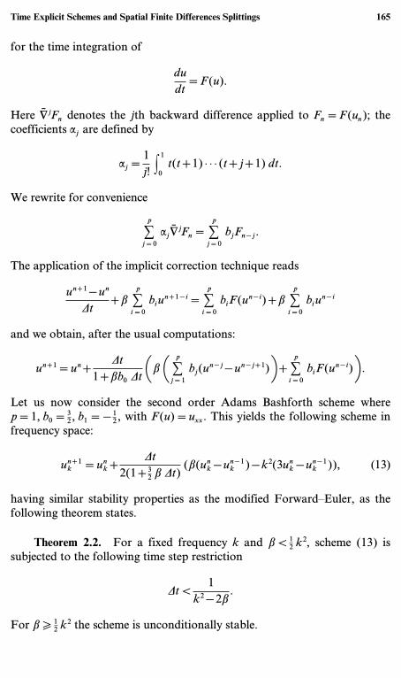
for the time integration of

dudt

=F(u).

Here N jFn denotes the jth backward difference applied to Fn=F(un); thecoefficients aj are defined by

aj=1j!

F1

0t(t+1) · · · (t+j+1) dt.

We rewrite for convenience

Cp

j=0ajN

jFn= Cp

j=0bjFn − j.

The application of the implicit correction technique reads

un+1 − un

Dt+b C

p

i=0biun+1 − i= C

p

i=0biF(un − i)+b C

p

i=0biun − i

and we obtain, after the usual computations:

un+1=un+Dt

1+bb0 Dt1b 1 C

p

j=1bj(un − j − un − j+1)2+ C

p

i=0biF(un − i)2 .

Let us now consider the second order Adams Bashforth scheme wherep=1, b0=3

2 , b1=− 12 , with F(u)=uxx. This yields the following scheme in

frequency space:

un+1k =un

k+Dt

2(1+32 b Dt)

(b(unk − un − 1

k ) − k2(3unk − un − 1

k )), (13)

having similar stability properties as the modified Forward–Euler, as thefollowing theorem states.

Theorem 2.2. For a fixed frequency k and b < 12 k2, scheme (13) is

subjected to the following time step restriction

Dt <1

k2 − 2b.

For b \ 12 k2 the scheme is unconditionally stable.


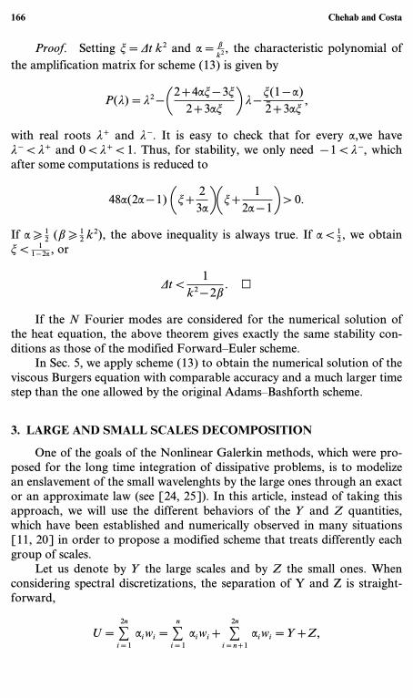
Proof. Setting t=Dt k2 and a= b

k2 , the characteristic polynomial ofthe amplification matrix for scheme (13) is given by

P(l)=l2 −12+4at − 3t

2+3at2 l −

t(1 − a)2+3at

,

with real roots l+ and l−. It is easy to check that for every a,we havel− < l+ and 0 < l+ < 1. Thus, for stability, we only need − 1 < l−, whichafter some computations is reduced to

48a(2a − 1) 1t+2

3a21t+

12a − 1

2 > 0.

If a \ 12 (b \ 1

2 k2), the above inequality is always true. If a < 12 , we obtain

t < 11 − 2a , or

Dt <1

k2 − 2b. i

If the N Fourier modes are considered for the numerical solution ofthe heat equation, the above theorem gives exactly the same stability con-ditions as those of the modified Forward–Euler scheme.

In Sec. 5, we apply scheme (13) to obtain the numerical solution of theviscous Burgers equation with comparable accuracy and a much larger timestep than the one allowed by the original Adams–Bashforth scheme.

3. LARGE AND SMALL SCALES DECOMPOSITION

One of the goals of the Nonlinear Galerkin methods, which were pro-posed for the long time integration of dissipative problems, is to modelizean enslavement of the small wavelenghts by the large ones through an exactor an approximate law (see [24, 25]). In this article, instead of taking thisapproach, we will use the different behaviors of the Y and Z quantities,which have been established and numerically observed in many situations[11, 20] in order to propose a modified scheme that treats differently eachgroup of scales.

Let us denote by Y the large scales and by Z the small ones. Whenconsidering spectral discretizations, the separation of Y and Z is straight-forward,

U= C2n

i=1aiwi= C

n

i=1aiwi+ C

2n

i=n+1aiwi=Y+Z,


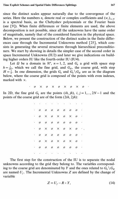
since the distinct scales appear naturally due to the convergence of theseries. Here the numbers ai denote real or complex coefficients and (wi)i ¥ N

is a spectral basis, as the Chebyshev polynomials or the Fourier basis(see [9]). When finite differences or finite elements are used, the abovedecomposition is not possible, since all the unknowns have the same orderof magnitude, namely that of the considered function in the physical space.Below, we present the construction of the distinct scales in the finite differ-ences case through the Incremental Unknowns method [25], which con-sists in generating the several structures through hierarchical preconditio-ners. We start by showing in details the simpler case of the second order inspace Incremental Unknowns (IU2) and later we give indications on build-ing higher orders IU like the fourth-order IU (IU4).

Let W be a domain in Rn, n=1, 2, and Gh a grid with space steph= 1

2N , which we call the fine grid, and GH, the coarse grid, with stepH= 1

N . In one dimension, the grids Gh and Gh 0GH are as in the diagrambelow, where the coarse grid is composed of the points with even indexes,marked with ×.

· o × o × o × o × o ·

In 2D, the fine grid Gh are the points (ih, jh), i, j=1,..., 2N − 1 and thepoints of the coarse grid are of the form (2ih, 2jh):

· · · · · · · · ·

· o o o o o o o ·

· o × o × o × o ·

· o o o o o o o ·

· o × o × o × o ·

· o o o o o o o ·

· o × o × o × o ·

· o o o o o o o ·

· · · · · · · · ·

.

The first step for the construction of the IU is to separate the nodalunknowns according to the grid they belong to. The variables correspond-ing to the coarse grid are denominated by Y and the ones related to Gh 0GH

are named Uf. The Incremental Unknowns Z are defined by the change ofvariable

Z=Uf − R p Y, (14)


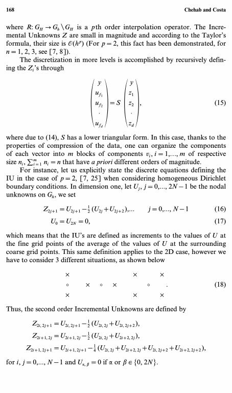
where R: GH Q Gh 0GH is a pth order interpolation operator. The Incre-mental Unknowns Z are small in magnitude and according to the Taylor’sformula, their size is O(hp) (For p=2, this fact has been demonstrated, forn=1, 2, 3, see [7, 8]).

The discretization in more levels is accomplished by recursively defin-ing the Zi’s through

Ry

uf1

uf2

·ufd

S=S Ryz1

z2

·zd

S , (15)

where due to (14), S has a lower triangular form. In this case, thanks to theproperties of compression of the data, one can organize the componentsof each vector into m blocks of components vi, i=1,..., m of respectivesize ni, ;m

i=1 ni=n that have a priori different orders of magnitude.For instance, let us explicitly state the discrete equations defining the

IU in the case of p=2, [7, 25] when considering homogeneous Dirichletboundary conditions. In dimension one, let Uj, j=0,..., 2N − 1 be the nodalunknowns on Gh, we set

Z2j+1=U2j+1 − 12 (U2j+U2j+2),... j=0,..., N − 1 (16)

U0=U2N=0, (17)

which means that the IU’s are defined as increments to the values of U atthe fine grid points of the average of the values of U at the surroundingcoarse grid points. This same definition applies to the 2D case, however wehave to consider 3 different situations, as shown below

× × ×p × p × p

× × ×. (18)

Thus, the second order Incremental Unknowns are defined by

Z2i, 2j+1=U2i, 2j+1 − 12 (U2i, 2j+U2i, 2j+2),

Z2i+1, 2j=U2i+1, 2j − 12 (U2i, 2j+U2i+2, 2j),

Z2i+1, 2j+1=U2i+1, 2j+1 − 14 (U2i, 2j+U2i+2, 2j+U2i, 2j+2+U2i+2, 2j+2),

for i, j=0,..., N − 1 and Ua, b=0 if a or b ¥ {0, 2N}.


The construction of higher order IUs is done through compactschemes. These schemes of compact stencil allow to obtain a level ofaccuracy comparable to the spectral one when discretizing differentialoperators [17]. They also generalize midpoint-like interpolation and areused in the definition of the higher order interpolation operator. Forinstance, in space dimension 1 (see also [5] for space dimensions two andthree) the interpolation operator matrix R, which is not explicit in this case,is defined as

R=P−1Q

where P and Q are respectively the N × N and the N × (N − 1) matrices

P=R1 1

6 0 · · 016 1 1

6 0 · ·0 1

6 1 16 · ·

· · · · · 0· · 0 1

6 1 16

0 · · 0 16 1

S , Q=R9996 − 21

96596 0 · 0

23

23 0 · · ·

0 23

23 0 · ·

· · · · · 0· · · 0 2

323

0 · · 596 − 21

969996

S .

In Fig. 1 below, we make a comparison between second and fourthorder IU’s, showing the higher degree of hierarchization accomplished bythis last one. We consider the function f(x)=sin(90x(1 − x)) sin(e3x),which exhibits many oscillations and gradients. We have used 511 points inthe discretization; the coarse grid is composed of 7 points and 7 grid levelswere used.

4. STABILITY ANALYSIS (LINEAR CASE)

In this section we demonstrate the enhanced stability properties of theresulting scheme after the conjunction of the temporal integration tech-niques of Sec. 2 and the Incremental Unknowns spatial discretization. Dis-tinctly from the spectral discretization, Finite Differences splittings are notable to make a complete separation of scales. Thus, high frequencies com-ponents are still present on the large scales provided by the IU discretiza-tion. This implies that the resulting time step restriction will be interme-diary between the one provided by the full grid and the one of the coarsegrid alone. Nevertheless, the gain in computation costs is apparent andclearly motivates the utilization of the splittings.

Below, we consider scheme (11) applied to the numerical solution ofthe 1d-heat equation. In order to show the weakening of the time step


0 0.2 0.4 0.6 0.8 1–15

–10

–5

0

5

10

15f(x)

x

f(x)

0 2 4 6 810

– 4

10–2

100

102

Norm of IU2 (+) and IU4 (v) components

grid level

Euc

lidia

n no

rm (

log1

0. s

cale

)

0 0.2 0.4 0.6 0.8 1–10

–5

0

5

10

15

20Function vs grid points in IU2 basis

x

S –

1 f

0 0.2 0.4 0.6 0.8 1–15

–10

–5

0

5

10

15

20Function vs grid points in IU4 basis

x

S–

1 f

(a) (b)

(c) (d)

Fig. 1. Hierarchization of the scales with IU2 and IU4. (a) the function f(x)=sin(90x(1 − x)) sin(e3x), (b) IU2 and IU4 components norm vs. grid level, (c) IU2 at gridpoints, (d) IU4 at grid points.

restriction, we perform an eigenvalues analysis of the resulting iterationmatrix. With the usual notations we have after the introduction of theincremental unknowns:

Rym+1

zm+1S=Rym

zmS− Dt

1h2R Id 0

01

1+b DtIdS S−1AS R

ym

zmS , (19)

h being the stepsize. Setting a= 11+b Dt , the study of the stability of scheme

(11) is reduced to the study of the spectral radius r(M) of the block-matrixM given by:

M=R Ac, c Ac, f

aAf, c aAf, f

S ,


where the submatrices Ai, j form the block decomposition of the IU discre-tization S−1AS and the stability condition is given by

0 < Dt <2h2

r(M).

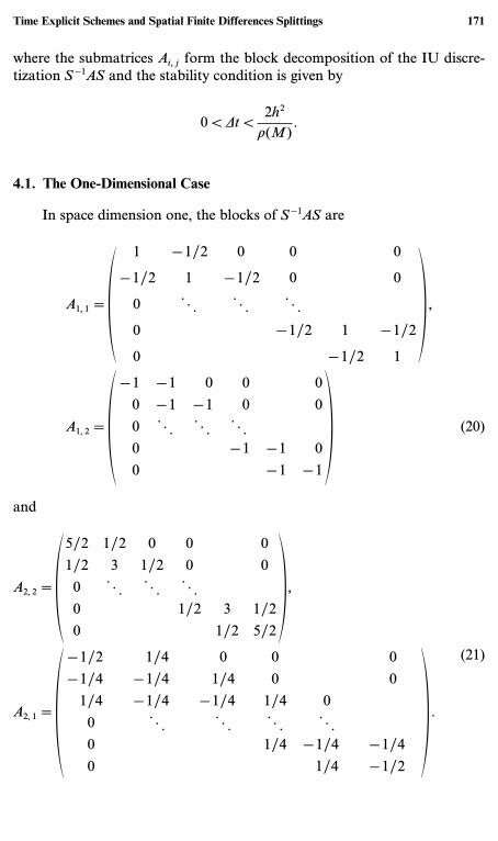
4.1. The One-Dimensional Case

In space dimension one, the blocks of S−1AS are

A1, 1=R1 − 1/2 0 0 0

− 1/2 1 − 1/2 0 0

0 z z z

0 − 1/2 1 − 1/2

0 − 1/2 1

S ,

A1, 2=R − 1 − 1 0 0 00 − 1 − 1 0 00 z z z

0 − 1 − 1 00 − 1 − 1

S (20)

and

A2, 2=R5/2 1/2 0 0 01/2 3 1/2 0 0

0 z z z

0 1/2 3 1/20 1/2 5/2

S ,

A2, 1=R− 1/2 1/4 0 0 0− 1/4 − 1/4 1/4 0 0

1/4 − 1/4 − 1/4 1/4 00 z z z z

0 1/4 − 1/4 − 1/40 1/4 − 1/2

S .

(21)


We consider 2N − 1 discretization points on the finest grid and wedenote the spatial stepsize by h= 1

2N , the computation domain being [0, 1].We have the following results

Lemma 4.1. The eigenvectors of A are given by

wp=Rsin(2pph)

sin(4pph)

x

sin((2N − 2) pph)

– – – –

sin(pph)

sin(3pph)

x

sin((2N − 1) pph)

S=R wp2i

– – – –wp

2i+1

S

for p=1,..., 2N − 1, with lp=2(1 − cos(pph)) as the associated eigen-values. The eigenvectors of S−1AS are

wp=Rsin(2pph)

sin(4pph)

x

sin((2N − 2) pph)

— −

sin(pph)(1 − cos(pph))

sin(3pph)(1 − cos(pph))

x

sin((2N − 1) pph)(1 − cos(pph))

S=R wp

2i

– – – –wp

2i+1(1 − cos(pph))

S=R wp2i

– – – –fp

2i+1

S .

Proof. The proof is straightforward by using the well known form ofthe eigenvalues and eigenvectors of tridiagonal matrices. i


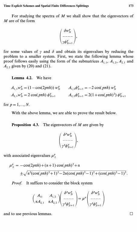
For studying the spectra of M we shall show that the eigenvectors ofM are of the form

R dwp2i

– – – –cfp

2i+1

S ,

for some values of c and d and obtain its eigenvalues by reducing theproblem to a smaller system. First, we state the following lemma whoseproof follows easily using the form of the submatrices A1, 1, A1, 2, A2, 1 andA2, 2 given by (20) and (21).

Lemma 4.2. We have

A1, 1wp2i=(1 − cos(2pph)) wp

2i A1, 2fp2i+1=−2 cos(pph) wp

2i

A2, 1wp2i=2 cos(pph) fp

2i+1 A2, 2fp2i+1=2(1+cos(pph)2) fp

2i+1

for p=1,..., N.

With the above lemma, we are able to prove the result below.

Proposition 4.3. The eigenvectors of M are given by

R dpwp2i

– – – –cpfp

2i+1

S ,

with associated eigenvalues mp±

mp± = − cos(2pph)+(a+1) cos(pph)2+a

± `a2(cos(pph)2+1)2 − 2a(cos(pph)2 − 1)2+(cos(pph)2 − 1)2 .

Proof. It suffices to consider the block system

R A11 A1, 2

aA2, 1 aA2, 2

SR dpwp2i

– – – –cpfp

2i+1

S=mp R dpwp2i

– – – –cpfp

2i+1

S

and to use previous lemmas. i


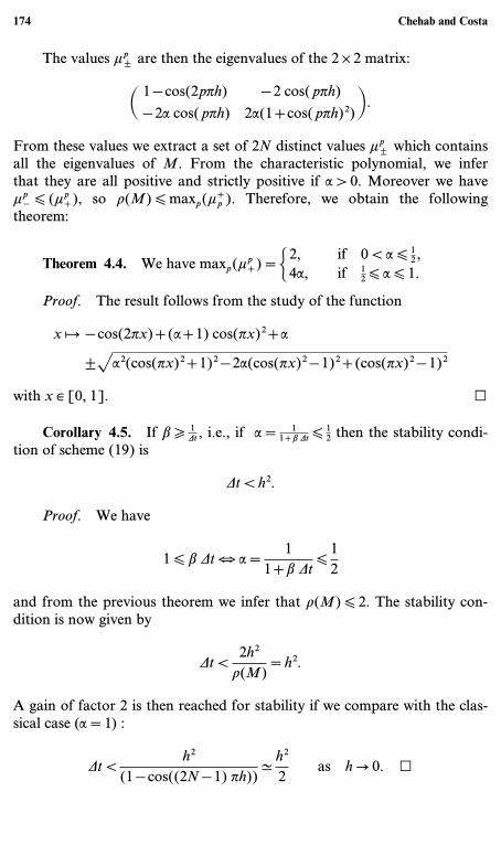
The values mp± are then the eigenvalues of the 2 × 2 matrix:

R 1 − cos(2pph) − 2 cos(pph)− 2a cos(pph) 2a(1+cos(pph)2)

S .

From these values we extract a set of 2N distinct values mp± which contains

all the eigenvalues of M. From the characteristic polynomial, we inferthat they are all positive and strictly positive if a > 0. Moreover we havemp

− [ (mp+), so r(M) [ maxp(m+

p ). Therefore, we obtain the followingtheorem:

Theorem 4.4. We have maxp(mp+)=˛2, if 0 < a [ 1

2 ,4a, if 1

2 [ a [ 1.

Proof. The result follows from the study of the function

x W − cos(2px)+(a+1) cos(px)2+a

± `a2(cos(px)2+1)2 − 2a(cos(px)2 − 1)2+(cos(px)2 − 1)2

with x ¥ [0, 1]. i

Corollary 4.5. If b \ 1Dt , i.e., if a= 1

1+b Dt [ 12 then the stability condi-

tion of scheme (19) is

Dt < h2.

Proof. We have

1 [ b Dt . a=1

1+b Dt[

12

and from the previous theorem we infer that r(M) [ 2. The stability con-dition is now given by

Dt <2h2

r(M)=h2.

A gain of factor 2 is then reached for stability if we compare with the clas-sical case (a=1) :

Dt <h2

(1 − cos((2N − 1) ph))4

h2

2as h Q 0. i


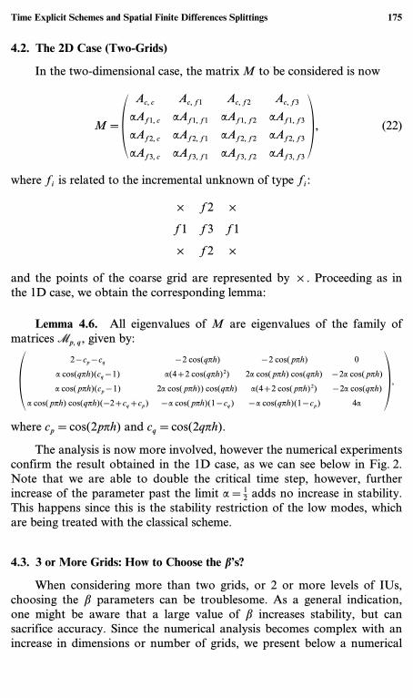
4.2. The 2D Case (Two-Grids)

In the two-dimensional case, the matrix M to be considered is now

M=RAc, c Ac, f1 Ac, f2 Ac, f3

aAf1, c aAf1, f1 aAf1, f2 aAf1, f3



S , (22)

where fi is related to the incremental unknown of type fi:

× f2 ×

f1 f3 f1

× f2 ×

and the points of the coarse grid are represented by × . Proceeding as inthe 1D case, we obtain the corresponding lemma:

Lemma 4.6. All eigenvalues of M are eigenvalues of the family ofmatrices Mp, q, given by:

R 2 − cp − cq − 2 cos(qph) − 2 cos(pph) 0

a cos(qph)(cq − 1) a(4+2 cos(qph)2) 2a cos(pph) cos(qph) − 2a cos(pph)

a cos(pph)(cp − 1) 2a cos(pph)) cos(qph) a(4+2 cos(pph)2) − 2a cos(qph)

a cos(pph) cos(qph)(−2+cq+cp) − a cos(pph)(1 − cq) − a cos(qph)(1 − cp) 4a

S ,

where cp=cos(2pph) and cq=cos(2qph).

The analysis is now more involved, however the numerical experimentsconfirm the result obtained in the 1D case, as we can see below in Fig. 2.Note that we are able to double the critical time step, however, furtherincrease of the parameter past the limit a=1

2 adds no increase in stability.This happens since this is the stability restriction of the low modes, whichare being treated with the classical scheme.

4.3. 3 or More Grids: How to Choose the b’s?

When considering more than two grids, or 2 or more levels of IUs,choosing the b parameters can be troublesome. As a general indication,one might be aware that a large value of b increases stability, but cansacrifice accuracy. Since the numerical analysis becomes complex with anincrease in dimensions or number of grids, we present below a numerical


0 1 2 30

0.5

1

1.5

2Spectral radius vs time step, alpha=0

dt/dtc

Spe

ctra

l rad

ius

0 1 2 30

0.5

1

1.5

2Spectral radius vs time step, alpha=0.5

dt/dtc

Spe

ctra

l rad

ius

0 1 2 30

1

2

3

4

5Spectral radius vs time step, alpha=0.75

dt/dtc

Spe

ctra

l rad

ius

0 1 2 30

1

2

3

4

5Spectral radius vs time step, alpha=1 (classical scheme)

dt/dtc

Spe

ctra

l rad

ius

Fig. 2. Spectral radius of the iteration matrix (2D case) vs. DtDtc

, for different values of a= 11+bDt .

study of the behavior of the spectral radius r(M), in the 2D case, forvarious numbers of IU levels and choices of b −s.

At first, we consider a two-dimensional mesh with 4 grids and 3 levelsof IUs, structured with 9 points per dimension in the coarse grid, totalling31 points in each direction. We set Dtc=

2h2

r(A) , the critical parameter of theclassical Euler scheme. The parameter b3 is always chosen as in Corollary 7above, i.e., b3= 1

Dtc. The remaining parameters are chosen as a geometric

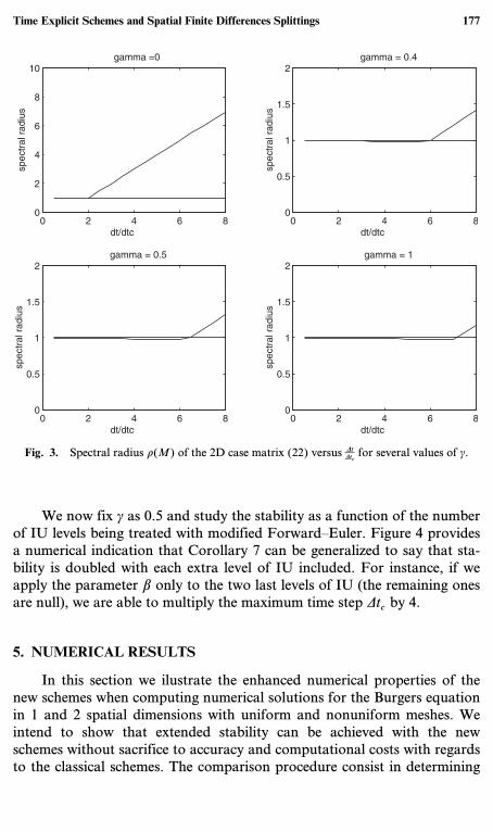
sequence through a multiplying factor c: bi=cbi+1. In Fig. 3 we plot thespectral radius r(M) as a function of the maximum time step for severalvalues of c. In the first graph, c=0 means that only the uppermost levelparameter is not null, i.e., only b3 is not zero. Note that in this case werecover the two grids case result when the maximum time step is doubled.Substantious extra stability is obtained up to a value of c=0.5; after that,increasing in stability slows, approaching the limit of 2Nl, where Nl is thenumber of IU levels.


0 2 4 6 80

2

4

6

8

10gamma =0

dt/dtc

spec

tral

rad

ius

0 2 4 6 80

0.5

1

1.5

2gamma = 0.4

dt/dtc

spec

tral

rad

ius

0 2 4 6 80

0.5

1

1.5

2gamma = 0.5

dt/dtc

spec

tral

rad

ius

0 2 4 6 80

0.5

1

1.5

2gamma = 1

dt/dtc

spec

tral

rad

ius

Fig. 3. Spectral radius r(M) of the 2D case matrix (22) versus DtDtc

for several values of c.

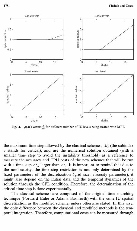
We now fix c as 0.5 and study the stability as a function of the numberof IU levels being treated with modified Forward–Euler. Figure 4 providesa numerical indication that Corollary 7 can be generalized to say that sta-bility is doubled with each extra level of IU included. For instance, if weapply the parameter b only to the two last levels of IU (the remaining onesare null), we are able to multiply the maximum time step Dtc by 4.

5. NUMERICAL RESULTS

In this section we ilustrate the enhanced numerical properties of thenew schemes when computing numerical solutions for the Burgers equationin 1 and 2 spatial dimensions with uniform and nonuniform meshes. Weintend to show that extended stability can be achieved with the newschemes without sacrifice to accuracy and computational costs with regardsto the classical schemes. The comparison procedure consist in determining


0 5 10 150

0.5

1

1.5

24 last levels

dt/dtc

spec

tral

rad

ius

0 5 10 150

1

2

3

43 last levels

dt/dtc

spec

tral

rad

ius

0 5 10 150

2

4

6

82 last levels

dt/dtc

spec

tral

rad

ius

0 5 10 150

5

10

15

last level

dt/dtc

spec

tral

rad

ius

Fig. 4. r(M) versus DtDtc

for different number of IU levels being treated with MFE.

the maximum time step allowed by the classical schemes, Dtc (the subindexc stands for critical), and use the numerical solution obtained (with asmaller time step to avoid the instability threshold) as a reference tomeasure the accuracy and CPU costs of the new schemes that will be runwith a time step Dtm larger than Dtc. It is important to remind that due tothe nonlinearity, the time step restriction is not only determined by thefixed parameters of the discretization (grid size, viscosity parameter); itmight also depend on the initial data and the temporal dynamics of thesolution through the CFL condition. Therefore, the determination of thecritical time step is done experimentally.

The classical schemes are composed of the original time marchingtechnique (Forward–Euler or Adams–Bashforth) with the same IU spatialdiscretization as the modified scheme, unless otherwise stated. In this way,the only difference between the classical and modified methods is the tem-poral integration. Therefore, computational costs can be measured through


number of iterations, since the modifications in the time scheme incurs inno relevant extra number of operations. Nevertheless, in the last examplewe make a full comparison between a one grid spatial discretization (noIncremental Unknowns) with the classical temporal scheme and theconjugated scheme here proposed.

5.1. 1D Burgers Equation

We start by computing the steady-state solution of the 1-D viscousBurgers equation with Dirichlet boundary conditions

“u“t

− n“

2u“x2+u

“u“x

=f in ]0, 1[, t > 0,

u(x, 0)=u0(x),

u(0, t)=u(1, t)=0, -t > 0,

(23)

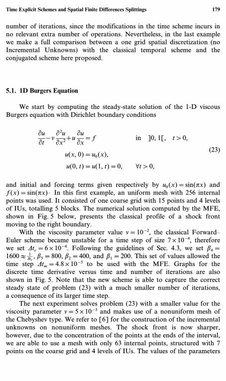
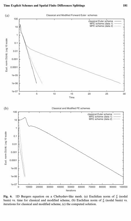
and initial and forcing terms given respectively by u0(x)=sin(px) andf(x)=sin(px) · In this first example, an uniform mesh with 256 internalpoints was used. It consisted of one coarse grid with 15 points and 4 levelsof IUs, totalling 5 blocks. The numerical solution computed by the MFE,shown in Fig. 5 below, presents the classical profile of a shock frontmoving to the right boundary.

With the viscosity parameter value n=10−2, the classical Forward–Euler scheme became unstable for a time step of size 7 × 10−4, thereforewe set Dtc=6 × 10−4. Following the guidelines of Sec. 4.3, we set b4=1600 % 1

Dtc, b3=800, b2=400, and b1=200. This set of values allowed the

time step Dtm=4.8 × 10−3 to be used with the MFE. Graphs for thediscrete time derivative versus time and number of iterations are alsoshown in Fig. 5. Note that the new scheme is able to capture the correctsteady state of problem (23) with a much smaller number of iterations,a consequence of its larger time step.

The next experiment solves problem (23) with a smaller value for theviscosity parameter n=5 × 10−3 and makes use of a nonuniform mesh ofthe Chebyshev type. We refer to [6] for the construction of the incrementalunknowns on nonuniform meshes. The shock front is now sharper,however, due to the concentration of the points at the ends of the interval,we are able to use a mesh with only 63 internal points, structured with 7points on the coarse grid and 4 levels of IUs. The values of the parameters


0 2 4 610

–10

10–5

100

105

IdU/dtI vs time

time

IdU

/dtI

0 2000 4000 6000 8000 1000010

–10

10–5

100

105

IdU/dtI vs iterations

iterations

IdU

/dtI

0 0.1 0.2 0.3 0.4 0.5 0.6 0.7 0.8 0.9 10

0.2

0.4

0.6

0.8

1

1.2

1.4MFE solution

x

U

(a) (b)

(c)

Fig. 5. 1D Burgers equation on a uniform mesh. (a) Euclidian norm of ddt (nodal basis) vs.

time for classical and extended scheme, (b) Euclidian norm of ddt (nodal basis) vs. iterations for

classical and extended scheme, (c) the computed solution.

b −s are again dictated by the maximum time step allowed by the classicalFE which is Dtc=5 × 10−5. This determines b4=17000 % 1

Dtc. However,

smaller values for the remaining b −s suffice to allow Dtm=10−3: b3=500,b2=50, and b1=5. This is due to the fact that the Chebyshev mesh is ableto concentrate the stability restrictive high gradients of the shock profile inits uppermost level, i.e., it performs a more stronger scales separation thanthe uniform mesh. As we can see in Fig. 6 the gain in CPU costs are morethan tenfold with a little change in the accuracy of the dynamics. A thirdcase is also shown in Fig. 6, which correspond to a bigger value ofb4=20000. Note that computational costs are smaller, due to the increaseon the time step to Dt −

m=5 × 10−3, however accuracy in time is affected,showing that a compromise must be reached between extra stability andprecision. A clear illustration of this fact will be shown below in the 2Dcase.


1e-07

1e-06

1e-05

0.0001

0.001

0.01

0.1

1

10

100

0 5 10 15 20 25 30

Euc

l. no

rm D

U/d

t, Lo

g.10

sca

le

Time

Classical and Modified Forward Euler schemes

classical Euler schemeMFE scheme (data 1)MFE scheme (data 2)

(a)

1e-07

1e-06

1e-05

0.0001

0.001

0.01

0.1

1

10

100

0 10000 20000 30000 40000 50000 60000 70000 80000 90000 100000

Euc

l. no

rm D

U/d

t, Lo

g.10

sca

le

Iterations

Classical and Modified FE schemes

classical Euler schemeMFE scheme (data 1)MFE scheme (data 2)

(b)

Fig. 6. 1D Burgers equation on a Chebyshev-like mesh. (a) Euclidian norm of ddt (nodal

basis) vs. time for classical and modified scheme, (b) Euclidian norm of ddt (nodal basis) vs.

iterations for classical and modified scheme, (c) the computed solution.


0

0.2

0.4

0.6

0.8

1

1.2

0 0.1 0.2 0.3 0.4 0.5 0.6 0.7 0.8 0.9 1

u

x

MFE computed solution, nu=0.005, Chebyshev mesh (63 pts)

solution

(c)

Fig. 6. (Continued).

5.2. Comparison to Semi-Implicit Schemes

We now compare the modified second order Adams–Bashforth scheme(MAB2) of Sec. 2 to the semi-implicit discretization provided by theCrank–Nicolson scheme applied to the linear term and Adams–Bashforthto the nonlinear one (CNAB2). We have also included the original secondorder Adams–Bashforth in order to make more explicit the distinct behav-ior of the modified scheme. The spatial discretization is carried out in allschemes above by the fourth-order compact schemes ([17]) which makesthe temporal error the dominant one.

Problem (23) is solved with n=10−2 and the exact solution u(x, t)=sin[10x(1 − x)(sin pt+2)], which exhibits a fast variation in time. Themesh is composed of a coarse grid with 7 points and 4 levels of IUs, totall-ing 127 internal points. The maximum allowed time step for the classicalAB2 is Dtc=9 × 10−4, setting the following value for the parameters to beused in the MAB2 scheme:

b4=1111, b3=111, b2=11.11, and b1=1.111.


0 2 4 6 8 10 12 14 1610

–5

10– 4

10– 3

10–2

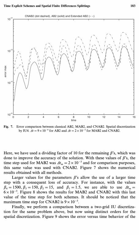
CNAB2 (dot dashed), AB2 (solid) and Extended AB2 (– –)

time

erro

r m

ax

Fig. 7. Error comparison between classical AB2, MAB2, and CNAB2. Spatial discretizationby IU4. Dt=9 × 10−4 for AB2 and Dt=2 × 10−3 for MAB2 and CNAB2.

Here, we have used a dividing factor of 10 for the remaining b −s, which wasdone to improve the accuracy of the solution. With these values of b −s, thetime step used for MAB2 was Dtm=2 × 10−3 and for comparison purposes,this same value was used with CNAB2. Figure 7 shows the numericalresults obtained with all methods.

Larger values for the parameters b −s allow the use of a larger timestep with a consequent loss of accuracy. For instance, with the valuesb4=1500, b3=150, b2=15, and b1=1.5, we are able to use Dtm=6 × 10−3. Figure 8 shows the results for MAB2 and CNAB2 with this lastvalue of the time step for both schemes. It should be noticed that themaximum time step for CNAB2 is 9 × 10−3.

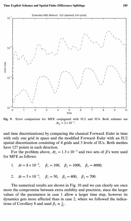
Finally, we perform a comparison between a two-grid IU discretiza-tion for the same problem above, but now using distinct orders for thespatial discretization. Figure 9 shows the error versus time behavior of the


0 5 10 1510

–4

10– 3

10– 2

10–1

CNAB2 (dashed) and Extended AB2 (solid)

time

erro

r m

ax

Fig. 8. Error comparison for MAB2 and CNAB2. Spatial discretization by IU4.Dt=6 × 10−3.

modified temporal schemes conjugated with the second and fourth ordersIUs. The value of the parameter b1=1110 is the same for both schemes.

5.3. 2D Case

We now consider the 2D scalar Burgers-like equation:

ut −1

ReDu+u div (u)=f in W=]0, 1[2,

u(. , t)=g on “W, t > 0,

u(x, y, 0)=u0(x, y),

(24)

with n=5 × 10−2 and exact solution given by u(x, y, t)=(2 − e4 sin t

1+10t2). In thisexample, we test the new schemes against the full classical method (spatial


0 1 2 3 4 5 6 7 8 9 1010

–4

10–3

10–2

10–1

Extended AB2 Method : IU2 (dashed) IU4 (solid)

time

erro

r m

ax

Fig. 9. Error comparison for MFE conjugated with IU2 and IU4. Both schemes useDtm=2 × 10−3.

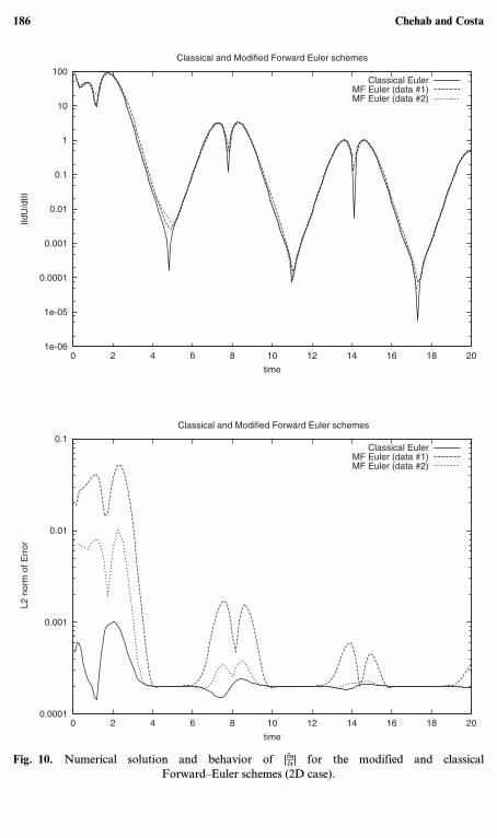
and time discretizations) by comparing the classical Forward–Euler in timewith only one grid in space and the modified Forward–Euler with an IU2spatial discretization consisting of 4 grids and 3 levels of IUs. Both mesheshave 127 points in each direction.

For the problem above, Dtc=1.3 × 10−3 and two sets of b −s were usedfor MFE as follows:

1. Dt=8 × 10−3, b1=100, b2=1000, b3=4000;

2. Dt=5 × 10−3, b1=50, b2=400, b3=700.

The numerical results are shown in Fig. 10 and we can clearly see oncemore the compromise between extra stability and precision, since the largervalues of the parameters in case 1 allow a larger time step, however itsdynamics gets more affected than in case 2, where we followed the indica-tions of Corollary 8 and used b3 % 1

Dtc.


1e-06

1e-05

0.0001

0.001

0.01

0.1

1

10

100

0 2 4 6 8 10 12 14 16 18 20

IIdU

/dtII

time


Classical EulerMF Euler (data #1)MF Euler (data #2)

0.0001

0.001

0.01

0.1

0 2 4 6 8 10 12 14 16 18 20

L2

norm

of E

rror

time



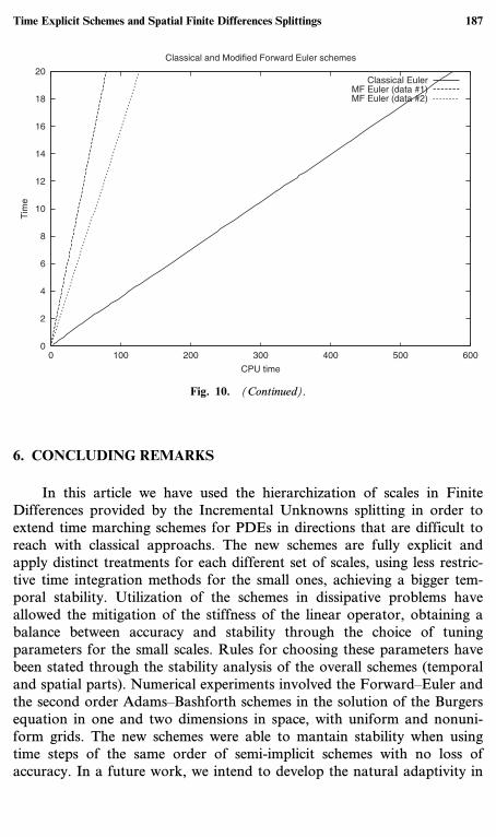
Fig. 10. Numerical solution and behavior of |“u“t| for the modified and classical

Forward–Euler schemes (2D case).


0

2

4

6

8

10

12

14

16

18

20

0 100 200 300 400 500 600

Tim

e

CPU time



Fig. 10. (Continued).

6. CONCLUDING REMARKS

In this article we have used the hierarchization of scales in FiniteDifferences provided by the Incremental Unknowns splitting in order toextend time marching schemes for PDEs in directions that are difficult toreach with classical approachs. The new schemes are fully explicit andapply distinct treatments for each different set of scales, using less restric-tive time integration methods for the small ones, achieving a bigger tem-poral stability. Utilization of the schemes in dissipative problems haveallowed the mitigation of the stiffness of the linear operator, obtaining abalance between accuracy and stability through the choice of tuningparameters for the small scales. Rules for choosing these parameters havebeen stated through the stability analysis of the overall schemes (temporaland spatial parts). Numerical experiments involved the Forward–Euler andthe second order Adams–Bashforth schemes in the solution of the Burgersequation in one and two dimensions in space, with uniform and nonuni-form grids. The new schemes were able to mantain stability when usingtime steps of the same order of semi-implicit schemes with no loss ofaccuracy. In a future work, we intend to develop the natural adaptivity in


time and space provided by the separation of scales and the use of the sta-bility parameters in order to reduce computational costs for the numericalsolution of the incompressible Navier–Stokes equation and simulation ofits related physical phenomena.

ACKNOWLEDGMENTS

Part of this work was done while the first author was visiting theInstituto de Matemática—UFRJ, Rio de Janeiro. The second author waspartly supported by CNPQ Grant 300-315/98-8 and by FAPERJ GrantE-26/170.216/2000.

REFERENCES

1. Ascher, U., and Petzold, L. (1998). Computer Methods for Ordinary Differential Equationsand Differential-Algebraic Equations, SIAM.

2. Calgaro, C., Laminie, J., and Temam, R. (1997). Dynamical multilevel schemes for thesolution of evolution equations by hierarchical finite element discretization. Appl. Num.Math. 23, 403–442.

3. Chehab, J.-P., and Temam, R. (1995). Incremental unknowns for solving nonlineareigenvalue problems: New multiresolution methods. Numer. Methods Partial DifferentialEquations 11, 199–228.

4. Chehab, J.-P. (1996). Solution of generalized Stokes problems using hierarchical methodsand incremental unknowns. Appl. Numer. Math. 21, 9–42.

5. Chehab, J.-P. (1998). Incremental unknowns method and compact schemes. M2AN 32 (1),51–83.

6. Chehab, J.-P., and Miranville, A. (1998). Incremental unkowns method on nonuniformmeshes. M2AN 32 (5), 539–577.

7. Chen, M., and Temam, R. (1991). Incremental unknowns for solving partial differentialequations. Numer. Math. 59, 255–271.

8. Chen, M., Miranville, A., and Temam, R. (1995). Incremental unknowns in finite differ-ence in three space dimension. Comput. Appl. Math. 14 (3), 1–15.

9. Costa, B, and Dettori, L. (1998). Fourier collocation splittings for partial differentialequations, J. Comput. Phys. 20, 469–475.

10. Costa, B., Dettori, L., Gottlieb, D., and Temam, R. (2001). Time marching techniques forthe nonlinear Galerkin method. SIAM. J. SC. Comp. 23 (1), 46–65.

11. Debussche, A., Dubois, T., and Temam, R. (1995). The nonlinear Galerkin method:A multiscale method applied to the simulation of homogeneous turbulent flows, andtheoretical and computational fluid dynamics 7 (4), 279–315.

12. Dettori, L., Gottlieb, D., and Temam, R. (1995). A nonlinear Galerkin method: The two-level Fourier-collocation case. J. Sci. Comput. 10 (4), 371–389.

13. Dettori, L., Gottlieb, D., and Temam R. (1996). A nonlinear Galerkin method: The two-level Chebyshev-collocation case. In Ilin, A. V., and Scot, L. R. (eds), Special Issue ofHouston Journal of Mathematics, pp. 75–83.

14. Dubois, T., Jauberteau, F., and Temam, R. (1999). Dynamic, Multilevel Methods and theNumerical Simulation of Turbulence, Cambridge University Press.


15. Fornberg, B., and Whitham, G. B. (1978). A numerical and theoretical study of certainnonlinear wave phenomena. Philos. Trans. Roy. Soc. London Ser. A 289, 373–404.

16. Goubet, O. (1992). Construction of approximate inertial manifolds using wavelets, SIAMJ. Math. Anal. 23 (6), 1455–1481.

17. Lele, S. K. (1992). Compact finite difference schemes with spectral-like resolution.J. Comput. Phys. 103, 16–42.

18. Jolly, M. S., Rosa, R., and Temam, R. Accurate computations on inertial manifolds.SIAM. J. Sci. Comput. 22 (6), 2216–2238.

19. Marion, M., and Temam, R. (1989). Nonlinear Galerkin methods: SIAM J. Numer. Anal.26, 1139–1157.

20. Marion, M., and Temam, R., (1990). Nonlinear Galerkin methods; The finite elementscase. Numer. Math. 57, 205–226.

21. Pouit, F. (décembre 1998). Thèse, Université Paris-Sud, Orsay.22. Simonnet, E. (décembre 1998). These, Université Paris-Sud.23. Tachim Medjo, T. (1997). Numerical solutions of the Navier–Stokes equations using

wavelet-like incremental unknowns. RAIRO Model. Math. Anal. Numér. 31 (7), 827–844.24. Temam, R. (1997). Infinite Dimensional Dynamical Systems in Mechanics and Physics,

Springer Verlag, Berlin, (2nd ed.).25. Temam, R. (1990). Inertial manifolds and multigrid methods. SIAM J. Math. Anal. 21,

154–178.


time explicit schemes and spatial finite differences ...bcosta/papers/fulltext.pdftime explicit...

Documents