a low communication and large time step explicit finite

A Low Communication and Large Time Step Explicit Finite-Volume Solver forNon-Hydrostatic Atmospheric Dynamics

Matthew R. Normana,∗, Ramachandran D. Nairb, Fredrick H. M. Semazzia

aDepartment of Marine, Earth, and Atmospheric Science, North Carolina State University, Raleigh, NC, USAbInstitute for Mathematics Applied to Geosciences, National Center for Atmospheric Research, Boulder, CO, USA

Abstract

An explicit finite-volume solver is proposed for numerical simulation of non-hydrostatic atmospheric dynamics withpromise for efficiency on massively parallel machines via low communication needs and large time steps. Solvingthe governing equations with a single stage lowers communication, and using the method of characteristics to fol-low information as it propagates enables large time steps. Using a non-oscillatory interpolant, the method is stablewithout post-hoc filtering. Characteristic variables (built from interface flux vectors) are integrated upstream frominterfaces along their trajectories to compute time-averaged fluxes over a time step. Thus we call this method an Flux-Based Characteristic Semi-Lagrangian (FBCSL) method. Multidimensionality is achieved via a second-order accurateStrang operator splitting. Spatial accuracy is achieved via the third- to fifth-order accurate Weighted Essentially Non-Oscillatory (WENO) interpolant.

We implement the theory to form a 2-D non-hydrostatic compressible (Euler system) atmospheric model in whichstandard test cases confirm accuracy and stability. We maintain stability with time steps larger than CFL=1 but notethat accuracy degrades unacceptably for most case with CFL >2. For the smoothest test case, we ran out to CFL=7 toinvestigate the error associated with simulation at large CFL time steps. Analysis suggests improvement of trajectorycomputations will improve error for large CFL numbers.

Key words: finite volume, atmospheric dynamics, non-hydrostatic, Riemann solver, fully discrete, flux vectorsplitting

1. Introduction

Inclusion of non-hydrostatic dynamics in atmospheric models has already become the norm for mesoscale andsynoptic scale models [32, 33] because of the resolved atmospheric features on non-hydrostatic scales. It is alsoquickly becoming a desirable feature of even global climatemodels to accommodate future multi-scale techniquessuch as adaptive grid refinement. Even quasi-uniform resolution global models are approaching grid spacings in thetens of kilometers [10] which means non-hydrostatic dynamics are an application of importance.

Efficient numerical integration of non-hydrostatic atmospheric dynamical equations is complex with large dis-tributed memory parallel machines in the picture. In the reign of Moore’s law (exponentially increasing single CPUcompute power), Semi-Implicit Semi-Lagrangian (SISL) methods provided excellent efficiency [34, 29, 6]. In thecurrent era of Massively Parallel Machines (MPMs) which distribute system memory among 10,000s of nodes, com-municating data between nodes is costly. High communication requirements of SISL methods force diminishingreturns before reaching the capacity of current machines. Therefore, these methods along with fully implicit methods[18, 13] have difficulty scaling current machines in Amdahl’s sense [3] with a reasonable problem size and throughput.

We take “scalable” to mean throughput scaling, closely related to Gustafson’s notion of weak scaling [16]. Sup-pose a method can simulate on a given grid at the rate of five Simulated Years Per Day (SYPD), a number generallyaccepted in the climate modeling community for future projections. If we refine the grid in half, that method scalesperfectly if it retains five SYPD by spreading the larger problem across 23 = 8 times more processors (for three spa-tial dimensions). Explicit methods cannot scale in this manner due to the Courant-Friedrichs-Lewy (CFL) condition

∗Corresponding authorEmail addresses:mrnormann su.edu (Matthew R. Norman),rnairu ar.edu (Ramachandran D. Nair),semazzin su.edu

(Fredrick H. M. Semazzi)

Preprint submitted to Jounrnal of Computational Physics April 23, 2010

2

which requires time step reduction with grid refinement. However, because explicit methods have low communicationneeds, they scale by Amdahl’s definition of taking a fixed problem size and spreading it among as many processors aspossible. Low-communication explicit methods have shown good utilization of MPMs and throughput at high reso-lutions for atmospheric flow [10]. Therefore, we explore here a new explicit method with a balance of time step andcommunication that we believe forms a competitive middle ground in terms of efficiency among existing methods.First, we review previous explicit methods used for atmospheric dynamics.

The most popular Finite-Volume (FV) methods for the atmosphere are central semi-discrete solvers [17, 9, 12, 14,23]. “Central” means there is no upwinding for the full dynamical equation set. The CFL of these methods is limitedgenerally to one (though moderately higher for some of the semi-discrete solvers). In particular, multi-stage solversrequire communication between each stage which can increase communication burden on MPMs. It is common to seethese methods coupled with split-explicit sub-cycling treatments which split the equation set into fast (sound waves /external gravity waves) and slow (transport) waves. Concerning communication, one could consider the sub-cyclingto be similar to multi-stage solvers in that communication is necessary in between each fast wave solve. However,sub-cycling enables significantly larger time steps with little additional computation which increases efficiency.

Upwind Godunov-type methods are another FV class [8, 1, 2]. For the atmosphere, they are an emerging appli-cation even though one was applied as far back as two decades ago [8]. Of particular interest to the present paper aremethods of this class which implement fully discrete time solvers (meaning one step, one stage) because they exhibitlow communication requirements in parallel. To a large extent, this schemes developed herein were motivated by thetheory and attributes of these types of methods. These all have CFL limitations of one, and high-order accuracy isobtained via Taylor series expansions limited with van Leertype limiters.

Galerkin methods [26, 11, 15, 20, 25] belong to the Finite Element class. They generally come in two flavors:Discontinuous Galerkin (DG) and Continuous Galerkin / Spectral Element (SE). They have differing CFL limitationsfor stability, but both time steps decrease as the order of accuracy increases as well as when grid spacing decreases.Because Galerkin methods use multiple degrees of freedom (either nodal or modal), they can perform high-orderaccurate reconstruction without communication leading toa very low communication burden. Non-oscillatory limitingof the spatial approximations within elements is an active area of research [5] which tends to add to the communicationburden. Even with time step limitations, because of the low communication requirements the spectral element methodhas already been shown to perform very well for atmospheric flows [37, 10].

Constrained interpolation profile (CIP) methods [22, 36, 38, 24, 21] are FV methods that also evolve point values(and derivatives) at cell boundaries to make reconstruction more local. CIP methods using characteristics [36, 21]have much in common with the method being presented here. Both compute interface fluxes by tracing characteristicvariables out from the interface using characteristic trajectories. Thus, they can simulate at large CFL numbers. Here,we use flux-based characteristic variables for easing the maintenance of hydrostatic balance, and we do not makethe assumption that the averaged flux vector is equal to the flux computed using averaged state variables (see section2.4.1). Additionally, we do not make use of cell interface point values, but we evolve only the cell means.

Here, we propose a new solver for atmospheric dynamics with the potential for competitive efficiency throughlow communication requirements (enabling better scaling on large parallel machines) and large time steps (improvingoverall efficiency). It is a high-order accurate, upwind, fully discrete, and non-oscillatory solver based on a flux vectorsplitting analog of f-waves [4, 19]. The flux vector splitting is what enables large time steps, and we extend our methodto large CFL numbers in this paper to determine and discuss the errors and complications involved with explicit largeCFL simulation. We call this method a Flux-Based Characteristic Semi-Lagrangian (FBCSL) method.

Given the scheme’s flexibility to accommodate any spatial interpolant, we use the third- to fifth-order accurateWeighted Essentially Non-Oscillatory (WENO) method as implemented in [7]. The WENO philosophy of [31] and[30] involves a weighted sum of polynomials where the least oscillatory polynomials are weighted the highest. Onecould also use, for instance, non-polynomial interpolantsas well ( [27, 28]). Three standard 2-D non-hydrostatic testcases will be performed to validate the proposed method. Themethod is described in section 2, validation throughnumerical simulation of non-hydrostatic test cases is given in section 3, and concluding remarks and future work aregiven in section 4.

2. Numerical Method

2.1. 2-D Compressible Non-Hydrostatic Equation Set

In this study, we use a two-dimensional, compressible, non-hydrostatic model (essentially the Euler system ofequations) which explicitly conserves mass, momentum, andpotential temperature (and therefore entropy). A Carte-

2.2 Fully Discrete FV Framework 3

sian rectangular grid is used for spatial discretization. The equation set is as follows:

∂U∂ t

+∂F(U)

∂x+

∂H(U)

∂z= S (1)

U =

ρρuρwρθ

, F(U) =

ρuρu2+ p

ρuwρuθ

, G(U) =

ρwρwu

ρw2 + pρwθ

, S(U) =

00

−ρg0

(2)

whereρ is the density,u is the horizontal wind,w is the vertical wind,p is the pressure, andθ is the potentialtemperature which is related to the actual temperature,T, by θ = T (p0/p)Rd/cp. The equation set is closed by the

equation of state:p = C0 (ρθ )γ where the constantC0 is defined by:C0 = Rγdp

−Rd/cp0 . The constants areγ = cp/cv ≈

1.4, Rd = 287 Jkg−1K−1, cp = 1004 Jkg−1K−1, cv = 717 Jkg−1K−1, andp0 = 105 Pa.

2.2. Fully Discrete FV FrameworkIn FV models, the spatial domain is spanned by cells, and the cell-averaged state variables are evolved between

them by fluxes through cell interfaces. To approximate the equations, the entire equation set is integrated over one ofthese computational cells with a domain ofΩi, j ∈

[xi−1/2, j ,xi+1/2, j

]×

[zi, j−1/2,zi, j+1/2

]wherexi±1/2, j = xi, j ±∆x/2

andzi, j±1/2 = zi, j ±∆z/2 refer to cell interface locations and∆x and∆z are the horizontal and vertical grid spacing,respectively. Next, the Gauss divergence theorem is applied to the flux divergence integrals, transforming them intoline integrals of the normal flux over the cell boundaries. Ona rectangular, Cartesian grid, this gives:

∂Ui, j

∂ t+

1∆x

[Fi+1/2, j (U)−Fi−1/2, j (U)

]+

1∆z

[Hi, j+1/2(U)−Hi, j−1/2(U)

]= Si, j (3)

The flux evaluations in time will be fully discrete, meaning the equations are integrated in time directly. Since anintegral is the product of the average and the interval of integration, this can be rewritten as:

Un+1i, j = U

ni, j −

∆t∆x

[Fi+1/2, j (U)− Fi−1/2, j (U)

]−

∆t∆z

[Hi, j+1/2(U)− Hi, j−1/2(U)

]+ ∆tSi, j (4)

where the hat above a variable denotes an average over the time step, a superscriptn denotes the variable valid at timen∆t, and∆t is the time step.

2.3. Strang Splitting: Multidimensionality & Source TermFinally, a second-order accurate Strang splitting is applied to integrate the fluxes in a sequence of 1-D sweeps.

Consider the following update operators on any given cell:

x(U

n)= U

ni, j −

∆t∆x

[Fi+1/2, j

(U

ni− s−1

2 , j , . . . ,Uni+ s+1

2 , j

)− Fi−1/2, j

(U

ni− s+1

2 , j , . . . ,Uni+ s−1

2 , j

)](5)

z(U

n)= U

ni, j −

∆t∆z

[(Hi, j+1/2

(U

ni, j− s−1

2, . . . ,U

ni, j+ s+1

2

)− Hi, j−1/2

(U

ni, j− s+1

2, . . . ,U

ni, j+ s−1

2

))](6)

S(U

n)= U

ni, j + ∆tSi, j

(U

ni, j

)(7)

wheres is the size of the stencil used for spatial reconstruction (see section 2.4.1). Our WENO approximation has avalues= 5. We introduce the stencil size in here to show that the flux computations only depend on a local set ofcells. The splitting procedure is implemented as follows for all cells i, j:

U∗i, j = x

(U

n)(8)

U∗∗i, j = z

(U∗)

Un+1i, j = S

(U∗∗

)

U∗i, j = S

(U

n+1)

U∗∗i, j = z

(U∗)

Un+2i, j = x

(U∗∗

)

2.4 Flux Evaluations 4

With the exception of the dimensional splitting and the source term, the accuracy depends entirely on the approxi-mation of the time-averaged interface fluxes.

2.4. Flux Evaluations

2.4.1. Flux-Based Characteristic Variables (CVs)The equation set given in 1 is classified as hyperbolic because after applying the chain rule to the fluxes, the

resulting matrix (see below), called the flux Jacobian, can be decomposed into eigenvalues and eigenvectors that areguaranteed to have real (non-imaginary) values. Put in characteristic form, the homogeneous equation set (consideringonly thex-direction for clarity) becomes:

∂U∂ t

+∂F∂U

∂U∂x

= 0 (9)

where∂F/∂U = A is the flux Jacobian matrix. From here, we must operate under the assumption of a “locallyfrozen” Jacobian to use linear characteristic theory. At each interface, the flux Jacobian is locally help constantin time and uniform in space during a time step, computed by state variables which are representative of the localspatiotemporal fluid environment. Once locally froze, the flux Jacobian can be diagonalized into eigenvectors andeigenvalues:A = RΛL whereR is a matrix whose columns are right eigenvectors,L is a matrix whose rows are lefteigenvectors,Λ is a diagonal matrix whose diagonal components are eigenvalues, andL = R−1. For the entropy-basedEuler equation set (1), the eigenvectors are (in thex- andz-directions):

Rx =

1 0 1 1

u 0 u−cs u+cs

0 1 w w

0 0 θ θ

, Rz =

0 1 1 1

1 0 u u

0 w w−cs w+cs

0 0 θ θ

(10)

Lx =

1 0 0 − 1θ

0 0 1 −wθ

u2cs

− 12cs

0 12θ

− u2cs

12cs

0 12θ

, Lz =

0 1 0 − uθ

1 0 0 − 1θ

w2cs

0 − 12cs

12θ

− w2cs

0 12cs

12θ

(11)

wherecs =√

γ p/ρ is the speed of sound. Also, the corresponding eigenvalues are: Λx = diag(u,u,u−cs,u+cs) andΛz = diag(w,w,w−cs,w+cs).

[19] shows that, for any hyperbolic equation set, the difference in the flux across an interface can be described asa weighted sum of the right eigenvectors:

F(Ui

)−F

(Ui−1

)≡ ∆Fi−1/2 = ∑

pβ p

i−1/2rpi−1/2 (12)

Throughout, a superscriptp is not an exponent but refers to one of the four characteristic waves admitted by thisequation set. A characteristic wave is defined by a right eigenvectorrp

i−1/2 (the p-th column ofR computed at an

interface), a left eigenvectorlpi−1/2 (the p-th row of L computed at the interface), and an eigenvalueλ p (the p-th

diagonal element ofΛ). The value,β pi−1/2, is a flux difference based CV calculated byβ p

i−1/2 = lpi−1/2 ·∆Fi−1/2. The

eigenvalues,λ p, define the velocities of the trajectories along which CVs are materially conserved. To compute theinterface eigenvectors,L andR, any value representative of the surroundings will suffice because the CVs are basedon the flux vector and not state variables (see [2, 4]). Also, Roe-averaging doesn’t exist yet for the equation set weare using. Therefore, we take a simple average of the surrounding state variables at the interface to constructL andR.

Alternatively, the flux vector itself at an interface (rather than the difference across an interface) can be describedas a weighted sum of the right eigenvectors, and this is the approach taken here. To obtain the flux through an interface

2.4 Flux Evaluations 5

at a given time, we need the flux vector based CVs arriving at the interface at that time:wpi−1/2(t) = lp

i−1/2 ·F(U,t).Then, the flux at a given time is:

Fi−1/2(t) = ∑p

wpi−1/2 (t)rp

i−1/2 (13)

Now, to obtain time-averaged fluxes, we need to integrate theCVs arriving at the interface over a time step, and thiswill be discussed in section 2.4.2.

Advantages of Flux-Based CVs.There are two main advantages to using flux-based CVs rather than the traditionaltype built on state variables in this context. First, hydrostatic balance is more easily treated, and we specifically meanthe pressure term in the vertical momentum equation. Thoughwe cannot use the highly convenient method of [2]because our method is a flux vector splitting, we simply subtract the basic state pressure from the true pressure alongthe upwind trajectory to achieve a good balance using separate reconstructions. If the state variables were cast intocharacteristics, we could no longer do this. Second, if we computed the time-averaged state variable passing throughthe interface and computed the flux from them, the flux would nolonger be formally high-order accurate. This isbecause the flux is a non-linear function of state variables so that the true time-averaged flux is not the same as the

flux built on time-averaged state variables:F(U) 6= F(

U)

. In fact, to equate those two is formally only first-order

accurate. Since we compute the flux directly along the upstream trajectory, this assumption is not necessary.

Notes on Conservation.In traditional flux-difference splitting schemes, using flux-based CVs enables conservationwithout having to define a Roe-averaging of the left and righteigenvectors. In this case, however, because of themanner in which this flux vector splitting is performed, conservation is always guaranteed. This is because all a fluxform FV method needs to ensure conservation is a single-valued interface flux for each interface.

2.4.2. Temporally Averaged FluxesTime-averaged fluxes may be obtained using the time-averaged CVs along their upstream characteristic trajecto-

ries, a result of simply integrating (13) with respect to time: Fi−1/2 = ∑pwpi−1/2rp

i−1/2. Therefore, the crux of thiscomputation is the time integral of the CVs:

wpi−1/2 =

1∆t

∆tˆ

0

wpi−1/2 (t)dt (14)

Because the CVs are conserved along characteristic trajectories whose velocities are given by the eigenvalues,λ p,we can trace the CVsupstreamfrom the interface using the negated velocity (eigenvalues) and the amount of timethey have traveled. A CV arriving a cell interface has the upstream (backwards) trajectory:x(t) = xi−1/2−λ pt whichlocates the departure points of CVs arriving at the interface at an arbitrary time. Again, because CVs are conservedalong their trajectories, the CV value at its departure location is the same as its value at the arrival locate (the interface).Assuming a high-order reconstruction of state variables within each cell,U, the CV value at its departure point is:

wpi−1/2 (t) = lp

i−1/2 ·F(

U(xi−1/2−λ pt

))(15)

2.4.3. Integration ProcedureTo find the CV values at departure locations, we first reconstruct the state variables,Ui , themselves over a stencil to

provide a functional approximation,Ui (x), inside each cell on the domain. Next, we integratewp = lp ·F(

U)

in time

along the upwind trajectory via Gauss-Legendre (GL) quadrature up to a desired accuracy. Assuming GL weights,ωm,corresponding to GL point locations,xm,p = xi−1/2−λ p∆tκm, the p-th time-averaged CV passing through interfacexi−1/2 is:

wpi−1/2 = lp

i−1/2 ·

[nG

∑m=1

ωmF(

Ui+α p (xm,p))]

whereα p has the same meaning as mentioned earlier,nG is the number of GL points, andκm are the standard GLweights transformed to the domain[−1,1] → [0,∆t]. After computing the time-averaged CVs, we multiply them bythe interface right eigenvectors and sum to recover the time-averaged interface flux to complete the flux computation.

2.5 Handling Hydrostatic Balance 6

Figure 1: Schematic of the process for computing time-averaged characteristic variables with CFL=1.5 for the interfacewith a red dashed line. The blue arrow is the upwind trajectory, and the violet dashed line is the departure location.Dark green circles denote quadrature points at which the fluxis calculated from reconstructions to form characteristicsat locationsxm,p. Note separate quadrature within each cell.

This process has been described in thex-direction neglecting thej subscript for simplicity of notation. The process isthe same in thezdirection.

In this study, we use a fifth-order accurate WENO reconstruction ( [31, 7, 30]). The WENO philosophy involvescomputing polynomials over multiple stencils and weighting the least oscillatory ones the most. This weighted sumproduces a smooth and non-oscillatory interpolant. Because of up to fifth-order accuracy of the spatial interpolant,we use a 3-point (sixth-order accurate) GL quadrature rule for present simulations. This method can use any single-moment spatial interpolant and works on any hyperbolic equation set. Even if the interpolation is non-conservative,the simulation will still locally and globally conserve state variables. This is because a single-valued interface fluxissufficient for conservation in a flux vector based FV method, and we obtain this regardless of the interpolant.

For cases in which there is a hyperbolic and non-hyperbolic portion to the governing equation set, a typical splittingtechnique can be employed as it is here. Particularly, in convectively dominated flows, viscous fluxes can usually besplit off even in a first-order accurate manner. In fact, in the Straka density current test cases employed here, we usethis simple approach for the viscous updates to avoid any additional communication in the model as a whole and stillobtain the expected solutions. However, splitting due to multidimensional simulation and due certain important sourceterms (like gravity treated here or Coriolis effect in global models) needs more careful consideration. As mentioned,here we use a second-order accurate alternating Strang splitting for more tightly coupled components.

2.4.4. Extension to Large CFLIn order to extend the method to a larger CFL number (here we goup to 7 for the smoothest test case), we simply

perform the integration procedure from section 2.4.3 over more than one cell along the upstream trajectory. To respectthe discontinuities across cell boundaries due to the WENO reconstruction, we perform a separate quadrature withineach cell. A path-length-weighted sum of the individual cell averages along the upwind trajectory renders the averagedcharacteristic variable which can then be cast into flux components and summed to obtain the time-averaged flux overmore than one cell. Note that we are assuming a constant wind speed for the present, and therefore we will experiencesome accuracy degradation. We leave it to future research toimprove the trajectories and characteristics computations.A schematic of the process for computing time-averaged characteristic variables is given in Fig. 1.

2.5. Handling Hydrostatic Balance

Typically for non-hydrostatic models, the hydrostatic balance is removed from the equations in most terms, leavingonly perturbations from hydrostatic balance. This cannot be done here because we need a hyperbolic equation set towork with. To implement solid wall boundary conditions on the top and bottom boundaries, the pressure gradientis zero there. Therefore, it does not properly balance the gravity source terms in the top and bottom rows of cells.Because of this, spurious vertical motions occur which contaminate the solution and create numerical instability. Toavoid this, we remove the hydrostatic basic state from the pressure and density terms which define hydrostasis in thevertical momentum equations.

Handling the source term is trivial because we only need the cell mean perturbation by subtracting off the basicstate. However, handling the pressure term in the vertical flux vector is not as simple. We need a high-order accurate

2.6 Temporal Accuracy 7

approximation to the perturbation along arbitrary characteristic trajectories. We found it sufficient to perform an initialreconstruction of the hydrostatic basic state ofρθ and compute the differenceC0 (ρθ )γ

−C0 (ρθ )γH (where anH

subscript is a hydrostatic basic state) at each quadrature point along the upstream trajectory. If the present methodis insufficient for curvilinear geometry or other factors inanother application, then the perturbations will need to becomputed cell-wise and then reconstructed, increasing computational requirements.

2.6. Temporal Accuracy

In this fully discrete method, the temporal integral is computed directly (essentially forward Euler in nature). Wecast the time integral over one time step into a spatial integral over the upwind trajectory path for each CV. If the wavespeed remains constant over the time step, the two integralsare identical. Therefore, if the spatial reconstruction isaccurate toO(∆xn), then the accuracy in time is alsoO(∆xn). Also, because of the CFL restriction,∆t ∝ ∆x whichmeans that the temporal accuracy is alsoO(∆tn). However, temporal accuracy is formally restricted to second-orderregardless of the 1-D truncation error in individual sweepsbecause of the dimensional splitting we use. Again, thisargument assumes constant wind speed over a single time stepfor trajectories. Still, for CFL restricted problems (i.e.explicit time integration), spatial error dominates the total truncation error. This argument is no different than forthemany Lagrangian single-step, single-stage transport methods used in atmospheric models.

2.7. Flux Computation Summary

Here, we summarize the algorithm for computing an interfaceflux. In the vertical direction, assume a reconstruc-tion of a hydrostatic basic state potential temperature,ρθH , is subtracted from the cell mean potential temperatureρθin step 2.→(a)→ii.

1. Form left & right eigenvectors and eigenvalues (wave speeds) by averaging left and right limits fromU at theinterface

2. For each of the four waves

(a) For each quadrature point in time

i. Trace quadrature point upstream in time using eigenvaluesii. Compute the flux vector at this location fromUiii. Compute the CV for this wave via a dot product of the left eigenvector and the flux vector

(b) Compute the time-averaged CV from quadrature points(c) Compute the flux update: a product of the right eigenvector and the time-averaged CV

3. Sum the four flux updates to compute the time-averaged interface flux

3. Numerical Results

Some standard benchmark test cases are performed to evaluate the ability of the proposed solver to effectivelysimulate non-hydrostatic atmospheric dynamics: a rising convective thermal, a density current, and internal gravitywaves in the non-hydrostatic regime. These are the same testcases as in [2, 35] and references therein. The convectivebubble test case embodies a phenomenon of great interest to mesoscale type flows. The Straka density current mimicscold outflow from a convective system and tests a methods ability to control oscillations when run without numericalviscosity. Finally, the internal gravity waves test case judge the resolution of a model for a smooth phenomenon onnon-hydrostatic scales which transfers sizable amounts ofenergy on both mesoscales and global scales.

Because these test cases have no analytical solution, they must be evaluated qualitatively. Full conservation wasachieved in all state variables in each test case except the density current because the diffusion prescribed for the testcase was not in conservation form.

Hydrostatic InitializationConstant Potential Temperature.To initialize hydrostatic balance, it is easiest to obtain avertical profile for Exnerpressure,π , rather than pressure directly. Exner pressure is a function of pressure only, given by:

π =

(pp0

)Rd/cp

(16)

3.1 Convective Thermal 8

And its hydrostatic balance equation is given in terms of only potential temperature:

dπdz

= −g

cpθ(17)

The first two test cases assume a constant potential temperature basic state. Therefore, the hydrostatically balancedExner pressure profile is trivial:

π (z) = πs f c−gz

cpθ0(18)

where we assumeπs f c = 1 meaningp = p0 at the surface.

Constant Brunt-Vaisala frequency.In the gravity wave test case, a constant Brunt-Vaisala frequency,N0, is assumed.The Brunt-Vaisala frequency is given in terms of fractionalvertical gradient of potential temperature:

√gθ

dθdz

= N0

Therefore,

θ (z) = θs f ceN2

0g z

Plugging this into (17), we eventually obtain the followingvertical profile:

π (z) = πs f c−g2

cpN20

(θ (z)−θs f c

θ (z)θs f c

)(19)

We set the constants as follows:πs f c = 1, θs f c = 300 K, andN0 = 10−2 s−1.Pressure can be obtained from (18) or (19) by the Exner pressure equation, (16). Then, density may be extracted

from the pressure by the equation of state. Many studies simply use the cell mid-point value for initialization (whichformally is only first-order accurate) in a FV context. In this study, however, a five-point (ninth-order accurate) Gauss-Legendre quadrature is used to initialize the cell means.

3.1. Convective Thermal

The convective thermal uses a hydrostatic balance based on auniform potential temperature,θ0 = 300 K, and thenadds the following perturbation in potential temperature:θ = θ0 + ∆θ max(0,1−D/R) whereR is the radius of the

bubble, andD is the distance from the center of the bubble given by:D =

√(x−x0)

2 +(z−z0)2. For this test case,

we define∆θ = 2 K, R= 2 km,x0 = 10 km, andz0 = 2 km. The model domain is[0,20]× [0,10] km. The horizontaland vertical wind are both initialized to zero, and the thermal is simulated at a maximum Courant number of 0.98.

The potential temperature perturbations, horizontal wind, and vertical wind with a grid spacing of 125m are con-toured in Fig. 2. Time traces (sampled every 10 seconds) of the domain maximum potential temperature perturbation

and vertical wind are also given in Fig. 3. The maximum wave speed at all four resolutions was∣∣∣~V

∣∣∣+cs≈ 349ms−1.

Qualitatively, the simulation matches well with other studies, and because we initialize cell averages and not cellmidpoints, the results will not be exactly alike. The flow at this time and on these scales exhibits no large-scaleturbulence, leading to a sense of convergence as the grid is refined. We run at multiple resolutions to show how thestandard resolution (125m) for this test case compares to a higher resolution solution (31.25m).

Time traces in Fig. 3 seem to show oscillations, but they occur because the maximum in a variable may be splitbetween two cells at one time and in a single cell at another time. This is further supported by the observation thatthey decrease substantially as the grid spacing decreases.With 31.25m grid spacing, the domain maximum potentialtemperature exceeds the initial value towards the end of thesimulation. This is not numerical instability becausewe ran the simulation out to 2,000 seconds stably, and it is not overshooting either because the flow is not non-divergent. Convergent flow is increasing the potential temperature in spots and decreasing it in others. There isconsiderable agreement at all resolutions for the domain maximum vertical wind until about 650 seconds. At thispoint, the higher resolutions are resolving smaller-scaleflows which concentrate the potential temperature near the topof the “mushroom.”

Fig. 4 gives a plot of the potential temperature perturbations for a convective thermal test case run with a maximumCFL of 1.96 with 125m grid spacing and differences from the previous run. The largest magnitude difference from


0.5

1.0

1.5

6 8 10 12 14

2

4

6

8

x (km)

z (k

m)

(a) Potential temperature perturbations

−10

−5

0

5

10

6 8 10 12 14

2

4

6

8

x (km)

z (k

m)

(b) Horizontal wind

−5

0

5

10

6 8 10 12 14

2

4

6

8

x (km)

z (k

m)

(c) Vertical wind

Figure 2: Plots for the convective thermal test case with a 125 m grid spacing after 1,000 sec of simulation.x- andy-axes are in km, potential temperature perturbations are inK, and winds are inm s−1.


(a) Domain maximum potential temperature perturbation (b) Domain maximum vertical wind

Figure 3: Domain maximum potential temperature and vertical wind traces for the convective thermal test case over arange of grid spacings.x-axis is time in seconds andy-axis isK for potential temperature trace andms−1 for verticalwind trace.

0.5

1.0

1.5

6 8 10 12 140

2

4

6

8

x (km)

z (k

m)

(a) Potential temperature perturbations

−0.2

−0.1

0.0

0.1

0.2

6 8 10 12 140

2

4

6

8

x (km)

z (k

m)

(b) Potential temperature perturbation differences from the CFL=0.98run.

Figure 4: Plots for the convective thermal test case with a 125 m grid spacing after 1,000 sec of simulation with a CFLof 1.96.x- andy-axes are in km, potential temperature perturbations are inK, and winds are inm s−1.

3.2 Straka Density Current 11

Grid Spacing 400m 200m 100m 50m 25m

Time Step (s) 1 0.5 0.25 0.125 0.0625Max θ ′

(K) 1.52e-1 5.20e-2 9.59e-3 6.52e-3 1.22e-07Min θ ′

(K) -6.09 -7.45 -8.48 -8.70 -8.74

Table 1: Maximum and minimum potential temperature perturbation at 900 seconds for the Straka density test casewith diffusion.

the previous run is 0.27 which represents about a 13% departure at that location. Given the likelihood that the 0.98CFL run is more accurate, we can take from this that there probably needs to be some adjustments to the trajectoryaccuracy in order to increase the accuracy of the overall simulation. Nevertheless, for a time step that is twice as large,this is still not a bad result. Stability is achieved with thelarger CFL despite any accuracy concerns.

3.2. Straka Density Current

This test case uses a hydrostatic balance, again based on a uniform potential temperature,θ0 = 300 K, and thenadds the following perturbation in potential temperature:

θ =

θ0 i f L > 1OR

θ0 + ∆θ [cos(πL)+1]/2 otherwise L≤ 1

L =

√(x−x0

xR

)2

+

(z−z0

zR

)2

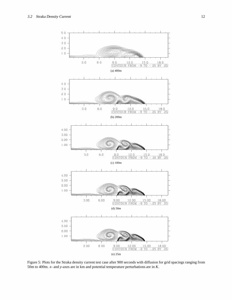
We define∆θ = −15 K, xR = 4 km, zR = 2 km, xc = 0 km, andzc = 3 km. The model domain is[−26.5,26.5]×[0,6.4] km with a grid spacing varying from 25m to 400m. The simulation is run for 900 seconds with a maximum

Courant number of 0.97 and a maximum wave speed of∣∣∣~V

∣∣∣+cs ≈ 385ms−1 . This is a good test case for examining

the oscillatory properties of a scheme because of the many strong gradients in both the wind and potential temperature.For proper grid convergence, the test case prescribes a dynamic viscosity. To accommodate this, we include simple

centered second-order accurate finite difference approximations to diffusion terms for the momentum equations andentropy equation. The horizontal momentum, vertical momentum, and entropy diffusion terms are given, respectively,by ρK (uxx+uzz), ρK (wxx+wzz), andρK (θxx+ θzz) whereK = 75m2s−1 is the coefficient of diffusion. Even thoughviscosity is present, we use free slip boundary conditions at the domain bottom (meaning the wind is not forced tozero there).

Fig. 5 shows potential temperature perturbation contours for resolutions at 400m, 200m, 100m, 50m, and 25m.Table 1 gives the maximum and minimum potential temperatureperturbation at 900 seconds of simulation. The lackof a 0 K perturbation contour is solely for the sake of plot clarity.

The plots are in line with other studies. One thing to keep in mind which makes this simulation slightly differentthan others is that we initialize the model with cell averages computed via quadrature and not cell midpoint values.Therefore, our minimum potential temperature perturbation will be slightly smaller in magnitude than other studies.We remark that a maximum potential temperature above zero does not necessarily indicate oscillations because theflow is not non-divergent.

We also ran this test inviscid to show off the stability of thescheme at Courant numbers near 1 and near 2. Fig. 6shows a plot of the inviscid density current test case run at amaximum CFL of 0.98 and 1.95 with no diffusion applied.The gradients are much stronger, and even more so than visible in the plot because we contoured at an interval of 0.5instead of 0.25 for visual purposes. This creates even more difficulty for a numerical method to remain stable, butthe WENO interpolants are sufficient for stability. For the inviscid simulation at CFLmax=0.98, the minimumθ ′

was-12.1 K and the maximumθ ′

was 0.383 K. There are noticeable differences between the two runs at near unity CFLand larger CFL which demonstrate the potential advantages of improving trajectory calculations. Still, for a turbulentflow they are very similar, and stability was maintained at the higher CFL without diffusion.

3.2 Straka Density Current 12

(a) 400m

(b) 200m

(c) 100m

(d) 50m

(e) 25m

Figure 5: Plots for the Straka density current test case after 900 seconds with diffusion for grid spacings ranging from50m to 400m.x- andy-axes are in km and potential temperature perturbations arein K.

3.3 Non-Hydrostatic Internal Gravity Waves 13

(a) CFLmax=0.98

(b) CFLmax=1.95

Figure 6: Contours of potential temperature perturbation for the Straka density current test case without numericalviscosity after 900 seconds without diffusion with a grid spacing of 50m. x- and y-axes are in km and potentialtemperature perturbations are inK.

∆z 400m 200m 100m 50m

L1 0.422339 0.156702 0.0236569 0.00172828L2 0.449548 0.187334 0.0356143 0.00300876L∞ 0.480062 0.234141 0.0703918 0.00899815

Table 2: Error norms in the potential temperature field compared to 25m results.

3.3. Non-Hydrostatic Internal Gravity Waves

Here, we test the proposed scheme in its handling of InternalGravity Waves (IGWs) on a non-hydrostatic scale.The domain is initialized with a constant Brunt-Vaisala frequency ofN = 10−2 s−1 to admit IGWs, and hydrostaticbalance is used based on this constant. A potential temperature perturbation is added to the potential temperature fieldas follows:

θ = θ0 (z)+ ∆θsin(πz/H)

1+(x−x0)2/a2

whereH = 10 km,∆θ = 10−2 K, a = 5 km, andx0 = 100 km. The simulation is run for 3,000 seconds on a domainof [0,300]× [0,10] km with a maximum Courant number of about 0.99. The initial vertical wind is set to 0 m s−1,and the initial horizontal wind is set to 20 m s−1 to advect the entire IGW train in the positivex-direction. We ran thissimulation at three vertical grid spacings ranging from 50mto 200m. The horizontal grid spacing is always ten timesgreater than the vertical in this test case.

Fig. 7 gives contour plots of the potential temperature perturbation, and Fig. 8 gives the potential temperatureperturbations along the linez= 5kmafter 3,000 seconds. These results agree well with previousstudies, and it is theonly test case which really converges to a solution as the grid is refined without requiring diffusion. Therefore, we usethis test case to get some notion of the numerical convergence of the scheme as both grid and time step are refined usingthe 25m grid spacing as the “exact” solution. If we consider the error as a function of grid spacing,E (∆x) = C(∆xn)with C being a constant with respect to∆x, then the order of convergence is given byn = ln(E (∆x)/E(∆x/ f ))/ ln f .We estimate error norms by regridding the 50m potential temperature perturbations to the coarser grid. Table 2 sumsthe error norms, and Fig. 9 shows a log-log plot with the slopeshowing the convergence. TheL1 error norms seem tobe asymptoting to near fourth-order convergence, and theL∞ norms converge more slowly which is typical.


−0.001

0.000

0.001

0.002

0 50 100 150 200 250 30002468

10

x (km)

z (k

m)

(a) ∆z=200m

−0.001

0.000

0.001

0.002

0 50 100 150 200 250 30002468

10

x (km)

z (k

m)

(b) ∆z=100m

−0.001

0.000

0.001

0.002

0 50 100 150 200 250 30002468

10

x (km)

z (k

m)

(c) ∆z=50m

Figure 7: Plots for the internal gravity waves test case after 3,000 seconds with a range of grid spacings withCFLmax=0.99. ∆x = 10∆z for all simulations. Thex- andy-axes are in km and potential temperature perturbationsare inK.


Figure 8: Plot of potential temperature perturbations along the linez= 5km for the internal gravity waves test caseafter 3,000 seconds with a range of grid spacings.∆x = 10∆z for all simulations. Thex-axis is in km and they-axis isin K.

0.01

0.1

100

Err

or

Grid spacing

L1L2

Linf3rd-order4th-order

Figure 9: Log-log plot of potential temperature errors (increasing upward) as a function of grid spacing (decreasing tothe right). We used the 25m run to represent the exact answer with lines denoting order of convergence.


−0.001

0.000

0.001

0.002

0 50 100 150 200 250 30002468

10

x (km)

z (k

m)

(a) ∆z=100m, CFLmax=1.99

−1.5e−05−1.0e−05−5.0e−060.0e+005.0e−061.0e−051.5e−05

0 50 100 150 200 250 30002468

10

x (km)

z (k

m)

(b) Differences between CFL=1.99 and CFL=0.99

Figure 10: Plots for the internal gravity waves test case after 3,000 seconds with a maximum CFL of 1.99.∆x =10∆z= 1,000 m. Thex- andy-axes are in km and potential temperature perturbations arein K.

We also ran the 100m (vertical) grid spacing run with CFLmax=1.99, and the potential temperature shaded con-tours are given in Fig. 10 along with the differences from theprevious 100m run. The maximum deviation fromthe previous run was only 1.5×10−5K which represents 0.5%. Because this is such a smooth flow with such smallchanges in characteristic velocities, we also ran the test case at a CFL of 2.99 and 3.99 with plots shown in Fig. 11 andFig. 12. For CFLmax=2.99 and CFLmax=3.99, the maximum deviations from the standard run were 1.1% and 2.0%,respectively. The maximum difference in potential temperature from CFL=0.99 as CFL increases (running with CFLup to 7) fits a quadratic function with an squared residual of 0.997 (see Table 3). Future work is necessary to find whatleads to this quadratic relationship.

With the runs of CFL > 1, there are vertically-oriented oscillations of wavelength 2CFLmax∆z in the differenceplots. We hypothesize by the wavelength scale and vertical orientation that they are due to the negative verticalgradient in the speed of sound not being captured by our assumption of constant wave speed. The fact that we obtainedbetter results for smoother flows in which characteristic trajectory gradients are small supports the hypothesis madein [36, 21] regarding accuracy, CFL, and characteristics gradients. Also, the fact that the only appreciable trajectory

CFL 1.99 2.99 3.99 4.99 5.99 6.99

Max. Abs. Diff. 1.505e-5 3.259e-5 5.295e-5 8.370e-5 1.383e-4 1.709e-4

Table 3: Maximum absolute difference of potential temperature from the CFL=0.99 run with increasing CFL.


−0.001

0.000

0.001

0.002

0 50 100 150 200 250 30002468

10

x (km)

z (k

m)

(a) ∆z=100m, CFLmax=2.99

−3e−05−2e−05−1e−050e+001e−052e−053e−05

0 50 100 150 200 250 30002468

10

x (km)

z (k

m)




−0.001

0.000

0.001

0.002

0 50 100 150 200 250 30002468

10

x (km)

z (k

m)

(a) ∆z=100m, CFLmax=3.99

−4e−05−2e−050e+002e−054e−05

0 50 100 150 200 250 30002468

10

x (km)

z (k

m)



19

gradient is in the vertical and we observed the vertical error oscillations scaling with the CFL further support thisnotion. Along with supporting the hypothesis, it supports the notion that more accurate trajectories will reduce muchof the error.

4. Conclusions and Future Work

We have presented a new FV solver for numerical simulation ofatmospheric dynamics offering competitive ef-ficiency in terms of low communication requirements and large time steps. It is fully discrete (one-step, one-stage),upwind, spatially local, stable at large CFL numbers, and itaccommodates any single-moment spatial interpolant. Wehave described the theory and implementation of the method and performed standard non-hydrostatic atmospherictest cases for validation. The method performed accuratelyand stably in each of the test cases without the need forpost-hoc diffusion to stabilize even at large Courant numbers. In the non-hydrostatic internal gravity waves test case,we estimated a numerical convergence of roughly third- to fourth-order (depending on the error norm) for that testcase.

We would like to reemphasize that on modern computing architectures (which are distributed memory machinesthat are getting larger by the year), communication is quickly becoming the dominant limitation for many schemes.There is a great need to investigate new methods which may offer promise in this regard. In comparison to finiteelement type methods such as spectral element and discontinuous Galerkin, the present method allows larger timesteps while keeping lower communication requirements thantraditional FV methods.

Results at large CFL numbers showed degraded accuracy compared to simulation at CFL near unity. Though westill had stability at CFL numbers greater than two, the accuracy degradation beyond CFL=2 was too large for twoof the test cases. Running the smoothest test case up to CFL=7revealed some characteristics of the errors associatedwith large CFL simulation. It suggests that improving trajectories may alleviate much of the error and that properlyresolving large gradients in characteristic speeds will require the most attention.

One limitation to this method in the current theory and implementation is that it is fixed to a dimensionally splitframework. We will be investigating the potential for a genuinely multi-dimensional extension for use in curvilineargeometries that do not perform as well when dimensionally split.

All simulations in this study were performed on Graphics Processing Units (GPUs). Code run on an Nvidia GTX280 GPU in double precision without exhaustive memory optimizations performed over 20x faster than OpenMP op-timized code on an Intel Core2 Duo T7500 CPU. This speed-up includes all DMA (Direct Memory Access) transfers.For the highest resolution simulations, we ran our code on 8 GPUs with MPI (Message Passing Interface) commu-nication in between different GPUs. Even with low bandwidthnetwork interconnect, we still obtained a speed-up ofover 110x, and all MPI communication times are included in that timing. The presented algorithm makes efficient useof the GPUs even without lengthy memory optimizations because most of the operations are densely clustered insidethe kernels with low communication requirements during a time step.

Acknowledgements

The first author gratefully acknowledges funding by the Department of Energy Computational Science GraduateFellowship and also partial support by the National Center for Atmospheric Research Advanced Study Program.

References

[1] N. Ahmad. The f-wave Riemann solver for meso- and micro-scale flows.AIAA Paper, 2008-465, 2008.

[2] N. Ahmad and J. Lindeman. Euler solutions using flux-based wave decomposition.International Journal forNumerical Methods in Fluids, 54:47–72, 2007.

[3] G. M. Amdahl. Validity of the single processor approach to achieving large scale computing capabilities. InProceedings of the April 18-20, 1967, spring joint computerconference, AFIPS Joint Computer Conferences,pages 483–485, 1967.

[4] D. Bale, R. J. Leveque, S. Mitran, and J. A. Rossmanith. A wave propagation method for conservation laws andbalance laws with spatially varying flux functions.SIAM Journal on Scientific Computing, 24(3):955–978, 2002.

REFERENCES 20

[5] D. S. Balsara, C. Altmann, C-D. Munz, and M. Dumbser. A sub-cell based indicator for troubled zones inRKDG schemes and a novel class of hybrid RKDG+HWENO schemes.Journal of Computational Physics,226:586–620, 2007.

[6] L. Bonaventura. A semi-implicit semi-Lagrangian scheme using the height coordinate for a nonhydrostatic andfully elastic model of atmospheric flows.Journal of Computational Physics, 227:3849–3877, 2000.

[7] G. Capdeville. A central WENO scheme for solving hyperbolic conservation laws on non-uniform meshes.Journal of Computational Physics, 227:2977–3014, 2008.

[8] Richard L. Carpenter, Kelvin K. Droegemeier, Paul R. Woodward, and Carl E. Hane. Application of the PiecewiseParabolic Method (PPM) to meteorological modeling.Monthly Weather Review, 118:586–612, 1990.

[9] M. J. P. Cullen and T. Davies. A conservative split-explicit integration scheme with fourth-order horizontaladvection.Quarterly Journal of the Royal Meteorological Society, 117:993–1002, 1991.

[10] J. M. Dennis, A. Fournier, W. F. Spotz, A. St-Cyr, M. A. Taylor, S. J. Thomas, and H. M. Tufo. High-resolutionmesh convergence properties and parallel efficiency of a spectral element atmospheric dynamical core.Interna-tional Journal of High Performance Computing Applications, 19:225–235, 2005.

[11] J. M. Dennis, R. D. Nair, H. M. Tufo, M. N. Levy, and T. Voran. Development of a scalable global discontinuousGalerkin atmospheric model.International Journal of Computational Science Engineering, page in press, 2009.

[12] D. R. Durran. The third-order adams-bashforth method:An attractive alternative to leapfrog time differencing.Monthly Weather Review, 119:702–720, 1991.

[13] K. J. Evans, W. I. Rouson, A. G. Salinger, M. A. Taylor, W.Weijer, and J. B. White. A scalable and adaptablesolution framework within components of the community climate system model. InComputational Science –ICCS 2009, volume 5545 ofLecture Notes in Computer Science, pages 332–341. Springer, 2009.

[14] A. J. Gadd. A split explicit integration scheme for numerical weather prediction.Quarterly Journal of the RoyalMeteorological Society, 104:569–582, 1978.

[15] F. X. Giraldo and M. Restelli. A study of spectral element and discontinuous Galerkin methods for the Navier–Stokes equations in nonhydrostatic mesoscale atmosphericmodeling: Equation sets and test cases.Journal ofComputational Physics, 227:3849–3877, 2008.

[16] J. L. Gustafson. Reevaluating amdahl’s law.Communications of the ACM, 31:532–533, 1988.

[17] J. B. Klemp, W. C. Skamarock, and J. Dudhia. Conservative split-explicit time integration methods for thecompressible nonhydrostatic equations.Monthly Weather Review, 135:2897–2913, 2007.

[18] D. A. Knoll and D. E. Keyes. Jacobian-free Newton–Krylov methods: a survey of approaches and applications.Journal of Computational Physics, 193:357–397, 2004.

[19] R. J. Leveque.Finite Volume Methods for Hyperbolic Problems. Cambridge University Press, Cambridge, MA,2002.

[20] M. N. Levy, R. D. Nair, and H. M. Tufo. High-order Galerkin methods for scalable global atmospheric models.Computers and Geosciences, 33:1022–1035, 2007.

[21] S. Li and F. Xiao. CIP/multi-moment finite volume methodfor Euler equations: A semi-Lagrangian characteristicformulation.Journal of Computational Physics, 222:849–871, 2007.

[22] S. Li and F. Xiao. High order multi-moment constrained finite volume method. part I: Basic formulation.Journalof Computational Physics, 228:3669–3707, 2009.

[23] D. Majewski, D. Liermann, P. Prohl, B. Ritter, M. Buchhold, T. Hanisch, G. Paul, W. Wergen, and J. Baumgard-ner. The operational global icosahedral–hexagonal gridpoint model GME: Description and high-resolution tests.Monthly Weather Review, 130:319–338, 2002.

REFERENCES 21

[24] Y. Matsumoto and K. Seki. Implementation of the CIP algorithm to magnetohydrodynamic simulations.Com-puter Physics Communications, 179:289–296, 2008.

[25] R. D. Nair, H-W. Choi, and H. M. Tufo. Computational aspects of a scalable high-order discontinuous Galerkinatmospheric dynamical core.Computers and Fluids, 38:309–319, 2009.

[26] R. D. Nair, S. J. Thomas, and R. D. Loft. A discontinuous Galerkin transport scheme on the cubed sphere.Monthly Weather Review, 133(4):814–828, April 2005.

[27] M. R. Norman and R. D. Nair. Inherently conservative non-polynomial based remapping schemes: Applicationto semi-Lagrangian transport.Monthly Weather Review, 136:5044–5061, 2008.

[28] M. R. Norman, F. H. M. Semazzi, and R. D. Nair. Conservative cascade interpolation on the sphere: An inter-comparison of various non-oscillatory reconstructions.Quarterly Journal of the Royal Meteorological Society,135:795–805, 2009.

[29] F. H. M. Semazzi, J. H. Quian, and J. S. Scroggs. A global nonhydrostatic semi-Lagrangian atmospheric modelwithout orography.Monthly Weather Review, 123:2534, 1995.

[30] C. W. Shu. High order ENO and WENO schemes for computational fluid dynamics. In T. J. Barth and H. De-coninck, editors,High-Order Methods for Computational Physics, volume 9 ofLecture Notes in ComputationalScience and Engineering, pages 439–582. Springer, 1999.

[31] C. W. Shu and S. Osher. Efficient implementation of essentially non-oscillatory shock-capturing schemes.Jour-nal of Computational Physics, 77:439–471, 1988.

[32] W. C. Skamarock and J. B. Klemp. A time-split nonhydrostatic atmospheric model for weather research andforecasting applications.Journal of Computational Physics, 227:3465–3485, 2008.

[33] P. K. Smolarkiewicz, L. G. Margolin, and A. A. Wyszogrodzki. A class of nonhydrostatic global models.Journalof the Atmospheric Sciences, 58:349–364, 2001.

[34] A. Staniforth and J. Cote. Semi-Lagrangian integration schemes for atmospheric models: A review.MonthlyWeather Review, 119(9):2206–2223, September 1991.

[35] J. M. Straka, R. B. Wilhelmson, L. J. Wicker, J. R. Anderson, and K. K. Droegemeier. Numerical solutionsof a non-linear density current: A benchmark solution and comparisons.International Journal for NumericalMethods in Fluids, 17:1–22, 1993.

[36] K. Toda, Y. Ogata, and T. Yabe. Multi-dimensional conservative semi-Lagrangian method of characteristics CIPfor the shallow water equations.Journal of Computational Physics, 228:4917–4944, 2009.

[37] H. Wang, J. J. Tribbia, F. Baer, A. Fournier, and M. A. Taylor. A spectral element version of CAM2.MonthlyWeather Review, 135:3825–3840, 2007.

[38] T. Yabe and Y. Ogata. Conservative semi-Lagrangian CIPtechnique for the shallow water equations.Computa-tional Mechanics, 2009.

a low communication and large time step explicit finite

Documents