time-efficient variants of twin support vector … · iii certi cate this is to certify that the...
TRANSCRIPT

TIME-EFFICIENT VARIANTS OF TWIN SUPPORT
VECTOR MACHINE WITH APPLICATIONS IN
IMAGE PROCESSING
by
POOJA SAIGAL
Department of Computer Science
Submitted
in fulfillment of the requirements of the degree of
Doctor of Philosophy
to the
South Asian University,
New Delhi, India
August, 2017

c© South Asian University (SAU), Delhi, 2017
All Rights Reserved.

Dedicated to Amit, Akaisha
and my Family


i
Declaration
I hereby declare that the thesis entitled Time-efficient Variants of Twin
Support Vector Machine with Applications in Image Processing being
submitted to the South Asian University, New Delhi for the award of the degree of
Doctor of Philosophy contains the original work carried out by me under the super-
vision of Dr. Reshma Rastogi. The research work reported in this thesis is original
and has not been submitted either in part or full to any university or institution for
the award of any degree or diploma.
Pooja Saigal
Enrollment No.: SAU/CS(P)/2013/004


iii
Certificate
This is to certify that the thesis entitled “Time-efficient Variants of Twin
Support Vector Machine with Applications in Image Processing submit-
ted by Pooja Saigal to the South Asian University, New Delhi for the award of the
degree of Doctor of Philosophy, is a record of the bonafide research work carried out
by her under my supervision and guidance. The thesis has reached the standards
fulfilling the requirements of the regulations relating to the degree.
The results contained in this thesis have not been submitted in part or full to any
other university or institute for the award of any degree or diploma.
Dr. Reshma Rastogi
(Supervisor)
Department of Computer Science,
South Asian University,
New Delhi, India


v
Acknowledgments
The tenure of my Ph.D. at South Asian University has been an enriching and
fruitful experience. I am indebted to many people who made this work possible and
it is my pleasure to express my gratitude towards them.
I owe my deepest gratitude to my supervisor Dr. Reshma Rastogi. Working
with her has been a real pleasure to me, with tremendous learning and growth. She
has been a steady support throughout the duration of my Ph.D. and has oriented
me with promptness. She has always been patient and encouraging in times of new
ideas and difficulties. The discussions with her have led to key insights. Her ability
to identify and approach compelling research problems with high scientific standards
and hard work, motivated me to give my best to this research work. I also admire
her for making me feel like a friend. I could not have imagined having a better
supervisor and mentor for my research work.
I am extremely thankful to Dr. Suresh Chandra, for his valuable suggestions
and encouragement that improved the quality of my research work. It is very dif-
ficult to find a person like Dr. Chandra who is so humble and has an astounding
understanding of mathematics. I have been very privileged to get to know him and
to work with him.
I am extremely grateful to South Asian University for providing the financial
support, in the form of scholarship, to carry out this work. I also thank SAU for
providing a conducive environment and a well equipped Machine Learning and Com-
putational Intelligence Laboratory. I am grateful to Dr. Kavita Sharma (President,
SAU). I would like to express my gratitude towards Dean, Faculty of Mathematics
and Computer Science, Dr. R.K.Mohanty and Chairperson, Department of Com-
puter Science Dr. Muhammad Abulaish, for their support and encouragement. I am
also thankful to Dr. Pranab K. Muhuri, Dr. Amit Banerjee and Dr.Danish Lohani.
I am grateful to all the members of DRC. I am thankful to my RPC members Dr.
Deepa Sinha (Department of Mathematics) and Dr. Muhammad Abulaish, for their
valuable suggestions and encouragement. I also owe my gratitude towards Dr. Ekta
Walia for her help during my initial days of Ph.D. Coursework.
The last four years have been a period of immense learning with extensive work

vi
and I would like to thank all my colleagues for proving an excellent research en-
vironment. I appreciate their support and cooperation during my stay at SAU. I
am thankful to Aman Pal, Sweta Sharma, Pritam Anand and Yashi for being great
friends and supporting me at the time of need. The discussions with them stimu-
lated new ideas and gave different perspectives for handling a problem. I would like
to thank all my colleagues from the Department of Computer Science and Mathe-
matics.
Finally, I would like to thank most important people in my life. This thesis
would not have been possible without their constant support and encouragement.
My husband Amit Saigal is my strength. He supported me unconditionally in every
sphere of life and has motivated me throughout my research work at SAU. I have
learnt the qualities of perseverance and dedication from him. There were multiple
times when I felt dejected and he helped me out. I will never be able to thank
him enough for his steady support at difficult times. These four years have been
a learning experience for my loving daughter Akaisha, who has learnt to be inde-
pendent as I was not always there to help her. I am grateful to my parents-in-law
who supported me with great patience and took upon my responsibilities at home,
in my absence. I am grateful to God that I am born in a family who is so caring
and supportive. I could not thank my mother Mrs. Neelam Khanna enough, for
supporting me emotionally and listening to all my feelings. I am blessed to have
Nidhi and Vaibhav as my siblings, whose love and support helped me to get out
of hard times. My idol is my father Mr. Shiv Kumar Khanna, who is showering
his blessings on me from heaven. He always inspired me and had firm belief in my
capabilities.
Pooja Saigal

vii
Preface
Human beings can display behavior that can be called as intelligent, by learning
from the experiences. Learning gives us flexibility to adapt and adjust to new envi-
ronment. The aim of learning is to generalize which essentially means to establish
similarity between situations, so that the rules which are applicable in one situa-
tion can be applied or extended to other situations. Machine learning is a rapidly
progressing stream of artificial intelligence that enables a machine to learn from
the empirical data and builds models to make reliable future predictions. Depend-
ing on the availability of output values (labels), machine learning can be broadly
categorized into two paradigms: supervised and unsupervised learning.
One of the most distinguished works in supervised learning is classification using
Support Vector Machines (SVMs). Another major breakthrough is the develop-
ment of Twin Support Vector Machine (TWSVM) which has better generalization
ability than SVM and is almost four times faster than conventional SVMs. This re-
search work is an attempt to explore the existing SVM and TWSVM based learning
algorithms and to develop new ones which could deliver better results than well-
established methodologies. Our focus is on development of time-efficient supervised
and unsupervised TWSVM-based learning algorithms, with good generalization abil-
ity, and to apply them for image processing tasks.
This thesis presents novel nonparallel hyperplane classification algorithms along
with their extension to multi-category classification and clustering approaches. Im-
provements on ν-Twin Support Vector Machine (Iν-TWSVM) is a classification
algorithm which solves a smaller-sized quadratic programming problem (QPP) and
an unconstrained minimization problem (UMP), instead of solving a pair of QPPs
as done for TWSVM, to generate two nonparallel proximal hyperplanes. The faster
version of Iν-TWSVM, termed as Iν-TWSVM (Fast), modifies the first problem of
Iν-TWSVM as minimization of a unimodal function for which line search methods
can be used; this further avoids solving the QPP in the first problem. Both these
classifiers have good generalization ability. Two more classifiers i.e. Angle-based
Twin Parametric-Margin Support Vector Machine (ATP-SVM) and Angle-based
Twin Support Vector Machine (ATWSVM), have been developed which try to max-

viii
imize the angle between the normal vectors to the two nonparallel hyperplanes so
as to generate larger separation between the two classes. ATP-SVM solves only one
modified QPP with fewer number of representative patterns. It avoids the explicit
computation of inverse of matrices in the dual problem and has efficient learning
time. ATWSVM finds the two hyperplanes by solving a QPP and a UMP.
This work presents a multi-category classification algorithm termed as Reduced
tree for Ternary Support Vector Machine (RT-TerSVM), which organizes the clas-
sifiers in the form of a ternary tree. This algorithm uses a novel classifier Ternary
Support Vector Machine (TerSVM) to generate three nonparallel hyperplanes. An-
other novel multi-category classification algorithm termed as Ternary Decision Struc-
ture (TDS) has been developed that can extend binary classifiers to multi-category
framework. TDS is more time efficient than the classical One-Against-All (OAA)
approach. For a K-class problem, a balanced TDS requires dlog3Ke comparisons for
evaluating a test pattern. TDS associates ternary output labels +1, 0 or −1 with
the training patterns. Another multi-category approach Binary Tree (BT) of classi-
fiers is developed on the lines of TDS and it generates binary output at each level of
the tree. Our work compares the behavior of nonparallel hyperplanes classifiers viz.
Generalized Eigenvalue Proximal SVM (GEPSVM) and its variants, using different
multi-category approaches.
This work includes development of an unsupervised clustering algorithm termed
as Tree-based Localized Fuzzy Twin Support Vector Clustering (Tree-TWSVC),
which recursively builds a cluster model as a Binary Tree. Here, each node com-
prises of a novel TWSVM-based classifier termed as Localized Fuzzy TWSVM (LF-
TWSVM). Since there is uncertainty in associating cluster labels with patterns, so we
used fuzzy cluster membership. Tree-TWSVC has efficient learning time, achieved
due to tree structure and its formulation leads to solving a series of system of linear
equations. All the above mentioned classification and clustering algorithms have
been applied to perform image processing tasks like content based image retrieval,
image segmentation and handwritten digit recognition.

ix
List of Publications
Papers in Journals:
1. Rastogi, R., Saigal, P. and Chandra, S., 2018: Angle-based Twin Parametric-
margin Support Vector Machine for Pattern Classification. Knowledge-
Based Systems, 139, pp. 64-77.
2. Rastogi, R., Saigal, P. and Chandra, S., 2017. Angle-based Twin Support
Vector Machine. Annals of Operations Research, DOI: 10.1007/s10479-
017-2604-2.
3. Rastogi, R. and Saigal, P., 2017. Tree-based Localized Fuzzy Twin Support
Vector Clustering with Square Loss Function. Applied Intelligence, 47 (1),
pp. 96-113.
4. Khemchandani, R., Saigal, P. and Chandra, S., 2016. Improvements on ν-
Twin Support Vector Machine. Neural Networks, 79, pp. 97-107.
5. Khemchandani, R. and Saigal, P., 2015. Color Image Classification and Re-
trieval Through Ternary Decision Structure Based Multi-category TWSVM.
Neurocomputing, 165, pp. 444-455.
Conference proceedings:
5. Saigal, P. and Khemchandani, R., 2015, December. Nonparallel Hyperplane
Classifiers for Multi-category Classification. 2015 IEEE Workshop on Compu-
tational Intelligence: Theories, Applications and Future Directions (WCI), pp.
1-6.
Communicated Papers:
1. Saigal, P., Rastogi, R. and Chandra, S.: Ternary Support Vector Machine
with Extension for Multi-category Classification.

x

Table of Contents
Declaration . . . . . . . . . . . . . . . . . . . . . . . . . . . . . . . . . . . . . . . . . . i
Certificate . . . . . . . . . . . . . . . . . . . . . . . . . . . . . . . . . . . . . . . . . . . iii
Acknowledgments . . . . . . . . . . . . . . . . . . . . . . . . . . . . . . . . . . . . . . v
Preface . . . . . . . . . . . . . . . . . . . . . . . . . . . . . . . . . . . . . . . . . . . . vii
List of Publications . . . . . . . . . . . . . . . . . . . . . . . . . . . . . . . . . . . . . ix
List of Figures . . . . . . . . . . . . . . . . . . . . . . . . . . . . . . . . . . . . . . . . xvi
List of Tables . . . . . . . . . . . . . . . . . . . . . . . . . . . . . . . . . . . . . . . . . xviii
List of Symbols . . . . . . . . . . . . . . . . . . . . . . . . . . . . . . . . . . . . . . . . xviii
1. Introduction . . . . . . . . . . . . . . . . . . . . . . . . . . . . . . . . . . . . . . . 1
1.1. Classification Techniques . . . . . . . . . . . . . . . . . . . . . . . . . . . . . . 3
1.1.1. Twin Support Vector Machine . . . . . . . . . . . . . . . . . . . . . . . 3
1.1.2. Least Square Twin Support Vector Machine . . . . . . . . . . . . . . . 6
1.1.3. Twin Bounded Support Vector Machine . . . . . . . . . . . . . . . . . 7
1.1.4. Twin Parametric-Margin Support Vector Machine . . . . . . . . . . . . 8
1.1.5. ν-Twin Support Vector Machine . . . . . . . . . . . . . . . . . . . . . . 9
1.1.6. Nonparallel Support Vector Machine with One Optimization Problem . 10
1.2. Clustering Techniques . . . . . . . . . . . . . . . . . . . . . . . . . . . . . . . 10
1.2.1. K-Means Clustering . . . . . . . . . . . . . . . . . . . . . . . . . . . . . 11
1.2.2. Maximum-Margin Clustering . . . . . . . . . . . . . . . . . . . . . . . . 11
1.2.3. Twin Support Vector Machine for Clustering . . . . . . . . . . . . . . 12
1.3. Multi-Category Extension of Binary Classifiers . . . . . . . . . . . . . . . . . 14
1.3.1. One-Against-One Twin Support Vector Machine . . . . . . . . . . . . . 15
1.3.2. Twin-KSVC . . . . . . . . . . . . . . . . . . . . . . . . . . . . . . . . . 16
1.4. Brief Introduction to Image Processing . . . . . . . . . . . . . . . . . . . . . . 16
1.4.1. Content-based Image Retrieval . . . . . . . . . . . . . . . . . . . . . . . 17
1.4.2. Image Classification . . . . . . . . . . . . . . . . . . . . . . . . . . . . . 17
1.4.3. Image Segmentation through Pixel Classification . . . . . . . . . . . . . 17
1.5. Contribution of the Thesis . . . . . . . . . . . . . . . . . . . . . . . . . . . . . 17

xii
2. Improvements on ν-Twin Support Vector Machine . . . . . . . . . . . . . . . . . . 23
2.1. Introduction . . . . . . . . . . . . . . . . . . . . . . . . . . . . . . . . . . . . . 23
2.2. Improvements on ν-Twin Support Vector Machine . . . . . . . . . . . . . . . 24
2.2.1. Iν-TWSVM (Linear classifier) . . . . . . . . . . . . . . . . . . . . . . . 25
2.2.2. Iν-TWSVM (Kernel classifier) . . . . . . . . . . . . . . . . . . . . . . . 29
2.3. Improvements on ν-Twin Support Vector Machine (Fast) . . . . . . . . . . . 31
2.4. Multi-category Extensions of Iν-TWSVM . . . . . . . . . . . . . . . . . . . . 32
2.4.1. One-Against-All Iν-TWSVM . . . . . . . . . . . . . . . . . . . . . . . . 32
2.4.2. Binary Tree of Iν-TWSVM . . . . . . . . . . . . . . . . . . . . . . . . . 33
2.5. Discussion . . . . . . . . . . . . . . . . . . . . . . . . . . . . . . . . . . . . . . 33
2.6. Experimental Results . . . . . . . . . . . . . . . . . . . . . . . . . . . . . . . . 34
2.6.1. Synthetic Datasets . . . . . . . . . . . . . . . . . . . . . . . . . . . . . 35
2.6.2. Binary Classification Results: UCI and Exp-NDC datasets . . . . . . . 36
2.6.3. Statistical Tests . . . . . . . . . . . . . . . . . . . . . . . . . . . . . . . 40
2.6.4. Scatter Plots . . . . . . . . . . . . . . . . . . . . . . . . . . . . . . . . . 42
2.6.5. Multi-category Classification Results: UCI Datasets . . . . . . . . . . . 44
2.7. Application: Image Segmentation . . . . . . . . . . . . . . . . . . . . . . . . . 44
2.8. Conclusions . . . . . . . . . . . . . . . . . . . . . . . . . . . . . . . . . . . . . 46
3. Angle-based Nonparallel Hyperplanes Classifiers . . . . . . . . . . . . . . . . . . . 47
3.1. Introduction . . . . . . . . . . . . . . . . . . . . . . . . . . . . . . . . . . . . . 47
3.2. Angle-based Twin Parametric-Margin Support Vector Machine . . . . . . . . 49
3.2.1. Selection of Representative Points . . . . . . . . . . . . . . . . . . . . . 49
3.2.2. ATP-SVM (Linear version) . . . . . . . . . . . . . . . . . . . . . . . . . 50
3.2.3. ATP-SVM (Kernel version) . . . . . . . . . . . . . . . . . . . . . . . . . 53
3.3. Angle-based Twin Support Vector Machine . . . . . . . . . . . . . . . . . . . 55
3.3.1. ATWSVM (Linear version) . . . . . . . . . . . . . . . . . . . . . . . . . 56
3.3.2. ATWSVM (Kernel version) . . . . . . . . . . . . . . . . . . . . . . . . . 59
3.4. Other Versions of ATWSVM . . . . . . . . . . . . . . . . . . . . . . . . . . . 60
3.5. Multi-category Extension of ATP-SVM and ATWSVM . . . . . . . . . . . . . 63
3.6. Discussion . . . . . . . . . . . . . . . . . . . . . . . . . . . . . . . . . . . . . . 63
3.7. Experimental Results . . . . . . . . . . . . . . . . . . . . . . . . . . . . . . . . 67
3.7.1. Synthetic Datasets . . . . . . . . . . . . . . . . . . . . . . . . . . . . . 67
3.7.2. Binary Classification Results: UCI and NDC Datasets . . . . . . . . . 70
3.7.3. Statistical Tests . . . . . . . . . . . . . . . . . . . . . . . . . . . . . . . 77
3.7.4. Multi-category Classification Results: UCI Datasets . . . . . . . . . . . 78
3.8. Application: Segmentation through Pixel Classification of Color Images . . . 80

xiii
3.9. Conclusions . . . . . . . . . . . . . . . . . . . . . . . . . . . . . . . . . . . . . 82
4. Ternary Support Vector Machine with Extension for Multi-category Classification 87
4.1. Introduction . . . . . . . . . . . . . . . . . . . . . . . . . . . . . . . . . . . . . 87
4.2. Ternary Support Vector Machine . . . . . . . . . . . . . . . . . . . . . . . . . 89
4.2.1. TerSVM (Linear version) . . . . . . . . . . . . . . . . . . . . . . . . . . 90
4.2.2. TerSVM (Kernel version) . . . . . . . . . . . . . . . . . . . . . . . . . . 94
4.2.3. TerSVM as Binary Classifier . . . . . . . . . . . . . . . . . . . . . . . . 96
4.3. Multi-category Classification Algorithm: Reduced Tree for TerSVM . . . . . . 96
4.4. Discussion . . . . . . . . . . . . . . . . . . . . . . . . . . . . . . . . . . . . . . 100
4.5. Experimental Results . . . . . . . . . . . . . . . . . . . . . . . . . . . . . . . . 104
4.5.1. Synthetic Dataset . . . . . . . . . . . . . . . . . . . . . . . . . . . . . . 105
4.5.2. Multi-category Classification Results: UCI Datasets . . . . . . . . . . . 105
4.6. Applications . . . . . . . . . . . . . . . . . . . . . . . . . . . . . . . . . . . . . 110
4.6.1. Hand-written Digits Recognition: USPS Dataset . . . . . . . . . . . . . 110
4.6.2. Color Image Classification . . . . . . . . . . . . . . . . . . . . . . . . . 111
4.7. Conclusions . . . . . . . . . . . . . . . . . . . . . . . . . . . . . . . . . . . . . 112
5. Multi-category Classification Approaches for Nonparallel Hyperplanes Classifiers . 115
5.1. Introduction . . . . . . . . . . . . . . . . . . . . . . . . . . . . . . . . . . . . . 115
5.2. Ternary Decision Structure . . . . . . . . . . . . . . . . . . . . . . . . . . . . 117
5.2.1. Binary Tree Multi-category Approach . . . . . . . . . . . . . . . . . . . 119
5.2.2. Content-based Image Classification using TDS-TWSVM . . . . . . . . 120
5.2.3. Content-based Image Retrieval using TDS-TWSVM . . . . . . . . . . . 121
5.2.4. Comparison of TDS-TWSVM with Other Multi-Category Approaches . 122
5.3. Eigenvalue Problem Based Classifiers . . . . . . . . . . . . . . . . . . . . . . . 122
5.3.1. Generalized Eigenvalue Proximal Support Vector Machine . . . . . . . 123
5.3.2. Regularized GEPSVM . . . . . . . . . . . . . . . . . . . . . . . . . . . 124
5.3.3. Improved GEPSVM . . . . . . . . . . . . . . . . . . . . . . . . . . . . . 125
5.4. Extension of NHCAs for Multi-category Classification . . . . . . . . . . . . . 126
5.5. Experimental Results . . . . . . . . . . . . . . . . . . . . . . . . . . . . . . . . 127
5.5.1. Multi-category Classification Results: UCI Datasets . . . . . . . . . . . 127
5.6. Applications . . . . . . . . . . . . . . . . . . . . . . . . . . . . . . . . . . . . . 129
5.6.1. Color Image Classification . . . . . . . . . . . . . . . . . . . . . . . . . 130
5.6.2. Content-based Image Retrieval . . . . . . . . . . . . . . . . . . . . . . . 130
5.7. Conclusions . . . . . . . . . . . . . . . . . . . . . . . . . . . . . . . . . . . . . 134

xiv
6. Tree-Based Localized Fuzzy Twin Support Vector Clustering with Square Loss
Function . . . . . . . . . . . . . . . . . . . . . . . . . . . . . . . . . . . . . . . . . . 137
6.1. Introduction . . . . . . . . . . . . . . . . . . . . . . . . . . . . . . . . . . . . . 137
6.2. Tree-based Localized Fuzzy Twin Support Vector Clustering . . . . . . . . . . 139
6.2.1. Localized Fuzzy TWSVM Classifier (Linear version) . . . . . . . . . . . 141
6.2.2. LF-TWSVM (Kernel version) . . . . . . . . . . . . . . . . . . . . . . . 144
6.2.3. Clustering Algorithms: BTree-TWSVC and OAA-Tree-TWSVC . . . . 145
6.3. Discussion . . . . . . . . . . . . . . . . . . . . . . . . . . . . . . . . . . . . . . 150
6.4. Experimental Results . . . . . . . . . . . . . . . . . . . . . . . . . . . . . . . . 155
6.4.1. Clustering Results: UCI Datasets . . . . . . . . . . . . . . . . . . . . . 156
6.4.2. Clustering Results: Large Sized Datasets . . . . . . . . . . . . . . . . . 159
6.5. Application: Image Segmentation . . . . . . . . . . . . . . . . . . . . . . . . . 160
6.6. Conclusions . . . . . . . . . . . . . . . . . . . . . . . . . . . . . . . . . . . . . 161
7. Concluding Remarks . . . . . . . . . . . . . . . . . . . . . . . . . . . . . . . . . . . 165
7.1. Advantages of our Work . . . . . . . . . . . . . . . . . . . . . . . . . . . . . . 165
7.2. Utility and Comparative Analysis of Algorithms . . . . . . . . . . . . . . . . . 167
7.3. Pitfalls to be Avoided . . . . . . . . . . . . . . . . . . . . . . . . . . . . . . . 168
7.4. The Road-map Ahead . . . . . . . . . . . . . . . . . . . . . . . . . . . . . . . 170
References . . . . . . . . . . . . . . . . . . . . . . . . . . . . . . . . . . . . . . . . . . . 171
Appendices . . . . . . . . . . . . . . . . . . . . . . . . . . . . . . . . . . . . . . . . . . 183
A. Evaluation Measures . . . . . . . . . . . . . . . . . . . . . . . . . . . . . . . . . . . 185
B. Loss Function of TWSVM . . . . . . . . . . . . . . . . . . . . . . . . . . . . . . . . 189
C. UCI Datasets . . . . . . . . . . . . . . . . . . . . . . . . . . . . . . . . . . . . . . . 191
D. Synthetic Datasets . . . . . . . . . . . . . . . . . . . . . . . . . . . . . . . . . . . . 195
E. Image Features and Datasets . . . . . . . . . . . . . . . . . . . . . . . . . . . . . . 199
E.1. Image Descriptors . . . . . . . . . . . . . . . . . . . . . . . . . . . . . . . . . 199

List of Figures
2. Improvements on ν-Twin Support Vector Machine . . . . . . . . . . . . . . . . . .
2.1. Two moons dataset: Classification result with Iν-TWSVM . . . . . . . . . . 35
2.2. The hyperplanes obtained for cross-planes dataset . . . . . . . . . . . . . . . 36
2.3. Two-dimensional projections of 21 test data points of Thyroid dataset . . . . 43
2.4. Two-dimensional projections of 70 test data points of WPBC dataset . . . . 43
3. Angle-based Nonparallel Hyperplanes Classifiers . . . . . . . . . . . . . . . . . . .
3.1. Geometrical illustration of angle between normal vectors to ATP-SVM hy-
perplanes . . . . . . . . . . . . . . . . . . . . . . . . . . . . . . . . . . . . . . 50
3.2. Geometrical illustration of angle between normal vectors to ATWSVM hy-
perplanes . . . . . . . . . . . . . . . . . . . . . . . . . . . . . . . . . . . . . . 58
3.3. Classifiers obtained for synthetic dataset (Syn1). a. ATWSVM b. TBSVM . 61
3.4. Three-class classification with (a.) OAA-NHC (b.) BT-NHC . . . . . . . . . 64
3.5. Geometric interpretation of ATP-SVM, NSVMOOP and TPMSVM . . . . . 65
3.6. Influence of parameters on the performance of ATWSVM classifier. The
parameters c1 and c5 are assigned same value, c3=0.1 and c2 + c4 = 1 . . . . 68
3.7. Hyperplanes obtained by ATP-SVM and NSVMOOP for cross-planes dataset 69
3.8. Complex XOR dataset and the hyperplanes obtained by classifiers . . . . . . 69
3.9. Results on Ripley’s dataset with linear classifiers a. ATP-SVM b. NSV-
MOOP c. TPMSVM . . . . . . . . . . . . . . . . . . . . . . . . . . . . . . . . 70
4. Ternary Support Vector Machine with Extension for Multi-category Classification
4.1. Geometrical illustration of angle between normal vectors to the hyperplanes . 93
4.2. RT-TerSVM for dataset with 5 classes . . . . . . . . . . . . . . . . . . . . . . 97
4.3. Synthetic dataset with 300 data points. Hyperplanes obtained by a. TerSVM;
b. Twin-KSVC . . . . . . . . . . . . . . . . . . . . . . . . . . . . . . . . . . . 103
4.4. Linear TerSVM classifier with three classes . . . . . . . . . . . . . . . . . . . 105
4.5. Learning time of classifiers for UCI datasets (linear) . . . . . . . . . . . . . . 108
4.6. Learning time of classifiers for large-sized UCI datasets (linear) . . . . . . . . 108

xvi
4.7. Learning time of classifiers for UCI datasets (non-linear) . . . . . . . . . . . . 109
4.8. Learning time of classifiers for large-sized UCI datasets (non-linear) . . . . . 110
5. Multi-category Classification Approaches for Nonparallel Hyperplanes Classifiers .
5.1. Ternary Decision Structure of classifiers with 10 classes . . . . . . . . . . . . 118
5.2. Illustration of TDS-TWSVM . . . . . . . . . . . . . . . . . . . . . . . . . . . 119
5.3. Three-class problem classified by OAA and TDS . . . . . . . . . . . . . . . . 127
5.4. Image Retrieval Result for a Sample Query Image from Wang’s Dataset (a.)
Query Image (b.) 20 Images retrieved by TDS-TWSVM . . . . . . . . . . . . 132
5.5. Time Complexity Comparison of TDS-TWSVM and OAA-TWSVM . . . . . 134
6. Tree-Based Localized Fuzzy Twin Support Vector Clustering with Square Loss
Function . . . . . . . . . . . . . . . . . . . . . . . . . . . . . . . . . . . . . . . . . .
6.1. Illustration of tree of classifiers. . . . . . . . . . . . . . . . . . . . . . . . . . . 140
6.2. Learning time (Linear) . . . . . . . . . . . . . . . . . . . . . . . . . . . . . . . 160
6.3. Learning time (Non-linear) . . . . . . . . . . . . . . . . . . . . . . . . . . . . 160
6.4. Segmentation results on BSD images (a.) Original image (b.) MSS-KSC (c.)
TWSVC (d.) BTree-TWSVC . . . . . . . . . . . . . . . . . . . . . . . . . . . 162
B. Loss Function of TWSVM . . . . . . . . . . . . . . . . . . . . . . . . . . . . . . .
B.1. Flipping of labels. a. Hinge loss function; b. Square loss function . . . . . . . 190
D. Synthetic Datasets . . . . . . . . . . . . . . . . . . . . . . . . . . . . . . . . . . . .
D.1. Synthetic Datasets . . . . . . . . . . . . . . . . . . . . . . . . . . . . . . . . . 195
D.2. Two moons dataset . . . . . . . . . . . . . . . . . . . . . . . . . . . . . . . . . 197
E. Image Features and Datasets . . . . . . . . . . . . . . . . . . . . . . . . . . . . . .
E.1. Sample Wang’s Color Images . . . . . . . . . . . . . . . . . . . . . . . . . . . 204
E.2. Sample COREL 5K Images . . . . . . . . . . . . . . . . . . . . . . . . . . . . 204
E.3. Sample MIT VisTex Sub-images . . . . . . . . . . . . . . . . . . . . . . . . . 205
E.4. Sample OT-scene Images . . . . . . . . . . . . . . . . . . . . . . . . . . . . . 205
E.5. Sample USPS digits (0-9) . . . . . . . . . . . . . . . . . . . . . . . . . . . . . 206

List of Tables
2. Improvements on ν-Twin Support Vector Machine . . . . . . . . . . . . . . . . . .
2.1. Classification accuracy for synthetic datasets . . . . . . . . . . . . . . . . . . 36
2.2. Classification results with linear classifier on UCI datasets . . . . . . . . . . . 38
2.3. Classification results with linear classifier on Exp-NDC datasets . . . . . . . . 39
2.4. Classification results with non-linear classifier on UCI datasets . . . . . . . . 40
2.5. Classification result with non-linear classifier on Exp-NDC datasets . . . . . . 41
2.6. Friedman test and p-values with linear classifiers for UCI datasets . . . . . . 41
2.7. Friedman test and p-values with non-linear classifiers for UCI datasets . . . . 42
2.8. Classification results with linear multi-category classifiers for UCI datasets . . 44
2.9. Pixel Classification of color images from BSD image dataset. . . . . . . . . . 45
3. Angle-based Nonparallel Hyperplanes Classifiers . . . . . . . . . . . . . . . . . . .
3.1. Classification results with linear classifiers on binary UCI datasets . . . . . . 72
3.2. Variation in classification accuracy based on selection of classes . . . . . . . . 73
3.3. Classification results with non-linear classifier on binary UCI datasets . . . . 74
3.4. Classification results with linear classifiers on NDC datasets . . . . . . . . . . 76
3.5. Classification result with non-linear classifiers on NDC datasets . . . . . . . . 77
3.6. Friedman test ranks with linear classifiers for UCI datasets . . . . . . . . . . 78
3.7. Classification results with non-linear classifier on multi-category UCI datasets 79
3.8. Friedman test and p-values with multi-category classifiers for UCI datasets . 80
3.9. Segmentation results for BSD color images . . . . . . . . . . . . . . . . . . . . 81
3.10. Segmentation results (binary) on color images from BSD image dataset . . . 83
3.11. Segmentation results (binary) on color images from BSD image dataset . . . 84
3.12. Segmentation result for BSD color images . . . . . . . . . . . . . . . . . . . . 85
3.13. Segmentation results (multi-region) with normalized cut, K-Means and ATP-
SVM on color images of BSD dataset . . . . . . . . . . . . . . . . . . . . . . 86
4. Ternary Support Vector Machine with Extension for Multi-category Classification
4.1. Classification results with linear classifier on multi-category UCI datasets . . 106

xviii
4.2. Classification results with linear classifier on large-sized multi-category UCI
datasets . . . . . . . . . . . . . . . . . . . . . . . . . . . . . . . . . . . . . . . 106
4.3. Classification results with non-linear classifier on multi-category UCI datasets 107
4.4. Classification results with non-linear classifier on large-sized multi-category
UCI datasets . . . . . . . . . . . . . . . . . . . . . . . . . . . . . . . . . . . . 107
4.5. Classification accuracy with linear classifier on three-class datasets created
from USPS . . . . . . . . . . . . . . . . . . . . . . . . . . . . . . . . . . . . . 111
4.6. USPS Error Rate with different approaches . . . . . . . . . . . . . . . . . . . 111
4.7. Classification accuracy for image datasets . . . . . . . . . . . . . . . . . . . . 112
5. Multi-category Classification Approaches for Nonparallel Hyperplanes Classifiers .
5.1. Comparison of NHCAs with linear classifiers . . . . . . . . . . . . . . . . . . 128
5.2. Comparison of NHCAs with nonlinear classifiers . . . . . . . . . . . . . . . . 129
5.3. Classification accuracy on different image datasets . . . . . . . . . . . . . . . 130
5.4. Average Retrieval Rate (%) for Wang’s Color Dataset . . . . . . . . . . . . . 131
5.5. Average Retrieval Rate (%) for COREL 5K Dataset . . . . . . . . . . . . . . 131
5.6. Average Retrieval Rate (%) for MIT VisTex Dataset . . . . . . . . . . . . . . 133
5.7. Average Retrieval Rate(ARR) (%) for OT-Scene Dataset . . . . . . . . . . . 133
5.8. Average Time (sec) required to build the classifier . . . . . . . . . . . . . . . 134
6. Tree-Based Localized Fuzzy Twin Support Vector Clustering with Square Loss
Function . . . . . . . . . . . . . . . . . . . . . . . . . . . . . . . . . . . . . . . . . .
6.1. Clustering with TWSVC and Tree-TWSVC for four clusters . . . . . . . . . . 151
6.2. Clustering accuracy for UCI datasets (Linear version) . . . . . . . . . . . . . 157
6.3. OoS Clustering accuracy for UCI datasets (Linear version) . . . . . . . . . . . 157
6.4. Clustering accuracy for UCI datasets (Non-linear version) . . . . . . . . . . . 158
6.5. OoS Clustering accuracy for UCI datasets (Non-linear version) . . . . . . . . 159
6.6. Segmentation result for BSD color images . . . . . . . . . . . . . . . . . . . . 163

List of Symbols
α, β, γ Lagrange multiplier vectors
ηi Projection vector for ith class patterns
‖.‖2 L2-norm
Rn n-dimensional real space
ν-SVM ν-Support Vector Machine
ν-TWSVM ν-Twin Support Vector Machine
νi User defined weight associated with ρi
φ Mapping induced by the kernel function
ρi Minimum separating distance between the patterns of ith class and hyper-
plane of other class
|.| Absolute distance
ξi Slack variable or error vector for ith class
ξj+1i Slack variable for ith class in (j + 1)th iteration
A Data matrix for positive class
Ai Row vector representing ith pattern in n-dimensional real space
Am() Angular component of ART
B Data matrix for negative class
C Augumented matrix [A ; B]T
ci User defined parameter that assigns a weight to the associated term

xx
CR− LBP − Co Texture Features: Complete Robust Local Binary Pattern with
Co-occurence Matrix
diag() Diagonal matrix
ei Column vector of 1’s of appropriate dimension
f(r, θ) Image intensity function in polar coordinates
Fnm ART coefficients
G,H Augmented data matrices
J(V ) Squared error function in K-Means Clustering
K Number of clusters in K-Means Clustering
L Lagrangian function
MA Mean of class A
mi Number of samples in ith class
n Feature dimension
P,Q Augmented data matrices
Rn() Radial component of ART
T (·) First-order Taylor’s series expansion
ui, bi Parameters of ith hyperplane in kernel version
vi Cluster center in K-Means Clustering
V ∗n,m(r, θ) ART basis function and is complex conjugate of Vn,m(r, θ)
wi, bi Parameters of ith hyperplane
wj+1i , bj+1
i Parameters of ith hyperplane in (j + 1)th iteration
x Column vector representing a pattern in Rn
Xi, Xi Data matrix for ith class and Data matrix for patterns other than those in
ith class respectively

xxi
yi Label of ith pattern, yi ∈ +1,−1
zi Augmented vector for (wi, bi) hyperplane
(R,G,B) RGB codes for color images
ART Angular Radial Transform
ATP-SVM Angle-based Twin Parametric-Margin Support Vector Machine
ATWSVM Angle-based Twin Support Vector Machine
BT Binary tree
GEPSVM Generalized Eigenvalue Proximal SVM
Iν-TWSVM Improvements on ν-Twin Support Vector Machine
IGEPSVM Improved GEPSVM
Ker Kernel
LF-TWSVM Localized Fuzzy TWSVM
LS-TWSVM Least-squares Twin Support Vector Machine
NHCAs Nonparallel Hyperplanes Classification Algorithms
OAA One-Against-All
OAO One-Against-One
QPP Quadratic Programming Problem
RegGEPSVM Regularized GEPSVM
RT-TerSVM Reduced Tree for Ternary Support Vector Machine
SDP Semi-definite Program
SVM Support Vector Machine
TBSVM Twin Bounded Support Vector Machine
TDS Ternary Decision Structure

xxii
TerSVM Ternary Support Vector Machine
Tree-TWSVC Tree-based Localized Fuzzy Twin Support Vector Clustering
Twin-KSVC Twin Multi-class Support Vector Classification
TWSVM Twin Support Vector Machine
UMP Unconstrained Minimization Problem

Chapter 1
Introduction
Machine learning is a branch of artificial intelligence which deals with design and
development of computer programs that learn and build decision models from the
empirical data. These models can be used to predict outputs, as done by a human
experts and can modify themselves when exposed to a new set of data. The focus is
on automatic learning and recognition of complex patterns in the data. A learning
algorithm should be able to progress from already seen patterns to broader general-
izations. This is referred as inductive inference. Machine learning can be categorized
as supervised, unsupervised and semi-supervised learning, based on the availability
of data labels or output. Supervised learning uses labeled training patterns; unsuper-
vised learning is ‘learning without label information’ and semi-supervised learning
requires few labeled patterns with a huge amount of unlabeled data. Most of the
classification and regression problems fall under the category of supervised learning,
whereas clustering is an unsupervised learning technique. Semi-supervised learning
lies between the other two approaches. When the cost of generating the labels is
very high, then classification problem can be handled as a semi-supervised problem.
The popular supervised learning approaches include Artificial Neural Networks
(ANN), Logistic Regression, Naive Bayes, Decision Trees, k-Nearest Neighbor (kNN)
and Support Vector Machine (SVM). ANNs are black box heuristic algorithms that
are computationally intensive to train and therefore hard to debug. Naive Bayes
classifiers make a very strong assumption about data distribution i.e. any two at-
tributes are independent given the output class; if this is not the case, it results
in a bad “naive” classifier. Decision trees suffer from over-fitting and optimal de-

2
cision tree is NP-complete problem. The computation cost of kNN is very high as
it computes the distance between every pair of training patterns. Although none of
the algorithm proves to be the best for all types of problems, but they have their
application areas where they do well.
Support Vector Machine (SVM) has proved to be an effective classification tool
[1, 2] in the field of machine learning. SVM has its foundation in statistical learning
theory and its formulation is based on structural risk minimization (SRM) princi-
ple [3, 4]. The optimization task for SVM involves the minimization of a convex
quadratic function subject to linear inequality constraints. Since, SVM solves a
convex optimization problem, it guarantees optimal solution. SVM was initially
proposed for classification problems, but later it was extended to regression. SVM
has good generalization ability and with an appropriate kernel, it can handle linearly
inseparable data. It is also fairly robust against over-fitting and is popularly used
for high dimensional data. Over the past few decades, various amendments to SVM
have been suggested, such as Lagrangian Support Vector Machine (LSVM) [5], a
Smooth Support Vector Machine (SSVM) for classification [6], Least Squares Sup-
port Vector Machine (LS-SVM) [7] and Proximal Support Vector Machine (PSVM)
[8]. Contrary to parallel hyperplane classifiers like SVM, Mangasarian and Wild
proposed Generalized Eigenvalue Proximal SVM (GEPSVM) [9] which is a nonpar-
allel hyperplanes classifier (NHC) and generates two hyperplanes instead of one.
Twin Support Vector Machine (TWSVM) [10, 11] is another binary classifier that
is motivated by GEPSVM and is almost four times faster than SVM.
The motivation behind this research work is to explore existing machine learn-
ing algorithms based on SVM and TWSVM, and to develop new ones which could
deliver better results than well-established methodologies. This research work in-
cludes study of convex optimization problems and introduces new classification and
clustering tools with good generalization ability and at the same time, they are time-
efficient. Since the classification algorithms cater to problems with two classes only,
we have tried to develop effective algorithms which could extend existing binary
classifiers to multi-category scenario. Taking motivation from SVM and TWSVM,
we have explored the option of developing a classifier with 3-classes and its extension
in multi-category scenario. Our work includes development of clustering algorithms

1.1. Classification Techniques 3
that use supervised tools in iterative framework and deliver better results than state-
of-the-art clustering methods. Machine learning has been used for various real world
applications like face detection, malicious software detection, weather forecasting,
web page classification, genetics and numerous other problems. This motivated us
to apply machine learning tools to some real world problem and for this work, we
have focused on image processing tasks like image classification, retrieval and seg-
mentation. The following sections explore the existing classification and clustering
techniques.
1.1 Classification Techniques
The pattern classification problem deals with the generation of a classifier function
which can separate the data belonging to two or more classes. It learns from the
training data and should generalize well i.e. should be able to classify unseen test
data with satisfactory accuracy. The classifier is trained with ‘training data’, param-
eters are tuned with ‘validation data’ and the performance of classifier is evaluated
using unseen ‘test data’.
For a binary classification problem, let the patterns belonging to positive and
negative classes be represented by matrices A and B respectively and the number of
patterns in these classes be given by m1 and m2 (m = m1 +m2); therefore, the order
of matrices A and B are (m1×n) and (m2×n) respectively. Here, n is the dimension
of feature space and Ai (i = 1, 2, ...,m1) is a row vector in n-dimensional real space
Rn, that represents feature vector of a data sample. The labels yi ∈ +1,−1 for
positive and negative classes are given by +1 and −1 respectively. In this thesis,
‘positive class’ and ‘Class +1’ are used interchangeably; similarly ‘negative class’
and ‘Class −1’ would refer to same set of patterns.
1.1.1 Twin Support Vector Machine
SVM is a parallel planes classifier, which separates the data using two hyperplanes
that are parallel to each other. Recently, Jayadeva et al. [10] proposed Twin Sup-
port Vector Machine (TWSVM) as a nonparallel hyperplanes classifier. Our research
work is motivated by TWSVM and is mainly concentrated on nonparallel hyper-
planes classifiers. In the following section, we present a brief review of TWSVM and

4
some of its variants.
TWSVM [12] is a supervised learning tool that classifies data by generating
two nonparallel hyperplanes which are proximal to their respective classes and at
least unit distance away from the patterns of other class. TWSVM solves a pair
of quadratic programming problems (QPPs) and is based on empirical risk mini-
mization (ERM) principle. The binary classifier TWSVM [10, 11] determines two
nonparallel hyperplanes by solving two related SVM-type problems, each of which
has fewer constraints than those in a conventional SVM. The hyperplanes are given
by
xTw1 + b1 = 0 and xTw2 + b2 = 0, (1.1)
where w1, b1, w2, b2 are the parameters of normals to the two hyperplanes, referred
as positive and negative hyperplanes. The proximal hyperplanes are obtained by
solving the following pair of QPPs.
TWSVM1:
minw1,b1,ξ2
1
2‖Aw1 + e1b1‖22 + c1e
T2 ξ2
subject to −(Bw1 + e2b1) + ξ2 ≥ e2, ξ2 ≥ 0. (1.2)
TWSVM2:
minw2,b2,ξ1
1
2‖Bw2 + e2b2‖22 + c2e
T1 ξ1
subject to (Aw2 + e1b2) + ξ1 ≥ e1, ξ1 ≥ 0. (1.3)
Here, c1 (or c2) > 0 is a trade-off factor between error vector ξ2 (or ξ1) due to
misclassified negative (or positive) class patterns and distance of hyperplane from
positive (or negative) class; e1, e2 are vectors of ones of appropriate dimensions
and ‖.‖2 represents L2 norm. The first term in the objective function of (1.2) or
(1.3) is the sum of squared distances of the hyperplane to the data patterns of its
own class. Thus, minimizing this term tends to keep the hyperplane closer to the
patterns of one class and the constraints require the hyperplane to be at least unit
distance away from the patterns of other class. Since this constraint of unit distance

1.1. Classification Techniques 5
separability cannot be always satisfied; so, TWSVM is formulated as a soft-margin
classifier and a certain amount of error is allowed. If the hyperplane is less than
unit distance away from data patterns of other class, then the error variables ξ1 and
ξ2 measure the amount of violation. The objective function minimizes L1-norm of
error variables to reduce misclassification. The solution of the problems (1.2) and
(1.3) can be obtained indirectly by solving their Lagrangian functions and using
Karush-Kuhn-Tucker (KKT) conditions [13]. The Wolfe dual of (TWSVM1) and
(TWSVM2) are as follows:
DTWSVM1:
maxα
eT2 α−1
2αTG(HTH)−1GTα
subject to 0 ≤ α ≤ c1, (1.4)
DTWSVM2:
maxβ
eT1 β −1
2βTP (QTQ)−1P Tβ
subject to 0 ≤ β ≤ c2. (1.5)
Here, H = [A e1], G = [B e2], P = [A e1], Q = [B e2] are augmented matrices
of respective classes. The augmented vectors z1 = [wT1 , b1]T and z2 = [wT2 , b2]T are
given by
z1 = −(HTH)−1GTα, (1.6)
z2 = (QTQ)−1P Tβ, (1.7)
where α = (α1, α2, ..., αm2)T and β = (β1, β2, ..., βm1)T are Lagrange multipliers.
As we obtain the solutions (w1, b1) and (w2, b2) of the problems (1.2) and (1.3)
respectively, a new data sample x ∈ Rn is assigned to class r (r = 1, 2), depending
on which of the two planes given by (1.1) it lies closer to i.e.
r = arg (minl=1,2
|xTwl + bl|‖wl‖2
), (1.8)
where |.| is the perpendicular distance of point x from the plane xTwl + bl = 0, l =

6
1, 2. The label assigned to the test data is given as y =
+1 (r = 1)
−1 (r = 2).
The complexity of SVM problem is of the order m3, where m is the total number
of patterns appearing in the constraints and TWSVM solves two problems (1.2) and
(1.3), each of which has approximately (m/2) constraints. Therefore, the ratio of
learning-time of SVM and TWSVM is approximately [(m3)/(2 × (m/2)3)] = 4 : 1;
this makes TWSVM almost four times faster than SVM [10].
TWSVM has been extended to handle linearly inseparable data by considering
two kernel generated surfaces, given as:
Ker(xT , CT )u1 + b1 = 0, (1.9)
Ker(xT , CT )u2 + b2 = 0, (1.10)
where CT = [A ; B]T is the augmented data matrix and Ker is an appropriately
chosen kernel. The primal QPP of non-linear TWSVM corresponding to the surface
(1.9) is given by
K-TWSVM1:
minu1,b1,ξ2
1
2‖Ker(A,CT )u1 + e1b1‖22 + c1e
T2 ξ2
subject to −(Ker(B,CT )u1 + e2b1) + ξ2 ≥ e2, ξ2 ≥ 0. (1.11)
The second problem of non-linear TWSVM can be defined in similar manner as
(1.11) and their solution is obtained from the dual problems, as done for linear case
[10].
In the last decade, TWSVM has attracted many researchers and a lot of work
has been done based on TWSVM. It is beyond the scope of this thesis to discuss all
of them. But few variants of TWSVM are briefly discussed in the following section,
which give a better understanding of our research work.
1.1.2 Least Square Twin Support Vector Machine
Least Square Twin Support Vector Machine (LS-TWSVM) [14] is motivated by
TWSVM and solves a pair of QPPs on the lines of LS-SVM [7]. LS-TWSVM modifies
the primal problems of TWSVM and solves them directly instead of finding the

1.1. Classification Techniques 7
dual problems. Further, the solution of primal problems is reduced to solving two
systems of linear equations instead of solving two QPPs along with two systems of
linear equations, as required in TWSVM. The primal problems of LS-TWSVM deal
with equality constraints and are given as follows:
LS-TWSVM1:
minw1,b1,ξ2
1
2‖Aw1 + e1b1‖22 +
c1
2ξT2 ξ2
subject to −(Bw1 + e2b1) + ξ2 = e2. (1.12)
LS-TWSVM2:
minw2,b2,ξ1
1
2‖Bw2 + e2b2‖22 +
c2
2ξT1 ξ1
subject to (Aw2 + e1b2) + ξ1 = e1. (1.13)
The QPPs (1.12), (1.13) use L2-norm of error variables ξ1, ξ2 with weights c1, c2;
whereas TWSVM uses L1 norm of error variables. This makes the constraint ξ2 ≥ 0
and ξ1 ≥ 0 of (1.2) and (1.3) respectively, redundant.
Linear LS-TWSVM obtains the classifier with two matrix inverse operations,
each of order (n+ 1)× (n+ 1), where n << m. LS-TWSVM has been extended to
non-linear kernel by considering the kernel generated surfaces [14].
1.1.3 Twin Bounded Support Vector Machine
Similar to TWSVM, Twin Bounded Support Vector Machine (TBSVM) [15] also
constructs two nonparallel hyperplanes, as given in (1.1), by solving two QPPs. How-
ever, TBSVM distinguishes itself from TWSVM by adding a regularization term,
in the primal problems of TWSVM, with the idea of maximizing the margin [15].
TWSVM takes care of the empirical risk whereas TBSVM minimizes both the em-
pirical as well as structural risk. TBSVM considers the following primal problems:
TBSVM1:
minw1,b1,ξ2
1
2‖Aw1 + e1b1‖22 + c1e
T2 ξ2 +
1
2c3(‖w1‖22 + b21)
subject to −(Bw1 + e2b1) + ξ2 ≥ e2, ξ2 ≥ 0. (1.14)

8
TBSVM2:
minw2,b2,ξ1
1
2‖Bw2 + e2b2‖22 + c2e
T1 ξ1 +
1
2c4(‖w2‖22 + b22)
subject to (Aw2 + e1b2) + ξ1 ≥ e1, ξ1 ≥ 0. (1.15)
The constants c1, c2, c3 and c4 are positive parameters which associate weights
with the corresponding terms. The TBSVM QPPs are solved in similar manner as
TWSVM and can be extended to non-linear kernel version.
1.1.4 Twin Parametric-Margin Support Vector Machine
Twin Parametric-Margin Support Vector Machine (TPMSVM) is a binary classifier
that determines two nonparallel parametric-margin hyperplanes by solving two re-
lated SVM-type problems [16], each of which is smaller than a conventional SVM
[2] or Parametric ν-Support Vector Machine (par-ν-SVM) [17] problem. TPMSVM
separates the data of the two classes if and only if
Aiw1 + b1 ≥ 0, for Ai ∈ A,
Biw2 + b2 ≤ 0, for Bi ∈ B, (1.16)
where Ai and Bi represent ith data sample of their respective classes. The primal
formulation for the pair of QPPs in TPMSVM is given as follows:
TPMSVM1:
minw1,b1,ξ1
1
2‖w1‖22 +
c1
m2eT2 (Bw1 + e2b1) +
c2
m1eT1 ξ1
subject to Aw1 + e1b1 ≥ 0− ξ1, ξ1 ≥ 0, (1.17)
TPMSVM2:
minw2,b2,ξ2
1
2‖w2‖22 −
c3
m1eT1 (Aw2 + e1b2) +
c4
m2eT2 ξ2
subject to Bw2 + e2b2 ≤ 0 + ξ2, ξ2 ≥ 0. (1.18)
The constants c1, c2, c3, c4 > 0 are trade off factors; e1, e2 are vectors of ones,
in real space, of appropriate dimensions and ‖.‖2 represents L2-norm. The first
term of the objective function of (1.17) and (1.18) controls the complexity of the

1.1. Classification Techniques 9
model. The second term of (1.17) minimizes the sum of projection values of negative
class training patterns on the hyperplane of positive class, with parameter c1. The
objective function also minimizes the sum of error, which occurs due to the data
patterns lying on wrong sides of the hyperplanes. The constraints of (1.17) require
that the projection values of positive training patterns on the positive hyperplane
should be at least zero. A slack vector ξ1 measures the amount of error due to positive
training points. The optimization problem of (1.18) can be defined analogously.
1.1.5 ν-Twin Support Vector Machine
X.Peng [18] proposed a modification to TWSVM, termed as ν-Twin Support Vector
Machine (ν-TWSVM) and introduced two parameters ν1 and ν2 instead of the trade-
off parameters c1 and c2 of TWSVM. The parameters ν1, ν2 in the ν-TWSVM
control the bounds on number of support vectors and the margin errors. The primal
optimization problems of ν-TWSVM are as follows:
ν-TWSVM1:
minw1,b1,ρ1,ξ2
1
2‖Aw1 + e1b1‖22 − ν1ρ1 +
1
m2eT2 ξ2
subject to −(Bw1 + e2b1) + ξ2 ≥ e2ρ1,
ξ2 ≥ 0, ρ1 ≥ 0. (1.19)
ν-TWSVM2:
minw2,b2,ρ2,ξ1
1
2‖Bw12 + e2b2‖22 − ν2ρ2 +
1
m1eT1 ξ1
subject to (Aw2 + e1b2) + ξ1 ≥ e1ρ2,
ξ1 ≥ 0, ρ2 ≥ 0. (1.20)
Here, ρi (i = 1, 2) measure the minimum separating distance between the patterns
of one class and hyperplane of other class and are optimized in (1.19) and (1.20).
Both the optimization problems try to maximize this distance. The role of ρi is
to separate the data patterns of one class from the hyperplane of other class by a
margin of ρi/(wTi wi) where (i = 1, 2) [18]. The parameter ν2 (or ν1) determines an
upper bound on the fraction of positive class (or negative class) margin errors and a
lower bound on the fraction of positive class (or negative class) support vectors [18].

10
1.1.6 Nonparallel Support Vector Machine with One Optimization
Problem
Tian and Ju [19] proposed a binary classifier Nonparallel Support Vector Machine
with One Optimization Problem (NSVMOOP), that determines the two nonparallel
proximal hyperplanes by solving a single optimization problem. NSVMOOP aims
at maximizing the angle between the normal vectors of the two hyperplanes. NSV-
MOOP combines the two QPPs of TWSVM together and formulates a single QPP
which is given as
NSVMOOP:
minw1,b1,η1,ξ1,w2,b2,η2,ξ2
1
2(‖w1‖22 + ‖w2‖22)
+c1(ηT1 η1 + ηT2 η2 + eT1 ξ1 + eT2 ξ2) + c2(w1.w2),
subject to Aw1 + e1b1 = η1,
Bw2 + e2b2 = η2,
−(Bw1 + e2b1) + ξ2 ≥ e2, ξ2 ≥ 0
(Aw2 + e1b2) + ξ1 ≥ e1, ξ1 ≥ 0, (1.21)
where c1 and c2 are positive trade-off parameters. The first set of terms in the
objective function of (1.21) are the regularization terms. The second set of terms
consist of two types of errors. The error terms ηT1 η1 and ηT2 η2 are the sum of
the squared distances of data patterns from their own hyperplane, and hence their
minimization keeps the respective hyperplanes proximal to the patterns of their own
class. The other error terms eT1 ξ2 and eT1 ξ2 are the sum of errors contributed due
to violation of corresponding constraints. The term w1.w2 in the objective function
is the inner product of normal vectors to the hyperplanes and its minimization
essentially maximizes the separation between the two classes.
1.2 Clustering Techniques
Clustering is an unsupervised learning task, which aims at partitioning data into a
number of clusters [20, 21]. Patterns that belong to the same cluster should have
affinity with each other and must be distinct from the patterns in other clusters.

1.2. Clustering Techniques 11
Clustering has its application in various domains of data analysis which include
medical science, finance, pattern recognition and image analysis [22, 23, 24].
For a K-cluster problem, let there are m data patterns X = (x1, x2, ..., xm)T
where xi ∈ Rn, with their corresponding labels in 1, 2, ...,K; X is m × n matrix.
Few widely accepted clustering algorithms include K-Means clustering [25], Fuzzy
c-means clustering [26], Hierarchical clustering [21] etc. All these are unsupervised
learning algorithms, but recently supervised learning approaches have been used to
solve clustering problems such as Maximum-Margin Clustering (MMC) [27], Twin
Support Vector Machine for Clustering (TWSVC) [28] etc. Some of the clustering
approaches, which directly influence our research work, are briefly explained in the
following section.
1.2.1 K-Means Clustering
K-Means clustering [25] is a popular unsupervised learning algorithm that identifies
a given number of clusters (K) in a dataset. The idea is to initially define K-cluster
centers and improve them iteratively. This algorithm aims at minimizing the squared
error function given by:
J(V ) =K∑i=1
ci∑j=1
(‖xj − vi‖22), (1.22)
where ‖xj − vi‖22 is the Euclidean distance between the data pattern xj and the
cluster center vi; ci is the number of data points in ith cluster and K is the number
of clusters. For each iteration, new cluster center is calculated, until the termination
criteria is reached.
1.2.2 Maximum-Margin Clustering
Motivated by the success of maximum margin methods in supervised learning, Xu
et al. proposed Maximum-Margin Clustering (MMC) [27] that aims at extending
maximum margin methods to unsupervised learning. Since, its optimization problem
is non-convex, MMC relaxes the optimization problem as semidefinite programs
(SDP).
For the training set (xi)mi=1, where xi is the input in n-dimension space and
y = y1, ..., ym are unknown cluster labels, the primal problem for MMC is given

12
as
Miny
Minw,b,ξ
‖w‖22 + 2CξT e
subject to yi(wTφ(xi) + b) ≥ 1− ξi,
ξi ≥ 0, yi ∈ +1 ,−1, i = 1, ...,m
−l ≤ eT y ≤ l, (1.23)
where φ is the mapping induced by the kernel function and ξ is a vector of error
variables. ‖.‖22 represents L2-norm. e is a vector of ones of appropriate dimension
and (w, b) are the parameters of the hyperplane that separates the two clusters. The
parameter C is a trade off factor and l ≥ 0 is a user-defined constant that controls
class imbalance condition. Since, the constraint yi ∈ +1,−1 ⇔ y2i − 1 = 0 is
non-convex, therefore (1.23) is non-convex optimization problem. As discussed in
[27], MMC relaxes the non-convex optimization problem and solves it as SDP. SDP
is convex but computationally very expensive and can handle only small data sets.
Zhang et al. proposed an iterative SVM approach to solve the MMC problem (1.23)
based on alternating optimization [29].
1.2.3 Twin Support Vector Machine for Clustering
Twin Support Vector Machine for Clustering (TWSVC) [28] is a plane-based clus-
tering method which uses TWSVM classifier and follows One-Against-All (OAA)
approach to determine K cluster center planes for a K-cluster problem. Since,
TWSVC considers all the data patterns (in OAA manner) for finding the cluster
planes, it requires that each plane should be close to its own cluster and away from
other clusters’ data points on both the sides. Let the data for ith cluster be rep-
resented by Xi and the data points of all other clusters are given by Xi. For a
K-cluster problem, TWSVC seeks K cluster center planes, which are given as
xTwi + bi = 0, i = 1, 2, ...,K. (1.24)
The planes are proximal to the data points of their own cluster. TWSVC uses
initialization algorithm to get the initial cluster labels for data points and determines
the initial cluster planes. The algorithm alternatively updates the labels of data

1.2. Clustering Techniques 13
points and cluster center planes until the termination condition is satisfied [28]. The
cluster planes are obtained by considering the following set of problems, with initial
cluster plane parameters [w0i , b
0i ],
TWSVC:
minwj+1
i ,bj+1i ,ξj+1
i
1
2‖Xiw
j+1i + ebj+1
i ‖22 + ceT ξj+1i
subject to T (|Xiwj+1i + ebj+1
i |) + ξj+1i ≥ e, ξj+1
i ≥ 0, (1.25)
where i = 1, 2, ...K is the index for clusters and j = 0, 1, 2, ... is the index of successive
problem. T (·) denotes the first-order Taylor’s series expansion and the parameter c
is the weight associated with the error vector. The optimization problem in (1.25)
determines the ith cluster center plane, which is required to be as close as possible to
the ith cluster Xi and far away from the other clusters’ data points Xi on both the
sides. The problem also minimizes the error vector ξi which measures the error due
to wrong assignment of cluster labels. By introducing the sub-gradient of |Xiwj+1i +
ebj+1i |, (1.25) becomes
minwj+1
i ,bj+1i ,ξj+1
i
1
2‖Xiw
j+1i + ebj+1
i ‖22 + ceT ξj+1i
subject to diag(sign(Xiwji + ebji ))(Xiw
j+1i + ebj+1
i ) ≥ e− ξj+1i ,
ξj+1i ≥ 0. (1.26)
The solution of the above problem can be obtained by solving its dual problem [13]
and is given by
maxα
eTα− 1
2αTG(HTH)−1GTα
subject to 0 ≤ α ≤ ce, (1.27)
where G = diag(sign(Xiwji + bjie))[Xi e], H = [Xi e], and α ∈ Rm−mi is
the Lagrangian multiplier vector. The problem in (1.27) is solved iteratively by
concave-convex procedure (CCCP) [30], until the change in successive iterations is
insignificant. TWSVC is extended to manifold clustering [28] by using kernel [31].
It uses an initialization procedure [28] which is based on the nearest neighbor graph

14
(NNG) and provides more stability to the algorithm.
1.3 Multi-Category Extension of Binary Classifiers
SVM and TWSVM have been widely studied as binary classifiers and researchers
have been trying to extend them to multi-category classification problems. There
are two approaches to handle multi-category data. One option is to construct and
combine several binary classifiers which consider a part of data. The other option is
to formulate a single optimization problem which uses the entire data [32]. A single
problem generally involves large number of variables and is computationally more
expensive than the first approach and has applicability limited to smaller datasets
only.
Multi-category SVMs have been implemented by constructing several binary
classifiers and integrating their results; two such approaches are One-Against-All
(OAA) and One-Against-One (OAO) Support Vector Machines [32]. OAA-SVM
implements a series of binary classifiers where each classifier separates one class from
rest of the classes. But this approach leads to unbalanced classification due to huge
difference in the number of patterns. For a K-class classification problem, OAA-SVM
builds K binary classifiers and requires a similar number of binary SVM comparisons
for each test data. In case of OAO-SVM, the binary SVM classifiers are determined
using a pair of classes at a time. So, it formulates up to (K ∗ (K−1))/2 binary SVM
classifiers, which increase the computational complexity. Also, Directed Acyclic
Graph SVMs (DAG-SVMs) are proposed in [33], in which the training phase is the
same as OAO-SVMs i.e. generates (K ∗(K−1))/2 binary SVMs, however its testing
phase is different. During testing, it uses a rooted binary directed acyclic graph
which has (K ∗ (K − 1))/2 internal nodes and K leaves. Jayadeva et al. proposed
fuzzy linear proximal Support Vector Machines for multi-category data classification
[34]. Lei et al. proposed Half-Against-Half (HAH) multiclass-SVM [35]. HAH is
built via recursively dividing the training dataset of K classes into two subsets of
classes. It constructs a decision tree where each node is a binary SVM classifier.
Shao et al. proposed a Decision Tree Twin Support Vector Machine (DTTSVM)
for multi-category classification [36], by constructing a binary based on the best

1.3. Multi-Category Extension of Binary Classifiers 15
separating principle. The multi-category approaches, which the researchers have
originally proposed for SVM, are also applicable for TWSVM. Xie et al. extended
TWSVM for multi-category classification [37] using OAA approach.
In this section, we briefly discuss two approaches to extend nonparallel hyper-
planes classifiers to multi-category framework: One-Against-One TWSVM (OAA-
TWSVM) and Twin-KSVC.
1.3.1 One-Against-One Twin Support Vector Machine
Let a K-class dataset consists of m patterns, represented by X ∈ Rm×n and each
pattern is associated with a label y ∈ 1, 2, ...,K. We define i ∈ 1, 2, ...,K and
m = m1 +m2 + ...+mK . One-Against-One TWSVM (OAA-TWSVM) [37] solves K
binary TWSVM problems, where the ith problem presumes ith class as positive and
remaining all patterns as negative class. Let the data for ith class be represented
by Xi and the remaining data points are given by Xi, where Xi ∈ Rmi×n. Here, mi
represents the number of patterns in ith class. OAA-TWSVM formulates K binary
TWSVM problems to obtain K positive hyperplanes, given by
xTwi + bi = 0, i ∈ 1, 2, ...,K. (1.28)
For each class i (i = 1, 2, ...,K), the positive hyperplane is generated by solving
Eq.(1.2), with A = Xi and B = Xi. The ith hyperplane thus obtained would be
proximal to the data points of class i. The constraints require that the hyperplane
should be at least unit away from the patterns of other (K − 1) classes. The class
imbalance problem is taken care by choosing the proper penalty variable ci for the
ith class. A test pattern x is assigned label r (r = 1, 2, ...,K), based on minimum
distance from the hyperplanes given by Eq.(1.28), i.e.
xTw(r) + b(r) = minl=1:K
|xTw(l) + b(l)|‖w(l)‖2
, (1.29)
where |.| is the absolute distance of point x from the lth hyperplane. OAA-TWSVM
is computationally very expensive as it solves K QPPs each of order O((K−1K )m)3.

16
1.3.2 Twin-KSVC
Angulo et al. [38] proposed a multi-category classification algorithm, called support
vector classification regression machine for K-class classification (K-SVCR) which
evaluates all the training points into ‘one-versus-one-versus-rest’ structure. Working
on the lines of K-SVCR, Xu et al. [39] proposed Twin-KSVC for multi-category clas-
sification. Twin-KSVC presented a TWSVM like binary classifier, which is extended
using One-Against-One (OAO) multi-category approach. Twin-KSVC selects two
focused classes (A ∈ Rm1×n, B ∈ Rm2×n) from K classes and constructs two non-
parallel hyperplanes. The patterns of the remaining (K − 2) classes (represented
by C ∈ R(m−m1−m2)×n) are mapped into a region between these two hyperplanes.
Here, m, m1 and m2 represent the total number of patterns in the dataset, number
of patterns in positive and negative focused classes respectively. The positive hyper-
plane (w1, b1), as given in Eq.(1.1), is obtained by solving the following problem:
Twin-KSVC:
minw1,b1,ξ1,η1
1
2‖Aw1 + e1b1‖22 + c1e
T2 ξ1 + c2e
T3 η1
subject to −(Bw1 + e2b1) + ξ1 ≥ e2,
−(Cw1 + e3b1) + η1 ≥ e3(1− ε),
ξ1 ≥ 0, η1 ≥ 0. (1.30)
The constraints require that the positive hyperplane should be at least unit
distance away from the patterns of negative class (represented by B) and (1 −
ε) distance away from rest of the patterns (represented by C). Here, ε is a very
small user-defined value. The second and third terms of the objective function try
to minimize the error due to misclassification of patterns belonging to B and C,
represented by ξ1 and η1 respectively. The other problem of Twin-KSVC is defined
analogously.
1.4 Brief Introduction to Image Processing
Machine learning algorithms have their application in diverse fields like medical
diagnosis, weather forecasting, pattern recognition etc. To suggest the practical

1.5. Contribution of the Thesis 17
application of our work, we have extended it to perform various image processing
tasks like image classification, content based image retrieval, image segmentation,
hand-written digit recognition etc.
1.4.1 Content-based Image Retrieval
With the increase in number of digital images, content based image retrieval (CBIR)
has become an active area of research these days. Due to the large number of digital
images that are available on the Internet, efficient indexing and searching becomes
essential. The task of finding pertinent images is a challenge posed to the researchers
in various domains like medical imaging, remote sensing, crime prevention, publish-
ing, architecture, etc. CBIR uses low-level features like color, texture, shape, spatial
layout etc. along with semantic features for indexing of images. Texture is an ef-
fective visual feature that captures the intrinsic surface characteristics of an image
and states its relationship with surrounding environment. It can also describe the
structural arrangement of a region in the object. Among all visual features, shape
based features are the most important as they correspond to the human perception
of an object. Objects can be recognized solely from their shapes.
1.4.2 Image Classification
Image classification is a multi-category classification problem. The classifier model
is trained using a set of images and it can predict the class label for an unseen image.
Similar to CBIR, Image classification algorithms also use low-level image feature like
color, texture, shape or spatial location.
1.4.3 Image Segmentation through Pixel Classification
Pixel classification is the task of identifying regions in the image and associating
each image pixel with one of those regions. It can be regarded as a segmentation
problem since the image is partitioned into non-overlapping regions that share cer-
tain homogeneous features. The image features used for this work are discussed in
Appendix.
1.5 Contribution of the Thesis
This research work is presented in the form of chapters and their major contribution
is summarized below.

18
Chapter 2
Peng et al. proposed ν-TWSVM [18], which is developed on the lines of ν-SVM
[40, 41]. The parameter ν in ν-TWSVM controls the bounds on the number of
support vectors. It requires that the patterns of a class must be at least ρ distance
away from the hyperplane of other class, which is optimized in the primal problem
involved therein. Taking motivation from ν-TWSVM, Improvements on ν-Twin
Support Vector Machine (Iν-TWSVM) has been developed which solves a smaller-
sized QPP and an unconstrained minimization problem (UMP), instead of solving
a pair of QPPs as done by ν-TWSVM and various other TWSVM-based classifiers.
The contribution of this work is to improve the time-complexity of TWSVM-based
classifiers, while achieving comparable classification accuracy. For linear case, the
hyperplane for one of the twin problems of Iν-TWSVM is obtained by solving a UMP
in the feature dimension, while ν-TWSVM solves a QPP with constraints defined
by number of data points in the other class. Hence, Iν-TWSVM solves a simpler
optimization problem and has efficient learning time than ν-TWSVM. The second
version of the classifier, termed as Iν-TWSVM (Fast), modifies the first problem of
Iν-TWSVM as minimization of a unimodal function, for which line search methods
can be used; this further avoids solving the QPP. Hence, Iν-TWSVM (Fast) is a
faster version of our classifier. This chapter also presents multi-category extension
of Iν-TWSVM and its application for image segmentation.
Chapter 3
This chapter presents two novel TWSVM-based classifiers termed as Angle-based
Twin Parametric-Margin Support Vector Machine (ATP-SVM) and Angle-based
Twin Support Vector Machine (ATWSVM). Both of these classifiers make use of
angle between normal vectors to the hyperplanes to maximize the separation be-
tween the two classes.
ATP-SVM determines two nonparallel parametric-margin hyperplanes, such that
the angle between their normals is maximized. Unlike most TWSVM-based classi-
fiers, ATP-SVM solves only one modified QPP with fewer number of representative
patterns. Further, it avoids the explicit computation of inverse of matrices in the
dual and has efficient learning time. Although only one QPP is being solved in
ATP-SVM, it still manages to attain the speed comparable to that of TWSVM.

1.5. Contribution of the Thesis 19
ATP-SVM results in faster execution than any other single optimization problem
based classifiers and can efficiently handle heteroscedastic noise.
ATWSVM presents a generic classification model, where the first problem can
be formulated using any TWSVM-based classifier and the second problem is an
unconstrained minimization problem (UMP) which is reduced to solving a system
of linear equations. The second hyperplane is determined so that it is proximal to its
own class and the angle between the normals to the two hyperplanes is maximized.
The notion of angle has been introduced to have maximum separation between the
two hyperplanes. In this thesis, we have presented two versions of ATWSVM: one
that solves a QPP and a UMP; second which formulates both the problems as UMPs.
Chapter 4
This chapter presents classifier termed as Ternary Support Vector Machine (TerSVM)
and its tree based multi-category classification approach termed as Reduced Tree for
Ternary Support Vector Machine (RT-TerSVM). The novel classifier is motivated by
Twin Multi-class Support Vector Classification (Twin-KSVC) and can handle three-
class classification problems by determining three proximal nonparallel hyperplanes.
The data patterns are evaluated for ternary outputs (+1,−1, 0). The optimiza-
tion problems of TerSVM are formulated as unconstrained minimization problems
(UMPs) which lead to solving system of linear equations.
Our multi-category classification algorithm (i.e. RT-TerSVM) presents a novel
approach to extent the ternary classifier TerSVM into multi-category framework.
For a K-class problem, RT-TerSVM constructs the classifier model in the form of
a ternary tree of height bK/2c, where the data is partitioned into three groups
at each level. Our algorithm is termed as reduced because it uses a novel proce-
dure to identify a reduced training set which further improves the learning time.
Numerical experiments performed on synthetic and benchmark datasets indicate
that RT-TerSVM outperforms other classical multi-category approaches like One-
Against-All (OAA) and Twin-KSVC, in terms of generalization ability. This chapter
also presents the application of RT-TerSVM for handwritten digit recognition and
color image classification.

20
Chapter 5
This chapter discusses multi-category classification approaches for nonparallel hyper-
planes classifiers. We have developed a multi-category approach termed as Ternary
Decision Structure (TDS) which is a generic algorithm and can be applied to any
binary classifier, in order to extend it to multi-category framework. For this the-
sis, we have extended TWSVM classifier using TDS. The TDS-TWSVM classifica-
tion algorithm is more efficient than classical multi-category algorithms, in terms of
learning time of classifiers and evaluation time. For a K-class problem, a balanced
ternary decision structure requires dlog3Ke comparisons to evaluate a test sample.
The experimental results depict that TDS-TWSVM outperforms One-Against-All
TWSVM (OAA-TWSVM) and Binary Tree-based TWSVM (BT-TWSVM) consid-
ering classification accuracy. We have shown the efficacy of the our algorithm via
image classification and further for image retrieval. Experiments are performed on
a varied range of benchmark image databases with 5-fold cross validation.
Mangasarian et al. proposed Generalized Eigenvalue Proximal SVM (GEPSVM)
[9] which generates two nonparallel hyperplanes. Some variations for GEPSVM have
been proposed like Regularized GEPSVM (RegGEPSVM) [42], Improved GEPSVM
(IGEPSVM) [43]. All these classifiers have been proposed for binary classification
problems. In this chapter, we present a comparative study of four Nonparallel Hyper-
planes Classification Algorithms (NHCAs) - TWSVM, GEPSVM, RegGEPSVM and
IGEPSVM for multi-category classification. The multi-category approaches used for
this thesis are One-Against-All (OAA), Binary Tree-based (BT) and Ternary Deci-
sion Structure (TDS). The experiments are performed on benchmark UCI datasets.
Chapter 6
Motivated by the success of TWSVM as a classifier, we developed a clustering algo-
rithm based on TWSVM, termed as Tree-based Localized Fuzzy Twin Support Vector
Clustering (Tree-TWSVC). Tree-TWSVC is a novel clustering algorithm that builds
the cluster model as a Binary Tree, where each node comprises of a novel TWSVM-
based classifier, termed as Localized Fuzzy TWSVM (LF-TWSVM). Tree-TWSVC
has efficient learning time, achieved due to tree structure and the formulation that
leads to solving a series of system of linear equations. Tree-TWSVC achieves good

1.5. Contribution of the Thesis 21
clustering accuracy because of the square loss function and use of nearest neigh-
bour graph based initialization method. The novel algorithm restricts the cluster
hyperplane from extending indefinitely by using cluster prototype, which further
improves its accuracy. It can efficiently handle large datasets and outperforms other
TWSVM-based clustering methods. In this thesis, we present two implementa-
tions of Tree-TWSVC: Binary Tree-TWSVC and One-Against-One Tree-TWSVC.
To prove the efficacy of our method, experiments are performed on a number of
benchmark UCI datasets. We have also given the application of Tree-TWSVC as an
image segmentation tool.
Chapter 7
This chapter concludes our research work and discusses advantages of this work. It
also includes future scope of our work and pitfalls to be avoided.

22

Chapter 2
Improvements on ν-Twin Support Vector
Machine
2.1 Introduction
ν-Support Vector Machine (ν-SVM) was proposed by Scholkopf et al. for classifi-
cation and regression problems [40, 41]. This classifier is a modification of Support
Vector Machine (SVM) and is particularly useful when the noise is heteroscedastic,
i.e. the noise strongly depends on the input feature vector. ν-SVM introduced a
priori chosen parameter ν that determines an upper bound on the training error
and a lower bound on the number of support vectors (SVs). The concept of ν-SVM
is extended in the framework of Twin Support Vector Machine (TWSVM) by Peng
and he proposed ν-TWSVM [18]. In TWSVM, the patterns of one class are at
least unit distance away from the hyperplane of other class; this might increase the
number of SVs which leads to poor generalization ability. The parameters ν1, ν2 in
ν-TWSVM control the bounds on the number of SVs, similar to ν-SVM, and further
the unit distance of TWSVM is modified to variable ρ, which is optimized in the
primal problem involved therein.
In this chapter, we introduce two binary classifiers collectively termed as Im-
provements on ν-Twin Support Vector Machine (Iν-TWSVM). This work is an at-
tempt to improve the time complexity of TWSVM-based classifiers, specifically ν-
TWSVM, while achieving comparable classification accuracy. The remaining chap-
ter is organized as follows: Section 2.2 presents “Improvements on ν-Twin Support
Vector Machine” and is followed by discussion of its faster version in Section 2.3.

24
The multi-category extension of Iν-TWSVM is presented in Section 2.4 and its com-
plexity analysis is given in Section 2.5. The experimental results are discussed in
Section 2.6. The application of Iν-TWSVM for pixel classification is investigated in
Section 2.7 and the chapter is concluded in Section 2.8.
2.2 Improvements on ν-Twin Support Vector Machine
This section introduces two binary classifiers termed as Improvements on ν-Twin
Support Vector Machine (Iν-TWSVM), which solve a smaller-sized QPP or a uni-
modal function as the first problem and a UMP as the second problem. This is in
contrast to ν-TWSVM or any other TWSVM-based classifier, which solve a pair of
identical QPPs. The novelty of this work is that Iν-TWSVM formulates a pair of
asymmetric optimization problems.
Iν-TWSVM has efficient learning time as compared to ν-TWSVM. For the linear
case, the hyperplane for one of the twin problems of Iν-TWSVM is obtained by
solving a UMP in the feature dimension. Iν-TWSVM minimizes the empirical risk
and tries to generate the hyperplanes that are proximal to the data points of their
respective classes. Our classifier uses a single parameter ν to control the bounds on
the training error and number of support vectors, whereas ν-TWSVM uses two such
parameters - ν1 and ν2.
Structural risk minimization (SRM) principle is a significant property of SVM-
based classifiers [2]. However, ν-TWSVM considered only the empirical risk in its
primal problems and the dual QPPs of ν-TWSVM involve inverse of matrices (GTG)
and (HTH) where G = [B e2] and H = [A e1]. In order to obtain the solution for
the dual problems, ν-TWSVM must assume that the inverse of aforementioned ma-
trices always exist and the matrices should always be positive semidefinite. Taking
motivation from TBSVM [15], we modified the first primal problem of ν-TWSVM
and a regularization term is added with the idea of minimizing the structural risk.
Further, on the lines of ν-TWSVM, Iν-TWSVM also deals with ρ distance separa-
bility of classes rather than unit distance as in TWSVM. Therefore, the variable ρ is
optimized by Iν-TWSVM and the corresponding parameter ν bounds the training
error and number of support vectors.

2.2. Improvements on ν-Twin Support Vector Machine 25
In following section, we present two novel classifiers “Improvements on ν-Twin
Support Vector Machine, namely Iν-TWSVM and Iν-TWSVM (Fast)”, developed
on the lines of TWSVM [10] and further based on ν-TWSVM [18]. (From this point
onwards, we will refer to first implementation as Iν-TWSVM and second as Iν-
TWSVM (Fast)). The novelty of this work is the formulation of second problem as
a UMP that makes Iν-TWSVM more efficient than ν-TWSVM, in terms of learning
time of classifiers.
2.2.1 Iν-TWSVM (Linear classifier)
Working on the lines of ν-TWSVM [18], the first problem of Iν-TWSVM is formu-
lated as a QPP and is given by:
Iν-TWSVM1:
minw1,b1,ρ,ξ
1
2‖Aw1 + e1b1‖22 +
c1
2(wT1 w1 + b21) + c2e
T2 ξ − νρ
subject to −(Bw1 + e2b1) ≥ ρe2 − ξ,
ξ ≥ 0,
ρ ≥ 0, (2.1)
where ‖.‖2 is L2-norm.
The QPP in (2.1) determines the hyperplane which is closer to data points of
positive class (which is represented by A) and at least ρ distance away from the data
points of negative class (represented by B). The first term in the objective function is
similar to TWSVM and ν-TWSVM and thus, Iν-TWSVM follows the Empirical Risk
Minimization (ERM) principle. Further, Iν-TWSVM also takes into consideration
the principle of SRM [44] to improve the generalization ability, by introducing a
term (wT1 w1 + b21) in the objective function. This regularization term maximizes the
margin between two classes with respect to the plane wT1 x+b1 = 0. Here, the margin
between two classes can be expressed as distance bounded by the plane proximal to
the positive class (wT1 x + b1 = 0) and the bounding plane (wT1 x + b1 = −ρ). This
distance is ρ/‖w1‖2 and is the margin between two classes with respect to plane
wT1 x+ b1 = 0. The extra term b21 is motivated by Proximal Support Vector Machine
[8]. Let X = [xT , 1]T , W1 = [w1, b1] then the proximal plane in Rn+1 is XTW1 = −ρ

26
and the margin is ρ/‖W1‖2, i.e. ρ/√
(‖w1‖22 + b22). Thus, the distance between two
classes is maximized with respect to orientation (w1) and relative location of the
plane (b1) from the origin.
The constraints require that the hyperplane should be at least ρ distance away from
the data points of negative class. Iν-TWSVM is defined as a soft margin classifier,
thus we use error variables given by ξ, which measures the amount of violation of the
first set of constraints. Our formulation tries to minimize the sum of error variables
and maximizes the distance ρ so that the hyperplane should be as far as possible
from the data points of negative class. The positive valued constants c1 and ν are
the weights given to testing accuracy and distance ρ respectively; c2 is the penalty
weight for error variable ξ.
The Lagrangian corresponding to Iν-TWSVM1 (2.1) is given by
L(w1, b1, ρ, ξ, α, β, γ) =1
2‖Aw1 + e1b1‖22 +
c1
2(wT1 w1 + b21) + c2e
T2 ξ
−νρ− αT (−(Bw1 + e2b1)− ρe2 + ξ)− βT ξ − γρ,
α, β, γ ≥ 0, (2.2)
where α = (α1, α2, ..., αm2)T , β = (β1, β2, ..., βm2)T and γ are Lagrange multipliers
of dimensions (m2×1), (m2×1) and (1×1) respectively. The Karush-Kuhn-Tucker
(KKT) necessary and sufficient optimality conditions [13] for (Iν-TWSVM1) are

2.2. Improvements on ν-Twin Support Vector Machine 27
given by
∂L
∂w1= 0⇒ AT (Aw1 + e1b1) + c1w1 +BTα = 0, (2.3)
∂L
∂b1= 0⇒ eT1 (Aw1 + e1b1) + c1b1 + eT2 α = 0, (2.4)
∂L
∂ρ= 0⇒ eT2 α− ν − γ = 0, (2.5)
∂L
∂ξ= 0⇒ c2 − α− β = 0, (2.6)
−(Bw1 + e2b1)− ρe2 + ξ ≥ 0, (2.7)
ξ, ρ, α, β, γ ≥ 0, (2.8)
αT (−(Bw1 + e2b1)− ρe2 + ξ) = 0, (2.9)
βT ξ = 0, (2.10)
γρ = 0. (2.11)
Since γ ≥ 0, from (2.5)
eT2 α ≥ ν, (2.12)
and also β ≥ 0, from (2.6)
0 ≤ α ≤ c2. (2.13)
We define augmented matrices H = [A e1], G = [B e2] and z1 = [w1, b1]T ; by
combining (2.3) and (2.4), we get
HTHz1 + c1z1 +GTα = 0, (2.14)
which leads to
z1 = −(HTH + c1I)−1GTα. (2.15)
In some situations, the inverse of the matrix HTH may not exist. Then the param-
eter c1 can be tuned to take care of the problems that arise due to ill-conditioning
of HTH. Here, I is an identity matrix of appropriate dimensions. The value of α

28
can be determined from the Wolfe dual [13] of (Iν-TWSVM1) and is given by
maxα
−1
2αTG(HTH + c1I)−1GTα
subject to eT2 α ≥ ν,
0 ≤ α ≤ c2. (2.16)
The significant contribution of this work is the formulation of second problem,
which determines the hyperplane corresponding to the negative class. The second
hyperplane of Iν-TWSVM is obtained by solving a UMP and its formulation is given
by
Iν-TWSVM2:
minw2,b2
12‖Bw2 + e2b2‖22 + c3
2 (wT2 w2 + b22)− c42 ‖[MA 1][wT2 , b2]T − ρ‖22. (2.17)
In (2.17), we find the hyperplane which is proximal to the data points of negative
class and at the same time, the negative hyperplane should be at least ρ distance
away from the representative (i.e. mean) of positive class. Instead of maximizing the
distance of all the data points of positive class from the negative class hyperplane
(as considered in TWSVM2), we are trying to maximize its distance from the mean
of positive class. Here, MA is the mean of matrix A with dimension (1× n) and is
regarded as the representative of positive class. Hence, the size of the problem is
reduced as we are dealing with unconstrained optimization problem. The positive
constants c3 and c4 associate weights with the corresponding terms.
To find the value of ρ, we use (2.9), (2.10) and (2.13); i.e. get all the indices i
of negative class B where ε < α < c2. Here, ε is selected to be very small value, of
order not more than 10−5. All such data points correspond to support vectors of
positive hyperplane of Iν-TWSVM. For these support vectors, β 6= 0 and hence by
using (2.10), ξ = 0. These patterns lie on the bounding plane (wT1 x+ b1 = −ρ). For
all the indices i (1 ≤ i ≤ m2),
− (Biw1 + e2b1) = ρe2. (2.18)
Further, we take mean of−(Biw1+e2b1) to get the value of ρ. We define P = [MA 1],

2.2. Improvements on ν-Twin Support Vector Machine 29
z2 = [w2, b2]T and (2.17) can be written as
minz2
L =1
2zT2 G
TGz2 +c3
2zT2 z2 −
c4
2‖Pz2 − ρ‖22. (2.19)
The above equation is minimized by differentiating with respect to z2 and equating
to zero; and is given as
∇z2L = 0
or GTGz2 − c4PT (Pz2 − ρ) + c3z2 = 0. (2.20)
From (2.20), we obtain
z2 = c4(−(GTG+ c3I) + c4PTP )−1P Tρ. (2.21)
The augmented vectors z1 and z2 can be obtained from (2.15) and (2.21) respectively
and are used to generate the hyperplanes, as given in (1.1). A new data sample
x ∈ Rn is assigned to class r (r = 1, 2), depending on which of the two hyperplanes
given by (1.1) it lies closer to, i.e.
r = arg (minl=1,2
|xTw(l) + b(l)|‖w(l)‖2
), (2.22)
where |.| is the absolute distance of point x from the plane xTw(l) + b(l) = 0. The
label assigned to the test data is given as
y =
+1 (r = 1)
−1 (r = 2)
.
2.2.2 Iν-TWSVM (Kernel classifier)
In order to extend the results to non-linear classifiers, the kernel-generated surfaces
are considered instead of hyperplanes, as discussed for TWSVM and are given by
(1.9-1.10). The primal QPP of the non-linear Iν-TWSVM corresponding to these
surfaces is given by

30
KIν-TWSVM1:
minu1,b1,ρ,ξ
1
2‖Ker(A,CT )u1 + e1b1‖22 +
c1
2(uT1 u1 + b21) + c2e
T2 ξ − νρ
subject to −(Ker(B,CT )u1 + e2b1) ≥ ρe2 − ξ,
ξ ≥ 0,
ρ ≥ 0. (2.23)
The Wolfe dual of (KIν-TWSVM1) is given by
maxα
−1
2αTR(STS + c1I)−1RTα
subject to eT2 α ≥ ν
0 ≤ α ≤ c2, (2.24)
where S = [Ker(A,CT ) e1] and R = [Ker(B,CT ) e2]. The augmented vector
v1 = [u1, b1]T is determined as
v1 = −(STS + c1I)−1RTα. (2.25)
The second problem of Iν-TWSVM, corresponding to surface (1.10), is defined as
KIν-TWSVM2:
minu2,b2
1
2‖Ker(B,CT )u2 + e2b2‖22 +
c3
2(uT2 u2 + b22)
−c4
2‖[MKerA 1][uT2 , b2]T − ρ‖22. (2.26)
Here, MKerA is the mean of matrix Ker(A,CT ). By differentiating (2.26) with
respect to u2 and equating to zero, we get
v2 = c4(−(RTR+ c3I) + c4STS)−1STρ, (2.27)
where v2 is augmented matrix given by v2 = [u2, b2]T . Once (KIν-TWSVM1) and
(KIν-TWSVM2) are solved to obtain the kernel generated surfaces, a new test pat-
tern x ∈ Rn is assigned to class 1 or -1 in a manner similar to the linear case.

2.3. Improvements on ν-Twin Support Vector Machine (Fast) 31
2.3 Improvements on ν-Twin Support Vector Machine
(Fast)
The second variant of our classifier i.e. Iν-TWSVM (Fast), modifies the first problem
of Iν-TWSVM as minimization of a unimodal function for which line search methods
can be used; this further avoids solving the QPP in the first problem. The other
problem is formulated as a UMP, similar to Iν-TWSVM. Hence, Iν-TWSVM (Fast)
is a faster version of our work. It is experimentally proved to be more time-efficient
than ν-TWSVM and Iν-TWSVM.
The first hyperplane of Iν-TWSVM (Fast) is obtained by solving the following
primal problem.
Iν-TWSVM1 (Fast):
minw1,b1,ρ,ξ
1
2‖Aw1 + e1b1‖22 +
c1
2(wT1 w1 + b21) + c2ξ − νρ
subject to −(MBw1 + b1) ≥ ρ− ξ,
ξ ≥ 0,
ρ ≥ 0, (2.28)
where ‖.‖ is L2-norm.
The QPP in (2.28) is similar to QPP in (2.1); but instead of considering all the
data points of negative class (represented by B), it takes a representative of negative
class as MB. Since the number of constraints in QPP depends on the number of
data points in other class, we can significantly reduce the size of QPP by taking
representative of the class and hence lessening the number of constraints. This
class representative could be some statistical measure of the data points like mean,
depending on the data. For our implementation, we considered ‘mean of data points’
as class representative. In (2.28), ξ has dimensions (1 × 1) and MB is (1 × n) for
linear case. All the symbols have same meaning as defined in the beginning of this
section. The Wolfe dual of (2.28) is given by
minν≤α≤c2
1
2αTG(HTH + c1I)−1GTα, (2.29)

32
where α is a real valued decision variable. The augmented matrices are given as
H = [A e1] and G = [MB 1]. The dual problem obtained as (2.29) is a convex
optimization problem and is of the form
mina≤x≤b
f(x), (2.30)
where f : [a, b] → R is a unimodal min function [45, 46]. Such one dimensional
optimization problems can be solved efficiently by using line search methods like
the golden section rule or the Fibonacci search method. Therefore, in Iν-TWSVM
(Fast), we can avoid solving the QPP and this results in very efficient learning time.
The hyperplane corresponding to negative class B can be obtained as given by
Iν-TWSVM2. Iν-TWSVM1 (Fast) can be extended to non-linear case by defining
kernel as given in (1.9) and (1.10). Using ‘mean of data’ as class representative
gives flexibility to our algorithm, to be extended to non-linear version. It is easy to
find mean in kernel space, whereas with other statistical data representations like
median, there is difficulty in their computation in high-dimensional space.
2.4 Multi-category Extensions of Iν-TWSVM
Since, most of the SVM-based classifiers are formulated for binary classification
problems and to use these classifiers for real world problems, they must be extended
in multi-category framework. In this work, the classifier Iν-TWSVM is extended
using two multi-category approaches- One-Against-All and Binary Tree of classifiers.
2.4.1 One-Against-All Iν-TWSVM
For a K-class classification problem, OAA multi-category approach constructs K
binary Iν-TWSVM classifiers. Here, each classifier consists of a pair of nonparallel
hyperplanes. The ith classifier (i = 1 to K) is obtained by considering all patterns
in the ith class as positive class and rest of the patterns constitute negative class.
With m data patterns ((xj , yj), j = 1 to m), the matrices A = xp : yp = i and
B = xq : yq 6= i are taken for ith problem. The patterns of A and B are assigned
labels +1 and −1 respectively. This data is used as input for Iν-TWSVM in (2.1)
or (2.23) to get linear or non-linear classifiers respectively. A new pattern x ∈ Rn is
tested on the lines of OAA-TWSVM. (Please refer Section 1.3.1.)

2.5. Discussion 33
2.4.2 Binary Tree of Iν-TWSVM
Binary Tree (BT) of classifiers is a multi-category classification approach which is
motivated by half-against-half (HAH) multi-class SVM [35] (For details on Binary
Tree algorithm, please refer Section 5.2.1). HAH randomly partitions the classes into
two groups and constructs SVM classifier that separates the groups. Unlike HAH,
BT identifies two groups of classes by K-Means clustering [25] (with k = 2) and
generates Iν-TWSVM hyperplanes. The multi-category classifier model is built by
recursively partitioning the training data. At each level of the Binary Tree, training
data is partitioned into two groups by applying K-Means (k=2) clustering [47] and
the hyperplanes are determined for the two groups using Iν-TWSVM classifiers;
use (2.1),(2.17) or (2.23),(2.26) to get linear or non-linear classifiers respectively.
This process is repeated until further partitioning is not possible. The BT classifier
model thus obtained can be used to assign the labels to the test patterns. At each
level of the classifier tree, the distance of the new pattern is calculated from both the
hyperplanes and it is associated with the nearest hyperplane, as given in (2.22). This
process is repeated until a leaf node is reached and the label of leaf node is assigned
to the test pattern. BT determines (K−1) classifiers for a K-class problem, but the
size of the problem diminishes as we traverse down the Binary Tree. For testing, BT
requires at most dlog2Ke binary evaluations. BT has better generalization ability
than OAA multi-category algorithm.
2.5 Discussion
Complexity Analysis: The main contribution of this work is to reduce the com-
plexity of the ν-TWSVM based classifiers. Iν-TWSVM determines two nonparallel
classifiers based on a QPP and a UMP, with QPP of smaller size solved first. This
classifier is symmetric in the sense that whichever class has larger number of patterns
would be the one for which QPP would be solved (as the size of QPP is determined
by the number of patterns appearing in the constraints i.e. number of patterns in
the other class) and for the other class UMP is solved. By doing so, we are formulat-
ing a QPP with lesser number of constraints because the order of QPP depends on
number of patterns in other class. Thus, the user is given the flexibility in selecting

34
the problem to be solved first.
Let the number of patterns in positive and negative classes are m1 and m2
respectively (without loss of generality m1 > m2). Then, the complexity of finding
two ν-TWSVM classifiers, by solving a pair of QPPs, is of the order (m31 + m3
2)
for linear version. Whereas for Iν-TWSVM, the hyperplane corresponding to the
positive class is determined first as a QPP and the complexity of the problem is of
order (m2)3. The second problem is a UMP and its complexity is no more than n3
(with linear classifier), since we are solving the problem in primal space using least
squares classifier. Hence, the complexity of Iν-TWSVM is of the order ((m2)3 +n3),
which suggests that Iν-TWSVM requires lesser learning time than ν-TWSVM.
Limitation of Iν-TWSVM: For linear version, if mean is a good representative of
the class data, then the performance of Iν-TWSVM or Iν-TWSVM (Fast) is in-line
with that of other TWSVM-based classifiers. Further, the presence of outliers could
affect the choice of representation of data to be just the mean. Various methods for
outliers detection are discussed by Hodge et al. [48] and if one is convinced that
there are few outliers in the dataset, then mean can be used as the representative.
Therefore, in order to explore the usefulness of Iν-TWSVM, we need to first discard
outliers from the data. The results for non-linear case would depend on how well the
data is represented by the mean of kernel of class patterns. However, the experiment
results discussed in Section 2.6 establish the competency of Iν-TWSVM with ‘mean
of data’ as the class representative.
2.6 Experimental Results
To evaluate the performance of Iν-TWSVM and Iν-TWSVM (Fast), they are com-
pared with TBSVM [15] and ν-TWSVM [18] regarding classification accuracy and
computational efficiency. In order to control the bias and over-fitting, the experi-
ments are performed using 10-fold cross validation [49]. The average of classification
accuracy for 10-folds is calculated for each dataset. All the experiments, presented
in this thesis, are performed in MATLAB version 8.0 under Microsoft Windows envi-
ronment on a machine with 3.40 GHz CPU and 16 GB RAM. (For details regarding
datasets, please refer Appendix C, D.)

2.6. Experimental Results 35
Parameter Setting
For conducting the experiments, an important preliminary task is to get the optimal
values of the parameters. For all the experimental results present in this thesis, we
have applied grid search method [50] to tune the parameters. For each dataset,
a validation set comprising of 10% randomly selected samples from the dataset is
used. For this work, we have selected values of c1 and c3 from 10i, i=-5 to -1. The
parameters ν, c2 and c4 are tuned in the range 0.1 to 1.
2.6.1 Synthetic Datasets
The efficiency of Iν-TWSVM has been tested on cross planes [8] and linearly insep-
arable two moons dataset.
Figure 2.1: Two moons dataset: Classification result with Iν-TWSVM
Two Moons Dataset
The two moons dataset [51], as shown in Fig.2.1 consists of 200 data points in R2
and to rigorously test the four classifiers i.e. TBSVM, ν-TWSVM, Iν-TWSVM and
Iν-TWSVM (Fast), we added Gaussian noise, with SNR 15. The classification result
for all four approaches are given in Table 2.1. The Iν-TWSVM (using non-linear
Gaussian kernel) classifier is able to achieve 98.5% classification accuracy and seems
to be intuitively satisfying.

36
Table 2.1: Classification accuracy for synthetic datasets
Dataset TBSVM ν-TWSVM Iν-TWSVM Iν-TWSVM (Fast)Acc (%) Acc (%) Acc (%) Acc (%)
Two moons 96 97.5 98.5 96.5
Cross-planes 91.5 84.5 93.5 92.5
(a) Iν-TWSVM (b) Iν-TWSVM (Fast)
(c) ν-TWSVM (d) TBSVM
Figure 2.2: The hyperplanes obtained for cross-planes dataset
Cross-planes Dataset
To evaluate the effectiveness of the Iν-TWSVM, we tested its ability to learn the
cross-planes dataset. The cross-planes dataset is generated by perturbing the points
lying on two intersecting lines in R2. Figure 2.2 graphically illustrates the simu-
lation results, with linear kernel, for Iν-TWSVM, Iν-TWSVM (Fast), ν-TWSVM
and TBSVM with 200 training points. The red and blue dots represent the data
points of two classes. The figure demonstrates that the classifier Iν-TWSVM can
effectively generate the hyperplanes for the two classes. The classification results on
synthetic datasets are given in Table 2.1.
2.6.2 Binary Classification Results: UCI and Exp-NDC datasets
To prove the competence of our work, we performed classification experiments on
a variety of benchmark datasets. These include datasets from University of Cali-

2.6. Experimental Results 37
fornia, Irvine Machine Learning Repository (UCI) and Exp-Normally Distributed
Clusters (Exp-NDC) datasets which are commonly used in testing machine-learning
algorithms. The samples are normalized before learning such that the features are
located in the range [0,1]. In our simulations, we performed experiments with linear
and Gaussian kernel to obtain the classifiers. We have selected twelve imbalanced
UCI binary datasets [52] for the experiments, as listed in Table 2.2. The table also
shows the number of samples in positive and negative classes as (NP : NN ).
It is interesting to study the learning time of algorithms with increase in number
of data points. This is done by performing experiments using Exp-NDC datasets
and the results are discussed in following section.
Classification Results for UCI Datasets (Linear)
The classification results using linear classifier for Iν-TWSVM, Iν-TWSVM (Fast),
ν-TWSVM and TBSVM are reported in Table 2.2. The mean of accuracy (in %)
across 10-folds is reported along with standard deviation. The table demonstrates
that Iν-TWSVM outperforms the other algorithms in terms of classification accu-
racy. The mean accuracy of Iν-TWSVM, for all the datasets, is 83.91% as compared
to 83.57% and 83.01% for TBSVM and ν-TWSVM respectively. Iν-TWSVM is able
to achieve the maximum classification accuracy for most of the UCI datasets through
linear classifier.
This work presents an improved version of ν-TWSVM, with the intension of
developing a classifier with efficient learning time. Iν-TWSVM solves a smaller
sized QPP and a UMP and thus, we can intuitively suggest that Iν-TWSVM is
more efficient in terms of learning time as compared to ν-TWSVM and TBSVM.
To validate our point, we simulated the experiments on UCI datasets and Table 2.2
presents the learning time (in 10−3 sec) of all four methods i.e. TBSVM, ν-TWSVM,
Iν-TWSVM and Iν-TWSVM (Fast). The learning time is recorded as the average
CPU time with 10-fold cross validation. It is observed that Iν-TWSVM (Fast) is
the most time-efficient of all the approaches. Iν-TWSVM (Fast) can be used with
data of enormous size, though the accuracy achieved may be slightly lesser than
Iν-TWSVM.

38
Table 2.2: Classification results with linear classifier on UCI datasets
Dataset NP : NN TBSVM ν-TWSVM Iν-TWSVM Iν-TWSVM(Fast)
Mean Accuracy (%) ± SD
Learning time ×(10−3) sec
Heart-Statlog 150 : 120 85.56 ± 2.88 85.19 ± 2.68 85.93* ± 2.90 85.79 ± 3.72(270 × 13) 3.98 5.28 3.46 0.88
WPBC 458 : 240 97.28 ± 1.42 96.56 ± 2.35 96.28 ± 2.87 95.99 ± 3.28(698 × 34) 24.54 27.15 11.10 1.25
PIMA-Indians 500 : 268 76.31 ± 3.69 74.61 ± 4.83 76.43 ± 3.64 76.68 ± 3.55(768 × 8) 11.30 11.71 5.79 1.30
CMC 844 : 629 67.55 ± 4.05 66.26 ± 3.56 68.06 ± 3.04 67.96 ± 4.34(1473 × 9) 28.47 30.40 13.30 2.09
ACA 383 : 307 83.27 ± 3.15 83.77 ± 4.47 87.25 ± 2.03 86.67 ± 2.25(690 × 14) 13.30 16.09 7.56 1.71
Heart-Cleveland 164 : 139 83.84 ± 2.83 82.81 ± 4.76 85.14 ± 3.93 84.47 ± 3.56(303 × 14) 4.83 5.73 2.93 0.80
Votes 267 : 168 95.66 ± 3.77 95.21 ± 4.34 95.66 ± 3.77 95.66 ± 3.77(435 × 16) 6.89 7.66 3.70 0.76
Sonar 111 : 97 75.95 ± 5.33 76.50 ± 6.74 76.38 ± 3.67 76.08 ± 3.91(208 × 60) 4.55 6.26 2.72 1.02
Ionosphere 225 : 126 86.07 ± 3.34 86.63 ± 4.26 87.06 ± 2.78 86.83 ± 2.45(351 × 34) 8.03 8.17 4.36 1.87
Two-norm 351 : 49 98.75 ± 1.32 98.50 ± 1.29 98.00 ± 1.58 98.00 ± 1.58(400 × 20) 7.84 9.36 3.32 1.49
German 700 : 300 71.10 ± 4.38 68.60 ± 4.65 69.30 ± 4.72 71.00 ± 4.32(1000 × 20) 18.74 21.57 7.85 2.18
Thyroid 150 : 65 81.47 ± 4.49 81.47 ± 3.70 81.47 ± 3.70 81.47 ± 3.70(215 × 5) 3.98 5.13 2.03 1.11
Avg. acc 83.57 ± 3.39 83.01 ± 3.97 83.91 ± 3.22 83.88 ± 3.37Avg. time 11.37 12.88 5.68 1.37
* For all the numerical experiment results given in this thesis, the bold values indicate best result.
Classification Results for Exp-NDC Datasets (Linear)
To study the effect of number of data points on the learning time of Iν-TWSVM
classifier, we have conducted experiments on large datasets, generated using David
Musicants NDC Data Generator [53]. Table 2.3 gives the experimental results of
TBSVM, ν-TWSVM, Iν-TWSVM and Iν-TWSVM (Fast) with linear classifier on
Exp-NDC datasets. The number of training and test patterns are shown for each
dataset as “Train-Test” and (NP : NN ) shows the distribution of positive and nega-
tive samples. All Exp-NDC datasets are imbalanced. The classification accuracy is
reported in percent (%) and the results indicate that Iν-TWSVM outperforms the
other methods for most of the datasets.
Table 2.3 also presents the learning time (in seconds) of linear TWSVM-based
classifiers and it is observed that the learning time of Iν-TWSVM (Fast) is less as
compared to other three methods and the rate of growth of its learning time is much

2.6. Experimental Results 39
Table 2.3: Classification results with linear classifier on Exp-NDC datasets
Dataset Train-Test TBSVM ν-TWSVM Iν-TWSVM Iν-TWSVM(NP : NN ) (Fast)
Mean Accuracy (%) ± SDLearning time ×(10−2) sec
Exp-NDC-500 500-50 78.00 ± 5.81 77.20 ± 5.67 78.60 ± 4.12 78.60 ± 4.12(330 : 170) 1.34 1.72 0.54 0.12
Exp-NDC-700 700-70 76.57 ± 3.90 76.14 ± 3.73 77.00 ± 3.46 77.00 ± 3.46(447 : 253) 2.70 2.82 0.94 0.20
Exp-NDC-900 900-90 77.22 ± 3.94 75.78 ± 4.54 78.11 ± 3.63 78.11 ± 3.63(571 : 329) 3.52 4.08 1.43 0.22
Exp-NDC-1K 1K-100 76.40 ± 4.00 74.90 ± 3.35 77.10 ± 3.76 77.10 ± 3.76(627 : 373) 4.24 5.11 1.84 0.29
Exp-NDC-2K 2K-200 77.90 ± 1.97 78.45 ± 1.92 78.00 ± 2.12 78.00 ± 2.12(1246 : 754) 4.79 5.45 2.79 0.60
Exp-NDC-3K 3K-300 78.23 ± 2.03 78.10 ± 2.88 78.30 ± 2.02 78.10 ± 2.16(1860 : 1140) 8.36 9.69 6.70 0.65
Exp-NDC-4K 4K-400 78.25 ± 1.64 78.18 ± 1.55 78.35 ± 1.52 78.23 ± 1.53(2474 : 1526) 14.34 16.82 12.79 0.72
Exp-NDC-5K 5K-500 76.78 ± 2.01 75.42 ± 2.41 76.92 ± 1.99 76.92 ± 1.99(3086 : 1914) 22.67 25.02 19.19 0.78
Exp-NDC-10K 10K-1K 85.02 ± 0.90 84.65 ± 0.93 85.04 ± 0.90 85.03 ± 0.89(6138 : 3862) 116.98 124.62 95.63 1.50
Exp-NDC-50K 50K-5K * * * 77.52 ± 0.55(30783 : 19217) 18.27
Exp-NDC-100K 100K-10K * * * 84.20 ± 0.81(61648 : 38352) 87.31
* Experiments terminated as system was out of memory
less than the rate of growth of data size. Thus, Iν-TWSVM (Fast) can be used for
experiments with very large-sized datasets, where other TWSVM-based classifiers
may fail to give results due to memory constraints or very high execution time. The
results could not be obtained for TBSVM, ν-TWSVM and Iν-TWSVM for Exp-
NDC-50K and Exp-NDC-100K due to restriction of windows environment with 16
GB RAM. However, Iν-TWSVM (Fast) successfully generated the results and can
be used with low-configuration systems.
Classification Results for UCI and Exp-NDC Datasets (Non-linear)
Our classifier is extended for non-linear classifiers and the classification accuracy
of all the four algorithms on UCI datasets is reported in Table 2.4. For all the
methods, the RBF kernel K(x, x′) = exp(−σ‖x − x′‖22) is used. The classification
results illustrate that Iν-TWSVM performs best among all the classifiers and Iν-
TWSVM (Fast) takes minimum CPU time for building the classifier.
The classification accuracy for Exp-NDC datasets is reported in Table 2.5 for

40
Table 2.4: Classification results with non-linear classifier on UCI datasets
Dataset TBSVM ν-TWSVM Iν-TWSVM Iν-TWSVM(Fast)
Mean Accuracy (%) ± SDLearning time ×(10−3) sec
Heart-Statlog 85.73 ± 1.88 85.13 ± 4.57 86.30 ± 3.39 85.88 ± 3.517.24 8.48 4.68 1.35
WPBC 96.56 ± 1.38 96.14 ± 2.02 96.71 ± 1.66 97.14 ± 1.5032.42 35.48 23.24 14.35
PIMA-Indians 76.45 ± 3.63 76.82 ± 4.54 76.83 ± 1.96 76.66 ± 3.0915.34 19.10 12.46 6.60
CMC 70.06 ± 2.48 71.56 ± 4.28 71.83 ± 2.22 70.81 ± 3.9958.65 61.59 38.55 13.72
ACA 86.52 ± 2.65 87.39 ± 4.10 87.39 ± 2.17 87.10 ± 1.9921.15 28.46 19.52 9.36
Heart-Cleveland 83.16 ± 2.50 83.27 ± 3.53 83.83 ± 1.71 82.20 ± 4.878.75 9.86 6.36 2.60
Votes 95.15 ± 2.49 96.27 ± 1.63 96.54 ± 2.95 94.75 ± 4.2810.22 13.22 7.17 1.47
Sonar 89.45 ± 5.47 90.33 ± 7.35 89.45 ± 5.47 86.55 ± 5.8414.11 16.53 12.78 2.28
Ionosphere 94.60 ± 3.65 93.75 ± 4.78 94.60 ± 3.40 94.29 ± 3.8113.27 14.26 10.19 3.29
Twonorm 98.50 ± 1.29 98.75 ± 1.32 99.00 ± 1.29 99.25 ± 1.219.30 12.61 9.59 4.09
German 73.80 ± 5.01 74.40 ± 3.53 77.4 ± 4.97 76.30 ± 5.0137.90 35.44 18.79 13.72
Thyroid 95.91 ± 2.42 97.71 ± 3.88 98.16 ± 2.37 96.23 ± 4.384.72 7.53 5.32 2.46
Accuracy (Mean) 87.24 ± 2.90 87.67 ± 3.79 88.17 ± 2.80 87.26 ± 3.6219.42 21.88 14.06 6.27
all four methods with non-linear kernel. The maximum accuracy over all Exp-NDC
datasets is 83.99%, reported for Iν-TWSVM. Iν-TWSVM (Fast) requires minimum
learning time among all four classifiers. It is observed that for most of the datasets
the classification results are better with non-linear classifier as compared to linear
ones.
2.6.3 Statistical Tests
Statistical tests for required for comparing the performance of all four TWSVM-
based classifiers i.e. TBSVM, ν-TWSVM, Iν-TWSVM and Iν-TWSVM (Fast), on
multiple datasets. Two such statistical tests are: Friedman test [54] and Holm-
Bonferroni test [55] (Please refer Appendix A).

2.6. Experimental Results 41
Table 2.5: Classification result with non-linear classifier on Exp-NDC datasets
Dataset TBSVM ν-TWSVM Iν-TWSVM Iν-TWSVM(Fast)
Mean Accuracy (%) ± SDLearning time ×(10−2) sec
Exp-NDC-500 77.80 ± 6.63 78.60 ±6.04 82.00 ±4.42 79.40 ± 4.902.69 3.24 1.26 0.79
Exp-NDC-700 78.29 ± 5.79 79.86 ± 4.76 81.86 ± 4.52 82.29 ± 4.524.49 4.52 2.40 1.43
Exp-NDC-900 79.00 ± 5.70 78.89 ± 5.54 83.78 ± 3.71 83.78 ± 3.717.86 8.58 4.67 2.35
Exp-NDC-1K 83.60 ± 3.53 82.00 ± 3.13 84.10 ± 3.18 84.00 ± 3.809.04 9.32 6.56 3.66
Exp-NDC-2K 84.35 ± 2.25 88.15 ± 2.42 88.20 ± 1.70 88.80 ± 2.369.30 10.37 8.41 4.70
Accuracy (Mean) 80.61 ± 4.78 81.50 ± 4.38 83.99 ± 3.51 83.65 ± 3.73Time (Mean) 6.68 7.21 4.66 2.59
Friedman Test
The Friedman test on the classification accuracy of all four classifiers with UCI
datasets is given in Table 2.6 and Iν-TWSVM achieves the highest rank among all
the four approaches. The non-linear versions of four TWSVM-based classifiers are
compared in Table 2.7. Iν-TWSVM achieves the highest rank among all the four
approaches which proves that it outperforms the other three methods.
Table 2.6: Friedman test and p-values with linear classifiers for UCI datasets
Dataset TBSVM ν-TWSVM Iν-TWSVM Iν-TWSVM(Fast)
Rank (p-value) Rank (p-value) Rank Rank (p-value)
Heart-Statlog 3 (0.778) 4 (0.560) 1 2 (0.926)
WPBC 1 (0.339) 2 (0.315) 3 4 (0.835)
PIMA-Indians 3 (0.745) 4 (0.354) 2 1 (0.882)
CMC 3 (0.755) 4 (0.240) 1 2 (0.953)
ACA 4 (0.004) 3 (0.038) 1 2 (0.552)
Heart-Cleveland 3 (0.407) 4 (0.247) 1 2 (0.696)
Votes 2 (1.000) 4 (0.805) 2 2 (1.000)
Sonar 4 (0.836) 1 (0.961) 2 3 (0.861)
Ionosphere 4 (0.483) 3 (0.792) 1 2 (0.847)
Two-norm 1 (0.264) 2 (0.449) 3.5 3.5 (1.000)
German 1 (0.388) 3 (0.742) 4 2 (0.412)
Thyroid 2.5 (0.593) 2.5 (1.000) 2.5 2.5 (1.000)
Average rank 2.63 3.04 2.00 2.33

42
Holm-Bonferroni Test
Table 2.6 also presents the p-value with 5% significance level, for 10-fold accuracy
results of UCI datasets. For dataset ‘Heart-Statlog’, (P(1) = 0.560) < (P(2) =
0.778) < (P(3) = 0.926) and P(1) >0.05
3 . Further testing for this dataset is stopped
and it is concluded thatH(1), H(2), H(3) are not rejected. This essentially means that
Iν-TWSVM is statistically similar to TBSVM, ν-TWSVM and Iν-TWSVM (Fast).
Similar tests are repeated for other datasets. The numerical experiments also prove
that our classifier achieves accuracy comparable to TBSVM and ν-TWSVM, which
is verified by Holm-Bonferroni test. Thus, Iν-TWSVM gets accuracy comparable to
other two algorithms, but in lesser time.
Holm-Bonferroni test is also applied on four TWSVM-based non-linear classifiers
i.e. TBSVM, ν-TWSVM, Iν-TWSVM and Iν-TWSVM (Fast). The p-values for
non-linear algorithms are listed in Table 2.7 and Holm-Bonferroni test applied on
p-values suggest that the Iν-TWSVM is similar in performance to TBSVM and
ν-TWSVM.
Table 2.7: Friedman test and p-values with non-linear classifiers for UCI datasets
Dataset TBSVM ν-TWSVM Iν-TWSVM Iν-TWSVM(Fast)
Rank (p-value) Rank (p-value) Rank Rank (p-value)
Heart-Statlog 3 (0.651) 4 (0.524) 1 2 (0.792)
WPBC 3 (0.831) 4 (0.498) 2 1 (0.550)
PIMA-Indians 4 (0.773) 2 (0.997) 1 3 (0.889)
CMC 4 (0.152) 2 (0.862) 1 3 (0.490)
ACA 4 (0.432) 1.5 (1.000) 1.5 3 (0.759)
Heart-Cleveland 3 (0.639) 2 (0.639) 1 4 (0.332)
Votes 3 (0.757) 2 (0.098) 1 4 (0.291)
Sonar 2.5 (1.000) 1 (0.764) 2.5 4 (0.266)
Ionosphere 1.5 (1.000) 3 (0.653) 1.5 4 (0.850)
Two-norm 4 (0.398) 3 (0.673) 2 1 (0.660)
German 4 (0.124) 3 (0.137) 1 2 (0.628)
Thyroid 4 (0.051) 2 (0.755) 1 3 (0.236)
Average rank 3.33 2.46 1.38 2.83
2.6.4 Scatter Plots
To further compare the performance of Iν-TWSVM with that of ν-TWSVM, Figure
2.3 shows two-dimensional scatter plots of 21 test points of Thyroid dataset with
both the classifiers, as also presented in [10]. Here, star represents the scatter plot

2.6. Experimental Results 43
(a) Iν-TWSVM (b) ν-TWSVM
Figure 2.3: Two-dimensional projections of 21 test data points of Thyroid dataset
of the positive class and diamond represents scatter plot of the negative class. The
points appearing as clusters near the axes indicate how well the classifier is able to
discriminate between the two classes. It is observed that for both the classifiers,
the majority of test samples are clustered near their corresponding hyperplanes.
However, the projections of two classes are well separated with Iν-TWSVM but
not with ν-TWSVM. Figure 2.4 shows the two-dimensional scatter plots of the test
data points (comprising of 10% of the data points) for the WPBC dataset using
Iν-TWSVM and ν-TWSVM classifiers. It is clearly noticeable that Iν-TWSVM
manages to get better separation of data points than ν-TWSVM. Thus, Iν-TWSVM
obtains better clustered points and separated classes than ν-TWSVM.
(a) Iν-TWSVM (b) ν-TWSVM
Figure 2.4: Two-dimensional projections of 70 test data points of WPBC dataset

44
Table 2.8: Classification results with linear multi-category classifiers for UCIdatasets
TWSVM Iν-TWSVM Iν-TWSVM (Fast)
OAA BT OAA BT OAA BT
Dataset Mean Accuracy (%) ± SD
Derma. 94.82 ± 1.57 92.38 ± 4.57 96.97 ± 1.60 97.74 ± 1.95 96.20 ± 3.10 96.23 ± 4.65
Ecoli 82.02 ± 3.51 82.88 ± 1.91 85.91 ± 5.66 86.22 ± 7.22 84.07 ± 5.44 84.70 ± 6.26
Iris 95.33 ± 3.80 97.33 ± 1.49 95.33 ± 3.44 98.00 ± 3.22 94.00 ± 4.33 96.00 ± 4.66
Seeds 93.81 ± 2.13 92.80 ± 3.61 95.75 ± 3.51 95.24 ± 3.17 95.71 ± 5.24 95.24 ± 3.88
Segment 88.65 ± 8.21 88.74 ± 8.17 90.00 ± 7.92 87.14 ± 8.99 90.00 ± 7.92 86.19 ± 9.64
Wine 96.43 ± 4.07 94.96 ± 3.09 99.44 ± 1.76 98.89 ± 3.51 95.49 ± 5.75 96.67 ± 5.36
Zoo 93.14 ± 6.41 94.05 ± 6.52 96.00 ± 5.16 98.00 ± 4.21 93.00 ± 9.49 97.00 ± 4.83
2.6.5 Multi-category Classification Results: UCI Datasets
The classification accuracy of both versions of Iν-TWSVM on multi-category UCI
datasets with two approaches- OAA and BT, is given in Table 2.8. The performance
of Iν-TWSVM is compared with TWSVM. The experiments are conducted with
linear classifiers and the results show that Iν-TWSVM can be successfully used as
a multi-category classifier. It is also observed that the Binary Tree (BT) based
approach is better than OAA in terms of classification accuracy.
2.7 Application: Image Segmentation
In this chapter, we have tried to explore the application of Iν-TWSVM as a classifier
for color pixel classification problem. The image has been converted to HSV color
space and quantized with minimum variance color quantization technique for two
levels. The color quantized image is used to create the training set for Iν-TWSVM
classifier. The image is first partitioned into non-overlapping square windows of
size p× p and the windows are identified as homogeneous or not based on the pixel
values assigned by color quantization. For the experiments, we set p = 3. We
randomly selected 1% of homogeneous window pixels as training set and all the
pixels of heterogeneous windows are test pixels. We extracted Gabor features [56]
(please refer Appendix E) with 4-orientation (0, 45, 90, 135) and 3-scale (0.5, 1.0, 2.0)
sub-bands and the maximum of the 12 coefficients determine the orientation at a
given pixel location. This pixel classification algorithm takes full advantage of the
local information of color image and uses the ability of Iν-TWSVM classifier to
distinguish the object pixels from background. Experimental evidence shows that

2.7. Application: Image Segmentation 45
the our method has generated very effective results and is able to extract the object
from the background. We have also implemented pixel classification through K-
Means clustering [25] and it is observed that Iν-TWSVM is able to achieve better
classification results than K-Means clustering.
(a.) Original Image (b.) Segmentation by (c.) Segmentation byK-Means clustering Iν-TWSVM
Table 2.9: Pixel Classification of color images from BSD image dataset.
We have performed pixel classifications experiments on color images taken from
Berkeley Segmentation Database (BSD) [57] and the results are displayed in Table
2.9. In this table, the first column shows the original RGB images taken from
BSD dataset. The second and third columns demonstrate pixel classification results
obtained by K-Means clustering and our method respectively. Each image pixel is

46
labeled with the color that shows its belongingness to object or background regions.
It is observed that the classification results obtained through Iν-TWSVM are better
than those obtained using K-Means. Our method is able to distinguish well between
the object pixels and the background pixels.
2.8 Conclusions
In this chapter, we have presented two novel classifiers, namely “Improvements on
ν-Twin Support Vector Machine: Iν-TWSVM and Iν-TWSVM (Fast)”, which im-
prove the learning time of TWSVM based classifiers, specifically ν-TWSVM. In Iν-
TWSVM, a smaller sized quadratic programming problem (QPP) and unconstrained
minimization problem (UMP) are solved, whereas TWSVM based classifiers solve a
pair of QPPs. Hence, Iν-TWSVM is computationally more efficient than TBSVM
and ν-TWSVM and has got comparable generalization ability. The formulation of
Iν-TWSVM is attractive for handling unbalanced datasets. Iν-TWSVM (Fast) is
even faster than Iν-TWSVM, as it further reduces the size of QPP and leads to
solving just system of equations and UMP. However, the application of Iν-TWSVM
(Fast) is possible whenever the mean is the correct representative of the data. Under
these circumstances, the use of Iν-TWSVM (Fast) is strongly recommended as it
is extremely fast and has comparable generalization capability as Iν-TWSVM. Our
work has its application in pixel classification and Iν-TWSVM is able to distinguish
the object pixels from the background.

Chapter 3
Angle-based Nonparallel Hyperplanes
Classifiers
3.1 Introduction
In this chapter, we present two TWSVM based nonparallel hyperplanes classifiers
(NHCs): Angle-based Twin Parametric-Margin Support Vector Machine (ATP-
SVM) and Angle-based Twin Support Vector Machine (ATWSVM).
Most of the NHCs solve two optimization problems independently in the train-
ing phase and then their solutions are used collectively to predict the labels in the
testing phase. The predicted label of a test pattern depends on its distance from
the two hyperplanes, whereas these two distances do not appear simultaneously in
any of the two optimization problems. Hence, the training and testing phases of
such classifiers are not consistent. To deal with this condition, Shao et al. proposed
Nonparallel Hyperplanes Support Vector Machine (NHSVM) [58] which determines
two nonparallel proximal hyperplanes simultaneously i.e. by solving only one opti-
mization problem. NHSVM is considered to be logically consistent in its predicting
and training processes and has improved classification accuracy. Similar to NHSVM,
Tian and Ju proposed Nonparallel SVM based on One Optimization Problem (NSV-
MOOP) [19] which aims at separating the two classes with the largest possible angle
between their decision hyperplanes. However, NSVMOOP formulation considers
the distance of all the training points from both the hyperplanes simultaneously and
results in a QPP which is twice the size of an SVM problem.
In this chapter, a novel NHC termed as Angle-based Twin Parametric-Margin

48
Support Vector Machine (ATP-SVM) with single optimization problem is presented,
which is motivated by Twin Parametric-margin SVM (TPMSVM) and is formulated
on the lines of NSVMOOP. Most of the NHCs assume that the noise is uniform in
the training data or its functional dependency is known beforehand, however this
assumption does not always hold true and could lead to poor results. Also, train-
ing and testing phases are not rational due to inconsistency in problem formulation
(optimization problem which determines the hyperplanes) and decision rules. The
binary classifier ATP-SVM can overcome both the above mentioned limitations.
ATP-SVM combines the merits of TPMSVM and NSVMOOP and hence the re-
sulting classifier is efficient in handling the data with unknown noise and generates
consistent results.
The idea of ATP-SVM is to solve a single optimization problem so as to generate
the two parametric-margin nonparallel hyperplanes, which bound the data so that
the respective class patterns lie on either side of corresponding hyperplanes. In order
to increase the separation between the two classes, the angle between the normal
vectors to the two hyperplanes is maximized. Unlike TWSVM, ATP-SVM avoids
solving inverse of matrices in the dual which otherwise is a computationally expen-
sive task. In this chapter, a training data selection procedure is introduced which
identifies the ‘representative patterns’ from the two classes to further improve the
training speed of the novel classifier. The classifier is proved to be more robust with
good generalization ability and its efficacy is established by conducting numerical
experiments on large number of benchmark UCI datasets.
We also present extension of ATP-SVM in multi-category environment using
One-Against-All (OAA) [32] and tree-based approach [59] like Binary Tree (BT).
This work includes application of ATP-SVM for color image segmentation into two
or more regions. When extended to multi-category scenario, ATP-SVM can be used
to identify multiple non-overlapping regions in the image. In this thesis, we have
used color images from Berkley Segmentation Dataset (BSD) [57].
This chapter presents another binary classifier termed as “Angle-based Twin
Support Vector Machine” (ATWSVM) which generates two nonparallel hyperplanes
by solving a pair of optimization problems. The first problem is formulated on the
lines of TWSVM and the other problem is a UMP that uses solution of the first
3.2. Angle-based Twin Parametric-Margin Support Vector Machine 49
problem and determines the hyperplane such that angle between the normal vectors
to the two hyperplanes is maximized. The novel classifier has a generic model where
the first problem can be solved using any TWSVM-based classifier like TBSVM,
ITWSVM, twin parametric-margin SVM (TPMSVM) [16] etc. For this work, we
have used TBSVM as the first problem.
The remaining chapter is organized as follows: Section 3.2 introduces “Angle-
based Twin Parametric-Margin Support Vector Machine”. Section 3.3 presents
“Angle-based Twin Support Vector Machine” and the another version of ATWSVM
is discussed in Section 3.4. The extension of classifiers in multi-category framework
is presented in Section 3.5. The complexity analysis of our classifiers is discussed
in Section 3.6. The numerical results on benchmark binary and multi-category UCI
and image datasets are given in Section 3.7. The application of classifiers for im-
age segmentation is discussed in Section 3.8. The concluding remarks are given in
Section 3.9.
3.2 Angle-based Twin Parametric-Margin Support Vec-
tor Machine
In this section, a novel binary classifier “Angle-based Twin Parametric-Margin Sup-
port Vector Machine” is presented. The classifier aims to determine two nonparallel
parametric-margin hyperplanes such that the angle θ between their normal vectors
w1 and w2 is maximized, as shown in Fig.3.1. This further results in larger separation
between the classes. Since,
cos θ =(w1.w2)
‖w1‖2‖w2‖2,
therefore minimizing the cosine of angle θ could achieve the objective [19]. The two
parametric-margin hyperplanes bound the respective class data on their either side
only and the final hyperplane is obtained as shown in Fig.3.1.
3.2.1 Selection of Representative Points
Similar to NSVMOOP, ATP-SVM also solves a single optimization problem. In order
to reduce the complexity of the problem, we present a procedure to identify repre-

50
Figure 3.1: Geometrical illustration of angle between normal vectors to ATP-SVMhyperplanes
sentative patterns from both the classes (Algorithm 1). Since, ATP-SVM generates
parametric-margin hyperplanes which lie on the boundary of the classes, therefore,
the data points that lie on or near the periphery of a class have a prominent role in
determining the hyperplanes. Our selection procedure identifies the representative
patterns and train the classifier with those points only. Because of this selection
procedure, the number of constraints are reduced in the QPP of ATP-SVM and it
results in faster learning of the classifier. These selected patterns can effectively
represent the entire dataset and are used to train the classifier. In the algorithm, if
P = 50%, then it results in an optimization problem of size comparable to that of
TWSVM.
3.2.2 ATP-SVM (Linear version)
The primal problem of linear ATP-SVM is given as:
ATP-SVM (Primal):
minz1,z2,ξ1,ξ2
1
2(‖z1‖22 + ‖z2‖22) + c1(eT1 ξ1 + eT2 ξ2)
+c2(eT2 Gz1 − eT1 Hz2) + c3(z1.z2),
subject to Hz1 ≥ 0− ξ1, ξ1 ≥ 0
Gz2 ≤ 0 + ξ2, ξ2 ≥ 0. (3.1)
Here, H = [Af e1], G = [Bf e2], z1 = [wT1 b1]T and z2 = [wT2 b2]T . The

3.2. Angle-based Twin Parametric-Margin Support Vector Machine 51
Input : Training data X = A,B, POutput : Representative patterns X f = Af , BfProcess:1. Find mean of both the classes: mean1, mean2
2. For each training point i, find its Euclidean distance from the mean of itsown class, disti = ‖Xi −meanj‖2, where j ∈ 1, 2.
3. Select most distant P% patterns as Af , Bf from both the classes basedon distance from the respective means.
Algorithm 1: Selection of representative points
matrices H and G are augmented matrices of representative patterns for positive
and negative classes respectively. The normal vectors to the hyperplanes are repre-
sented by augmented vectors z1 and z2; e1 and e2 are vector of ones of appropriate
dimensions. Our formulation follows SRM principle [44] due to the regularization
term 12(‖z1‖22 + ‖z2‖22) in the objective function and has good generalization ability.
Since, ATP-SVM is formulated as a soft margin classifier, it permits violation of con-
straints. The error due to infringement is measured in slack variables represented
by ξ1 and ξ2. The objective function minimizes this error with a positive penalty
parameter c1, for both the classes. The third term of the objective function aims at
maximizing the projection of data points on the hyperplane of other class i.e. it tries
to drive the points of one class away from the hyperplane of other class. The term
(z1.z2) is motivated by the formulation of NSVMOOP, and tries to maximize the
angle between the augmented normal vectors z1 and z2. The positive parameters
c2, c3 are the associated weights. ATP-SVM takes into consideration the princi-
ple of empirical risk minimization (ERM). The constraints of (3.1) require that the
samples of positive class must lie on that side of positive hyperplane which is away
from the negative class and vice-versa. The Lagrangian function [13] for the primal
problem of ATP-SVM (3.1) is given by
L(z1, z2, ξ1, ξ2) =1
2(‖z1‖22 + ‖z2‖22) + c1(eT1 ξ1 + eT2 ξ2) + c2(eT2 Gz1 − eT1 Hz2)
+c3
2(z1.z2 + z2.z1)− αT1 (Hz1 + ξ1) + αT2 (Gz2 − ξ2),
−βT1 ξ1 − βT2 ξ2, (3.2)
where α1 = (α11, α
21, ..., α
m11 )T , α2 = (α1
1, α21, ..., α
m21 )T ), β1 = (β1
1 , β21 , ..., β
m11 )T and
β2 = (β11 , β
21 , ..., β
m21 )T are Lagrange multipliers of dimensions (m1 × 1), (m2 × 1),

52
(m1 × 1), and (m2 × 1), respectively. The Karush-Kuhn-Tucker (KKT) necessary
and sufficient optimality conditions [13] are given by
∂L∂z1
= 0⇒ z1 + c2GT e2 + c3z2 −HTα1 = 0, (3.3)
∂L∂z2
= 0⇒ z2 − c2HT e1 + c3z1 +GTα2 = 0, (3.4)
∂L∂ξ1
= 0⇒ c1e1 − α1 − β1 = 0, (3.5)
∂L∂ξ2
= 0⇒ c1e2 − α2 − β2 = 0, (3.6)
−Hz1 − ξ1 ≤ 0, (3.7)
Gz2 − ξ2 ≤ 0, (3.8)
ξ1, ξ2 ≥ 0, (3.9)
α1, α2, β1, β2 ≥ 0, (3.10)
αT1 (Hz1 + ξ1) = 0, (3.11)
αT2 (Gz2 − ξ2) = 0, (3.12)
βT1 ξ1 = 0, (3.13)
βT2 ξ2 = 0. (3.14)
Since β1, β2 ≥ 0, from (3.5) and (3.6)
0 ≤ α1 ≤ c1e1 and 0 ≤ α2 ≤ c1e2. (3.15)
From (3.3) and (3.4), we get
z1 = 11−c23
(HTα1 − c2c3HT e1 + c3G
Tα2 − c2GT e2), (3.16)
z2 = 11−c23
(−GTα2 + c2c3GT e2 − c3H
Tα1 + c2HT e1). (3.17)
By substituting z1 and z2 from (3.16), (3.17) into the Lagrangian L (3.2) and using
KKT optimality conditions, we obtain the dual of ATP-SVM as,

3.2. Angle-based Twin Parametric-Margin Support Vector Machine 53
ATP-SVM (Dual):
maxα
12α
Tλα+ fTα
subject to lb ≤ α ≤ ub, (3.18)
where α is the augmented vector given by α = [αT1 , αT2 ]T ,
λ =−1
1− c23
HTH c3HTG
c3GTH GTG
, (3.19)
f =1
1− c23
c2c3(HTH)e1 + c2(HTG)e2
c2c3(GTG)e2 + c2(GTH)e1
, (3.20)
lb =
0
0
, ub =
c1e1
c1e2
. (3.21)
The dual problem of (3.18) can be solved by standard MATLAB functions like
quadprog(). The solution thus obtained by solving (3.18) is used to find z1 and
z2 through (3.16), (3.17). These augmented vectors z1 and z2 give the hyperplane
parameters i.e. w∗1, w∗2, b∗1, and b∗2, and generate the parametric-margin hyperplanes
as given in (1.1). Once, the hyperplanes h1(x) and h2(x) are obtained, the final
classifying hyperplane is given by
h(x) = xT(
w1
‖w1‖2+
w2
‖w2‖2
)+
(b1‖w1‖2
+b2‖w2‖2
)= 0. (3.22)
A new data sample x ∈ Rn is assigned to class r (r = +1,−1), based on its relative
position to h(x) and the class label is given by
y = sign
(xT(
w1
‖w1‖2+
w2
‖w2‖2
)+
(b1‖w1‖2
+b2‖w2‖2
)). (3.23)
3.2.3 ATP-SVM (Kernel version)
By considering the kernel-generated surfaces instead of hyperplanes, the classifier
ATP-SVM can be extended to non-linear version. The surfaces are given as
Ker(xT , (X f )T )v1 + b1 = 0, Ker(xT , (X f )T )v2 + b2 = 0, (3.24)

54
where (X f )T = [Af Bf ]T and Ker is an appropriately chosen kernel. The primal
QPP of the non-linear ATP-SVM is given by
KATP-SVM (Primal):
minu1,u2,η1,η2
1
2(‖u1‖22 + ‖u2‖22) + c1(eT1 η1 + eT2 η2)
+c2(eT2 Nu1 − eT1 Mu2) + c3(u1.u2),
subject to Mu1 ≥ 0− η1, η1 ≥ 0
Nu2 ≤ 0 + η2, η2 ≥ 0, (3.25)
where u1 = [v1 b1], u2 = [v2 b2], M = [Ker(Af , (X f )T ) e1] andN = [Ker(Bf , (X f )T ) e2].
For representative samples, the selection procedure is applied as discussed in Section
3.2.1. Here, Af , Bf and X f refer to representative points of positive, negative and
both the classes respectively. The Wolfe dual of (KATP-SVM) is given by
KATP-SVM (Dual):
maxγ
12γ
Tκγ + gTγ
subject to lbk ≤ γ ≤ ubk, (3.26)
where γ is the augmented vector given by γ = [γT1 , γT2 ]T ,
κ =−1
1− c23
MTM c3MTN
c3NTM NTN
, (3.27)
g =1
1− c23
c2c3(MTM)e1 + c2(MTN)e2
c2c3(NTN)e2 + c2(NTM)e1
, (3.28)
lbk =
0
0
, ubk =
c1e1
c1e2
. (3.29)
The solution obtained by solving (3.26) is used to find u∗1 and u∗2 through follow-
ing equations:
u1 = 11−c23
(MTγ1 − c2c3MT e1 + c3N
Tγ2 − c2NT e2), (3.30)
u2 = 11−c23
(−NTγ2 + c2c3NT e2 − c3M
Tγ1 + c2MT e1). (3.31)

3.3. Angle-based Twin Support Vector Machine 55
The parameter for kernel generated surfaces i.e. (v1, b1), (v2, b2), as given in (3.24)
can be obtained from the augmented vectors u1, u2 respectively. A new pattern
x ∈ Rn is assigned to class +1 or class -1 in a manner similar to the linear case.
3.3 Angle-based Twin Support Vector Machine
We present another novel binary classifier “Angle-based Twin Support Vector Ma-
chine” (ATWSVM) which solves a pair of optimization problems to determine two
nonparallel hyperplanes. ATWSVM aims at developing a classifier model that re-
duces the time complexity of nonparallel hyperplanes classifiers. The two nonparallel
hyperplanes of ATWSVM are generated by solving a pair of optimization prob-
lems where the first problem is formulated on the lines of TWSVM. The second
problem is a UMP that uses the solution of the first problem and determines the
hyperplane such that angle between the normal vectors to the two hyperplanes is
maximized, as shown in Fig.3.2. For this work, we have used TBSVM as the first
problem. ATWSVM has efficient learning time with good generalization ability
when compared with TWSVM based classifiers. The second optimization problem
of ATWSVM avoids solving QPP as solved by TWSVM or TBSVM, and is there-
fore more efficient. ATWSVM implements SRM as well as ERM principle and has
comparable testing accuracy as TWSVM and TBSVM. The efficacy of our classifier
is established by conducting experiments on synthetic as well as benchmark UCI
and NDC datasets. This chapter includes the application of ATWSVM for image
segmentation.
This thesis presents one more version of ATWSVM termed as “Least Squares
Angle-based Twin Support Vector Machine” (LS-ATWSVM). From this point on-
wards, the first version will be referred as ATWSVM and second as LS-ATWSVM.
For LS-ATWSVM, the first optimization problem is formulated on the lines of LS-
TWSVM. The second hyperplane is determined so that it is proximal to one class
and the angle θ between the normal vectors to the two hyperplanes is maximized.
Therefore, for LS-TWSVM formulates both the problems as UMPs and is discussed
in Section 3.4. The following section presents the linear and non-linear versions of
ATWSVM.

56
3.3.1 ATWSVM (Linear version)
ATWSVM is developed on the lines of TWSVM, where the first hyperplane of
ATWSVM can be determined using any TWSVM-based formulation; the second
hyperplane is determined so that it is proximal to one class and the angle θ between
the normal vectors to the two hyperplanes is maximized, as shown in Fig.3.2. This
leads to finding larger separation between the two classes. For this work, TBSVM
has been used as the first problem.
ATWSVM: First problem
The formulation of first problem of ATWSVM is similar to that of TBSVM [15] and
is given by:
ATWSVM1:
minw1,b1,ξ
1
2c1(‖w1‖22 + b21) +
1
2‖Aw1 + e1b1‖22 + c3e
T2 ξ
subject to −(Bw1 + e2b1) + ξ ≥ e2, ξ ≥ 0. (3.32)
The parameters c1 and c3 in (3.32) are the weights associated with structural risk
and empirical risk respectively. The regularization term c12 (‖w1‖22 + b21) widens the
margin between two classes with respect to plane wT1 x+b1 = 0 [60]. The solution for
(3.32) is obtained by solving its Lagrangian function and using Karush-Kuhn-Tucker
conditions [13]. The Wolfe dual of (ATWSVM1) is given by [15]:
maxα
eT2 α −12α
TG(HTH + c1I)−1GTα
subject to 0 ≤ α ≤ c3, (3.33)
where, H = [A e1], G = [B e2] are augmented matrices of respective classes and
α = (α1, α2, ..., αm2)T are Lagrange multipliers. The regularization term takes care
of the possible ill-conditioning of (HTH + c1I) term of ATWSVM, where I is the
identity matrix of appropriate size. The augmented vector u1 = [w1, b1]T is given
by
u1 = −(HTH + c1I)−1GTα. (3.34)

3.3. Angle-based Twin Support Vector Machine 57
ATWSVM: Second problem
The major contribution of this work is the formulation of second problem of ATWSVM
as an unconstrained minimization problem. The problem is given as:
ATWSVM2:
minw2,b2
P2 = c2‖Bw2 + e2b2‖22 + c4(wT1 .w2 + b1.b2) +c5
2(‖w2‖22 + b22), (3.35)
where c2, c4 and c5 > 0 are the weights associated with the corresponding terms.
There exists a trade off between the first and the second terms of (3.35) which is
reflected in the choice of c2 and c4 such that c2 +c4 = 1. In order to give more weight
to the angle term (i.e. (wT1 .w2 + b1.b2)), we select c4 as a value more that 0.5 and
the value of c2 is adjusted accordingly. The first term minimizes the sum of squared
distances of the negative hyperplane from the data points of class B and keeps the
hyperplane proximal to the negative class. By keeping the hyperplane close to its
corresponding class, ATWSVM follows the empirical risk minimization principle.
ATWSVM also takes into consideration the principle of SRM by minimizing the
regularization term ‖w2‖22 + b22. The above problem does not require data points of
class A, but it uses the optimal hyperplane of positive class.
In (3.35), w1, b1 represents the optimal hyperplanes parameters obtained by
solving (3.34). The term wT1 .w2 + b1.b2 is added with the idea of maximizing the
angle between the normal vectors w1 and w2. The two proximal hyperplanes and
the angle between their normals are shown in Fig.3.2. ATWSVM2 determines a
hyperplane which is proximal to the patterns of class B and at maximum angle from
the positive hyperplane (w1, b1).
Setting the gradient of P2 with respect to w2 and b2 equal to zero gives
∂P2
∂w2= 0⇒ c2B
T (Bw2 + e2b2) + c4w1 + c5w2 = 0e2, (3.36)
∂P2
∂b2= 0⇒ c2e
T (Bw2 + e2b2) + c4b1 + c5b2 = 0, (3.37)

58
Figure 3.2: Geometrical illustration of angle between normal vectors to ATWSVMhyperplanes
By combining (3.36) and (3.37) , we get
BTB + c5In2c2
BT e2
eT2 B eT2 e2 + c52c2
w2
b2
=
−c4w1/2c2
−c4b1/2c2
. (3.38)
Here, In is identity matrix of order n× n. By using augmented matrices H, G and
u2 in (3.38),
GTG+
c5In2c20
0 c52c2
u2 =
−c4w1/2c2
−c4b1/2c2
. (3.39)
This further implies that
GTG+
c5In2c20
0 c52c2
u2 = − c4
2c2
w1
b1
, (3.40)
⇒(GTG+
c5
2c2In+1
)u2 = − c4
2c2
w1
b1
, (3.41)
⇒ u2 = − c4
2c2
(GTG+
c5
2c2In+1
)−1
w1
b1
, (3.42)
which involves a matrix inverse operation of order (n+ 1)× (n+ 1). The augmented

3.3. Angle-based Twin Support Vector Machine 59
vectors u1 and u2 can be obtained from (3.34) and (3.42) respectively and are used
to generate the hyperplanes given by (1.1). Testing a new pattern is done on the
lines of TWSVM.
3.3.2 ATWSVM (Kernel version)
The classifier ATWSVM is extended to non-linear version by considering kernel-
generated surfaces (1.9-1.10). The first primal problem of the non-linear ATWSVM
is given by
K-ATWSVM1:
minz1,b1,ξ
c1
2(‖z1‖22 + b21) +
1
2‖Ker(A,CT )z1 + e1b1‖22 + c3e
T2 ξ
subject to −(Ker(B,CT )z1 + e2b1) + ξ ≥ e2, ξ ≥ 0. (3.43)
The solution of (3.43) is obtained in similar manner as linear case and its Wolf dual
is given by:
maxβ
eT2 β −12β
TS(RTR+ c1I)−1STβ
subject to 0 ≤ β ≤ c3, (3.44)
where, R = [Ker(A,CT ) e1], S = [Ker(B,CT ) e2] are augmented matrices of
respective classes and β = (β1, β2, ..., βm2)T are Lagrange multipliers. The regu-
larization term takes care of the possible ill-conditioning of (RTR + c1I) term of
ATWSVM. The augmented vector v1 = [z1, b1]T is given by
v1 = −(RTR+ c1I)−1STβ. (3.45)
The kernel version of second problem of ATWSVM is given as:
K-ATWSVM2:
minz2,b2
c2‖Ker(B,CT )z2 + e2b2‖22 + c4(zT1 .z2 + γ1.b2) +c5
2(‖z2‖22 + b22), (3.46)
where c2, c4 and c5 are positive weights associated with the corresponding terms. By
setting the gradient of (3.46) with respect to z2 and b2 equal to zero and rearranging

60
the equations, we get
v2 = − c4
2c2
(STS +
c5
2c2Im+1
)−1
z1
γ1
, (3.47)
where v2 = [z2, b2]T is the augmented vector.
Geometric Interpretation
The novel classifier is developed on the lines of TWSVM or TBSVM, but the geo-
metric interpretation of ATWSVM is quite different from that of TBSVM. TBSVM
determines the two nonparallel hyperplanes such that they are proximal to their
corresponding class and unit distance away from the other class. ATWSVM gen-
erates the first (positive) hyperplane in similar manner as TBSVM but the second
(negative) hyperplane is obtained by maximizing the angle between normal vectors
to the hyperplanes and simultaneously minimizing the distance of negative hyper-
plane from the negative class. Fig. 3.3a and 3.3b show the classifiers obtained by
ATWSVM and TBSVM respectively. It is observed that ATWSVM generates planes
which are separated by larger angle than for TBSVM.
3.4 Other Versions of ATWSVM
The idea of ATWSVM is to obtain the first hyperplane by solving one TWSVM-
based problem and the other hyperplane is obtained by solving an angle-based
unconstrained minimization problem. Therefore, the learning time complexity of
ATWSVM is almost half of TWSVM. The first problem of ATWSVM classifier can
be formulated using any variant of TWSVM like ITWSVM [61], TPMSVM [16],
LS-TWSVM [14] etc. The second problem would remain the same as discussed in
above ATWSVM. The Least Square version of ATWSVM (LS-ATWSVM) is de-
scribed below as an illustration.
Least Squares ATWSVM (LS-ATWSVM)
The first problem of LS-ATWSVM is motivated by LS-TWSVM [14] and the second
problem will be same as for ATWSVM. However, LS-TWSVM minimizes only the

3.4. Other Versions of ATWSVM 61
(a)
(b)
Figure 3.3: Classifiers obtained for synthetic dataset (Syn1). a. ATWSVM b.TBSVM
empirical risk in the primal problems and deals with inverse of matrices (HTH)
and (GTG) where H = [A e1] and G = [B e2]. To get the solution for the dual
problems, LS-TWSVM assumes that the inverse of these matrices always exist and
the matrices are always positive semidefinite. Taking motivation from TBSVM [15],
we have modified the first primal problem of LS-TWSVM by adding a regularization
term, which minimizes the structural risk and takes care of possible ill-conditioning
of matrices before inversion. The first optimization problem of ATWSVM is given
by:
minw1,b1,ξ
P1 =c1
2(‖w1‖22 + b21) +
1
2‖Aw1 + e1b1‖22 +
c3
2‖ξ‖22
subject to −(Bw1 + e2b1) + ξ = e2. (3.48)

62
The objective function of (3.48) is similar to that of LS-TWSVM, with an added
term c12 (‖w1‖22 + b21) which widens the margin between two classes with respect to
plane wT1 x+ b1 = 0 [60]. The regularization term also takes care of the possible ill-
conditioning of (GTG+ 1c1HTH) term of LS-TWSVM. On substituting error variable
ξ in the objective function of (3.48), the problem is formulated as a UMP, given as
minw1,b1
P1 =c1
2(‖w1‖22 + b21) +
1
2‖Aw1 + e1b1‖22 + (3.49)
c3
2‖Bw1 + e2b1 + e2‖22.
Setting the gradient of P1 with respect to w1 and b1 equal to zero, we get:
∂P1
∂w1= 0⇒ c1w1 +AT (Aw1 + e1b1) + c3B
T (Bw1 + e2b1 + e2) = 0e1,(3.50)
∂P1
∂b1= 0⇒ c1b1 + eT1 (Aw1 + e1b1) + c3e
T2 (Bw1 + e2b1 + e2) = 0. (3.51)
Rearranging the equations (4.6) and (4.7) gives
c1
w1
b1
+
Ae1
T [A e1
]w1
b1
+
c3
Be2
T [B e2
]w1
b1
+
c3
Be2
e2
=
0e1
0
.
Let H = [A e1], G = [B e2] and the augmented vector u1 = [w1, b1]T , then
c1u1 +HTHu1 + c3GTGu1 = −c3G
T e2, (3.52)
which further implies that
u1 = −c3(c1In+1 +HTH + c3GTG)−1GT e2. (3.53)
Here, In+1 is the identity matrix of order (n + 1) × (n + 1). In (3.53), the term
c1In+1 takes care of the possible ill-conditioning problem. So, the first hyperplane
is obtained by solving (3.53), which requires a matrix inverse operations of order
(n+ 1)× (n+ 1) for linear case. The second hyperplane is obtained as discussed for
ATWSVM.

3.5. Multi-category Extension of ATP-SVM and ATWSVM 63
3.5 Multi-category Extension of ATP-SVM and ATWSVM
In this chapter, we extend ATP-SVM, ATWSVM, NHSVM and NSVMOOP to
multi-category scenario using well established OAA and BT approaches. The fol-
lowing two subsections explain the extension of ATP-SVM and similar procedures
are repeated for ATWSVM, NHSVM and NSVMOOP to perform the numerical
experiments.
One-Against-All
To solve aK-class classification problem using One-Against-All (OAA) multi-category
approach, K-binary ATP-SVM classifiers are built. The training data is created for
K binary problems, in similar manner as explained for OAA-TWSVM in Section
1.3.1. This data is used as input for ATP-SVM in (3.1) or (3.25) to generate a pair
of hyperplanes for ith classifier, where i = 1 to K. Therefore, K-pairs of hyperplanes
are obtained. Testing is done on the lines of OAA-TWSVM.
Binary Tree
The Binary Tree based multi-category approach builds the classifier model by recur-
sively dividing the training data into two groups and finds the hyperplanes for the
groups thus obtained [59]. For extending ATP-SVM, use (3.1) or (3.25) to obtain
the hyperplanes. The data is partitioned by applying K-Means (k=2) clustering
[47, 25]. This process is repeated until further partitioning is not possible. The pro-
cedure for Binary Tree-based multi-category approach is discussed in Section 5.2.1.
The hyperplanes obtained by OAA and BT for a 3-class problem are shown in Fig
3.4. Here, OAA is not able to perform well due to confused/ ambiguous patterns,
whereas BT can easily handle this condition and gives better results.
3.6 Discussion
In this section, a comparison of ATP-SVM with NSVMOOP and TPMSVM is pre-
sented.

64
(a) OAA-NHC
(b) BT-NHC
Figure 3.4: Three-class classification with (a.) OAA-NHC (b.) BT-NHC
ATP-SVM vs. NSVMOOP
The classifiers ATP-SVM and NSVMOOP generate a pair of hyperplanes by solving
one QPP, as shown in Fig.3.5. It is observed that the geometric interpretation of
both the classifiers is quite different. The hyperplanes generated by NSVMOOP are
proximal to their respective classes and hence, the data points of a class lie on both
sides of its hyperplane. Whereas for ATP-SVM, the hyperplanes are the bounding
planes and lie along the class-boundary. Therefore, the data points of a class lie on
one side of its hyperplane. Due to the formulation of ATP-SVM, it can efficiently
handle heteroscedastic noise.
The complexity of a QPP is of the order O(m3), where m is the number of con-
straints. NSVMOOP considers the distance of all the training points from both the
hyperplanes in the constraints and leads to a QPP which is twice the size of an SVM
problem. Since there are 2m constraints in NSVMOOP optimization problem (refer
(1.21)), where m is the number of data points in both the classes, its complexity
is O((2m)3). Therefore, the use of NSVMOOP is restricted to small datasets only
or it requires efficient solvers like Sequential Minimal Optimization (SMO) [62] to
make it feasible for large datasets. ATP-SVM formulation considers the distance
of training points from their corresponding class hyperplane in the constraints and
the objective function takes into consideration the projection of points of one class

3.6. Discussion 65
(a) ATP-SVM
(b) NSVMOOP(c) TPMSVM
Figure 3.5: Geometric interpretation of ATP-SVM, NSVMOOP and TPMSVM
on other hyperplane. Hence, it constructs a QPP half the size of NSVMOOP. The
representative samples can effectively reduce the size of QPP for ATP-SVM. If the
size of the representative set is even half the size of training set, then the QPP for
ATP-SVM would have m/2 constraints. Therefore, it results in a primal problem
of size comparable to that of TWSVM i.e. O((m/2)3). For certain datasets, the
boundary points may not represent the entire class and the representative set would
consist of all data points i.e. m patterns. Under such circumstances, the complexity
of ATP-SVM would be similar to that of SVM.
ATP-SVM vs. TPMSVM
The major difference between ATP-SVM and TPMSVM is the formulation of their
primal problems where TPMSVM solves a pair of QPPs and ATP-SVM solves a
single QPP. The geometric interpretation of both the classifiers is similar and they
can handle heteroscedastic noise. Due to single optimization problem, the testing
and training phases of ATP-SVM are more consistent and hence it has got bet-
ter generalization ability. With the use of representative samples for training, the
complexity of ATP-SVM is comparable to that of TPMSVM.

66
ATWSVM vs. TBSVM
Assuming that the dataset consists of two classes of almost comparable size (ap-
proximately m/2 samples in each class), then the learning time of linear ATWSVM
is almost half the learning time of TBSVM. It is because ATWSVM solves a system
of linear equations and a QPP instead of a pair of QPPs, as solved by TBSVM. For
linear ATWSVM, the classification problem
1. solves a QPP of order (m/2)3 and
2. performs matrix inverse of a smaller dimension matrix, of order (n+1)×(n+1)
where n << m,
whereas TBSVM solves two QPPs of order (m/2)3.
The significant contribution of our algorithm is that it improves the complexity
of the TWSVM-based classifier by more than factor of two. ATWSVM determines
the two hyperplanes by solving a QPP and a UMP, with QPP of smaller size solved
first. This essentially means that whichever class has larger number of data points
would be the one for which QPP is solved (since the size of QPP is determined by
the number of constraints, which is equal to the number of patterns in the other
class) and for the other class UMP is solved. Thus, the QPP is formulated with
lesser number of constraints and the user has flexibility in selecting the class for
which QPP is solved.
Most of the real world datasets are imbalanced, including UCI datasets. If the
number of patterns in the positive and negative classes are m1 and m2 respec-
tively (without loss of generality m1 > m2), then the positive hyperplane would
be obtained by solving a QPP of order (m2)3 with linear ATWSVM; and the sec-
ond hyperplane is obtained by solving a UMP and its complexity is no more than
n3 (linear). Consider the case when m1 ≈ 2 ∗ m2, then complexity of ATWSVM
would be of order ((m2)3 + n3) ≈ (m2)3; whereas the complexity of TBSVM is
((m1)3 + (m2)3) ≈ (2m2)3 + (m2)3) = 9(m2)3. This is proved experimentally with
NDC datasets in Section 3.7.2. For non-linear ATWSVM, rectangular RBF kernel
is used which makes ATWSVM more time-efficient than TWSVM and TBSVM.

3.7. Experimental Results 67
3.7 Experimental Results
In order to evaluate the performance of both angle-based classifiers i.e. ATP-SVM
and ATWSVM, extensive experimentation have been performed on synthetic and
benchmark UCI [52] datasets. The performance of these algorithms is measured in
terms of classification accuracy and computational efficiency. For ATP-SVM, all the
experiments are performed with representative samples which are half the size of
training set.
Parameter Settings
For ATP-SVM, we have selected values of c1 in the range 0.1 to 0.9. The parameter
c2 is selected so that the ratio of c2 and c1 is in the range 0.1 to 1. There is a trade-
off between the values of c1 and c3, such that c1 is always more than c3. In order to
control the bias and over-fitting, the experiments are performed using 10-fold cross
validation [49].
The formulation of ATWSVM involves parameters ci (i = 1 to 5) and kernel pa-
rameter σ for nonlinear classifier. The parameters c1 and c5 associates weights with
the regularization terms and are assigned value of order 10−6 to 1; c3 is associated
with the error term of ATWSVM1 and is given a value in the range (0,1]. There
exists a trade-off between c2 and c4, such that c2 + c4 = 1. To study the influence of
parameters on the performance of our classifier, experiments have been performed
by varying the values of parameters. Fig. 3.6a shows the accuracy achieved for
WPBC dataset with different values of c1 and c2. For this experiment, c1 and c5
are assigned same values from the set 10i, i = −6, ..., 0. The parameter c3 is
fixed to 0.1. The parameter c2 varies between (0,1] and the value of c4 is adjusted
according to the assumption c2 + c4 = 1. It is observed that ATWSVM achieves
good classification accuracy for very small values of c1 for WPBC dataset. Fig. 3.6b
shows the accuracy achieved by ATWSVM for Thyroid dataset.
3.7.1 Synthetic Datasets
In this thesis, the efficiency of ATP-SVM and ATWSVM is tested for synthetic
datasets. (Please refer Appendix D for more details on synthetic datasets.)

68
(a) WPBC
(b) Thyroid
Figure 3.6: Influence of parameters on the performance of ATWSVM classifier. Theparameters c1 and c5 are assigned same value, c3=0.1 and c2 + c4 = 1
Dataset 1: Cross planes
Fig.3.7 illustrates the simulation results, with linear version of ATP-SVM and NSV-
MOOP for cross planes data with 200 training points. The red ‘dots’ and blue
‘plus’ represent the data points of two classes. It is observed that both the classi-
fiers are able to generate hyperplanes close to their respective class and away from
the other class. ATP-SVM achieves training accuracy of 99%, whereas NSVMOOP
achieves 98% accuracy. Parallel hyperplanes classifiers like SVM and PSVM could
not generate good results with cross-planes data.

3.7. Experimental Results 69
(a) ATP-SVM (b) NSVMOOP
Figure 3.7: Hyperplanes obtained by ATP-SVM and NSVMOOP for cross-planesdataset
Dataset 2: Complex XOR
Fig.3.8 shows the nonparallel planes obtained with linear version of ATWSVM and
TBSVM. The data consists of 120 patterns in R2 where red ‘dots’ (80) and blue
‘stars’ (40) represent the data points of positive and negative classes respectively.
It is observed that both the classifiers i.e. ATWSVM and TBSVM are able to gen-
erate proximal hyperplanes and achieve testing accuracy of 96% and 95.5%. Single
hyperplane classifiers like SVM and PSVM fail to give good classifications results
for cross-planes or complex XOR data.
(a) ATWSVM (b) TBSVM
Figure 3.8: Complex XOR dataset and the hyperplanes obtained by classifiers
Dataset 3: Syn1
The performance of classifiers is compared using Syn1 data with 100 data points for
both the classes. The hyperplanes obtained by ATP-SVM, NHSVM and TPMSVM
are shown in Fig. 3.5 and they achieve classification accuracy of 100%, 99.6% and
99.2% respectively. The hyperplanes obtained by ATWSVM and TBSVM for Syn1
dataset are shown in Fig. 3.3. The classification accuracy achieved by ATWSVM,

70
TBSVM and TWSVM are 98.54%, 94.46% and 94.46% respectively.
Dataset 4: Ripley’s
The Ripleys dataset is an artificially-generated binary dataset [63] which includes 250
training points and 1000 test points, as shown in Fig.3.9. The figure shows the linear
classifiers obtained with ATP-SVM, NSVMOOP and TPMSVM. It is observed that
ATP-SVM obtains comparable results as other classifiers and achieves test accuracy
of 89.7% against 89.6% and 89.4% for NSVMOOP and TPMSVM respectively.
(a) ATP-SVM
(b) NSVMOOP (c) TPMSVM
Figure 3.9: Results on Ripley’s dataset with linear classifiers a. ATP-SVM b.NSVMOOP c. TPMSVM
3.7.2 Binary Classification Results: UCI and NDC Datasets
The classification experiments have been performed on a variety of benchmark UCI
datasets [52]. For training, the dataset is standardized with zero mean and unit
standard deviation. Results are reported for both linear as well as Gaussian kernel.
We have selected ten imbalanced UCI binary datasets for the experiments with
binary classifiers, as listed in Table 3.1.

3.7. Experimental Results 71
Classification Results for Binary UCI datasets
The efficiency of ATP-SVM and ATWSVM is compared with NHSVM [58], NSV-
MOOP [19], TWSVM [10], LS-TWSVM [14] and TPMSVM [16].
Linear Case
Table 3.1 shows the classification results using linear classifier. The table demon-
strates that ATP-SVM outperforms the other algorithms in terms of classification
accuracy. The mean accuracy of ATP-SVM is 87.12% as compared to 85.34%,
85.27% and 85.90% for TPMSVM, NSVMOOP and NHSVM respectively. The table
also shows the learning time of all these classifiers. It is also observed that ATP-
SVM and TPMSVM have comparable learning time, whereas NSVMOOP takes the
maximum time for building the classifier. We have not reported learning time for
NHSVM [58] as its dual formulation is incorrect and the classification results are
obtained by solving its primal problem. The average classification accuracy achieved
by ATWSVM is 86.97% as compared to 86.19% for TWSVM. LS-ATWSVM achieves
average classification accuracy of 86.97%, whereas LS-TWSVM achieve average ac-
curacy of 86.60%. As indicated by the results in the table, the Least Squares version
of ATWSVM performs better than its TWSVM counterpart, in terms of learning
time. Therefore, LS-ATWSVM is most time-efficient among all the above mentioned
classifiers. It is attributed to the fact that LS-TWSVM solves two UMPs and thus
avoid solving QPPs. It is also observed that NSVMOOP is computationally most ex-
pensive among all these binary classifiers. Although the learning time of ATWSVM
is more than least square versions of classifiers i.e. LS-ATWSVM and LS-TWSVM,
but it is still more time-efficient than TWSVM, TBSVM and NSVMOOP. Taking
into consideration both classification accuracy and learning time, it can be said that
ATWSVM is the best choice for binary classification problems.

72
Tab
le3.
1:C
lass
ifica
tion
resu
lts
wit
hli
nea
rcl
assi
fier
son
bin
ary
UC
Id
atas
ets
Data
set
TW
SV
MT
PM
SV
MN
HS
VM
NS
VM
OO
PL
S-T
WS
VM
LS-A
TW
SV
MA
TW
SV
MA
TP
-SV
M
Mea
nA
ccu
racy
(%)±
SD
Lea
rnin
gti
me
(sec
)
AC
A85.
65±
3.95
81.8
8±
2.67
85.2
2±
4.87
76.0
5±
5.77
85.9
4±
5.16
87.8
3±
4.0
587.8
3±
4.0
585.
94±
3.75
0.38
67
0.409
1-
2.70
130.
0043
0.0
041
0.2
362
0.39
55
BU
PA
Liv
er70.
50±
6.60
73.5
3±
6.48
71.5
8±
6.30
75.1
6±
4.50
70.9
0±
6.09
72.1
9±
5.8
072.
19±
5.80
75.4
8±
4.5
80.
2815
0.274
4-
0.81
420.
0043
0.0
042
0.2
279
0.24
37
Hea
rt-C
84.
19±
2.87
85.1
3±
6.48
84.5
1±
6.01
84.7
1±
6.36
84.4
8±
2.73
84.5
4±
2.1
784.
59±
2.96
85.8
1±
5.3
90.
2622
0.266
2-
0.55
590.
0045
0.0
042
0.2
154
0.24
76
Hea
rt-S
84.
07±
3.91
84.0
7±
6.31
84.0
7±
5.25
84.4
4±
6.00
84.0
7±
3.91
84.4
4±
3.5
284.
82±
3.08
86.3
0±
5.2
50.
2741
0.262
6-
0.54
250.
0067
0.0
062
0.2
116
0.23
79
Ion
osp
her
e83.
95±
6.78
85.0
0±
3.82
86.3
0±
6.45
86.8
7±
4.68
82.0
7±
3.46
82.8
9±
3.8
984.
03±
3.89
87.4
5±
4.7
30.
2748
0.304
4-
1.50
690.
0058
0.0
056
0.2
142
0.25
73
PIM
A-I
nd
ian
s76.
43±
5.24
73.5
8±
4.61
72.2
6±
6.21
74.9
9±
5.08
75.6
6±
3.32
75.2
9±
3.2
576.7
0±
3.2
574.
86±
5.20
0.46
61
0.401
2-
2.51
250.
0039
0.0
045
0.2
384
0.38
35
Thyro
id87.
95±
3.86
84.8
5±
7.90
85.7
4±
9.34
84.3
9±
8.76
86.7
7±
3.88
88.8
5±
3.3
588.9
3±
5.2
686.
62±
8.60
0.25
05
0.238
9-
0.62
140.
0038
0.0
036
0.2
095
0.21
59
Tw
o-n
orm
97.
75±
1.85
97.0
0±
1.97
97.7
5±
1.85
97.5
0±
2.04
98.5
0±
1.75
98.0
0±
1.5
898.
00±
1.92
98.
25±
2.06
0.33
62
0.323
2-
1.89
920.
0052
0.0
057
0.2
206
0.28
82
Vot
es95.
65±
3.10
92.6
2±
4.72
95.6
1±
3.87
92.8
6±
3.82
95.6
3±
1.32
96.0
8±
1.9
096.7
7±
2.2
593.
79±
4.43
0.30
84
0.321
8-
1.02
260.
0042
0.0
045
0.2
328
0.27
56
WP
BC
95.
71±
2.02
95.7
1±
2.43
95.9
9±
2.10
95.7
1±
2.43
95.1
4±
2.24
95.8
6±
2.0
795.
86±
2.07
96.7
1±
2.4
30.
3953
0.592
3-
2.97
630.
0042
0.0
043
0.2
293
0.37
27
Mean
Accu
racy
86.
19±
4.02
85.3
4±
4.74
85.9
0±
5.23
85.2
7±
4.94
85.9
2±
3.39
86.6
0±
3.1
686.
97±
3.45
87.1
2±
4.6
4A
vg.
tim
e0.
3236
0.339
4-
1.51
530.
0046
0.0
046
0.2
235
0.29
18
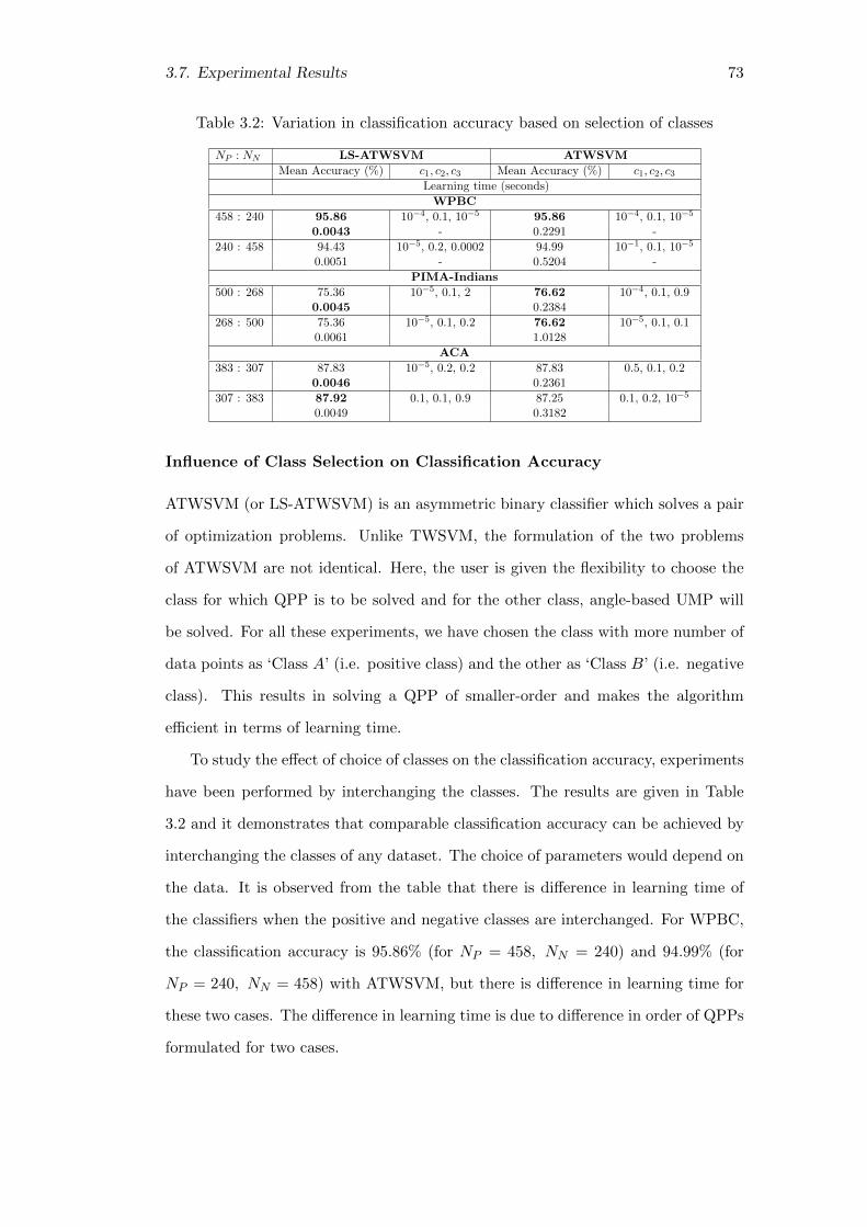
3.7. Experimental Results 73
Table 3.2: Variation in classification accuracy based on selection of classes
NP : NN LS-ATWSVM ATWSVM
Mean Accuracy (%) c1, c2, c3 Mean Accuracy (%) c1, c2, c3
Learning time (seconds)
WPBC
458 : 240 95.86 10−4, 0.1, 10−5 95.86 10−4, 0.1, 10−5
0.0043 - 0.2291 -
240 : 458 94.43 10−5, 0.2, 0.0002 94.99 10−1, 0.1, 10−5
0.0051 - 0.5204 -
PIMA-Indians
500 : 268 75.36 10−5, 0.1, 2 76.62 10−4, 0.1, 0.90.0045 0.2384
268 : 500 75.36 10−5, 0.1, 0.2 76.62 10−5, 0.1, 0.10.0061 1.0128
ACA
383 : 307 87.83 10−5, 0.2, 0.2 87.83 0.5, 0.1, 0.20.0046 0.2361
307 : 383 87.92 0.1, 0.1, 0.9 87.25 0.1, 0.2, 10−5
0.0049 0.3182
Influence of Class Selection on Classification Accuracy
ATWSVM (or LS-ATWSVM) is an asymmetric binary classifier which solves a pair
of optimization problems. Unlike TWSVM, the formulation of the two problems
of ATWSVM are not identical. Here, the user is given the flexibility to choose the
class for which QPP is to be solved and for the other class, angle-based UMP will
be solved. For all these experiments, we have chosen the class with more number of
data points as ‘Class A’ (i.e. positive class) and the other as ‘Class B’ (i.e. negative
class). This results in solving a QPP of smaller-order and makes the algorithm
efficient in terms of learning time.
To study the effect of choice of classes on the classification accuracy, experiments
have been performed by interchanging the classes. The results are given in Table
3.2 and it demonstrates that comparable classification accuracy can be achieved by
interchanging the classes of any dataset. The choice of parameters would depend on
the data. It is observed from the table that there is difference in learning time of
the classifiers when the positive and negative classes are interchanged. For WPBC,
the classification accuracy is 95.86% (for NP = 458, NN = 240) and 94.99% (for
NP = 240, NN = 458) with ATWSVM, but there is difference in learning time for
these two cases. The difference in learning time is due to difference in order of QPPs
formulated for two cases.

74
Tab
le3.
3:C
lass
ifica
tion
resu
lts
wit
hn
on-l
inea
rcl
assi
fier
onb
inar
yU
CI
dat
aset
s
Data
set
TW
SV
MT
PM
SV
MN
HSV
MN
SV
MO
OP
LS-T
WSV
ML
S-A
TW
SV
MA
TW
SV
MA
TP
-SV
M
Mea
nA
ccura
cy(%
)±
SD
AC
A86
.64±
3.61
82.3
2±
3.04
85.7
2±
2.95
79.2
2±
3.46
76.1
7±
5.36
87.2
3±
3.17
87.5
3±
3.17
86.
81±
1.7
4
BU
PA
-Liv
er72
.38±
4.57
73.4
2±
4.24
73.0
9±
6.08
75.7
6±
4.09
74.8
4±
6.85
72.8
9±
4.84
72.
75±
4.84
76.8
6±
4.3
4
Hea
rt-C
84.8
6±
6.55
84.7
7±
3.88
87.2
4±
3.32
84.3
9±
4.54
83.7
9±
5.87
84.8
6±
6.55
84.
92±
6.55
86.
84±
3.1
0
Hea
rt-S
85.3
9±
2.88
85.1
2±
6.06
85.7
3±
4.68
84.5
4±
4.23
85.1
8±
5.23
86.3
0±
2.20
86.
30±
2.20
86.4
8±
4.5
1
Ionos
pher
e91
.23±
3.08
88.4
2±
5.42
89.0
9±
4.68
86.5
2±
4.79
89.6
2±
2.57
92.5
9±
5.25
92.6
1±
5.25
89.
48±
5.6
6
PIM
A-I
ndia
ns
76.2
1±
4.28
77.8
9±
4.28
74.9
7±
4.39
79.0
2±
4.85
75.3
3±
4.67
76.1
6±
2.96
76.
16±
2.96
79.0
4±
6.3
7
Thyro
id92
.18±
4.57
93.4
6±
4.48
93.4
6±
4.48
84.6
0±
8.34
96.2
8±
2.98
95.3
5±
3.11
97.7
1±
3.11
97.7
1±
3.1
1
Tw
onor
m97
.00±
1.21
97.0
0±
1.97
97.7
5±
1.84
97.5
0±
2.04
98.7
5±
1.32
98.0
0±
2.29
97.
25±
2.29
98.
70±
2.0
0
Vot
es96
.05±
2.19
96.7
1±
3.10
97.0
5±
1.50
95.2
9±
3.16
96.1
9±
2.79
96.3
6±
1.96
95.
87±
1.96
96.
51±
2.7
9
WP
BC
96.2
9±
2.15
96.4
2±
1.81
96.0
0±
1.88
96.2
8±
2.04
96.5
6±
2.54
96.4
2±
1.54
96.
71±
1.54
97.1
4±
2.8
6
Mean
Accu
racy
87.8
2±
3.51
87.5
5±
3.83
88.0
1±
3.58
86.3
1±
4.15
87.2
7±
4.02
88.6
2±
3.39
88.
78±
3.39
89.5
6±
3.6
5

3.7. Experimental Results 75
Non-linear Case
For non-linear classifier i.e. RBF kernel Ker(x, x′) = exp(−σ‖x − x′‖22), Table 3.3
presents the classification accuracy for all the above mentioned algorithms on UCI
datasets. The results in the table illustrate that ATP-SVM performs best among
other classifiers and achieves mean accuracy 89.56% over all the 10 UCI datasets. It
is also observed that accuracy obtained with nonlinear kernel is better than the linear
version for corresponding datasets. Taking motivation from Reduced SVM (RSVM)
[64], the experiments have been conducted using ATWSVM with rectangular RBF
kernel Ker(A,A′). A rectangular kernel greatly reduces the size of the problem and
simplifies the generation of non-linear separating surface. For the experiments, we
have used rectangular kernel [64] created using 50% data points which are randomly
selected from the dataset and referred as A.
Classification Results for NDC Datasets
Linear case
In order to study the effect of size of data on the learning time of classifiers, experi-
ments have been conducted on large datasets, generated using David Musicants NDC
Data Generator [53]. Table 3.4 gives the experimental results of ATWSVM, LS-
ATWSVM, LS-TWSVM, TWSVM and ATP-SVM using linear classifiers on NDC
datasets. The distribution of training and test patterns are shown as “Train-Test”
and (NP : NN ) shows the ratio of positive and negative data points. The classifi-
cation accuracy is reported in percent (%) and the results indicate that ATP-SVM
outperforms the other methods for most of the NDC datasets. But ATWSVM,
TWSVM and ATP-SVM fail to generate results for dataset of size 50,000 instances
or more, due to memory constraints of our system. Whereas LS-ATWSVM and
LS-TWSVM perform well for large datasets. This shows that LS-ATWSVM can be
successfully used with low-configuration systems.
Table 3.4 shows the learning time (in seconds) of linear classifiers for NDC
datasets. It is observed that the learning time of ATWSVM is much less as com-
pared to other two classifiers i.e. TWSVM and ATP-SVM, which have comparable
learning time. The experimental results comply with the complexity analysis of

76
Table 3.4: Classification results with linear classifiers on NDC datasets
Dataset Train-Test TWSVM ATP-SVM LS-TWSVM LS-ATWSVM ATWSVM
Mean Accuracy (%)
NDC-500 500-50 84.00 85.00 84.00 85.00 85.00(330 : 170) 0.3172 0.3653 0.0006 0.0005 0.2188
NDC-700 700-70 81.92 85.88 84.29 85.71 85.26(447 : 253) 0.4170 0.4230 0.0007 0.0007 0.2475
NDC-900 900-90 83.45 86.17 85.56 85.56 85.98(571 : 329) 0.5986 0.6160 0.0008 0.0008 0.2859
NDC-1K 1K-100 84.00 85.44 84.00 84.00 85.29(627 : 373) 0.4537 0.4443 0.0008 0.0008 0.2564
NDC-2K 2K-200 84.50 84.75 84.50 86.00 85.00(1246 : 754) 2.1480 2.4649 0.0014 0.0010 0.3805
NDC-3K 3K-300 75.96 78.53 79.40 79.67 79.67(1860 : 1140) 5.3255 5.6775 0.0017 0.0013 0.6161
NDC-4K 4K-400 73.75 75.75 75.03 75.05 75.03(2474 : 1526) 10.5517 10.1186 0.0020 0.0015 0.94
NDC-5K 5K-500 79.78 79.26 78.20 78.56 78.68(3086 : 1914) 10.1965 11.5732 0.0031 0.0020 1.5494
NDC-10K 10K-1K 86.26 86.26 84.50 85.90 85.90(6138 : 3862) 113.8356 102.1345 0.0048 0.0041 6.2377
NDC-50K 50K-5K * * 78.80 79.09 *(30783 : 19217) 0.0274 0.02
NDC-100K 100K-10K * * 85.76 86.11 *(61648 : 38352) 0.0439 0.0371
NDC-200K 200K-20K * * 73.17 74.37 *(122401 : 77599) 0.0877 0.0774
* Experiments terminated due to “out of memory”
these classifiers. Since, ATWSVM solves a QPP and a UMP, the UMP is reduced to
solving a system of linear equations of order (n+ 1) ∗ (n+ 1). Therefore, ATWSVM
requires lesser learning time than TWSVM. For imbalanced datasets, ATWSVM
takes advantage of the distribution of data in the two classes. The hyperplane for
the class with more data points is obtained by solving the QPP, whereas the sec-
ond hyperplane is obtained by solving UMP. Hence, ATWSVM solves the QPP of
smaller order and a UMP whereas TWSVM solves a pair of QPPs. This further
reduces the learning time of ATWSVM. The learning time for LS-ATWSVM and
LS-TWSVM is comparable, but they are more efficient than ATWSVM, TWSVM
and ATP-SVM. This happens because LS-ATWSVM and LS-TWSVM solve systems
of linear equations in feature space and thereby avoids solving QPPs. The compu-
tational efficiency of LS-ATWSVM improves further with the size of dataset and
therefore LS-ATWSVM can be used for experiments with very large-sized datasets,
where TWSVM or TBSVM may fail to give results due to memory constraints or
very high execution time.

3.7. Experimental Results 77
Non-linear Case
The classification accuracy for NDC datasets is reported in Table 3.5 for all clas-
sifiers with Gaussian kernel. The results show that non-linear classifiers achieve
better accuracy than linear classifiers. The table also presents a comparative view
of learning time of all non-linear classifiers for NDC datasets. It is noticed that
LS-ATWSVM is most efficient among all these classifiers.
Table 3.5: Classification result with non-linear classifiers on NDC datasets
Dataset TWSVM ATP-SVM LS-TWSVM LS-ATWSVM ATWSVM
Mean Accuracy (%)Learning time (sec)
NDC-500 84.00 88.00 84.00 88.00 88.000.3018 0.3094 0.0327 0.0306 0.0872
NDC-700 90.00 91.60 90.00 91.43 91.570.3074 0.3086 0.0689 0.0644 0.0951
NDC-900 88.89 89.89 90.00 90.00 90.000.5274 0.5389 0.1378 0.1290 0.1694
NDC-1K 92.00 93.00 92.00 92.50 92.500.6247 0.7381 0.1683 0.1682 0.1928
NDC-2K 91.00 93.00 93.00 91.50 91.503.3214 3.4697 1.0329 0.9142 1.3304
3.7.3 Statistical Tests
To compare the efficacy of multiple classifiers on different datasets, some statis-
tical tools are needed. Since the experiments are conducted with eight classi-
fiers i.e. TWSVM, TPMSVM, NHSVM, NSVMOOP, LS-TWSVM, LS-ATWSVM,
ATWSVM and ATP-SVM, on various UCI datasets, so these are compared by using
Friedman test [54].
Friedman Test
The result for Friedman test on binary classifiers for UCI datasets, regarding classi-
fication accuracy, is given in Table 3.6 and the classifiers ATWSVM and ATP-SVM
achieve the top two ranks among all the approaches. The Friedman test on all eight
algorithms establishes that angle-based classifiers with single optimization problem
achieve better results.

78
Table 3.6: Friedman test ranks with linear classifiers for UCI datasets
Dataset TWSVM TPMSVM NHSVM NSVMOOP LS-TWSVM LS-ATWSVM ATWSVM ATP-SVM
Thyroid 3 7 6 8 4 2 1 5
Heart Statlog 6.5 6.5 6.5 3.5 6.5 3.5 2 1
Heart Cleveland 8 2 6 3 7 5 4 1
Bupa Liver 8 3 6 2 7 4.5 4.5 1
Ionosphere 6 4 3 2 8 7 5 1
Two-norm 5.5 8 5.5 7 1 3.5 3.5 5
Votes 3 8 4 7 5 2 1 6
ACA 5 7 6 8 3.5 1.5 1.5 3.5
WPBC 6 6 2 6 8 3.5 3.5 1
Pima Indians 2 7 8 5 3 4 1 6
Average Rank 5.30 5.85 5.30 5.15 5.3 3.65 2.7 3.05
3.7.4 Multi-category Classification Results: UCI Datasets
This chapter includes extension of NHCs, obtained with single optimization prob-
lem (i.e. ATP-SVM, NSVMOOP and NHSVM) and ATWSVM in multi-category
framework. The extension is done using One-Against-All and Binary Tree based
approaches.
The classification accuracy of NSVMOOP, NHSVM, ATWSVM and ATP-SVM
on multi-category UCI datasets with two approaches- OAA and binary-tree based,
is given in Table 3.7. For each dataset, the number of patterns, features and classes
are shown in the table as m, n and K respectively. The experiments are conducted
with RBF kernel. The classification results show that the ATP-SVM and ATWSVM
can be successfully used as a multi-category classifier and have comparable accuracy
as the other two classifiers i.e. NHSVM and NSVMOOP. It is also observed that
the tree-based approach is better than OAA in terms of classification accuracy.

3.7. Experimental Results 79
Tab
le3.
7:
Cla
ssifi
cati
on
resu
lts
wit
hn
on-l
inea
rcl
assi
fier
onm
ult
i-ca
tego
ryU
CI
data
sets
NH
SV
MN
SV
MO
OP
AT
WSV
MA
TP
-SV
M
OA
AB
TO
AA
BT
OA
AB
TO
AA
BT
Data
set
m×n
(K)
Mea
nA
ccura
cy(%
)±
SD
Der
mat
olog
y36
6×
34(6
)96
.58±
2.18
96.9
7±1.
6096
.97±
3.93
96.9
7±
1.5
997
.34±
2.58
96.6
0±2.7
997
.34±
2.5
898.1
1±
1.99
Eco
li33
6×7
(8)
83.5
8±
5.30
84.3
8±
5.72
85.0
8±7.
2984
.37±
6.5
284
.06±
4.73
85.1
6±4.3
784
.69±
4.1
685.2
9±
5.02
Gla
ss21
4×9
(6)
68.6
4±
9.35
69.1
3±
8.19
71.9
7±
5.14
66.
75±
10.6
070
.29±
3.65
71.6
0±6.1
571
.60±
5.2
871.
88±
5.5
2
Iris
150×
4(3
)94
.67±
6.13
96.0
0±3.
4496
.67±
3.51
95.3
3±
5.4
996
.67±
3.51
97.2
0±2.7
996
.00±
5.6
297.6
7±
2.74
See
ds
210×
7(3
)92
.86±
6.83
94.2
9±4.
3893
.81±
5.52
93.3
3±
7.1
790
.89±
6.51
93.3
3±4.6
590
.95±
6.5
294.7
6±
3.51
Seg
men
t21
0×19
(7)
88.1
0±
5.14
89.5
2±
4.9
287
.62±
7.17
87.6
2±
7.1
788
.10±
5.14
89.1
6±2.7
989
.48±
5.8
589.5
2±
3.69
Win
e17
8×13
(3)
96.6
3±
4.70
97.1
9±
3.96
97.1
9±
5.42
97.7
5±
3.9
297
.19±
3.96
98.1
2±
2.3
696
.63±
3.9
198.3
0±
2.74
Zoo
101×
16(7
)95
.00±
4.72
98.0
0±
4.2
296
.09±
6.91
98.0
0±
4.22
95.0
0±
4.72
98.0
0±
4.2
295
.00±
4.7
298.0
0±
4.22
Mean
Acc.
89.5
1±
5.54
90.6
9±
4.55
90.6
8±
5.61
89.9
7±
5.99
89.9
4±
4.35
91.1
4±3.7
790
.21±
4.83
91.6
9±
3.68

80
Table 3.8: Friedman test and p-values with multi-category classifiers for UCIdatasets
OAA BT OAA BT OAA BT
NHSVM NSVMOOP ATP-SVM
Dataset Rank (p-value) Rank
Derm. 5 (0.1202) 2 (0.1762) 4 (0.1806) 3 (0.4246) 6 (0.4660) 1
Ecoli 6 (0.4680) 4 (0.7072) 5 (0.7255) 2 (0.6541) 3 (0.7722) 1
Glass 5 (0.3568) 4 (0.3906) 6 (0.1916) 1 (0.9707) 3 (0.9081) 2
Iris 6 (0.7169) 3.5 (0.2446) 5 (0.2463) 2 (0.5914) 3.5 (0.1674) 1
Segment 4 (0.4649) 1.5 (0.4855) 5.5 (0.4647) 5.5 (0.4649) 3 (0.9831) 1.5
Seeds 5 (0.4429) 2 (0.7911) 4 (0.5783) 3 (0.6504) 6 (0.1214) 1
Wine 5.5 (0.3458) 3.5 (0.4746) 2 (0.7177) 3.5 (0.5700) 5.5 (0.2838) 1
Zoo 5.5 (0.3823) 2 (1.0000) 2 (1.0000) 4 (0.4655) 5.5 (0.3823) 2
Avg.rank 4.30 2.40 3.45 2.45 3.15 1.05
The multi-category versions of the above mentioned classifiers are compared by
Friedman test in Table 3.8. ATP-SVM achieves the highest rank among all the
approaches. It is also seen that tree-based approach achieves better rank than OAA
multi-category approach. The p-values given in Table 3.8 are tested for a significance
level α = 0.05 and are calculated by pairwise t-test on tree-based ATP-SVM and
other algorithms. Holm-Bonferroni test applied on p-values suggest that ATP-SVM
classifier is similar in performance to TPMSVM, NSVMOOP and NHSVM.
3.8 Application: Segmentation through Pixel Classifi-
cation of Color Images
The problem of image segmentation can be regarded as pixel classification problem
that identifies regions in an image by associating a label with each image pixel. In
this section, we present application of binary and multi-category ATP-SVM to color
image segmentation. For this work, Gabor texture features [65] are determined for
each pixel of the image.
Segmentation: Object and Background
In this thesis, we have explored the application of angle-based classifiers for color
pixel classification problem which can partition the image into two regions corre-
sponding to object and background. Since ATP-SVM and ATWSVM are binary
classifiers, they can be trained to associate the image pixels to some homogeneous

3.8. Application: Segmentation through Pixel Classification of Color Images 81
region that either belongs to the object or to the background. The RGB image is first
quantized with minimum variance color quantization for two levels. The training set
consists of 1% randomly selected pixels and the pixel labels are given by correspond-
ing quantized color value. Gabor features [56] with 4-orientation (0, 45, 90, 135) and
3-scale (0.5, 1.0, 2.0) sub-bands and the maximum of the 12 coefficients determine
the orientation at a given pixel location. These features are used as input to the
classifiers which determine labels for all pixels. It takes advantage of the local infor-
mation of color image and uses the ability of our classifier to distinguish the object
pixels from background.
Table 3.9: Segmentation results for BSD color images
Segmentation (2-regions)
Image L F-measure Error rate
K-Means ATP-SVM K-Means ATP-SVM
42049 2 0.84 0.91 0.0346 0.0267
35049 2 0.57 0.59 0.0479 0.0395
296059 2 0.67 0.77 0.0408 0.0304
181021 2 0.59 0.63 0.0406 0.0385
196027 2 0.51 0.58 0.0874 0.0640
Segmentation (multi-region)
118035 4 0.63 0.75 0.0411 0.0232
100007 3 0.58 0.63 0.0445 0.0323
163014 4 0.44 0.60 0.0833 0.0598
124084 4 0.60 0.61 0.0536 0.0473
196027 4 0.45 0.56 0.0751 0.0344
This section presents the segmentation results of color images selected from
Berkley Segmentation Dataset (BSD) [57]. For BSD images, the ground truth seg-
mentations are known and the images segmented by ATP-SVM are compared with
ground truth. To evaluate the segmentation algorithms statistically, two criteria are
used: F-measure (FM) and error rate (ER). (Please refer Appendix A for details.)
Experiments show that the classifier ATP-SVM can generate effective image seg-
mentation results and is able to distinguish the object from the background. To
compare the segmentation results, we have implemented pixel classification through
K-Means clustering [25]. It is observed from Table 3.9 that ATP-SVM achieves bet-
ter F-measure and error rate values. This is validated by the image segmentation
results given in Table 3.10. With K-Means, many object pixels are misclassified
as background pixels. The segmentation results are visually more appealing for

82
ATP-SVM.
It is observed from Table 3.11 that ATWSVM is able to achieve better re-
sults than segmentation with K-Means clustering. The segmentation results for
ATWSVM are visibly more satisfactory as compared to other method and the same
is proved by F-measure and error rate. The segmentation results are given in Table
3.12.
Segmentation: Multiple Regions
ATP-SVM can be used to identify multiple non-overlapping regions in an image in
multi-category framework. A dynamic method is used to determine the number of
regions in each image by generating its histogram and identifying the prominent
peaks. The number of prominent peaks determine the number of regions (L) in the
image. The image is then color quantized using minimum variance quantization for
L levels and each pixel gets associated with some color value. The training and
test data is created in the similar manner as for binary segmentation and the multi-
category classifier model is build using the training data. For this chapter, binary-
tree based multi-category approach is used. The multi-region segmentation achieved
by ATP-SVM is compared with segmentation obtained by K-Means clustering [25]
and Normalized cut (Ncut) [66]. The results are presented in Table 3.9 (Multi-
region results) and Table 3.13 and it is observed that Ncut is not able to produce
satisfactory output.
3.9 Conclusions
In this chapter, two novel classifiers are presented. The first classifier is Angle-based
Twin Parametric-Margin Support Vector Machine (ATP-SVM) which solves only
one quadratic programming problem for simultaneously determining two parametric-
margin hyperplanes and is particularly useful when the data has heteroscedastic
noise. It tries to maximize the angle between the two hyperplanes and avoids the
explicit computation of inverse of matrices in the dual. Also, a novel procedure for
selecting the ‘data representative points’ is presented, which can effectively reduce
the size of training set and hence reduces the complexity of the problem. Thus,

3.9. Conclusions 83
42049
35049
296059
181021
196027
Image No. (a.) Original image (b.) Image segmented (c.) Image segmentedwith K-Means with ATP-SVM
Table 3.10: Segmentation results (binary) on color images from BSD image dataset

84
118035
42049
124084
135069
299091
Image No. (a.) Original image (b.) Image segmented (c.) Image segmentedwith K-Means with ATWSVM
Table 3.11: Segmentation results (binary) on color images from BSD image dataset
our classifier is able to attain the speed comparable to that of TWSVM and results
in faster execution than any other single optimization based classifier. Further,
multi-category ATP-SVM using One-Against-One (OAA) and Binary Tree (BT)
approaches are presented, along with the application for segmentation of color images
into two or more regions.
The second classifier is Angle-based Twin Support Vector Machine (ATWSVM)
which determines the two hyperplanes by solving a quadratic programming problem
and an unconstrained minimization problem. The first problem of ATWSVM can
be formulated as any TWSVM-based optimization problem and obtains positive
hyperplane. The second problem obtains the hyperplane so that it is proximal to the
data points of its own class and is at maximum angle from the positive hyperplane.
ATWSVM classifier has efficient time-complexity than TWSVM and TBSVM, since

3.9. Conclusions 85
Table 3.12: Segmentation result for BSD color images
Image ATWSVM K-Means
F-measure Error rate F-measure Error rate
299091 0.77 0.0083 0.42 0.0323
135069 0.94 0.0169 0.60 0.0500
118035 0.71 0.0382 0.70 0.0416
42049 0.91 0.0298 0.82 0.0344
124084 0.61 0.0722 0.42 0.1245
the second problem of ATWSVM avoids solving QPP. This research work presents
a generic model for binary classifiers where the first problem can be solved using
any TWSVM-based classifier like ITWSVM [61], TPMSVM [16] or LS-TWSVM
[14] and the second problem would remain the same. The efficacy of ATWSVM has
been proved by performing experiments with synthetic and real world datasets and
ATWSVM is further applied for color image segmentation.

86
118035
100007
163014
124084
124084
BSD No. (a.) Original image (b.) Ncut* (c.) K-Means (d.) ATP-SVM
* Code source:https://in.mathworks.com/matlabcentral/fileexchange/52698-K-Means–mean-shift-and-normalized-cut-segmentation?requestedDomain=www.mathworks.com.
Table 3.13: Segmentation results (multi-region) with normalized cut, K-Means andATP-SVM on color images of BSD dataset

Chapter 4
Ternary Support Vector Machine with
Extension for Multi-category Classification
4.1 Introduction
In this chapter, we present a ternary (i.e. three class) classifier termed as Ternary
Support Vector Machine (TerSVM) and its extension for multi-category classifica-
tion. The motivation behind this chapter is to develop an algorithm which can
efficiently handle multi-class data. The existing multi-category classification ap-
proaches like One-Against-All (OAA) and One-Against-One (OAO) are not efficient
in terms of learning time. Their performance deteriorates with increase in number
of classes. So, we present a tree-based multi-category algorithm which is robust
enough to deal with large number of classes and is termed as Reduced Tree for
Ternary Support Vector Machine (RT-TerSVM).
TerSVM is developed on the lines of Twin-KSVC [39] and evaluates the training
data into ‘one-versus-one-versus-rest’ structure. But the problem formulation of
TerSVM is quite different from that of Twin-KSVC. The significant features of our
classifier TerSVM are listed below:
1. The supervised classification algorithm i.e. TerSVM, is a ternary classifier
which deals with three classes: positive, negative and rest, associated with
labels +1, −1 and 0 respectively. If required, TerSVM can be used as binary
classifier also.
2. TerSVM formulates three unconstrained minimization problems (UMPs) to
determine proximal hyperplanes for three classes. These optimization prob-

88
lems are solved as systems of linear equations, whereas Twin-KSVC solves
quadratic programming problems (QPPs).
3. Our classifier optimizes the distance (i.e. ρ1, ρ2) between the hyperplane of one
class and patterns of the other class, whereas Twin-KSVC tries to maintain a
separation of unit distance.
4. TerSVM first solves the optimization problems for positive and negative classes.
Then the hyperplane for the rest class is determined by using the solution of
the other two problems.
This chapter also presents a novel multi-category classification approach and its
characteristic features are listed below.
1. The novel approach i.e. RT-TerSVM, is a tree-based multi-category classifi-
cation algorithm that evaluates the training data into ‘one-versus-one-versus-
rest’ structure. RT-TerSVM identifies the two most distant classes as positive
and negative classes. The remaining classes are collectively referred as rest
class and their patterns are mapped in the region between positive and nega-
tive classes. RT-TerSVM recursively divides the data of ‘rest’ class further into
three classes in the similar manner until all the classes are uniquely represented
in the ternary tree.
2. This work presents an effective procedure to identify positive, negative and
rest classes from a given set of K classes, such that the rest class is mapped
between positive and negative classes.
3. At each level, RT-TerSVM determines three nonparallel hyperplanes using
TerSVM classifier and evaluates the test data based on minimum distance
from these hyperplanes.
4. Each leaf node of the RT-TerSVM is associated with a unique class and the
internal nodes are employed to distinguish between these classes.
5. RT-TerSVM develops a ternary tree of height bK/2c, where K is the number
of classes in the dataset. The size of the problem reduces as we traverse down
the ternary tree and this results in efficient learning time.

4.2. Ternary Support Vector Machine 89
6. To improve the learning time complexity of our algorithm, we present a novel
procedure to generate a reduced training set which can effectively represent
the entire training set.
The remaining chapter is organized as follows: Sections 4.2 and 4.3 present the
novel classifier Ternary Support Vector Machine (TerSVM) and the multi-category
extension approach. Section 4.4 compares TerSVM with other multi-category algo-
rithms. The experimental results on synthetic and benchmark datasets are given in
Section 4.5. This chapters also presents the application of RT-TerSVM for handwrit-
ten digit recognition and color image classification in Section 4.6. The concluding
remarks are given in Section 4.7.
4.2 Ternary Support Vector Machine
In this section, we introduce a TWSVM-based classifier which can handle three
classes and is therefore termed as Ternary Support Vector Machine (TerSVM).
TWSVM and most of its variants solve QPPs to obtain the nonparallel hyperplanes.
Kumar at al. proposed a faster version of TWSVM as Least Squares TWSVM (LS-
TWSVM) [14] which solves systems of linear equations to generate the proximal
hyperplanes. Taking motivation from LS-TWSVM, TerSVM obtains classifiers by
solving systems of linear equations. Let the three classes are represented by matrices
A (m1×n), B (m2×n) and C (m3×n) which are referred as positive (+1), negative
(−1) and rest (0) classes. The dataset X = [A; B; C] has m = m1 +m2 +m3 pat-
terns. This classifier determines three proximal nonparallel hyperplanes by solving
unconstrained minimization problems (UMPs). The three hyperplanes are given by
xTw1 + b1 = 0,
xTw2 + b2 = 0,
xTw3 + b3 = 0, (4.1)
where (w1, b1), (w2, b2) and (w2, b2) are the parameters of normal vectors to the
positive, negative and rest hyperplanes.

90
4.2.1 TerSVM (Linear version)
The TerSVM hyperplanes for three classes (i.e. A, B and C) are obtained by solving
the following three optimization problems:
TerSVM1:
minw1,b1,ρ1,ξ1,η1
PA =1
2‖Aw1 + e1b1‖22 +
c1
2ξT1 ξ1 +
c2
2ηT1 η1 +
c3
2ρT1 ρ1
subject to −(Bw1 + e2b1) + ξ1 = e2(1− ρ1),
−(Cw1 + e3b1) + η1 = e3(1− ε− ρ1). (4.2)
TerSVM2:
minw2,b2,ρ2,ξ2,η2
PB =1
2‖Bw2 + e2b2‖22 +
c1
2ξT2 ξ2 +
c2
2ηT2 η2 +
c3
2ρT2 ρ2
subject to (Aw2 + e1b2) + ξ2 = e1(1− ρ2),
(Cw2 + e3b2) + η2 = e3(1− ε− ρ2). (4.3)
TerSVM3:
minw3,b3,ξ3,η3
PC =1
2‖Cw3 + e3b3‖22 +
c1
2ξT3 ξ3 +
c1
2ηT3 η3 +
c4
2
(w1
Tw3 + w2Tw3 + b1b3 + b2b3
)subject to (Aw3 + e1b3) + ξ3 = e1(1− ε− ρ1),
−(Bw3 + e2b3) + η3 = e2(1− ε− ρ2). (4.4)
TerSVM1: The TerSVM classifier assumes that the rest class is placed between
positive and negative classes. The optimization problem given in (4.2) determines
the parameters of positive hyperplane (w1, b1), which is proximal to the positive
class (represented by A). The term 12‖Aw1 +e1b1‖22 in the objective function of (4.2)
is the sum of squared distances of the positive hyperplane to the patterns of its own
class. Thus, minimizing this term tends to keep the hyperplane closer to the positive
class. The equality constraints require that the negative class patterns (represented
by B) should be exactly (1− ρ1) distance away from the positive hyperplane. Since
TerSVM is soft-margin classifier, it allows some error in classification. The amount

4.2. Ternary Support Vector Machine 91
of violation of constraints is measured by ξ1 and its L2-norm is minimized in the
objective function. This is in contrast to Twin-KSVC problem which minimizes the
L1-norm of error vector and has inequality constraints. Similarly, the other set of
constraints require the patterns of rest class to be (1 − ε − ρ1) distance away from
the positive hyperplane. The error due to misclassification of patterns of rest class
is measured by η1 and is minimized in (4.2). To have maximum separation between
patterns of one class and hyperplane of other class, the distance ρ1 is minimized in
our problem and ε is user-defined parameter. The positive parameters ci, i = 1, .., 4
associate weights with the corresponding terms.
The optimization problem (4.2) is converted into an unconstrained minimization
problem (UMP) by substituting ξ1, η1 and we get
minw1,b1,ρ1
PA =1
2‖Aw1 + e1b1‖22 +
c1
2‖Bw1 + e2b1 + e2(1− ρ1)‖22 +
c2
2‖Cw1 + e3b1 + e3(1− ε− ρ1)‖22 +
c3
2ρT1 ρ1. (4.5)
The second and third terms of the objective function of (4.5) try to minimize the
L2-norm of the error due to misclassified patterns of negative and rest classes re-
spectively, with parameters c1 and c2. Taking sub-gradient of PA with respect to
w1, b1, ρ1 and equating them to zero, we get
∂PA∂w1
= 0⇒ AT (Aw1 + e1b1) + c1BT (Bw1 + e2b1 + e2(1− ρ1)) +
c2CT (Cw1 + e3b1 + e3(1− ε− ρ1)) = 0, (4.6)
∂PA∂b1
= 0⇒ eT1 (Aw1 + e1b1) + c1eT2 (Bw1 + e2b1 + e2(1− ρ1)) +
c2eT3 (Cw1 + e3b1 + e3(1− ε− ρ1)) = 0, (4.7)
∂PA∂ρ1
= 0⇒ −c1eT2 (Bw1 + e2b1 + e2(1− ρ1)) +
−c2eT3 (Cw1 + e3b1 + e3(1− ε− ρ1)) + c3ρ1 = 0. (4.8)
Let H = [A e1], G = [B e2], J = [C e3] be the augmented matrices for positive,
negative and rest classes respectively. The normal vector to the hyperplane is repre-
sented by augmented vector z1 = [wT1 bT1 ]T , which includes the bias term b1; e1, e2
and e3 are vectors of ones of appropriate dimensions. The above equations (4.6-4.8)
could be rewritten as

92
HTHz1 + c1GT (Gz1 + e2(1− ρ1)) + c2J
T (Jz1 + e3(1− ε− ρ1)) = 0, (4.9)
−c1eT2 (Gz1 + e2(1− ρ1))− c2e
T3 (Jz1 + e3(1− ε− ρ1)) + c3ρ1 = 0, (4.10)
Arranging Eq.(4.9) and (4.10) in matrix form, we get
HTH + c1GTG+ c2J
TJ −c1GT e2 − c2J
T e3
−c1eT2 G− c2e
T3 J c1e
T2 e2 + c2e
T3 e3 + c3
z1
ρ1
=
−c1GT e2 − c2J
T e3(1− ε)
c1eT2 e2 + c2e
T3 e3(1− ε)
(4.11)
The augmented vector z1 and distance ρ1 are obtained as
z1
ρ1
=
HTH + c1GTG+ c2J
TJ −c1GT e2 − c2J
T e3
−c1eT2 G− c2e
T3 J c1e
T2 e2 + c2e
T3 e3 + c3
−1
−c1GT e2 − c2J
T e3(1− ε)
c1eT2 e2 + c2e
T3 e3(1− ε)
. (4.12)
TerSVM2: The optimization problem (4.3) for determining negative hyperplane is
analogous to the first QPP and is converted into UMP given by
minw2,b2,ρ2
PB =1
2‖Bw2 + e2b2‖22 +
c1
2‖Aw2 + e1b2 − e2(1− ρ2)‖22 +
c2
2‖Cw2 + e3b2 − e3(1− ε− ρ2)‖22 +
c3
2ρT2 ρ2. (4.13)
The solution of the above equation is obtained as
z2
ρ2
=
GTG+ c1HTH + c2J
TJ c1HT e1 + c2J
T e3
c1eT1 H + c2e
T3 J c1e
T1 e1 + c2e
T3 e3 + c3
−1
c1HT e1 + c2J
T e3(1− ε)
c1eT1 e1 + c2e
T3 e3(1− ε)
, (4.14)

4.2. Ternary Support Vector Machine 93
where z2 = [wT2 bT2 ]T is the augmented vector for negative hyperplane.
Figure 4.1: Geometrical illustration of angle between normal vectors to the hyper-planes
TerSVM3: The problem (4.4) is different from the first two problems and uses
the solution of TerSVM1 and TerSVM2. It requires the optimal values of positive
(w1, b1) and negative (w2, b2) hyperplanes along with optimal values of ρ1 and
ρ2. The proximal hyperplane is determined so that it is (1− ε− ρ1) distance away
from the patterns of positive class and (1− ε− ρ2) distance away from the patterns
of negative class. The objective function of TerSVM3 tries to maximize the angle
between the normal vector to rest hyperplane and the normal vectors to the other
two hyperplanes, as shown in Figure 4.1. Since,
cos θ1 =(w0.w1)
‖w0‖2‖w1‖2and cos θ2 =
(w0.w2)
‖w0‖2‖w2‖2,
the cosine of angle θ1 and θ2 could be minimized to achieve the maximum separation
between the hyperplanes. The optimization problem of (4.4) is converted into UMP
given as
minw3,b3
PC =1
2‖Cw3 + e3b3‖22 +
c1
2‖Aw3 + e1b3 − e1(1− ε− ρ1)‖22 +
c1
2‖Bw3 + e2b3 + e2(1− ε− ρ2)‖22 +
c4(w1Tw3 + w2
Tw3 + b1.b3 + b2.b3). (4.15)

94
The last term of (4.15) tries to simultaneously maximize the angle between the opti-
mal positive w1 and the rest w3 hyperplane (represented by w1Tw3) and also between
negative w2 hyperplanes and rest w3 hyperplane (represented by w2Tw3). To obtain
the hyperplane corresponding to the rest class, the optimal solution (i.e. z1, z2, ρ1
and ρ1) of TerSVM1 and TerSVM2 are used. The solution for rest hyperplane is
obtained by solving
[z3
]=
[JTJ + c1H
TH + c2GTG
]−1
[c1
(HT e1(1− ε− ρ1)−GT e2(1− ε− ρ2)
)− c4(z1 + z2)
], (4.16)
where z3 = [wT3 bT3 ]T is the augmented vector for rest hyperplane. A new test
pattern x ∈ Rn is assigned to class r (r = +1,−1, 0), based on minimum distance
from the three hyperplanes. The class label is given by
y = arg
(minl=1,2,3
|xTwl + bl|‖wl‖2
), (4.17)
where |.| is the absolute distance of point x from the plane xTwl + bl = 0 and ‖.‖2
represents L2-norm. The label assigned to the test data is given as
y =
+1 (r = 1)
−1 (r = 2)
0 (r = 3)
.
4.2.2 TerSVM (Kernel version)
This classifier can be extended to non-linear version by considering the kernel-
generated surfaces instead of hyperplanes. The surfaces are given as
Ker(xT , (X )T )u1 + b1 = 0, (4.18)
Ker(xT , (X )T )u2 + b2 = 0, (4.19)
Ker(xT , (X )T )u3 + b3 = 0, (4.20)

4.2. Ternary Support Vector Machine 95
where X = [A; B; C] represents the entire dataset and Ker is an appropriately
chosen kernel. The formulation of kernel TerSVM is given as
minu1,b1,ρ1
1
2‖Ker(A,X T )u1 + e1b1‖22 +
c1
2‖Ker(B,X T )u1 + e2b1 + e2(1− ρ1)‖22 +
c2
2‖Ker(C,X T )u1 + e3b1 + e3(1− ε− ρ1)‖22 +
c3
2ρT1 ρ1. (4.21)
minu2,b2,ρ2
1
2‖Ker(B,X T )u2 + e2b2‖22 +
c1
2‖Ker(A,X T )u2 + e1b2 − e2(1− ρ2)‖22 +
c2
2‖Ker(C,X T )u2 + e3b2 − e3(1− ε− ρ2)‖22 +
c3
2ρT2 ρ2. (4.22)
minu3,b3
1
2‖Ker(C,X T )u3 + e3b3‖22 +
c1
2‖Ker(A,X T )u3 + e1b3 − e1(1− ε− ρ1)‖22 +
c1
2‖Ker(B,X T )u3 + e2b3 + e2(1− ε− ρ2)‖22 +
c4(w1Tu3 + w2
Tw3 + b1.b3 + b2.b3), (4.23)
where Ker(A,X T ), Ker(B,X T ), Ker(C,X T ) represent kernel matrices for classes
A, B and C respectively. The solutions for these problems are obtained in similar
manner as for linear case. The augmented vector for positive hyperplane r1 =
[uT1 bT1 ] is given as
r1
ρ1
=
HTKHK + c1G
TKGK + c2J
TKJK −c1G
TKe2 − c2J
TKe3
−c1eT2 GK − c2e
T3 JK c1e
T2 e2 + c2e
T3 e3 + c3
−1
−c1GTKe2 − c2J
TKe3(1− ε)
c1eT2 e2 + c2e
T3 e3(1− ε)
. (4.24)
Here, HK = [Ker(A,X e1], GK = [Ker(B,X e2], JK = [Ker(C,X e3]; e1, e2
and e3 are vectors of ones of appropriate dimensions. The solution for the negative
hyperplane is given as
r2
ρ2
=
GTKGK + c1HTKHK + c2J
TKJK c1H
TKe1 + c2J
TKe3
c1eT1 HK + c2e
T3 JK c1e
T1 e1 + c2e
T3 e3 + c3
−1
c1HTKe1 + c2J
TKe3(1− ε)
c1eT1 e1 + c2e
T3 e3(1− ε)
, (4.25)

96
where r2 = [uT2 bT2 ]T is the augmented vector for negative hyperplane. The solution
for rest hyperplane r3 = [uT3 bT3 ]T is obtained by solving
[r3
]=
[JTKJK + c1H
TKHK + c2G
TKGK
]−1
[c1(HT
Ke1(1− ε− ρ1)−GTKe2(1− ε− ρ2))− c4(r1 + r2)
]. (4.26)
Once we obtain the surfaces (4.18), a new pattern x ∈ Rn is assigned to class 1, -1
or 0 in a manner similar to the linear case.
4.2.3 TerSVM as Binary Classifier
The ternary classifier can also be used as a binary classifier. For a two-class classifi-
cation problem, there would be no rest class and only two nonparallel hyperplanes
are determined corresponding to positive and negative classes. The optimization
problems for binary TerSVM are:
minw1,b1,ρ1
PA =1
2‖Aw1 + e1b1‖22 +
c1
2‖Bw1 + e2b1 + e2(1− ρ1)‖22 +
c3
2ρT1 ρ1, (4.27)
minw2,b2,ρ2
PB =1
2‖Bw2 + e2b2‖22 +
c1
2‖Aw2 + e1b2 − e2(1− ρ2)‖22 +
c3
2ρT2 ρ2. (4.28)
The equations (4.27) and (4.28) are UMPs which can be solved in similar manner
as (4.5).
4.3 Multi-category Classification Algorithm: Reduced
Tree for TerSVM
In this section, we present a novel multi-category classification approach which can
efficiently handle large amount of data from more than two classes. The multi-
category classification approach is motivated by Twin-KSVC [39] and implements
a ternary tree (i.e. a tree where each node can have at most three child nodes)
of classifiers to organize multiple classes. This algorithm recursively partitions the

4.3. Multi-category Classification Algorithm: Reduced Tree for TerSVM 97
Figure 4.2: RT-TerSVM for dataset with 5 classes
set of K classes into one positive class, one negative class and remaining (or rest)
classes denoted by +1, −1 and 0 respectively. The remaining (K − 2) classes are
recursively partitioned until all the classes are uniquely represented by a leaf node of
the ternary tree, as demonstrated in Figure 4.2. Once the hyperplanes are obtained
for the positive and negative classes, their patterns are removed from the training
set. Therefore, to determine the hyperplanes for remaining (K − 2) classes, these
2 classes (i.e. positive and negative classes in higher level of the tree) are not
considered. This reduces the number of training samples and hence, the learning
time of the algorithm. Our algorithm achieves good classification accuracy, which is
proved experimentally in Section 4.5. To identify the positive and negative classes
at each level of the RT-TerSVM, a novel class selection approach is presented in

98
Algorithm 2.
Input : Training data X = X1, X2, ..., Xm with labels y ∈ 1, 2, ...,K.
Output : Positive, negative and rest classes.
Process:
1. For each class Ci, i = 1, ...,K, identify
a. class mean Mi.
b. span of each class (Spani) where span is given as
Spani =1
mi
mi∑j=1
‖Xj −Mi‖2, (4.29)
where mi is the number of patterns in ith class and ‖Xj −Mi‖2 is the
Euclidean distance between data pattern Xj and class mean Mi.
2. For p=1 to K
For q=p+1 to K
Find the separation between classes Cp and Cq, given by
D(Cp, Cq) = ‖Mp −Mq‖2 − Spanp − Spanq. (4.30)
End.
End.
3. Select the classes i, j as positive and negative classes respectively, such
that the distance D(Ci, Cj) is maximum.
4. The remaining classes of the dataset i.e. Cr, r ∈ K − i, j are treated
as rest class and would lie in the region between the positive and negative
classes.Algorithm 2: Selection of positive, negative and rest classes
Reduced training set
To improve the learning time of our algorithm, we present a novel procedure that
selects a subset of training patterns which is referred as reduced training set. For
our multi-category classification algorithm, a ternary tree is built by first selecting
positive, negative and rest classes. Since the number of patterns in rest class would
be more than those in other two classes, a selection procedure in Algorithm 3 is

4.3. Multi-category Classification Algorithm: Reduced Tree for TerSVM 99
presented which can identify few representative patterns from the rest class. The
reduced patterns can effectively represent the entire training set and it is exper-
imentally observed that we can achieve good classification accuracy with reduced
training set. It significantly improves the learning time of our algorithm.
Input : Training data X = X1, X2, ..., Xm with labels y ∈ +1,−1, 0.
Output : Reduced training set.
Process:
1. Calculate class mean M0 for rest class.
2. For each pattern in rest class, find its distance from M0.
disti = ‖Xi −M0‖, (4.31)
where ‖Xi −M0‖ is the Euclidean distance.
2. Select P% patterns which are most distant from the class mean M0.
Algorithm 3: Procedure to create reduced training set
Reduced tree for Ternary Support Vector Machine (RT-TerSVM)
RT-TerSVM is a supervised learning approach that builds a classifier model for K
classes by using m training points. The procedure for generating RT-TerSVM is
explained in Algorithm 4. The inputs to the algorithm are X ∈ Rm×n and K, where
X represents m data points in n-dimensional feature space and K is the number of
classes. The multi-category classification approach i.e. RT-TerSVM identifies two
classes as positive and negative and remaining all training patterns as taken as rest
class. For a dataset with K classes, the +1 and −1 classes are identified based on
maximum distance between them, using Algorithm 2. The remaining K − 2 classes
are treated as rest class. The patterns in the rest class are recursively partitioned
until each class is uniquely represented in the classifier model. RT-TerSVM develops
a ternary tree of height bK/2c, where K is the number of classes in the dataset. At
each level, RT-TerSVM obtains three nonparallel hyperplanes and evaluates the test
data based on minimum distance from these hyperplanes. Each leaf node of the
RT-TerSVM is associated with a unique class and the internal nodes are employed
to distinguish between these classes. The size of the problem reduces as we traverse
down the ternary tree and this results in efficient learning time. This approach

100
performs better that the classical One-Against-All (OAA), Twin-KSVC and other
tree-based multi-category approaches, in terms of generalization ability and learning
time. A test pattern xi ∈ Rn is evaluated using the trained RT-TerSVM model and
the procedure is explained in Algorithm 5.
4.4 Discussion
The strength of our multi-category approach RT-TerSVM is its efficient training and
testing time. RT-TerSVM evolves as a recursive classifier model with better time
complexity as compared to classical One-Against-All approach. The size of data
diminishes as the model is progressively obtained. This characteristic favors the use
of non-linear (kernel) classifiers where the learning time depends on the size of data.
Input : Labeled dataset with m patterns from K different classes.
Output : The hyperplane parameters for all internal and leaf nodes that
build up the RT-TerSVM.
Process: RT-TerSVM(X ,K)
1. Use Algorithm 2 to identify positive, negative and rest classes with labels
‘+1’, ‘-1’ and ’0’ respectively. The two most distant classes are referred as
A, B, and remaining classes as C.
2. Take training patterns of ‘+1’, ‘-1’ and ‘0’ classes and find three
hyperplanes [w1, b1], [w2, b2] and [w3, b3] by solving (4.12, 4.14, 4.16) or
using the kernel based versions of TerSVM classifier (4.21-4.23).
3. If the number of classes in C are more than one, then recursively call this
algorithm: RT-TerSVM(Xnew, K − 2),
where Xnew = X − A,B.Algorithm 4: Reduced Tree for Ternary Support Vector Machine
Twin-KSVC: For a K-class problem, Twin-KSVC formulates K∗(K−1)2 prob-
lems. Each problem determine two nonparallel hyperplanes and uses the entire
dataset. Assume that all classes have approximately equal number of patterns i.e.
m/K, where m is the total number of data points. The learning time of one Twin-
KSVC problem is of the order
2×(K − 1
K∗m
)3
. (4.32)

4.4. Discussion 101
Since, twin-KSVC solves K∗(K−1)2 problems, its total learning time is of the order
2×(K − 1
K∗m
)3
× K ∗ (K − 1)
2,
⇒ (K − 1)4
K2m3 (4.33)
u K2 ×m3. (4.34)
Therefore, the learning time of Twin-KSVC increases with the number of classes.
OAA-TWSVM: When TWSVM binary classifier is extended in multi-category
framework using OAA approach, then the algorithm solves K QPPs, each of size
((K − 1)/K) ∗m. Hence, the learning time of OAA-TWSVM is given by
TOAA = K ∗(K−1K ∗m
)3,
u K ∗m3. (4.35)
TerSVM-Tree: Our multi-category algorithm uses a ternary classifier TerSVM,
which solves the optimization problems as systems of linear equation. For the linear
case, TerSVM solves three problems where two of them find the inverse of matrix
of order (n + 2) × (n + 2) and one problem finds the inverse of matrix of order
(n+ 1)× (n+ 1). Here, n is the number of features. The data from the rest class is
further partitioned and time complexity of RT-TerSVM is given as
T (m) = [2(n+ 2)3 + (n+ 1)3] + [2(n+ 2)3 + (n+ 1)3] + ....
(bK
2c- terms
)=
(bK
2c)× [2(n+ 2)3 + (n+ 1)3]
u K × n3. (4.36)
The height of the ternary tree is bK2 c. Since n << m, therefore, the learning time
of linear RT-TerSVM is much less than that of Twin-KSVC or OAA-TWSVM.
For kernel version, RT-TerSVM determines inverse of matrices of order (m+2)×
(m+ 2) and avoids solving QPPs, as solved by the other two approaches. Our algo-
rithm uses reduced training set which further improves its learning time. Therefore,
TerSVM outperforms Twin-KSVC and OAA-TWSVM in terms of learning time.

102
Input : The hyperplane parameters for all internal and leaf nodes thatbuild up the RT-TerSVM; Test pattern xi.
Output : Label for test pattern.Process:1. The test pattern xi is evaluated at the root node where the distance fromthree hyperplanes i.e. +1, −1 and 0, is determined, using Eq.(4.17).
2. Repeata. The pattern xi is associated with the class whose hyperplane is at the
minimum distance from the pattern.b. If the associated class is +1 or −1,
i. then assign the actual label of that class to xi.ii. break.else if number of classes in rest class is one
i. then assign the actual label of that class.ii. break.elsei. Determine the distance of pattern xi from the three
hyperplanes at next level of the RT-TerSVM.3. End.
Algorithm 5: Testing a data pattern using RT-TerSVM.
RT-TerSVM vs. Twin-KSVC
Both RT-TerSVM and Twin-KSVC extend nonparallel hyperplanes classifiers into
multi-category framework by evaluating training points into ‘one-versus-one-versus-
rest’ structure. For a K-class classification problem, Twin-KSVC constructs K(K−
1)/2 classifiers, where each classifier solves two QPPs. Whereas for RT-TerSVM,
bK/2c classifiers are constructed and each TerSVM classifier solves three UMPs.
The testing time for Twin-KSVC is more than RT-TerSVM, due to large number
of classifiers and the final label depends on the voting decision rules. But for RT-
TerSVM, pattern testing is based on minimum distance from the three TerSVM
hyperplanes. Therefore, maximum testing time depends on the height of the tree,
which is much less than the number of classifiers obtained for Twin-KSVC.
RT-TerSVM is time efficient than Twin-KSVC because it formulates the op-
timization problems as UMPs, rather than QPPs. The solution is obtained, for
TerSVM, by solving a system of linear equations. This makes our algorithm feasible
for real life large-sized problems. Twin-KSVC considers unit distance separability
between positive-hyperplane and patterns of other classes and vice-versa. Whereas
RT-TerSVM optimizes the separating distance (ρ1 and ρ2) between patterns of one
class and hyperplane of other class. Figure 4.3 graphically illustrates the hyper-

4.4. Discussion 103
planes obtained by TerSVM and Twin-KSVC classifiers. For a three-class problem,
TerSVM solves three UMPs to obtain proximal hyperplanes; whereas, Twin-KSVC
builds classifiers as 1-vs-2-vs-rest, 2-vs-3-vs-rest, 3-vs-1-vs-rest.
(a) TerSVM: Three hyperplanes obtained by TerSVM classifier
(b) Twin-KSVC: Hyperplanes are obtained as 1-vs-2-vs-rest, 2-vs-3-vs-rest, 3-vs-1-vs-rest
Figure 4.3: Synthetic dataset with 300 data points. Hyperplanes obtained by a.TerSVM; b. Twin-KSVC
RT-TerSVM vs. TDS-TWSVM
Ternary Decision Structure (TDS) is a multi-category classification algorithm that
generates the classifier model in a hierarchical manner. It partitions the training data
into at most three groups and is discussed in more detail in Section 5.2. TDS evalu-

104
ates the training patterns using ‘i-versus-j-versus-k’ structure whereas RT-TerSVM
uses ‘one-versus-one-versus-rest’ structure. TDS extends an existing binary classifier
like TWSVM into multi-category framework. It uses K-Means clustering to iden-
tify three groups of classes and generates their proximal hyperplanes using OAA
method for three classes.RT-TerSVM and TDS-TWSVM are multi-category classi-
fication algorithms for nonparallel hyperplanes classifiers; but their approaches are
totally different.
In contrast, RT-TerSVM is built upon a novel ternary classifier i.e TerSVM. For
a K-class problem, RT-TerSVM first identifies two most distant classes and maps
rest of the samples in the space between them. The three hyperplanes are obtained
by solving three optimization problems of TerSVM. Hence, RT-TerSVM does not
require OAA to obtain the hyperplanes, as required by TDS. The patterns belonging
to remaining K − 2 classes are recursively partitioned using similar approach. RT-
TerSVM doest not require K-Means clustering to partition the data, as required by
TDS.
Our algorithm has slightly better learning time than TDS-TWSVM. Although
TDS generates the decision structure of height dlog3Ke (best case), but it uses OAA
approach and further processes all three child nodes. Whereas in RT-TerSVM only
one child node (corresponding to class C) is processed further. Also RT-TerSVM
uses reduced training set, which further improves its learning time. Therefore, RT-
TerSVM has better learning time than TDS-TWSVM.
4.5 Experimental Results
In this section, we compare the performance of our multi-category classification
algorithm with other well established methodologies. The experiments have been
performed on benchmark UCI [52] as well as synthetic datasets. In all experiments,
the focus is on the comparison of RT-TerSVM with Twin-KSVC, OAA-TWSVM
and TDS-TWSVM. The parameters c1 and c2 are selected in the range 0.01 to 1;
c3, c4 ∈ 10−i, i = 1, ..., 5 ;and ε is selected to be very small value of order 10−5.
For non-linear version, Gaussian kernel is used and the kernel parameter is tuned in
the range 0.1 to 1.

4.5. Experimental Results 105
4.5.1 Synthetic Dataset
The efficiency of TerSVM is evaluated on synthetic dataset with three classes. Each
class has 100 patterns in R2. The positive (+1), negative (−1) and rest (0) class
patterns are shown as ‘+’, ‘*’ and ‘o’ respectively. Figure 4.4 shows the proximal
hyperplanes corresponding to three classes which are obtained by solving (4.12),
(4.14) and (4.16). TerSVM achieves testing accuracy of 99.33% for this dataset.
Figure 4.4: Linear TerSVM classifier with three classes
4.5.2 Multi-category Classification Results: UCI Datasets
For training, the dataset is normalized so that each feature is in the range zero to
one. For this work, experiments have been performed with linear and non-linear
classifiers using 15 multi-category UCI datasets.
Classification results for UCI datasets: Linear classifiers
The classification accuracy1 achieved by OAA-TWSVM, TDS-TWSVM, Twin-KSVC
and RT-TerSVM for multi-category UCI datasets is reported in Table 4.1. For each
dataset, the number of patterns, features and classes are shown in the table as
m, n and K respectively. It is observed that classification accuracy achieved by
RT-TerSVM is best among all the above mentioned algorithm.
To prove the efficacy of our algorithm, experiments have been performed on
1The bold figures indicate best value for the given dataset.

106
Table 4.1: Classification results with linear classifier on multi-category UCI datasets
OAA-TWSVM TDS-TWSVM Twin-KSVC RT-TerSVM
Dataset m× n (K) Mean Accuracy (%) ± SD
Balance 625 × 4 (3 ) 86.08 ± 3.78 88.01 ± 3.30 85.91 ± 4.50 87.85 ± 3.92
Dermatology 366 × 34 (6 ) 94.82 ± 1.57 95.08 ± 3.90 88.63 ± 6.15 98.11 ± 2.65
Ecoli 336 × 7 (8 ) 82.02 ± 3.51 84.42 ± 3.67 85.03 ± 6.12 86.23 ± 3.19
Glass 214 × 9 (6 ) 57.48 ± 5.04 57.83 ± 3.40 57.97 ± 7.08 61.67 ± 3.95
Iris 150 × 4 (3) 95.33 ± 3.80 97.33 ± 1.49 98.00 ± 3.22 98.00 ± 4.50
Seeds 210 × 7 (3 ) 93.81 ± 2.13 92.38 ± 4.57 96.67 ± 2.30 96.67 ± 3.24
Segment 210 × 19 (7 ) 88.09 ± 4.45 90.00 ± 6.90 86.19 ± 7.60 91.43 ± 3.01
Soybean 47 × 35 (4 ) 97.50 ± 2.63 100.00 ± 0.00 96.00 ± 8.43 99.00 ± 2.32
Wine 178 × 13 (3 ) 96.43 ± 4.07 97.17 ± 2.02 94.42 ± 5.24 99.44 ± 1.76
Zoo 101 × 16 (7 ) 93.14 ± 6.41 93.04 ± 5.72 94.00 ± 5.16 98.18 ± 5.75
Mean Accuracy 88.47 ± 3.73 89.52 ± 3.49 88.28 ± 5.58 91.66 ± 3.43
Table 4.2: Classification results with linear classifier on large-sized multi-categoryUCI datasets
OAA-LS-TWSVM TDS-LS-TWSVM RT-TerSVM
Dataset m× n (K) Mean Accuracy (%) ± SD
Multiple Features 2, 000× 648 (10) 97.60 ± 0.87 96.25 ± 2.45 97.95 ± 1.32
Optical Digits 5, 620× 64 (9) 88.25 ± 1.03 90.64 ± 1.70 92.15 ± 1.47
Page Blocks 5, 473× 10 (5) 90.55 ± 2.89 93.13 ± 1.40 94.35 ± 0.68
Pendigits 10, 992× 16 (9) 71.85 ± 1.27 87.74 ± 2.48 87.42 ± 2.09
Satimage 6, 435× 36 (7) 77.37 ± 1.39 84.13 ± 2.83 85.16 ± 1.42
Mean Accuracy 85.12 ± 1.49 90.37 ± 2.17 91.41 ± 1.40
large-sized UCI datasets. The learning time of OAA-TWSVM and TDS-TWSVM is
much more than RT-TerSVM, as discussed in Section 4.4. Hence, these algorithms
(i.e. OAA-TWSVM and TDS-TWSVM) are not feasible for large-sized datasets.
Therefore, the classification accuracy achieved by RT-TerSVM is compared with
two multi-category extensions for Least Squares version of TWSVM [14] and we
have termed them as OAA-LS-TWSVM and TDS-LS-TWSVM. The results are
demonstrated in Table 4.2 which prove that RT-TerSVM outperforms the other
two approaches for classification accuracy.
Classification results for UCI datasets: Non-linear classifiers
The experiments have been performed with RBF kernel Ker(x, x′) = exp(−σ‖x −
x′‖22) and the classification results show that our algorithm RT-TerSVM can be
effectively used as a multi-category classifier. Our algorithm outperforms the other
three approaches and the results are demonstrated in Table 4.3 and 4.4.

4.5. Experimental Results 107
Table 4.3: Classification results with non-linear classifier on multi-category UCIdatasets
OAA-TWSVM TDS-TWSVM Twin-KSVC RT-TerSVM
Dataset Mean Accuracy (%) ± SD
Balance 92.17 ± 4.82 93.30 ± 4.48 90.33 ± 5.48 97.76 ± 1.71
Dermatology 92.80 ± 4.67 96.59 ± 2.45 92.38 ± 3.12 98.48 ± 2.68
Ecoli 76.76 ± 3.99 87.47 ± 3.19 86.36 ± 4.51 88.11 ± 5.92
Glass 62.68 ± 3.67 69.17 ± 4.95 71.47 ± 11.10 72.34 ± 9.02
Iris 94.00 ± 4.34 97.33 ± 1.49 98.00 ± 4.49 98.00 ± 3.22
Seeds 93.33 ± 3.10 93.80 ± 4.32 94.29 ± 3.76 96.19 ± 4.38
Segment 91.85 ± 3.70 89.05 ± 5.52 86.19 ± 8.53 91.91 ± 6.37
Soybean 100.00 ± 0.00 100.00 ± 0.00 100.00 ± 0.00 100.00 ± 0.00
Wine 98.32 ± 2.49 99.44 ± 1.27 97.71 ± 4.05 99.44 ± 1.76
Zoo 96.04 ± 4.17 97.04 ± 2.69 86.09 ± 10.79 98.09 ± 4.03
Mean Accuracy 89.79 ± 3.49 92.31 ± 3.03 90.28 ± 5.58 94.03 ± 3.91
Table 4.4: Classification results with non-linear classifier on large-sized multi-category UCI datasets
OAA-LS-TWSVM TDS-LS-TWSVM RT-TerSVM
Dataset Mean Accuracy (%) ± SD
Multiple Features 98.20 ± 0.54 96.75 ± 0.85 97.95 ± 1.04
Optical Digits 92.94 ± 1.33 98.68 ± 0.64 99.13 ± 0.48
Page Blocks 94.66 ± 0.54 92.85 ± 0.33 93.24 ± 1.14
Pendigits 73.81 ± 6.02 98.52 ± 1.24 99.49 ± 0.18
Satimage 80.25 ± 3.49 87.18 ± 2.70 89.96 ± 0.83
Mean Accuracy 91.87 ± 3.78 94.39 ± 2.99 95.95 ± 0.73

108
Learning Time Comparison
Figure 4.5: Learning time of classifiers for UCI datasets (linear)
Figure 4.6: Learning time of classifiers for large-sized UCI datasets (linear)
This chapter presents time efficient multi-category classification approach. The
learning time of RT-TerSVM is less due to the use of novel classifier TerSVM which
avoids solving expensive QPPs. The tree structure further reduces the complexity of
the problem. To prove the efficacy of our work and to compare the learning time of

4.5. Experimental Results 109
the algorithms mentioned before, we performed experiments on UCI datasets. Figure
4.5 presents the learning time (in seconds) of all four methods i.e. OAA-TWSVM,
TDS-TWSVM, Twin-KSVC and RT-TerSVM. Here, ‘Derm’ refers to ‘Dermatology’,
‘Segm’ for ‘Segment’, ‘Soy’ for ‘Soybean’ and ‘Bal’ for ‘Balance’. The learning time
is recorded as the average CPU time for 10-fold cross validation. It is observed that
RT-TerSVM is the most time-efficient algorithm of all the approaches. The learning
time of RT-TerSVM and TDS-TWSVM is much less than that of OAA-TWSVM and
Twin-KSVC. The vertical axis of the graph is shown using logarithmic scale to clearly
demonstrate the learning time of RT-TerSVM and TDS-TWSVM. In order to study
the behavior of our algorithm towards large-sized datasets, we performed numeri-
cal experiments with UCI datasets which have large number of instances (ranging
from 2,000 to 10,000) or large number of features (e.g. ‘Multiple Features’ dataset
has 648 features.) The learning time of OAA-LS-TWSVM, TDS-LS-TWSVM and
RT-TerSVM is recorded for these datasets and presented in Figure 4.6. Here, ‘Mult
Feat.’ refers to ‘Multiple features’ dataset.
Figure 4.7: Learning time of classifiers for UCI datasets (non-linear)

110
Figure 4.8: Learning time of classifiers for large-sized UCI datasets (non-linear)
Figure 4.7 shows the learning time of UCI datasets with non-linear classifiers.
It shows the similar trend as the linear version and establishes that the learning
time of RT-TerSVM is least among all the four classifiers. Figure 4.8 compares the
learning time of non-linear OAA-LS-TWSVM, TDS-LS-TWSVM and RT-TerSVM
for large-sized UCI datasets. It is observed that RT-TerSVM outperforms the other
two approaches. For ‘Pen digits’ dataset RT-TerSVM learns the classification model
in 1.18 seconds as compared to OAA-LS-TWSVM and TDS-LS-TWSVM which
required 1062.51 and 396.73 seconds respectively.
4.6 Applications
We present the application of our multi-category classification algorithm for hand-
written digit recognition and color image classification.
4.6.1 Hand-written Digits Recognition: USPS Dataset
To test the efficacy of our ternary classifier, we performed experiments with three
classes selected out of 10 classes of USPS, as shown in Table 4.5. The selection of
these classes is done on the basis of digits which are more likely to be misinterpreted
e.g. 1 as 7, 0 as 6 etc. All the experiments are performed with 10-fold cross-validation

4.6. Applications 111
Table 4.5: Classification accuracy with linear classifier on three-class datasets cre-ated from USPS
3-Class Dataset OAA-LS-TWSVM TDS-LS-TWSVM RT-TerSVM
Mean Accuracy (%) ± SD
0 vs. 6 vs. 8 99.18 ± 0.62 99.16 ± 0.86 99.21 ± 0.48
1 vs. 4 vs. 7 99.36 ± 0.28 99.48 ± 0.55 99.49 ± 0.43
0 vs. 1 vs. 2 99.39 ± 0.43 99.09 ± 0.40 99.40 ± 0.40
1 vs. 5 vs. 9 99.79 ± 0.29 99.21 ± 0.52 99.82 ± 0.29
0 vs. 6 vs. 9 99.64 ± 0.34 99.42 ± 0.41 99.64 ± 0.34
8 vs. 9 vs. 0 98.09 ± 0.94 98.67 ± 0.56 98.82 ± 0.76
3 vs. 4 vs. 5 99.33 ± 0.59 99.06 ± 0.83 99.33 ± 0.58
Average 99.26 ± 0.50 99.16 ± 0.59 99.39 ± 0.47
Table 4.6: USPS Error Rate with different approaches
Method Description Error rate
Human Human classification 2.50
K-NN K-nearest neighbor 5.70
TD Tangent Distance 2.50
Lenet1 Simple Neural Network 4.20
OMC Optimal Margin Classifier 4.30
Boosting Boosting 2.60
SVM Support Vector Machine 4.00
SVM+TD Support Vector Machine + Tangent Distance 3.65
Pre-pro+SVM Preprocessing +Support Vector Machine 2.50
RT-TerSVM Our Algorithm 1.84
and the average accuracy is reported in the table. The algorithm RT-TerSVM is
compared with OAA-LS-TWSVM and TDS-LS-TWSVM for classification accuracy.
Some digits of this dataset were mis-segmented by the postal department, which
made it extremely difficult to correctly recognize and classify digits. The human
error-rate reported by Simard et al. [67] was around 2.5%. The results from other
popular approaches (Human, K-nearest neighbor, Tangent distance, Lenet1- simple
neural network, Optimal Margin Classifier (OMC), Boosting [68]), (SVM, SVM +
tangent distance, preprocessing + SVM [69]) and our algorithm are listed in Table
4.6. For our work, the error rate is reported as average over 10-folds cross-validation.
4.6.2 Color Image Classification
There has been a rapid growth in the number of digital images that are available
on-line. To carry out efficient image retrieval task, there is a need to classify these
images into different categories. Classifying and searching large-sized image datasets
require efficient algorithms. In this chapter, we present application of RT-TerSVM

112
Table 4.7: Classification accuracy for image datasets
Dataset OAA-LS-TWSVM TDS-LS-TWSVM RT-TerSVM
VisTex 97.34 ± 2.09 97.66 ± 1.33 98.28 ± 1.15
Wang’s 84.70 ± 3.40 85.90 ± 3.87 86.40 ± 3.27
for color image classification. Our algorithm extracts low-level features i.e. texture
and shape, from the image. Texture captures the intrinsic surface characteristics of
an image and describes the pixel’s relationship with its neighborhood. Shape based
features correspond to the human perception of an object. Therefore, in our work,
we use fusion of texture and shape features which are CR-LBP with co-occurrence
matrix and ART descriptors [59].
Depending on the visual content, multi-category image classification algorithm
associates a unique class label with every image in the dataset. The classification
model is trained and its performance is evaluated on unseen test data. Our al-
gorithms is based on the assumption that the images belonging to one class have
uniformity in terms of one or more features. The experiments are performed using
10-fold cross-validation. The test patterns are evaluated based on minimum distance
from the three hyperplanes at each level of the ternary tree, until it reaches a leaf
node. To prove the efficacy of our multi-category algorithm, experiments have been
conducted on benchmark image datasets like Wangs Color and MIT VisTex texture
datasets.
Image classification results
Table 4.7 shows the classification accuracy achieved by OAA-LS-TWSVM, TDS-LS-
TWSVM and RT-TerSVM for two image datasets. The experimental results prove
that RT-TerSVM outperforms the other two approaches.
4.7 Conclusions
In this chapter, a three-class classifier termed as ‘Ternary Support Vector Ma-
chine’ (TerSVM) and a tree based multi-category classification algorithm termed
as ‘Reduced tree for TerSVM’ (RT-TerSVM) are presented. Taking motivation from
Twin-KSVC, our classifier can handle three classes by determining nonparallel prox-

4.7. Conclusions 113
imal hyperplanes and evaluates the data patterns for ternary outputs (+1,−1, 0).
TerSVM formulates the optimization problems as unconstrained minimization prob-
lems (UMPs) and is therefore more time-efficient that Twin-KSVC. The multi-
category extension of TerSVM i.e. RT-TerSVM, is a tree based approach that builds
a tree of height bK/2c for a K-class problem. Numerical experiments prove that
RT-TerSVM outperforms other multi-category classification approaches. The appli-
cation of RT-TerSVM is shown for image handwritten digit recognition and image
classification.

114

Chapter 5
Multi-category Classification Approaches for
Nonparallel Hyperplanes Classifiers
5.1 Introduction
The speed while learning a model is a major challenge for multi-category classifica-
tion problems in Support Vector Machines (SVMs). Twin Support Vector Machines
(TWSVM) is approximately four times faster than SVM, as it solves two smaller
QPPs. Since, TWSVM solves convex optimization problem, it guarantees optimal
solution. Further TWSVM overcomes the unbalance problem in two classes by
choosing two different penalty variables for different classes. After exploring the
strengths of TWSVM, we intend to study the behavior of this classifier in multi-
category scenario. Taking motivation from Twin Multiclass Classification Support
Vector Machine (Twin-KSVC) [39], we present Ternary Decision Structure based
Multi-category Twin Support Vector Machine (TDS-TWSVM) classifier. TDS-
TWSVM determines a decision structure of TWSVM classifiers which evaluates the
training patterns using ‘i-versus-j-versus-k’ structure. Each decision node of TDS is
split into three decision nodes labeled as (+1, 0,−1), where +1, and −1 represent
focused groups of classes and 0 represents ambiguous group of classes. Ambiguous
and focused groups consist of training patterns with low and high confidence re-
spectively. At each level of the decision structure, we partition K-class problem into
three problems, until all patterns of that node belong to only one class (for best case,
each group has approximately(K3
)-classes). TDS-TWSVM requires dlog3Ke tests,
on an average, for evaluation of a test pattern. The strength of this method is its

116
divide-and-conquer approach. This formulation reduces testing time by decreasing
the number of evaluations required to derive the conclusion. In order to check the
efficacy of the TDS algorithm, we have given comparison result with One-Against-
All TWSVM (OAA-TWSVM) [37] and Binary Tree based-TWSVM (BT-TWSVM).
The performance of TDS-TWSVM is evaluated using out-of-sample data evaluation.
The application of our method is investigated for color image classification and re-
trieval.
TDS-TWSVM is a generic model for multi-category extension of binary classi-
fiers and to prove its efficacy, experiments have been performed with benchmark
multi-category UCI datasets. In this chapter, we present TDS-TWSVM for multi-
category image classification and retrieval. In our chapter, we use a combination of
Complete Robust - Local Binary Pattern with co-occurrence matrix (CR-LBP-Co)
and Angular Radial Transform (ART) descriptors which can efficiently capture the
texture and shape information of an image. The experimental results show that ac-
curacy of TDS-TWSVM based image retrieval exceeds many state-of-the-art image
retrieval methods.
This chapter presents another work which extends four Nonparallel Hyperplanes
Classification Algorithms (NHCAs) into different multi-category scenarios. Man-
gasarian and Wild [9] proposed nonparallel hyperplanes classifier, termed as Gener-
alized Eigenvalue Proximal Support Vector Machine (GEPSVM), which generates a
pair of nonparallel proximal hyperplanes. In the past few years, various modifications
to GEPSVM have been proposed like Regularized GEPSVM (RegGEPSVM) [42]
and Improved GEPSVM (IGEPSVM) [43]. We present a comparative study of four
nonparallel hyperplanes classification algorithms (NHCAs): GEPSVM, RegGEPSVM,
IGEPSVM and TWSVM, in multi-category frameworks. To the best of our knowl-
edge, GEPSVM based classifiers have not been extended to multi-category frame-
work using a tree structure. We explore three approaches for multi-category exten-
sion, namely OAA, BT and TDS. It is observed that tree-based approaches (BT
and TDS) are computationally more efficient than OAA, in learning the classifier.
The experiments show that TDS approach outperforms the other two multi-category
approaches regarding classification accuracy.
This chapter is organized as follows: The multi-category approach i.e. Ternary

5.2. Ternary Decision Structure 117
Decision Structure is presented in Section 5.2. Section 5.3 gives a brief introduction
of GEPSVM and its variants. Section 5.4 presents the extension of Nonparallel
Hyperplanes Classifiers in multi-category framework. The experimental results for
TDS and the comparative study of NHCAs is presented in Section 5.6. Finally, the
chapter is concluded in Section 5.7.
5.2 Ternary Decision Structure
In this section, we present an algorithm termed as Ternary Decision Structure (TDS),
which can extend any nonparallel hyperplanes binary classifier to multi-category
framework. For this thesis, TDS extends TWSVM and is applied for Content-based
Image Retrieval (CBIR). Otherwise, TDS is a generic algorithm and can be used for
multiple applications.
CBIR is an automated process of converting the pixel intensities of an image
into mathematical quantities that are used for images classification and retrieval.
Most of the common CBIR approaches determine the low-level features from the
image and then they use similarity or distance measures to compare images [70].
Our work involves the use of machine learning techniques to improve the accuracy
of a CBIR system. In [39] K-class classification algorithm, Twin-KSVC, is developed
which selects two focused sets of patterns from K classes and then construct two
nonparallel hyperplanes for them. The remaining patterns are mapped into a region
between the two nonparallel hyperplanes. Taking motivation from Twin-KSVC,
Ternary Decision Structure (TDS) is presented as a multi-category classification
algorithm. TDS is a generic approach to extend any classifier to multi-category
scenario. For this thesis, TWSVM is extended using TDS and is termed as TDS-
TWSVM. It evaluates all the training points into an ‘i-versus-j-versus-k’ structure.
This section discusses the application of TDS-TWSVM for CBIR.
During the training phase, TDS-TWSVM recursively divides the training data
into three groups by applying K-Means (K=2) clustering [25] and creates a Ternary
Decision Structure of TWSVM classifiers, as shown in Fig.5.1. The training set is
first partitioned into two clusters which leads to identification of two focused groups
of classes and an ambiguous group of classes. The focused class is one where most of
the patterns belong to a single cluster whereas the patterns of an ambiguous group

118
Figure 5.1: Ternary Decision Structure of classifiers with 10 classes
are almost equally distributed in both the clusters. Therefore, our algorithm has
ternary outputs ( +1, 0, -1 ), where focused class patterns are labeled as +1, −1
and ambiguous patterns as ‘0’. TDS-TWSVM partitions each node of the decision
structure into at most three groups, as shown in Fig.5.2. The group labels +1, 0,−1
are assigned to the training data and three TWSVM hyperplanes are determined
using One-Against-All approach. This in turn creates a decision structure of height
dlog3Ke. Thus, TDS-TWSVM is an improvement over OAA-TWSVM approach
regarding learning time of classifier and retrieval accuracy.
The training data is partitioned into three groups and these groups are repre-
sented by nodes of the Ternary Decision Structure. The K non-divisible nodes of
TDS represent K-classes. This dynamic arrangement of classifiers significantly re-
duces the number of tests required in testing phase. The label for test pattern is
evaluated by finding the hyperplane at minimum distance and assigning its class
label to the test pattern. With a balanced ternary structure, a K-class problem
would require only dlog3Ke tests. Also, at each level, the number of patterns used
by TDS-TWSVM diminishes with the expansion of decision structure. Hence, the
order of QPP reduces as we traverse down the structure. The TDS-TWSVM al-
gorithm determines the classifier model, which is efficient in terms of accuracy and
requires fewer tests for a K-class classification problem. The process of finding TDS-
TWSVM classifier is explained in Algorithm 6.

5.2. Ternary Decision Structure 119
Figure 5.2: Illustration of TDS-TWSVM
5.2.1 Binary Tree Multi-category Approach
The Binary Tree (BT) based multi-category approach builds the classifier model by
recursively dividing the training data into two groups and finding the hyperplanes
for the groups thus obtained. The data is partitioned by applying K-Means (K=2)
clustering [47, 25]. This process is repeated until further partitioning is not possible
i.e. each node represents a unique class. The procedure for Binary Tree-based
multi-category approach is discussed in Algorithm 7.
BT determines (K−1) classifiers for a K-class problem. For testing, BT-TWSVM
requires at most dlog2Ke binary TWSVM evaluations. The test pattern x ∈ Rn is
evaluated using the Binary Tree based classifier model. The testing starts at the
root of the Binary Tree. The test pattern is associated with one of the two child
nodes, based on minimum distance from the two hyperplanes, given as
r = arg (minl=1,2
|xTw(l) + b(l)|‖w(l)‖2
), (5.1)
where |.| is the absolute distance of point x from the plane xTw(l) + b(l) = 0. The
label assigned to the test data is given as y =
+1 (r = 1)
−1 (r = 2).
This evaluation is continued until the test pattern reaches a leaf node and the label
of the leaf node is assigned to it.
We also implemented a variation of BT-TWSVM as Ternary Tree-based TWSVM

120
(TT-TWSVM) where each node of the tree is recursively divided into three nodes.
The partitioning is done by K-Means clustering, with K=3 and the classifier is built
on the lines of BT-TWSVM.
Input : Given a labeled image dataset with N images from K differentclasses. Pre-compute the CR-LBP-Co and ART features for allimages in the dataset as discussed in Section E.1. Create adescriptor F by concatenating both the features. F is a matrix ofsize N × n, where n is the length of feature vector. Here, n = 172and the feature vector for an image is given asfv = [ft1, ft2, ..., ft136, fs1, fs2, ..., fs36], wherefti (i = 1, 2, ..., 136) is texture feature and fsK (K = 1, 2, ..., 36)is shape feature.
Output : Labels for all test patterns.Process: (This structure can be applied in general to any type of dataset;
however in our experiments we have shown it in context of imageclassification).
1. Select the parameters- penalty parameter Ci, kernel type and kernelparameter.
2. Repeat following steps until K-leaf nodes, each representing a uniqueclass, are obtained
a. Use K-Means clustering to partition the training data into two sets.Identify two focused groups of classes with labels ‘+1’ and ‘-1’ respectively,and one ambiguous group of classes represented with label ‘0’. Here,K = 2 and we get at most three groups.
b. Take training patterns of ‘+1’, ‘-1’ and ‘0’ groups as class representativesand find three hyperplanes [w1, b1], [w2, b2] and [w3, b3], by applyingOne-Against-All approach and solving the equations for TWSVM, as givenin (1.4) or using the non-linear TWSVM classifier.
c. Partition the training set into at most three groups i.e. A1, A2 and A3
based on minimum distance of patterns from the three positivehyperplanes.
d. If any of the group Ai (i = 1, 2, 3) contains patterns from more than oneclass, then go to Step 2a with new set of inputs Ai.
3. Evaluate the test patterns with the decision structure based classifiermodel and assign the label of non-divisible node, based on minimumdistance criteria.
Algorithm 6: Ternary Decision Structure for Multi-category TWSVM
5.2.2 Content-based Image Classification using TDS-TWSVM
Multi-category image classification is an automated technique of associating a class
label with an image, based on its visual content. The multi-category classification
task includes training a classifier model for all the image classes and evaluating the
performance of the classifier by computing its accuracy on unseen (out-of-sample)
data. Classification includes a broad range of decision-based approaches for identi-

5.2. Ternary Decision Structure 121
Input : Training data X = X1, X2, ..., Xm with labelsOutput : The hyperplanes corresponding to the internal nodes and leaf
nodes of the Binary Tree.Process:1. Use K-Means clustering (with K = 2) to partition the training data intotwo sets A, B. Assign the labels ‘+1’ and ‘-1’ to the sets.
2. Find the hyperplane parameters (wA, bA), (wB, bB), by solving theequation for TWSVM as given in (1.2 and (1.3) and using sets A, B as thetwo classes.
3. Recursively partition the data-sets A, B if these sets contain patternsfrom more than one class and obtain TWSVM classifiers until furtherpartitioning is not possible.
Algorithm 7: Binary tree of TWSVM for multi-category classification
fication of images. These algorithms are based on the assumption that the images
possess one or more features and these features are associated to one of several
distinct and exclusive classes.
For TDS-TWSVM based image classification, we divide the image dataset into
training and test data. To avoid overfitting, we use 5-fold cross-validation. We
randomly partition the dataset into five equal-sized sub-samples. Of these five sub-
samples, one is retained as the evaluation set for testing the model, and the remain-
ing four sub-samples are used as training data. The TDS algorithm works on image
datasets with multiple classes. The training data is used to determine a classifier
model and each test pattern is evaluated using this model based on minimum eu-
clidean distance from the three hyperplanes at each level of the classifier structure,
until it reaches a non-divisible node. We assign the label of non-divisible node to
this test pattern. The accuracy of the model is calculated by taking the average
accuracy over all the folds with standard deviation. An important application of
image classification is image retrieval i.e. searching through an image dataset to
retrieve best matches for a given query image, using their visual content.
5.2.3 Content-based Image Retrieval using TDS-TWSVM
Content-based image retrieval (CBIR) makes use of image features to determine the
similarity or distance between two images. For retrieval, CBIR fetches most similar
images to the given query image. We suggest the use of TDS-TWSVM for image
retrieval. We first find the class label of query image as explained in Section 4.1 and

122
then find the similar images, from the classified training set, based on chi-square
distance measure. A highlighting feature of TDS-TWSVM is that it is evaluated
using out-of-sample data. Most CBIR approaches take query image from the dataset
which is used to determine the model. But unlike CBIR, TDS-TWSVM reserves a
separate part of dataset for evaluation. Thus it provides a way to test the model
on data that has not been a component in the optimization model. Therefore, the
classifier model will not be influenced in any way by out-of-sample data.
5.2.4 Comparison of TDS-TWSVM with Other Multi-Category Ap-
proaches
The strength of our algorithm lies in the fact that it requires fewer number of
TWSVM comparisons for evaluating a test pattern, than other state-of-the-art multi-
category approaches like OAA-SVM and OAO-SVM. The accuracy of TDS algorithm
is compared with OAA-TWSVM, TT-TWSVM and BT-TWSVM. The experimental
results show that TDS-TWSVM outperforms all other approaches. TDS-TWSVM is
more efficient than OAA-TWSVM considering the time required to build the multi-
category classifier. Also new test pattern can be tested by dlog3Ke comparisons of
TDS-TWSVM, which is more efficient than OAA-TWSVM and BT-TWSVM. For
a balanced decision structure, the order of QPP reduces to one-third of parent QPP
with each level, because the parent node is divided into three groups. Experimental
results show that TDS-TWSVM has advantages over OAA-TWSVM, TT-TWSVM
and BT-TWSVM in terms of learning time. At the same time, TDS-TWSVM
outperforms other approaches in multi-category image classification and retrieval.
5.3 Eigenvalue Problem Based Classifiers
In this section, we briefly discuss Eigenvalue Problem Based Nonparallel Hyper-
planes Classification Algorithms (NHCAs) i.e. Generalized Eigenvalue Proximal
Support Vector Machine (GEPSVM) and its two variants. Given a binary classifica-
tion problem, these NHCAs determine two hyperplanes such that each hyperplane
is in close proximity to one class and at maximum distance from the other class.
These classifiers are extended using three multi-category approaches to compare

5.3. Eigenvalue Problem Based Classifiers 123
their performance with TWSVM.
5.3.1 Generalized Eigenvalue Proximal Support Vector Machine
GEPSVM [9] generates two nonparallel hyperplanes by solving two Generalized
Eigenvalue Problems (GEPs) of the form Pz = µQz, where P and Q are symmet-
ric positive semidefinite matrices. The eigenvector corresponding to the smallest
eigenvalue of each GEP determines the hyperplane. The data points of two classes
(referred as positive and negative classes) are given by matrices A and B respectively,
with m1 and m2 data points. Therefore, matrices A and B have dimensions (m1×n)
and (m2 × n). The GEPSVM formulation determines two nonparallel hyperplanes,
as determined by TWSVM in (1.1). The optimization problem of GEPSVM is given
as:
Minw,b6=0
‖Aw + eb‖22/‖[w, b]T ‖22‖Bw + eb‖22/‖[w, b]T ‖22
, (5.2)
where e is a vector of ones with proper dimension and ‖·‖ represents the L2-norm.
Here, it is assumed that (w, b) 6= 0⇒ Bw+ eb 6= 0 [9]. The objective function (5.2)
is simplified and regularized by adding a term as proposed by Tikhonov [71]:
Minw,b6=0
(‖Aw + eb‖22 + δ‖[w, b]T ‖22)
‖Bw + eb‖22, (5.3)
where δ > 0 is the regularization parameter. This, in turn, takes the form of Rayleigh
Quotient [72]
Minw,b6=0
zTPz
zTQz, (5.4)
where P and Q are symmetric matrices in R(n+1)×(n+1) and are given as
P = [A e]T × [A e] + δ × I for some δ > 0,
Q = [B e]T × [B e], and z = [w, b]T . (5.5)

124
Here, I is an identity matrix. Using the properties of the Rayleigh Quotient [9, 72],
we can get the solution of (5.4) by solving the following GEP
Pz = µQz, z 6= 0, (5.6)
where the solution of (5.4) is attained at an eigenvector analogous to the smallest
eigenvalue µmin of (5.6). Therefore, if z1 is the eigenvector for µmin, then [w1, b1]T =
z1 is the plane xTw1 + b1 = 0 that is passing through the positive class. The other
minimization problem can be similarly defined by switching the roles of A and B.
The eigenvector z2 for the smallest eigenvalue of second GEP yields the hyperplane
xTw2 + b2 = 0, which is proximal to the negative class. The solution of GEPSVM
is generated by solving a system of linear equations of order n3 [9], where n is the
feature dimension and SVM solves a QPP of order m3 (m >>> n). Therefore,
GEPSVM is computationally more efficient than SVM, although the classification
accuracy results are comparable to those of SVM.
5.3.2 Regularized GEPSVM
Guarracino et al. [42] modified the formulation of GEPSVM, so that a single GEP
can be used to generate both the hyperplanes. The GEP Pz = µQz is transformed
as P ∗z = µQ∗z where
P ∗ = τ1P − δ1Q, Q∗ = τ2Q− δ2P. (5.7)
The parameters τ1, τ2, δ1 and δ2 are selected as a singular matrix Ω, given by
Ω =
τ2 δ1
δ2 τ1
. (5.8)
As discussed in [42], the problem P ∗z = µQ∗z would generate same eigenvectors as
that of Pz = µQz. The eigenvalue λ∗ of new problem is related to an eigenvalue λ
of initial problem by
λ =τ2λ∗ + δ1
τ1 + δ2λ∗. (5.9)

5.3. Eigenvalue Problem Based Classifiers 125
By setting τ1 = τ2 = 1 and ν1 = −δ1, ν2 = −δ2, the problem is stated as
Minw,b6=0
‖Aw + eb‖22 + ν1‖Bw + eb‖22‖Bw + eb‖22 + ν2‖Aw + eb‖22
. (5.10)
When Ω is singular and ν1, ν2 are non-negative, then the eigenvectors corresponding
to the minimum and maximum eigenvalues of (5.10) would be same as obtained by
solving the two GEPSVM problems [42]. In terms of learning time, RegGEPSVM
outperforms GEPSVM and SVM as RegGEPSVM [42] solves one GEP instead of
two. In [42], authors have shown the out-performance of RegGEPSVM over SVM
for linear kernel, but with Gaussian kernel, SVM achieves better performance than
RegGEPSVM and GEPSVM.
5.3.3 Improved GEPSVM
Improved GEPSVM (IGEPSVM) [43] replaces the generalized eigenvalue decompo-
sition by standard eigenvalue problems which resulted in solving two optimization
problems that are simpler than GEP. A parameter is introduced to the objective
function to improve the generalization ability. IGEPSVM formulated the two prob-
lems as
Minw,b6=0
‖Aw + eb‖22‖w‖22 + b2
− ν ‖Bw + eb‖22‖w‖22 + b2
, (5.11)
where ν > 0 arbitrates the terms in the objective functions. Thus, IGEPSVM has a
bias factor that can be adjusted by the user and is particularly useful when working
with imbalanced data. By introducing a Tikhonov regularization term [71] and
solving its Lagrange function [13], we get
((MT + δI)− νQT )z = λz, (5.12)
where M = [A e]T [A e], Q = [B e]T [B e], z = [w, b]T and λ is Lagrange multiplier.
The second problem can be defined similar to (5.11) by switching the roles of A and
B, as discussed for GEPSVM. IGEPSVM replaces GEP with a standard eigenvalue
problem and hence, results in a lighter optimization problem [43]. It also avoids the
possible singularity condition by adding a regularization term.

126
5.4 Extension of NHCAs for Multi-category Classifica-
tion
In this thesis, we present an extension of GEPSVM, RegGEPSVM, IGEPSVM and
TWSVM using OAA, BT and TDS approaches for multi-category classification.
Extending NHCA Classifiers using One-Against-All Approach
In order to solve a K-class classification problem using OAA multi-category ap-
proach, we construct K binary NHCA classifiers on the lines of OAA-TWSVM
(Section 1.3.1). With m data patterns ((xj , yj), j = 1 to m), the matrices A =
xp : yp = i and B = xq : yq 6= i are created. The patterns of A and B are
assigned labels +1 and −1 respectively. This data is used as input for GEPSVM in
(5.3), RegGEPSVM in (5.10), IGEPSVM in (5.11) and TWSVM in (1.4) to generate
K classifiers. Testing a pattern is based on minimum distance and is done as given
in Eq. (1.28).
Extending NHCA Classifiers through Binary Tree-based Approach
Binary Tree (BT) of TWSVM classifiers is explained in Section 5.2.1. Using this
approach, the hyperplanes for all four NHCAs are determined by: use (5.3) for
GEPSVM, (5.10) for RegGEPSVM, (5.11) for IGEPSVM and (1.4) for TWSVM.
Extending NHCA Classifiers through Ternary Decision Structure
In order to extend the capability of NHCA classifiers to handle multi-category data,
we present their use in TDS framework. To find the three hyperplanes, use (5.3) for
GEPSVM, (5.10) for RegGEPSVM, (5.11) for IGEPSVM and (1.4) for TWSVM.
Fig.5.3 shows three-class classification problem and the hyperplanes obtained with
OAA and TDS. In Fig.5.3a, the shaded area shows the confusion, which is resolved
in Fig.5.3b.

5.5. Experimental Results 127
(a) OAA
(b) TDS
Figure 5.3: Three-class problem classified by OAA and TDS
5.5 Experimental Results
To compare the four NHCAs i.e. GEPSVM, RegGEPSVM, IGEPSVM and TWSVM,
we implemented their extended version in multi-category framework with OAA, BT
and TDS approaches. The experiments are performed with ten benchmark UCI
datasets [52] and the competence of these algorithms is measured in terms of clas-
sification accuracy and computational efficiency in learning the model. The ex-
periments are conducted with 5-fold cross validation [49]. Ten multi-category UCI
datasets used for experiments.
5.5.1 Multi-category Classification Results: UCI Datasets
Table 5.1 shows the classification results of the four NHCAs with three multi-
category approaches on ten UCI datasets. The table lists the datasets along with
their dimension as m×n×K, where m, n, K are the number of data patterns, fea-
tures and classes respectively. For each multi-category classifier, we have reported
classification accuracy (Acc in %) along with standard deviation (SD) across the
five folds. The table also shows the learning time (in seconds) for each of these

128
Table 5.1: Comparison of NHCAs with linear classifiers
IGEPSVM GEPSVM Reg GEPSVM TWSVM
OAA BT TDS OAA BT TDS OAA BT TDS OAA BT TDS
Accuracy %Standard Deviation
Data sets Time (sec)
Iris 96.00 90.00 89.33 96.67 95.33 96.00 96.67 95.33 96.00 95.33 97.33 97.33150 × 4 × 3 5.96 3.33 6.41 3.33 2.98 2.79 3.33 2.98 2.79 3.80 1.49 1.49
3.3333 0.0006 0.0013 3.2055 0.0007 0.0011 2.3570 0.0006 0.0007 4.9441 0.0996 0.2021
Seeds 80.89 89.05 88.57 92.38 93.33 94.29 92.38 93.33 94.29 93.81 93.80 92.38210 × 7 × 3 3.21 2.71 1.99 3.53 1.99 2.13 3.53 1.99 2.13 4.87 3.61 4.57
1.9920 0.0006 0.0068 2.0137 0.0006 0.0069 1.7546 0.0004 0.0051 2.3810 0.0983 0.2971
Derm 88.19 89.77 89.75 84.42 84.37 86.32 84.42 86.62 86.32 94.82 92.38 95.08366 × 34 × 6 5.15 4.36 4.33 5.88 4.45 5.54 5.88 4.13 5.54 4.57 4.57 3.90
8.0134 0.0059 0.0078 3.1642 0.0051 0.0072 5.3190 0.0037 0.0108 4.9702 0.3337 0.5164
Wine 85.52 92.70 96.59 92.73 93.32 93.87 87.14 94.35 94.43 96.43 94.96 97.17178 × 13 × 3 5.95 4.21 3.73 3.01 6.68 9.08 5.66 6.33 7.85 4.07 3.09 2.02
0.0356 0.0007 0.0082 0.0218 0.0006 0.0068 0.0150 0.0004 0.0054 0.3767 0.0790 0.3056
Zoo 85.10 86.10 87.10 87.10 85.05 87.05 89.10 92.05 93.05 93.14 94.05 93.04101× 16 × 7 4.69 9.00 9.79 6.76 10.06 6.78 5.50 2.81 2.78 6.41 6.52 5.72
0.0346 0.0027 0.0197 0.0286 0.0022 0.0172 0.0203 0.0018 0.0113 1.0799 0.1918 0.2993
Ecoli 80.25 83.45 82.63 74.14 81.52 81.11 74.14 80.21 82.32 82.02 82.88 84.42327 × 7 × 5 2.19 4.02 2.49 4.93 3.24 12.98 4.93 2.24 2.86 3.51 1.91 3.67
0.0463 0.0023 0.0119 0.0428 0.0017 0.0089 0.0259 0.0009 0.0066 0.6168 0.1647 0.4852
Glass 50.36 56.29 51.37 52.91 58.32 54.78 52.89 57.35 53.79 57.48 58.80 57.83214 × 9 × 6 4.28 3.89 2.16 3.87 3.50 4.80 2.98 3.78 4.92 5.04 3.26 3.40
0.04 0.0018 0.0187 0.35 0.0016 0.0163 0.0229 0.0011 0.0116 0.6497 0.2083 0.4245
PB 90.55 87.81 87.81 88.09 89.92 90.44 88.09 90.54 90.44 87.55 93.09 93.135473 × 10 × 5 0.81 3.17 3.17 3.55 1.51 1.90 3.55 1.59 1.65 2.89 0.88 1.40
2.01754 0.0162 0.0257 1.9726 0.0113 0.0176 1.3161 0.008 0.013 563.64 77.1921 109.3996
MF 82.50 85.25 90.35 82.25 84.75 75.60 83.35 84.40 84.70 97.60 96.35 96.252000 × 649 × 10 2.80 4.65 1.97 1.25 4.51 6.36 4.67 4.83 2.79 0.87 1.92 2.45
121.6527 24.8009 44.864 86.8096 20.8418 36.8624 70.8630 15.1547 28.2157 520.0735 15.1251 10.2126
OD 88.25 90.94 90.64 89.54 92.43 90.23 89.84 91.68 92.46 88.25 90.94 90.645620 × 64 × 10 0.81 0.47 1.70 1.65 0.88 1.45 2.31 0.52 1.06 1.03 0.47 1.70
4.75 0.0543 0.1659 3.89 0.0412 0.0973 2.8513 0.0323 0.0680 1263.4512 0.0326 5.2645
Avg Acc 82.76 85.14 85.41 84.02 85.83 84.97 83.88 86.59 86.78 88.94 89.46 89.73Avg SD 3.58 3.98 3.77 3.78 3.98 5.38 4.24 3.12 3.44 3.13 2.77 3.03Avg Time 14.19 2.49 4.51 10.15 2.09 3.70 8.45 1.52 2.83 236.22 9.35 12.74
algorithms. From Table 5.1, it is evident that the linear TDS-TWSVM outperforms
the other multi-category classifiers in terms of classification accuracy and achieves
89.73% accuracy over the 10 UCI datasets. ‘Win-Loss-Tie’ (W-L-T) ratio gives a
count of wins, losses and ties for an algorithm in comparison to other algorithms.
From Table 5.1, W-L-T for TWSVM and all other GEPSVM-based classifiers are
8-2-0 and 2-8-0, for classification accuracy. This shows that TWSVM outperforms
GEPSVM-based classifiers. Also, W-L-T for OAA, BT and TDS are 1-9-0, 2-7-1
and 6-3-1, which demonstrates that TDS excels other two approaches in terms of
classification accuracy. TWSVM is a constrained optimization problem, whereas
GEPSVM is an unconstrained optimization problem which makes TWSVM more
adapted to the dataset [11]. As demonstrated in [59], tree-based multi-category
approaches give better result than OAA. The same is observed in Table 5.1 that
tree-based approaches (BT and TDS) are more accurate and efficient than OAA in
learning the classifier. Hence, TDS-TWSVM is the best among all combinations
for generalization ability. BT-RegGEPSVM takes the minimum learning time (1.52
sec), computed as average over 10 datasets. Further, GEPSVM-based classifiers are

5.6. Applications 129
Table 5.2: Comparison of NHCAs with nonlinear classifiers
IGEPSVM GEPSVM Reg GEPSVM TWSVMOAA BT TDS OAA BT TDS OAA BT TDS OAA BT TDS
Accuracy %Data sets Standard Deviation
Iris 92.00 94.67 94.67 89.33 96.67 96.67 93.33 96.00 98.00 94.00 96.67 97.336.91 2.74 1.83 7.23 2.36 2.36 2.36 2.79 1.82 4.34 2.35 1.49
Seeds 90.86 89.52 90.48 89.90 90.86 90.48 92.86 93.33 94.29 93.33 94.28 93.803.22 3.61 3.76 2.11 3.22 2.63 3.37 4.26 2.13 3.10 3.61 4.32
Derm 81.78 95.82 94.30 82.77 93.53 95.05 84.66 95.05 95.83 92.80 96.96 96.594.24 3.14 3.26 6.17 3.70 2.56 4.71 2.56 2.06 4.67 1.67 2.45
Wine 84.52 90.48 96.59 80.39 85.86 83.38 93.76 97.75 98.86 98.32 98.88 99.433.11 2.91 3.73 2.71 4.02 10.00 5.51 2.38 2.56 2.49 1.52 1.27
Zoo 82.56 95.05 86.10 87.45 90.05 88.05 89.05 90.05 91.05 96.04 97.04 97.045.50 3.54 9.67 4.32 2.12 5.77 5.54 5.06 4.24 4.17 2.69 2.69
Ecoli 80.32 84.02 85.05 85.64 82.15 85.26 77.38 84.52 85.26 76.76 82.88 87.473.61 3.46 14.76 3.01 2.31 12.45 4.19 1.25 3.26 3.99 1.91 3.19
Glass 65.23 68.52 69.23 65.12 66.48 69.66 64.32 71.23 70.12 62.68 70.54 69.173.62 4.32 4.56 3.21 3.11 2.95 2.01 3.14 3.12 3.67 4.90 4.95
PB 92.02 92.38 92.33 92.12 92.56 92.56 93.49 94.62 96.04 94.66 92.89 92.850.63 0.66 0.78 1.34 0.98 0.98 1.71 1.92 0.76 0.54 3.64 0.33
MF 80.55 84.65 90.40 87.20 82.10 83.00 87.50 83.25 87.35 98.20 82.85 96.754.09 4.94 1.77 5.41 6.58 3.64 6.36 5.48 3.15 0.54 3.10 0.85
OD 96.56 94.15 97.25 94.82 96.23 95.16 94.13 96.55 98.21 92.94 90.94 98.681.23 1.54 0.89 1.33 0.97 1.25 1.33 1.34 1.21 1.33 0.46 0.64
Avg Acc 84.64 88.93 89.64 85.48 87.65 87.93 87.05 90.23 91.50 89.97 90.39 92.91Avg SD 3.62 3.09 4.50 3.68 2.94 4.46 3.71 3.02 2.43 2.88 2.59 2.22
faster than TWSVM.
The comparison results of nonlinear classifiers, on UCI datasets, are listed in
Table 5.2. The table demonstrates that the nonlinear classifiers are more efficient
than the linear ones. The classification results of TDS-TWSVM are excellent among
all the algorithms, over ten datasets and mean accuracy is 92.91%. W-L-T for
TWSVM and GEPSVM-based classifiers, considering classification accuracy, are 5-
5-0 and 5-5-0. This shows that TWSVM and other GEPSVM-based classifiers have
comparable performance with nonlinear classifiers. Also, W-L-T for OAA, BT and
TDS are 0-10-0, 2-7-1 and 7-2-1, which demonstrates that TDS excels other two
approaches by bagging maximum wins, considering classification accuracy.
5.6 Applications
In order to check the efficacy of our method, we have conducted classification and
retrieval experiments on many benchmark image data sets like the Wangs Color,
Corel 5K, MIT VisTex texture and Oliva and Torralba (OT) Scene datasets (For
details, please refer Appendix E). TDS algorithm is used for image classification and
retrieval. We first determine the CR-LBP-Co and ART features for Wang’s, Corel

130
5K and OT-Scene dataset. For VisTex, we use only CR-LBP-Co features as it is
texture database and does not contain significant shape information.
Parameter Setting
Through validation set, we have determined the optimal values for the parameters
used in this work. For CR-LBP-Co features, α is 8 and the local window is of
radius one with eight neighbours per pixel. For ART feature, n = 3 and m = 8. For
TWSVM classifier, we use radial basis function (RBF) kernel, with kernel parameter
set to 0.47. The penalty parameter, Ci is 0.1.
5.6.1 Color Image Classification
Image classification is an automated technique of associating a class label with an
image, based on its visual content. The multi-category classification task includes
training a classifier model for all the image classes and evaluating the performance
of the classifier by computing its accuracy on unseen data. Table 5.3 shows the
classification accuracy for various benchmark image databases with OAA-TWSVM,
BT-TWSVM, TT-TWSVM and TDS-TWSVM. The result is given as average ac-
curacy over 5-folds with standard deviation.
Table 5.3: Classification accuracy on different image datasets
TWSVM
Dataset OAA BT TT TDS
Wang’s 84.62 ± 2.63 83.30 ± 3.45 84.6 ± 2.73 85.50 ± 3.26
Corel 5K 62.19 ± 1.44 61.78 ± 1.91 61.5 ± 1.43 63.10 ± 2.14
VisTex 94.30 ± 1.96 95.03 ± 1.38 96.09 ± 1.48 96.88 ± 1.14
OT-Scene 74.99 ± 1.89 74.70 ± 1.67 75.26 ± 1.66 75.30 ± 1.63
5.6.2 Content-based Image Retrieval
The performance of a retrieval system can be measured in terms of its precision-
recall (P-R) ratio. Recall is the ratio of the number of relevant images retrieved to
the total number of relevant images in the database. Precision is the ratio of the
number of relevant images retrieved to the total number images retrieved. For image
retrieval, we have used Average Retrieval Rate (ARR) [73]. (Please refer Appendix
E for details).

5.6. Applications 131
Result on Wang’s Dataset
The retrieval precision is calculated at recall 20 for each class. Precision is reported
as percent (%). Table 5.4 shows that TDS-TWSVM outperforms various image
retrieval systems. ARR for TDS-TWSVM on Wang’s database is 85.56%. Fig.5.4
shows the image retrieval result for a query image taken from Wang’s Color dataset.
Table 5.4: Average Retrieval Rate (%) for Wang’s Color Dataset
TWSVM
Class [74] [75] [76] [77] [78] OAA BT TT TDS
Africa 69.75 70.3 67.8 43.77 47.2 74.66 72.50 68.09 77.91
Beach 54.25 56.1 56.1 36.22 29.0 77.12 77.58 75.78 72.65
Building 63.95 57.1 61.1 34.74 44.4 84.26 87.36 89.38 88.51
Bus 89.65 87.6 95.7 66.29 67.4 90.81 99.00 96.13 98.13
Dinosaur 98.70 98.7 99.2 94.12 94.0 98.00 98.33 97.59 98.33
Elephant 48.80 67.5 67.4 74.56 31.1 79.80 73.72 82.08 80.54
Flower 92.30 91.4 88.6 47.86 72.1 95.69 97.69 93.69 99.12
Horse 89.45 83.4 75.9 42.49 77.6 91.26 87.94 89.05 88.88
Mountain 47.30 53.6 41.2 34.32 33.5 74.07 59.55 70.97 70.83
Food 70.90 74.1 74.9 45.24 56.3 80.27 80.88 79.00 80.66
Average 72.5 73.9 72.8 51.96 55.3 84.59 83.46 84.17 85.56
Result on COREL 5K Dataset
The ARR result on COREL 5K is shown in Table 5.5. The precision is calculated
at recall 20 for every image of the database. It is observed that TDS-TWSVM gives
the best performance with 64.15% ARR.
Table 5.5: Average Retrieval Rate (%) for COREL 5K Dataset
Method ARR %
[79] 48.8
[80] 62.35
OAA-TWSVM 63.85
BT-TWSVM 61.64
TT-TWSVM 61.75
TDS-TWSVM 64.15
Result on MIT VisTex Dataset
VisTex dataset contains 640 sub-images, categorized into 40 different classes. Every
image of this database is used as query and we compute ARR as in (A.6). Our

132
Figure 5.4: Image Retrieval Result for a Sample Query Image from Wang’s Dataset(a.) Query Image (b.) 20 Images retrieved by TDS-TWSVM
algorithm achieves ARR of 93.51%. Table 5.6 shows ARR (%) computed over all
the 40 classes of VisTex database, using various texture based retrieval methods.
Here precision at recall 4 is calculated, since each class has 16 images. The results
show that TDS-TWSVM outperforms other state-of-the-art methods.
Result on Oliva and Torralba Scene Dataset
ARR precision at recall 20 for OT-scene is given in Table 5.7. The table shows class-
wise accuracy as well as average accuracy over all the classes. The results prove that
TDS-TWSVM outperforms all other methods.
Time-based Comparison of OAA-TWSVM and TDS-TWSVM
The experiments performed on various benchmark image databases show that TDS-
TWSVM outperforms OAA-TWSVM, TT-TWSVM and BT-TWSVM. Also the
classification accuracy and retrieval precision achieved with TDS-TWSVM main-

5.6. Applications 133
Table 5.6: Average Retrieval Rate (%) for MIT VisTex Dataset
Method ARR %
LBP(8,1) [81] 82.23
GLBP(8,1) [76] 91.28
RLBP(8,1) [76] 91.37
GRLBP(8,1) [76] 92.18
OAA-TWSVM 92.55
BT-TWSVM 92.30
TT-TWSVM 91.39
TDS-TWSVM 93.51
Table 5.7: Average Retrieval Rate(ARR) (%) for OT-Scene Dataset
TWSVM
Class Name OAA BT TT TDS
Coast and Beach 78.87 78.78 84.84 85.51
Open Country 79.13 82.79 88.81 89.15
Forest 75.22 75.92 80.03 79.25
Mountain 71.33 70.01 73.34 74.06
Highway 75.72 71.02 58.93 57.57
Street 78.17 71.60 70.90 70.63
City Center 47.26 65.55 55.09 55.86
Tall Building 79.00 77.69 82.37 82.80
Average 73.09 74.17 74.29 74.35
tains a good margin from other well known methods. Another significant advantage
of TDS-TWSVM is the time required to build the classifier during learning phase.
Table 5.8 shows the time taken by TDS-TWSVM and OAA-TWSVM to generate
TWSVM-based classifier model using training dataset of Wang’s Image database.
We use 5-fold cross validation and the average time is shown in the table. To compare
these two approaches, we use a metric called speedup, which is defined as (5.13).
Sup =Time Taken by OAA-TWSVM
Time Taken by TDS-TWSVM(5.13)
For MIT VisTex, TDS-TWSVM requires only 33.5% of the time taken by OAA-
TWSVM. It is observed that speedup value increases with the size of database.
TDS-TWSVM performs exceptionally well with huge-sized databases.
Fig.5.5 graphically shows the time-complexity comparison of OAA-TWSVM and
TDS-TWSVM learning time. It is evident from the graph that TDS-TWSVM is
able to handle large databases with extensive categories. But the time complexity
of OAA-TWSVM grows faster with the size of the database. For a K-class problem,

134
Table 5.8: Average Time (sec) required to build the classifier
Image Dataset TDS-TWSVM OAA-TWSVM Speedup
MIT VisTex (640) 3.667 10.961 2.98
Wang’s (1000) 2.409 5.743 2.38
OT-Scene (2688) 31.775 79.659 2.50
COREL 5K (5000) 195.360 2752.699 14.09
OAA-TWSVM requires K-classifiers where each classifier works withm×K patterns.
Here, m is the number of patterns in each class (assuming that each class has equal
number of patterns). In contrast, TDS-TWSVM determines root classifier, as shown
in Fig.5.1, with m × K patterns and divides the problem into three sets. At the
next level of the decision structure, TDS-TWSVM works with three smaller QPPs.
Here each problem deals with lesser number of classes as its parent problem. So, the
number of patterns, at the next level of the decision structure, are approximately
m × (K/3). Therefore, TDS-TWSVM can efficiently handle large-sized problems
due to its divide-and-conquer approach.
Figure 5.5: Time Complexity Comparison of TDS-TWSVM and OAA-TWSVM
5.7 Conclusions
In this chapter, we have presented Ternary Decision Structure based Multi-category
Twin Support Vector Machine (TDS-TWSVM) classifier for classification and re-
trieval of color images. For a multi-category problem, TDS-TWSVM requires dlog3Ke

5.7. Conclusions 135
TWSVM comparisons for evaluating test data as compared to dlog2Ke TWSVM
comparisons required by Binary Tree based TWSVM. Further we compared the per-
formance of TDS-TWSVM with One-Against-All (OAA), Ternary Tree-based (TT)
and Binary Tree-based (BT) TWSVM and have shown that TDS-TWSVM outper-
forms other well-established multi-category methods. TDS-TWSVM is tested on a
variety of benchmark image databases. The results reveal that TDS-TWSVM per-
forms exceptionally well in terms of classification accuracy, testing time and retrieval
precision.
In this thesis, we have also presented a comparative study of nonparallel hy-
perplanes classification algorithms (NHCAs) in multi-category framework. We have
extended Generalized eigenvalue proximal SVM (GEPSVM), Regularized GEPSVM
(RegGEPSVM), Improved GEPSVM (IGEPSVM) and Twin SVM (TWSVM) in
multi-category scenario, using One-Against-All (OAA), Binary Tree-based (BT) and
Ternary Decision Structure (TDS) approaches. The experiments are conducted with
ten benchmark UCI datasets. It is observed that TWSVM achieves higher classifi-
cation accuracy as compared to GEPSVM-based classifiers, but TWSVM is compu-
tationally expensive than GEPSVM. The use of TWSVM is recommended when the
number of features are more and highly correlated; here, GEPSVM-based classifiers
do not perform well. It is also ascertained that GEPSVM-based classifiers performs
better than TWSVM, with large datasets, in terms of learning time. The tree-based
multi-category approaches are more efficient than OAA, regarding classification ac-
curacy as well as learning and testing time. TDS requires dlog3Ke comparisons for
evaluating test data as compared to dlog2Ke comparisons required by BT and K
comparisons required by OAA approaches. Thus, TDS requires minimum testing
time. The experimental results show that TDS-TWSVM outperforms other meth-
ods in terms of classification accuracy and BT-RegGEPSVM takes the minimum
time for building the classifier.

136

Chapter 6
Tree-Based Localized Fuzzy Twin Support
Vector Clustering with Square Loss Function
6.1 Introduction
Clustering is an unsupervised learning task, which aims at partitioning data into
a number of clusters [20] based on similar features like K-means clustering [25],
hierarchical clustering [21]. Following the success of margin based classifiers in
supervised learning, researchers have been trying to extend them to unsupervised
learning. Plane-based Clustering methods have been proposed such as K-plane
Clustering [82] by Bradley et al. and Proximal Plane Clustering [83] by Shao et
al. Recently, Xu et al. [27] proposed Maximum Margin Clustering (MMC) which
performs clustering in SVM framework and finds a maximum margin separating
hyperplane between clusters.
MMC based methods [84] resort to relaxing the non-convex clustering problem
as semidefinite program (SDP) [85]. MMC can not be used for very large datasets
because SDP is computationally expensive [86]. Zhang et al. [29] proposed a feasible
variation for MMC and implemented MMC as an Iterative Support Vector Machine
(iterSVM). Wang et al. proposed TWSVM for clustering (TWSVC) [28] that uses
information from both within cluster and between clusters. Recently, Khemchandani
et al. [87] proposed fuzzy least squares TWSVC (F-LS-TWSVC) that uses fuzzy
membership to create clusters, which are further obtained by solving systems of
linear equations only.
In this chapter, we present Tree-based Twin Support Vector Clustering (Tree-

138
TWSVC) which is motivated by MMC [27] and TWSVC [28]. In an unsupervised
scenario, it is not always possible to associate a given pattern with a unique cluster.
The pattern may belong to more that one cluster, based on distance or similarity
measures. Hence, their membership in a cluster is befitted to be treated as a fuzzy
quantity. So, we developed a fuzzy membership based clustering algorithm ,Tree-
TWSVC, which has the following characteristics:
• Tree-TWSVC is a clustering algorithm which is built upon TWSVM-like clas-
sifier. The novel classifier Localized Fuzzy Twin Support Vector Machine
(LF-TWSVM) is used in an iterative manner to identify two clusters from the
given data. These clusters can be further partitioned until the desired number
of clusters are obtained.
• Unlike MMC that solves expensive SDP problem, the novel clustering algo-
rithm Tree-TWSVC formulates convex optimization problems which are solved
as a system of linear equations. Also, MMC identifies only two clusters whereas
Tree-TWSVC identifies multiple clusters by building a tree with LF-TWSVM
classifiers at each level.
• Tree-TWSVC recursively divides the data to form the tree structure and it-
eratively generates the hyperplanes for the partitioned data, until the conver-
gence criterion is met. Due to its tree structure, Tree-TWSVC is much faster
than the classical approaches like OAA (used in TWSVC or F-LS-TWSVC),
for handling multi-cluster data. It can handle very large-sized datasets with
comparable or better clustering results than other TWSVM-based clustering
methods.
• At each node of the cluster tree, LF-TWSVM creates two clusters so that
the data points of one cluster are proximal to their cluster hyperplane and its
prototype, and the data points of other cluster should be unit distance away
from this cluster plane. The prototype prevents the hyperplane from extending
indefinitely and keeps the hyperplane aligned locally to its cluster.
• Tree-TWSVC avoids the approximation through Taylor’s series expansion, as
required by TWSVC and F-LS-TWSVC, due to constraints with mod (or

6.2. Tree-based Localized Fuzzy Twin Support Vector Clustering 139
absolute) function and hence Tree-TWSVC gives more accurate results.
• Tree-TWSVC determines a fuzzy membership matrix for data samples, that
associates a membership value of each data sample to all the given clusters.
The initial fuzzy membership matrix is obtained by using Localized Fuzzy
Nearest Neighbor Graph (LF-NNG).
• We have used square loss function which is symmetric and allows the output
to change (i.e. flip from +1 to -1 or vice-versa), if required, in successive iter-
ations. By using the square loss function, the optimization problem is solved
as a system of linear equations; whereas TWSVC solves QPPs to generate the
hyperplanes.
The chapter is organized as follows: Section 6.2 presents the classifier LF-
TWSVM and the clustering algorithm Tree-TWSVC. The comparison of our algo-
rithm with other approaches is done in Section 6.3, which is followed by experimental
results in Section 6.4. The application of Tree-TWSVC is discussed in Section 6.5
and the chapter is concluded in Section 6.6.
6.2 Tree-based Localized Fuzzy Twin Support Vector
Clustering
Taking motivation from MMC [27] and TWSVC [28], we present Tree-TWSVC,
which is an iterative tree-based clustering procedure. Tree-TWSVC employs fuzzy
membership matrix to create clusters using LF-TWSVM. Our algorithm can effi-
ciently handle large multi-cluster datasets. For a K-cluster problem, Tree-TWSVC
initially generates a fuzzy membership matrix for two clusters by using Localized
Fuzzy Nearest Neighbor Graph (LF-NNG) initialization algorithm (discussed in Sec-
tion 6.2.3). Based on higher membership values, the data is partitioned into two
clusters. Since, membership values are based on proximity of data points, the pat-
terns of one cluster are similar to each other and distinct from the other cluster’s
patterns. Hence, Tree-TWSVC considers the inter-cluster and intra-cluster rela-
tionships. Each of the two clusters thus obtained can be recursively divided until K
clusters are obtained. With each partition, the size of data is reduced which makes

140
the procedure more time-efficient.
The algorithm Tree-TWSVC starts with initial labels (+1,−1), as generated by
LF-NNG. By using the initial labels, the data X with m points is divided into two
clusters, A and B, of size m1 and m2 respectively (where m = m1 +m2) as shown in
Fig.6.1. The group A can be further partitioned into A1 and A2, but Tree-TWSVC
does not consider data points of B at this stage. This is because, in the first partition
of dataset, the data points of A are separated from B, by considering inter-cluster
relationship. In the second partition, the algorithm concentrates on the data points
of A only and is able to generate more stable results in lesser time. Our algorithm is
more efficient than other plane-based clustering like TWSVC [28] and F-LS-TWSVC
[87] that use classical OAA multi-category approach and the same is established by
the results of numerical experiments in Section 6.4.
Figure 6.1: Illustration of tree of classifiers.
TWSVM [10] was initially proposed for classification problems. TWSVM deals
with L1 norm error function, which when used in clustering framework, as done
in TWSVC [28], could lead to premature convergence as the error function does
not facilitate flipping of cluster labels, if required. The procedure gets stuck in a
poor local optimum and there is little or no change between initial and final labels.
This happens because the loss function is not symmetric and fails to change the
labels in successive iterations (Please see Appendix B.). To overcome this issue,
we present a new classifier LF-TWSVM, that efficiently handles the problem of
premature convergence and is used to build the cluster model of Tree-TWSVC.

6.2. Tree-based Localized Fuzzy Twin Support Vector Clustering 141
6.2.1 Localized Fuzzy TWSVM Classifier (Linear version)
In this thesis, we present a novel classifier, termed as LF-TWSVM which we further
use in unsupervised framework. Unlike TWSVM, LF-TWSVM uses square loss
function and a cluster prototype. The prototype prevents the hyperplane from
extending indefinitely and keeps it aligned locally to the data points of its own
cluster. Let the dataset X consists of m points in n-dimensional space. The data is
divided into two clusters and hyperplanes are generated, which are given by (1.1).
LF-TWSVM employs the fuzzy membership matrix F ∈ Rm×2 generated by LF-
NNG and based on higher membership value, it partitions the data X into two
clusters A (positive cluster) and B (negative cluster), of size m1 and m2 respectively.
The hyperplanes for the two clusters A and B are obtained by solving the following
problems:
LF-TWSVM1:
minw1,b1,ξ2,A,v1
1
2‖SAAAw1 + e1b1‖22 +
c1
2‖ξ2‖22
+c2
2‖SAAA− e1v1‖22 +
c3
2(‖w1‖22 + b21)
subject to −(SBABw1 + e2b1) + ξ2 = e2, (6.1)
LF-TWSVM2:
minw2,b2,ξ1,B,v2
1
2‖SBBBw2 + e2b2‖22 +
c1
2‖ξ1‖22
+c2
2‖SBBB − e2v2‖22 +
c3
2(‖w1‖22 + b22)
subject to (SABAw2 + e1b2) + ξ1 = e1. (6.2)
The diagonal matrices SAA (size (m1 ×m1)) and SBA (size (m2 ×m2)) define the
membership value of data points of A and B respectively, in positive cluster, taken
from matrix F . Similarly, the other two diagonal matrices SAB and SBB are defined
for the negative cluster. The primal problems in (6.1) and (6.2) are motivated
from TWSVM [10] and are modified on the lines of LS-TWSVM [14]. Thus, the
inequality constraints are replaced with equality constraints and L2-norm of error
variables ξ1 and ξ2 is used; c1 is the associated weight and e1 , e2 are vectors of

142
one’s of appropriate dimensions. The constraints of LF-TWSVM (6.1) and (6.2)
do not require mod (|.|) function as required in the constraints of TWSVC (1.25).
TWSVC determines the cluster hyperplanes using OAA multi-category approach
and considers all the data points to find the cluster planes. The data points of other
clusters may lie on both sides of the cluster hyperplane and hence, the constraints
with mod function are required. For Tree-TWSVC, the data is divided into two
clusters at each node, Therefore one cluster would lie on only one side of other
cluster. Hence, the constraints of Tree-TWSVC are written without mod function.
The first term in the objective function of (6.1) and (6.2) is the sum of squared
distances of the hyperplane to the data points of its own cluster. Thus, minimizing
this term tends to keep the hyperplane closer to the data points of one cluster (say
cluster A) and the constraints require the hyperplane to be at unit distance from
the points of other cluster (say cluster B). The error vectors ξ1 and ξ2 are used to
measure the error if the hyperplane is not unit distance away from data points of
other cluster. The second term of the objective function minimizes the squared sum
of error variables ξ1 and ξ2. The variable vi (i = 1, 2) is the prototype [88] of the ith
cluster and prevents the cluster hyperplane from extending infinitely and controls
its localization, proximal to the cluster. The parameter c2 is weight associated with
the proximal term. LF-TWSVM takes into consideration the principle of structural
risk minimization (SRM) [44] by introducing the term (wTi wi + b2i , i = 1, 2), in
the objective function and thus improves the generalization ability. It also takes
care of the possible ill-conditioning that might arise during matrix inversion. The
parameter c3 is chosen to be a very small value. The error function of (6.1) and (6.2)
is different from that of TWSVC (1.26) and has been modified for two major reasons.
First, to allow flipping of labels during subsequent iterations, which is otherwise
limited due to hinge loss function. This is required to minimize the total error. The
second reason for using square loss function is that it leads to solving system of
linear equations instead of QPPs. After substituting the equality constraints in the
objective function of (6.1) and (6.2), the problems become:

6.2. Tree-based Localized Fuzzy Twin Support Vector Clustering 143
LF-TWSVM1:
minw1,b1,A,v1
P1 =1
2‖SAAAw1 + e1b1‖22 +
c1
2‖SBABw1 + e2b1 + e2‖22
+c2
2‖SAAA− e1v1‖22 +
c3
2((‖w1‖22 + b21), (6.3)
LF-TWSVM2:
minw2,b2,B,v2
P2 =1
2‖SBBBw2 + e2b2‖22 +
c1
2‖−(SABAw2 + e1b2) + e1‖22
+c2
2‖SBBB − e2v2‖22 +
c3
2((‖w2‖22 + b22). (6.4)
To get the solution of (6.3), set the gradient of P1 with respect to w1, b1 and v1
equal to zero. We get
∂P1
∂w1= 0⇒ (SAAA)T (SAAAw1 + e1b1) + c3w1
+c1(SBAB)T (SBABw1 + e2b1 + e2) = 0e1, (6.5)
∂P1
∂b1= 0⇒ eT1 (SAAAw1 + e1b1) + c3b1 + c1e
T2 (SBABw1 + e2b1 + e2) = 0, (6.6)
∂P1
∂v1= 0⇒ −c2e
T1 (SAAA− e1v1) = 0. (6.7)
Let E = [SAAA e1], F = [SBAB e2] and z1 = [w1 b1]T , by combining (6.5) and
(6.6) we obtain
ETEz1 + c3z1 + c1FTFz1 + c1F
T e1 = 0e1,
⇒ z1 = −c1(c1FTF + ETE + c3I)−1F T e1. (6.8)
Here, I is an identity matrix of appropriate dimensions. From (6.7),
v1 = (eT1 SAAA)/(eT1 e1). (6.9)

144
The second problem i.e. LF-TWSVM2 can be solved in similar manner. From (6.4),
we get
GTGz2 + c3z2 + c1HTHz2 − c1H
T e2 = 0e2,
⇒ z2 = c1(c1HTH +GTG+ c3I)−1HT e2, (6.10)
where G = [SBBB e2], H = [SABA e1] and z2 = [w2 b2]T . The prototype variable
v2 is obtained as
v2 = (eT2 SBBB)/(eT2 e2). (6.11)
The augmented vectors z1 and z2 can be obtained from (6.8) and (6.10) respec-
tively and are used to generate the hyperplanes, as given in (1.1). The prototypes
vi for the two clusters can be calculated by using (6.9) and (6.11) respectively. A
pattern x ∈ Rn is assigned to cluster i (i = 1, 2), depending on which of the two
hyperplanes given by (1.1) it lies closer to, i.e.
y = argmini
(‖wTi x+ bi‖22 + c2‖x− vi‖22). (6.12)
It finds the distance of point x from the hyperplane xTwi + bi = 0, where i = 1, 2
and also considers distance from the corresponding prototype. The predicted label
for pattern x is given by y.
6.2.2 LF-TWSVM (Kernel version)
The results can be extended to non-linear version by considering the kernel-generated
surfaces given in (1.9) and (1.10). The primal QPP of the non-linear LF-TWSVM
corresponding to the first surface of is given as
KLF-TWSVM1:
minu1,b1,KA,V1
Q1 =1
2‖KAu1 + e1b1‖22 +
c1
2‖KBu1 + e2b1 + e2‖22
+c2
2‖KA − e1V1‖22 +
c3
2((‖u1‖22 + b21), (6.13)
where KA = SAAKer(A,CT ), KB = SBAKer(B,C
T ). The solution for the prob-
lem (6.13) is obtained in similar manner as linear case. The augmented vector

6.2. Tree-based Localized Fuzzy Twin Support Vector Clustering 145
r1 = [u1 b1]T is given as
r1 = −c1(c1KTFKF +KT
EKE + c3I)−1KTF e1. (6.14)
Here, KE = [KA e1] and KF = [KB e2]. The identity matrix I is of appropriate
dimensions and the prototype V1 is determined as
V1 = (eT1 KA)/(eT1 e1). (6.15)
The second hyperplane can be retrieved in a similar manner from (6.16).
KLF-TWSVM2:
minu2,b2,KB ,V2
Q2 =1
2‖KBu2 + e2b2‖22 +
c1
2‖−(KAw2 + e1b2) + e1‖22
+c2
2‖KB − e2V2‖22 +
c3
2((‖u2‖22 + b22). (6.16)
Here KA = SABKer(A,CT ), KB = SBBKer(B,C
T ). Once we obtain the surfaces,
a new pattern x ∈ Rn is assigned to class 1 or class -1 in a manner similar to the
linear case.
6.2.3 Clustering Algorithms: BTree-TWSVC and OAA-Tree-TWSVC
Tree-TWSVC is a multi-category clustering algorithm that creates a binary tree
of clusters by partitioning the data at multiple levels until the desired number of
clusters are obtained. Tree-TWSVC uses an iterative approach to generate two
cluster center hyperplanes, using LF-TWSVM at each node of the tree and updates
the hyperplane parameters in each iteration there by aligning the cluster hyperplane
along the data. Thus, it minimizes the empirical risk. Tree-TWSVC also minimizes
structural risk due to the regularization term added to its formulation. In this
thesis, we present two implementations for Tree-TWSVC namely BTree-TWSVC
and OAA-Tree-TWSVC.

146
Binary Tree-based Localized Fuzzy Twin Support Vector Clustering (BTree-
TWSVC)
BTree-TWSVC is an unsupervised learning procedure that creates K clusters from
m-data points. The algorithm takes two inputs: X ∈ Rm×n and K, where X
represents m data points in n-dimension feature space and K is the number of
clusters. The other symbols have the same meaning as given in Section 1.2.
Algorithm 8 for BTree-TWSVC generates final solution in the form of clusters
identified by LF-TWSVM at multiple levels, arranged as nodes of the tree. The root
node contains the entire data and leaf nodes correspond to the final clusters. Thus,
for a K-cluster problem, we obtain a tree with K leaf nodes and (K-1) internal
nodes. Generally, most of the clustering algorithms like K-Means [25] and KPC
[82] initiate with randomly generated labels which leads to unstable results due to
their dependency on the initial labels. For Tree-TWSVC, we use an initialization
algorithm based on K-Nearest Neighbor Graph [89], termed as Localized Fuzzy
NNG (LF-NNG), discussed in Section 6.2.3. BTree-TWSVC generates the fuzzy
membership matrix F2 ∈ Rm×2 through LF-NNG and assigns either of the cluster
labels (+1, −1) to all data points based on higher membership value towards cluster
1 or -1 respectively. Then, the two cluster center hyperplanes are determined and
the membership matrix F2 is updated. BTree-TWSVC alternatively determines the
cluster hyperplanes and membership matrix for data points until the convergence
criterion is met (Step 5d) and the two clusters Anew and Bnew are obtained. In order
to decide whether the obtained clusters, Anew and Bnew, can be further partitioned
or not, BTree-TWSVC algorithm uses K-Means clustering [25], to get K clusters and
labels Yk ∈ 1, ...,K for all the data points. Determine if clusters Anew or Bnew
are associated with more than one label from Yk. This can be done by counting
the number of samples of ith cluster (i = 1 : K) distributed in new cluster groups
i.e. Anew and Bnew. The cluster i will be associated with Anew or Bnew, depending
on which of these have the higher percentage of samples from cluster i. If there
are more than one cluster in a cluster-group Anew and/or Bnew, then they can be
further partitioned by recursively calling the same algorithm with new inputs. With
the new inputs, size of the data is approximately reduced to half (assuming Anew

6.2. Tree-based Localized Fuzzy Twin Support Vector Clustering 147
Input : The dataset X; the number of clusters K.Output : Hyperplane parameters for internal and leaf nodes of the treeProcess:1. Select the value for parameters - c1, c2, c3, tol, kernel type and kernelparameter (only for non-linear case).
2. Determine the initial labels, YK , for the data points using K-Meansclustering [25] for K clusters.
3. Use LF-NNG to get the fuzzy membership matrix of all data points fortwo clusters, F2 ∈ Rm×2. Based on higher membership value, assign labels(+1, − 1) to each data sample and partition X into two clusters A and B.Also determine the diagonal matrices SAA, SAB, SBA, SBB from F2.Here, SAA and SBA define the membership value of data points of A andB for positive cluster and SAB and SBB can be defined analogously.
4. Find the initial hyperplanes [w1, b1] and [w2, b2] for the two clusters bysolving the equations (6.8) and (6.10) respectively. Get cluster prototypesv1, v2 from (6.9) and (6.11).
5. Repeat
a. Determine the distance of each data point from the two clusters and updatethe membership values as
Fnewi,j =1
di,j,
where i = 1, ...,m and j = 1, 2. Here, di,j represents the distance of ith datapoint from jth cluster hyperplane and is given by
di,j = ‖wTj xi + bj‖22 + c2‖xi − vj‖22,
where ‖.‖22 is the L2 − norm.
b. Create two modified clusters as Anew and Bnew based on Fnew.
c. Update the hyperplanes [wnew1 , bnew1 ], [wnew2 , bnew2 ] and prototypes vnew1 , vnew2
for new clusters Anew and Bnew respectively, by solving the equations(6.8)-(6.11).
d. If ‖F2 − Fnew‖22 < tol, then break.
e. wi = wnewi , bi = bnewi , vi = vnewi , (i = 1, 2) and F2 = Fnew.
6. Use YK to determine if Anew and Bnew can be further partitioned i.e. ifthere are labels from more than one clusters. If required, recursivelypartition Anew and Bnew by calling
BTree-TWSVC(Anew,K1);BTree-TWSVC(Bnew,K2);
where K = K1 +K2.7. End.
Algorithm 8: BTree-TWSVC

148
and Bnew contain approximately equal number of data points), due to partitioning.
Thus, the input data diminishes in size as we traverse down the cluster tree and a
tree of height dlog2Ke is created.
One-Against-All Tree-based Localized Fuzzy Twin Support Vector Clus-
tering (OAA-Tree-TWSVC)
OAA-Tree-TWSVC is another tree-based implementation of Tree-TWSVC and is
explained in Algorithm 9. The algorithm for OAA-Tree-TWSVC generates cluster
model by arranging LF-TWSVM generated clusters in the form of a tree. At each
internal node, one cluster is separated from rest of the clusters. Hence, this method
represents modified One-Against-All (OAA) multi-category strategy. The height of
the cluster tree is (K − 1).
Binary tree vs. One-Against-All tree
In this thesis, we have presented two implementations for Tree-TWSVC as discussed
in Section 6.2.3 and 6.2.3. Out of the two approaches, BTree-TWSVC is more
robust and achieves better clustering accuracy than OAA-Tree-TWSVC which is
experimentally proved in Section 6.4. One such scenario is presented in Table 6.1 i.e.
clustering problem with four clusters (a.). Here, we present the clustering result with
TWSVC, OAA-Tree-TWSVC and BTree-TWSVC. For TWSVC, the hyperplanes
are obtained using OAA strategy (b.) and this leads to an ambiguous region i.e.
the data points lying in this region might be wrongly clustered. With OAA-Tree-
TWSVC, one of the clusters obtained with LF-NNG initialization is selected as
positive cluster (green squares) and remaining are regarded as negative cluster (red
frames, violet triangles and blue dots), as shown in (c.). The localized hyperplanes
are generated using LF-TWSVM, but it still leads to some ambiguity. Once the
green cluster is identified, we apply the same procedure on remaining data points,
as presented in (d-e.).The final OAA-tree thus obtained is shown in (e.). For BTree-
TWSVC, LF-NNG is used to identify two clusters at a time, as demonstrated in
(f.), which separates the blue-violet points from red-green points. BTree-TWSVC is
able to generate a stable clustering model as depicted in (f-h.) and has got better
clustering ability.

6.2. Tree-based Localized Fuzzy Twin Support Vector Clustering 149
Input : The dataset X; fuzzy membership matrix FK ∈ Rm×K (fromLF-NNG to get K initial clusters); the number of clusters K.
Output : Hyperplane parameters for internal and leaf nodes of the treeProcess:1. Determine the initial labels, Yini, for the data points using FK .2. Select the value for parameters - c1, c2, c3, tol, kernel type and kernelparameter (only for non-linear case).
3. All the data points with Yini = 1 are selected as patterns of positivecluster, whereas the rest of the points form the negative cluster. Determinea new fuzzy membership matrix, for two clusters, F2 ∈ Rm×2 from F .Here, F2(j, 1) = FK(j, 1) and F2(j, 2) =
∑Ki=2 FK(j, i) where j = 1, ...,m.
4. Based on higher membership value, get the initial labels (+1, − 1) fromF2 and partition the data into two sets A and B. Also determine thediagonal matrices SAA, SAB, SBA, SBB.
5. Find the initial hyperplanes [w1, b1], [w2, b2] and prototypes v1, v2 forthe two clusters by solving the equations (6.8)-(6.11).
6. Repeat
a. Determine the distance of each data point from the two hyperplanes [w1, b1]and [w2, b2] and update the membership values as
Fnewi,j =1
di,j,
where i = 1, ...,m and j = 1, 2. Here, di,j represents the distance of ith datapoint from jth cluster and is given by
di,j = ‖wTj xi + bj‖22 + c2‖xi − vj‖22.
b. Create two modified clusters as Anew and Bnew based on Fnew.
c. Update the hyperplanes [wnew1 , bnew1 ], [wnew2 , bnew2 ] and prototypes vnew1 , vnew2
for the new clusters Anew and Bnew respectively, by solving the equations(6.8)-(6.11).
d. If ‖F2 − Fnew‖22 < tol, then break.
e. wi = wnewi , bi = bnewi , vi = vnewi , (i = 1, 2) and F2 = Fnew.
7. Use Yini to determine if Bnew can be further partitioned. If required,recursively partition Bnew by calling
OAA-Tree-TWSVC(Bnew, Fnew,K − 1).(Here Fnew = FK(i, j), i=Indexes of data points of Bnew and j=2,...,K.)8. End.
Algorithm 9: OAA-Tree-TWSVC

150
Initialization with Localized Fuzzy Nearest Neighbor Graph (LF-NNG)
Wang et al. presentd NNG based initialization method for TWSVC [28] and F-LS-
TWSVC [87] used Fuzzy NNG (FNNG) to generate the membership values. For
this work, we present Localized Fuzzy Nearest Neighbor Graph (LF-NNG) which
generates a membership matrix F . This matrix is used to obtain the initial data
labels to be used by Tree-TWSVC. The steps involved in LF-NNG for getting initial
labels of K clusters are given in Algorithm 10.
6.3 Discussion
In this section, we have discussed the comparison of our clustering algorithm with
MMC [29], TWSVC [28] and F-LS-TWSVC [87].
Tree-TWSVC vs. MMC
The clustering algorithm Tree-TWSVC determines multiple clusters by solving a
system of linear equations, whereas MMC is a binary clustering method that solves a
non-convex optimization problem which is relaxed to solving expensive SDP. Unlike
MMC, Tree-TWSVC does not use alternate optimization to determine w and b,
whereas they are obtained as vector zi = [wi bi]T , (i = 1, 2), by solving a system
of linear equations (6.8) and (6.10). Therefore, Tree-TWSVC is more time-efficient
than MMC. Also, Tree-TWSVC uses fuzzy nearest Neighbor based initialization
method, which improves its clustering accuracy.
Tree-TWSVC vs. TWSVC
TWSVC involves constraints with mod function (|.|) and it uses Taylor’s series
expansion to get an approximation of this function. Whereas Tree-TWSVC considers
only two clusters at each level of the tree and these clusters would lie on either side
of the mean cluster plane, hence it does not require constraints with mod function.
Also, Tree-TWSVC formulation involves square loss function which results in solving
a series of system of linear equations whereas TWSVC solves a series of QPPs using
concave-convex procedure. Therefore, Tree-TWSVC is more efficient in terms of
computational effort as well as clustering accuracy than TWSVC. Also, TWSVC is

6.3. Discussion 151
based on OAA strategy, but Tree-TWSVC uses tree-based approach. Tree-TWSVC
uses a better initialization algorithm (i.e. LF-NNG) and its decision function for
test data also takes into account the distance from the cluster prototype. Hence,
Tree-TWSVC achieves better results in lesser time than TWSVC.
Table 6.1: Clustering with TWSVC and Tree-TWSVC for four clusters
(a.) Dataset with four clusters (b.) Clustering model with TWSVC
(c.)-(d.) Clustering with OAA-Tree-TWSVC and resulting OAA-tree
(e.) Final OAA-tree (f.) Clustering with BTree-TWSVC
(g.)-(h.) Clustering with BTree-TWSVC and resulting binary tree

152
Input : The dataset X; the number of clusters K; nearest neighbors p.Output : F matrixProcess:1. For the given data set X ∈ Rm×n and a parameter p, construct p nearestneighbor undirected graph where edges represent the distance between thepattern xi (i=1,...,m) and its p nearest neighbors.
2. From the graph, identify t clusters (C1, ..., Ct) by associating the nearestsamples i.e. neighbors must fall in the same cluster.
3. If the current number of clusters t is equal to K, then construct a fuzzymembership matrix Fi,j where i = 1, ...m and j = 1, ...t where Fi,j is givenas
Fi,j =1
di,j.
Here di,j is the distance of ith sample from jth cluster prototype and isgiven by
di,j = ‖xi − vj‖22, (6.17)
where vj is the cluster prototype and is given as
vj = (eTCj)/(eT e),
and Cj represents the data points in jth cluster. Go to Step 6.Else, go to Step 4 or 5.4. If t < k, disconnect the two connected samples with the maximumdistance and go to Step 2.
5. If t > k, compute the Hausdorff distance [90] between every two clustersamong the t clusters and sort all pairs in ascending order. Merge thenearest pair of clusters into one, until k clusters are formulated, where theHausdorff distance between two sets S1 and S2 is defined as
h(S1, S2) = maxmaxi∈S1
minj∈S2
||i− j||, maxi∈S2
minj∈S1
||i− j||. (6.18)
6. End.Algorithm 10: Localized Fuzzy Nearest Neighbor Graph (LF-NNG) basedcluster membership

6.3. Discussion 153
Tree-TWSVC vs. F-LS-TWSVC
F-LS-TWSVC solves a series of system of linear equations to get the cluster hyper-
planes, but similar to TWSVC, it uses Taylor’s series approximation for the con-
straints and therefore the results may not be accurate. Tree-TWSVC formulates a
convex optimization problem which is solved as a series of system of linear equations.
F-LS-TWSVC is based on OAA multi-category strategy and Tree-TWSVC handles
OAA using tree-based approach, which is more efficient. In addition, Tree-TWSVC
has BTree-TWSVC approach which is even faster than OAA-Tree-TWSVC.
Complexity analysis
The strength of Tree-TWSVC is the tree-based approach which reduces the com-
plexity of the algorithm. The size of data diminishes as it is partitioned to obtain the
clusters. This characteristic is of utmost importance for non-linear (kernel) classifiers
where the complexity is dependent on the size of data. For a K-cluster problem, the
OAA multi-category approach uses entire dataset K-times to determine the cluster
planes. Assuming that all clusters have equal size i.e. m/K, where m is the num-
ber of data points. If any TWSVM-based classifier is used with OAA (as done in
TWSVC), then the algorithm solves K QPPs, each of size ((K − 1)/K) ∗m. Hence,
the complexity of TWSVM-based clustering algorithm is given by
TOAA = K ∗ c ∗(K−1K ∗m
)3,
' K ∗ c ∗m3, (6.19)
where c is a constant that includes the count for maximum number of iterations
for finding the final cluster planes. So, the complexity of OAA TWSVM-based
clustering is TOAA = O(m3).
In BTree-TWSVC, the optimization problem is solved as a system of linear
equation. For the linear case, LF-TWSVM finds the inverse of two matrices, each of
dimension (n+1)×(n+1), where n is the number of features, for each internal node
of the Binary Tree. As we traverse down the tree, size of the data is approximately
reduced to half. Thus, the complexity of BTree-TWSVC can be recursively defined

154
as
T (m) = c(n+ 1)3 + 2 ∗ T(m2
),
T(mK
)= 1, (6.20)
where m is the number of data points and c is the complexity constant. We assume
that data is divided into two clusters of almost equal size. The base condition
T(mK
)= 1 represents cost of leaf node that contains data from one cluster only.
The time complexity of (6.20) is given as [91]
T (m) = c(n+ 1)3 + 2 ∗ c(n+ 1)3 + ...+ 2h−1 ∗ c(n+ 1)3 + 2h ∗ 1, (6.21)
where h = dlog2Ke. The height of the tree ‘h’ depends on the number of clusters
K. The above equation can be solved as
T (m) = c(n+ 1)3(1 + 2 + 4 + ...+ 2h−1) + 2h,
= c(n+ 1)3(2h − 1) + 2h,
= c(n+ 1)3(K − 1) +K.
≤ cK(n+ 1)3 +K. (6.22)
Therefore, the complexity of linear BTree-TWSVC implemented as a Binary Tree
(BT) is TBT = O(Kn3) and is independent of the size of data. For large-sized
datasets (m n), the efficiency of BTree-TWSVC is not much affected, but for
TWSVC (implemented using OAA-TWSVM) the learning time increases with size
of data.
For kernel version, the complexity of BTree-TWSVC can be recursively defined
as
T (m) = c(m+ 1)3 + 2 ∗ T (m2 ),
T(mK
)= 1, (6.23)
where m is the number of data points and c is the complexity constant. The com-

6.4. Experimental Results 155
plexity (6.23) can be written as [91]
T (m) = c(m+ 1)3 +1
4c(m+ 1)3 +
1
16c(m+ 1)3 + ...+
1
4h−1c(m+ 1)3 + 2h, (6.24)
where h = dlog2Ke. The above equation can be solved as
T (m) = c(m+ 1)3(1 + 14 + 1
16 + ...+ 14h−1 ) + 2h,
≤ 43c(m+ 1)3 +K,
' 43c(m+ 1)3. (6.25)
So, the complexity of kernel BTree-TWSVC is independent of the number of clusters
K. BTree-TWSVC is more time-efficient than OAA multi-category clustering for
both linear and kernel versions. We can discuss the time complexity of OAA-Tree-
TWSVC in similar way as TWSVC as both of them are based on OAA strategy. But
OAA-Tree-TWSVC is more time-efficient than TWSVC because the number of data
points get diminished as we traverse down the OAA-tree. To validate the efficiency
of our method, we have the compared the learning time of OAA-Tree-TWSVC with
TWSVC (also based on OAA strategy) in Section 6.4.
6.4 Experimental Results
In this section, we compare the performance of two variations of Tree-TWSVC i.e.
BTree-TWSVC and OAA-Tree-TWSVC, with other clustering methods and inves-
tigate their accuracy and computational efficiency. The other clustering methods
used for comparison are Fuzzy C-means (FCM) clustering [26], TWSVC [28] and
F-LS-TWSVC [87]. We have also implemented a non-fuzzy version of OAA-Tree-
TWSVC, which is referred as OAA-T-TWSVC. These two algorithms are compared
to study the effect of adding fuzziness to the clustering model. For OAA-T-TWSVC,
the initial clusters are generated using NNG [89]. The experiments are conducted
on benchmark UCI datasets [52]. In all experiments, the focus is on the comparison
of our clustering approach with clustering methods listed above. The parameters
c1 and c2 are selected in the range 0.01 to 1; c3 ∈ 10−i, i = 1, ..., 5 and tol
is selected to be very small value of order 10−5. The kernel parameter is tuned in

156
the range 0.1 to 1. The metric Clustering-Accuracy [92] is used to measure the
performance of clustering methods.
Out-of-Sample Testing
In an unsupervised framework, generally the clustering model is built using entire
dataset. But, the formulation of Tree-TWSVC allows it to obtain the clustering
model with learning data and the accuracy of the model can be examined using
Out-of-Sample (OoS) or unseen test data [93, 94]. The clustering model is built with
some part of learning data provided as input to the Tree-TWSVC algorithm, and is
used to predict the labels of the unseen OoS data. This feature is particularly useful
when working with very large datasets where the clustering model can be built with
few samples and rest of the samples are assigned labels using OoS approach. Tree-
TWSVC also takes advantage of the tree structure and LF-TWSVM formulation
and generates the results in much less time. In our simulations with UCI dataset,
we have given the results with entire dataset and OoS testing of clustering model.
For OoS, 80% samples are randomly selected from the entire data for learning the
model and rest 20% are used to determine the clustering accuracy.
6.4.1 Clustering Results: UCI Datasets
We have selected 14 UCI multi-category datasets [52] for the experiments.
Results for linear case
The simulation results for UCI datasets with linear clustering methods are recorded
in Table 6.2 for FCM, TWSVC, F-LS-TWSVC, OAA-T-TWSVC, OAA-Tree-TWSVC
and BTree-TWSVC. The simulation results demonstrate that both versions of Tree-
TWSVC i.e. BTree-TWSVC and OAA-Tree-TWSVC, outperform FCM, TWSVC
and F-LS-TWSVC for clustering accuracy. In Table 6.2, the entire dataset is used
for building the clustering model. For 13 out of 14 UCI datasets, one of the two
versions of Tree-TWSVC achieves the highest accuracy. This can be attributed
to the fact that a good initialization algorithm can improve the accuracy of the
clustering algorithm. It is also observed that Binary Tree based algorithm (BTree-
TWSVC) generates better result than OAA-Tree-TWSVC. The table demonstrates

6.4. Experimental Results 157
that OAA-Tree-TWSVC (fuzzy version) achieves better clustering accuracy than
OAA-T-TWSVC (non-fuzzy version). Table 6.3 shows accuracy result with OoS
clustering for OAA-T-TWSVC, OAA-Tree-TWSVC and BTree-TWSVC. The clus-
tering algorithms achieve better results when entire data is used for clustering.
Table 6.2: Clustering accuracy for UCI datasets (Linear version)
Data FCM TWSVC F-LS-TWSVC OAA-T-TWSVC Tree-TWSVC
OAA-Tree BTree
(m×n, K) Clustering-Accuracy (%)
Zoo (101× 16, 7 ) 85.70 88.20 92.16 95.00 95.23 95.49
Iris (150× 4, 3) 89.88 89.88 94.61 89.23 93.33 95.33
Wine (178 × 13, 3) 89.18 73.46 88.65 89.82 90.06 90.84
Seeds (210× 7, 3) 83.93 75.14 86.74 86.36 88.02 91.20
Segment (210× 19, 7) 71.43 77.29 82.65 84.28 86.86 88.56
Glass (214×9, 6) 54.21 68.08 69.02 69.29 71.07 73.25
Dermatology (366× 34, 6) 55.89 82.31 91.44 93.33 93.79 94.30
Ecoli (336×7, 8) 79.59 83.60 86.24 80.90 84.05 83.93
Compound (399×2, 6) 82.85 86.53 88.70 87.38 89.06 90.06
Libra (360× 90, 15) 64.82 88.06 90.14 85.26 89.12 92.76
Large Datasets
Pageblocks (5473× 10, 5) 90.50 62.35 81.01 86.03 91.78 92.56
Optical digits (5620× 64, 9) 42.15 48.45 80.17 78.74 81.76 82.44
Satimage (6435× 36, 7) 73.07 59.95 75.29 73.96 80.65 79.18
Pen digits (10992× 16, 9) 59.74 50.25 63.45 66.07 66.26 68.78
Average Clustering-Accuracy 73.07 73.83 83.61 83.26 85.79 87.05
Table 6.3: OoS Clustering accuracy for UCI datasets (Linear version)
Data OAA-T-TWSVC OAA-Tree-TWSVC BTree-TWSVC
Clustering-Accuracy (%)
Zoo 93.23 93.16 93.18
Iris 86.29 91.28 93.56
Wine 87.16 88.52 89.71
Seeds 81.84 87.65 88.90
Segment 81.51 83.75 85.27
Glass 65.26 65.72 72.82
Dermatology 90.56 91.84 91.14
Ecoli 78.19 82.65 79.61
Compound 85.88 86.34 86.41
Libra 82.45 88.45 91.02
Large Datasets
Pageblocks 83.25 87.33 88.73
Opt.digits 75.28 77.86 79.16
Satimage 71.87 78.52 77.29
Pendigits 63.84 64.52 65.29
Average Clustering-Accuracy 80.47 83.40 84.43

158
Results for non-linear case
Our clustering approach is extended using non-linear LF-TWSVM classifier and
Table 6.4 compares the performance of Tree-TWSVC (both versions) with that of
TWSVC, F-LS-TWSVM and FCM using RBF kernel, Ker(x, x′) = exp(−σ‖x −
x′‖22). The table shows the clustering accuracy of these algorithms on UCI datasets.
The results illustrate that Tree-TWSVC (both versions) achieve better accuracy for
most of the datasets. It is also observed that the clustering results are better for
non-linear version as compared to linear ones. Table 6.5 shows accuracy result with
OoS clustering for non-linear versions of OAA-T-TWSVC, OAA-Tree-TWSVC and
BTree-TWSVC.
Table 6.4: Clustering accuracy for UCI datasets (Non-linear version)
Data FCM TWSVC F-LS-TWSVM OAA-T- OAA-Tree- BTree-TWSVC TWSVC TWSVC
Clustering-Accuracy (%)
Zoo 83.17 89.18 95.14 96.15 97.31 97.13
Iris 91.33 92.67 96.66 92.55 95.68 97.83
Wine 91.57 95.59 94.66 95.43 96.27 96.13
Seeds 86.52 84.76 88.37 86.62 88.11 92.85
Segment 70.95 80.32 84.61 85.49 86.35 88.87
Glass 55.61 69.04 70.96 69.56 71.87 73.56
Dermatology 87.45 86.71 93.22 93.81 94.26 95.30
Ecoli 77.37 85.45 90.17 84.83 87.40 87.40
Compound 81.45 96.19 95.38 93.52 94.47 96.43
Libra 77.89 90.08 92.01 91.10 92.857 93.64
Large Datasets
Pageblocks 92.56 64.01 82.38 91.69 93.65 94.51
Opt.digits 55.29 45.28 82.14 86.72 88.59 91.69
Satimage 78.82 77.29 81.02 80.94 87.42 88.69
Pendigits 63.85 53.94 62.27 66.29 73.51 73.56
Average 78.13 79.32 86.35 86.76 89.12 90.54Clustering-Accuracy
Learning time:
We have compared the learning time (i.e. time for building the clustering model)
of OAA-Tree-TWSVC with TWSVC for UCI datasets in Fig.6.2. In this figure,
Derm, OD, SI, PB and PD represent Dermatology, Optical digits, Satimage, Page-
blocks and Pen digits datasets respectively. Although, both of these clustering
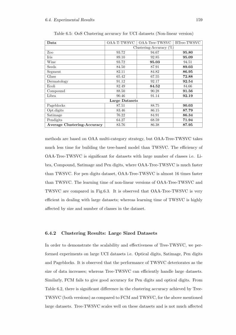
6.4. Experimental Results 159
Table 6.5: OoS Clustering accuracy for UCI datasets (Non-linear version)
Data OAA-T-TWSVC OAA-Tree-TWSVC BTree-TWSVC
Clustering-Accuracy (%)
Zoo 93.72 94.67 95.80
Iris 89.10 92.85 95.09
Wine 93.72 95.03 94.51
Seeds 84.50 87.91 89.03
Segment 82.11 84.82 86.95
Glass 65.42 67.55 72.88
Dermatology 91.12 92.17 92.54
Ecoli 82.49 84.52 84.66
Compound 88.50 90.28 91.56
Libra 90.46 91.14 92.19
Large Datasets
Pageblocks 87.51 88.75 90.03
Opt.digits 83.46 86.15 87.79
Satimage 76.22 84.91 86.34
Pendigits 64.27 68.59 71.94
Average Clustering-Accuracy 83.76 86.38 87.95
methods are based on OAA multi-category strategy, but OAA-Tree-TWSVC takes
much less time for building the tree-based model than TWSVC. The efficiency of
OAA-Tree-TWSVC is significant for datasets with large number of classes i.e. Li-
bra, Compound, Satimage and Pen digits, where OAA-Tree-TWSVC is much faster
than TWSVC. For pen digits dataset, OAA-Tree-TWSVC is almost 16 times faster
than TWSVC. The learning time of non-linear versions of OAA-Tree-TWSVC and
TWSVC are compared in Fig.6.3. It is observed that OAA-Tree-TWSVC is very
efficient in dealing with large datasets; whereas learning time of TWSVC is highly
affected by size and number of classes in the dataset.
6.4.2 Clustering Results: Large Sized Datasets
In order to demonstrate the scalability and effectiveness of Tree-TWSVC, we per-
formed experiments on large UCI datasets i.e. Optical digits, Satimage, Pen digits
and Pageblocks. It is observed that the performance of TWSVC deteriorates as the
size of data increases; whereas Tree-TWSVC can efficiently handle large datasets.
Similarly, FCM fails to give good accuracy for Pen digits and optical digits. From
Table 6.2, there is significant difference in the clustering accuracy achieved by Tree-
TWSVC (both versions) as compared to FCM and TWSVC, for the above mentioned
large datasets. Tree-TWSVC scales well on these datasets and is not much affected

160
Figure 6.2: Learning time (Linear)
Figure 6.3: Learning time (Non-linear)
by the number of classes.
6.5 Application: Image Segmentation
To evaluate the performance of Tree-TWSVC on large datasets, we present its ap-
plication on image segmentation which is a clustering problem. The image is par-
titioned into non-overlapping regions that share certain homogeneous features. For
the experiments, we have taken color images from Berkeley image segmentation
dataset (BSD) [57]. We use a dynamic method to determine the number of regions
for each image. The histogram for image is generated and the prominent peaks are
identified. The number of prominent peaks determine the number of regions (L)

6.6. Conclusions 161
in the image. The color image is then partitioned using minimum variance color
quantization with L levels. For the experiments, we have taken a combination of
color and texture features. The image features used for this work are Gabor texture
features [56] and RGB color value of the pixel. Gabor features are extracted with
4-orientation (0, 45, 90, 135) and 3-scale (0.5, 1.0, 2.0) sub-bands and the maximum
of the 12 coefficients determine the orientation at a given pixel location.
The segmentation model is built using OoS approach with BTree-TWSVC and
1% pixels are randomly selected from the image for learning. Rest of the image pixels
are used for testing the model. The images are segmented using BTree-TWSVC
and the results are compared with linear TWSVC and Multi-class Semi-supervised
Kernel Spectral Clustering (MSS-KSC) [95] segmentation methods, as shown in
Fig.6.4. MSS-KSC uses few labeled pixels to build the clustering model with Kernel
Spectral Clustering approach. It is observed that the segmentation results of BTree-
TWSVC are visually more accurate than other algorithms. For TWSVC, the image
is over-segmented, which results in formation of multiple smaller regions within
one large region. For BSD images, the ground truth segmentations are known and
the images segmented by BTree-TWSVC and TWSVC are compared with ground
truth. To statistically evaluate the segmentation algorithms, two evaluation criteria
are used: F-measure (FM) and error rate (ER). These measures are calculated with
respect to ground-truth boundaries and results are presented in Fig.6.4 and Table
6.6. BTree-TWSVC achieves better F-measure and error rate values than TWSVC
and MSS-KSC.
6.6 Conclusions
In this chapter, we present Tree-based Localized Fuzzy Twin Support Vector Clus-
tering (Tree-TWSVC) which is an iterative algorithm and extends the novel classi-
fier, Localized Fuzzy Twin Support Vector Machine (LF-TWSVM), in unsupervised
framework. Since, a patterns can not be associated with a unique cluster, our algo-
rithm determines fuzzy membership values for training patterns. LF-TWSVM is a
binary classifier that generates the non-parallel hyperplanes by solving system of lin-
ear equations. Tree-TWSVC develops a tree-based clustering model which consists

162
Figure 6.4: Segmentation results on BSD images (a.) Original image (b.) MSS-KSC(c.) TWSVC (d.) BTree-TWSVC
of several LF-TWSVM classifiers. In this chapter, we present two implementations
of Tree-TWSVC, namely Binary Tree-TWSVC and One-Against-All Tree-TWSVC.
Our clustering algorithm outperforms the other TWSVM-based clustering meth-
ods like TWSVC and F-LS-TWSVC, which are based on classical One-Against-All
multi-category approach and use Taylor’s series for approximating the constraints
of the optimization problem. Experimental results have proved that Tree-TWSVC
has superior clustering accuracy and efficient learning time for UCI datasets as com-
pared to FCM, TWSVC and F-LS-TWSVC. Our clustering algorithm is extended
for image segmentation problems also.

6.6. Conclusions 163
Table 6.6: Segmentation result for BSD color images
Image L F-measure Error rate
MSS-KSC TWSVC BTree-TWSVC MSS-KSC TWSVC BTree-TWSVC
385039 5 0.49 0.52 0.69 0.0726 0.0818 0.04998049 4 0.71 0.63 0.78 0.0784 0.0800 0.0676100007 3 0.57 0.57 0.66 0.0774 0.0798 0.0463295087 5 0.62 0.69 0.76 0.0910 0.0844 0.0527372019 4 0.49 0.47 0.54 0.0624 0.0755 0.0420388067 5 0.62 0.65 0.76 0.0980 0.1185 0.088755067 3 0.58 0.55 0.61 0.0214 0.0234 0.0201113044 3 0.71 0.63 0.73 0.0348 0.0400 0.0312118035 3 0.72 0.69 0.74 0.0513 0.0473 0.0431124084 3 0.54 0.48 0.69 0.0637 0.0818 0.0577161062 4 0.62 0.58 0.74 0.0343 0.0639 0.0168198023 4 0.57 0.58 0.78 0.0235 0.0363 0.0228388016 3 0.46 0.41 0.62 0.0806 0.1369 0.049051084 4 0.66 0.64 0.68 0.0695 0.0743 0.0613196027 4 0.63 0.45 0.67 0.0294 0.0359 0.0159

164

Chapter 7
Concluding Remarks
In this thesis, we have developed novel supervised and unsupervised learning algo-
rithms to perform the task of classification, clustering etc. To show the practical
application of our work, we have extended these machine learning techniques to
perform image processing tasks. Our work is motivated by nonparallel hyperplanes
classifier Twin Support Vector Machine (TWSVM). The objective is to develop
time-efficient algorithms which have better or comparable classification accuracy as
TWSVM-based algorithms.
With the emergence of new database technologies, an enormous amount of data
can be collected at very low cost. The decision ‘Whether data is apparent or not?’ is
deferred and everything is stored. This leads to a massive corpus for which machine
learning algorithms are required. The aim of our work is to develop algorithms
which can process huge amount of data in lesser time than existing algorithms. In
this chapter, we conclude our work along with discussion of advantages, pitfalls to
be avoided and future directions for extending this work.
7.1 Advantages of our Work
This thesis introduced time-efficient TWSVM-based classifiers which can effectively
handle large datasets. After analysis of TWSVM, it is observed that there is a scope
of improvement in terms of learning time and generalization ability. Since TWSVM
solves a pair of quadratic programming problems (QPPs) which also involves finding
inverse of a matrix, its learning time can be improved if the optimization problems
are formulated in a different manner. Working on this idea, we presented Improve-

166
ments of ν-Twin Support Vector Machine (Iν-TWSVM) which avoids solving QPPs
and instead solves unconstrained minimization problems (UMPs). It requires lesser
time to solve a UMP as it leads to solving a system of linear equations; whereas solv-
ing a QPP is more expensive. Iν-TWSVM considers ρ-distance separability between
patterns of one class and hyperplane of other class. Angle-based Twin Support Vector
Machine (ATWSVM) is another classifier which is developed on similar lines and
avoids solving QPPs. It is based on the concept of maximizing the angle between
two nonparallel hyperplanes.
In another binary classifier i.e. Angle-based Twin Parametric-margin Support
Vector Machine (ATP-SVM), only one optimization problem is formulated which
simultaneously determines both the nonparallel hyperplanes. The problem is for-
mulated so that it avoids solving inverse of matrices in the dual problem. The
learning time of this classifier is further improved by considering only representative
patterns while learning. These patterns are selected so that they can represent the
entire training set and therefore achieve good classification results. Since ATP-SVM
generates parametric-margin hyperplanes, it can efficiently handle heteroscedastic
noise.
Our work also includes a ternary tree based multi-category classification algo-
rithm, termed as Reduced Tree for Ternary Support Vector Machine (RT-TerSVM).
This algorithm uses a novel 3-class classifier, Ternary Support Vector Machine. This
work also includes development of algorithms which could extend existing binary
classifiers so as to handle multi-category data. These approaches are Ternary Deci-
sion Structure (TDS) and Binary Tree (BT) for extension of binary classifiers like
TWSVM, Generalized Eigenvalue Proximal SVM (GEPSVM) etc., to multi-category
scenario. All these algorithms are more efficient than classical multi-category algo-
rithms like One-Against-All, in terms of learning time and classification accuracy.
The success of plane-based classifiers motivated us to develop clustering algo-
rithms that use these classifiers in an iterative manner. Hence, we developed a
clustering algorithm based on TWSVM, termed as Tree-based Localized Fuzzy Twin
Support Vector Clustering (Tree-TWSVC). Tree-TWSVC builds the cluster model as
a Binary Tree of novel TWSVM-based classifier, termed as Localized Fuzzy TWSVM
(LF-TWSVM). Tree-TWSVC has efficient learning time, achieved due to tree struc-

7.2. Utility and Comparative Analysis of Algorithms 167
ture and the formulation that leads to solving a series of system of linear equations.
All the above mentioned algorithms have been successfully applied to perform
image processing tasks like image classification, content-based image retrieval and
segmentation.
7.2 Utility and Comparative Analysis of Algorithms
1. Iν-TWSVM improves the time complexity of TWSVM-based classifiers, by
replacing QPPs with UMPs and solves system of linear equations. Hence,
it can be used effectively to handle large datasets. The formulation of Iν-
TWSVM is attractive for handling unbalanced datasets. Another contribution
of this work is that Iν-TWSVM uses class representatives instead of considering
all the data patterns.
2. The concept of class representative is further improved in ATP-SVM, where a
subset of class patterns is created in a way that it represents the entire class.
These representative points capture the geometry of the class. Therefore, ATP-
SVM is more robust classifier than Iν-TWSVM. Also, ATP-SVM generates
both the hyperplanes simultaneously by solving one optimization problem and
is an effective classifier to handle noisy data. So, ATP-SVM does not require
parallel processing to generate hyperplanes, which is otherwise required by
classifiers, if both the hyperplanes are to be generated at the same time. Since
the dual problem of ATP-SVM does not require inverse of matrix, it solves an
efficient optimization problem.
3. ATWSVM presents a generic approach to transform any TWSVM-based clas-
sifier so that its time complexity can be improved without much affecting the
accuracy. It can efficiently handle large datasets. Its time-complexity is better
than that of ATP-SVM, whereas ATP-SVM is more robust than ATWSVM.
4. TerSVM is a ternary classifier and if required, can be used as binary classifier
also. TerSVM formulates all three problems as UMPs and can therefore handle
large-sized datasets. RT-TerSVM extends TerSVM to manage large number of
classes. TerSVM does not require dual formulation as required by ATP-SVM

168
and solves systems of linear equations to get the solution.
5. TDS is a generic multi-category approach which can be used with any TWSVM-
based classifier. Its time-complexity is better than that of RT-TerSVM.
6. Tree-TWSVC is an unsupervised algorithm developed for this work. It is used
to cluster data when labels are not available. Since patterns can not be crisply
associated with one cluster, Tree-TWSVC uses fuzzy memberships to initially
associate patterns with clusters.
7.3 Pitfalls to be Avoided
As discussed in the previous section, our work involves development of new classifi-
cation and clustering algorithms which are on the lines of TWSVM and its variants.
The success of machine learning projects depends on the quality of underlying classi-
fication and clustering algorithms. It is very important that these algorithms should
be carefully designed and implemented; otherwise the comparative study of these
algorithms can result in statistically wrong conclusions. The following section dis-
cusses the common pitfalls and the ways to avoid them.
Wrong selection of datasets
To authenticate the efficacy of our algorithm, we use empirical validation. The
machine learning community has developed and maintained some benchmark data
repositories like UC Irvine (UCI) Machine Learning Repository [52], which currently
has 378 datasets. These datasets are available to perform numerical experiments to
validate different algorithms. The datasets should be carefully chosen for performing
experiments and should not be restricted to only four or five. There should be a right
mix of datasets, varying from small-sized (i.e. number of instances) to large-sized;
those with few attributes to large number of attributes. The synthetic datasets
should be cautiously picked or created, which can highlight the contribution of our
work.
There are few datasets in UCI repository with missing values like Dermatology,
Hepatitis etc. To use such datasets, some value must be assigned for the missing

7.3. Pitfalls to be Avoided 169
data. Do not set ‘0’ for numerical attributes. A better option is to fill the miss-
ing values, in numerical attributes, with the mean of the corresponding feature’s
remaining values and missing logical values could be replaced with the value that
appears maximum number of times for that attribute.
Incomplete comparative study
The proposed algorithms are compared with existing methods to prove the efficacy
of our work. At first glance, these studies may appear to be quite easy to do,
but in reality it requires considerable skill and a thorough knowledge of underlying
mathematics, to be successful at both improving known algorithms and designing the
experiments. The empirical validation is necessary but not sufficient to establish the
efficacy of our algorithm. Some statistical tests should also be performed to compare
multiple algorithms. In our work, we have compared algorithms using Friedman test
[54] and Holm-Bonferroni test [55].
Random tuning of parameters
Researchers tune the parameters repeatedly, so that the algorithms can perform
optimally on the chosen datasets. While experimenting with the algorithms, a great
deal of time is spent in determining the optimal parameter values. During parameter
tuning, every change should be considered as a separate experiment. Instead of
randomly selecting the parameters, grid search method [50] should be used.
Conventional validation
Conventional validation which partitions the data set into two sets of ratio 70 : 30
for training-test data, is not appropriate for conducting experiments. For a model
with one or more user-defined parameters and a fixed training set, the tuning process
optimizes the model parameters so that the model fits the training data as accurately
as possible. If we then take an unseen sample of test data, it is observed that the
model does not fit the test data as well as it fits the training data. This is called
over-fitting and it generally happens when the size of the training dataset is small, or
when the number of parameters in the model is large. To generate unbiased results,
the training and test set should be created using cross validation [49]. It segments

170
the dataset such that in each fold a new segment is taken as training set. When
the parameters get the optimal settings, accuracy can be measured on the test data.
This gives an opportunity to the researcher to test the algorithm with unseen data.
The final accuracy should be the mean accuracy over all the folds.
7.4 The Road-map Ahead
The following future trends of our research are identified, which can extend our work
in new directions.
• In our thesis, supervised and unsupervised machine learning algorithms have
been developed. There are various real time applications like video surveil-
lance, medical imaging etc. where the data is available in large amounts, but
it is expensive to obtain their labels. For such applications, semi-supervised
classification algorithms can be developed. Our binary classifiers can be used
in semi-supervised framework as Qi et al. proposed Laplacian Twin Support
Vector Machine for semi-supervised classification [96].
• Working in the spirit of Khemchandani et al. [97], future line of work could be
to discuss the kernel selection problem of our binary classifiers like Iν-TWSVM,
ATP-SVM etc. over the convex set of finitely many basic kernels, which can
be formulated as an iterative alternating optimization problem.
• Most of the SVM and TWSVM based classification algorithms assume that
the entire training data could fit into main memory. With the growth of
businesses, the amount of data exceeds the memory limit, which is available
to the learning systems. Hence, there is a need to identify scalable algorithms
for classification. These algorithms could be implemented in the framework of
incremental learning.
• When the optimization problem is independent of inverse of matrix, it can
be solved by efficient Sequential Minimal Optimization (SMO) [62] technique.
Since, the dual of ATP-SVM does not involve inverse of matrices, it could
be implemented using SMO. Another work could be to explore angle-based
methodology like ATP-SVM and ATWSVM, for regression problems.

7.4. The Road-map Ahead 171
• In order to apply our algorithms to large-scale data mining processes, there
is a need to make them even more computationally efficient. The potential
direction in this regard is the parallelization of training phase especially for
multi-category classification algorithms.
• Future work could be to develop a sparse algorithm version for our classifiers
like Iν-TWSVM, ATP-SVM, TerSVM etc.
• We could also explore the option of combining two or more machine learning
algorithms to get a new, efficient algorithm.

172

References
[1] C. Cortes, V. Vapnik, Support-vector networks, Machine Learning 20 (3)
(1995) 273–297.
[2] C. J. Burges, A tutorial on support vector machines for pattern recognition,
Data Mining and Knowledge Discovery 2 (2) (1998) 121–167.
[3] V. N. Vapnik, An overview of statistical learning theory, IEEE Transactions
on Neural Networks, 10 (5) (1999) 988–999.
[4] V. Vapnik, The nature of statistical learning theory, Springer Science & Busi-
ness Media, 2000.
[5] O. L. Mangasarian, D. R. Musicant, Lagrangian support vector machines, The
Journal of Machine Learning Research 1 (2001) 161–177.
[6] Y.-J. Lee, O. L. Mangasarian, Ssvm: A smooth support vector machine for
classification, Computational Optimization and Applications 20 (1) (2001) 5–
22.
[7] J. A. Suykens, J. Vandewalle, Least squares support vector machine classifiers,
Neural Processing Letters 9 (3) (1999) 293–300.
[8] O. L. Mangasarian, E. W. Wild, Proximal support vector machine classifiers,
in: Proceedings KDD-2001: Knowledge Discovery and Data Mining, Citeseer,
2001.
[9] O. L. Mangasarian, E. W. Wild, Multisurface proximal support vector ma-
chine classification via generalized eigenvalues, IEEE Transactions on Pattern
Analysis and Machine Intelligence, 28 (1) (2006) 69–74.

174
[10] Jayadeva, R. Khemchandani, S. Chandra, Twin support vector machines for
pattern classification, IEEE Transactions on Pattern Analysis and Machine
Intelligence 29 (5) (2007) 905–910.
[11] R. Khemchandani, Mathematical programming applications in machine learn-
ing, Ph.D. thesis, Indian Institute of Technology Delhi New Delhi-110016,
India (2008).
[12] Jayadeva, R. Khemchandani, S. Chandra, Twin Support Vector Machines:
Models, Extensions and Applications, Vol. 659, Springer, 2016.
[13] O. L. Mangasarian, Nonlinear programming, Vol. 10, SIAM, 1993.
[14] M. A. Kumar, M. Gopal, Least squares twin support vector machines for
pattern classification, Expert Systems with Applications 36 (4) (2009) 7535–
7543.
[15] Y.-H. Shao, C.-H. Zhang, X.-B. Wang, N.-Y. Deng, Improvements on twin sup-
port vector machines, IEEE Transactions on Neural Networks, 22 (6) (2011)
962–968.
[16] X. Peng, Tpmsvm: a novel twin parametric-margin support vector machine
for pattern recognition, Pattern Recognition 44 (10) (2011) 2678–2692.
[17] P.-Y. Hao, New support vector algorithms with parametric insensitive/margin
model, Neural Networks 23 (1) (2010) 60–73.
[18] X. Peng, A ν-twin support vector machine (ν-tsvm) classifier and its geometric
algorithms, Information Sciences 180 (20) (2010) 3863–3875.
[19] Y.-J. Tian, X.-C. Ju, Nonparallel support vector machine based on one opti-
mization problem for pattern recognition, Journal of the Operations Research
Society of China 3 (4) (2015) 499–519.
[20] T. Hastie, R. Tibshirani, J. Friedman, Unsupervised learning, Springer, 2009.
[21] A. K. Jain, R. C. Dubes, Algorithms for clustering data, Prentice-Hall, Inc.,
1988.

7.4. The Road-map Ahead 175
[22] A. Y. Ng, M. I. Jordan, Y. Weiss, et al., On spectral clustering: Analysis and
an algorithm, Advances in Neural Information Processing Systems 2 (2002)
849–856.
[23] J. Shi, J. Malik, Normalized cuts and image segmentation, IEEE Transactions
on Pattern Analysis and Machine Intelligence, 22 (8) (2000) 888–905.
[24] W. Wu, H. Xiong, S. Shekhar, Clustering and information retrieval, Vol. 11,
Springer Science & Business Media, 2013.
[25] A. K. Jain, Data clustering: 50 years beyond k-means, Pattern Recognition
Letters 31 (8) (2010) 651–666.
[26] X. Wang, Y. Wang, L. Wang, Improving fuzzy c-means clustering based on
feature-weight learning, Pattern Recognition Letters 25 (10) (2004) 1123–1132.
[27] L. Xu, J. Neufeld, B. Larson, D. Schuurmans, Maximum margin clustering,
Advances in Neural Information Processing Systems 17 (2004) 1537–1544.
[28] Z. Wang, Y.-H. Shao, L. Bai, N.-Y. Deng, Twin support vector machine for
clustering, Neural Networks and Learning Systems, IEEE Transactions on
26 (10) (2015) 2583–2588.
[29] K. Zhang, I. W. Tsang, J. T. Kwok, Maximum margin clustering made prac-
tical, IEEE Transactions on Neural Networks, 20 (4) (2009) 583–596.
[30] A. L. Yuille, A. Rangarajan, The concave-convex procedure, Neural Compu-
tation 15 (4) (2003) 915–936.
[31] A. J. Smola, B. Scholkopf, Learning with kernels, Citeseer, 1998.
[32] C.-W. Hsu, C.-J. Lin, A comparison of methods for multiclass support vector
machines, IEEE Transactions on Neural Networks, 13 (2) (2002) 415–425.
[33] J. C. Platt, N. Cristianini, J. Shawe-Taylor, Large margin dags for multiclass
classification., in: nips, Vol. 12, 1999, pp. 547–553.
[34] Jayadeva, R. Khemchandani, S. Chandra, Fuzzy linear proximal support vec-
tor machines for multi-category data classification, Neurocomputing 67 (2005)
426–435.

176
[35] H. Lei, V. Govindaraju, Half-against-half multi-class support vector machines,
in: Multiple Classifier Systems, Springer, 2005, pp. 156–164.
[36] Y.-H. Shao, W.-J. Chen, W.-B. Huang, Z.-M. Yang, N.-Y. Deng, The best sep-
arating decision tree twin support vector machine for multi-class classification,
Procedia Computer Science 17 (2013) 1032–1038.
[37] J. Xie, K. Hone, W. Xie, X. Gao, Y. Shi, X. Liu, Extending twin support
vector machine classifier for multi-category classification problems, Intelligent
Data Analysis 17 (4) (2013) 649–664.
[38] C. Angulo, X. Parra, A. Catala, K-svcr. a support vector machine for multi-
class classification, Neurocomputing 55 (1) (2003) 57–77.
[39] Y. Xu, R. Guo, L. Wang, A twin multi-class classification support vector
machine, Cognitive computation 5 (4) (2013) 580–588.
[40] B. Scholkopf, P. L. Bartlett, A. J. Smola, R. Williamson, Shrinking the tube:
a new support vector regression algorithm, Advances in Neural Information
Processing Systems (1999) 330–336.
[41] B. Scholkopf, A. J. Smola, R. C. Williamson, P. L. Bartlett, New support
vector algorithms, Neural Computation 12 (5) (2000) 1207–1245.
[42] M. R. Guarracino, C. Cifarelli, O. Seref, P. M. Pardalos, A classification
method based on generalized eigenvalue problems, Optimisation Methods and
Software 22 (1) (2007) 73–81.
[43] Y.-H. Shao, N.-Y. Deng, W.-J. Chen, Z. Wang, Improved generalized eigen-
value proximal support vector machine, Signal Processing Letters, IEEE 20 (3)
(2013) 213–216.
[44] S. R. Gunn, et al., Support vector machines for classification and regression,
ISIS technical report 14.
[45] J. Nocedal, S. Wright, Numerical optimization, Springer Science & Business
Media, 2006.

7.4. The Road-map Ahead 177
[46] S. Chandra, Jayadeva, A. Mehra, Numerical optimization with Applications,
Alpha Science International, 2009.
[47] J. A. Hartigan, M. A. Wong, Algorithm as 136: A k-means clustering algo-
rithm, Applied Statistics (1979) 100–108.
[48] V. J. Hodge, J. Austin, A survey of outlier detection methodologies, Artificial
Intelligence Review 22 (2) (2004) 85–126.
[49] R. O. Duda, P. E. Hart, D. G. Stork, Pattern classification, John Wiley &
Sons, 2012.
[50] C. J. Lin, C.-W. Hsu, C.-C. Chang, A practical guide to support
vector classification, 2003, National Taiwan U., www. csie. ntu. edu.
tw/cjlin/papers/guide/guide. pdf.
[51] M. Belkin, P. Niyogi, V. Sindhwani, Manifold regularization: A geometric
framework for learning from labeled and unlabeled examples, The Journal of
Machine Learning Research 7 (2006) 2399–2434.
[52] C. Blake, C. J. Merz, Uci repository of machine learning databases.
URL http://www.ics.uci.edu/~mlearn/MLRepository.html,1998.
[53] D. Musicant, Ndc: normally distributed clustered datasets, Computer Sciences
Department, University of Wisconsin, Madison 1998.
URL <http://www.cs.wisc.edu/~musicant/data/ndc>
[54] J. Demsar, Statistical comparisons of classifiers over multiple data sets, The
Journal of Machine Learning Research 7 (2006) 1–30.
[55] S. Holm, A simple sequentially rejective multiple test procedure, Scandinavian
journal of statistics (1979) 65–70.
[56] J. F. Khan, R. R. Adhami, S. M. Bhuiyan, A customized gabor filter for
unsupervised color image segmentation, Image and Vision Computing 27 (4)
(2009) 489–501.

178
[57] P. Arbelaez, C. Fowlkes, D. Martin, The berkeley segmenta-
tion dataset and benchmark, see http://www. eecs. berkeley.
edu/Research/Projects/CS/vision/bsds.
[58] Y.-H. Shao, W.-J. Chen, N.-Y. Deng, Nonparallel hyperplane support vector
machine for binary classification problems, Information Sciences 263 (2014)
22–35.
[59] R. Khemchandani, P. Saigal, Color image classification and retrieval through
ternary decision structure based multi-category twsvm, Neurocomputing 165
(2015) 444–455.
[60] R. Khemchandani, P. Saigal, S. Chandra, Improvements on ν-twin support
vector machine, Neural Networks 79 (2016) 97–107.
[61] Y. Tian, X. Ju, Z. Qi, Y. Shi, Improved twin support vector machine, Science
China Mathematics 57 (2) (2014) 417–432.
[62] X. Peng, Tsvr: an efficient twin support vector machine for regression, Neural
Networks 23 (3) (2010) 365–372.
[63] B. D. Ripley, Pattern recognition and neural networks, Cambridge university
press, 2007.
[64] Y.-J. Lee, O. L. Mangasarian, Rsvm: Reduced support vector machines., in:
SDM, Vol. 1, 2001, pp. 325–361.
[65] B. S. Manjunath, W.-Y. Ma, Texture features for browsing and retrieval of
image data, Pattern Analysis and Machine Intelligence, IEEE Transactions on
18 (8) (1996) 837–842.
[66] W. Tao, H. Jin, Y. Zhang, Color image segmentation based on mean shift and
normalized cuts, IEEE Transactions on Systems, Man, and Cybernetics, Part
B (Cybernetics) 37 (5) (2007) 1382–1389.
[67] P. Simard, Y. LeCun, J. S. Denker, Efficient pattern recognition using a new
transformation distance, Advances in neural information processing systems
(1993) 50–50.

7.4. The Road-map Ahead 179
[68] P. Y. Simard, Y. A. LeCun, J. S. Denker, B. Victorri, Transformation in-
variance in pattern recognitiontangent distance and tangent propagation, in:
Neural networks: tricks of the trade, Springer, 1998, pp. 239–274.
[69] D. Keysers, T. Deselaers, C. Gollan, H. Ney, Deformation models for image
recognition, IEEE Transactions on Pattern Analysis and Machine Intelligence
29 (8).
[70] Y. Liu, D. Zhang, G. Lu, W.-Y. Ma, A survey of content-based image retrieval
with high-level semantics, Pattern recognition 40 (1) (2007) 262–282.
[71] A. N. Tikhonov, V. I. Arsenin, Solutions of ill-posed problems, Vh Winston,
1977.
[72] B. N. Parlett, The symmetric eigenvalue problem, Vol. 7, SIAM, 1980.
[73] B. S. Manjunath, J.-R. Ohm, V. V. Vasudevan, A. Yamada, Color and texture
descriptors, IEEE Transactions on circuits and systems for video technology
11 (6) (2001) 703–715.
[74] M. Subrahmanyam, Q. J. Wu, R. Maheshwari, R. Balasubramanian, Modified
color motif co-occurrence matrix for image indexing and retrieval, Computers
& Electrical Engineering 39 (3) (2013) 762–774.
[75] M. E. ElAlami, A novel image retrieval model based on the most relevant
features, Knowledge-Based Systems 24 (1) (2011) 23–32.
[76] S. Murala, Q. J. Wu, Expert content-based image retrieval system using robust
local patterns, Journal of Visual Communication and Image Representation
25 (6) (2014) 1324–1334.
[77] E. Walia, A. Pal, D. Pandian, D. Lohani, Variant of completed robust lbp
for two-level probabilistic content based image retrieval, Proceedings of Com-
puter and Advanced Technology in Education http://dx. doi. org/10.2316/P
3 (2014) 2014.

180
[78] A. H. Reddy, N. S. Chandra, Local oppugnant color space extrema patterns for
content based natural and texture image retrieval, AEU-International Journal
of Electronics and Communications 69 (1) (2015) 290–298.
[79] S. Murala, R. Maheshwari, R. Balasubramanian, Directional local extrema
patterns: a new descriptor for content based image retrieval, International
journal of multimedia information retrieval 1 (3) (2012) 191–203.
[80] K. P. Jasmine, P. R. Kumar, Color and local maximum edge patterns his-
togram for content based image retrieval, International Journal of Intelligent
Systems and Applications 6 (11) (2014) 66.
[81] T. Ojala, M. Pietikainen, T. Maenpaa, Multiresolution gray-scale and rotation
invariant texture classification with local binary patterns, IEEE Transactions
on pattern analysis and machine intelligence 24 (7) (2002) 971–987.
[82] P. S. Bradley, O. L. Mangasarian, k-plane clustering, Journal of Global Opti-
mization 16 (1) (2000) 23–32.
[83] Y.-H. Shao, L. Bai, Z. Wang, X.-Y. Hua, N.-Y. Deng, Proximal plane clustering
via eigenvalues, Procedia Computer Science 17 (2013) 41–47.
[84] H. Valizadegan, R. Jin, Generalized maximum margin clustering and unsuper-
vised kernel learning, in: Advances in Neural Information Processing Systems,
2006, pp. 1417–1424.
[85] S. Boyd, L. Vandenberghe, Convex optimization, Cambridge university press,
2004.
[86] M. S. Lobo, L. Vandenberghe, S. Boyd, H. Lebret, Applications of second-
order cone programming, Linear Algebra and its Applications 284 (1) (1998)
193–228.
[87] R. Khemchandani, A. Pal, S. Chandra, Fuzzy least squares twin support vector
clustering, Neural Computing and Applications (2016) 1–11.
[88] Z.-M. Yang, Y.-R. Guo, C.-N. Li, Y.-H. Shao, Local k-proximal plane cluster-
ing, Neural Computing and Applications 26 (1) (2015) 199–211.

7.4. The Road-map Ahead 181
[89] D. T. Larose, k-nearest neighbor algorithm, Discovering Knowledge in Data:
An Introduction to Data Mining (2005) 90–106.
[90] D. P. Huttenlocher, G. A. Klanderman, W. J. Rucklidge, Comparing images
using the hausdorff distance, IEEE Transactions on Pattern Analysis and Ma-
chine Intelligence, 15 (9) (1993) 850–863.
[91] T. H. Cormen, Introduction to algorithms, MIT press, 2009.
[92] P.-N. Tan, M. Steinbach, V. Kumar, Introduction to data mining addison-
wesley (2005).
[93] C. Alzate, J. A. Suykens, Multiway spectral clustering with out-of-sample ex-
tensions through weighted kernel pca, IEEE Transactions on Pattern Analysis
and Machine Intelligence, 32 (2) (2010) 335–347.
[94] C. Alzate, J. A. K. Suykens, Out-of-sample eigenvectors in kernel spectral
clustering, in: The 2011 International Joint Conference on Neural Networks
(IJCNN),, IEEE, 2011, pp. 2349–2356.
[95] S. Mehrkanoon, C. Alzate, R. Mall, R. Langone, J. Suykens, et al., Multiclass
semisupervised learning based upon kernel spectral clustering, IEEE Transac-
tions on Neural Networks and Learning Systems, 26 (4) (2015) 720–733.
[96] Z. Qi, Y. Tian, Y. Shi, Laplacian twin support vector machine for semi-
supervised classification, Neural Networks 35 (2012) 46–53.
[97] R. Khemchandani, Jayadeva, S. Chandra, Optimal kernel selection in twin
support vector machines, Optimization Letters 3 (1) (2009) 77–88.
[98] R. J. Simes, An improved bonferroni procedure for multiple tests of signifi-
cance, Biometrika 73 (3) (1986) 751–754.
[99] Y.-H. Shao, N.-Y. Deng, Z.-M. Yang, Least squares recursive projection twin
support vector machine for classification, Pattern Recognition 45 (6) (2012)
2299–2307.
[100] N. L. Johnson, S. Kotz, N. Balakrishnan, Lognormal distributions, Continuous
Univariate Distributions, 1, 1994.

182
[101] Z. Guo, L. Zhang, D. Zhang, A completed modeling of local binary pattern
operator for texture classification, IEEE Transactions on Image Processing
19 (6) (2010) 1657–1663.
[102] Y. Zhao, W. Jia, R.-X. Hu, H. Min, Completed robust local binary pattern
for texture classification, Neurocomputing 106 (2013) 68–76.
[103] A. Amanatiadis, V. Kaburlasos, A. Gasteratos, S. Papadakis, Evaluation of
shape descriptors for shape-based image retrieval, IET Image Processing 5 (5)
(2011) 493–499.
[104] J. Z. Wang, J. Li, G. Wiederhold, Simplicity: Semantics-sensitive integrated
matching for picture libraries, Pattern Analysis and Machine Intelligence,
IEEE Transactions on 23 (9) (2001) 947–963.
[105] Corel 10000 image database.
URL wang.ist.psu.edu/docs/related
[106] Mit vistex database of textures, media laboratory,.
URL http://vismod.media.mit.edu/vismod/imagery/VisionTexture/
[107] Oliva and torralba scene dataset,.
URL http://cvcl.mit.edu/database.htm

Appendices
183


Appendix A
Evaluation Measures
1. Accuracy:
‘Accuracy’ of a classification algorithm is defined as follows
Accuracy =TP + TN
TP + FP + TN + FN. (A.1)
Here TP, TN, FP, and FN are the number of true positive, true negative, false
positive and false negative respectively.
2. Friedman test:
The Friedman test [54] is a non-parametric test for comparing three or more
related samples and it makes no assumptions about the underlying distribu-
tion of the data. The data is set out in a table comprising of n1 rows and
n2 columns. It ranks the algorithms for each dataset separately, the best per-
forming algorithm getting the rank of 1, the second best rank 2 and so on. In
case of ties, average ranks are assigned. It then compares the average ranks of
algorithms, Rj = 1NΣir
ji where rji is the rank of the jth algorithm on the ith
dataset of N dataset.
3. p-value and Holm-Bonferroni test:
The p-value [54] is calculated by performing pairwise t-test. The null hypothe-
sis assumes that the data of two-sample t-test comes from independent random
samples with equal means and equal but unknown variances. The p-values are
tested for a significance level α = 0.05.
To analyze the performance of multiple algorithms, Holm-Bonferroni method

186
[98] is used. It compares the algorithms and tests their hypotheses. Let there
are N statistics T1, ..., TN with corresponding p-values P1, ..., PN for test hy-
pothesis H1, ...,HN . For a significance level α, Holm-Bonferroni test orders
the p-values from minimum to maximum as P(1), ..., P(N) with corresponding
null hypothesis H(1), ...,H(N). It rejects the null hypotheses H(1), ...,H(k−1)
and does not reject H(k), ...,H(N), if
P(k) >α
N + 1− k.
4. F-measure (FM) and error rate (ER):
To evaluate the segmentation algorithms statistically, F-measure is used which
is harmonic mean of precision and recall and is given by
FM =2× Precision×RecallPrecision+Recall
, (A.2)
and ER is given by
ER =FP + FN
Total number of patterns, (A.3)
where Precision and Recall are defined as
Precision =TP
TP + FP,
Recall =TP
TP + FN.
TP, FP, TN, FN are true-positive, false-positive, true-negative and false-
negative respectively. For color image segmentation problems, these measures
are calculated with respect to ground-truth boundaries of images.
5. Average Retrieval Rate:
The (P-R) ratio is measured using (A.4) and (A.5).
Precision =Number of relevant images retrieved
Number of retrieved images, (A.4)
Recall =Number of relevant images retrieved
Total number of relevant images. (A.5)

187
Average Retrieval Rate (ARR) [73] is a robust metric for comparison of image
retrieval methods. It can be computed using (A.6).
ARR =1
N
NQ∑q=1
RR(q) (A.6)
where NQ represents the number of queries that are used for the purpose of
verifying the descriptor in some dataset. RR(q) represents the retrieval rate of
a single query and RR(q) ≤ 1. In our experiments, each image in the database
is treated as the query image and average over the entire database gives the
performance of the retrieval method.
6. Clustering-Accuracy:
The metric Clustering-Accuracy [92] is used to measure the performance of
clustering methods. For finding the accuracy of clustering algorithm, a simi-
larity matrix S ∈ Rm×m is computed with the given data labels yi, yj ∈ 1 :
K, i = 1 : m, j = 1 : m, where
S(i, j) =
1, if yi = yj
0, otherwise.
Let St and Sp are the similarity matrices computed by the true cluster labels
and predicted labels respectively. The accuracy of clustering method is defined
as the Rand statistic [92] and is given as
Clustering −Accuracy =nzeros + nones −m
m2 −m× 100 (A.7)
where nzeros is the number of zeros at corresponding indices in both St and
Sp, and nones is the number of ones in both St and Sp.

188

Appendix B
Loss Function of TWSVM
TWSVM uses hinge loss function which is given by
Lh =
0, yifi ≥ 1
1− yifi, otherwise
For any SVM or TWSVM based clustering method, the clustering error or the hy-
perplanes change little after initial labeling or during subsequent iterations. This
arises due to hinge loss function, as shown in Fig.B.1a, where the classifier tries to
push yifi to the point beyond yifi = 1 (towards right) [29]. Here, solid line shows
loss with initial labels and dotted line shows loss after flipping of labels. As observed
from the empirical margin distribution of yifi, most of the patterns have margins
yifi 1. If the label of a pattern is changed, the loss will be very large and the
classifier is unwilling to flip the class labels. So, the procedure gets stuck in a lo-
cal optimum and adheres to the initial label estimates. To prevent the premature
convergence of the iterative procedure, the loss function is changed to square loss
and is given as Ls = (1 − yifi)2. This loss function is symmetric around yifi = 1,
as shown in Fig.B.1b and penalizes preliminary wrong predictions. Therefore, it
permits flipping of labels if needed and leads to a significant improvement in the
clustering performance.

190
(a) Hinge loss function (b) Square loss function
Figure B.1: Flipping of labels. a. Hinge loss function; b. Square loss function

Appendix C
UCI Datasets
The binary UCI datasets [52] used for numerical experiments in our work, are listed
below:
1. Australian Credit Approval Dataset (ACA) (690 × 14): This dataset has 690
instances with 14 attributes. The two classes contain 383 and 307 patterns,
related to credit card applications. It has a variety of attributes - continuous,
nominal and binary.
2. Breast Cancer Wisconsin Prognostic (WPBC) (698 × 34): For this dataset,
the problem is to predict accurately the presence or absence of a malignant
tumor, with 458 benign and 240 malignant patterns.
3. BUPA Liver Disorders Data Set (345 × 7): Each record represents the blood
test reports of a single male individual. The first five attributes are tests which
are sensitive to liver disorders arising from from excessive alcohol consumption.
The patterns are distributed as 200 and 145 in two classes.
4. Cleveland Heart Disease Dataset (Heart-C) (303 × 13): The original database
has 76 attributes, but most of the published experiments use a subset of 14
attributes. The problem is to predict the presence of heart disease in a patient
(“goal” values 1,2,3,4) or absence (value 0). The dataset contains 164 positive
and 139 negative instances.
5. Congressional Voting Records Dataset (Votes) (435 × 16): This dataset con-
sists of 1984 United Stated Congressional Voting Records with two classes-
Republican (267) or Democratic (168).

192
6. Connectionist Bench Sonar Dataset(208 × 60): The problem is to classify
sonar signals bounced off a metal cylinder and those bounced off a roughly
cylindrical rock. The are 111 patterns obtained by bouncing sonar signals off
a metal cylinder at various angles and 97 patterns obtained from rocks under
similar conditions. Each pattern has 60 numeric attributes.
7. Contraceptive Method Choice Dataset (CMC) (1473 × 9): This dataset is a
subset of the 1987 National Indonesia Contraceptive Prevalence Survey. The
patterns were married women who were either not pregnant or do not know
if they were at the time of interview. The problem is to predict the current
contraceptive method choice of a woman based on her demographic and socio-
economic characteristics. The two classes represent contraceptive users (844)
and non-users (629).
8. German Credit Dataset (1000 × 20): This numeric dataset contains credit
data and is produced by Strathclyde University. All the categorical attributes
have been coded as integers. The instances are labeled as “good” (700) and
“bad” (300).
9. Heart Statlog Dataset (Heart-S) (270 × 13): This dataset contains 13 real,
binary and nominal attributes, with 150 positive and 120 negative patterns.
10. Ionosphere Dataset (351 × 34): This dataset contains radar data, collected by
a system in Goose Bay, Labrador. It classifies free electrons in the ionosphere
as “Good” (225) when radar returns show evidence of some type of structure
in the ionosphere and “Bad” (126) otherwise.
11. Pima Indians Diabetes Dataset (768 × 8): This data is collected by National
Institute of Diabetes and Digestive and Kidney Diseases. All the patients
are females at least 21 years old of Pima Indian heritage. 500 instances are
negative while 268 are positive ones.
12. Thyroid Disease Dataset (215 × 5): This data is collected by Stefan Aeberhard
and has 150 and 65 negative and positive patterns respectively.
13. Two-norm Dataset (400 × 20): This is a dataset with two classes of 351 and

193
49 instances.
The UCI multi-category datasets [52] used for numerical experiments are:
1. Dermatology Dataset (366 × 34, 6 classes): This dataset is used to predict the
type of Eryhemato-Squamous Disease in dermatology. It has 34 attributes, 33
of which are linear valued and one is nominal.
2. Ecoli Dataset (336× 7, 8 classes): This dataset contains records for protein
localization sites and is created by Kenta Nakai.
3. Glass Identification Dataset (Glass) (214× 9, 6 classes): This data is generated
by USA Forensic Science Service. It has instances for six types of glasses
defined in terms of their oxide content. The study of glass was motivated by
criminology investigation, where the glass left behind at crime scene can be
used as evidence, if it is correctly identified.
4. Iris Dataset (150 × 4, 3 classes): This is a well known dataset often used to
test the efficacy of pattern recognition method, first used by Fisher in 1936.
The dataset has 3 classes of 50 instances each, where each class refers to a
type of iris plant. One class is linearly separable from the other 2; the latter
are NOT linearly separable from each other.
5. Libras (360 × 91, 15 classes): The dataset contains 15 classes of 24 instances
each. Each class references to a hand movement type in LIBRAS (Portuguese
name ’Lngua BRAsileira de Sinais’, oficial brazilian signal language).
6. Multiple Features Dataset (MF) (2,000 × 649, 10 classes): This dataset con-
sists of features of handwritten numerals (‘0’-‘9’) extracted from a collection
of Dutch utility maps. 200 patterns per class (for a total of 2,000 patterns)
have been digitized in binary images.
7. Optical Recognition of Handwritten Digits Dataset (Optical digits or OD)
(5,620 × 64, 10 classes): This data describes bitmaps of handwritten digits.
43 people contributed for data collection. 32 × 32 bitmaps are divided into
non-overlapping blocks of 4x4 and the number of on pixels are counted in each
block.

194
8. Page Blocks Classification Dataset (PB) (5,473 × 10, 5 classes): The problem
is to classify all the blocks of the page layout of a document that has been
detected by a segmentation process. It has 5473 patterns taken from 54 distinct
documents, where each instance concerns one block.
9. Satimage (6435 × 36, 7 classes): Multi-spectral values of pixels in 3x3 neigh-
borhoods in a satellite image, and the classification associated with the cen-
tral pixel in each neighborhood. The original Landsat data for this database
was generated from data purchased from NASA by the Australian Centre for
Remote Sensing, and used for research at The Centre for Remote Sensing,
University of New South Wales, Australia.
10. Seeds Dataset (210 × 7, 3 classes): This data contains records of geometrical
properties of kernels belonging to three different varieties of wheat. The pat-
tern instances are generated by soft X-ray technique and GRAINS package to
construct 7 real-valued attributes.
11. Statlog Image Segmentation Dataset (Segment) (210× 19, 7 classes): This
dataset is an image segmentation database where the instances are randomly
selected from a database of seven outdoor images. The images are hand-
segmented to create a classification for every pixel.
12. Wine Dataset(178× 13, 3 classes): This data is generated by chemical anal-
ysis of wines grown in the same region in Italy but raised by three different
cultivators. It has 13 attributes listing the quantity of constituents found in
each pattern of wine.
13. Zoo Dataset (101× 16, 7 classes): This database of animal types in a zoo,
contains boolean-valued attributes.

Appendix D
Synthetic Datasets
Dataset 1: Cross planes
The cross-planes data [8] consists of data points lying near two intersecting lines. It
can be considered as a perturbed generalization of exclusive-OR (XOR) classification
problem. Fig.D.1a illustrates the cross planes data with 200 training points. The
red ‘dots’ and blue ‘plus’ represent the data points of two classes.
(a) Cross planes data (b) Syn1 data
(c) Ripley’s data(d) Complex XOR data
Figure D.1: Synthetic Datasets

196
Dataset 2: Syn1 data
The dataset Syn1, as shown in Fig. D.1b, has patterns in R2, created with
+1 : x = [ρcosθ, ρsinθ], ρ ∼ U(0, 1), θ ∼ U(0, π/3),
−1 : x = [ρcosθ, ρsinθ], ρ ∼ U(0, 1), θ ∼ U(π/2, 5π/6), (D.1)
where U(a, b) denotes the uniform distribution in (a, b) and 100 data points are
randomly created for both the classes.
Dataset 3: Ripley’s data
The Ripleys dataset is an artificially-generated binary dataset [63] which includes
250 training points and 1000 test points, as shown in Fig.D.1c.
Dataset 4: Complex XOR
Mangasarian et al. [9] proposed nonparallel hyperplanes classifier GEPSVM and
established its efficacy using cross-planes data. This dataset is generated as data
points lying near two intersecting lines and is considered as perturbed generalization
of exclusive-OR (XOR) classification problem. We have performed experiments with
complex XOR dataset [99], which is generalization of XOR problem, with added
white Gaussian noise. Fig.D.1d shows the nonparallel planes obtained with linear
version of ATWSVM and TBSVM. The data consists of 120 patterns in R2 where
red ‘dots’ (80) and blue ‘stars’ (40) represent the data points of positive and negative
classes respectively.
Dataset 5: Two-moons
The two moons dataset [51], as shown in Fig.D.2 consists of 200 data points in R2,
belonging to two classes.
Dataset 6: NDC and Exp-NDC
NDC data is generated using David Musicants NDC Data Generator [53] and is
normally distributed. The NDC datasets are skewed by making use of log-normal

197
Figure D.2: Two moons dataset
distribution [100]. In probability theory, a continuous random variable whose log-
arithm is normally distributed, is said to possess log-normal distribution. Thus, if
the random variable X1 is log-normally distributed, then X2 = ln(X1) has a normal
distribution. Similarly, if X2 has a normal distribution, then X1 = exp(X2) has a
log-normal distribution and is skewed towards right. We have termed the skewed
NDC data as Exp-NDC. The feature dimension of Exp-NDC data is 32 and the size
varies from 500 to 100,000 data points.

198

Appendix E
Image Features and Datasets
We have used Complete Robust Local Binary Pattern with Co-occurrence Matrix
(CR-LBP-Co) and Gabor Texture Features, as well as Angular Radial Transform
(ART) shape descriptors to efficiently capture the texture and shape information of
color images. These features are discussed in the following section.
E.1 Image Descriptors
Gabor Texture Features
Texture is a low level image feature and in our work, we have used Gabor filter [65] to
extract texture features from color images. Gabor filter [65, 56] is a class of oriented
filters in which a filter of arbitrary orientation and scale is synthesized as a linear
combination of a set of “basis filters”. The edge located at different orientations
and scales in an image can be detected by splitting the image into orientation and
scale sub-bands obtained by the basis filters. It allows one to adaptively steer a
filter to any orientation and scale, and to determine analytically the filter output
as a function of orientation and scale. A two dimensional Gabor filter g(x, y) is
an oriented sinusoidal grating, which is modulated by a two dimensional Gaussian
function h(x, y) as follows
g(x, y) = h(x, y) ∗ exp[−1
2
(x2
σ2x
+y2
σ2y
)∗ exp(2πjWx)
]. (E.1)

200
Here σ2x, σ2
y are user defined parameters. For the mother Gabor filter g(x, y), its
children Gabor filters gm,n(x, y) are defined to be its scaled and rotated versions
gm,n(x, y) = a−2mg(x′, y′), a ≥ 1,x′y′
= a−m
cosθ sinθ
−sinθ cosθ
xy
, (E.2)
where a is a fixed scale factor, m is the scale parameter, n is the orientation pa-
rameter, K is the total number of scales, and L is the total number of orientations.
In this chapter, we set the Gabor function parameters as follows: W = 1, a = 2,
σx = σy = 12π , K = 3, L = 4. The Gabor filtered output of an M × N image
can be obtained by convolution of image with the Gabor filter, at given scale and
orientation.
Complete Robust-Local Binary Pattern with Co-occurrence Matrix
Local Binary Pattern (LBP) is a well known texture feature [81], but it has few
limitations like sensitivity to noise and sometimes it tends to associate different
structural patterns with the same binary code which reduces its discriminating abil-
ity. A variant of LBP called Complete LBP (CLBP) is proposed in [101] where
local image differences are decomposed into two complementary components, i.e.,
sign and magnitude. In [102], Completed Robust LBP (CR-LBP) is proposed that
overcomes both the limitations of LBP. CR-LBP measures three components i.e. pat-
tern, magnitude and center information, for each pixel, from the image. Complete
Robust-Local Binary Pattern with Co-Occurrence Matrix (CR-LBP-Co) is proposed
by Walia et al. [77]. Here, the value of each center pixel in a 3× 3 local window is
replaced by its average local gray level. The average local gray level is more robust
to noise and illumination as compared to center pixel value. CR-LBP-Co determines
the features as given by CR-LBP which are modified to capture texture information
from color images. The resulting values are quantized for the computation of four-
directional co-occurrence matrices to get the texture descriptor. The CR-LBP-Co
descriptor for color RGB image is computed as follows:

E.1. Image Descriptors 201
1. Find the magnitude for image pixels as given in (E.3).
val =√R2 +G2 +B2 (E.3)
2. Compute the pattern, CR− LBP , as in (E.4)
CR− LBP =P−1∑p=0
s(valp −Gc
8 + α)2p (E.4)
where
Gc =8∑i=1
valci + αvalc, s(x) =
1, x ≥ 0
0, x < 0
(E.5)
Here, P is the total number of neighbors, valp is the color magnitude of pth
neighbor of center pixel, c. α is a parameter that gives weight to center pixel.
3. Compute mp, for each neighbor pixel
mp =1
8 + α|Gp −Gc| (E.6)
where
Gp =8∑i=1
valpi + αvalp (E.7)
Here, Gp is computed as (E.7) and valpi is the color value of ith neighbour of
valp.
4. The CR-LBP-magnitude for each pixel is given as follows
CR− LBPmag =
P−1∑p=0
s(mp − c)2p (E.8)
where c is a threshold set to mean of mp for the entire image. It determines
the local variance of local color information.
5. The local central information (CR− LBPCI) is extracted as in (E.9).
CR− LBPCI = s(WCc − ci) (E.9)

202
where
WCc =Gc
8 + α. (E.10)
Here, ci is average local color value of the entire image.
6. Compute the histograms for all three components i.e. pattern, magnitude and
center information. Quantize each of these components into 16 bins.
7. Compute co-occurrence matrix for the quantized features in four directions;
horizontal, vertical, diagonal-45 and diagonal-135.
8. Add corresponding direction matrices to get 4 matrices of size 16×16. The ma-
trices thus obtained are symmetric about diagonal, so extract non-redundant
136 values from each matrix and add them.
The feature dimension is 136 for each image. This descriptor works for color images.
Angular Radial Transform
Human perception is based on shape of an object and the shape alone can be used
to recognize objects. So, shape based features are considered the most relevant
among all the visual features. Shape descriptors can be classified into contour-
based descriptors which extract features from the outer boundary and region-based
descriptors which extract features from the entire region. Region-based descriptors
contain more information as they deal with boundary as well as interior of the object.
The important region-based shape descriptors are Zernike Moments (ZMs), Angu-
lar Radial Transform (ART), Geometric Moments, Moment Invariant etc. [103].
ART possesses characteristics such as compact size, robustness to noise, invariance
to rotation and ability to describe complex objects. This descriptor is a complex
orthogonal unitary transform defined on a unit disk based on complex orthogonal
sinusoidal basis functions in polar co-ordinates [103].
The ART coefficients, Fnm of order n and m, are defined as (E.11).
Fnm =
∫ 2π
0
∫ 1
0V ∗n,m(r, θ)f(r, θ)rdrdθ (E.11)
where f(r, θ) is image intensity function in polar coordinates. V ∗n,m(r, θ) is ART

E.1. Image Descriptors 203
basis function and is complex conjugate of Vn,m(r, θ) that is separable along angular
and radial directions, as given below.
Vn,m(r, θ) = Rn(r)Am(θ) (E.12)
with
Am(θ) =1
2πejmθ (E.13)
and
Rn(r) =
1 (n = 0)
2cos(πnr), (n > 0)
where n and m are the order and repetition of ART, respectively.
Berkley Segmentation Dataset
Berkley segmentation dataset (BSD) [57] provides an empirical basis for research
on image segmentation and boundary detection. There are 500 color images in this
dataset, each of size 481 × 321 or 321 × 481 i.e. 154,401 pixels per image. The
dataset also contains ground-truth images which are used to determine the accuracy
of segmentation algorithm.
Color Image Datasets
Wang’s Color Dataset
The Wang’s Color database is provided by Wang et al. [104]. It is a subset of
COREL image database. It contains 1,000 images, which are equally divided into
ten different categories: African people, beach, building, bus, dinosaur, elephant,
flower, horse, mountain and food. Each image is of size 256 × 384 or 384 × 256
pixels. Fig.E.1 shows some sample images of this database.
COREL 5K Dataset
To further confirm the efficiency of our method, we evaluate it with COREL 5K
image database. COREL 5K is a large database of color images. It is subset of
COREL 10K dataset [105]. This dataset contains 50 categories covering 5000 images,

204
Figure E.1: Sample Wang’s Color Images
including diverse content such as fireworks, bark, cars, sculptures, feast, horses,
buildings, flags, microscopy images, tiles, trees, waves, pills, stained glass etc. Every
category contains 100 images of size 192×128 or 128×192 in JPEG format. Fig.E.2
shows sample images from this database.
Figure E.2: Sample COREL 5K Images
MIT VisTex Texture Dataset
VisTex texture database is a collection of 40 color texture images created by MIT
media Lab [106]. The database was created to provide a set of high quality texture
images for computer vision applications. Each image is a square image of 512× 512
pixels. These images are divided into 16 sub-images, each of size 128 × 128. So,
there are 640 sub-images in the dataset. Fig.E.3 shows some sample sub-images.
Oliva and Torralba Scene Dataset
We also evaluated the novel algorithm for scene classification [107]. OT-scene dataset
consists of 2,688 color images from eight scene categories: coast (360 samples),
forest (328 samples), mountain (374 samples), open country (410 samples), highway
(260 samples), inside city (308 samples), tall building (456 samples) and street (292
samples). Fig.E.4 shows some sample images from this database.

E.1. Image Descriptors 205
Figure E.3: Sample MIT VisTex Sub-images
Figure E.4: Sample OT-scene Images
Hand-written Digit Recognition: USPS Dataset
The US Postal (USPS) handwritten digit dataset2 is a benchmark digit recognition
dataset. USPS consists of gray-scale handwritten digit images from 0 to 9, as shown
in Figure E.5. It is the output of a project under US postal department for recog-
nizing handwritten digits on mail envelopes. The dataset consists of 11,000 images
where each digit has 1100 images. The size of each image is 1616 pixels with 256
gray levels.
2Available at: http://www.cs.toronto.edu/roweis/data.html.

206
Figure E.5: Sample USPS digits (0-9)