metals

Article

An Application of Decision Tree-Based Twin SupportVector Machines to Classify Dephosphorization inBOF Steelmaking

Jovan Phull 1, Juan Egas 1, Sandip Barui 2 , Sankha Mukherjee 1 andKinnor Chattopadhyay 1,*

1 Department of Materials Science and Engineering, University of Toronto, 184 College Street,Toronto, ON M5S, Canada; jovan.phull@mail.utoronto.ca (J.P.); juanjo.egasarguello@mail.utoronto.ca (J.E.);sankha.mukherjee@utoronto.ca (S.M.)

2 Department of Mathematics and Statistics, University of South Alabama, 411 University Blvd N MSPB 325,Mobile, AL 36688, USA; baruis@southalabama.edu

* Correspondence: kinnor.chattopadhyay@utoronto.ca; Tel.: +1-416-978-6267

Received: 1 November 2019; Accepted: 19 December 2019; Published: 22 December 2019 �����������������

Abstract: Ensuring the high quality of end product steel by removing phosphorus content in BasicOxygen Furnace (BOF) is essential and otherwise leads to cold shortness. This article aims atunderstanding the dephosphorization process through end-point P-content in BOF steelmaking basedon data-mining techniques. Dephosphorization is often quantified through the partition ratio (lp)which is the ratio of wt% P in slag to wt% P in steel. Instead of predicting the values of lp, the presentstudy focuses on the classification of final steel based on slag chemistry and tapping temperature.This classification signifies different degrees (‘High’, ‘Moderate’, ‘Low’, and ‘Very Low’) to whichphosphorus is removed in the BOF. Data of slag chemistry and tapping temperature collected fromapproximately 16,000 heats from two steel plants (Plant I and II) were assigned to four categoriesbased on unsupervised K-means clustering method. An efficient decision tree-based twin supportvector machines (TWSVM) algorithm was implemented for category classification. Decision treeswere constructed using the concepts: Gaussian mixture model (GMM), mean shift (MS) and affinitypropagation (AP) algorithm. The accuracy of the predicted classification was assessed using theclassification rate (CR). Model validation was carried out with a five-fold cross validation technique.The fitted model was compared in terms of CR with a decision tree-based support vector machines(SVM) algorithm applied to the same data. The highest accuracy (≥97%) was observed for theGMM-TWSVM model, implying that by manipulating the slag components appropriately using thestructure of the model, a greater degree of P-partition can be achieved in BOF.

Keywords: dephosphorization; machine learning; BOF steelmaking; twin support vector machines;decision tree; gaussian mixture modeling; K-means clustering; mean shift; affinity propagation

1. Introduction

With an almost 100% increase in the price of iron ore over the past 5 years, the removal ofphosphorus from these ores has become essential in order to maintain the persistent quality ofsteel [1]. Increased levels of phosphorus in steel can lead to cold shortness causing brittleness and poortoughness [2,3]. The process of phosphorus removal from iron ores is known as dephosphorization.In comparison to dissolved oxygen in liquid steel, iron oxide content in slag has shown a greater influenceon dephosphorization for a given slag basicity and carbon content of steel. Dephosphorization hasoften been defined as (%P)/[%P], i.e., the ratio of slag/steel phosphorus distribution that frequently liesaround the calculated equilibrium values for the metal/slag reactions involving iron oxide in slag [3,4].

Metals 2020, 10, 25; doi:10.3390/met10010025 www.mdpi.com/journal/metals

Metals 2020, 10, 25 2 of 15

Over the last few decades, ensuring high quality and productivity have motivated a substantialamount of research on phosphorus removal in steel based on various empirical and thermodynamicmodels [5–9]. Equilibrium relationships to estimate the effect of various slag components on phosphorusconcentration were initially studied by Balajiva and Vajragupta in the 1940s on a small electric arcfurnace (EAF) [5]. They reported that an increase in the concentration of CaO and FeO resulted in apositive influence on dephosphorization. In 1953, Turkdogan and Pearson discussed that the reactantconcentration was not consistent in the changing external conditions, and therefore, decided to focuson estimating the equilibrium of the following reaction:

2[P] + 5[O] = (P2O5) (1)

where [A] and (B) represent a species in the metal phase and slag phase respectively [6]. The equilibriumconstant, Kp, for (1) is given by:

log Kp =37160

T− 29.67 (2)

where T is the slag temperature. Further, Suito and Inuoi investigated the CaO–SiO2–MgO–FeO slagsystem, where they concluded that the phosphorus distribution ratio increases with an increasingconcentration of CaO in the slag [7]. The equation representing the phosphorus partition ratio fromSuito and Inuoi is given by,

log (%P)[%P](%Fetotal

2.5)= 0.072

{(%CaO) + 0.3(%MgO) + 0.6(%P2O5) + 0.2(%MnO)

+1.2(%CaF2) + 0.5(%Al2O3)}+ 11570

T − 10.52(3)

log (%P)[%P] = 0.072

{(%CaO) + 0.3(%MgO) + 0.6(%P2O5) + 0.2(%MnO) + 1.2(%CaF2)

− 0.5(%Al2O3)}+ 2.5 log(%Fetotal) +

11570T − 10.52

(4)

where (%A) represents the percentage by weight of any component A. Moreover, Healy usedthermodynamic data on phosphorous activity and phosphate-free energy in a CaO–P2O5 binarysystem to develop a relationship as shown in (5) [8].

log(%P)[%P]

=22350

T+ 0.08(%CaO) + 2.5 log(%Fetotal) − 16± 0.4 (5)

The mathematical relationship in (5) estimates the phosphorus distribution between molten ironand complex slags of the CaO–FeO–SiO2 system and was extended to the CaO–Fet–SiO2 system.In 2000, Turkdogan assessed γP2O5 for a wide range of CaO, FeO, and P2O5 concentrations given by(6) [9].

logγP2O5 = −9.84− 0.142(%CaO + 0.3%MgO) (6)

More recently, Chattopadhyay and Kumar applied multiple linear regression (MLR) to analyzedata from two plants: one with low slag basicity (low temperature) and the other with high slagbasicity (high temperature) [10]. They suggested that a significant improvement of P distribution canbe obtained by reducing the phosphorus reversal during blowing and after tapping, and reducingthe tapping temperature. In 2017, Drain et al. reviewed 36 empirical equations on phosphorouspartitions and presented their own new equation based on regression [11]. They identified the effectsof minor slag constituents, including Al2O3, TiO2 and V2O5. An increase in Al2O3 content was foundto have a detrimental effect on (%P)/[%P] except for low oxygen potential conditions, whereas TiO2

and V2O5 were found to positively affect (%P)/[%P]. In an effort to understand the reaction kinetics andidentify optimum treatment conditions, Kitamura et al. proposed a new reaction model for hot metalphosphorus removal by saturating the slag with dicalcium silicate in the solid phase and then applyingthe dissolution rate of lime to simulate laboratory-scale experiments [12]. Kitamura et al., discussed asimulation-based multi-scale model for a hot metal dephosphorization process by multi-phase slag,

Metals 2020, 10, 25 3 of 15

which was an integration of macro- and meso-scale models [13]. A coupled reaction model wasused to define the reactions between liquid slag and the metal in the macro-scale model, whereasphase diagram data was applied and P2O5 partition between solid and liquid slag was analyzedby thermodynamic data in the meso-scale model. While kinetic models are definitely better thanthermodynamic models for predicting phosphorus partition ratio and end point phosphorus, owing tothe super complex nature of the BOF process, data driven models have a better chance of predictionwith much higher accuracy. Additionally, data-driven models are dynamic in nature, can accommodatenew data sets, and are not limited by the test conditions or experimental conditions under which themodel is developed.

In general, thermodynamic models are extremely beneficial to get an idea of the dephosphorizationprocess in BOF steelmaking, and in many cases, provide accurate estimates of the dephosphorizationindex too. However, accuracy of such estimates greatly depends on homogeneity of the slagcompositions across different batches. Such homogeneity are highly unlikely in a BOF shop due to highvariability in the data that exists due to the dynamic nature of the multiphase process, e.g., variation iniron ore quality, composition of coke etc. Moreover, there exists strong dependence of these modelswith the original experimental data. Identifying the factors which can lead to a higher degree ofdephosphorization, building new infrastructures, and updating the existing amenities based on thesemodels to initiate and accelerate the phosphorus removal process can be both time consuming andfinancially burdensome.

On the other hand, the empirical models are useful to predict the dephosphorization measurecorresponding to slag compositions and tapping temperatures only for a specific thermodynamicsystem. However, estimates may not be so precise for completely different systems. This implies thatalthough a model accurately estimates phosphorous partitions from one dataset, it may not perform aswell on a new dataset. Most of these models, although they apply regression, do not estimate the slopeparameters using parametric least-square methods or non-parametric rank-based methods, thereby,ignoring the concept of error variability [14,15]. Furthermore, the application of a multiple linearregression model requires certain criteria related to error distribution (e.g., homoscedasticity, normalityand independence) to be met, which are often not verified during model development. In this context,the application of data-driven approaches like machine learning methods can be transformative asthese models have the potential to identify and utilize the inherent latent structures and patterns in theprocess based on available data, and thereby, evolve accordingly.

Machine learning is a fast growing area of research due to its nature of updating the implementedalgorithm based on training data. Few ML techniques have been used to predict the end-pointphosphorus content in the BOF steelmaking process. For example, a multi-level recursive regressionmodel for complete end-point P content prediction was established by Wang et al. in 2014 based ona large amount of production data [16]. A predictive model based on principal component analysis(PCA) with back propagation (BP) neural network has been discussed by He and Zhang in 2018 wherethey predicted end-point phosphorus content in BOF based on BOF metallurgical process parametersand production data [17]. Multiple linear regression and generalized linear models were fitted to the

BOF data from two plants for predicting log (%P)[%P] by Barui et al. in 2019, where they discussed various

verification and adequacy measures that need to be incorporated before fitting a MLR model [18].Though not many articles have been published discussing the role of ML-based methods in

end-point phosphorus content prediction in BOF steelmaking, there are few significant studies whichhave demonstrated various ML-based approaches in end-point carbon content and temperature controlin BOF. Wang et al. (2009) developed an input weighted SVM for endpoint prediction of carbon contentand temperature, with reasonable accuracy [19]. Improving on the works of Wang et al., Liu et al.(2018) used a least squares SVM method with a hybrid kernel to solve the dynamic nature of problemsin the steelmaking process [20]. More recently in 2018, Gao et al. used an improved twin supportvector regression (TWSVR) algorithm for end-point prediction of BOF steelmaking, receiving results of96% and 94% accuracy for carbon content and temperature, respectively [21]. Though the applications

Metals 2020, 10, 25 4 of 15

of these models have not been explored specifically in the dephosphorization process, these modelsdo indicate that ML-based algorithm has the potential for dealing with non-linear patterns in dataassociated with BOF steelmaking processes.

In this paper, an attempt was made to classify final steel based on lp = log (%P)[%P] values, and then

predict classes to which the response may belong depending on slag chemistry and tapping temperature.The process parameters such as initial hot metal chemistry and slag adjustment could be used as inputsto the model. However, the final slag chemistry is highly correlated to the hot metal chemistry andfluxes added, through the BOF mass balance model. Therefore, a model built on final slag chemistry isvery similar to a model built using initial hot metal chemistry, fluxes added and amount of oxygenblown. By creating categories based on lp values, the degree of phosphorus partition in the BOF processcan be predicted; slag compositions belonging to the highest ordinal category would predict the lowestconcentration of end-point phosphorus. In contrast to regression-based problems, a classificationof lp can be useful when the quality of steel within specific thresholds can be assumed to be similar.The classes are created based on quartiles (percentiles) of lp and using K-means clustering method.

Following the work of Dou and Zhang (2018), a decision tree twin support vector machine basedon kernel clustering (DT2-SVM-KC) method is proposed in this paper for multiclass-classification [22].This structure or approach of classification considers twin support vectors as opposed to a singlesupport vector in traditional SVM. TWSVM represents two non-parallel planes by solving two smallerquadratic programming problems, and hence, the computation cost in the training phase for TWSVMis almost reduced to 25% when compared to standard SVM [23,24]. On the other hand, decisiontrees based on recursive binary splitting are used extensively for classification purposes [25]. As acombination of TWSVM and decision tree, the proposed approach is appropriate to deal with multiclassclassification problems with better generalization performance with lesser computation time [22].

The paper is arranged in the following scheme. Section 2 highlights the theory behind thealgorithm, as well as an in-depth explanation of the algorithm itself. In Section 3, the results arepresented and interpreted. Furthermore, this section analyzes the main findings through the outcomeof the results. In Section 4, future considerations and improvements are discussed.

2. Theory and Methodology

As mentioned earlier, phosphorous partition is measured by a natural logarithm of the ratio of %weight of P in slag to % weight of P in steel, and it is denoted by lp. A larger lp value indicates a greaterdegree of phosphorus partition, resulting in steel with a lower content of phosphorous. As a result,the quality of steel is correlated to the lp value, and a model that can accurately predict this valuewould be sufficient to characterize the dephosphorization process. In this paper, a hybrid methodcombining a decision tree with TWSVM was considered for analysis which could classify unlabeledtest data to various dephosphorization categories. For implementing our proposed algorithm, Python3.7 was used.

2.1. Nature of the Data

The proposed algorithm was constructed and tested on datasets obtained from two plants: plant Iand plant II. Data from plant I (tapping temperature 1620–1650 ◦C and 0.088% P) consist of observationson nine features of slag chemistry from 13,853 heats to characterize lp. On the other hand, data collectedfrom plant II (tapping temperature 1660–1700 ◦C and 0.200%P) has seven slag chemistry features from3084 heats. A detailed summary on various features and lp values for both plants are presented inTable 1. All values (except lp) are given in weight %.

Metals 2020, 10, 25 5 of 15

Table 1. Descriptive statistics of all features for plant I and plant II.

Variable Mean Standard Deviation Minimum Maximum

Plant I

lp 4.31 0.30 2.50 7.06Temperature 1648.82 19.14 1500.00 1749.00

CaO 42.43 3.62 20.00 55.90MgO 9.23 1.37 3.75 16.46SiO2 12.89 1.74 5.40 23.30Fetotal 18.22 3.53 7.70 36.00MnO 4.80 0.70 2.28 11.98

Al2O3 1.80 0.48 0.59 7.79TiO2 1.13 0.28 0.17 2.21V2O5 2.13 0.49 0.25 3.95

Plant II

lp 4.63 0.34 2.77 5.64Temperature 1679.10 27.11 1579.00 1777.00

CaO 53.45 2.30 42.33 64.06MgO 0.99 0.34 0.30 3.18SiO2 13.52 1.44 8.16 18.74Fetotal 19.34 2.06 13.71 29.72MnO 0.62 0.18 0.24 2.50Al2O3 0.94 0.25 0.46 4.09

2.2. Theoretical Model

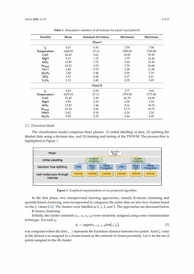
The classification model comprises three phases: (1) initial labelling of data, (2) splitting thelabeled data using a decision tree, and (3) training and testing of the TWSVM. The process flow ishighlighted in Figure 1.

Metals 2020, 10, x FOR PEER REVIEW 5 of 15

Table 1. Descriptive statistics of all features for plant I and plant II.

Variable Mean Standard Deviation Minimum Maximum

Plant I

𝒍𝒑 4.31 0.30 2.50 7.06

Temperature 1648.82 19.14 1500.00 1749.00

CaO 42.43 3.62 20.00 55.90

MgO 9.23 1.37 3.75 16.46

SiO2 12.89 1.74 5.40 23.30

Fetotal 18.22 3.53 7.70 36.00

MnO 4.80 0.70 2.28 11.98

Al2O3 1.80 0.48 0.59 7.79

TiO2 1.13 0.28 0.17 2.21

V2O5 2.13 0.49 0.25 3.95

Plant II

𝒍𝒑 4.63 0.34 2.77 5.64

Temperature 1679.10 27.11 1579.00 1777.00

CaO 53.45 2.30 42.33 64.06

MgO 0.99 0.34 0.30 3.18

SiO2 13.52 1.44 8.16 18.74

Fetotal 19.34 2.06 13.71 29.72

MnO 0.62 0.18 0.24 2.50

Al2O3 0.94 0.25 0.46 4.09

2.2. Theoretical Model

The classification model comprises three phases: (1) initial labelling of data, (2) splitting the

labeled data using a decision tree, and (3) training and testing of the TWSVM. The process flow is

highlighted in Figure 1.

In the first phase, two unsupervised learning approaches, namely K-means clustering and

quantile-based clustering, were incorporated to categorize the entire data set into four clusters based

on the 𝑙𝑝 values [26]. The clusters were labelled as 0, 1, 2, and 3. The approaches are discussed below.

K-means clustering:

Initially, the cluster centroids {𝑐1, 𝑐2, 𝑐3, 𝑐4} were randomly assigned using some randomization

technique. For each 𝑙𝑝,

𝑑𝑥 = arg min𝑗=1,2,3,4dist(𝑐𝑗 , 𝑙𝑝) (7)

was computed where the dist(. , . ) represents the Euclidean distance between two points. Each 𝑙𝑝

value in the dataset was assigned to a cluster based on the centroid of closest proximity. Let 𝑆𝑖 be the

set of points assigned to the 𝑖thcluster.

Figure 1. Graphical representation of our proposed algorithm. Figure 1. Graphical representation of our proposed algorithm.

In the first phase, two unsupervised learning approaches, namely K-means clustering andquantile-based clustering, were incorporated to categorize the entire data set into four clusters basedon the lp values [26]. The clusters were labelled as 0, 1, 2, and 3. The approaches are discussed below.

K-means clustering:Initially, the cluster centroids {c1, c2, c3, c4}were randomly assigned using some randomization

technique. For each lp,dx = argmin j=1,2, 3, 4dist

(c j, lp

)(7)

was computed where the dist(., .) represents the Euclidean distance between two points. Each lp valuein the dataset was assigned to a cluster based on the centroid of closest proximity. Let Si be the set ofpoints assigned to the ith cluster.

Metals 2020, 10, 25 6 of 15

The updated centroids {c′1, c′2, c′3, c′4}were calculated based on the mean of the clusters given as

c′i =1|Si|

∑j∈Si

lp, j (8)

The centroid update steps were carried out iteratively until a convergence condition was met.Typically, a convergence would mean that the relative difference between two consecutive steps wouldbe less than some small pre-specified quantity ε. Phase 1 of initial labelling of data using K-meansclustering is shown in Figure 2.

Metals 2020, 10, x FOR PEER REVIEW 6 of 15

The updated centroids {𝑐′1, 𝑐′2, 𝑐′3, 𝑐′4} were calculated based on the mean of the clusters given

as

𝑐′𝑖 = 1

|𝑆𝑖|∑ 𝑙𝑝,𝑗

𝑗∈𝑆𝑖

(8)

The centroid update steps were carried out iteratively until a convergence condition was met.

Typically, a convergence would mean that the relative difference between two consecutive steps

would be less than some small pre-specified quantity 𝜖. Phase 1 of initial labelling of data using K-

means clustering is shown in Figure 2.

Figure 2. K-means clustering for initial labelling of 𝑙𝑝 values.

Quantile-based clustering:

The second method used for initial labelling of 𝑙𝑝 values is based on quantiles (percentiles). Each

𝑙𝑝 was assigned to one of the four groups, viz. Minimum—25th percentile, 25th–50th percentile, 50th–

75th percentile, and 75th percentile—Maximum. Figure 3 shows an example of quartile-based

clustering of 𝑙𝑝 values.

Figure 3. Quantile-based clustering for initial labelling of 𝑙𝑝 values.

In the second phase of the algorithm, the labelled data was passed through a decision tree, with

two output nodes [25,26]. Three different criteria for splitting the decision tree were considered,

namely, Gaussian mixture models (GMM), mean shift (MS), and affinity propagation (AP) [26–30].

K-means clustering is developed on a deterministic idea that each data point can belong to only a

single cluster. However, GMM assumes that each data point has certain probabilities of belonging to

every cluster and that the data in each cluster follows a Gaussian distribution. The algorithm utilizes

e All clusters have equal data points

Figure 2. K-means clustering for initial labelling of lp values.

Quantile-based clustering:The second method used for initial labelling of lp values is based on quantiles (percentiles). Each lp

was assigned to one of the four groups, viz. Minimum—25th percentile, 25th–50th percentile, 50th–75thpercentile, and 75th percentile—Maximum. Figure 3 shows an example of quartile-based clustering oflp values.

Metals 2020, 10, x FOR PEER REVIEW 6 of 15

The updated centroids {𝑐′1, 𝑐′2, 𝑐′3, 𝑐′4} were calculated based on the mean of the clusters given

as

𝑐′𝑖 = 1

|𝑆𝑖|∑ 𝑙𝑝,𝑗

𝑗∈𝑆𝑖

(8)

The centroid update steps were carried out iteratively until a convergence condition was met.

Typically, a convergence would mean that the relative difference between two consecutive steps

would be less than some small pre-specified quantity 𝜖. Phase 1 of initial labelling of data using K-

means clustering is shown in Figure 2.

Figure 2. K-means clustering for initial labelling of 𝑙𝑝 values.

Quantile-based clustering:

The second method used for initial labelling of 𝑙𝑝 values is based on quantiles (percentiles). Each

𝑙𝑝 was assigned to one of the four groups, viz. Minimum—25th percentile, 25th–50th percentile, 50th–

75th percentile, and 75th percentile—Maximum. Figure 3 shows an example of quartile-based

clustering of 𝑙𝑝 values.

Figure 3. Quantile-based clustering for initial labelling of 𝑙𝑝 values.

In the second phase of the algorithm, the labelled data was passed through a decision tree, with

two output nodes [25,26]. Three different criteria for splitting the decision tree were considered,

namely, Gaussian mixture models (GMM), mean shift (MS), and affinity propagation (AP) [26–30].

K-means clustering is developed on a deterministic idea that each data point can belong to only a

single cluster. However, GMM assumes that each data point has certain probabilities of belonging to

every cluster and that the data in each cluster follows a Gaussian distribution. The algorithm utilizes

e All clusters have equal data points

Figure 3. Quantile-based clustering for initial labelling of lp values.

In the second phase of the algorithm, the labelled data was passed through a decision tree, withtwo output nodes [25,26]. Three different criteria for splitting the decision tree were considered, namely,Gaussian mixture models (GMM), mean shift (MS), and affinity propagation (AP) [26–30]. K-meansclustering is developed on a deterministic idea that each data point can belong to only a single cluster.However, GMM assumes that each data point has certain probabilities of belonging to every cluster and thatthe data in each cluster follows a Gaussian distribution. The algorithm utilizes expectation-maximization

Metals 2020, 10, 25 7 of 15

(EM) technique to estimate model parameters [27]. For a given data point, the algorithm estimates theprobability of belonging to a specific cluster and the point is assigned to the cluster for which this probabilityis maximum [28]. The next splitting algorithm, MS, clusters all the data points based on an attractionbasin with respect to convergence of a point to a cluster center [29]. This method is an unsupervisedlearning approach that iteratively shifts a data point towards the point of highest density or concentrationin the neighborhood. The number of clusters is not required to be specified as opposed to K-meansclustering. In Python, this algorithm is controlled by a parameter called the kernel bandwidth value whichgenerates a reasonable number of clusters based on the data. The final splitting algorithm tested was affinitypropagation [30]. Similar to MS, AP does not require to specify the number of clusters. This algorithmclusters points based on their relative attractiveness and availability. In the first step, the algorithm takesthe negative square difference feature by feature among all data points to produce a n× n similarity matrixS, where n is the number of data points. Similarity Function S(i, k) is defined as

S(i, k) = −‖xi − xk‖2 (9)

where i and k are the row and column indices, respectively. Based on this matrix, a n× n responsibilitymatrix R is generated by subtracting the similarity value between two data points, and then subtractingthe maximum of the remaining similarities. The responsibility matrix works as a helper matrix toconstruct the availability matrix A as

A(i, k)← S(i, k) − maxk′,k{A(i, k′) + S(i, k′)

}(10)

which indicates the relative availability of a data point to a particular cluster given the attractivenessreceived from the other clusters. In this matrix, the diagonal terms are updated using (12) and the restof the terms using (13) as

A(k, k) ←∑

i′ s.t. i′, k

max{0, R(i′, k)

}(11)

andA(i, k)← min{0, R(k, k) +

∑i′s.t. i′<{i,k}

max{0, R(i′, k)

}. (12)

The final step to create the clusters is by constructing a criterion matrix C, which is the sum of theavailability matrix and the responsibility matrix.

C(i, k)← R(i, k) + A(i, k) (13)

Subsequently, the highest value on each row is taken, and this value is known as the exemplar.Rows that share the same exemplar are in the same cluster where

exemplar(i, k) = max{A(i′, k) + R(i′, k)

}(14)

To generate the decision tree, one of the clustering algorithms was applied on the entire dataset toproduce two centroids acting as the basis for child nodes. The purpose of applying a cluster algorithmwas to find the optimal split of one node with four labels into two nodes with two labels each wherethe splitting criterion is the entropy among data points. For ease of computation, the initial clustersand child nodes are represented by their respective cluster centroids. This computation evaluates thedifference of each initial cluster centroid to each child node centroid, and the assignment is carried outbased on whichever combination produces the least entropy.

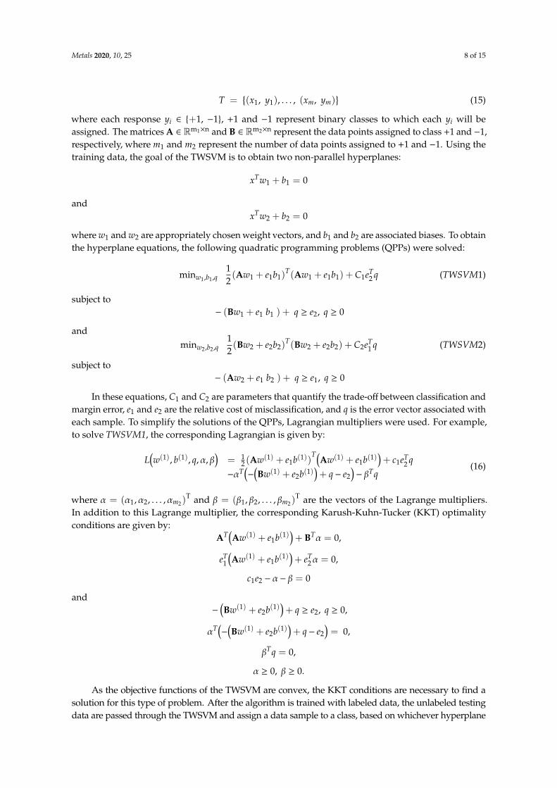
Once two children nodes are created with corresponding labels, they are passed through theTWSVM [22,23]. For generating the TWSVM, the data is split into 80% training and 20% testing data.A brief discussion on the working mechanism of TWSVM follows. Let x denote the feature vector andy denote the response variable. Let T be the training set:

Metals 2020, 10, 25 8 of 15

T ={(x1, y1), . . . , (xm, ym)

}(15)

where each response yi ∈ {+1, −1}, +1 and −1 represent binary classes to which each yi will beassigned. The matrices A ∈ Rm1×n and B ∈ Rm2×n represent the data points assigned to class +1 and −1,respectively, where m1 and m2 represent the number of data points assigned to +1 and −1. Using thetraining data, the goal of the TWSVM is to obtain two non-parallel hyperplanes:

xTw1 + b1 = 0

andxTw2 + b2 = 0

where w1 and w2 are appropriately chosen weight vectors, and b1 and b2 are associated biases. To obtainthe hyperplane equations, the following quadratic programming problems (QPPs) were solved:

minw1,b1,q12(Aw1 + e1b1)

T(Aw1 + e1b1) + C1eT2 q (TWSVM1)

subject to− (Bw1 + e1 b1 ) + q ≥ e2, q ≥ 0

andminw2,b2,q

12(Bw2 + e2b2)

T(Bw2 + e2b2) + C2eT1 q (TWSVM2)

subject to− (Aw2 + e1 b2 ) + q ≥ e1, q ≥ 0

In these equations, C1 and C2 are parameters that quantify the trade-off between classification andmargin error, e1 and e2 are the relative cost of misclassification, and q is the error vector associated witheach sample. To simplify the solutions of the QPPs, Lagrangian multipliers were used. For example,to solve TWSVM1, the corresponding Lagrangian is given by:

L(w(1), b(1), q,α, β

)= 1

2 (Aw(1) + e1b(1))T(

Aw(1) + e1b(1))+ c1eT

2 q−αT

(−

(Bw(1) + e2b(1)

)+ q− e2

)− βTq

(16)

where α = (α1,α2, . . . ,αm2)T and β = (β1, β2, . . . , βm2)

T are the vectors of the Lagrange multipliers.In addition to this Lagrange multiplier, the corresponding Karush-Kuhn-Tucker (KKT) optimalityconditions are given by:

AT(Aw(1) + e1b(1)

)+ BTα = 0,

eT1

(Aw(1) + e1b(1)

)+ eT

2α = 0,

c1e2 − α− β = 0

and−

(Bw(1) + e2b(1)

)+ q ≥ e2, q ≥ 0,

αT(−

(Bw(1) + e2b(1)

)+ q− e2

)= 0,

βTq = 0,

α ≥ 0, β ≥ 0.

As the objective functions of the TWSVM are convex, the KKT conditions are necessary to find asolution for this type of problem. After the algorithm is trained with labeled data, the unlabeled testingdata are passed through the TWSVM and assign a data sample to a class, based on whichever hyperplane

Metals 2020, 10, 25 9 of 15

is closer with respect to perpendicular distance. The accuracy of the final model is measured by theclassification rate (CR) which is the percentage of the test data correctly labeled. More specifically,

CR = n−14∑

i=1

aii

where aij is the number of heats with actual group label as ‘i’ (i = 1, 2, 3, 4) and predicted group labelas ‘j’ (j = 1, 2, 3, 4) in the test data and n =

∑4i=1

∑4j=1 aij. For our data, x represents the vector of slag

chemistry values corresponding to a particular heat and y takes −1 or +1 based on two classes of lp values.

2.3. Model Adequacy

Five-fold cross-validation was applied to the model. This is a resampling procedure used toevaluate the machine learning model performance on the training data. Following this procedure,the results were less biased towards an arbitrary selection of the test set. In the five-fold cross-validationstep, the dataset is split into five groups, so that the model is trained four times with one group beingheld up from the training set and used as a test set. In this manner, each group has the opportunity tobe the test set once, and therefore, the bias of the model is reduced. The final accuracy presented in theresults section is an average of the four accuracies values obtained in the five-fold cross-validation step.Finally, in both plants the data points were normalized to reduce the amount of computational powerneeded to train and keep the data entropy in the same order of magnitude among all features.

3. Results

3.1. Descriptive Statistics

Mean, standard deviation (SD), minimum and maximum for the set of features (i.e., slag chemistrycomponents), and lp values are presented in Table 1. Box plots for all the features and lp value for plantI are presented in Figure 4. To maintain brevity, the box plots corresponding to the features for plant IIare not provided. The box plots indicate that most of the features have symmetric distribution exceptFetotal, MnO and Al2O3. These plots serve as a visual aid to identify the range of values containing themiddle 50% of the data for each feature. For example, the longer whisker of the box plot correspondingto Al2O3 indicates that the values are skewed and potentially have many outliers, while the middle50% lies between 1.5% and 2% by weight. Table 2 shows the distribution of the lp values in each of theinitially labeled clusters by K-means for both plant I and plant II. It is observed that each cluster has adistinct range of lp values since there is no overlap among one standard deviation intervals from themean. For quantile-based clustering, each cluster has approximately 3563 (25%) observations for plantI and 771 (25%) observations for plant II. This signifies that the initial cluster labels have the potentialto classify lp values into disjoint intervals, and therefore, could be a reliable measurement to categorizefeatures based on the degree of dephosphorization.

Table 2. Classification of lp based on the labels from K-means clustering for plant I and plant II.

Cluster Label Frequency (%) Mean Standard Deviation Minimum Maximum

Plant I

0 2711 (19.57) 3.76 0.16 2.50 3.941 5316 (38.37) 4.12 0.09 3.94 4.262 4338 (31.31) 4.41 0.08 4.26 4.563 1488 (10.75) 4.72 0.14 4.56 7.06

Plant II

0 1364 (44.23) 3.66 0.56 2.77 3.991 1029 (33.37) 4.30 0.13 3.99 4.492 584 (18.94) 4.68 0.10 4.49 4.853 107 (3.46) 4.99 0.11 4.85 5.64

Metals 2020, 10, 25 10 of 15

Metals 2020, 10, x FOR PEER REVIEW 10 of 15

3.2. Model Hyper-parameter Selection

The model hyper-parameters are parameters that cannot be learnt by the model during the

training phase. Hyper-parameters are supplied to the model by the user and tuned empirically, in

most cases, by a trial and error approach. The performance of the model is heavily dependent on our

choice of hyper-parameters since they influence how fast the model learns and converges to a

solution. For Twin-SVM, those hyper-parameters are epsilon (𝜖) and the cost (𝐶) function as defined

in Section 2. 𝜖 regulates the distance from the boundary decision layer to the threshold at which a

point belonging to a certain class and within the threshold should be penalized by the cost function.

Consequently, the larger the cost function the higher the penalty for a point within the threshold. A

large 𝜖 will hinder the model convergence whereas a smaller 𝜖 may cause an over-fitted decision

boundary. Other hyper-parameters also determine the model’s ability to construct a linear or non-

linear structure. TWSVM can accommodate linear, polynomial, and radial basis function (RBF)

kernels. These kernels are transformations applied onto the dataset to produce a representation of

these data in a different space where feature sets can be classified [25,26].

The hyper-parameters where selected using a trial and error approach, with the starting values,

increments, and ending values presented in Table 3. From this table, the selected hyper parameter

based on best performance in terms of accuracy was selected. The trial and error approach though is

not random but considered following the best practices in the field of machine learning. A

comparison between Linear and RBF kernel-based DT2-SVM-KC was carried out. RBF performed

better than the linear kernel-based TWSVM in terms of accuracy (classification rate), which further

indicates the strong presence of inherent non-linearity in the data obtained in BOF steelmaking. A

third option considered was a polynomial kernel; however, it was not considered because it resulted

in computational overflowing even for a quadratic polynomial.

3.3. Accuracy of Results

The results of the analysis of BOF data based on decision tree twin SVM cluster-based algorithm

are presented in this section. As mentioned previously, two methods of labeling 𝑙𝑝 values: quartiles-

based and K-means-based, along with three clustering algorithms function as split criterion for the

decision tree to give a total of six different DT2-SVM-KC algorithms. The accuracy (%) for each of

these algorithms is presented in Table 4.

Figure 4. Box plots of all features and the response variable for plant I data.

Figure 4. Box plots of all features and the response variable for plant I data.

3.2. Model Hyper-Parameter Selection

The model hyper-parameters are parameters that cannot be learnt by the model during thetraining phase. Hyper-parameters are supplied to the model by the user and tuned empirically,in most cases, by a trial and error approach. The performance of the model is heavily dependenton our choice of hyper-parameters since they influence how fast the model learns and convergesto a solution. For Twin-SVM, those hyper-parameters are epsilon (ε) and the cost (C) function asdefined in Section 2. ε regulates the distance from the boundary decision layer to the threshold atwhich a point belonging to a certain class and within the threshold should be penalized by the costfunction. Consequently, the larger the cost function the higher the penalty for a point within thethreshold. A large ε will hinder the model convergence whereas a smaller ε may cause an over-fitteddecision boundary. Other hyper-parameters also determine the model’s ability to construct a linear ornon-linear structure. TWSVM can accommodate linear, polynomial, and radial basis function (RBF)kernels. These kernels are transformations applied onto the dataset to produce a representation ofthese data in a different space where feature sets can be classified [25,26].

The hyper-parameters where selected using a trial and error approach, with the starting values,increments, and ending values presented in Table 3. From this table, the selected hyper parameterbased on best performance in terms of accuracy was selected. The trial and error approach though isnot random but considered following the best practices in the field of machine learning. A comparisonbetween Linear and RBF kernel-based DT2-SVM-KC was carried out. RBF performed better thanthe linear kernel-based TWSVM in terms of accuracy (classification rate), which further indicatesthe strong presence of inherent non-linearity in the data obtained in BOF steelmaking. A thirdoption considered was a polynomial kernel; however, it was not considered because it resulted incomputational overflowing even for a quadratic polynomial.

Metals 2020, 10, 25 11 of 15

Table 3. Selection of Hyper-parameters for SVM for plant I and plant II.

Hyperparameter Starting Value Increments Ending Value Selected Parameter(Plant I)

Selected Parameter(Plant II)

ε1 0.1 0.1 2.0 0.4 0.5ε2 0.1 0.1 2.0 0.5 0.5C1 0.1 0.1 2.5 1 1C2 0.1 0.1 2.5 1 1

Kernel Type Linear N/A Radial Radial RadialKernel Parameter 0.5 0.1 3.0 2.5 2

3.3. Accuracy of Results

The results of the analysis of BOF data based on decision tree twin SVM cluster-based algorithm arepresented in this section. As mentioned previously, two methods of labeling lp values: quartiles-basedand K-means-based, along with three clustering algorithms function as split criterion for the decisiontree to give a total of six different DT2-SVM-KC algorithms. The accuracy (%) for each of thesealgorithms is presented in Table 4.

Table 4. Accuracy results of the DT2-SVM-KC algorithm for both plants.

Labelling Method GMM Mean Shift Affinity Propagation

Plant I Accuracy

K-Means 78.76% 71.77% 72.00%Quartile 64.38% 62.35% 62.79%

Plant II Accuracy

K-Means 98.03% 98.01% 96.58%Quartile 95.78% 94.81% 94.00%

A five-fold cross-validation technique was applied to validate the model adequacy. Of the six casesmentioned in Table 5, K-means clustering as a label generator and GMM-cluster-based DT2-SVM-KC,provided the most accurate result with accuracy around 98.03%.

Table 5. Accuracy comparison between SVM vs. TWSVM with Decision Trees for K-means clusteringas the initial label generator.

Labelling Method GMM Mean Shift Affinity Propagation

Plant I Accuracy

TWSVM 78.76% 71.77% 72.00%SVM 72.97% 74.79% 76.11%

Plant II Accuracy

TWSVM 98.03% 98.01% 96.58%SVM 97.45% 98.00% 96.42%

A comparison between GMM, MS and AP-based algorithm is presented Figure 5. Results showthat GMM performed better than MS and AP in terms of accuracy for each dataset. Figure 6 showsthe accuracy obtained using K-Means clustering vs. quartile clustering to generate initial labels oflp. This figure shows that K-Means clearly yield a superior accuracy when examined against thequartile-based clustering method. The mean of the accuracy across the node-leaves for plant I is 78.77%and for plant II is 98.04%.

Metals 2020, 10, 25 12 of 15

Metals 2020, 10, x FOR PEER REVIEW 11 of 15

Table 3. Selection of Hyper-parameters for SVM for plant I and plant II.

Hyperparameter Starting

Value Increments

Ending

Value

Selected Parameter

(Plant I)

Selected Parameter

(Plant II)

𝜖1 0.1 0.1 2.0 0.4 0.5

𝜖2 0.1 0.1 2.0 0.5 0.5

𝐶1 0.1 0.1 2.5 1 1

𝐶2 0.1 0.1 2.5 1 1

Kernel Type Linear N/A Radial Radial Radial

Kernel Parameter 0.5 0.1 3.0 2.5 2

Table 4. Accuracy results of the DT2-SVM-KC algorithm for both plants.

Labelling Method GMM Mean Shift Affinity Propagation

Plant I Accuracy

K-Means 78.76% 71.77% 72.00%

Quartile 64.38% 62.35% 62.79%

Plant II Accuracy

K-Means 98.03% 98.01% 96.58%

Quartile 95.78% 94.81% 94.00%

A five-fold cross-validation technique was applied to validate the model adequacy. Of the six

cases mentioned in Table 5, K-means clustering as a label generator and GMM-cluster-based DT2-

SVM-KC, provided the most accurate result with accuracy around 98.03%.

A comparison between GMM, MS and AP-based algorithm is presented Figure 5. Results show

that GMM performed better than MS and AP in terms of accuracy for each dataset. Figure 6 shows

the accuracy obtained using K-Means clustering vs. quartile clustering to generate initial labels of 𝑙𝑝.

This figure shows that K-Means clearly yield a superior accuracy when examined against the quartile-

based clustering method. The mean of the accuracy across the node-leaves for plant I is 78.77% and

for plant II is 98.04%.

Figure 5. A comparison among the accuracy results of GMM, Mean Shift and Affinity Propagation

using K-Means as the initial labeling method.

3.4. Justification for Twin SVM over other SVM models

To validate the use of a complex model such as Twin SVM, we compare its results with general

SVM-based models. Results are shown in Figure 7. Further, Table 5 shows that twin SVM improves

the accuracy of the binary classification problem by at least 15% for both plants I and II. The hyper-

parameters for the SVM were tuned to reach maximum possible accuracy and the decision tree was

consistent with the best method used with Twin SVM (i.e., K-means as labeling generator and GMM

as splitting criterion for the decision tree).

Figure 5. A comparison among the accuracy results of GMM, Mean Shift and Affinity Propagationusing K-Means as the initial labeling method.

Metals 2020, 10, x FOR PEER REVIEW 12 of 15

Figure 6. A comparison between the accuracy results of K-Means and quartile-based clustering using

GMM as the splitting criterion.

Table 5. Accuracy comparison between SVM vs. TWSVM with Decision Trees for K-means clustering

as the initial label generator.

Labelling Method GMM Mean Shift Affinity Propagation

Plant I Accuracy

TWSVM 78.76% 71.77% 72.00%

SVM 72.97% 74.79% 76.11%

Plant II Accuracy

TWSVM 98.03% 98.01% 96.58%

SVM 97.45% 98.00% 96.42%

Figure 7. A comparison between accuracy results of SVM vs. TWSVM-based models.

4. Discussion and Interpretation of Results

In this section, the results of the analysis are discussed. This section comprises of two parts. First,

a discussion about the performance of the algorithm, and second, an interpretation from an industrial

perspective.

4.1. Algorithm Performance

Twin SVM outperforms SVM by at least 15% across all datasets. Mathematically, twin SVM

solves two smaller quadratic programming problems rather than a larger one as SVM does.

Therefore, twin SVM is tailored for binary classification, which also means that the decision tree

boosts its accuracy. This is because the decision tree reduces a multi-class classification problem into

small binary problems that can be solved by the twin SVM. In fact, the decision tree allows a greater

Figure 6. A comparison between the accuracy results of K-Means and quartile-based clustering usingGMM as the splitting criterion.

3.4. Justification for Twin SVM over Other SVM Models

To validate the use of a complex model such as Twin SVM, we compare its results withgeneral SVM-based models. Results are shown in Figure 7. Further, Table 5 shows that twinSVM improves the accuracy of the binary classification problem by at least 15% for both plants I and II.The hyper-parameters for the SVM were tuned to reach maximum possible accuracy and the decisiontree was consistent with the best method used with Twin SVM (i.e., K-means as labeling generator andGMM as splitting criterion for the decision tree).

Metals 2020, 10, x FOR PEER REVIEW 12 of 15

Figure 6. A comparison between the accuracy results of K-Means and quartile-based clustering using

GMM as the splitting criterion.

Table 5. Accuracy comparison between SVM vs. TWSVM with Decision Trees for K-means clustering

as the initial label generator.

Labelling Method GMM Mean Shift Affinity Propagation

Plant I Accuracy

TWSVM 78.76% 71.77% 72.00%

SVM 72.97% 74.79% 76.11%

Plant II Accuracy

TWSVM 98.03% 98.01% 96.58%

SVM 97.45% 98.00% 96.42%

Figure 7. A comparison between accuracy results of SVM vs. TWSVM-based models.

4. Discussion and Interpretation of Results

In this section, the results of the analysis are discussed. This section comprises of two parts. First,

a discussion about the performance of the algorithm, and second, an interpretation from an industrial

perspective.

4.1. Algorithm Performance

Twin SVM outperforms SVM by at least 15% across all datasets. Mathematically, twin SVM

solves two smaller quadratic programming problems rather than a larger one as SVM does.

Therefore, twin SVM is tailored for binary classification, which also means that the decision tree

boosts its accuracy. This is because the decision tree reduces a multi-class classification problem into

small binary problems that can be solved by the twin SVM. In fact, the decision tree allows a greater

Figure 7. A comparison between accuracy results of SVM vs. TWSVM-based models.

Metals 2020, 10, 25 13 of 15

4. Discussion and Interpretation of Results

In this section, the results of the analysis are discussed. This section comprises of two parts.First, a discussion about the performance of the algorithm, and second, an interpretation from anindustrial perspective.

4.1. Algorithm Performance

Twin SVM outperforms SVM by at least 15% across all datasets. Mathematically, twin SVM solvestwo smaller quadratic programming problems rather than a larger one as SVM does. Therefore, twinSVM is tailored for binary classification, which also means that the decision tree boosts its accuracy.This is because the decision tree reduces a multi-class classification problem into small binary problemsthat can be solved by the twin SVM. In fact, the decision tree allows a greater number of classes aslong as the node-leaves end up with two classes (i.e., 2k where k ≥ 2). The downside of increasing thenumber of classes is that each node-leaf will have less data points to train every time we increase thenumber of classes resulting in less significant and biased results. Given the number of data points,empirically, four classes were found to be optimal for this experiment.

With regards to the difference in accuracy across plants, it is worth noticing that although plant Ihas five times more data points than plant II, the accuracy in plant I is lower. This is counter intuitive;however, two possible attributive factors could be suggested. First, that plant I has more features (i.e.,V2O5 and TiO2) than plant II, and, second, the range in lp values from plant II is shorter than the onefrom plant I as shown in Table 1. As a consequence, the classification for plant I is more difficult due tohigher variability of the data. On the other hand, ore from plant I contains more phosphorus thanin plant B, which further plays role in the reduction of accuracy for plant I data. What such resultssuggest is that the tuning of hyper-parameters should be performed distinctively on each plant data;nevertheless, the algorithm will remain the same.

Finally, as part of the data pre-processing stage, all data points were normalized. The purposeof normalizing the data was to reduce the computational power for training and testing.Unexpectedly, normalizing also had an effect on the accuracy of the algorithm since an incrementof at least 3 percentage points was noted for both plants. This effect was also attributed to the factthat less variability increases the accuracy of the machine-learning model. By normalizing the data,the influence of features with high numerical values such as temperature are weighted the same as theinfluence of other features with less numerical values such as MnO or CaO.

4.2. Application of the Results for Industry

From an industrial view point, the method of initial labeling is crucial. It means, given certainslag chemistry, we can predict the percentage of phosphorus in the steel. K-means clustering labels thedata based on the proximity of an unlabeled data point to the cluster center of labeled data points.This center will be dynamically updated until the algorithm converges but it always represents themean of data points within the cluster at any given time. For a metallurgist, the results of the algorithmwill show how close the current batch is to a certain lp value (i.e., center of the cluster). The advantageof using K-means over quartiles labelling approach is clearly demonstrated in terms of accuracy asillustrated in Table 5. One explanation for such results is that K-means is grouped-based clusteringwhile quartiles labeling considers only the relative position of a value with respect to the others.

The GMM cluster-based decision tree TWSVM algorithm designed in this research aims forattaining higher flexibility and adaptability to real world conditions. Given the values of slag chemistryfor a particular heat in a BOF shop, our model will be able to predict to which of the four lp classes (i.e.,0–3), the batch will fall. For example, if the current batch belongs to class-0, the content of phosphorusin the resulting steel will be high and the corresponding output will be undesirable. The objective isto produce steel corresponding to high lp classes (class 2–3). The proposed algorithm has proven towork seamlessly with two different plants having different slag chemistries. The algorithm provides a

Metals 2020, 10, 25 14 of 15

general framework and requires training data from a specified plant in order to achieve the optimalaccuracy results for classifying lp values.

5. Conclusions

A decision tree twin support vector machine based on a kernel clustering (DT2-SVM-KC)machine-learning model is proposed in this paper. The model classifies a batch (obtained froma specific heat at a BOF shop) based on slag chemistries into one of the four classes of lp values.Class 0 corresponds to highest phosphorus content in the resulting output while class 3 corresponds tolowest phosphorus content in the resulting steel. The model is efficient and shows high accuracy witha relatively low computational requirement and cost. Even though further testing on different datasetsis required, the model has shown consistent performance across Plant I and II. However, it was noticedthat with an increase in the number of features and variability of the response variable lp, the accuracyof the algorithm decreases. So, it is recommended that a metallurgical model based on fundamentaltheory might be helpful in ruling out features that do not necessarily affect or have negligible influenceon the amount of phosphorus in the steel. Additionally, it is recommended that for samples with highvariability in the response variable ( lp), an increase in the number of labels during the cluster labellingcould be advantageous given there are enough data points corresponding to each node leaf. This is toavoid an under fitted model with unreliable results.

Finally, one of the main considerations towards industry applications is the interpretability ofthese results. In this paper, the results suggest that given a data point from a heat, one can deduct acertain lp range for that batch and also understand the influence of the features on the results suchthat the slag composition can be tweaked to reduce the amount of phosphorus in liquid steel for thenext batch.

Author Contributions: K.C. conceptualized the assessment of machine-learning techniques on dephosphorizationdata. S.B. conceptualized the use of the decision tree twin support vector machine algorithm. K.C. provided theacquired data via two steel plants. J.P. and J.E. performed various statistical analysis on the data. K.C. providedfunding of the project. J.E. and J.P. designed and developed the algorithms, as well as implemented in on Python.S.B. provided mentorship of the project. J.P. created the figures in the paper. J.P. and J.E. wrote the initial draft ofthe manuscript. S.B. and S.M. edited and critically reviewed the final manuscript. All authors have read andagreed to the published version of the manuscript.

Funding: This research received no external funding.

Conflicts of Interest: The authors declare no conflict of interest.

References

1. Iron Ore Monthly Price-US Dollars per Dry Metric Ton. Available online: https://www.indexmundi.com/

commodities/?commodity=iron-ore (accessed on 10 July 2019).2. Bloom, T. The Influence of Phosphorus on the Properties of Sheet Steel Products and Methods Used to

Control Steel Phosphorus Level in Steel Product Manufacturing. Iron Steelmak. 1990, 17, 35–41.3. Chukwulebe, B.O.; Klimushkin, A.N.; Kuznetsov, G.V. The utilization of high-phosphorous hot metal in BOF

steelmaking. Iron Steel Technol. 2006, 3, 45–53.4. Urban, D.I.W.; Weinberg, I.M.; Cappel, I.J. De-phosphorization strategies and Modeling in Oxygen

Steelmaking. Iron Steel Technol. 2014, 134, 27–39.5. Balajiva, K.; Quarrell, A.; Vajragupta, P. A laboratory investigation of the phosphorus reaction in the basic

steelmaking process. J. Iron Steel Inst. 1946, 153, 115.6. Turkdogan, E.; Pearson, J. Activities of constituents of iron and steelmaking slags. ISIJ 1953, 175, 398–401.7. Suito, H.; Inoue, R. Thermodynamic assessment of hot metal and steel dephosphorization with

MnO-containing BOF slags. ISIJ Int. 1995, 35, 258–265. [CrossRef]8. Healy, G. New look at phosphorus distribution. J. Iron Steel Inst. 1970, 208, 664–668.9. Turkdogan, E. Slag composition variations causing variations in steel dephosphorisation and desulphurisation

in oxygen steelmaking. ISIJ Int. 2000, 40, 827–832. [CrossRef]

Metals 2020, 10, 25 15 of 15

10. Chattopadhyay, K.; Kumar, S. Application of thermodynamic analysis for developing strategies to improveBOF steelmaking process capability. In Proceedings of the AISTech 2013 Iron and Steel Technology Conference,Pittsburgh, PA, USA, 6–9 May 2013; pp. 809–819.

11. Drain, P.B.; Monaghan, B.J.; Zhang, G.; Longbottom, R.J.; Chapman, M.W.; Chew, S.J. A review of phosphoruspartition relations for use in basic oxygen steelmaking. Ironmak. Steelmak. 2017, 44, 721–731. [CrossRef]

12. Kitamura, S.; Kenichiro, M.; Hiroyuki, S.; Nobuhiro, M.; Michitaka, M. Analysis of dephosphorizationreaction using a simulation model of hot metal dephosphorization by multiphase slag. ISIJ Int. 2009, 49,1333–1339. [CrossRef]

13. Kitamura, S.; Kimihisa, I.; Farshid, P.; Masaki, M. Development of simulation model for hot metaldephosphorization process. Tetsu Hagane J. Iron Steel Inst. Jpn. 2014, 100, 491–499. [CrossRef]

14. Chatterjee, S.; Hadi, A.S. Regression Analysis by Example; John Wiley & Sons: New York, NY, USA, 2015.15. Kloke, J.; McKean, J.W. Nonparametric Statistical Methods Using R; Chapman and Hall/CRC: Boca Raton, FL,

USA, 2014.16. Wang, Z.; Xie, F.; Wang, B.; Liu, Q.; Lu, X.; Hu, L.; Cai, F. The control and prediction of end-point phosphorus

content during BOF steelmaking process. Steel Res. Int. 2014, 85, 599–606. [CrossRef]17. He, F.; Zhang, L. Prediction model of end-point phosphorus content in BOF steelmaking process based on

PCA and BP neural network. J. Process Control 2018, 66, 51–58. [CrossRef]18. Barui, S.; Mukherjee, S.; Srivastava, A.; Chattopadhyay, K. Understanding dephosphorization in basic oxygen

furnaces (BOFs) using data driven modeling techniques. Metals 2019, 9, 955. [CrossRef]19. Wang, X.; Han, M.; Wang, J. Applying Input Variables Selection Technique on Input Weighted Support Vector

Machine Modeling for BOF Endpoint Prediction. Eng. Appl. Artif. Intell. 2010, 23, 1012–1018. [CrossRef]20. Liu, C.; Tang, L.; Liu, J.; Tang, Z. A dynamic analytics method based on multistage modeling for a BOF

steelmaking process. IEEE Trans. Autom. Sci. Eng. 2018, 16, 1097–1109. [CrossRef]21. Gao, C.; Shen, M.; Liu, X.; Wang, L.; Chen, M. End-point prediction of BOF steelmaking based on KNNWTSVR

and LWOA. Trans. Indian Inst. Met. 2018, 72, 257–270. [CrossRef]22. Dou, Q.; Zhang, L. Decision tree twin support vector machine based on kernel clustering for multi-class

classification. In Proceedings of the International Conference on Neural Information Processing, Siem Reap,Cambodia, 13–16 December 2018; pp. 293–303.

23. Khemchandani, R.; Chandra, S. Twin support vector machines for pattern classification. IEEE Trans.Pattern Anal. Mach. Intell. 2007, 29, 905–910.

24. Ding, S.; Yu, J.; Qi, B.; Huang, H. An overview on twin support vector machines. Artif. Intell. Rev. 2014, 42,245–252. [CrossRef]

25. James, G.; Witten, D.; Hastie, T.; Tibshirani, R. An Introduction to Statistical Learning; Springer Science +

Business Media: New York, NY, USA, 2013.26. Friedman, J.; Hastie, T.; Tibshirani, R. The Elements of Statistical Learning; Springer Series in Statistics; Springer:

New York, NY, USA, 2001.27. McLachlan, G.; Krishnan, T. The EM Algorithm and Extensions; John Wiley & Sons: New York, NY, USA, 2007.28. Carrasco, Oscar. Gaussian Mixture Models Explained. Available online: https://towardsdatascience.com/

gaussian-mixture-models-explained-6986aaf5a95 (accessed on 1 August 2019).29. Comaniciu, D.; Meer, P. Mean Shift: A Robust Approach toward Feature Space Analysis. IEEE Trans.

Pattern Anal. Mach. Intell. 2002, 24, 603–619. [CrossRef]30. Frey, B.J.; Dueck, D. Clustering by passing messages between data points. Science 2007, 315, 972–976.

[CrossRef] [PubMed]

© 2019 by the authors. Licensee MDPI, Basel, Switzerland. This article is an open accessarticle distributed under the terms and conditions of the Creative Commons Attribution(CC BY) license (http://creativecommons.org/licenses/by/4.0/).