time consistent policy in markov switching models∗ - repec
TRANSCRIPT

Time Consistent Policy in Markov SwitchingModels∗
Andrew P. Blake and Fabrizio ZampolliBank of England
First draft: February 25, 2004This draft: August 30, 2005
Abstract
In this paper we consider the optimal control problem of modelswith Markov regime shifts and forward looking agents. These modelsare general and flexible tools for modelling model uncertainty. Analgorithm is devised to compute the solution of a rational expectationsmodel with random parameters or regime shifts. A second algorithmcomputes the time consistent policy and the resulting Nash Stackelbergequilibrium. The latter algorithm can also handle the case in whichthe policymaker and the private sector hold different beliefs. We applythese methods to compute the optimal (nonlinear) monetary policy ina small open economy subject to random structural breaks.
1 Introduction
Uncertainty is one of the considerable problems faced by economic policy-makers. It surrounds observed data, unobserved expectations and potentialequilibria as well as both the structure and parameters of the economy. Evenif models are subject to quantifiable risk, this can have a substantial impacton the formulation of optimal economic policies. A considerable amount ofrecent research has been directed at countering these and various sources ofuncertainty.1
In this paper we focus on one such quantifiable risk, one in which theeconomy is subject to regime shifts with the particular regime followed be-ing determined by a Markov process. This set up can be thought of as
∗Earlier versions of this paper was presented at the Selected Economists’ Workshop,Centre for Central Bank Studies, Bank of England, September 2004 and the Society forComputational Economics Conference, Washington, D.C., May 2005. We are grateful toconference participants and two referees for many useful comments.
1See, in a completely arbitrary but recent list, Kozicki (2004); Swanson (2004); Planasand Rossi (2004).
1

encompassing a number of possible representations of the world. It can beviewed as a model with stochastic parameters or perhaps a model in whichagents learning is characterised as a jump process. This latter set up canbe particularly useful for models where bubble-like behaviour is observed.A collapsed bubble is one where sufficient agents feel it is unsustainable.
The economic policy problem is pervasive in such a world. For anymodel, particularly a stochastic one, we need to decide what form of policyrule we should implement and together with rational, forward-looking agentswe need to consider the appropriate treatment of expectations in the optimalpolicy problem. In this paper we adopt a game-theoretic framework for thedesign of optimal policy. In particular we seek policies which are both timeconsistent and subgame perfect, following Fershtman (1989): Policies needto both be consistent and take into account the stochastic nature of theproblem. The time consistency restriction rules out policymakers adoptingpolicies which are ex ante likely to become sub optimal simply because timepasses, and are therefore unsustainable as a description of credible a policy.Both considerations require us to consider solutions derived by dynamicprogramming rather than Lagrange multipliers: We need a ‘rule’ for agents’expectations, not a time path for future actions (Basar and Olsder, 1999).
This is particularly appropriate in our case. We adopt a recursive ap-proach to optimal policy formulation with Markov-switching parameters.Such an approach necessarily imposes time consistency via the principle ofoptimality. If the model itself is subject to change, why should policymak-ers actions be immune? We therefore rule out potentially time inconsistentbehaviour through our recursive formulation.
To do this we develop algorithms both for the solution of rational ex-pectations models with probabalistically-driven regime changes and for theoptimal time-consistent subgame-perfect control of such models. The controlsolution adopted in Zampolli (2005) is adapted to provide the best policy.2
We also show how these algorithms can be modified to allow the policy-makers and private agents to hold different beliefs over the probability ofa regime shift. These methods are applied to a small open economy modeldeveloped by e.g. Batini and Nelson (2000) and Leitemo and Söderström(2004) to investigate structural changes in agent behaviour. These can bothbe characterised as a form of learning. In Appendix A we develop the samemethods in a form consistent with Oudiz and Sachs (1985) rather than thesemi-structural form used in the main part of the paper (see Dennis andSöderström (2002)).
Whilst our focus is on time consistency, it should be noted that therational expectations solution we develop could be used for any arbitrary
2In the engineering literature, Aoki (1967) studied the control of regime-shifting models.These models are currently referred to in this literature as Markov Jump Linear Systems(MJLS). For recent contributions, see Costa et al. (2005).
2

policy rules, such as a Taylor rule, and the optimal time inconsistent policycould be obtained using very similar methods. There are difficulties withtime inconsistent policy in this context however, as any change in policy mustbe in response only to news about changes in regime rather than potentialwelfare improvements from reneging. This means that the implications ofany inherited part of policy for a new regime could be extremely bad, andpolicymakers would never want to carry them out even if the consequencesof a loss of reputation were severe. We focus on time consistency to removethis possibility.
The paper is organised as follows. Section 2 provides the underminedcoefficient model solution to a rational expectation model with regime shifts.This solution forms the basis for solving the optimal control problem which isdealt with in Section 3. Section 4 describes the small open economy modelused in the application and the experiments being carried out. Section 5describes how to simulate the model both under symmetric and asymmetricbeliefs. Section 6 presents the results of the application. Section 7 concludes.
2 Undetermined coefficient model solution withregime shifts
We consider a linear rational expectations model in semi-structural form:
xt = A(st)xt−1 +B(st)E [xt+1|It] +C(st)εt (1)
where x is a vector of variables that can depend on lags and leads, A(st),B(st) and C(st) are stochastic matrices which will depend on regime st ∈{1, 2, ...N} and E [εt+1|It] = 0 is a vector of stochastic shocks with It theinformation set at time t. The dominant regime will be determined by aMarkov process. This model is described as semi-structural as it distin-guishes between leads and lags for each potential equation, although forlonger leads and lags the model would need to be augmented. By contrastthe state space form (Appendix A) requires classification of the variables bytype (jump or predetermined).
The model can be solved depending on agent’s expectations of futurepolicy regimes. Let the assumed reduced-form law of motion be:
xt = D(st)xt−1 + F (st)εt (2)
where D(·) and F (·) are matrices of undetermined coefficients and we havesolved out for expectations. For simplicity we assume that there are onlytwo states. The formulae are easily generalised to the N-state case (seeAppendix A, for example).
3

To find the unknown coefficients, first solve for the expectation:
E [xt+1|It] = E [D(st+1)xt + F (st+1)εt+1|It]= E [D(st+1)|It]xt +E [F (st+1)|It]E [εt+1|It]= E [D(st+1)|It]xt= (pi1D1 + pi2D2)xt
≡ Dixt
= Di (Dixt−1 + Fiεt)
= DiDixt−1 + DiFiεt
where i denotes the regime at time t, i.e. st = i. Now plugging the aboveexpression back into the model gives:
xt = Aixt−1 +Bi
¡DiDixt−1 + DiFiεt
¢+Ciεt
=¡Ai +BiDiDi
¢xt−1 +
¡BiDiFi +Ci
¢εt. (3)
Given the assumed law of motion, xt = Dixt−1 + Fiεt, the undeterminedcoefficients must satisfy the following conditions:
Di = Ai +BiDiDi (4)
Fi = BiDiFi +Ci (5)
for i = 1, ...N . The first set of equations are to be solved for the feedbackpart of the solution, Di:
Di = Ai +BiDiDi
= Ai +Bi (pi1D1 + pi2D2)Di.
So, for i = 1:
D1 = A1 +B1 (p11D1 + p12D2)D1
= A1 +B1p11D21 +B1p12D2D1
0 = B1p11D21 + (B1p12D2 − I)D1 +A1
Likewise for i = 2. This yields a pair of coupled equations that need to besolved simultaneously:
0 = B1p11D21 + (B1p12D2 − I)D1 +A1 (6)
0 = B2p22D22 + (B2p21D1 − I)D2 +A2. (7)
These equations can be solved iteratively, if a solution exists3 using an ap-propriate solution method. Given a procedure for solving matrix quadraticequations, we can solve the linked equations sequentially. The following isa possible solution algorithm for the two-state case. It generalises easily forthe multi-state model.4
3There are few proofs about the existence of solutions to such problems. We considerthis to be a useful avenue for future research, as, in our experience, solution methods canfail for interesting and plausible economic models.
4As with the control solutions below we have implemented the solutions in Matlabtm.
4

Algorithm 1 Rational solution with Markov switching (two-state case).For the model (1) assume a solution of the form (2).
1. Select initial values for D0 =¡D01, D
02
¢.
2. Solve quadratic equations for given values of Dr, obtaining a new setDr+1:
Dr+11 = g(B1p11, B1p12D
r2 − I, A1)
Dr+12 = g(B2p22, B2p21D
r1 − I, A2)
where g(·) is a quadratic equation solver for (6) and (7). Similarlysolve F .
3. Check convergence: if¯Dr+1
¯< ε or too many iterations stop; else
repeat 2.
There are some issues to consider. First, in the standard case the rootsof the single quadratic equation can be checked and it can be establishedif there are determinate, indeterminate or no solutions. In our linked casethis is no longer possible. If a solution exists and can be found by thisprocedure, we can check whether the solution is stable conditional on theother Riccati solution(s). As mentioned above, issues of existence have notbeen established in this class of model and time consistent policy problem.
Second, if the model incorporates the optimal policy rule, is this solutionstabilising and unique? In the linear-quadratic optimal control problem, itis. What about in this non-standard case? Again, results do not currentlyexist, but we have so far been able to find solutions using our suggestedalgorithms.
Third, we can easily adapt this as a method for solving for an optimalfixed parameter policy rule. Given that we have a rational expectationssolution we could simply impose a fixed parameter policy rule and optimiseover the coefficients to find the best Taylor-type rule, for example. Sucha policy would likely vary depending on the initial regime. A min-maxapproach could yield a rule that was best given any initial regime.
In the next section we turn to the optimal control problem, which relieson the reduced form solutions obtained here.
3 Optimal control
The rational solution algorithm presented above can be used as a basis forsolving the optimal control problem with regime shifts and forward lookingexpectations. There are different equilibrium concepts one can use to comeup with a solution. Here the primary concern is to find a time-consistent
5
solution. We proceed with a closed-loop (feedback) time-consistent approachsimilar to Oudiz and Sachs (1985). In Appendix A we follow their state-spaceapproach. Here we develop solutions using the so-called semi-structuralform, following Dennis (2001).
Write the model (which represents the constraint of the optimal controlproblem) as:
xt = A(st)xt−1 +B(st)ut−1 +D(st)Et [xt+1|st] +C(st)εt (8)
where A(st), B(st), C(st) and D(st) are random matrices depending onthe same Markov chain st, Et [xt+1|st] is the expectation conditional on theinformation set available at time t which also include st. st is observable.
It is convenient to begin with the assumption that a control law exists:
ut = −F (st)xtwhich is conveniently re-formulated as a function of the states and shocks.To make sure the system parameters are always a function of the sameregime st (rather than e.g. (st, st−1)), and to get rid of the control (that iswhy we are assuming that a control rule exists), it is convenient to use theaugmented model:·
I 0F (st) I
¸·xtut
¸=
·A(st) B(st)0 0
¸·xt−1ut−1
¸+
·D(st) 00 0
¸Et
··xt+1ut+1
¸|st¸
+
·C(st)0
¸εt
or (after pre-multiplying with the inverse of the left hand matrix):
zt = A+(st)zt−1 +D+(st)Et [zt+1|st] +C+(st)εt
where the definitions are obvious. Now that the system is one without con-trol variables (which are incorporated into z), we can then use the solutionmethod developed in the previous section to solve for the equilibrium law ofmotion for z, and hence for the expectations. Assume an equilibrium law ofmotion for z:
zt = Gizt−1 +Hiεt (9)
where Gi and Hi are undetermined, and st = i in an obvious notation.Following the steps above, one can find Gi and Hi by solving the followingsystems of inter-twined equations:
Gi = A+i +D+i GiGi (10)
Hi = D+i GiHi +C+i (11)
where i = 1, 2, ..., N and Gi =PN
j=1 pijGj =PN
j=1 p[st+1 = j|st = i]Gj.(10) is a system ofN coupled quadratic equations inG = (G1, ...,GN). After
6

solving for the feedback part, the feedforward part can be easily solved as:Hi = (I −D+
i Gi)−1C+i .
What have we established? Subject to some feedback rule F , we havecomputed the law of motion of the economy (9) which is now a backwardlooking regime-switching VAR (where the regime is observable). Recallingthe definition of z, we can rewrite the law of motion of the economy in sucha way that the control actions are explicit:
xt = Gxx(st)xt−1 +Gxu(st)ut−1 +Hx(st)εt (12)
where Gxx, Gxu and Hx are matrices partitioned conformably. (12) can beused as an input into the optimal control problem with regime shifts, forwhich we have a solution algorithm. This takes Gxx, Gxu and the transitionprobability matrix P as input and returns an updated feedback rule ut =−F (st)xt. This is used to update the matrices A+, D+ and C+ and start anew iteration of the algorithm.
So far we have characterised but not solved the control problem. This isestablished in the next subsection, following Zampolli (2005).
3.1 The optimal control problem with regime shifts
The policymaker’s problem is to choose a decision rule for the control ut tominimise the inter-temporal loss function:
∞Xt=0
βtr(xt, ut) (13)
where β ∈ (0, 1] is the discount factor and r is a quadratic form:
r(xt, ut) = x0tRxt + u0tQut (14)
with R a n × n positive definite matrix, Q a m ×m positive semi-definitematrix. The optimisation is subject to x0, s0 and the model of the reduced-form economy:
xt+1 = A(st+1)xt +B(st+1)ut + εt+1 t ≥ 0 (15)
x is the n-vector of state variables, u is them-vector of control variables andε is the n-vector of mean-zero shocks with variance-covariance matrix Σε.The matrices A and B are stochastic and take on different values dependingon the regime or state of the world st ∈ {1, ...,N}. The regime st, which isobservable at t,5 is assumed to be a Markov chain with probability transition
5This means that the uncertainty faced by the policymaker is about where the systemwill be at t+ 1, t+ 2, and so forth. Other assumptions about timing could be made, andwe discuss them further in Appendix A.
7

matrix6
P = [pij ] i, j = 1, ..,N (16)
in which pij = prob {st+1 = j|st = i} is the probability of moving from statei to state j at t + 1; and
PNj=1 pij = 1, i = 1, ..., N . These probabilities
are assumed to be time-invariant and exogenous. The formulation (15) isgeneral enough to capture different types of jumps or extreme changes inthe economic system.
3.1.1 Solution
Solving the problemmeans finding a state-contingent decision rule, i.e. a rulewhich tells how to set the control ut as a function of the current vector ofreduced-form state variables, xt, and the current regime st. Associated witheach current state of the world is a Bellman equation. Therefore, solving themodel requires jointly solving the following set of N inter-twined Bellmanequations:
v (xt, i) = maxut
r (xt, ut) + βNXj=1
pijEεt [v (xt+1, j)]
i = 1, ..., N (17)
where v(xt, i) is the continuation value of the optimal dynamic programmingproblem at t written as a function of the state variables xt as well as thestate of the world at t, st = i, Eε
t is the expectation operator with respectto the martingale ε, conditioned on information available at t, such thatEεt [εt+1] = 0.The policymaker has to find a sequence {ut}∞t=0 which maximises her
current payoff r(·) as well as the discounted sum of all future payoffs. Thelatter is the expected continuation value of the dynamic programming prob-lem and is obtained as the average of all possible continuation values at timet+1 weighted by the transition probabilities (16). Given the infinite horizonof the problem, the continuation values (conditioned on a particular regime)have the same functional forms.
Given the linear-quadratic nature of the problem, let us further assumethat:
v(xt, i) = x0tVixt + di i = 1, ..,N (18)
where Vi is a n×n symmetric positive-semidefinite matrix, and di is a scalar.Both are undetermined. To find them, we substitute (18) into the Bellman
6For an introduction to Markov chain and regime switching vector autoregressive mod-els see e.g. Hamilton (1994).
8

equations (17) (after using (14)) and compute the first-order conditions,which give the following set of decision rules:
u(xt, i) = −Fixt i = 1, .., N (19)
where the set of Fi depend on the unknown matrices Vi, i = 1, .., N . Bysubstituting these decision rules back into the Bellman equations (17), andequating the terms in the quadratic forms, we find a set of inter-relatedRiccati equations, which can be solved for Vi, i = 1, ..,N by iterating jointlyon them, that is:
[V1 . . . VN ] = T ([V1 . . . VN ]) . (20)
This set of Riccati equations defines a contraction over V1, . . . , VN , the fixedpoint of which, T (·), is the solution. After lengthy matrix algebra, theresulting system of Riccati equations can be written in compact form as:
Vi = R+ βG£A0V A|s=i
¤−β2G £A0V B|s=i¤ ¡Q+ βG
£B0V B|s=i
¤¢−1G£B0V A|s=i
¤(21)
where i = 1, ..,N , and G(·) is a conditional operator defined as follows:
G£X0V Y |s=i
¤=
NXj=1
X 0j (pijVj)Yj
where X ≡ A,B; Y ≡ A,B. Written in this form the Riccati equationscontain ‘averages’ of different ‘matrix composites’ conditional on a givenstate i.
Having found the set of Vi which solves (21), the matrices Fi in theclosed-loop decision rules (19) are given by:
Fi = (Q+ βG£B0V B|s=i
¤)−1βG
£B0V A|s=i
¤i = 1, ..,N (22)
Solving for the constant terms in the Bellman equations (17) after substitu-tion of (19) gives (IN − βP )d = βPΓ. The vector of scalars d = [d]i=1,...,Nin the value functions (18) is given by:
d = (IN − βP )−1 βPΓ (23)
where Γ = [tr (ViΣε)]i=1,...,N .7
7The transition law (15) can be generalised to make the variance of the noise statisticsvary across states of the world, i.e.
xt+1 = A (st+1)xt +B (st+1)ut + C(st+1)εt+1
Assuming Eε (εtε0t) = I, then the covariance matrix of the white-noise additive shocks
would be Σ (st) = C (st)C (st)0 or, to simplify notation, Σi = CiC
0i (i = 1, .., N). As we
note elsewher, the introduction of a state-contingent variance for the noise process doesnot affect the decision rules but does affect the value function.
9

The decision rules (19) depend on the uncertainty about which state ofthe world will prevail in the future, as reflected in the transition probabilities(16). Yet, the response coefficients (i.e. the entries in Fi) do not depend onthe variance-covariance matrix Σε of the zero-mean shock ε in (15). Thus,with respect to ε, certainty equivalence holds in that the policy rules (19)are identical to the ones obtained by assuming that within each regime thesystem behaves in a completely deterministic fashion. The noise statistics,as is clear from (23), affect the objective function.
It is interesting to note that the above solutions incorporate the standardlinear regulator solutions as two special cases. First, by setting the transitionmatrix P = IN (i.e.N-dimensional identity matrix), one obtains the solutionof N separate linear regulator problems, each corresponding to a differentregime on the assumption that each regime will last forever (and no switchingto other regimes occurs). This case could be useful as a benchmark tosee how the uncertainty about moving from one regime to another impactson the state-contingent rule. In other words, by setting P = IN , we arecomputing a set of rules which will differ from ones computed with P 6= IN ,in that the latter will be affected by the chance of switching to anotherregime. Second, by choosing identical matrices (i.e. Ai = A, Bi = B),the solution obtained is trivially that of a standard linear regulator problemwith a time-invariant law of transition.8
3.2 Complete solution
For greater clarity, the algorithm is given in steps below. It consists of twomain blocks: one solve the REH model with regime shifts given a feedbackrule, thereby putting it into backward looking form; the other solves the op-timal control problem given the backward looking form. By iterating backand forth on these two distinct blocks the algorithm converges to a solutionif one exists, perhaps with the use of some damping. The gist of the algo-rithm is thus to make expectation formation and optimisation consistent,through repeated iteration. It can be compared with the solutions given inAppendix A.
8In this case (22) reduces to:
F =¡Q+ βB0V B
¢−1βB0V A
where V is the solution to the single Riccati equation:
V = R+ βA0V A− β2A0V B¡Q+ βB0V B
¢−1B0V A
and (23) is the constant:
d =β
1− βtr (V Σε) .
See e.g. Ljungqvist and Sargent (2000, pp. 56-58).
10

Algorithm 2 We want to compute the optimal control of the followingeconomy:
xt = A (st)xt−1 +B (st)ut−1 +D (st)E [xt+1|It] +C (st) εt.
The algorithm is implemented in Matlabtm and uses intrinsic functions(called RSSOLVE and ISRE). The algorithm consists of the following steps:
1. Assume an initial control law:
ut = −F (st)xt.
2. Form the augmented system (the goal here is to get rid of the controland make sure that the stochastic matrices depend only on st, not on(st, st−1)):·
Inx 0nx,nuF (st) Inu
¸·xtut
¸=
·A (st) B (st)0 0
¸·xt−1ut−1
¸+
·D (st) 00 0
¸E
·xt+1ut+1
|It¸+
·C (st)0
¸εt.
Premultiply by·
Inx 0nx,nu−F (st) Inu
¸(the inverse of the left hand matrix
above) to get:
zt = A+ (st) zt−1 +D+ (st)E [zt+1|It] +C+ (st) εt
where zt = [xt ut]0.
3. The augmented system can be solved by RRSOLVE, yielding the equi-librium law of motion:
zt = G (st) zt−1 +H (st) εt
or: ·xtut
¸=
·Gxx (st) Gxu (st)Gux (st) Guu (st)
¸·xt−1ut−1
¸+
·Hx (st)Hu (st)
¸εt
The bottom part gives the policy rule as a function of the past statesand controls.
4. The upper part is used as an input into the optimal control toolbox:
xt = Gxx (st)xt−1 +Gxu (st)ut−1 +Hx (st) εt
11

5. The optimal control obtained from ISRE is:
ut = −F (st)xt6. Having obtained this, the next step is to check for convergence:°°°F (st)− F (st)
(0)°°° < ε
If there is convergence (or too many iterations) terminate, otherwisego to the next step.
7. Select the control law to use in the subsequent iteration:
F (st)(1) = γF (st) + (1− γ)F (st)
(0)
where γ ∈ (0, 1] is appropriately chosen. A combination is necessaryto prevent the law of motion to move too further away from the stableone, which ensures convergence.
We conclude this section with a number of remarks. First, this algorithmhas unknown numerical properties, as with the Oudiz and Sachs (1985)method. This is a fixed point algorithm, modified to allow for a relaxationparameter γ. This substantially improves convergence properties in somecases.
Second, it is possible that the algorithm could be made both faster andmore stable by iterating on the first order conditions rather than solvingthe optimal control problem as in Oudiz and Sachs (1985). We outline thisin Appendix A. Our approach has the considerable expositional advantagethat the two ‘blocks’ of the solution procedure are distinct. We have alsofound that sufficient damping has so far proved a reliable method for findingthe fixed point. Indeed, it is not known if the Oudiz and Sachs (1985)procedure is at all reliable (and it can certainly be very slow) even withoutthe modifications we propose. In practice both methods might be usefullyimplemented in case one fails.
Third, the algorithm solves for the time-consistent Nash-Stackelbergequilibrium. See Appendix A for a different Nash approach and Dennis(2001) for a similar one. The intrinsic difference is that the algorithm allowsthe policymaker to take into account the contemporaneous actions of agentsin determining the optimal policy. In Appendix A, where we make a dis-tinction between jump and predetermined variables, this can be modelledexplicitly as part of the first order conditions. Here, as all variables aremodelled the same, the reactions of agents are treated no differently to anypredetermined behaviour.
Finally, an interesting extension to the algorithm of Section 1 is to intro-duce stochastic re-optimisation by the policymaker (as in Roberds (1987)):for example, if one can reformulate the problem in such a way that theLagrange multiplier is reset to zero stochastically, then one could solve theproblem using such algorithm.
12
4 Application
In our application we look at how optimal policy is affected if the structure ofthe economy might change in some specific way, and investigate probabilitiesthat key parameters change. We outline our model here, and then the controland simulation experiments later.9
4.1 A small open-economy model
We apply the methods discussed above to an open economy model. Oursmodel embeds those of Batini and Nelson (2000) and Leitemo and Söder-ström (2004) and enables us to discuss stochastic changes in parameters.The model is in the tradition of New Keynesian policy models. It consistsof the following equations:
1. IS curve The now-standard intertemporal IS curve is used:
yt = φ [(1− θ)Etyt+1 + θyt−1]− σ (Rt −Etπt+1) + δqt−1 + vt
2. Phillips Curve A forward-looking Phillips curve with inertia:
πt = απt−1 + (1− α)Etπt+1 + φyyt−1 + φqqt−1 − φqqt−2 + ut
3. Uncovered interest parity Nominal exchange rate equation:
st = Etst+1 −Rt − kt − zt
4. Definition of q Real exchange rate definition:
qt − qt−1 = st − st−1 − πt
5. Expectations of s
Etst+1 = ψEtst+1 + (1− ψ) sat+1,t
where the operator E indicates rational expectations.
9The algorithms above are developed with the intent to provide new insights in thearea of optimal monetary policy. As suggested by some authors, monetary policy mayoptimally react differently if the model changes, say in a pre-bubble and a post bubbleregime. It would also be affected by the uncertainty that a bubble is not a rational bubblebut reflects expectation of a higher earnings or productivity regime, and so on. Oneimmediate application would be to compute the optimal policy which would be regimecontingent in the model, perhaps to study how monetary policy should react to assetprices. Another potential interesting application is the study of how asymmetric riskabout future earnings affects households’ debt and saving decisions.
13
6. Adaptive expectations
sat+1,t = ξsat,t−1 + (1− ξ) st
7. IS shock
vt = ρvvt−1 + evt
8. Phillips curve shock
ut = ρuut−1 + eut
9. Risk premium/non-UIP factors
kt = ρkkt−1 + ekt
In addition there are a number of definitional equations we need for ourmodel form, which are the definition of q as well as qt−1 and qt−2. We addtwo new variables Rt−1 and Rt−2, necessary to add a smoothing target tothe cost function, i.e. (Rt −Rt−1)2. We give further details in Appendix B.
4.2 Experiments
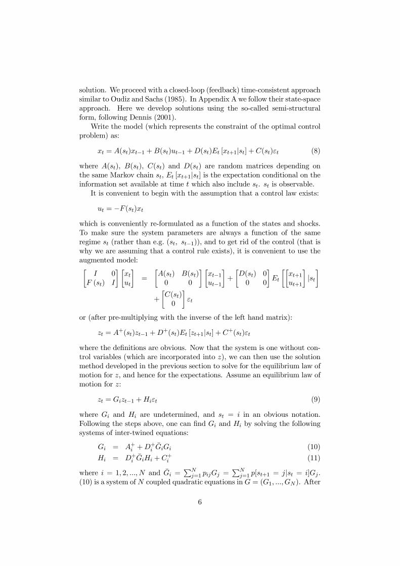
In this paper we conduct the following experiments. We assume that thereis a structural break in some key parameters, e.g. α. We assume there issome probability P of a permanent shift up or down. We then plot selectedresponse coefficients as a function of P .
In the graphs we plot a mixture of experiments. Firstly, we assume in atwo-state model that there is a probability p that there will be a change inthe coefficient, and a probability q that once it has changed regime it willswitch back. The Markov matrix is given by:
P =
·1− p pq 1− q
¸.
In the first set of experiments we assume that q = 0, that is once a switch hasoccurred there is no switch back. On the same graphs we plot a three-stateproblem using the Markov matrix:
P =
1− p 12p
12p
q 1− q 0q 0 1− q
where there is equal likelihood of two changes–which we choose to be upor down by the same amount–so we can get a handle on the certainty
14

0 0.2 0.4 0.6 0.8 10.96
0.98
1
1.02
1.04
1.06
1.08
1.1
1.12y
α=1α=.6symmetric
0 0.2 0.4 0.6 0.8 11.2
1.3
1.4
1.5
1.6
1.7
1.8
1.9
2π
0 0.2 0.4 0.6 0.8 10.48
0.485
0.49
0.495
0.5
0.505
0.51R(-1)
0 0.2 0.4 0.6 0.8 10.04
0.045
0.05
0.055
0.06
0.065q
0 0.2 0.4 0.6 0.8 1-0.056
-0.054
-0.052
-0.05
-0.048
-0.046
-0.044
-0.042q(-1)
0 0.2 0.4 0.6 0.8 1-0.17
-0.16
-0.15
-0.14
-0.13
-0.12k
Figure 1: Effect of changes in α
equivalence of the results. This is the red (usually central) line on thegraphs.
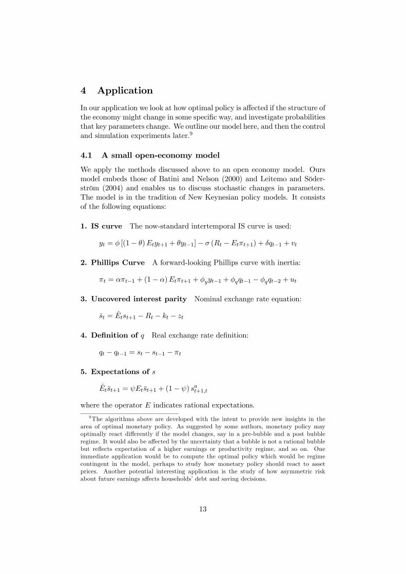
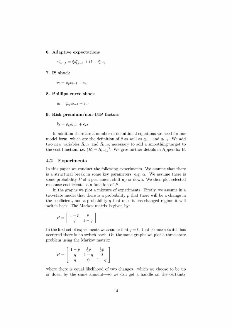
We begin by assuming that all changes are expected to be permanent(q = 0). In Figure 1 we show the effect of a change in α from the centralcase of 0.8. An anticipated fall requires a more aggressive response to theoutput gap for example, but only past some critical point. In Figure 2 weshow the same effect on σ. A similar pattern emerges, but with no markedswitching effect on the real exchange rate and output coefficients. Figure 3illustrates an almost perfect certainty equivalence result for changes to theexchange rate pass through coefficient, as the red line is near horizontal.
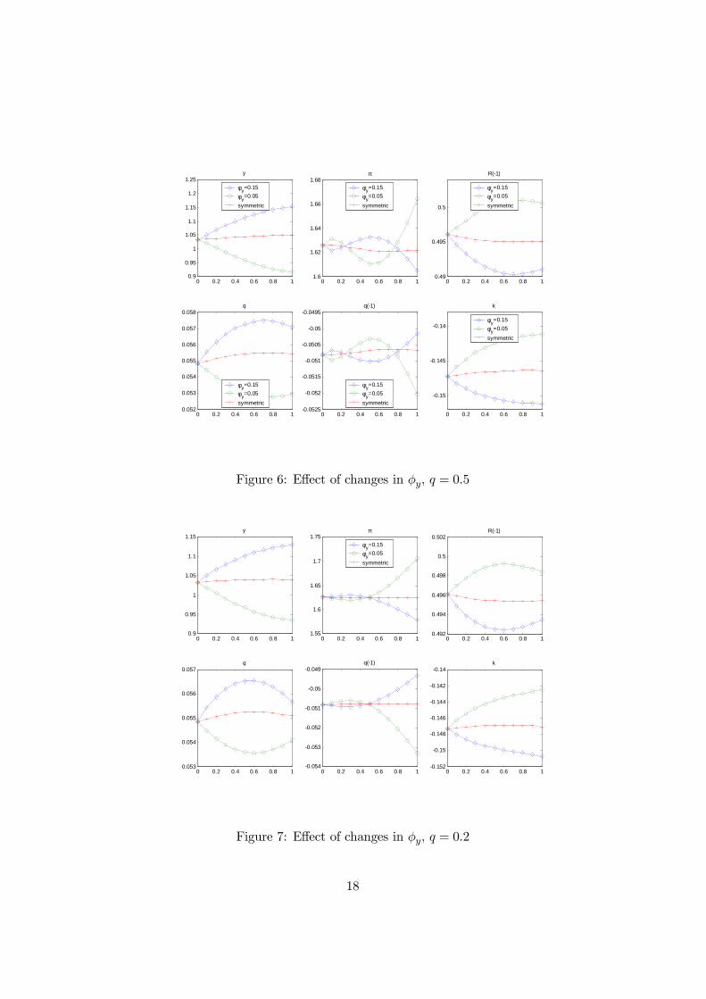
However if we consider changes to φy a different picture emerges (Figure4). Here complicated tradeoffs between coefficients occur. This seems par-ticularly true of the coefficients on the real exchange rate and the inflationrate. In Figure 5 changes to ϕ have small and predictable effects.
As φy seems an important parameter we plot this for different assump-tions about q. Figure 6 refers to the case q =0.5, and Figure 7 refers toq =0.25. The pattern of trade-offs in coefficients seems to be preserved.
15
0 0.2 0.4 0.6 0.8 10.98
1
1.02
1.04
1.06
1.08
1.1y
0 0.2 0.4 0.6 0.8 11.58
1.6
1.62
1.64
1.66π
0 0.2 0.4 0.6 0.8 10.46
0.48
0.5
0.52
0.54
0.56
0.58R(-1)
σ=.3σ=.1symmetric
0 0.2 0.4 0.6 0.8 10.051
0.052
0.053
0.054
0.055
0.056
0.057
0.058q
0 0.2 0.4 0.6 0.8 1-0.0515
-0.051
-0.0505
-0.05
-0.0495
-0.049q(-1)
0 0.2 0.4 0.6 0.8 1-0.18
-0.17
-0.16
-0.15
-0.14
-0.13
-0.12k
Figure 2: Effect of changes in σ
0 0.2 0.4 0.6 0.8 11.01
1.02
1.03
1.04
1.05
1.06
1.07y
φq=.035
φq=.015
symmetric
0 0.2 0.4 0.6 0.8 11.58
1.6
1.62
1.64
1.66
1.68
1.7π
0 0.2 0.4 0.6 0.8 10.4952
0.4954
0.4956
0.4958
0.496
0.4962
0.4964
0.4966
0.4968R(-1)
0 0.2 0.4 0.6 0.8 10.045
0.05
0.055
0.06
0.065
0.07q
0 0.2 0.4 0.6 0.8 1-0.07
-0.06
-0.05
-0.04
-0.03q(-1)
0 0.2 0.4 0.6 0.8 1-0.17
-0.16
-0.15
-0.14
-0.13
-0.12k
Figure 3: Effect of changes in φq
16

0 0.2 0.4 0.6 0.8 10.8
0.9
1
1.1
1.2y
0 0.2 0.4 0.6 0.8 1
1.6
1.7
1.8
1.9π
0 0.2 0.4 0.6 0.8 10.485
0.49
0.495
0.5
0.505
0.51
0.515R(-1)
φy=0.15
φy=0.05
symmetric
0 0.2 0.4 0.6 0.8 10.05
0.052
0.054
0.056
0.058
0.06
0.062q
0 0.2 0.4 0.6 0.8 1-0.058
-0.056
-0.054
-0.052
-0.05
-0.048
-0.046q(-1)
0 0.2 0.4 0.6 0.8 1-0.155
-0.15
-0.145
-0.14
-0.135k
Figure 4: Effect of a change in φy
0 0.2 0.4 0.6 0.8 10.92
0.94
0.96
0.98
1
1.02
1.04y
0 0.2 0.4 0.6 0.8 1
1.4
1.5
1.6
1.7π
0 0.2 0.4 0.6 0.8 10.48
0.485
0.49
0.495
0.5R(-1)
ψ=1ψ=0.5symmetric
0 0.2 0.4 0.6 0.8 10.0545
0.055
0.0555
0.056
0.0565
0.057
0.0575q
0 0.2 0.4 0.6 0.8 1-0.052
-0.05
-0.048
-0.046
-0.044
-0.042
-0.04q(-1)
0 0.2 0.4 0.6 0.8 1-0.2
-0.19
-0.18
-0.17
-0.16
-0.15
-0.14k
Figure 5: Effect of changes in ϕ
17
0 0.2 0.4 0.6 0.8 10.9
0.95
1
1.05
1.1
1.15
1.2
1.25y
φy=0.15
φy=0.05
symmetric
0 0.2 0.4 0.6 0.8 11.6
1.62
1.64
1.66
1.68π
φy=0.15
φy=0.05
symmetric
0 0.2 0.4 0.6 0.8 10.49
0.495
0.5
R(-1)
φy=0.15
φy=0.05
symmetric
0 0.2 0.4 0.6 0.8 10.052
0.053
0.054
0.055
0.056
0.057
0.058q
φy=0.15
φy=0.05
symmetric
0 0.2 0.4 0.6 0.8 1-0.0525
-0.052
-0.0515
-0.051
-0.0505
-0.05
-0.0495q(-1)
φy=0.15
φy=0.05
symmetric
0 0.2 0.4 0.6 0.8 1
-0.15
-0.145
-0.14
k
φy=0.15
φy=0.05
symmetric
Figure 6: Effect of changes in φy, q = 0.5
0 0.2 0.4 0.6 0.8 10.9
0.95
1
1.05
1.1
1.15y
0 0.2 0.4 0.6 0.8 11.55
1.6
1.65
1.7
1.75π
φy=0.15
φy=0.05
symmetric
0 0.2 0.4 0.6 0.8 10.492
0.494
0.496
0.498
0.5
0.502R(-1)
0 0.2 0.4 0.6 0.8 10.053
0.054
0.055
0.056
0.057q
0 0.2 0.4 0.6 0.8 1-0.054
-0.053
-0.052
-0.051
-0.05
-0.049q(-1)
0 0.2 0.4 0.6 0.8 1-0.152
-0.15
-0.148
-0.146
-0.144
-0.142
-0.14k
Figure 7: Effect of changes in φy, q = 0.2
18

5 Simulating the model under symmetric and asym-metric beliefs
The above indicates how we calculate optimal policies. It has built into itassumptions about agent and policymaker perceptions about each other’sbehaviour. Consider the following. Our control algorithm solves a fixedpoint problem, which can be succinctly represented as follows:
1. The policy maker (cb) computes policy u as a function of the proba-bility P and the private sector’s (ps) expectations Eps, that is:
ucb = u(P, Eps).
2. In turn, the private sector forms expectations Eps as a function of theprobability P and the policy rule ucb, that is:
Eps = E (P, ucb) .
3. Hence, ucb = u (P,Eps) = u (P,E (P, ucb)). The algorithm solves forthe fixed point ucb. It is assumed that P is the true probability gov-erning the transition across regimes.
These expectations are determined by the various agent’s perceived val-ues for P . All, some or none of these beliefs may be accurate. We cansimulate the model under a variety of assumptions about perceived valuesfor P .
5.1 A number of cases
Policy and expectations can be set under different assumptions than above.Assumptions regarding what each agent believes or knows about the world,the transition probabilities and the other agent’s decision problem. Thereare a number of cases that we consider, which are not exhaustive.
The first case we consider is one in which all agents share the same beliefsabout the probability matrix P (as well as everything else) but such beliefsmay be wrong. Let us indicate these beliefs with P . The problem can nowbe characterised by the pair of decision rules:
ucb = u(P , Eps)
Eps = E(P , ucb)
The problem is solved as before: ucb = u(P , Eps) = u³P , E (P, ucb)
´with
the difference being the different probability matrix P . Once ucb and Eps
have been found, they can be substituted out from the true model, obtain-ing a reduced form. This reduced form is the same as obtained under P .
19
However, it needs to be simulated under the true (but unknown to agents)value of P . One can compare responses under P and P to gauge the possi-ble errors involved in selecting P 6= P . If P is genuinely unknown, one cancompute the losses corresponding to the probability pairing
³P , P
´, where
P are the probabilities chosen by agents and P is the realisation of thetrue probability. The losses can inform the selection of as ‘optimal’ P thatminimises risk. For example, it can be selected using a min-max criterionor some other criterion. Operationally this requires that the policymakeris believed by all other agents in their assessment of the probability, so thepolicymaker can influence expectations through this channel. In this circum-stance the policymaker seeks to modify expectations to its advantage, thatof increased robustness. This can be seen as a way of manipulating agentsthat is akin to time inconsistency, but in effect as long as beliefs about thetrue probability never change then agents are never fooled and there is noincentive to renege.
The second case is one in which the private sector correctly perceivesP and perfectly knows the policy rule adopted by the policymaker. Thepolicymaker, on the other hand, has beliefs P , which in general differ fromthe true P , and also believes that the public shares those beliefs and henceforms expectations according to E
³P , ucb
´, i.e.:
ucb = u³P , E
³P , ucb
´´.
As the public correctly perceives P and the beliefs of the policymaker:
Eps = E (P, ucb) = E³P, u
³P , E
³P , ucb
´´´.
To find the equilibrium solution, one needs to find the fixed point in ucb =
u³P , E
³P , ucb
´´, which is done using the standard algorithm. Then ucb
is substituted out from the true model. The solution algorithm for forwardlooking models with regime shifts will contextually compute the expectationsEps = E(P, ucb) based on the true P as well as the policy ucb computed inthe previous step.
A third case is one in which the policymaker and the private sector donot share the same beliefs but perfectly understand each other’s beliefs anddecisions. Namely:
ucb = u(P , Eps)
Eps = E(P , ucb)
where in general P 6= P . Both P and P may also be different from the trueP . The standard algorithm needs to be modified to allow computation of thiscase. If an equilibrium exists, we can designate it the ‘known disagreement’
20
equilibrium. A special case of this is a variation of case two illustrated above:the policymaker chooses policy ucb = u
³P , Eps
´knowing that the public
has knowledge of the true probability matrix P , i.e. Eps = E (P, ucb).A fourth case is one in which a disagreement is unknown to both players:
ucb = u³P , E
³P , ucb
´´Eps = E
¡P , u
¡P , Eps
¢¢.
The standard algorithm can be run twice to solve for ucb and for Eps sepa-rately. Then, ucb and Eps need to be substituted out from the true modelto find the reduced form associated with this case.
There are, of course, many other cases which can be considered. Eachagent may form beliefs not only about the true model but also about theother agent’s beliefs about the true model, beliefs about his own beliefs,beliefs about his own beliefs over the other beliefs, and so on ad infinitum.This problem of infinite regress is not dealt with here. It is also clear thatthere could be considerable value to private information, as in Morris andShin (2002). We do not further consider the strategic advantages that mayaccrue here.
5.2 Learning
When simulating the model under the previous cases we implicitly assumethat agents do not learn through time. This is clearly not realistic butthere are two ways of defending the approach. First, the simulations help usinform about the choice of P , and therefore we are actually learning fromthem. Second, we could extend the algorithm to allow for passive learning.In other words, agents updates their probabilities using (for example) aBayesian scheme in every period, but they make decision assuming thatthese probabilities will not change in the future. This is in some waysrealistic: not all agents are so rational as to anticipate the way they willlearn in the future, i.e. know the law of motion of the probabilities. Inthis case of passive learning, Bayesian techniques can be used to updatethe probabilities period by period, and the above algorithm can be used tocompute the policymaker’s instrument choice as well as the private sector’sexpectations of future variables. A more sophisticated algorithm may recordthe evolution of the probabilities and estimate a law of motion for them.Thus the policymaker will need to solve a more sophisticated control problemin which he has to allow for future variation in the probabilities.
6 Simulation results
We plot a variety of responses in the following graphs.
21

0 2 4 6 8 10 12 140
0.2
0.4
0.6
0.8
1y
p=0Case 1: p=0.5Case 2: p=0.5Case 3: p=0.5
0 2 4 6 8 10 12 14-1.4
-1.2
-1
-0.8
-0.6
-0.4
-0.2
0π
p=0Case 1: p=0.5Case 2: p=0.5Case 3: p=0.5
0 2 4 6 8 10 12 14-0.5
0
0.5
1
1.5
2
2.5
3q
p=0Case 1: p=0.5Case 2: p=0.5Case 3: p=0.5
0 2 4 6 8 10 12 14-2
-1.5
-1
-0.5
0R
p=0Case 1: p=0.5Case 2: p=0.5Case 3: p=0.5
Figure 8: α goes from 0.8 to 0.6 with p = 0.5
• Case 1: both agents incorporate uncertainty as well as each otherreactions.
• Case 2: only the central bank factors in uncertainty while the privatesector does not and assumes regime 1 persists forever.
• Case 3: the central bank has a certainty equivalent rule, which isunderstood by the public, but the public factors in the probability ofa regime shift
In each of the graphs the blue line is the ‘certainty equivalent’ policy, sothat p = 0.
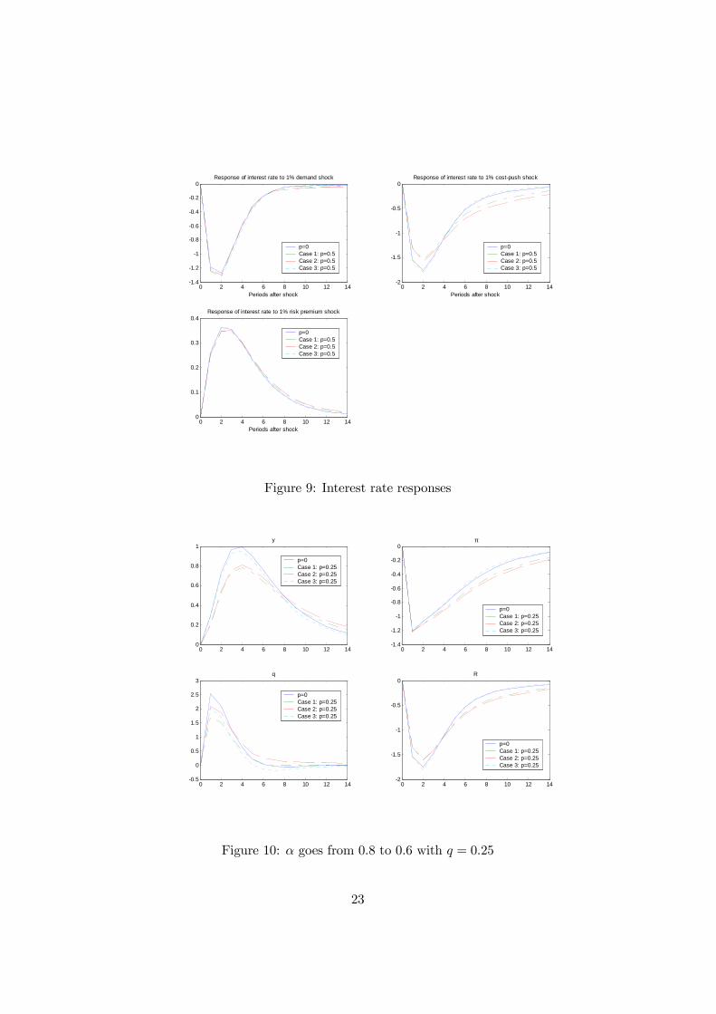
We concentrate on a break in α, as before possibly falling from 0.8 to0.6. In Figure 8 we show a supply shock of unity and the assumption thatp = 0.5. Here the responses of the output gap, inflation, the real exchangerate and interest rates are shown for each of the scenarios above. In Figure9 we show the interest rate responses for this and other shocks. In Figure10 we repeat the analysis for p = 0.25. It is clear that the perceptions ofthe various players can matter a great deal.
Now consider Figure 11. This simulation assumes break in α jumpingdown to 0.6 from 0.8. There is an initial negative inflationary shock and thenthe break in α occurs in period 3 (with probability 50% we would expectthe breaks to concentrate mostly in period 2 and 3). You can see that not
22
0 2 4 6 8 10 12 14-1.4
-1.2
-1
-0.8
-0.6
-0.4
-0.2
0
Periods after shock
Response of interest rate to 1% demand shock
p=0Case 1: p=0.5Case 2: p=0.5Case 3: p=0.5
0 2 4 6 8 10 12 14-2
-1.5
-1
-0.5
0
Periods after shock
Response of interest rate to 1% cost-push shock
p=0Case 1: p=0.5Case 2: p=0.5Case 3: p=0.5
0 2 4 6 8 10 12 140
0.1
0.2
0.3
0.4
Periods after shock
Response of interest rate to 1% risk premium shock
p=0Case 1: p=0.5Case 2: p=0.5Case 3: p=0.5
Figure 9: Interest rate responses
0 2 4 6 8 10 12 140
0.2
0.4
0.6
0.8
1y
p=0Case 1: p=0.25Case 2: p=0.25Case 3: p=0.25
0 2 4 6 8 10 12 14-1.4
-1.2
-1
-0.8
-0.6
-0.4
-0.2
0π
p=0Case 1: p=0.25Case 2: p=0.25Case 3: p=0.25
0 2 4 6 8 10 12 14-0.5
0
0.5
1
1.5
2
2.5
3q
p=0Case 1: p=0.25Case 2: p=0.25Case 3: p=0.25
0 2 4 6 8 10 12 14-2
-1.5
-1
-0.5
0R
p=0Case 1: p=0.25Case 2: p=0.25Case 3: p=0.25
Figure 10: α goes from 0.8 to 0.6 with q = 0.25
23

0 2 4 6 8 10 12 140
0.2
0.4
0.6
0.8
1y
p=0Case 1: p=0.5Case 2: p=0.5Case 3: p=0.5
0 2 4 6 8 10 12 14-1.4
-1.2
-1
-0.8
-0.6
-0.4
-0.2
0π
p=0Case 1: p=0.5Case 2: p=0.5Case 3: p=0.5
0 2 4 6 8 10 12 14-1
0
1
2
3q
p=0Case 1: p=0.5Case 2: p=0.5Case 3: p=0.5
0 2 4 6 8 10 12 14-2
-1.5
-1
-0.5
0
0.5R
p=0Case 1: p=0.5Case 2: p=0.5Case 3: p=0.5
Figure 11: Negative inflation shock, break to α in period 3, p = 0.5
taking into account uncertainty produces a somewhat ‘bumpier’ economy.Note that when the break occurs, in all cases the policymaker can observe thebreak and switches to the same policy rule. However, because the system isat that point in a different state following the different policies, the responsesfollow different paths from that point onwards, though all converging in thelong run towards equilibrium. In Figure 12 we reduce the probability to0.25. What does this imply? Policy should be loosened less in response toa negative shock but should then return more gradually to neutral stance.
7 Conclusions
In this paper we have investigated optimal time-consistent monetary policywhen the model is subject to regime shifts driven by Markov processes. Wehave barely scratched the surface of the control and simulation experimentsthat can be carried out. We in general find that policies are more cautiouswith this form of uncertainty. Recall that we are considering time consistentpolicies. If the monetary authorities are unable to affect expectations at allit may be that they would do almost nothing.
We have tried out a number of possible simulation scenarios. As themain source of uncertainty here is the Markov process and not the model(we know all the alternative models or parameterisations) and indeed howlikely we are to switch between them. It is an interesting problem to extend
24

0 2 4 6 8 10 12 140
0.2
0.4
0.6
0.8
1y
p=0Case 1: p=0.25Case 2: p=0.25Case 3: p=0.25
0 2 4 6 8 10 12 14-1.4
-1.2
-1
-0.8
-0.6
-0.4
-0.2
0π
p=0Case 1: p=0.25Case 2: p=0.25Case 3: p=0.25
0 2 4 6 8 10 12 14-0.5
0
0.5
1
1.5
2
2.5
3q
p=0Case 1: p=0.25Case 2: p=0.25Case 3: p=0.25
0 2 4 6 8 10 12 14-2
-1.5
-1
-0.5
0
0.5R
p=0Case 1: p=0.25Case 2: p=0.25Case 3: p=0.25
Figure 12: Negative inflation shock, break to α in period 3, p = 0.25
this model to where we are uncertain about the Markov process and modelthe learning over that rather than behavioural parameters directly.
References
Aoki, M. (1967). Optimization of Stochastic Systems. New York: AcademicPress.
Basar, T. and G. J. Olsder (1999). Dynamic Noncooperative Game Theory(second ed.), Volume 23 of Classics in Applied Mathematics. Philadelphia:SIAM.
Batini, N. and E. Nelson (2000). When the bubble bursts: Mone-tary policy rules and foreign exchange market behavior. Available athttp://research.stlouisfed.org/econ/nelson/bubble.pdf.
Blake, A. P. (2004). Analytic derivative in linear rational expectations mod-els. Computational Economics 24 (1), 77—96.
Blanchard, O. and C. Kahn (1980). The solution of linear difference modelsunder rational expectations. Econometrica 48, 1305—1311.
Costa, O. L. V., M. D. Fragoso, and R. P. Marques (2005). Discrete-TimeMarkov Jump Linear Systems. Probability and its Applications. Springer-Verlag.
25

Dennis, R. (2001). Optimal policy in rational-expectations models: Newsolution algorithms. Working Papers in Applied Economic Theory 2001-09, Federal Reserve Bank of San Francisco.
Dennis, R. and U. Söderström (2002). How important is precommitment formonetary policy? Working paper, Sveriges Riksbank.
Fershtman, C. (1989). Fixed rules and decision rules: Time consistency andsubgame perfection. Economics Letters 30 (3), 191—194.
Hamilton, J. D. (1994). Time Series Analysis. Princeton, NJ: PrincetonUniversity Press.
Kozicki, S. (2004). How do data revisions affect the evaluation and conductof monetary policy? Federal Reserve Bank of Kansas City EconomicReview 89 (1), 5—38.
Leitemo, K. and U. Söderström (2004). Simple monetary policy rulesand exchange rate uncertainty. Journal of International Money and Fi-nance 24 (3), 481—507.
Ljungqvist, L. and T. J. Sargent (2000). Recursive Macroeconomic Theory.Cambridge, MA: The MIT Press.
Morris, S. and H. S. Shin (2002). Social value of public information. Amer-ican Economic Review 92, 1521—1534.
Oudiz, G. and J. Sachs (1985). International policy coordination in dynamicmacroeconomic models. In W. H. Buiter and R. C. Marston (Eds.), In-ternational Economic Policy Coordination. Cambridge: Cambridge Uni-versity Press.
Planas, C. and A. Rossi (2004). Can inflation data improve the real-time re-liability of output gap estimates? Journal of Applied Econometrics 19 (1),121—33.
Roberds, W. (1987). Models of policy under stochastic replanning. Inter-national Economic Review 28 (3), 731—755.
Swanson, E. T. (2004). Signal extraction and non-certainty-equivalence inoptimal monetary policy rules. Macroeconomic Dynamics 8 (1), 27—50.
Zampolli, F. (2005). Optimal monetary policy in a regime-switching econ-omy. Discussion paper, Bank of England.
26
A State space solutions
In this Appendix we detail an alternative method for the calculation of ex-plicitly time consistent policies. In the next section we consider the rationalexpectations solution, perhaps conditional on a given policy rule. We thenconsider the dynamic programming solution as a generalisation of the Oudizand Sachs (1985) procedure. As the problem is certainty equivalent we onlydiscuss the deterministic case.
A.1 A generalised rational expectations solution
Define a rational expectations model in state space as:·zt+1
E [xt+1|It]¸=
·Ai11 Ai
12
Ai21 Ai
22
¸·ztxt
¸. (24)
We seek a solution of the form:
xt = −N izt (25)
where we recognise that there may be a change in regime of some sort. Fortwo possible regimes this means thatE [xt+1|It] = −(pi1N1+pi2N2)E [zt+1|It]for a model in ‘state i’ or, more generally, for l possible regimes:
E [xt+1|It] = − lX
j=1
pijNj
E [zt+1|It] (26)
for the ith regime. Using this in the model (24) gives:
− lX
j=1
pijNj
¡Ai11zt +Ai
12xt¢= Ai
21zt +Ai22xt (27)
implying:
− lX
j=1
pijNj
Ai12 +Ai
22
xt
=
lXj=1
pijNj
Ai11 +Ai
21
zt (28)
or:
xt = −³N iAi
12 +Ai22
´−1 ³N iAi
11 +Ai21
´zt
= −N izt.
27

where N i =Pl
j=1 pijNj . We can develop an iteration based on this as:
N1k+1 =
lXi=1
p1iNik+1
N1k =
³N1k+1A
112 +A122
´−1 ³N1k+1A
111 +A121
´N2k+1 =
lXi=1
p2iNik+1
N2k =
³N2k+1A
212 +A222
´−1 ³N2k+1A
211 +A221
´...
N lk+1 =
lXi=1
pliNik+1
N lk =
³N lk+1A
l12 +Al
22
´−1 ³N lk+1A
l11 +Al
21
´which continues until convergence. Thus in equilibrium for the ith regimewe get:
− lX
j=1
pijNj
¡Ai11 −Ai
12Ni¢=¡Ai21 −Ai
22Ni¢
(29)
as the solution to the ith linked Riccati-type equation.10
A number of remarks should be made. First, in common with Oudizand Sachs (1985) we assume that
³N ik+1A
i12 +Ai
22
´is non-singular. This is
almost always the case in our experience. Secondly, if the model is instead:·Ei11 Ei
12
Ei21 Ei
22
¸·zt+1
E [xt+1|It]¸=
·Ai11 Ai
12
Ai21 Ai
22
¸·ztxt
¸(30)
we can develop an equivalent iteration assuming that Ei11 and Ai
22 are non-singular. Indeed, the semi-structural form model can be written:·
I 00 Bi
¸·xt
E [xt+1|It]¸=
·0 I−Ai I
¸·xt−1xt
¸(31)
which conforms to those restrictions. Finally, if the regimes are all the samethen the solution reduces down to:
−N (A11 −A12N) = (A21 −A22N) (32)
which could be solved using the method of Blanchard and Kahn (1980) oriteratively as above.10See Blake (2004) for a discussion of the types of Riccati equations used in rational
expectations solutions.
28

A.2 Control
Let the control model in state space be:·zt+1
E [xt+1|It]¸=
·Ai11 Ai
12
Ai21 Ai
22
¸·ztxt
¸+
·Bi1
Bi2
¸ut. (33)
We can apply the solutions of the previous section to yield:
xt = −³N iAi
12 +Ai22
´−1 ³N iAi
11 +Ai21
´zt
−³N iAi
12 +Ai22
´−1 ³N iBi
1 +Bi2
´ut
= −J izt −Kiut. (34)
For a given feedback rule, say ut = −F izt, then:
xt = −(J i −KiF i)zt
= −N izt. (35)
Now consider the discounted quadratic objective function:
Ct =1
2
∞Xt=0
βt¡z0tQzt + u0tRut
¢. (36)
More generally we would consider a cost function of the form:
Ct = s0tQst + 2u0tUst + u0tRut (37)
where st =·ztxt
¸and we assign costs to the jump variables and covariances.
We use (36) to reduce the amount of algebra without changing the essentialmessage. Algebra for the complete cost case is available on request. (36)is minimised subject to (33) and a time consistency restriction. We nextsketch a solution in the standard case and then for the Markov switchingcase.
A.2.1 Standard time consistent policies
The ‘standard’ Oudiz and Sachs (1985) dynamic programming solution isobtained from the following. Write the value function as:
Vt =1
2z0tStzt = minut
1
2
¡z0tQzt + u0tRut
¢+
β
2z0t+1St+1zt+1. (38)
Note that the first line of the model is:
zt+1 = A11zt +A12xt +B1ut (39)
29

which we substitute in as the constraint. We can obtain the following deriv-atives:
∂Vt∂ut
= Rut + βB01St+1zt+1 (40)
∂Vt∂xt
= βA012St+1zt+1 (41)
∂xt∂ut
= −K (42)
with the last obtained from (34), our time consistency restriction. Thisreflects intra-period leadership with respect to private agents, so can beseen as reflecting Stackelberg behaviour. Using (34) we can also write (39)as:
zt+1 = (A11 −A12J)zt + (B1 −A12K)ut. (43)
We can use (40)—(42) and (43) to obtain the first order condition:
∂Vt∂ut
+∂Vt∂xt
∂xt∂ut
=¡R+ β(B01 −K0A012)St+1(B1 −A12K)
¢ut
+β(B01 −K0A012)St+1(A11 −A12J)zt
= 0
⇒ ut = −β ¡R+ β(B01 −K0A012)St+1(B1 −A12K)¢−1
× ¡(B01 −K0A012)St+1(A11 −A12J)¢zt
= −FSzt (44)
with the subscript emphasising the Stackelberg equilibrium. The value func-tion can be written:
z0tStzt = z0t¡Q+ F 0SRFS + β(A011 − J 0A012 − F 0S(B
01 −K0A012))
×St+1(A11 −A12J − (B1 −A12K)FS)) zt
implying:
St = Q+F 0SRFS+β(A011−N 0A012−F 0SB01)St+1(A11−A12N−B1FS) (45)where N = J −KFS.
Note we could assume that ∂xt/∂ut = 0, the Nash assumption, andinstead obtain:
∂Vt∂ut
=¡R+ βB01St+1(B1 −A12K)
¢ut
+βB01St+1(A11 −A12J)zt = 0
⇒ ut = −β ¡R+ βB01St+1(B1 −A12K)¢−1
× ¡B01St+1(A11 −A12J)¢zt
= −FNzt (46)
30

with associated Riccati equation:
St = Q+F 0NRFN +β(A011−N 0A012−F 0NB01)St+1(A11−A12N −B1FN)
with N = J−KFN now. This gives us a second time consistent equilibriumto investigate.
A.2.2 Markov switching models
We now turn to the case with random matrices. We modify the value func-tion for the ith regime to:
V it = minut
1
2
¡z0tQzt + u0tRut
¢+ βEtV
it+1 (47)
where we need to make some assumption about V it+1. In common with what
went before we will weight the forward value function by the probabilitythat it comes to pass. However, the information set assumed will determinethe exact form.
In either case the required modification is very simple, and it is easyto see that one possibility is to replace the last term with the probabilityweighted values of the alternative future value functions to give:
1
2z0tS
itzt = minut
1
2
¡z0tQzt + u0tRut
¢+
β
2zi0t+1S
it+1z
it+1. (48)
where:
zit+1 = (Ai11 −Ai
12Ji)zt + (B
i1 −Ai
12Ki)ut
and Xi =Pl
j=1 pijXj for any X, the same as the weight scheme we had
before for the expectations generating mechanism. In so doing we are as-suming that the policymaker identifies the regime that they currently facebut is uncertain about any future one. If uncertainty extended to the currentregime, then the optimisation problem would be:
1
2z0tS
itzt = minut
1
2
¡z0tQzt + u0tRut
¢+
β
2z0t+1S
it+1zt+1 (49)
where:
zt+1 = (Ai11 − Ai
12J)zt + (Bi1 − Ai
12K)ut
as policymakers would only know the previous policy regime, i, and thetransition probabilities from that regime and so must ‘average’ the modelsto give the anticipated state.
What do all other agents expect? The equilibrium policy is one whereagents expectations of the future policy is consistent with the assumed prob-abilities. Thus the value of (35) calculated to determine expectations is (in
31

equilibrium) consistent with the policy actually followed, although we canmodify this by having differing perceived probabilities across the policy-maker and other agents. In fact, it is only across probabilities that we allowagents to differ in what they expect. Note that when this happens thereis no intrinsic time inconsistency, as we discuss above, but rather this maylead to an inferior (or possibly superior) outcome. One of the advantages tothe semi-structural form of the main text is that this is much more easilyseen due to the fixed point nature of the solution.
Given expectations we need to determine that policy. For the first, Stack-elberg, case, the first order condition then yields:
∂V it
∂ut+
∂V it
∂xt
∂xt∂ut
=³R+ β(Bi0
1 −Ki0Ai012)S
it+1(B
i1 −Ai
12Ki)´ut
+β(Bi01 −Ki0Ai0
12)Sit+1(A
i11 −Ai
12Ji)zt = 0
⇒ ut = −β³R+ β(Bi0
1 −Ki0Ai012)S
it+1(B
i1 −Ai
12Ki)´−1
׳(Bi0
1 −Ki0Ai012)S
it+1(A
i11 −Ai
12Ji)´zt
= −F iSzt.
Substituting into the value function we have the following Ricatti-type equa-tion for regime i:
Sit = Q+F i0
SRFiS +β(Ai0
11−N i0Ai012−F i0
SBi01 )S
it+1(A
i11−Ai
12Ni−Bi
1FiS)
where N i = J i −KiF iS.
In the second case, we get the Stackelberg solution:
∂V it
∂ut+
∂V it
∂xt
∂xt∂ut
=³R+ β(Bi0
1 −Ki0Ai012)S
it+1(B
i1 − Ai
12Ki)´ut
+β(Bi01 −Ki0Ai0
12)Sit+1(A
i11 − Ai
12Ji)zt = 0
⇒ ut = −β³R+ β(Bi0
1 −Ki0Ai012)S
it+1(B
i1 − Ai
12Ki)´−1
׳(Bi0
1 −Ki0Ai012)S
it+1(A
i11 − Ai
12Ji)´zt
= −F iSzt
with:
Sit = Q+F i0
SRFiS+β(Ai0
11−N i0Ai012−F i0
SBi01 )S
it+1(A
i11−Ai
12Ni−Bi
1FiS).
There is an open question as to which solution should be used. TheStackelberg case is almost always used (our semi-structural form admits noother). However, it implies a degree of leadership over the private sector,which we could interpret as commitment. This may be appropriate for somepolicymakers, but may be questionable for the monetary authority. It is anempirical question as to wheter there is value to such commitments.
32

A.3 Iterative schemes
Consider the Stackelberg equilibrium with current state information forevery participant. A possible solution scheme is shown in Table 1. Wecan develop Nash solutions by deleting the relevant part of the policy rules.The resulting modified algorithm in Table 2.
The ‘no current information for the policymaker’ solutions involve prob-ability averaging the matrices A11, A12 and B1 in the recursions for F andS. The resulting algorithms are given in Tables 3 and 4. Note that thisinvolves different data sets for agents and policymakers, emphasised by thelack of the tilde’s over the system matrices in the equations determining Jand K.
We need to note the termination rules that we should observe. In thetables we merely terminate when the period count reaches 0. We wouldnormally terminate iteration before this if the matrices have converged toa steady state. In general, without the stochastic matrices, we would stopwhen abs(max(Nt+1−Nt)) < and abs(max(St+1−St)) < for some small. This does not work for the stochastic matrix case, as the future values arealways probability weighted, so we need to store N and S between iterationsseparately.
33

Table 1: FBS
SiT = S, N i
T = N , for i = 1, ..., l.for t = T − 1, 0for i = 1, l
N it+1 =
Plj=1pijN
jt+1
Sit+1 =
Plj=1pijS
jt+1
J i =³N it+1A
i12 +Ai
22
´−1 ³N it+1A
i11 +Ai
21
´Ki =
³N it+1A
i12 +Ai
22
´−1 ³N it+1B
i1 +Bi
2
´F iS = β
³R+ β(Bi0
1 −Ki0Ai012)S
it+1(B
i1 −Ai
12Ki)´−1
׳(Bi0
1 −Ki0Ai012)S
it+1(A
i11 −Ai
12Ji)´
N it = J i −KiF i
S
Sit = Q+ F i0
SRFiS + β(Ai0
11 −N i0t A
i012 − F i0
SBi01 )
×Sit+1(A
i11 −Ai
12Nit −Bi
1FiS)
endforendfor
34

Table 2: FBN
SiT = S, N i
T = N , for i = 1, ..., l.for t = T − 1, 0for i = 1, l
N it+1 =
Plj=1pijN
jt+1
Sit+1 =
Plj=1pijS
jt+1
J i =³N it+1A
i12 +Ai
22
´−1 ³N it+1A
i11 +Ai
21
´Ki =
³N it+1A
i12 +Ai
22
´−1 ³N it+1B
i1 +Bi
2
´F iN = β
³R+ βBi0
1 Sit+1(B
i1 −Ai
12Ki)´−1
Bi01 S
it+1(A
i11 −Ai
12Ji)
N it = J i −KiF i
N
Sit = Q+ F i0
NRFiN + β(Ai0
11 −N i0t A
i012 − F i0
NBi01 )
×Sit+1(A
i11 −Ai
12Nit −Bi
1FiN)
endforendfor
35

Table 3: FBS, policy information lag
SiT = S, N i
T = N , Ai11 =
Plj=1 pijA
j11, A
i12 =
Plj=1 pijA
j12
and Bi1 =
Plj=1 pijB
j1 for i = 1, ..., l.
for t = T − 1, 0for i = 1, l
N it+1 =
Plj=1pijN
jt+1
Sit+1 =
Plj=1pijS
jt+1
J i =³N it+1A
i12 +Ai
22
´−1 ³N it+1A
i11 +Ai
21
´Ki =
³N it+1A
i12 +Ai
22
´−1 ³N it+1B
i1 +Bi
2
´F iS = β
³R+ β(Bi0
1 −Ki0Ai012)S
it+1(B
i1 − Ai
12Ki)´−1
׳(Bi0
1 −Ki0Ai012)S
it+1(A
i11 − Ai
12Ji)´
N it = J i −KiF i
S
Sit = Q+ F i0
SRFiS + β(Ai0
11 −N i0t A
i012 − F i0
S Bi01 )
×Sit+1(A
i11 − Ai
12Nit − Bi
1FiS)
endforendfor
36

Table 4: FBN, policy information lag
SiT = S, N i
T = N , Ai11 =
Plj=1 pijA
j11, A
i12 =
Plj=1 pijA
j12 and Bi
1 =Plj=1 pijB
j1 for i = 1, ..., l.
for t = T − 1, 0for i = 1, l
N it+1 =
Plj=1pijN
jt+1
Sit+1 =
Plj=1pijS
jt+1
J i =³N it+1A
i12 +Ai
22
´−1 ³N it+1A
i11 +Ai
21
´Ki =
³N it+1A
i12 +Ai
22
´−1 ³N it+1B
i1 +Bi
2
´F iS = β
³R+ βBi0
1 Sit+1(B
i1 − Ai
12Ki)´−1
Bi01 S
it+1(A
i11 − Ai
12Ji)
N it = J i −KiF i
S
Sit = Q+ F i0
SRFiS + β(Ai0
11 −N i0t A
i012 − F i0
S Bi01 )
×Sit+1(A
i11 − Ai
12Nit − Bi
1FiS)
endforendfor
37

B Model in semi-structural form
The model can be written:
Hxt = Axt−1 +But−1 +DEt[xt+1|It] +Cεt
where the x, u and ε vectors are defined as:xt
1 yt2 πt3 st4 qt5 Etst+1 or Etst+16 sat+1,t7 vt8 ut9 kt10 qt11 qt−112 qt−113 qt−214 Rt−115 Rt−216 c17 zt18 bt19 st
ut
1 Rt
εt
1 evt2 eut3 ekt4 ezt
The parameters, similar to Batini and Nelson (2000) and Leitemo and Söder-ström (2004), were set as φ = 0.9, θ = 0.7, σ = 0.2, δ = 0.05, α = 0.8,φy = 0.1, φq = 0.025, ψ = 1 (full rationality unless stated otherwise; in ex-amining learning we set the updating parameter to ξ = 0.1), ρv = 0, ρu = 0and ρk = 0.753 consistent with a small open economy. The shock varianceswere set as σv = 1%, σu = 0.5%, and σk = 0.92%.
Finally, the policymaker’s preferences were set (in the main case) to beβ = 1, λy = 1, λπ = 2 and λ∆R = 0.1.
B.1 Loss function
Period function:
x0tRxt + u0tQut + 2x0tWut
38

R =
λy 0 0 · · · 00 λπ 0 · · · 00 0 0 · · · 0...
....... . .
...0 0 0 · · · 0
,Q = [λ∆R] ,
W =
0...0
−λ∆R
0
This implies that 2x0tWut = 2 (−Rt−1λ∆R)Rt = −2λ∆RRtRt−1.
39