Improving Markov Switching Models using Realized

Variance∗

Jia Liu † John M. Maheu ‡

This draft June 2017

Abstract

This paper proposes a class of models that jointly model returns and ex-post variance

measures under a Markov switching framework. Both univariate and multivariate re-

turn versions of the model are introduced. Estimation can be conducted under a fixed

dimension state space or an infinite one. The proposed models can be seen as nonlinear

common factor models subject to Markov switching and are able to exploit the infor-

mation content in both returns and ex-post volatility measures. Applications to equity

returns compare the proposed models to existing alternatives. The empirical results

show that the joint models improve density forecasts for returns and point predictions

of return variance. Using the information in ex-post volatility measures can increase

the precision of parameter estimates, sharpen the inference on the latent state variable

and improve portfolio decisions.

Keywords: Infinite hidden Markov model, Realized covariance, Density forecast, MCMC,

Portfolio choice

∗We thank the editor Andrew Patton and two anonymous referees for many helpful comments thatresulted in a significant revision of the paper. We thank Qiao Yang and seminar participants at the CEAannual meetings 2015, CESG 2015 and MEG 2015 for comments. Maheu is grateful to the SSHRC (grant435-2014-2015) for financial support.†DeGroote School of Business, McMaster University, Canada, liuj46@mcmaster.ca‡DeGroote School of Business, McMaster University, Canada and RCEA, Italy, maheujm@mcmaster.ca

1

1 Introduction

This paper proposes a new way of jointly modelling return and ex-post volatility measures

under a Markov switching framework. Parametric and nonparametric versions of the models

are introduced in both univariate and multivariate settings. The models are able to exploit

the information content in both return and ex-post volatility series. Compared to existing

models, the joint models improve density forecasts of returns, point predictions of realized

variance and portfolio decisions.

Since the pioneering work by Hamilton (1989) the Markov switching model has became

one of the standard econometric tools in studying various financial and economic data series.

The basic model postulates a discrete latent variable governed by a first-order Markov chain

that directs an observable data series. This modelling approach has been fruitfully employed

in many applications. For instance, Markov switching models have been used to identify bull

and bear markets in aggregate stock returns (Maheu and McCurdy, 2000; Lunde and Tim-

mermann, 2004; Guidolin and Timmermann, 2006; Maheu et al., 2012), to capture the risk

and return relationship (Pastor and Stambaugh, 2001; Kim et al., 2004), for portfolio choice

(Guidolin and Timmermann, 2008), for interest rates (Ang and Bekaert, 2002; Guidolin and

Timmermann, 2009) and foreign exchange rates (Engel and Hamilton, 1990; Dueker and

Neely, 2007). Recent work has extended the Markov switching model to an infinite dimen-

sion. The infinite hidden Markov model (IHMM), which is a Bayesian nonparametric model,

allows for a very flexible conditional distribution that can change over time. Applications of

IHMM include Jochmann (2015), Dufays (2016), Song (2014), Carpantier and Dufays (2014)

and Maheu and Yang (2016).

Realized variance (RV), constructed from intraperiod returns, is an accurate measure

of ex-post volatility. Andersen et al. (2001) and Barndorff-Nielsen and Shephard (2002)

formalized the idea of using higher frequency data to measure the volatility of lower frequency

data and show RV is a consistent estimate of quadratic variation under ideal conditions.

Barndorff-Nielsen and Shephard (2004b) generalized the idea of RV and introduced a set of

variance estimators called realized power variations. Furthermore, RV has been extended to

realized covariance (RCOV), which is an ex-post nonparametric measure of the covariance

of multivariate returns, by Barndorff-Nielsen and Shephard (2004a). A survey of RV and

related volatility proxies is Andersen and Benzoni (2009).

This paper is the first to exploit the information content of ex-post volatility measures in

a Markov switching context to improve estimation, forecasting and portfolio decisions.1 This

1Other papers that have used high frequency data to improve estimation and forecasting include Alizadehet al. (2002), Blair et al. (2001), Shephard and Sheppard (2010), Noureldin et al. (2012), Hansen et al. (2012)Hansen et al. (2014), Jin and Maheu (2013, 2016) and Maheu and McCurdy (2011).

2

is done for finite and infinite state models. We assume that regime changes in returns and

realized variance are directed by one common unobserved state variable. Closely related to

our approach is Takahashi et al. (2009) who propose a stochastic volatility model in which

unobserved log-volatility affects both RV and the variance of returns. They find improved

fixed parameter and latent volatility estimates but do not investigate forecast performance

or portfolio choice.

There is no reason to confine attention to RV, and therefore we investigate the use of other

volatility measures and in the multivariate setting realized covariance. Four versions of the

univariate return models are proposed. We consider RV, log(RV), realized absolute variation

(RAV), or log(RAV) as ex-post volatility measures coupled with returns to construct joint

models. We then extend the MS-RV specification to its multivariate version with RCOV.

It is more flexible to drop the finite state assumption and let the data determine the

number of states needed to fit the data. Using Bayesian nonparametric techniques, we

extend the finite state joint MS models to nonparametric versions. These models allow

the conditional distribution to change more flexibly and accommodate any nonparametric

relationship between returns and ex-post volatility.

Markov switching models have been particularly useful at monthly and quarterly fre-

quencies as the Markov chain dynamics are a dominate feature of the data.2 Therefore,

the proposed joint MS and joint IHMM models are compared to existing models in empir-

ical applications to monthly U.S. stock market returns including forecasting and portfolio

applications.

Based on the log-predictive Bayes factors, the proposed joint models strongly dominate

the models that only use returns. Moreover, we find the gains from joint modelling are

particularly large during high volatility episodes. The empirical results also show that the

joint models reduce the error in predicting realized variance. With the help of additional

information offered by RV, RAV and RCOV, posterior density intervals for parameters are

tighter and the inference on the unobservable state variables is improved. In general, adding

RV to a model improves the forecast performance of any MS model, finite or infinite, but

the best performing models are the joint infinite hidden Markov models.

Exploiting measures of ex-post volatility also lead to better portfolio choice outcomes.

Several portfolio exercises that use the models are considered over two sample periods. A

robust result is larger Sharpe ratios for models that incorporate realized variance or realized

covariance. In addition, investors are always willing to pay a positive performance fee to

obtain forecasts from these models for their investment decisions.

2Our models could be applied to higher frequency data but in this case additional structure would beneeded to capture the strong persistence in high frequency volatility Ryden et al. (1998).

3

This paper is organized as follows. In Section 2, we show how to incorporate ex-post

measures of volatility into Markov switching models. The joint MS models are extended to

the nonparametric versions in Section 3. Benchmark models used for comparison are found

in Section 4. Section 5 illustrates the Bayesian estimation steps and model comparison. A

univariate return application to the market index is found in Section 6 while a multivariate

return application to equity follows in Section 7. The next section concludes followed by an

appendix that gives detailed steps of posterior simulation.

2 Joint Markov Switching Models

In this section, we will focus on simple specifications of the conditional mean but dynamic

models with lags of the dependent variables could be used. We will first discuss the four

versions of univariate return joint models, then introduce the multivariate version.

Higher frequency data is used to construct ex-post volatility measures. Let rt,i denote

the ith intraperiod continuously compounded return in period t, i = 1, . . . , nt, where nt is

the number of intraperiod returns. Then the return and realized variance from t− 1 to t is

rt =nt∑i=1

rt,i, (1)

RVt =nt∑i=1

r2t,i. (2)

Andersen et al. (2001) and Barndorff-Nielsen and Shephard (2002) formalized the idea of

using higher frequency data to measure the volatility of rt. They show that RVt is a consistent

estimate of quadratic variation under ideal conditions.3 Similarly, for multivariate returns

Rt,i is the ith intraperiod d×1 return vector at time t and the time t return is Rt =∑nt

i=1Rt,i.

RCOVt denotes the associated realized covariance (RCOV) matrix which is computed as

follows,

RCOVt =nt∑i=1

Rt,iR′

t,i. (3)

3We have not made adjustments for market microstructure dynamics since our high-frequency data con-sists of daily returns and are relatively clean. Nevertheless, any of the existing approaches that correct formicrostructure dynamics in computing ex-post volatility measures could be used.

4

2.1 MS-RV Model

We first use RV as the proxy for ex-post volatility to build a joint MS-RV model. The

proposed K-state MS-RV model is given as follows.

rt∣∣st ∼ N(µst , σ

2st), (4)

RVt∣∣st ∼ IG(ν + 1, νσ2

st), (5)

Pi,j = p(st+1 = j|st = i), (6)

where st ∈ {1, . . . , K}. Conditional on state st, RVt is assumed to follow an inverse-gamma

distribution4 IG(ν + 1, νσ2st), where ν + 1 is the shape parameter and νσ2

st is the scale

parameter.

The basic assumption of this model is that RVt is subject to the same regime changes

as rt and share the same parameter σ2st .

5 Note, that RVt and the other volatility measures

used in this paper, are assumed to be a noisy measure of the state dependent variance σ2st .

Conditional on the latent state, the mean and variance of RVt are

E(RVt|st) =νσ2

st

(ν + 1)− 1= σ2

st , (7)

Var(RVt|st) =(σ2

st)2

(ν − 1). (8)

Therefore RVt is centered around σ2st , but in general, not equal to it. The variance of the

distribution of RVt is positively correlated with the realized variance itself. During high

volatility periods, the movements of realized variances are more volatile. Both the return

process and realized variance process are governed by the same underlying Markov chain

with transition matrix P .

Since σ2st influences both the return process and RVt process, the model can be seen as a

nonlinear common factor model.6 Exploiting the information content of RVt for σ2st can lead

to more precise estimates of model parameters, state variables and forecasts.

4If x ∼ IG(α, β), α > 0, β > 0 then it has density function:

g(x∣∣α, β) =

βα

Γ(α)x−α−1 exp

(−βx

).

The mean of x is E(x) = βα−1 for α > 1 and Var(x) = β2

(α−1)2(α−2) for α > 2.5Formally, the high frequency data generating process is assumed to be rt,i = µst/nt + (σst/

√nt)zt,i,

with zt,i ∼ NID(0, 1). Then E[∑nt

i=1 r2t,i

∣∣st] = µ2st/nt + σ2

st ≈ σ2st when the term µ2

st/nt is small due to ntbeing large.

6This is in contrast to linear dynamic factor models such as Forni and Reichlin (1998), Kose et al. (2003)and Stock and Watson (2010).

5

2.2 MS-logRV Model

Another possibility is to model the logarithm of RV as normally distributed. The MS-logRV

model is shown as follows,

rt∣∣st ∼ N (µst , exp(ζst)) , (9)

log(RVt)∣∣st ∼ N

(ζst −

1

2δ2st , δ

2st

), (10)

Pi,j = p(st+1 = j|st = i), (11)

where st ∈ {1, . . . , K}. In this model there are three state-dependent parameters: µst , ζst

and δ2st , which enable both the mean and variance of returns and log(RVt) to be state-

dependent. ζst − 12δ2st is the mean of log(RVt) and exp(ζst) is the variance of returns. Since

RVt is log-normal, E[RVt|st] = exp(ζst) which is assumed to be the variance of returns.

2.3 MS-RAV Model

Now we consider using realized absolute variation (RAV), instead of RV in the joint MS

model. Calculated using the absolute values of intraperiod returns, RAV is robust to jumps

and may be less sensitive to outliers Barndorff-Nielsen and Shephard (2004b). RAVt is

computed using intraperiod returns as

RAVt =

√π

2

√1

nt

nt∑i=1

|rt,i|, (12)

where rt,i denotes the ith intraperiod log-return in period t, i = 1, . . . , nt. It can be shown

that RAVt provides an estimate of the standard deviation of rt.7

Consistent with the inverse-gamma distribution to model the variance or its proxy, we as-

sume RAV follows a square-root inverse-gamma distribution (sqrt-IG). The density function

of sqrt-IG(α, β) is given by

f(x) =2βα

Γ(α)x−2α−1 exp

(− β

x2

), x > 0, α > 0, β > 0, (13)

7As before, if rt,i = µst/nt + (σst/√nt)zt,i, with zt,i ∼ NID(0, 1) and µst/nt is small, then we have

E

[√π2

√1nt

nt∑i=1

|rt,i|∣∣st] ≈√ π

2nt

1√nt

∑nt

i=1E[|σstzt,i|

∣∣st] =√

π2

σst

nt

∑nt

i=1E[|zt,i|

∣∣st] = σst , since for a stan-

dard normal variate x, E [|x|] =√

2π .

6

and the first and second moments of sqrt-IG(α, β) are given as follows

E[x] =√β ·

Γ(α− 12)

Γ(α)and E[x2] =

β

α− 1, for α > 1. (14)

These results can be found in Zellner (1971).

We define the joint MS model of return and RAV as,

rt∣∣st ∼ N(µst , σ

2st), (15)

RAVt∣∣st ∼ sqrt-IG

(ν, σ2

st

[Γ(ν)

Γ(ν − 12)

]2), (16)

Pi,j = p(st+1 = j|st = i), (17)

where st ∈ {1, . . . , K} and ν > 1. As in the MS-RV model, the mean and variance of both rt

and RAVt are state-dependent. In each state, the return follows a normal distribution with

mean µst and variance σ2st . The mean and variance of RAVt conditional on state st are given

as follows.

E(RAVt∣∣st) = σst , (18)

Var(RAVt∣∣st) =

σ2st

ν − 1

[Γ(ν)

Γ(ν − 12)

]2− σ2

st . (19)

2.4 MS-logRAV Model

Similar to the MS-logRV model discussed in Section 2.2, the logarithm of RAV can be

modelled as opposed to RAV. The MS-logRAV specification is

rt∣∣st ∼ N (µst , exp(2ζst)) , (20)

log(RAVt)∣∣st ∼ N

(ζst −

1

2δ2st , δ

2st

), (21)

Pi,j = p(st+1 = j|st = i), (22)

where st ∈ {1, . . . , K}. The model is close to the MS-logRV parametrization, but now

ζst − 12δ2st is the mean of log(RAVt) and exp(2ζst) is the state-dependent variance of returns.

Since RAVt is log-normal, E(RAVt|st) = exp(ζst) which is the standard deviation of returns.

7

2.5 Multivariate MS-RCOV Model

The univariate return models can be extended to the multivariate setting by including real-

ized covariance matrices. The multivariate MS-RCOV model we consider is

Rt

∣∣st ∼ N (Mst ,Σst) , (23)

RCOVt∣∣st ∼ IW (Σst(κ− d− 1), κ) , κ > d+ 1, (24)

Pi,j = p(st+1 = j|st = i). (25)

where st ∈ {1, . . . , K}. Mst is a d × 1 state-dependent mean vector and Σst is the d × d

covariance matrix. RCOVt is assumed to follow an inverse-Wishart distribution IW(Σst(κ−d− 1), κ), where Σst(κ− d− 1) is the scale matrix and κ is the degree of freedom.

Σst is the covariance of returns as well as the mean of RCOVt since

E[RCOVt∣∣st] =

1

κ− d− 1Σst(κ− d− 1) = Σst , (26)

assuming κ > d + 1. The parameter κ controls the variation of the inverse-Wishart distri-

bution and the smaller κ is, the larger spread the distribution has. Both Rt and RCOVt are

governed by the same Markov chain with transition matrix P .

3 Joint Infinite Hidden Markov Model

3.1 Dirichlet Process and Hierarchical Dirichlet Process

All of the Markov switching models we have discussed require the econometrician to set the

number of states. An alternative is to incorporate the state dimension into estimation. The

Bayesian nonparametric version of the Markov switching model is the infinite hidden Markov

model, which can be seen as a Markov switching model with infinitely many states. Given a

finite dataset, the model selects a finite number of states for the system. Since the number

of states is no longer a fixed value, the Dirichlet process, an infinite dimensional version of

Dirichlet distribution, is used as a prior for the transition probabilities.

There are several benefits to using an infinite Markov chain. First, this flexible structure

can accommodate both recurring regimes as well as structural changes. As new data arrives

if a new state of the market occurs the model can introduce a new state and associated

parameter to account for this. Since the model is applied to a finite dataset a finite set of

states will be used and this is estimated along with the rest of the parameters. Since as

many states can be used as needed the model is nonparametric in nature and able to capture

8

an unknown continuous density that changes over time.

The Dirichlet process DP(α,H), was formally introduced by Ferguson (1973) and is a

distribution of distributions. A draw from a DP(α,H) is a distribution and is almost surely

discrete and centered around the base distribution H. α > 0 is the concentration parameter

that governs how close the draw is to H.

We follow Teh et al. (2006) and build an infinite hidden Markov model (IHMM) using a

hierarchical Dirichlet process (HDP). This consists of two linked Dirichlet processes. A single

draw of a distribution is taken from the top level Dirichlet processes with base measure H and

precision parameter η. Subsequent to this, each row of the transition matrix is distributed

according to a Dirichlet processes with base measure taken from the top level draw. This

ensures that each row of the transition matrix governs the moves among a common set of

model parameters. In addition, each row of the transition matrix is centered around the top

level draw but any particular draw will differ. If Γ denotes the top level draw and Pj the jth

row of the transition matrix P then the previous discussion can be summarized as

Γ∣∣η ∼ DP(η,H), (27)

Pj∣∣α,Γ iid∼ DP(α,Γ), j = 1, 2, .... (28)

This formulation provides a prior over the natural numbers (states) such that each Pj has

E[Pj] = Γ.8 For more details and examples of the HDP used in the infinite hidden Markov

model see Maheu and Yang (2016).

Combining the HDP, (27)-(28), with the state indicator st and the data density, forms

the infinite hidden Markov model,

st∣∣st−1, P ∼ Pst−1 , (29)

θjiid∼ H, j = 1, 2, ..., (30)

yt∣∣st, θ ∼ F (yt

∣∣θst), (31)

where θ = {θ1, θ2, ...} and F (·|·) is the data distribution. The two concentration parameters η

and α control the number of active states in the model. Larger values favour more states while

small values promote a parsimonious state space. Rather than set these hyperparameters

they can be treated as parameters and estimated from the data. In this case, the hierarchical

8To make this concrete, consider the following simple example. Abstracting from an infinite chain toa three dimensional one, suppose Γ = (0.51, 0.32, 0.17). Each row of the transition matrix is obtained asPj ∼ Dir(Γ) where Dir(Γ) is the Dirichlet distribution with parameter Γ and E[Pj ] = Γ. Then, for instance,the rows sampled could be P1 = (0.55, 0.2, 0.25), P2 = (0.42, 0.41, 0.17) and P3 = (0.49, 0.30, 0.21).

9

prior for η and α are

η ∼ G(aη, bη), (32)

α ∼ G(aα, bα), (33)

where G(a, b) stands for the gamma distribution with shape parameter a and rate parameter

b.

The models can be estimated with MCMC methods. We discuss the specific details below

for each model.

3.2 IHMM with RV and RAV

RV or RAV can be jointly modelled in the IHMM model as we did in the finite Markov

switching models. The joint IHMM is constructed by replacing the Dirichlet distributed

prior of the MS model by a hierarchical Dirichlet process. Hierarchical priors are used for

concentration parameter α and η and allow the data to influence the state dimension. For

example, the IHMM-RV model is given as (27)-(28), (32)-(33) with

st∣∣st−1, P ∼ Pst−1 , (34)

θj = {µj, σ2j}

iid∼ H, j = 1, 2, ..., (35)

rt∣∣st, θ ∼ N(µst , σ

2st), (36)

RVt∣∣st ∼ IG(ν + 1, νσ2

st). (37)

The base distribution is H(µ) ≡ N(m, v2), H(σ2) ≡ IG(v0, s0). The parameter σ2st is common

to the distribution of rt and RVt.

The IHMM-logRV and IHMM-logRAV models are formed similarly by replacing the

fixed dimension transition matrix with infinite dimensional versions with a HDP prior. For

instance, the IHMM-logRV specification replaces (35)-(37) with

θj = {µj, ζj, δ2j}iid∼ H, j = 1, 2, ..., (38)

rt∣∣st, θ ∼ N (µst , exp(ζst)) , (39)

log(RVt)∣∣st ∼ N

(ζst −

1

2δ2st , δ

2st

). (40)

The base distribution is H(µ) ≡ N(mµ, v2µ), H(ζ) ≡ N(mζ , v

2ζ ) and H(δ) ∼ IG(v0, s0). The

parameter ζst is common to the distribution of rt and log(RVt). Similarly, the IHMM-logRAV

10

model, replaces (35)-(37) with

θj = {µj, ζj, δ2j}iid∼ H, j = 1, 2, ..., (41)

rt∣∣st, θ ∼ N (µst , exp(2ζst)) , (42)

log(RAVt)∣∣st ∼ N

(ζst −

1

2δ2st , δ

2st

). (43)

The base distribution is H(µ) ≡ N(mµ, v2µ), H(ζ) ≡ N(mζ , v

2ζ ) and H(δ) ∼ IG(v0, s0). Now,

ζst affects both rt and log(RAVt).

3.3 Multivariate IHMM with RCOV

The multivariate MS-RCOV model can be extended to its nonparametric version, labelled

IHMM-RCOV as follows. In this model (27)-(28), (32)-(33) is combined with

st∣∣st−1, P ∼ Pst−1, (44)

θj = {Mj,Σj}iid∼ H, j = 1, 2, ..., (45)

Rt

∣∣st, θ ∼ N(Mst ,Σst), (46)

RCOVt∣∣st ∼ IW(Σst(κ− d− 1), κ). (47)

The base distribution isH(M) ≡ N(m,V ), H(Σ) ≡W(Ψ, τ), where W(Ψ, τ) denotes Wishart

distribution, Ψ are d×d positive definite matrices and κ > d+1 being the degree of freedom.

Σst is a common parameter affecting the distributions of Rt and RCOVt.

4 Benchmark Models

Each of the new models are compared to benchmark models that do not use ex-post vari-

ance measures. The benchmark specifications are essentially the same model with RVt or

RAVt omitted. For example, in the univariate application we compare to the following MS

specification.

rt∣∣st ∼ N(µst , σ

2st), (48)

Pi,j = p(st+1 = j|st = i), (49)

11

where st ∈ {1, . . . , K}. The IHMM comparison model is given with (27)-(33) with (30) and

(31) specified as

θj = {µj, σ2j}

iid∼ H, j = 1, 2, ..., (50)

rt∣∣st, θ ∼ N(µst , σ

2st). (51)

The benchmark models for the multivariate application are similarly derived by omitting

RCOVt.

5 Estimation and Model Comparison

For notation, let r1:t = {r1, . . . , rt}, RV1:t = {RV1, . . . , RVt}, y1:t = {y1, . . . , yt} where yt =

{rt, RVt}. We further define R1:T = {R1, . . . , RT}, RCOV1:T = {RCOV1, . . . , RCOVT} and

Y1:t = {Y1, . . . , Yt} where Yt = {Rt, RCOVt}.

5.1 Estimation of Joint Finite MS Models

The joint finite MS models are estimated using Bayesian inference. Taking the MS-RV model

as an example, model parameters include θ = {µj, σ2j}Kj=1, φ = {ν} and transition matrix P .

By augmenting the latent state variable s1:T = {s1, s2, · · · , sT}, MCMC methods are used

to simulate from the conditional posterior distributions. The prior distributions are listed in

Table 1. One MCMC iteration contains the following steps.

1. s1:T∣∣y1:T , θ

2. θj∣∣y1:T , s1:T , φ, for j = 1, 2, . . . , K

3. φ∣∣y1:T , s1:T , θ

4. P∣∣s1:T

The first MCMC step is to sample the latent state variable s1:T from the conditional pos-

terior distribution s1:T∣∣y1:T , θ, P . We follow Chib (1996) and use the forward filter backward

sampler. In the second step, µj is sampled using the Gibbs sampler for the linear regression

model. The conditional posterior of σ2j is of unknown form and a Metropolis-Hasting step is

used. The proposal density follows a gamma distribution formed by combining the likelihood

for RV1:T and the prior. ν∣∣y1:T , {σ2

j}Kj=1 is sampled using the Metropolis-Hasting algorithm

with a random walk proposal. Finally, each row of P is drawn from its conditional posterior,

12

which is a Dirichlet distribution. Additional details of posterior sampling are collected in

the appendix.

After an initial burn-in of iterations are discarded we collect N additional MCMC itera-

tions for posterior inference. Simulation consistent estimates of posterior quantities can be

formed.9 For example, the posterior mean of θj is estimated as,

E[θj|y1:T ] ≈ 1

N

N∑i=1

θ(i)j , (52)

where θ(i)j is the ith iteration from posterior sampling of parameter θj. The smoothed prob-

ability of st can be estimated as follows.

p(st = k|y1:T ) ≈ 1

N

N∑i=1

1(s(i)t = k), (53)

where 1(A) = 1 if A is true and otherwise 0.

The estimation of MS-RAV, MS-logRV, MS-logRAV and MS-RCOV models are done in

a similar fashion. Detailed estimation steps of the models are in the appendix.

5.2 Estimation of Joint IHMM Models

In the IHMM-RV model, estimation of the unknown parameters θ = {µj, σ2j}∞j=1, φ =

{ν, α, η}, P , Γ and s1:T are different given the unbounded nature of the state space. The

beam sampler, introduced by Gael et al. (2008), is an extension of the slice sampler by

Walker (2007), and is an elegant solution to estimation challenges that an infinite parameter

model presents. An auxiliary variable u1:T = {u1, u2, · · ·uT} is introduced that randomly

truncates the state space to a finite one at each MCMC iteration. Conditional on u1:T the

number of states is finite and the forward filter backward sampler previously discussed can

be used to sample s1:T .

The key idea behind the beam sampling is to introduce the auxiliary variable ut that

preserves the target distributions, and has the following conditional density

p(ut|st−1, st, P ) =1(0 < ut < Pst−1,st)

Pst−1,st

, (54)

9For a good textbook treatment of MCMC estimation see Greenberg (2014).

13

where Pi,j denotes element (i, j) of P . The forward filtering step becomes

p(st|y1:t, u1:t, P ) ∝ p(yt|y1:t−1, st)∞∑

st−1=1

1(0 < ut < Pst−1,st)p(st−1|y1:t−1, u1:t−1, P ) (55)

∝ p(yt|y1:t−1, st)∑

st−1:ut<Pst−1,st

p(st−1|y1:t−1, u1:t−1, P ), (56)

which renders an infinite summation into a finite one. Conditional on ut, only states satisfying

ut < Pst−1,st are considered and the number of states become a finite number, say K. The

same considerations hold for the backward sampling step.

Each MCMC iteration loop contains the following steps.

1. u1:T∣∣s1:T , P,Γ

2. s1:T∣∣y1:T , u1:T , θ, φ, P,Γ

3. Γ∣∣s1:T , η, α

4. P∣∣s1:T ,Γ, α

5. θj∣∣y1:T , s1:T , φ for j = 1, 2, . . . ,

6. φ∣∣y1:T , s1:T , θ

u1:T is sampled from its conditional densities ut∣∣s1:T , P ∼ Uniform(0, Pst−1,st) for t =

1, · · · , T . Following the discussion above, conditional on u1:T the effective state space is

finite of dimension K and s1:T is sampled using the forward filter backward sampler. Γ and

each row of transition matrix follow a Dirichlet distribution after additional latent variables

are introduced. The sampling of µj, σ2j and ν are the same as in the joint finite MS models.

Posterior sampling of the IHMM-logRV, IHMM-logRAV and IHMM-RCOV models can be

done following similar steps. The appendix provides the detailed steps.

Given N MCMC iterations collected after a burn-in period are discarded, posterior statis-

tics can be estimated as usual. The estimation of state-dependent parameters suffer from

a label-switching problem. This means that the states and the associated parameters can

be permuted over different MCMC iterations while maintaining the same likelihood value.

Thus, it is not possible to track state j over the MCMC iterations as the definition of state

j can change. Therefore we focus on label invariant quantities. For example, the posterior

mean of θst is computed as

E[θst|y1:T ] ≈ 1

N

N∑i=1

θ(i)

s(i)t

. (57)

14

5.3 Density Forecasts

The predictive density is the distribution governing a future observation given a model M,

prior and data. It is computed by integrating out parameter uncertainty. The predictive like-

lihood is the key quantity used in model comparison and is the predictive density evaluated

at next period’s return

p(rt+1

∣∣y1:t,M) =

∫p(rt+1

∣∣y1:t,Λ,M)p(Λ∣∣y1:t,M) dΛ, (58)

where p(rt+1

∣∣y1:t,Λ,M) is the data density given y1:t and parameter Λ and p(Λ∣∣y1:t,M) is

the posterior distribution of Λ.

To focus on model performance and comparison it is convenient to consider the log-

predictive likelihood and use the sum of log-predictive likelihoods from time t + 1 to t + s

given ast+s∑l=t+1

log p(rl∣∣y1:l−1,M). (59)

The log-predictive Bayes factor between M1 and model M2 is defined as

t+s∑l=t+1

log p(rl∣∣y1:l−1,M1)−

t+s∑l=t+1

log p(rl∣∣y1:l−1,M2). (60)

A log-predictive Bayes factor greater than 5 provides strong support for M1.

5.3.1 Predictive Likelihood of MS Models

Both parameter uncertainty and state uncertainty need to be integrated out in order to

calculate the predictive likelihood. The predictive likelihood of a K-state joint MS model

can be estimated as follows

p(rt+1

∣∣y1:t) ≈ 1

N

N∑i=1

K∑st+1=1

N(rt+1

∣∣µ(i)st+1

, σ2(i)st+1

)P(i)

st+1,s(i)t

, (61)

where µ(i)st+1 and σ

2(i)st+1 are the ith draw of µst+1 and σ2

st+1respectively, and P

(i)j1,j2 denotes

element (j1, j2) of P (i) all based on the posterior distribution given data y1:t.

The calculation of the predictive likelihood for the multivariate MS models follows the

15

same method,

p(Rt+1

∣∣Y1:t) ≈ 1

N

N∑i=1

K∑st+1=1

N(Rt+1

∣∣M (i)st+1

,Σ(i)st+1

)P(i)

st+1,s(i)t

. (62)

5.3.2 Predictive Likelihood of IHMM

For the IHMM models the state next period may be a recurring one or it may be new, the

calculation of predictive likelihood is sightly different and is estimated as follows,

p(rt+1

∣∣y1:t) ≈ 1

N

N∑i=1

N(rt+1

∣∣µi, σ2i ) (63)

where the parameter values µi and σ2i are determined using the following steps. Given s

(i)t ,

draw st+1 ∼ Multinomial(P(i)

s(i)t

, K(i) + 1).

1. If st+1 <= K(i), set µi = µ(i)st+1 , σ

2i = σ

2(i)st+1 .

2. If st+1 = K(i) + 1, draw a new set of parameter values from the prior: µi ∼ N(m, v2)

and σ2i ∼ IG(v0, s0).

In multivariate IHMM models, the predictive likelihood is calculated exactly the same way

except that the base measure draw is from a multivariate normal and an inverse-Wishart

distribution.

5.4 Point Predictions for Returns and Volatility

In addition to density forecasts we evaluate the predictive mean of returns and the predictive

variance (covariance) of returns. For the finite state MS models, conditional on the MCMC

output, the predictive mean for rt+1 is estimated as

E[rt+1|y1:t] ≈1

N

N∑i=1

K∑j=1

µ(i)j P

(i)

s(i)t ,j

. (64)

The second moment of the predictive distribution can be estimated as follows.

E[r2t+1|y1:t] ≈1

N

N∑i=1

K∑j=1

(µ(i)2j + σ

2(i)j )P

(i)

s(i)t ,j

, (65)

16

so that the variance can be estimated from

Var(rt+1|y1:t) = E[r2t+1|y1:t]− (E[rt+1|y1:t])2. (66)

For the multivariate model we have

E[Rt+1|Y1:t] ≈1

N

N∑i=1

K∑j=1

M(i)j P

(i)

s(i)t ,j

, (67)

E[Rt+1R′

t+1|Y1:t] ≈1

N

N∑i=1

K∑j=1

(Σ(i)j +M

(i)j M

(i)′

j )P(i)

s(i)t ,j

(68)

which can be used to estimate

Cov(Rt+1|Y1:t) = E[Rt+1R′

t+1|Y1:t]− E[Rt+1|Y1:t]E[Rt+1|Y1:t]′. (69)

For the IHMM models, the predictive mean and variance are derived from the following.

E[rt+1|y1:t] ≈1

N

N∑i=1

µi, (70)

E[r2t+1|y1:t] ≈1

N

N∑i=1

(σ2i + µ2

i ). (71)

The parameters µi, σ2i are selected following the steps in Section 5.3.2. Similar results hold

for the multivariate versions.

Finally, estimation and forecasting for the benchmark model follow along the same lines

as discussed for the joint models with minor simplifications.

6 Univariate Return Application

Four versions of joint MS models (MS-RV, MS-logRV, MS-RAV and MS-logRAV), joint

IHMM-RV and the benchmark alternatives are applied to model monthly U.S. stock market

returns from March 1885 to December 2013. The data from March 1885 to December 1925

are the daily capital gain returns provided by Bill Schwert, see Schwert (1990). The rest of

returns are from the value-weighted S&P 500 index excluding dividends from CRSP, for a

total of 1542 observations. The daily simple returns are converted to continuous compounded

returns and are scaled by 12. The monthly return rt is the sum of the daily returns. RVt

and other ex-post volatility measures are computed according to the definitions previously

17

stated. Table 2 reports the summary statistics of monthly returns along with the summary

statistics of monthly RVt, log(RVt), RAVt and log(RAVt).

Table 1 lists the priors for the various models. The priors provide a wide range of

empirically realistic parameter values. The benchmark models have the same prior. Results

are based on 5000 MCMC iterations after dropping the first 5000 draws.

6.1 Out-of-Sample Forecasts

Table 3 reports the sum of log-predictive likelihoods of 1 month ahead returns for the out-

of-sample period from January 1951 to December 2013 (756 observations). Recursive out-of-

sample forecasts are computed beginning at the start of the out-of-sample period. As new

data arrives the models are re-estimated and forecasts computed one period ahead. This is

repeated until the end of the sample is reached.

In each case of a finite state assumption, the joint MS specifications outperform the

benchmark model that do not use ex-post volatility measures. The log-predictive Bayes

factors between the best finite joint MS model and the benchmark model are greater than 15,

which provide strong evidence that exploiting higher frequency data leads to more accurate

density forecasts. Using ex-post volatility data offer little to no gains in forecasting the mean

of returns, however, it does lead to better variance forecasts as measured against realized

variance.

The lower panel of Table 3 report the same results for the infinite hidden Markov models

with and without higher frequency data. The overall best model according to the predictive

likelihood is the IHMM-RV specification. This model has a log-predictive Bayes factor of 20.8

against the best finite state model that does not use high-frequency data. It has about the

same log-predictive Bayes factor against the IHHM. The IHMM-RV has the lowest RMSE

for RVt forecasts. It is 10.6% lower than the best MS model that uses returns only.

All of the joint models that include some form of ex-post volatility lead to improved

forecasts but generally the best performance comes from using RVt.

Table 4 provides a check on these results over the shorter sample period from January

1984 to December 2013 (360 observations). The general results are the same as the longer

sample, high-frequency data offer substantial improvements to density forecasts of returns

and gains on forecasts of RVt.

Figures 1 gives a breakdown of the period-by-period difference in the predictive likelihood

values. Positive values are in favour of the model with RVt. The overall sum of the log-

predictive likelihoods is not due to a few outliers or any one period but represent ongoing

improvements in accuracy. The joint models do a better job in forecasting return densities

18

when the market is in a high volatility period, such as the period of 1973-1974 crash, the

period before and after the internet bubble and the 2008 financial crisis. Table 5 reports the

log-predictive Bayes factors using data from four major bear regimes. The data windows

are small, nevertheless, the log-predictive Bayes factors are all positive and support the joint

models which exploit RV.

6.2 Parameter Estimates and State Inference

Table 6 reports the posterior summary of parameters of the 2 state MS, MS-RV and MS-RAV

models based on the full sample. To avoid label switching issues, we use informative priors

µ1 ∼ N(-1, 1), µ2 ∼ N(1, 1), P1 ∼ Dir(4, 1), P2 ∼ Dir(1, 4) and σ2j ∼ IG(5, 5) for j = 1, 2 and

restrict µ1 < 0 and µ2 > 0. The results show that all three models are able to sort stock

returns into two regimes. One regime has a negative mean and high volatility, the other

regime has positive mean return mean along with lower variance. This is consistent with the

results of Maheu et al. (2012) and several other studies.

Compared with the benchmark MS model, the joint models specify the return distribution

more precisely in each state, as can be seen the smaller estimated values σ2st . For instance,

in the first state the innovation variance is 1.6127 for the MS model, while the estimates

of variance are 0.5633 and 0.6581 in the MS-RV and MS-RAV models, respectively. The

variance estimates in the positive mean regimes drop from 0.2187 to 0.1556 and 0.1460 after

joint modelling RV and RAV. We would expect this reduction in the innovation variance to

result in better forecasts which is what we found in the previous section.

Another interesting result is that MS-RV and MS-RAV models provide more precise

estimates of all the model parameters. As shown in Table 6, most parameters have smaller

posterior standard deviations and shorter 0.95 density intervals. For example, the length of

the density interval of µ1 from the benchmark model is 0.437, while the values are 0.187 and

0.167 from the MS-RV and MS-RAV models, respectively.

Figure 2 plots E[σ2st

∣∣y1:T ] for the IHMM-RV and IHMM models. Volatility estimates

vary over a larger range from the IHMM-RV model. For example, it appears that the IHMM

overestimates the return variance during calm market periods and underestimates the return

variance in several high volatile periods, such as the October 1987 crash and the financial

crisis in 2008. In contrast, the return variance from the IHMM-RV model is closer to RV

during these times. The differences between the models is due to the additional information

from ex-post volatility.

Figure 3 plots the smoothed probability of the high return state from the 2 state MS,

MS-RV and MS-RAV models. The benchmark MS model does a fairly good job in identifying

19

the primary downward market trends, such as the big crash of 1929, 1973-1974 bear market

and the 2008 market crash, but it ignores a series of panic periods before and after 1900,

the internet bubble crash and several other relatively smaller downward periods. The joint

MS-RV and MS-RAV models not only identify the primary market trends but also are able

to capture a number of short lived market drops. The main difference is that the joint model

appears to have more frequent state switches and state identification is more precise. One

obvious example is the joint models identify the dot-com collapse from 2000 to 2002 and the

market crash of 2008-2009.

In summary, the joint models lead to better density forecasts, better forecasts of realized

variance, improved parameter precision and minor differences in latent state estimates.

6.3 Market Timing Portfolio

As shown in Section 6.1, the joint MS model improves density forecast of returns. We further

investigate if the better forecasts lead to actual economic gain. The proposed joint models

(MS-RV and IHMM-RV) are compared with benchmark models from a portfolio allocation

perspective.

Suppose an investor uses a market timing strategy to manage her portfolio. Let rmt , rpt

and rft denotes the monthly simple return of the market (index), a market-timing portfolio

and the risk-free asset, respectively. The trading strategy is designed as follows. Each

model M is used to forecast the direction of the market next month. That is, if P (rmt+1 >

rft |M, r1:t, RV1:t) > 0.5, one dollar is invested in the market and held for one month to receive

that month’s return. In this case, the portfolio return rMt+1 = rmt+1. Otherwise, the risk-free

asset is held and the monthly portfolio return is rMt+1 = rft+1. This is repeated for several

different models M1, . . . ,Mp and each produces its own portfolio of returns, rM1t , . . . , r

Mp

t ,

over time.

The evaluation of portfolios (models) is based on risk-return tradeoff and utility-based

approach. Two types of utility functions are used. The quadratic utility function used in

Fleming et al. (2001) has the following form

Uq(rMt ) = (1 + rMt )− γ

2(1 + γ)(1 + rMt )2, (72)

where γ denotes the risk aversion coefficient and is set to be γ = 5.

Following Skouras (2007) and Clements and Silvennoinen (2013), the second utility func-

tion is exponential, given as follows

Ue(rMt ) = − exp(−γ(1 + rMt )). (73)

20

The performance fee ∆ that an investor would pay to switch from one portfolio to another

is used to evaluate the competing portfolios. ∆ is a constant equalizing the ex-post utility

from models M1 and M2 in

T∑t=1

U(rM1t ) =

T∑t=1

U(rM2t −∆). (74)

Table 7 reports the summary statistics of the portfolio returns. The out-of-sample market

timing is conducted from 1951-2013 and for a shorter sample 1984-2013. The portfolios based

on the joint MS or IHMM models yield higher average returns, lower risks and result in higher

Sharpe ratios in all the cases, compared with the ones based on models without RV. It is

only possible to beat the Sharpe ratio from the buy and hold strategy if a model uses RV

information. For instance, in all cases except one, the Sharpe ratio from the joint models

is higher than from a buy and hold strategy. The last two columns of Table 7 record the

annualized basis point performance fees that an investor would be willing to pay to switch

from the portfolio based on the 2-state MS benchmark model to the one based on another

model. It shows incorporating RV in MS models always improves the utility level of an

investor with either quadratic or exponential utility. Independent of the number of states or

the sample period an investor is always willing to move from the simple MS two state model

to a specification that exploits RV.

7 Multivariate Return Application

We also evaluate the multivariate joint models through multivariate applications to a vector

of equity returns. The daily prices of three equities (stock symbol: IBM, XOM and GE) listed

in NYSE are obtained from CRSP. These firms were chosen since they have been actively

traded over the full sample period, January 1926 to December 2013 (1056 observations).

The continuous compounded returns are constructed and the monthly RCOV is computed

using daily values following equation (3). The summary statistics of monthly returns Rt and

RCOVt are found in Table 9. The prior specification is found in Table 8.

7.1 Out-of-Sample Forecasts

Table 10 reports the results of density forecasts and the root mean squared error of predictions

based on 756 out-of-sample observations. We found the larger finite state models are the

most competitive and therefore do not include results for small dimension models. The 8

and 12 state models that exploit RCOV are all superior to the models that do not according

21

to log-predictive values. The improvement in the log-predictive likelihood is 30 or more.

Further improvements are found on moving to the Bayesian nonparametric models. The

IHMM-RCOV model is the best over the alternative models.

As for point predictions of return and realized covariance, the results is similar to the

univariate return applications. The proposed joint models improve predictions of RCOVt

but offer no gains for return predictions.

Figure 4 displays the posterior average of active states in both IHMM and IHMM-RCOV

models at each point in the out-of-sample period. It shows that more states are used in the

joint return-RCOV model in order to better capture the dynamics of returns and volatility.

7.2 Portfolio Performance

Beyond the forecasts of return density and covariance, we also evaluate the out-of-sample

performance of models in portfolio allocation. Suppose an investor forms her portfolio using

three equities (IBM, XOM and GE) and applies the modern portfolio theory by Markowitz

(1952) to select a portfolio on the efficient frontier. The weight of a minimum variance

portfolio given required portfolio return µp can be calculated by solving the problem below.

minwt+1

w′t+1Covt+1|twt+1 s.t. w′t+1µ + (1− w′t+11)rft = µp, (75)

where wt+1 is the portfolio weight, Covt+1|t denotes the predictive covariance from a model

using data up to time t, 1 is a vector of ones and µ is the return mean vector set to the

sample average and is the same across models. The solution is

wt+1 =(µp − rft )Cov−1t+1|t(µ− r

ft 1)

(µ− rft 1)′Cov−1t+1|t(µ− rft 1)

. (76)

The portfolio return for modelM is rMt+1 = w′t+1Rt+1 +(1−w′t+11)rft+1. Rt+1 and rft+1 are

all expressed as simple returns. µ is set to be the sample average of returns and is common

to all models.10 Covt+1|t is computed following equation (69). The utility functions and

performance fee calculations are the same as in the univariate portfolio application.

A second portfolio application compares the models on their ability to produce a global

minimum variance portfolio Engle and Colacito (2006). The global minimum variance port-

10This is done to focus on the differences in the the predictive covariance. When both the predictivemean and predictive covariance are used from each model the IHMM-RCOV specification is strongly favoredcompared to other models.

22

folio can be determined by solving the following minimization problem.

minwt+1

w′t+1Covt+1|twt+1 s. t. and w′t+11 = 1. (77)

The weight of global minimum-variance portfolio is given by

wt+1 =Cov−1t+1|t1

1′Cov−1t+1|t1. (78)

The model parameters are re-estimated each month after new data arrives and the out-

of-sample period is from 1951–2013 and 1984–2013. Tables 11 and 12 summarizes the per-

formance of minimum-variance portfolios for two sample periods based on the benchmark

model and proposed joint models. Panel A and B show the results for required annual

portfolio returns of µp = 10% and µp = 20%, respectively.11

The benefit of jointly modelling both return and RCOV is clear. In all the cases but

one using the predictive covariance from a model incorporating RCOV increases the Sharpe

ratio relative to the model without RCOV. The investor is always willing to pay to move

to a model that exploits RCOV information. For instance the investor using an 8-state MS

model would pay 7.08 basis points to use the forecasts from an 8-state MS-RCOV model. In

Table 12 performance fees are considerably larger for the more recent sample period.

Finally, Table 13 reports the variances of global minimum-variance portfolios based on

competing models over the two sample periods. The specifications that jointly model returns

and RCOV always lead to portfolios with smaller variances, compared to the model without

RCOV, no matter the number of states.

In summary, the joint modelling of returns and RCOV leads to better out-of-sample

forecasts and improved portfolio decisions.

8 Conclusion

This paper shows how to incorporate ex-post measures of volatility with returns to improve

forecasts, parameter and state estimation under a Markov switching assumption. We show

how to build and estimate joint nonlinear factor models. Markov switching can be specified

as fixed and finite or countably infinite. In empirical applications the new models give

dramatic improvements in density forecasts for returns, forecasts of realized variance and

lead to improved portfolio decisions.

11Note that the annualized mean return for IBM, XOM and GE are 13.4%, 11.6% and 10.3%, respectively.

23

9 Appendix

9.1 MS-RV Model

(1) s1:T∣∣y1:T , θ, φ, P

The latent state variable s1:T is sampled using the forward filter backward sampler (FFBS)

in Chib (1996). The forward filter part contains the following steps.

i. Set the initial value of filter p(s1 = j∣∣y1, θ, φ, P ) = πj, for j = 1, . . . , K, where π is the

stationary distribution, which can be computed by solving π = P ᵀπ.

ii. Prediction step: p(st∣∣y1:t−1, θ, φ, P ) ∝

∑Kj=1 Pj,st · p(st−1 = j

∣∣y1:t−1, θ, φ, P ).

iii. Update step:

p(st∣∣y1:t, θ, φ, P ) ∝ f(rt

∣∣µst , σ2st) · g(RVt

∣∣ν + 1, νσ2st) · p(st

∣∣y1:t−1, θ, φ, P ),

where function f(·) and g(·) denote normal density and inverse-gamma density, respec-

tively.

The underlying states are drawn using backward sampler as follows.

i. For t = T , draw sT from p(sT∣∣y1:T , θ, φ, P ).

ii. For t = T − 1, . . . , 1, draw st from Pst,st+1 · p(st∣∣y1:t, θ, φ, P ).

Let nj =∑T

t=1 1(st = j) denotes the number of observations belong to state j.

(2) µj∣∣r1:T , s1:T , σ2

j for j = 1, . . . , K

µj is sampled using the Gibbs sampling for linear regression model. Given prior µj ∼N(mj, v

2j ), µj is sampled from conditional posterior N(mj, vj

2), where

mj =v2j∑

st=jrt +mjσ

2j

σ2j + njv2j

, and vj2 =

σ2j v

2j

σ2j + njv2j

.

(3) σ2j

∣∣y1:T , µj, ν, s1:T for j = 1, . . . , K

The prior of σ2j is assumed to be σ2

j ∼ G(v0, s0). The conditional posterior of σ2j is given

as follows,

p(σ2j

∣∣y1:T , µj, ν, s1:T ) ∝∏st=j

{1

σjexp

[−(rt − µj)2

2σ2j

]· (νσ2

j )(ν+1) exp

(−νσ2

j

RVt

)}·(σ2

j )v0−1 exp

(−s0σ2

j

).

24

The conditional posterior of σ2j is not of any known form, therefore Metropolis-Hasting

algorithm is applied to sample σ2j . Combining RV likelihood function and prior provides

a good proposal density q(·) for sampling σ2j , which follows a gamma distribution and is

derived as follows,

p(σ2j

∣∣y1:T , µj, ν, s1:T ) <∏st=j

{(νσ2

j )(ν+1) exp

(−νσ2

j

RVt

)}· (σ2

j )v0−1 exp

(−s0σ2

j

)∼ G

(nj(ν + 1) + v0, ν

∑st=j

1

RVt+ s0

)≡ q(σ2

j ).

(4) ν∣∣y1:T , {σ2

j}Kj=1, s1:T

The prior of ν is assumed to be ν ∼ IG(a, b). The posterior of ν is given as follows.

p(ν∣∣y1:T , σ2

st , s1:T ) ∝T∏t=1

{(νσ2

st)(ν+1)

Γ(ν + 1)RV −ν−2t exp

(−νσ2

st

RVt

)}· (ν)−a−1 exp

(− bν

)

ν is drawn from a random walk proposal and negative draws will be dropped.

(5) P∣∣s1:T

Using conjugate prior for rows of the transition matrix P : Pj ∼ Dir(αj1, · · · , αjK), the

posterior is given by Dir(αj1 + nj1, · · · , αjK + njK), where vector (nj1, nj2, · · · , njK) records

the numbers of switches from state j to the other states.

9.2 MS-logRV Model

Forward filter backward sampler is used to sample s1:T . The sampling of P is same as step

(5) in MS-RV model estimation. The sampling of µj is same as step (2) in MS-RV model

except replacing σ2j with exp(ζj).

Let nj =∑T

t=1 1(st = j) denotes the number of observations belong to state j. Assuming

the prior of ζj is ζj ∼ N(mζ,j, v2ζ,j), the conditional posterior of ζj is given as follows,

p(ζj∣∣y1:T , µj, δ2j , s1:T ) ∝

∏st=j

{exp

[−ζj

2− (rt − µj)2

2 exp(ζj)

]· exp

[−

(logRVt − ζj + 12δ2j )

2

2δ2j

]}

· exp

[−(ζj −mζj)

2

2v2ζ,j

]

Metropolis-Hasting algorithm is applied to sample ζj. The proposal density is formed as

25

follows,

p(ζj∣∣y1:T , µj, δ2j , s1:T ) ∝

∏st=j

{exp

[−ζj

2− (rt − µj)2

2 exp(ζj)

]}· exp

[−(ζj − µ∗)2

2σ2∗

]

< exp

[−njζj

2−∑

st=j(rt − µj)2 exp(−µ∗)(−ζj)

2− (ζj − µ∗)2

2σ2∗

]∼ N(µ∗∗j , σ

∗2j ) ≡ q(ζj), where

µ∗j =v2ζ,j∑

st=jlog(RVt) + 1

2njv

2ζδ

2j + δ2jmζ,j

njv2ζ,j + δ2j, σ∗2j =

δ2j v2ζ,j

njv2ζ,j + δ2j,

µ∗∗j = µ∗ +1

2σ∗2

[∑st=j

(rt − µj)2 exp(−µ∗)− nj

].

Using conjugate prior δ2j ∼ IG(v0, s0), the posterior density of δ2j is given by

p(δ2j∣∣y1:T , µj, σ2

j ) ∝∏st=j

{1

δjexp

[−

(logRVt − ζj + 12δ2j )

2

2δ2j

]}· δ−v0−1j exp

(−s0δ2j

)

Metropolis-Hasting is used to sample δj with the following proposal

q(δ2j ) ≡ IG

(nj2

+ v0,

∑st=j

(logRVt − ζj)2

2+ s0

).

9.3 MS-RAV Model

The sampling step of s1:T , {µj}Kj=1 and P are same as in MS-RV model estimation. Let

y′1:t = {y′1, . . . , y′t}, where y′t = {rt, RAVt}. {σj}Kj=1 and ν are sampled as follows.

The prior of σ2j is assumed to be σ2

j ∼ G(v0, s0). The conditional posterior of σ2j is given

as follows,

p(σ2j

∣∣y′1:T , µj, ν, s1:T ) ∝∏st=j

{1

σjexp

[−(rt − µj)2

2σ2j

]· σ2ν

j exp

[−(σjΓ(ν)

Γ(ν − 12)

)21

RAV 2t

]}·(σ2

j )v0−1 exp

(−s0σ2

j

).

σ2j′

is drawn from random walk proposal and negative draws discarded.

26

The prior for ν is assumed to be ν ∼ IG(a, b). The posterior of ν is given as follows,

p(ν∣∣RAV1:T , {σ2

j}Kj=1, s1:T ) ∝T∏t=1

{[σjΓ(ν)

Γ(ν − 12)

]2νRAV −2ν−1t

Γ(ν)exp

[−(σjΓ(ν)

Γ(ν − 12)

)21

RAV 2t

]}

·ν−a−1 exp

(b

ν

).

Random walk proposal is used to sample ν and negative values discarded.

9.4 MS-logRAV Model

The estimation of MS-logRAV model is very similar to that of MS-logRV model except

changing the return variance exp(ζst) to exp(2ζst).

9.5 MS-RCOV

See step (1) and (5) in Appendix 9.1 for the estimation of s1:T and P . Let nj =∑T

t=1 1(st = j)

denotes the number of observations belong to state j.

Given conjugate prior Mj ∼ N(Gj, Vj), the posterior density of Mj is given by

Mj

∣∣R1:T , s1:T ,Σj ∼ N(M,V ), where

V =(Σ−1j nj + V −1j

)−1, M = V

(Σ−1j

∑st=j

Rt +GjV−1j

).

The prior of Σj is assumed to be Σj ∼W(Ψ, τ). The conditional posterior of Σj is given as

follows,

p(Σj

∣∣Y1:T ,Mj, κ, s1:T ) ∝∏st=j

{|Σj|−

12 exp

[−1

2(Rt −Mj)

ᵀΣ−1j (Rt −Mj)

]}·∏st=j

{|Σj|

κ2 |RCOVt|−

κ+d+12 exp

[−1

2tr(ΣjRCOV

−1t )

]}·|Σj|

τ−d−12 exp

[−1

2tr(Ψ−1Σj)

].

Metropolis-Hasting algorithm is applied to sample Σj. The proposal density qj(·) is formed

27

as follows,

p(Σj

∣∣Y1:T ,Mj, κ, s1:T ) <∏st=j

{|Σj|

κ2 exp

[−1

2tr(ΣjRCOV

−1t )

]}· |Σj|

τ−d−12 exp

[−1

2tr(Ψ−1Σj)

]

∼ W

[(κ− 1− d)∑st=j

RCOV −1t + Ψ−1

]−1, njκ+ τ

≡ qj(·).

Assuming the prior of κ is κ ∼ G(a, b), the posterior density of κ is given as follows,

p(κ∣∣Y1:T ,Mst ,Σst , S) ∝

T∏t=1

{|Σst(κ− d− 1)|κ2

2κd2 Γ(κ

2)

|RCOVt|−κ+d+1

2

· exp

[−1

2tr((κ− d− 1)ΣstRCOV

−1t

)]}· κa−1 exp(−bκ).

Metropolis-Hasting algorithm with random walk proposal is used to sample κ.

9.6 Univariate Joint IHMM-RV

Define vector C = {c1, · · · , cK} and another K×K matrix A, which will be used in sampling

Γ and η. The MCMC steps are illustrated as follows. Several estimation steps are based on

Maheu and Yang (2016) and Song (2014).

(1) u1:T∣∣s1:T ,Γ, P

Draw u1 ∼ Uniform(0, γs1) and draw ut ∼ Uniform(0, Pst−1,st) for t = 2, . . . , T .

(2) Adjust the Number of States K

i. Check if max{P r1,K+1, · · · , P r

K,K+1} > min{u1:T}. If yes, expand the number of clusters

by making the following adjustments (ii) - (vi), otherwise, move to step (3).

ii. Set K = K + 1.

iii. Draw uβ ∼ Beta(1, η), set γK = uβγrK and the new residual probability equals to

γrK+1 = (1− uβ)γrK .

iv. For j = 1, · · · , K, draw uβ ∼ Beta(γK , γK+1), set Pj,K = uβPrj,K and P r

j,K+1 = (1 −uβ)P r

j,K . Also, add an additional row to transition matrix P . PK+1 ∼ Dir(αγ1, · · · , αγK).

v. Expand the parameter size by 1 by drawing µK+1 ∼ N(m, v2) and σ2K+1 ∼ IG(v0, s0).

28

vi. Go back to step(i.).

(3) s1:T |y1:T , u1:T , θ, φ, P,ΓIn this step, the latent state variable is sampled using the forward filter backward sampler

Chib (1996). The forward filter part contains the following steps:

i. Set the initial value of filter p(s1 = j∣∣y1, u1, θ, φ, P ) = 1(u0 < γj) and normalize it.

ii. Prediction step:

p(st∣∣y1:t−1, u1:t−1, θ, φ, P ) ∝

K∑j=1

1(ut < Pj,st) · p(st−1 = j∣∣y1:t−1, u1:t−1, θ, φ, P ).

iii. Update step:

p(st∣∣y1:t, u1:t, θ, φ, P ) ∝ f(rt

∣∣µj, σ2j ) · g(RVt

∣∣ν + 1, νσ2j ) · p(st

∣∣y1:t−1, u1:t−1, θ, φ, P ).

The underlying states are drawn using backward sampler as follows.

i. For t = T , draw sT from p(sT∣∣y1:T , u1:T , θ, φ, P ).

ii. For t = T − 1, · · · , 1, draw st from 1(ut < Pj,st+1) · p(st∣∣y1:t, u1:t, P, θ, φ).

Then we count the number of active clusters and removing inactive states by making following

adjustments.

i. Calculate the number of active states (states with at least one observation assigned to

it) denoted by L. If L < K, remove the inactive states by adjusting the value of states.

ii. Adjust the order of state-dependent parameters µ, σ2 and Γ according to the adjusted

state s1:T .

iii. Set K = L. Recalculate the residual probabilities of ΓrK+1 for j = 1, · · · , K. Then set

the values of parameter µj, σ2j and γj, to be zero for j > K.

(4) Γ∣∣s1:T , η, α

i. Let nj,i denotes the number of state moves from state j to i. Calculate nj,i for i =

1, · · · , K and j = 1, · · · , K.

ii. For i = 1, · · · , K and j = 1, · · · , K, if nj,i > 0, then for l = 1, · · · , nj,i, draw xl ∼Bernoulli( αγi

l−1+αγi ). If xl = 1, set Aj,i = Aj,i + 1.

29

iii. Draw Γ ∼ Dir(c1, . . . , cK , η), where ci =∑K

j=1Aji.

(5) P∣∣s1:T ,Γ, α

For j = 1, · · ·K, draw Pj ∼ Dir(αγ1 + nj,1, · · · , αγk + nj,K , αγrK+1).

(6) θ∣∣y1:T , s1:T , ν

See the step (2) and step (3) in Appendix 9.1. for the estimation of state-dependent

parameters µj, σ2j , for j = 1, . . . , K.

(7) ν∣∣y1:T , s1:T , {σ2

j}Kj=1, ν

Same as the step (4) in Appendix 9.1.

(8) η∣∣s1:T ,Γ, α

Recompute C vector again as in step (4) and define ν and λ, where ν ∼ Bernoulli(∑Ki=1 ci∑K

i=1 ci+η)

and λ ∼ Beta(η + 1,∑K

i=1 ci). Then draw a new value of η ∼ G(a1 +K − ν, b1 − log(λ)).

(9) α∣∣s1:T , C

Define ν ′j, λ′j, for j = 1, · · · , K, where ν ′j ∼ Bernoulli(

∑Ki=1 nj,i∑K

i=1 nj,i+α) and λ′j ∼ Beta(α +

1,∑K

i=1 nj,i). Then draw α ∼ G(a2 +∑K

j=1 cj −∑K

j=1 ν′j, b2 −

∑Kj=1 log(λ′j)).

9.7 Univariate Joint IHMM-logRV and Joint IHMM-logRAV

See step (1) - (5), (8) and (9) in Appendix 9.6 for the estimation of auxiliary variable u1:T ,

latent state variable s1:T , Γ, transition matrix P , DP concentration parameter η and α.

The estimation of θ = {µj, ζj, δ2j}∞j=1 in IHMM-logRV are same as the MS-logRV model, see

Appendix 9.3. The parameter estimation of IHMM-logRAV can be done similarly.

9.8 Joint IHMM-RCOV

See step (1) - (5), (8) and (9) in Appendix 9.6 for the estimation of u1:T , s1:T , Γ, P , η and α.

The estimation of θ = {Mj,Σj}∞j=1 and κ are same as the estimation of MS-RCOV model,

see Appendix 9.5.

30

References

Alizadeh S, Brandt MW, Diebold F. 2002. Range-based estimation of stochastic volatility

models. The Journal of Finance 57: 1047–1091.

Andersen TG, Benzoni L. 2009. Realized volatility. In Handbook of Financial Time Series.

Springer, 555–576.

Andersen TG, Bollerslev T, Diebold FX, Ebens H. 2001. The distribution of realized stock

return volatility. Journal of Financial Economics 61: 43–76.

Ang A, Bekaert G. 2002. Regime switches in interest rates. Journal of Business and Economic

Statistics 20: 163–182.

Barndorff-Nielsen OE, Shephard N. 2002. Estimating quadratic variation using realized

variance. Journal of Applied Econometrics 17: 457–477.

Barndorff-Nielsen OE, Shephard N. 2004a. Econometric analysis of realized covariation: High

frequency based covariance, regression, and correlation in financial economics. Economet-

rica 72: 885–925.

Barndorff-Nielsen OE, Shephard N. 2004b. Power and bipower variation with stochastic

volatility and jumps. Journal of Financial Econometrics 2: 1–48.

Blair BJ, Poon SH, Taylor SJ. 2001. Forecasting S&P 100 volatility: the incremental in-

formation content of implied volatilities and high-frequency index returns. Journal of

Econometrics 105: 5–26.

Carpantier JF, Dufays A. 2014. Specific Markov-switching behaviour for arma parameters.

CORE Discussion Papers 2014014, Universite catholique de Louvain, Center for Opera-

tions Research and Econometrics (CORE).

Chib S. 1996. Calculating posterior distributions and modal estimates in Markov mixture

models. Journal of Econometrics 75: 79–97.

Clements A, Silvennoinen A. 2013. Volatility timing: How best to forecast portfolio expo-

sures. Journal of Empirical Finance 24: 108–115.

Dueker M, Neely CJ. 2007. Can Markov switching models predict excess foreign exchange

returns? Journal of Banking and Finance 31: 279–296.

31

Dufays A. 2016. Infinite-state Markov-switching for dynamic volatility. Journal of Financial

Econometrics 14: 418–460.

Engel C, Hamilton JD. 1990. Long swings in the dollar: Are they in the data and do markets

know it? American Economic Review 80: 689–713.

Engle R, Colacito R. 2006. Testing and valuing dynamic correlations for asset allocation.

Journal of Business and Economic Statistics 24: 238–253.

Ferguson TS. 1973. A Bayesian analysis of some nonparametric problems. The Annals of

Statistics 1: 209–230.

Fleming J, Kirby C, Ostdiek B. 2001. The economic value of volatility timing. The Journal

of Finance 56: 329–352.

Forni M, Reichlin L. 1998. Let’s get real: A factor analytical approach to disaggregated

business cycle dynamics. The Review of Economic Studies 65: 453–473.

Gael JV, Saatci Y, Teh YW, Ghahramani Z. 2008. Beam sampling for the infinite hid-

den Markov model. In In Proceedings of the 25th International Conference on Machine

Learning. 1088–1095.

Greenberg E. 2014. Introduction to Bayesian Econometrics. Cambridge University Press.

Guidolin M, Timmermann A. 2006. An econometric model of nonlinear dynamics in the

joint distribution of stock and bond returns. Journal of Applied Econometrics 21: 1–22.

Guidolin M, Timmermann A. 2008. International asset allocation under regime switching,

skew, and kurtosis preferences. Review of Financial Studies 21: 889–935.

Guidolin M, Timmermann A. 2009. Forecasts of US short-term interest rates: A flexible

forecast combination approach. Journal of Econometrics 150: 297–311.

Hamilton JD. 1989. A new approach to the economic analysis of nonstationary time series

and the business cycle. Econometrica 57: 357–384.

Hansen P, Huang Z, Shek HH. 2012. Realized GARCH: a joint model for returns and realized

measures of volatility. Journal of Applied Econometrics 27: 877–906.

Hansen PR, Lunde A, Voev V. 2014. Realized beta GARCH: A multivariate GARCH model

with realized measures of volatility. Journal of Applied Econometrics 29: 774–799.

32

Jin X, Maheu JM. 2013. Modeling realized covariances and returns. Journal of Financial

Econometrics 11: 335–369.

Jin X, Maheu JM. 2016. Bayesian semiparametric modeling of realized covariance matrices.

Journal of Econometrics 192: 19–39.

Jochmann M. 2015. Modeling U.S. inflation dynamics: A Bayesian nonparametric approach.

Econometric Reviews 34: 537–558.

Kim CJ, Morley JC, Nelson CR. 2004. Is there a positive relationship between stock market

volatility and the equity premium? Journal of Money, Credit and Banking 36: 339–360.

Kose MA, Otrok C, Whiteman CH. 2003. International business cycles: World, region, and

country-specific factors. American Economic Review 93: 1216–1239.

Lunde A, Timmermann AG. 2004. Duration dependence in stock prices: An analysis of bull

and bear markets. Journal of Business and Economic Statistics 22: 253–273.

Maheu JM, McCurdy TH. 2000. Identifying bull and bear markets in stock returns. Journal

of Business and Economic Statistics 18: 100–112.

Maheu JM, McCurdy TH. 2011. Do high-frequency measures of volatility improve forecasts

of return distributions? Journal of Econometrics 160: 69–76.

Maheu JM, McCurdy TH, Song Y. 2012. Components of bull and bear markets: Bull

corrections and bear rallies. Journal of Business and Economic Statistics 30: 391–403.

Maheu JM, Yang Q. 2016. An infinite hidden Markov model for short-term interest rates.

Journal of Empirical Finance 38: 202–220.

Markowitz H. 1952. Mean-variance analysis in portfolio choice and financial markets. The

Journal of Finance 7: 77–91.

Noureldin D, Shephard N, Sheppard K. 2012. Multivariate high-frequency-based volatility

(HEAVY) models. Journal of Applied Econometrics 27: 907–933.

Pastor L, Stambaugh RF. 2001. The equity premium and structural breaks. The Journal of

Finance 56: 1207–1239.

Ryden T, Terasvirta T, Asbrink S. 1998. Stylized facts of daily return series and the hidden

Markov model. Journal of Applied Econometrics 13: 217–244.

33

Schwert GW. 1990. Indexes of U.S. stock prices from 1802 to 1987. Journal of Business 63:

399–426.

Shephard N, Sheppard K. 2010. Realising the future: forecasting with high-frequency-based

volatility (HEAVY) models. Journal of Applied Econometrics 25: 197–231.

Skouras S. 2007. Decisionmetrics: A decision-based approach to econometric modelling.

Journal of Econometrics 137: 414–440.

Song Y. 2014. Modelling regime switching and structural breaks with an infinite hidden

Markov model. Journal of Applied Econometrics 29: 825–842.

Stock J, Watson M. 2010. Dynamic Factor Models. Oxford: Oxford University Press.

Takahashi M, Omori Y, Watanabe T. 2009. Estimating stochastic volatility models using

daily returns and realized volatility simultaneously. Computational Statistics and Data

Analysis 53: 2404–2426.

Teh YW, Jordan MI, Beal MJ, Blei DM. 2006. Hierarchical Dirichlet processes. Journal of

the American Statistical Association 101: 1566–1581.

Walker SG. 2007. Sampling the Dirichlet mixture model with slices. Communications in

Statistics - Simulation and Computation 36: 45–54.

Zellner A. 1971. An Introduction to Bayesian Inference in Econometrics. John Wikey and

Sons.

34

Table 1: Prior Specifications of Univariate Return Models

Panel A: Priors for MS and Joint MS Models

Model µst σ2st ν δ2st Pj

MS N(0, 1) IG(2, var(rt)) - Dir(1, . . . , 1)

MS-RV N(0, 1) G(RVt, 1) IG(2, 1) Dir(1, . . . , 1)

MS-RAV N(0, 1) G(RVt, 1) IG(2, 1) Dir(1, . . . , 1)

MS-logRV N(0, 1) N(log(RVt), 5) - IG(2, 0.5) Dir(1, . . . , 1)

MS-logRAV N(0, 1) N(log(RAVt), 5) - IG(2, 0.5) Dir(1, . . . , 1)

Panel B: Priors for IHMM and Joint IHMM Models

Model µst σ2st ν δ2st η α

IHMM N(0, 1) IG(2, var(rt)) - - G(1, 4) G(1, 4)

IHMM-RV N(0, 1) G(RVt, 1) IG(2, 1) - G(1, 4) G(1, 4)

IHMM-logRV N(0, 1) N(log(RVt), 5) - IG(2, 0.5) G(1, 4) G(1, 4)

IHMM-logRAV N(0, 1) N(log(RAVt), 5) - IG(2, 0.5) G(1, 4) G(1, 4)

var(rt) is the sample variance, RVt, log(RVt) and log(RAVt) are the sample means. All are computed usingin-sample data.

Table 2: Summary Statistics for Monthly Equity Returns and Volatility Measures

Data Mean Median Stdev Skewness Kurtosis Min Max

rt 0.047 0.097 0.612 -0.539 9.123 -4.154 3.884

RVt 0.328 0.156 0.621 6.853 68.499 0.010 8.580

RAVt 0.470 0.394 0.287 2.807 14.358 0.103 2.747

log(RVt) -1.720 -1.856 0.964 0.714 3.992 -4.608 2.149

log(RAVt) -0.882 -0.931 0.476 0.682 3.869 -2.274 1.010

This table reports the summary statistics for monthly returns and various ex-post proxies ofvolatility. See the text for definitions. The sample period is from March 1885 to December2013 and the number of observations is 1542. (Note: Market closed between July 1914 andDecember 1914 due to World War I).

35

Table 3: Equity Forecasts: Jan. 1951 - Dec. 2013

No. of States Models Log-predictive Likelihoods RMSE[rt+1] RMSE[RVt+1]

2 States

MS -548.409 0.5268 0.5285

MS-RV -535.003 0.5242* 0.5338

MS-logRV -534.914 0.5276 0.5229

MS-RAV -533.370* 0.5263 0.5263

MS-logRAV -534.256 0.5269 0.5199*

3 States

MS -538.437 0.5244* 0.5240

MS-RV -523.000* 0.5290 0.5070

MS-logRV -524.754 0.5286 0.5087

MS-RAV -523.171 0.5276 0.5032*

MS-logRAV -525.353 0.5283 0.5048

4 States

MS -535.454 0.5232* 0.5193

MS-RV -520.363* 0.5273 0.5029

MS-logRV -528.631 0.5284 0.4902*

MS-RAV -527.708 0.5277 0.4976

MS-logRAV -530.697 0.5290 0.4920

-

IHMM -535.165 0.5229 0.5348

IHMM-RV -514.662 0.5216 0.4724

IHMM-logRV -516.643 0.5228 0.4647

IHMM-logRAV -517.148 0.5244 0.4775

This table reports the sum of 1-period ahead log-predictive likelihoods of return∑Tj=t+1 log(p(rj |y1:j−1,Model)), root mean squared error for return and realized variance predic-

tions over period from Jan 1951 to Dec 2013 (756 observations). The symbol ∗ identifies the largestlog-predictive likelihood and the smallest RMSE given a fixed number of states. Bold text indicates thelargest log-predictive likelihood and the smallest RMSE in the entire column.

36

Table 4: Equity Forecasts: Jan. 1984 - Dec. 2013

No. of States Models Log-Predictive Likelihoods RMSE[rt+1] RMSE[RVt+1]

2 States

MS -300.019 0.5542 0.6863

MS-RV -293.311 0.5512* 0.7130

MS-logRV -291.794 0.5563 0.6938*

MS-RAV -290.353* 0.5543 0.7050

MS-logRAV -290.709 0.5553 0.6968

3 States

MS -294.914 0.5522* 0.6817

MS-RV -283.877 0.5570 0.6794

MS-logRV -284.135 0.5568 0.6781

MS-RAV -281.126* 0.5556 0.6764*

MS-logRAV -282.150 0.5561 0.6772

4 States

MS -292.397 0.5506* 0.6755

MS-RV -281.211* 0.5553 0.6749

MS-logRV -285.383 0.5570 0.6564*

MS-RAV -282.523 0.5559 0.6696

MS-logRAV -284.563 0.5580 0.6614

-

IHMM -291.091 0.5529 0.7002

IHMM-RV -279.504 0.5475 0.6344

IHMM-logRV -281.344 0.5503 0.6209

IHMM-logRAV -280.019 0.5529 0.6434

This table reports the sum of 1-period ahead log-predictive likelihoods of return∑Tj=t+1 log(p(rj |y1:j−1,Model)), root mean squared error for return and realized variance predic-

tions over period from Jan 1984 to Dec 2013 (360 observations). The symbol ∗ identifies the largestlog-predictive likelihood and the smallest RMSE given a fixed number of states. Bold text indicates thelargest log-predictive likelihood and the smallest RMSE in the entire column.

Table 5: Log-Predictive Bayes Factors for Market Declines

Market Declines Period∑

log p(rt+1|r1:t,IHMM-RV)p(rt+1|r1:t,IHMM)

1973-74 stock market crash Feb. 1973 - Dec. 1974 0.2878

Black Monday Oct. 1987 - Dec. 1987 1.4915

Dot-com bubble Jan. 2000 - Dec. 2002 2.3788

Financial crisis of 2007-08 Jul. 2007 - Dec. 2008 1.5615

This table reports log-predictive Bayes factors for the IHMM-RV model versus the IHMMover several sample periods.

37

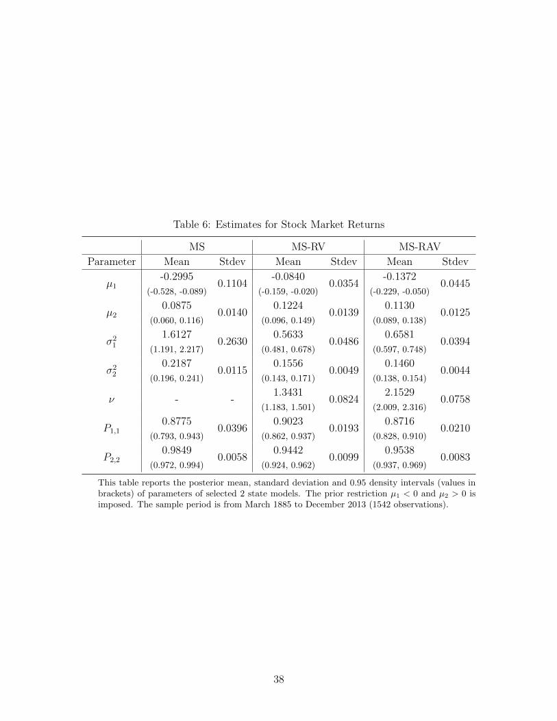
Table 6: Estimates for Stock Market Returns

MS MS-RV MS-RAV

Parameter Mean Stdev Mean Stdev Mean Stdev

µ1-0.2995

0.1104-0.0840

0.0354-0.1372

0.0445(-0.528, -0.089) (-0.159, -0.020) (-0.229, -0.050)

µ20.0875

0.01400.1224

0.01390.1130

0.0125(0.060, 0.116) (0.096, 0.149) (0.089, 0.138)

σ21

1.61270.2630

0.56330.0486

0.65810.0394

(1.191, 2.217) (0.481, 0.678) (0.597, 0.748)

σ22

0.21870.0115

0.15560.0049

0.14600.0044

(0.196, 0.241) (0.143, 0.171) (0.138, 0.154)

ν - -1.3431

0.08242.1529

0.0758(1.183, 1.501) (2.009, 2.316)

P1,10.8775

0.03960.9023

0.01930.8716

0.0210(0.793, 0.943) (0.862, 0.937) (0.828, 0.910)

P2,20.9849

0.00580.9442

0.00990.9538

0.0083(0.972, 0.994) (0.924, 0.962) (0.937, 0.969)

This table reports the posterior mean, standard deviation and 0.95 density intervals (values inbrackets) of parameters of selected 2 state models. The prior restriction µ1 < 0 and µ2 > 0 isimposed. The sample period is from March 1885 to December 2013 (1542 observations).

38

Table 7: Performance of Market Timing Portfolios

Panel A: Jan. 1951 - Dec. 2013

Number of states Model Mean St. Dev. Sharpe Ratio ∆q ∆e

Buy-Hold 0.0826 0.5148 0.1604 - -

2 StatesMS 0.0663 0.4198 0.1578 - -

MS-RV 0.0720 0.3929 0.1831 92.256 96.192

4 StatesMS 0.0690 0.4427 0.1560 -7.188 -4.512

MS-RV 0.0698 0.4040 0.1729 55.860 60.372

-IHMM 0.0657 0.4414 0.1487 -37.608 -37.884

IHMM-RV 0.0770 0.4348 0.1770 82.392 87.888

Panel B: Jan. 1984 - Dec. 2013

Number of states Model Mean St. Dev. Sharpe Ratio ∆q ∆e

Buy-Hold 0.0911 0.5408 0.1684 - -

2 StatesMS 0.0564 0.4755 0.1187 - -

MS-RV 0.0772 0.3909 0.1975 325.536 337.728

4 StatesMS 0.0684 0.4845 0.1412 100.476 108.540

MS-RV 0.0645 0.4291 0.1502 145.476 156.852

-IHMM 0.0563 0.4975 0.1132 -37.212 -37.692

IHMM-RV 0.0794 0.4590 0.1729 247.956 261.276

The summary statistics are based on annualized returns. The values in the last two columns are annu-alized basis point performance fees that an investor is willing to pay to switch away from the 2-stateMarkov switching model to the one in the respective row. ∆q is annualized basis point performancefee based on quadratic utility and ∆e is the performance fee for investor with exponential utility. Therisk aversion coefficient is γ = 5. Bold numbers indicate the largest Sharpe ratio and the largestperformance fee for a class of models.

Table 8: Prior Specification of Multivariate Models

Panel A: Priors for Multivariate MS Models

Model Mst Σst κ Pj

MS N(0, 5I) IW(Cov(Rt), 5) - Dir(1, . . . , 1)

MS-RCOV N(0, 5I) W(13RCOVt, 3) G(20, 1)1κ>4 Dir(1, . . . , 1)

Panel B: Priors for Multivariate IHMM Models

Model Mst Σst κ η α

IHMM N(0, 5I) IW(Cov(Rt), 5) - G(1, 4) G(1, 4)

IHMM-RCOV N(0, 5I) W(13RCOVt, 3) G(20, 1)1κ>4 G(1, 4) G(1, 4)

0 denotes zero vector, I is the identity matrix. Cov(Rt), and RCOVt are computed using in sampledata.

39

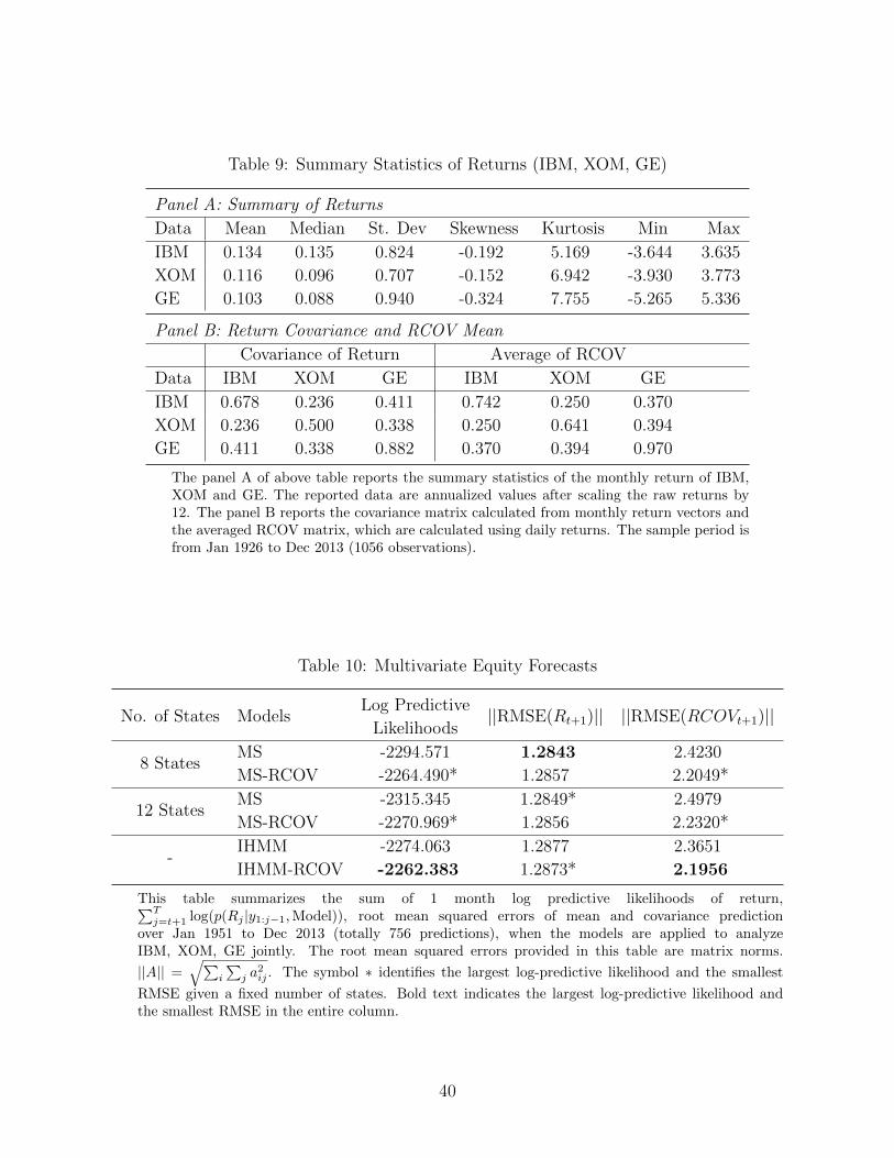
Table 9: Summary Statistics of Returns (IBM, XOM, GE)

Panel A: Summary of Returns

Data Mean Median St. Dev Skewness Kurtosis Min Max

IBM 0.134 0.135 0.824 -0.192 5.169 -3.644 3.635

XOM 0.116 0.096 0.707 -0.152 6.942 -3.930 3.773

GE 0.103 0.088 0.940 -0.324 7.755 -5.265 5.336

Panel B: Return Covariance and RCOV Mean

Covariance of Return Average of RCOV

Data IBM XOM GE IBM XOM GE

IBM 0.678 0.236 0.411 0.742 0.250 0.370

XOM 0.236 0.500 0.338 0.250 0.641 0.394

GE 0.411 0.338 0.882 0.370 0.394 0.970

The panel A of above table reports the summary statistics of the monthly return of IBM,XOM and GE. The reported data are annualized values after scaling the raw returns by12. The panel B reports the covariance matrix calculated from monthly return vectors andthe averaged RCOV matrix, which are calculated using daily returns. The sample period isfrom Jan 1926 to Dec 2013 (1056 observations).

Table 10: Multivariate Equity Forecasts

No. of States ModelsLog Predictive ||RMSE(Rt+1)|| ||RMSE(RCOVt+1)||

Likelihoods

8 StatesMS -2294.571 1.2843 2.4230

MS-RCOV -2264.490* 1.2857 2.2049*

12 StatesMS -2315.345 1.2849* 2.4979

MS-RCOV -2270.969* 1.2856 2.2320*

-IHMM -2274.063 1.2877 2.3651

IHMM-RCOV -2262.383 1.2873* 2.1956

This table summarizes the sum of 1 month log predictive likelihoods of return,∑Tj=t+1 log(p(Rj |y1:j−1,Model)), root mean squared errors of mean and covariance prediction

over Jan 1951 to Dec 2013 (totally 756 predictions), when the models are applied to analyzeIBM, XOM, GE jointly. The root mean squared errors provided in this table are matrix norms.

||A|| =√∑

i

∑j a

2ij . The symbol ∗ identifies the largest log-predictive likelihood and the smallest

RMSE given a fixed number of states. Bold text indicates the largest log-predictive likelihood andthe smallest RMSE in the entire column.

40

Table 11: Performance of Minimum Variance Portfolios (Jan. 1951 - Dec. 2013)

Panel A: Required Annualized Portfolio Return: 10%

Mean St. Dev. Sharpe Ratio ∆q ∆e

8 StatesMS 0.1103 0.3296 0.3345 - -

MS-RCOV 0.1090 0.3155 0.3455 7.080 3.888

12 StatesMS 0.1103 0.3369 0.3273 -10.704 -10.188

MS-RCOV 0.1084 0.3137 0.3456 3.744 0.900

-IHMM 0.1081 0.3257 0.3320 -15.924 -16.224

IHMM-RCOV 0.1089 0.3170 0.3436 4.188 0.600

Panel B: Required Annualized Portfolio Return: 20%

Mean St. Dev. Sharpe Ratio ∆q ∆e

8 StatesMS 0.1956 0.8916 0.2194 - -

MS-RCOV 0.1962 0.8660 0.2265 106.752 83.784

12 StatesMS 0.1934 0.9161 0.2111 -123.468 -116.364

MS-RCOV 0.1970 0.8626 0.2284 128.772 103.104

-IHMM 0.1933 0.8715 0.2218 56.940 45.876

IHMM-RCOV 0.1985 0.8695 0.2283 116.520 90.996

The summary statistics are based on annualized return (scaled by 12). ∆q is annualized basispoint performance fees that an investor with quadratic utility is willing to pay to switch fromthe 8-state MS model. ∆e is the fee for investor with exponential utility. The risk aversioncoefficients are both utility function are γ = 5. Panel A and B shows the results of portfolio with10% and 20% required return, respectively. Out of sample period: Jan 1951 - Dec 2013, totally756 months. Bold numbers indicate the largest Sharpe ratio and the largest performance fee fora class of models.

41

Table 12: Performance of Minimum Variance Portfolios (Jan. 1984 - Dec. 2013)

Panel A: Required Annualized Portfolio Return: 10%

Mean St. Dev. Sharpe Ratio ∆q ∆e

8 StatesMS 0.0907 0.3370 0.2692 - -

MS-RCOV 0.0925 0.3239 0.2856 36.612 33.060

12 StatesMS 0.0889 0.3491 0.2545 -36.708 -36.336

MS-RCOV 0.0938 0.3222 0.2912 51.936 48.348

-IHMM 0.0936 0.3354 0.2791 30.972 33.420

IHMM-RCOV 0.0925 0.3232 0.2860 36.948 32.880

Panel B: Required Annualized Portfolio Return: 20%

Mean St. Dev. Sharpe Ratio ∆q ∆e

8 StatesMS 0.1788 0.9140 0.1956 - -

MS-RCOV 0.1833 0.8934 0.2052 128.520 99.360

12 StatesMS 0.1728 0.9542 0.1811 -229.368 -217.260

MS-RCOV 0.1869 0.8857 0.2110 195.588 161.340

-IHMM 0.1871 0.8966 0.2087 153.588 154.812

IHMM-RCOV 0.1831 0.8967 0.2042 113.532 75.228

The summary statistics are based on annualized return (scaled by 12). ∆q is annualized basispoint performance fees that an investor with quadratic utility is willing to pay to switch fromthe 8-state MS model. ∆e is the fee for investor with exponential utility. The risk aversioncoefficients for both utility function are γ = 5. Panel A and B shows the results of portfolio with10% and 20% required return, respectively. Out of sample period: Jan 1984 - Dec 2013, totally360 months. Bold numbers indicate the largest Sharpe ratio and the largest performance fee fora class of models.

42

Table 13: Return Variances of Global Minimum Variance Portfolios

Panel A: Jan. 1951 - Dec. 2013

No. of States Model Variance

8 StatesMS 0.31123

MS-RCOV 0.29601

12 StatesMS 0.32271

MS-RCOV 0.29191

-IHMM 0.30325

IHMM-RCOV 0.29675

Panel B: Jan. 1984 - Dec. 2013

No. of States Model Variance

8 StatesMS 0.31498

MS-RCOV 0.31112

12 StatesMS 0.33399

MS-RCOV 0.30378

-IHMM 0.31098

IHMM-RCOV 0.31047

This table reports variances of annualized return ofglobal minimum variance portfolios based on com-peting models. Bold numbers indicate the smallestportfolio variance for a class of models.

43

-2

-1

0

1

2

log-P

L D

iffe

rence

0

4

8

12

16

20

24

Cum

ula

tive log-P

L D

iffe

rence

0

1

2

3

1951/01 1961/01 1971/01 1981/01 1991/01 2001/01 2011/01

RA

V

Figure 1: The top panel shows log (p(rt+1|y1:t, IHMM-RV)) − log (p(rt+1|y1:t, IHMM)) overJanuary 1984 to December 2013. The second panel plots the cumulative log-predictivelikelihood difference. The final panel is the time series plot of realized absolute variation.

44

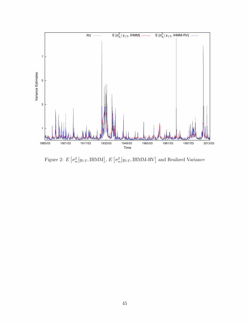
1

3

5

7

1885/03 1901/03 1917/03 1933/03 1949/03 1965/03 1981/03 1997/03 2013/03

Varian

ce E

stim

ate

s

Time

RV E [σst

2 | y1:T, IHMM] E [σst

2 | y1:T, IHMM-RV]

Figure 2: E[σ2st

∣∣y1:T , IHMM], E[σ2st

∣∣y1:T , IHMM-RV]

and Realized Variance

45

10

30

50

70

Lo

g P

rice I

nde

x

0

0.2

0.4

0.6

0.8

1

MS

0

0.2

0.4

0.6

0.8

1

MS

-RV

0

0.2

0.4

0.6

0.8

1

1885/03 1901/03 1917/03 1933/03 1949/03 1965/03 1981/03 1997/03 2013/03

MS

-RA

V

Time

Figure 3: Smoothed Probability of High Return State

46

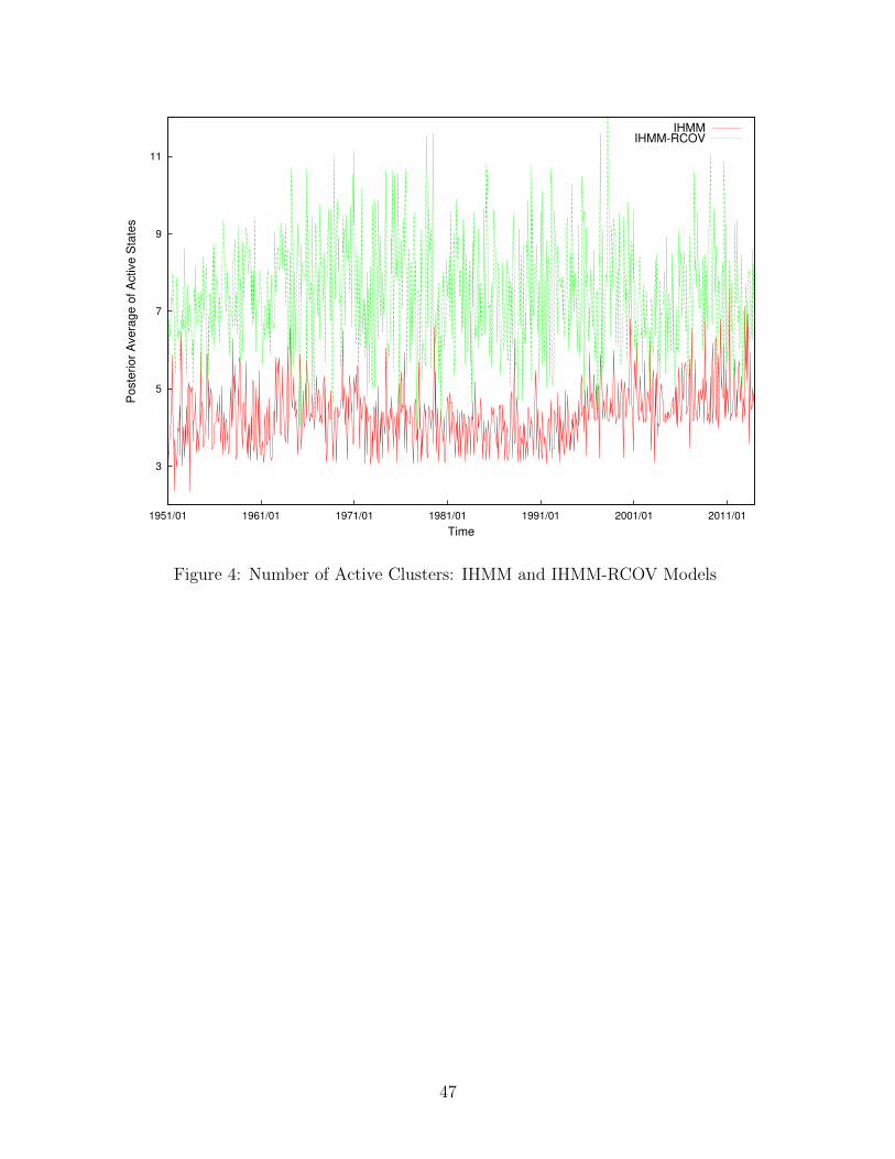
3

5

7

9

11

1951/01 1961/01 1971/01 1981/01 1991/01 2001/01 2011/01

Poste

rio

r A

ve

rag

e o

f A

ctive S

tate

s

Time

IHMMIHMM-RCOV

Figure 4: Number of Active Clusters: IHMM and IHMM-RCOV Models

47