introduction to markov-switching regression models using ... · introduction to markov-switching...
TRANSCRIPT
Introduction to Markov-switching regression modelsusing the mswitch command
Gustavo Sánchez
StataCorp
May 18, 2016Aguascalientes, México
(StataCorp) Markov-switching regression in Stata May 18 1 / 1

Introduction to Markov-switching regression modelsusing the mswitch command
Gustavo Sánchez
StataCorp
May 18, 2016Aguascalientes, México
(StataCorp) Markov-switching regression in Stata May 18 2 / 1

Outline
1 When we use Markov-Switching Regression Models
2 Introductory concepts
3 Markov-Switching Dynamic RegressionPredictions
State probabilities predictionsLevel predictions
State expected durationsTransition probabilities
4 Markov-Switching AR Models
(StataCorp) Markov-switching regression in Stata May 18 3 / 1
When we use Markov-Switching Regression Models
The parameters of the data generating process (DGP) vary over aset of different unobserved states.
We do not know the current state of the DGP, but we can estimatethe probability of each possible state.
(StataCorp) Markov-switching regression in Stata May 18 4 / 1
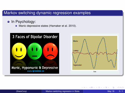
Markov switching dynamic regression examples
In Psychology:Manic depressive states (Hamaker et al. 2010).
(StataCorp) Markov-switching regression in Stata May 18 5 / 1

Markov switching dynamic regression examples
In Economics:Asymmetrical behavior over GDP expansions and recessions (Hamilton 1989).Exchange rates (Engel and Hamilton 1990).Interest rates (García and Perron 1996).Stock returns (Kim et al. 1998).
(StataCorp) Markov-switching regression in Stata May 18 6 / 1

Markov switching dynamic regression examples
In Epidemiology:Incidence rates of infectious disease in epidemic and nonepidemic states (Lu et al.2010).
Source:http://www.slideshare.net/meningitis/1620-mrf-marie-pierre-preziosi-06-nov
(StataCorp) Markov-switching regression in Stata May 18 7 / 1

Markov switching dynamic regression examples
In Political Science:Democratic and Republican partisan states in the US congress (Jones et al 2010).
State 1: Republicans are the dominant national partyState 2: Democrats are the dominant national party
(StataCorp) Markov-switching regression in Stata May 18 8 / 1

When we use Markov-Switching Regression Models
The time series in all those examples are characterized by DGPswith dynamics that are state dependent.
States may be recessions and expansions, high/low volatility,depressive/non-depressive, epidemic/non-epidemic states, etc.
Any of the parameters (beta estimates, sigma, AR components)may be different for each state.
(StataCorp) Markov-switching regression in Stata May 18 9 / 1

Different volatilities Mexican peso to Us dollar
(StataCorp) Markov-switching regression in Stata May 18 10 / 1

Different levels, volatilities and slopes- West Texas Oil Price
(StataCorp) Markov-switching regression in Stata May 18 11 / 1

Different AR structure - Interbank interest rate for Spain
(StataCorp) Markov-switching regression in Stata May 18 12 / 1

Introductory Concepts
(StataCorp) Markov-switching regression in Stata May 18 13 / 1
Markov-Switching Regression Models
Models for time series that transition over a set of finiteunobserved states.
The time of transition between states and the duration in aparticular state are both random.
The transitions follow a Markov process.
We can estimate state-dependent and state-independentparameters.
(StataCorp) Markov-switching regression in Stata May 18 14 / 1

Markov-Switching Regression Models
Let’s then define a (first order) Markov Chain:
Assume the states are defined by a random variable St that takesthe integer values 1, 2, ..., N.
Then, the probability of the current state, j, only depends on theprevious state:
P(St = j |St−1 = i ,St−2 = k ,St−3 = w ...) = P(St = j |St−1 = i) = pij
(StataCorp) Markov-switching regression in Stata May 18 15 / 1

Markov-Switching Regression Models
Let’s define a simple constant only model with three states:
yt = µst + εt
Where:µst = µ1 if st = 1µst = µ2 if st = 2µst = µ3 if st = 3
We do not know with certainty the current state, but we canestimate the probability of being in each state.
We can also estimate the transition probabilities:pij : probability of being in state j in the current period given that theprocess was in state i in the previous period.
(StataCorp) Markov-switching regression in Stata May 18 16 / 1

Transition probabilities, expected duration, tests
We will then be interested in obtaining the matrix with thetransition probabilities: p11 p12 p13
p21 p22 p23p31 p32 p33
Where:
p11 + p12 + p13 = 1p21 + p22 + p23 = 1p31 + p32 + p33 = 1
We will also be interested in the expected duration for each state.
We can perform tests for comparing parameters across states
(StataCorp) Markov-switching regression in Stata May 18 17 / 1

Markov-switching dynamic regression
(StataCorp) Markov-switching regression in Stata May 18 18 / 1

Markov-switching dynamic regression
Allow states to switch according to a Markov process
Allow for quick adjustments after a change of state.
Often applied to high frequency data (monthly,weekly,etc.)
(StataCorp) Markov-switching regression in Stata May 18 19 / 1

Markov-switching dynamic regression
The model can be written as:
yt = µst + xtα+ ztβst + εt
Where:
yt : Dependent variable
xt : Vector of exog. variables with state invariant coefficients α
zt : Vector of exog. variables with state-dependent coefficients βs
εst ~iid N(0, σ2s )
We can also include lags of the dependent variable among theregressors
(StataCorp) Markov-switching regression in Stata May 18 20 / 1

Markov switching dynamic regression
Example 1:Mexican peso to US dollarPeriod: 1989m1 - 2015m12Source: Banco de México
(StataCorp) Markov-switching regression in Stata May 18 21 / 1

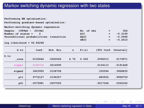
Markov switching dynamic regression with two states
. mswitch dr D.tc,states(2) varswitch switch(,noconstant) constant nolog
Performing EM optimization:
Performing gradient-based optimization:
Markov-switching dynamic regression
Sample: 1989m2 - 2016m1 No. of obs = 324Number of states = 2 AIC = -0.3199Unconditional probabilities: transition HQIC = -0.2966
SBIC = -0.2615Log likelihood = 56.82268
D.tc Coef. Std. Err. z P>|z| [95% Conf. Interval]
D.tc_cons .0135642 .0020066 6.76 0.000 .0096313 .0174971
sigma1 .0160312 .0014595 .0134113 .0191628
sigma2 .3603955 .0158708 .330594 .3928835
p11 .9772127 .0196357 .883934 .9958759
p21 .0075981 .0057055 .0017346 .0326345
(StataCorp) Markov-switching regression in Stata May 18 22 / 1

Markov switching dynamic regression with two states
Probabilities of being in a given state
. predict pr_state1 pr_state2, pr
(StataCorp) Markov-switching regression in Stata May 18 23 / 1

MSDR - Example 1: Probability of being in State 1
(StataCorp) Markov-switching regression in Stata May 18 24 / 1
Markov switching dynamic regression with two states
Performing EM optimization:
Performing gradient-based optimization:
Markov-switching dynamic regression
Sample: 1989m2 - 2016m1 No. of obs = 324Number of states = 2 AIC = -0.3199Unconditional probabilities: transition HQIC = -0.2966
SBIC = -0.2615Log likelihood = 56.82268
D.tc Coef. Std. Err. z P>|z| [95% Conf. Interval]
D.tc_cons .0135642 .0020066 6.76 0.000 .0096313 .0174971
sigma1 .0160312 .0014595 .0134113 .0191628
sigma2 .3603955 .0158708 .330594 .3928835
p11 .9772127 .0196357 .883934 .9958759
p21 .0075981 .0057055 .0017346 .0326345
(StataCorp) Markov-switching regression in Stata May 18 25 / 1

MSDR - Example 1: Probability of being in State 2
(StataCorp) Markov-switching regression in Stata May 18 26 / 1

Markov switching dynamic regression with two states
Performing EM optimization:
Performing gradient-based optimization:
Markov-switching dynamic regression
Sample: 1989m2 - 2016m1 No. of obs = 324Number of states = 2 AIC = -0.3199Unconditional probabilities: transition HQIC = -0.2966
SBIC = -0.2615Log likelihood = 56.82268
D.tc Coef. Std. Err. z P>|z| [95% Conf. Interval]
D.tc_cons .0135642 .0020066 6.76 0.000 .0096313 .0174971
sigma1 .0160312 .0014595 .0134113 .0191628
sigma2 .3603955 .0158708 .330594 .3928835
p11 .9772127 .0196357 .883934 .9958759
p21 .0075981 .0057055 .0017346 .0326345
(StataCorp) Markov-switching regression in Stata May 18 27 / 1

Markov switching dynamic regression
Example 2:West Texas Oil PricePeriod: 1974q1 - 2016q1Source: Federal Reserve Bank of St. Louis
(StataCorp) Markov-switching regression in Stata May 18 28 / 1

Markov switching dynamic regression for WTI
. mswitch dr wti,varswitch states(2) switch(L(1/2).wti) nolog vsquishMarkov-switching dynamic regression
Sample: 1974q3 - 2016q1 No. of obs = 167Number of states = 2 AIC = 5.7406Unconditional probabilities: transition HQIC = 5.8163
wti Coef. Std. Err. z P>|z| [95% Conf. Interval]
State1wtiL1. 1.159938 .1420059 8.17 0.000 .8816118 1.438265L2. -.2717729 .1411955 -1.92 0.054 -.548511 .0049652
_cons 7.194071 4.937824 1.46 0.145 -2.483886 16.87203
State2wtiL1. 1.350215 .1098233 12.29 0.000 1.134965 1.565465L2. -.3653538 .10544 -3.47 0.001 -.5720124 -.1586951
_cons .6982948 .5103081 1.37 0.171 -.3018907 1.69848
sigma1 12.33223 1.337368 9.970875 15.25282
sigma2 2.013336 .1763262 1.695777 2.390362
p11 .9061409 .0513983 .7470475 .969287
p21 .0428145 .0223459 .01513 .1152286
(StataCorp) Markov-switching regression in Stata May 18 29 / 1

Markov switching dynamic regression for WTI
Test on the equality of intercept across states. test [State1]L1.wti=[State2]L1.wti,notest( 1) [State1]L.wti - [State2]L.wti = 0
. test [State1]L2.wti=[State2]L2.wti,accum( 1) [State1]L.wti - [State2]L.wti = 0( 2) [State1]L2.wti - [State2]L2.wti = 0
chi2( 2) = 2.61Prob > chi2 = 0.2717
Test on the equality of sigma across states. test [lnsigma1]_cons=[lnsigma2]_cons( 1) [lnsigma1]_cons - [lnsigma2)]_cons = 0
chi2( 1) = 199.07Prob > chi2 = 0.0000
(StataCorp) Markov-switching regression in Stata May 18 30 / 1

Markov switching dynamic regression for WTI
. mswitch dr wti L(1/2).wti, varswitch states(2) nolog vsquishMarkov-switching dynamic regression
Sample: 1974q3 - 2016q1 No. of obs = 167Number of states = 2 AIC = 5.7352Unconditional probabilities: transition HQIC = 5.7958
wti Coef. Std. Err. z P>|z| [95% Conf. Interval]
wtiwtiL1. 1.189054 .1192115 9.97 0.000 .9554034 1.422704L2. -.2494644 .1099147 -2.27 0.023 -.4648932 -.0340356
State1_cons 3.837488 2.213145 1.73 0.083 -.5001956 8.175171
State2_cons 1.441643 .5538878 2.60 0.009 .3560428 2.527243
sigma1 11.06814 1.179045 8.982545 13.63797
sigma2 1.759657 .2833698 1.283374 2.412698
p11 .9394488 .0337386 .8291112 .9802425
p21 .0392075 .022843 .0122803 .1181172
(StataCorp) Markov-switching regression in Stata May 18 31 / 1

Markov switching dynamic regression
Predict probabilities of being at each state
predict pr_state1 pr_state2, pr
(StataCorp) Markov-switching regression in Stata May 18 32 / 1

MSDR - Example 2: Probability of being in State 1
(StataCorp) Markov-switching regression in Stata May 18 33 / 1

Markov switching dynamic regression for WTI
Markov-switching dynamic regression
Sample: 1974q3 - 2016q1 No. of obs = 167Number of states = 2 AIC = 5.7352Unconditional probabilities: transition HQIC = 5.7958
wti Coef. Std. Err. z P>|z| [95% Conf. Interval]
wtiwtiL1. 1.189054 .1192115 9.97 0.000 .9554034 1.422704L2. -.2494644 .1099147 -2.27 0.023 -.4648932 -.0340356
State1_cons 3.837488 2.213145 1.73 0.083 -.5001956 8.175171
State2_cons 1.441643 .5538878 2.60 0.009 .3560428 2.527243
sigma1 11.06814 1.179045 8.982545 13.63797
sigma2 1.759657 .2833698 1.283374 2.412698
p11 .9394488 .0337386 .8291112 .9802425
p21 .0392075 .022843 .0122803 .1181172
(StataCorp) Markov-switching regression in Stata May 18 34 / 1
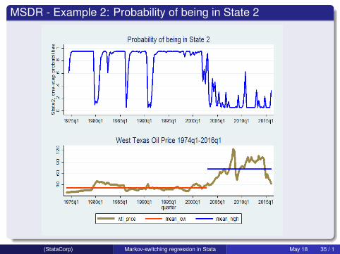
MSDR - Example 2: Probability of being in State 2
(StataCorp) Markov-switching regression in Stata May 18 35 / 1

Markov switching dynamic regression for WTI
Markov-switching dynamic regression
Sample: 1974q3 - 2016q1 No. of obs = 167Number of states = 2 AIC = 5.7352Unconditional probabilities: transition HQIC = 5.7958
wti Coef. Std. Err. z P>|z| [95% Conf. Interval]
wtiwtiL1. 1.189054 .1192115 9.97 0.000 .9554034 1.422704L2. -.2494644 .1099147 -2.27 0.023 -.4648932 -.0340356
State1_cons 3.837488 2.213145 1.73 0.083 -.5001956 8.175171
State2_cons 1.441643 .5538878 2.60 0.009 .3560428 2.527243
sigma1 11.06814 1.179045 8.982545 13.63797
sigma2 1.759657 .2833698 1.283374 2.412698
p11 .9394488 .0337386 .8291112 .9802425
p21 .0392075 .022843 .0122803 .1181172
(StataCorp) Markov-switching regression in Stata May 18 36 / 1

Markov switching dynamic regression for WTI
Transition probabilities. estat transition
Number of obs = 167
Transition Probabilities Estimate Std. Err. [95% Conf. Interval]
p11 .9394488 .0337386 .8291112 .9802425
p12 .0605512 .0337386 .0197575 .1708888
p21 .0392075 .022843 .0122803 .1181172
p22 .9607925 .022843 .8818828 .9877197
(StataCorp) Markov-switching regression in Stata May 18 37 / 1

Markov switching dynamic regression for WTI
Expected duration. estat duration
Number of obs = 167
Expected Duration Estimate Std. Err. [95% Conf. Interval]
State1 16.51496 9.201998 5.851757 50.61379
State2 25.50535 14.85988 8.466169 81.43109
(StataCorp) Markov-switching regression in Stata May 18 38 / 1

Markov-switching AR model
(StataCorp) Markov-switching regression in Stata May 18 39 / 1

Markov-switching AR model
Allow states to switch according to a Markov process
Allow a gradual adjustment after a change of state.
Often applied to lower frequency data (quarterly, yearly, etc.)
(StataCorp) Markov-switching regression in Stata May 18 40 / 1

Markov-switching AR model
The model can be written as:
yt = µst +xtα+ztβst +P∑
i=1
φi,st (yt−i −µst−i −xt−iα+zt−iβst−i )+ εt ,st
Where:
yt : Dependent variable
µst : State-dependent intercept
xt : Vector of exog. variables with state invariant coefficients α
zt : Vector of exog. variables with state-dependent coefficients βst
φi,st : i th AR term in state st
εt,st ~iid N(0, σ2s )
(StataCorp) Markov-switching regression in Stata May 18 41 / 1

Markov switching AR model
Example 3:Interbank interest rate for SpainPeriod: 1989Q4 - 2015Q3Source: Banco de España
(StataCorp) Markov-switching regression in Stata May 18 42 / 1

Markov switching AR model
. mswitch ar D.r_interbank D.ipc,states(2) ar(1) ///arswitch varswitch switch(,noconstant) constant
Markov-switching autoregression
Sample: 1990q2 - 2012q4 No. of obs = 91Number of states = 2 AIC = 1.1681Unconditional probabilities: transition HQIC = 1.2572
D.r_interbank Coef. Std. Err. z P>|z| [95% Conf. Interval]
D.r_interb~kipcD1. .1345492 .0430415 3.13 0.002 .0501895 .218909
_cons -.1287786 .0299325 -4.30 0.000 -.1874453 -.0701119
State1arL1. -.5821326 .0868487 -6.70 0.000 -.7523529 -.4119122
State2arL1. .600846 .1133802 5.30 0.000 .3786249 .8230671
sigma1 .10039 .021533 .0659346 .1528509
sigma2 .4279839 .0404373 .3556339 .5150526
(StataCorp) Markov-switching regression in Stata May 18 43 / 1

Markov switching AR model
. estat transitionNumber of obs = 91
Transition Probabilities Estimate Std. Err. [95% Conf. Interval]
p11 .6238106 .1906249 .2523082 .8906938
p12 .3761894 .1906249 .1093062 .7476918
p21 .0917497 .0529781 .0282364 .2599153
p22 .9082503 .0529781 .7400847 .9717636
. estat durationNumber of obs = 91
Expected Duration Estimate Std. Err. [95% Conf. Interval]
State1 2.658235 1.346997 1.33745 9.148609
State2 10.89922 6.293423 3.847408 35.41533
(StataCorp) Markov-switching regression in Stata May 18 44 / 1

MSAR - Example 3: Probability of being in each State
(StataCorp) Markov-switching regression in Stata May 18 45 / 1

Markov switching AR model
. predict state*,yhat dynamic(tq(2012q4))
. forvalues i=1/2 {2. generate y_st`i´=state`i´+L.r_interbank3. }
(StataCorp) Markov-switching regression in Stata May 18 46 / 1

Markov switching AR model
. predict r_hat,yhat dynamic(tq(2012q4))
(StataCorp) Markov-switching regression in Stata May 18 47 / 1
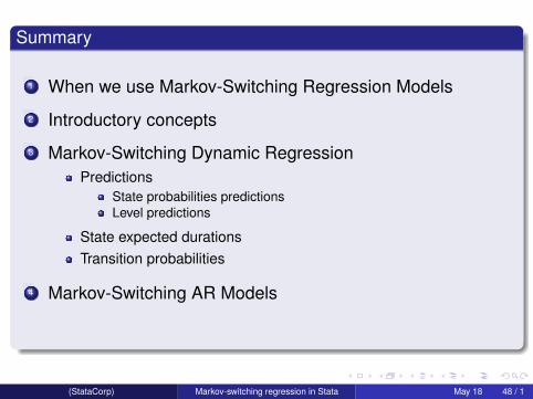
Summary
1 When we use Markov-Switching Regression Models
2 Introductory concepts
3 Markov-Switching Dynamic RegressionPredictions
State probabilities predictionsLevel predictions
State expected durationsTransition probabilities
4 Markov-Switching AR Models
(StataCorp) Markov-switching regression in Stata May 18 48 / 1

References
Engel, C., and J. D. Hamilton. 1990. Long swings in the dollar: Are they in thedata and do markets know it?. American Economic Review 80: 689—713.Hamilton, J. D. 1989. A new approach to the economic analysis of nonstationarytime series and the business cycle. Econometrica 57: 357—384.Garcia, R., and P. Perron. 1996. An analysis of the real interest rate underregime shifts. Review of Economics and Statistics 78: 111—125.Kim, C.-J., C. R. Nelson, and R. Startz. 1998. Testing for mean reversion inheteroskedastic data based on Gibbs-sampling-augmented randomization.Journal of Empirical Finance 5: 115—43.Lu, H.-M., D. Zeng, and H. Chen. 2010. Prospective infectious disease outbreakdetection using Markov switching models. IEEE Transactions on Knowledge andData Engineering 22: 565—577.Hamaker, E. L., R. P. P. P. Grasman, and J. H. Kamphuis. 2010.Regime-switching models to study psychological processes. In IndividualPathways of Change: Statistical Models for Analyzing Learning andDevelopment, ed. P. C. Molenaar and K. M. Newell, 155—168. Washington, DC:American Psychological Association
(StataCorp) Markov-switching regression in Stata May 18 49 / 1