three essays on transportation, energy, and supply...
TRANSCRIPT

THREE ESSAYS ON TRANSPORTATION, ENERGY, AND SUPPLY CHAIN FINANCE
ECONOMICS
By
XIAODONG LANG
A dissertation submitted in partial fulfillment ofthe requirements for the degree of
DOCTOR OF PHILOSOPHY
WASHINGTON STATE UNIVERSITYSchool of Economic Sciences
MAY 2019
c© Copyright by XIAODONG LANG, 2019All Rights Reserved

c© Copyright by XIAODONG LANG, 2019All Rights Reserved

To the Faculty of Washington State University:
The members of the Committee appointed to examine the dissertation of XIAODONG
LANG find it satisfactory and recommend that it be accepted.
H. Alan Love, Ph.D., Chair
Eric L. Jessup, Ph.D., Co-Chair
Vicki A. McCracken, Ph.D.
Jinhui Bai, Ph.D.
ii

ACKNOWLEDGMENT
Firstly, I would like to express my sincere gratitude to my advisors Dr. Alan Love and Dr.
Eric Jessup for the continuous support of my Ph.D study and related research, for their patience,
motivation, and immense knowledge. Their guidance helped me in all the time of research and
writing of this thesis.
Besides my advisors,I would like to grant special gratitude to Dr. Vicki McCraken for her
continuous inspiration on me since I was a undergraduate student in Washington State University.
I could not have imagined having a better advisor and mentor for my entire student life.
I would also like to thank Dr. Jinhui Bai, for his insightful comments and suggestions, which
have substantially shaped and improved my dissertation.
I thank my fellow colleagues at Washington State University, especially Xiangrui Wang, Xin-
long Tan, Zhuang Hao, Ziying Yang, and Haowei Yu, for the support and encouragement over the
challenging moments and for their friendship.
Last but not least, I would like to thank my parents Hongjin Lang and Jingzhen Sun, parents
in law Xingzhao Li and Jing Li, and specially my two princesses Olivia and Grace for everything,
including supporting me spiritually throughout finishing this dissertation and pursuing my Ph.D.
iii

THREE ESSAYS ON ENERGY, TRANSPORTATION, AND SUPPLY CHAIN FINANCE
ECONOMICS
Abstract
by Xiaodong Lang, Ph.D.Washington State University
May 2019
Chair: H. Alan Love; Co-Chair: Eric L. Jessup
This dissertation contains three independent chapters in the field of transportation, energy and
supply chain finance economics. The first paper applies an ordered probit model to examine how
the availability of commercial truck parking potentially affects the injury severity of commercial
vehicle drivers normalized for other driving-related and environmental factors. The second paper
aims to identify the impacts on retail electricity price after retail electricity market was restructured
in the United States. The third paper aims to identify the impacts on manufacturing firms’ financial
performance with supplier diversification.
iv

TABLE OF CONTENTS
Page
ACKNOWLEDGMENT.............................................................................................................. iii
ABSTRACT................................................................................................................................. iv
LIST OF TABLES ....................................................................................................................... viii
LIST OF FIGURES ..................................................................................................................... ix
CHAPTER ONE
CHAPTER TWO
1. INTRODUCTION......................................................................................................... 4
2. LITERATURE REVIEW.............................................................................................. 5
3. DATA ............................................................................................................................ 8
3.1 SOURCE OF DATA ......................................................................................... 8
3.2 DEPENDENT VARIABLE.............................................................................. 9
3.3 EXPLANTORY VARIABLE ........................................................................... 9
4. METHODOLOGY........................................................................................................ 10
5. RESULTS AND DISCUSSION ................................................................................... 12
5.1 ESTIMATION RESULTS ................................................................................ 12
5.2 GROUP ONE: GVWR GREATER THAN 26,000 lbs .................................... 12
5.3 GROUP TWO: GVWR BETWEEN 10,001 lbs AND 26,000 lbs ................... 14
v

5.4 ANALYSIS OF MARGINAL EFFECTS......................................................... 14
5.5 DISCUSSION AND IMPLICATIONS ............................................................ 15
6. CONCLUSION............................................................................................................. 16
CHAPTER THREE
1. INTRODUCTION......................................................................................................... 22
2. DATA ............................................................................................................................ 25
2.1 DEPENDENT VARIABLE.............................................................................. 25
2.2 EXPLANTORY VARIABLES......................................................................... 25
2.3 GROUPS AND PERIODS SELECTION FOR SCM ...................................... 26
3. METHODOLOGY........................................................................................................ 27
3.1 THE DIFFERENCE-IN-DIFFERENCE METHOD........................................ 27
3.2 SYNTHETIC CONTROL METHOD(SCM)................................................... 28
3.3 ASSUMPTION................................................................................................. 30
4. RESULTS...................................................................................................................... 31
4.1 RESIDENTIAL RETAIL PRICE..................................................................... 31
4.2 COMMERCIAL RETAIL PRICE.................................................................... 32
4.3 INDUSTRIAL RETAIL PRICE....................................................................... 33
5. CONCLUSION............................................................................................................. 33
CHAPTER FOUR
1. INTRODUCTION......................................................................................................... 40
2. LITERATURE .............................................................................................................. 41
vi

3. DATA ............................................................................................................................ 43
3.1 SAMPLE CONSTRUCTION........................................................................... 43
3.2 DEPENDENT VARIABLE.............................................................................. 44
3.3 EXPLANATORY VARIABLE......................................................................... 44
4. EMPIRICAL REGRESSION AND RESULTS............................................................ 45
4.1 SUPPLIER DIVERSIFICATION ESTIMATION............................................ 45
4.2 CURRENT YEAR V.S. FOLLOWING YEAR ............................................... 47
5. DISCUSSION ............................................................................................................... 49
6. CONCLUSION............................................................................................................. 50
CHAPTER FIVE
REFERENCES ............................................................................................................................ 57
vii

LIST OF TABLES
Table 2.1 Variable Definition and Descriptive Statistics..................................................... 18
Table 2.2 Ordered Probit Model Estimation Results .......................................................... 19
Table 2.3 Marginal Effects of Ordered Probit Model for GVWR 26,000 lbs or more ....... 20
Table 2.4 Marginal Effects of Ordered Probit Model for GVWR 10,001 lbs - 26,000 lbs. 21
Table 3.1 Summary Statistics.............................................................................................. 35
Table 4.1 Summary Statistics.............................................................................................. 52
Table 4.2 Effect of Supplier Diversification on Customer Firms’ Current Year Return ..... 53
Table 4.3 Effect of Supplier Diversification on Customer Firms’ Following Year Return. 54
viii

LIST OF FIGURES
Figure 3.1 Map of U.S. Regional Transmission Organizations .......................................... 36
Figure 3.2 Effects on Residential Retail Price for restructured RSOs/ISOs ....................... 37
Figure 3.3 Effects on Commercial Retail Price for restructured RSOs/ISOs ..................... 38
Figure 3.4 Effects on Industrial Retail Price for restructured RSOs/ISOs.......................... 39
ix

Dedication
This dissertation is dedicated to my wife Zishan Li who encouraged me to pursue my dreams and
finish my dissertation.
x

CHAPTER ONE:
INTRODUCTION OF DISSERTATION
This dissertation contains three independent chapters in the field of transportation, energy and
supply chain finance economics. The first paper applies an ordered probit model to examine how
the availability of commercial truck parking potentially affects the injury severity of commercial
vehicle drivers normalized for other driving-related and environmental factors. The second pa-
per estimates the impacts on retail electricity price after retail electricity market was restructured
in the United States. The third paper focuses on the impacts on manufacturing firms’ financial
performance with supplier diversification.
The rapid growth of freight tonnage has made the availability of adequate commercial park-
ing a national safety issue in the United States. My first paper (Chapter Two) applies an ordered
probit model to examine how the availability or lack there of commercial truck parking potentially
affects the injury severity of commercial vehicle drivers normalized for other driving-related and
environmental factors. The data and information utilized in this study are crash data obtained from
the Fatality Analysis Reporting System (FARS) compiled by the National Highway Traffic Safety
Administration (NHTSA) from 2001 to 2016 for all fifty states and the District of Columbia. Re-
sults suggest that an increase in the total number of parking spots within a thirty-minute driving
distance reduces the probability of a higher degree of injury and increases the probability of less
severe injury. Other factors that increase the probability of severe injuries include adverse sur-
face conditions, night driving, older drivers, male drivers, and drug- or alcohol-related offenses.
This paper addresses a national safety issue related to available truck parking in the United States
and finds a negative relationship between truck accident severity and access to available parking.
Stated differently, improved access and proximity to available parking reduces the severity of truck
accidents.
Starting from late 1990s, a trend of electricity market restructuring swept through around half
1

of the US states. Two decades after the initiation of electricity market restructuring, sixteen states
are still actively engaged deregulating the retail electricity market. However six states have sus-
pended the deregulation process. There is debate of whether introduction of competition into
electricity industry improves efficiency has not ended. The second paper (Chapter Three) aims to
identify the impacts on residential electricity price after retail electricity market has been dereg-
ulated in the United States. The average treatment effect is examined by applying a synthetic
control method that is integrated with generalized linear models. Control variables are included
in the model to adjust for factors that violate the parallel trend assumption. Deregulated states
are grouped and analyzed into five Regional Transmission Organizations (RTO) including Inde-
pendent System Operator New England (ISO-NE), Mid-continent Independent System Operator
(MISO), New York Independent System Operator (NYISO), PJM Interconnection (PJM), Electric
Reliability Council of Texas (ERCOT). Oregon state is analyzed separately. The main finding is
that impacts vary by location and design of the electricity market restructuring. ISO-NE, MISO,
NYISO, and PJM all show significant decreases in retail, commercial, and industrial residential
electricity price compared to the synthetic group, while ERCOT indicates a relatively higher price.
The treatment effect analysis does not highlight any change of price for Oregon state. This paper
is the first application of a synthetic control method to analyze the impact of electricity market
restructuring. The different results within RTOs reveal that different approaches to electricity mar-
ket restructuring resulting in varying outcomes, which is important to both policy makers and
researchers.
In recent years, the business community has recognized the need to mange the supply chain as
part of broader business strategies, and in particular to build and exploit collaborative relationships
with supply chain partners. The third paper (Chapter Four) identifies the impacts on customers’
financial performance with supplier diversification. The diversification of suppliers is captured by
the number and shares of suppliers with related customer firms. Short-term and long-term impacts
are examined in this research. Results suggest that the downstream firms’ return increase with an
increase of the number of suppliers, fallen major suppliers share percentage increase, and with the
2

occurrence of major supplier change.
3

CHAPTER TWO:
AN ANALYSIS OF DRIVER’S INJURY SEVERITY RELATED TO COMMERCIAL
TRUCK PARKING AVAILABILITY
1. INTRODUCTION
In the United States, the availability of adequate commercial truck parking and the consequences of
parking shortages are significant national safety issues. A 2012 study by the Federal Highway Ad-
ministration (FHWA) reports that a shortage of parking for commercial truck presents a significant
and dangerous problem Tefft (2010). The Freight Analysis Framework (FAF 3.4) projects a future
freight tonnage growth of more than 51 percent between 2007 and 2040. Recent improvements
in U.S. economic growth have led to an increasing demand for truck freight, leading to increasing
truck rates at the national level and within key markets. As truck freight traffic increases, the need
for safe and legal commercial truck parking demand also rises. According to the existing Hours-of-
Service (HOS) regulations issued by the Federal Motor Carrier Safety Administration (FMCSA),
truck drivers are restricted to driving for no more than 11 consecutive hours. Additionally, HOS
limits driving to 60/70 total hours over 7 or 8 consecutive days. Given these HOS regulations,
the limited availability of commercial truck parking may exacerbate safety issues for the drivers
of commercial vehicles. Moreover, when the pending Electronic Log Device requirement by the
Federal Motor Carrier Safety Administration takes effect, truck drivers will no longer be able to
manually adjust driving logs, which will place greater limits on freight capacity and increase the
demand for available parking.
The driver HOS limits the driving hours due to concerns about the effects of fatigue and dis-
traction during long driving hours. If at a particular location there are no available parking spots
for freight vehicles, the driver usually must choose between driving to the next available parking
locations or parking illegally on shoulders and ramps along highway segments. Approximately
16.5% of fatal traffic accidents and 12.5% of collisions that lead to injuries in the United States are
4

related to fatigue driving Tefft (2010). A 2006 study by the Federal Motor Carrier Safety Adminis-
tration found that fatigue was the sixth largest driver-related factor in truck crashes, involving 13%
of all truck crashes Administration (2006).
Prior research studies have estimated the attributes that contribute to truck crashes (Taylor
et al. 1999, Morris et al. 2018, Banerjee et al. 2009,and Bunn et al. 2017). Moving beyond this
approach, our article focuses on the relationship between truck accident severity (as measured
by injuries to the truck driver) and a variety of influential variables, including proximity of the
accident to available truck parking. We select as our estimation technique the discrete order probit
model because of the ordinal nature of injury severity data. This model controls for a variety of
driver, crash, and external characteristics, thus offering new insights into the factors that contribute
to truck driver accident severity.
The remainder of the paper is organized as follows. The related literature is summarized in
Section 2. Section 3 presents the explanation of the source and selection of data. Section 4 explains
the methodology of Order Probit Model in details. Section 5 summarizes the results and discusses
the possible implications of the findings for policy. Section 6 concludes the main findings and
contribution of this research.
2. LITERATURE REVIEW
The Federal Highway Administration (FHWA) reported in 2012 that the lack of adequate commer-
cial truck parking remained a significant and dangerous problem Tefft (2010). The study concludes,
first, that the existing demand for commercial truck parking spaces exceeded the current available
supply, and, second, that the forecasted increase in vehicle miles traveled would exponentially
aggravate the problem.
Taylor et al. (1999) analyze the relationship between the spacing of rest areas and vehicle
crashes on Michigan interstate highways. They develop a hazard function to measure the proba-
bility that a crash will occur in a predetermined distance interval from the previous rest area, while
5

controlling for various confounding traffic and roadway factors. The results indicate a positive
relationship between safety rest-area spacing and fatigue-related single-vehicle truck crashes. As
the spacing between rest areas increases, single-vehicle truck crashes increase during nighttime
(i.e., 10:00 PM to 6:00 AM). Moreover, the frequency of single-vehicle truck crashes increases
with increases in the percentage of spaces filled at rest areas, suggesting that shortages of parking
spaces increase single-truck crash frequency.
Expanding on Taylor et al. (1999) estimation, Morris and O’Brien (2007) include additional
comprehensive variables to control for other potential confounding factors, such as vehicle charac-
teristics and weather conditions. Examining crashes incidents from key interstates in Minnesota,
Morris and O’Brien (2007), find a significant positive statistical correlation between single-vehicle
truck crashes and safety rest-area occupancy, according to a regression analysis. To validate their
results, they employ three measures of rest occupancy: (1) spacing between safety rest areas; (2)
the occupancy of safety rest areas; and (3) the nighttime safety rest-area occupancy rate. Note that
adding extra variables does not guarantee the explanatory power, measured by R2, of the Morris
and O’Brien (2007) approach.
In addition to validating the results reported by the two studies discussed above, Banerjee et al.
(2009) improve the research design in two areas. First, they distinguish between collisions that
occurred 10 miles either upstream or downstream from the rest areas. The results indicate that
the downstream fatigue-related collision rate declines immediately outside the rest area, but rises
sharply after 30 miles, while the non-fatigue-related collisions rate remains consistent. Second,
they propose two alternative definitions of fatigue-related crashes: “strict” and “expanded” fatigue-
related crashes. The results remain robust. 1
Lee and Abdel-Aty (2008) utilized the Large Truck Crash Causation Study (LTCCS) to esti-
mate the correlation of different fatigue-related driver factors in different crash types. The study
concluded that falling asleep and speeding are the two most frequent catalysts of single truck
1 In contrast to the “strict” definition, “expanded” fatigue-related crashes consist of collisions in which the party wasat fault with certain extra conditions. More details can be found in Chapter 4 of Banerjee et al. (2009).
6

crashes. But after examining LTCCS variables related to fatigue, such as inattention and distrac-
tion, Lee does not show any statistical significant influence. Lee believes the drivers at fault did
not have the incentive to admit that they were fatigued or that fatigue caused them to fall asleep.
Hanowski et al. (2007) examine the relationship between the amount of time a driver sleeps
and critical incidents. They collected and analyzed data from 73 commercial vehicle drivers after
implementation of the 2003 HOS regulations. The data collection equipment included sensors that
measure driver performance and video that recorded the driver’s face and three views outside of
the truck. The study concluded that drivers involved in a critical incident received significantly
less sleep during the 24-hour period that led up to their involvement in a critical incident, which
suggests that driver fatigue may have been a contributing factor in these critical incidents. A
variety of approaches have been used to investigate that factors that contribute to crash severity.
Given that the truck crash data includes ordinal measurements of injury severity (for example, no
apparent injury, possible injury, suspected minor injury, suspected serious injury, and fatal injury)
for the purposes of crash injury-severity modeling, the discrete ordered probit model is the most
common method applied in accident severity studies (Khattak et al. 1998, Kockelman and Kweon
2002, Garder 2006,and Zhu and Srinivasan 2011).
Ye and Lord (2014) examine the effects of sample size on the three commonly-used crash
severity models: the multinomial logit model, the ordered probit model, and the mixed logit model.
They apply a Monte-Carlo analysis based on simulated and observed data with a sample size that
ranges from 100 to 10,000 observations. The result with 26,517 single-vehicle traffic accidents
indicates that the ordered probit model had the best goodness-of-fit,better than that of the multi-
nomial logit and mixed logit models,while the mixed logit model has a significantly better fit than
the multinomial logit model.
In the existing literature, the study most relevant for this paper is that of Bunn et al. (2017). Uti-
lizing Kentucky commercial vehicle driver crash data from years 2005 to 2014, the authors conduct
a retrospective case-control study to examine the relationship between at-fault commercial vehi-
7

cle driver crashes involving fatigue and/or sleepiness and distances to the nearest rest areas/truck
stops/weight stations that have rest havens on roadways. The results show that commercial vehicle
driver at-fault crashes involving sleepiness/fatigue are more likely to occur on roadways where the
nearest rest areas/weigh stations with rest havens/truck stops are located 20 miles or more from
the crash site. In these settings, fatigue/sleepiness-related commercial driver injuries are more se-
vere. The main limitation of their paper lies in the possibility that in crash reports law enforcement
under-reports fatigue/sleepiness.
In summary, scholars have carried out limited research on the impacts of available adequate
commercial truck parking on the severity of commercial vehicle driver’s injuries. The extant
studies focus on the relationship between the spacing of rest areas and the probability of vehicle
crashes. The research presented here is the first to examine the relationship between commercial
truck parking space and the severity of commercial vehicle driver’s injuries. The insights provided
by our results should be useful to the state agencies that make policy decisions about rest area
operations.
3. DATA
3.1 SOURCE OF DATA
The data and information utilized in this study are crash data obtained from the Fatality Analy-
sis Reporting System (FARS) compiled by the National Highway Traffic Safety Administration
(NHTSA) from 2001 to 2016 for all 50 states and the District of Columbia. The data contains
comprehensive information on each crash that occurred on a public roadway and involved a fatal-
ity. This data also includes crash details, such as driver characteristics, vehicle information, and
environmental conditions at the time of the crash. The analysis focuses specifically on large trucks
with gross vehicle weight ratings (GVWR) greater than 10,000 lbs. Passenger vehicle records were
removed before the analysis because the present study focuses only on truck driver injury severity.
8

Facilities and parking space data are acquired from the Federal Highway Administration (FHWA),
which provides information about the geographic location of public and private truck parking facil-
ities, services provided, and the number of vehicle parking spaces. The public facility data source
is FHWA-collected data from each state department of transportation in 2013, while the private
facility data source is the 2017 Trucker’s Friend database.
Driving distance and times from each accident location to the nearby parking facilities is cal-
culated utilizing Network Analyst within ArcGIS. The number of total parking spaces is summed
up for all stops within a thirty-minute driving time.
The dependent and independent variables as well as their mean and standard deviations are
summarized in Table 2.1
3.2 DEPENDENT VARIABLE
The dependent variable measures the severity of the injury to the driver in the crash using the
KABCO scale, which is recorded as a five-level scale in an increasing order: no apparent injury
(0), possible injury (1), suspected minor injury (2), suspected serious injury (3), and fatal injury
(4).
3.3 EXPLANTORY VARIABLE
To control for other factors that affect the severity of crashes, the model examines several control
variables, including road, environment, and driver factors. Road and environment factors include
weather conditions (clear versus all others), road surface conditions (dry versus all others), and
light conditions (daylight versus all others).
The variables related to driver characteristics include the driver’s gender and age; alcohol in-
volvement; drug involvement; and number of his or her previous DWIs during the last three years.
Driver age is further divided into four groups:less than 21,21-40,41-64,65 and above. A binary
9

dummy variable was created for each explanatory variable. For example, for the explanatory vari-
able surface conditions, if the surface condition is clear, the variable is coded as 1; otherwise, it is
coded as 0.
4. METHODOLOGY
The ordered probit model, first introduced by McKelvey and Zavoina (1975), is an appropriate
model framework for addressing this analysis because of the ordinal nature of the dependent vari-
able. We model the observed response by considering a latent variable, y∗n, which depends on the
explanatory variables X:
y∗n = Xnβ′+ εn, with εn ∼ N(0, 1) (2.1)
where y∗n is the latent and continuous measure of injury severity faced by driver n in a crash; Xn
is a vector of explanatory variables, including driver characteristics, external condition, and crash
information; β is a vector of parameters to be estimated; and εn is a random error term (assumed
normally distributed).
The observed and coded discrete injury severity variable, Yn, is determined from the model as
follows:
yn =
0 if y∗t < µ1 (no apparent injury)
1 if µ1 < y∗t < µ2 (possible injury)
2 if µ2 < y∗t < µ3 (suspected minor injury)
3 if µ3 < y∗t < µ4 (suspected serious injury)
4 if µ4 < y∗t (fatal injury)
(2.2)
where µi(i = 0, 1, 2, 3, 4) are the unobservable threshold parameters that will be estimated
together with other parameters in the model.
10

The probability of yi being in a rank can then be estimated as follows:
Pr (yn = 0) = Pr (y∗t ≤ µ1) = Pr(Xnβ
′+ εn ≤ µ1
)= Pr
(εn ≤ µ1 −Xnβ
′)
= φ(µ1 −Xnβ
′)
(2.3)
Pr (yn = 1) = Pr (µ1 ≤ y∗t ≤ µ2) = Pr(µ1 ≤ Xnβ
′+ εn < µ2
)= Pr
(εn < µ2 −Xnβ
′)− Pr
(εn ≥ µ1 −Xnβ
′)
= φ(µ2 −Xnβ
′)− φ
(µ1 −Xnβ
′)
(2.4)
Pr (yn = 2) = Pr (µ2 ≤ y∗t ≤ µ3) = Pr(µ2 ≤ Xnβ
′+ εn < µ3
)= Pr
(εn < µ3 −Xnβ
′)− Pr
(εn ≥ µ2 −Xnβ
′)
= φ(µ3 −Xnβ
′)− φ
(µ2 −Xnβ
′)
(2.5)
Pr (yn = 3) =Pr (µ3 ≤ y∗t ≤ µ4) = Pr(µ3 ≤ Xnβ
′+ εn < µ4
)= Pr
(εn < µ4 −Xnβ
′)− Pr
(εn ≥ µ3 −Xnβ
′)
= φ(µ4 −Xnβ
′)− φ
(µ3 −Xnβ
′)
(2.6)
Pr (yn = 4) = Pr (y∗n ≥ µ4) = Pr(Xnβ
′+ εn ≥ µ4
)= Pr
(εn ≥ µ4 −Xnβ
′)
= 1−φ(µ4 −Xnβ
′)
(2.7)
where n is an individual, Pr(yn = k) is the probability that individual n responds in manner k,
k is a response alternative, and φ(.) denotes the normal density function, such that the sum of the
above probabilities is equal to one.
The marginal effects of factors X can be evaluated in the following way:
∂Pr(y = n)
∂x= −
[φ(µ4 −Xnβ
′)− φ
(µ3 −Xnβ
′)]β
′, n = 0, · · ·, 4 (2.8)
11

5. RESULTS AND DISCUSSION
The ordered probit model is estimated in this analysis to identify the relationship between com-
mercial truck parking availability and truck driver injury severity. Other contributing factors to
crash severity also are examined. Two groups are examined separately based on the gross vehicle
weight rating (GVWR). Group one focuses on GVWR greater than 26,001lbs, while group two
analyzes vehicles with GVWR between 10,001 lbs and 26,000 lbs. The estimated coefficients are
presented in Table 2.2 Marginal effects are summarized in Table 2.3 and Table 2.4. The discussion
focuses on the result of the t statistics, which reflect the statistical significance of the independent
variables, and the sign of the coefficients, which indicates the direction of the impacts. We also
estimate changes in the probability of the injury severity levels, which allows us to interpret the
actual effect of the independent variables.
The environmental factors considered include weather conditions, surface conditions, lighting,
and time in the original model. Weather conditions and lighting are dropped because there is a
high correlation between weather and surface condition as well as lighting and time.
5.1 ESTIMATION RESULTS
5.2 GROUP ONE: GVWR GREATER THAN 26,000 lbs
The estimation results of the ordered probit model of commercial truck driver injury severity for
both groups, summarized in Table 2.2, are discussed below. The variable related to parking avail-
ability shows a negative sign and is statistically significant. This indicates that as the total number
of parking spaces within thirty minutes’ driving distance increases, there is a reduced probability
of a higher degree of injury and an increase in the probability of a less severe injury. The impli-
cations are clear: to increase safety, additional truck parking capacity is needed. As additional
parking spots become available, the probability increases that fatigued or sleepy truck drivers will
park their trucks and rest. But if the truck driver is not able to find an open parking spot for a
12

safe and legal parking, he/she must continue driving fatigued or park illegally along the road. The
studies discussed above estimate that fatigue causes more than 15% of all fatal traffic accidents
in Finland, Radun and Summala (2004) and fatigue is a significant risk factor for traffic accidents
Maldonado et al. (2002).
Both surface conditions and time of day are statistically significant at the one percent level.
Adverse surface conditions include moisture, snow, ice, sand, water, and oil. The positive sign on
the coefficient for the surface indicates that adverse surface conditions increase the probability of
a higher level of injury and they substantially decrease the probability of ”no injury”. The data
on accident timing indicate that driving at night between 10 p.m. and 6 a.m. is more likely to
cause severe injury. The most likely explanation is complicated. Those who drive carefully at
night spend a great deal more energy than daytime drivers, and this can induce fatigue. Moreover,
nighttime visibility, which is comparatively poor, can limit a drivers’ reaction when a crash starts
to develop.
Our findings regarding driver factors are consistent with some previous studies. The coefficient
of the dummy variables of the female driver is positive and statistically significant at the five
percent level. Female drivers lower the probability of no injury and increase the probability of a
fatal injury. Female drivers’ smaller physical frames might cause more severe injuries for the same
level of crash (Yamamoto and Shankar 2004 and Xie et al. 2009). The age of a driver involved
in the crash has a statistically significant impact on injury severity levels. For example, crashes
involving drivers aged 65 or older are more likely to result in severe injury. All of the three
younger age groups have negative coefficients, which could indicate that younger drivers have a
lower probability than older drivers of causing severe casualties.
Additional driver characteristics include whether the driver was issued a traffic violation for
the accident and had a history of violations during the last three years, including violations when
the driver was operating his or her personal vehicle. Alcohol and drug involvement in crashes
generally result in a higher risk for severe injury, which is supported by the sign and significance
13

of the coefficients of the explanatory variables. A driver’s number of speeding tickets within the
last three years also positively impacts the probability of a higher degree of injury: the coefficient is
statistically significant at the five percent level. Surprisingly, speeding is not statistically significant
at any level. Perhaps this can be attributed to the limitations of FARS data. Only 0.8% (271 out
of 32484) of the records for individuals with FARS data include valid information about speeding,
and only 47 of these records note speeding violations. The abundant decrease of the sample size
causes the insignificance of speeding. Similarly, the driver’s previous DWI history is not significant
in any level of significance.
5.3 GROUP TWO: GVWR BETWEEN 10,001 lbs AND 26,000 lbs
The estimation results of the ordered probit model of commercial truck driver injury sever Table
2.2 presents the ordered probit model estimation of commercial truck driver injury severity for
group two. The sign of all coefficients remains the same as the analysis for vehicles with a GVWR
greater than 26,000 lbs. The statistical significance of total parking spots within thirty minutes’
driving distance still holds at the one percent level. The coefficients of driver age and drug and
alcohol involvement remain statistically significant at the one percent level. Speeding shows no
statistically significance in either group. A previous DWI record becomes statistically significant
at the one percent level for lighter trucks. However, previous speeding, gender, and environment
factors, including surface condition and time of the accident, are not significant at any level.
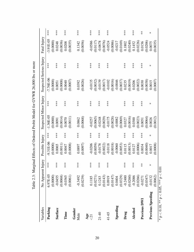
5.4 ANALYSIS OF MARGINAL EFFECTS
The marginal effects show how the probability of each injury severity level changes with a one
unit change in the independent variables. Table 2.3 and Table 2.4 summarize the marginal effect
estimated for the ordered probit model of the two groups. The marginal effects of the dummy
variable, which are calculated differently, are based on the probabilities of different injury levels
when the indicator equals 0 and 1, while all other variables are equal to their means.
14

A one unit increase in the availability of parking spots produces no increase in the injury
outcome with a probability of ”0.007 %”. To decrease the possible injury, suspected minor injury,
suspected major injury and fatal injury outcome probabilities by -0.009%, -0.01%, -0.007%, and
-0.004%, respectively. The marginal effects provide further insight into the correlation between
commercial truck driver injury severity and parking availability. Additional parking spots could
decrease the probability outcome of higher-level injuries and apparently increase the probability of
no injury. The relatively small percentage change is caused by the unit of the independent variable.
For number of total parking, one unit incremental represents one addition parking spot.
With regards to other dummy explanatory variables, when a driver has been involved in a drug-
related offense, the probabilities of injury increase as follows: fatal injury, 18.02 %; serious injury,
2.35%; minor injury, 3.27%; possible injury, 1.15%; and no injury, 24.8%. The marginal effects
indicate that clear surface conditions, night driving, drug and/or alcohol involvement, previous
DWI history, and an older driver can result in particularly severe injuries.
In contrast, the statistical significance of surface conditions, time of the accident, driver gen-
der, and previous speeding violations varies between groups. Similarly, in ordered probit model
analysis, all of the explanatory variables mentioned lose the significance in any level.
5.5 DISCUSSION AND IMPLICATIONS
Overall, the results from this study suggest that more adequate parking spaces, younger drivers,
and stricter enforcement of drug and alcohol policies can reduce the injury severity of commer-
cial drivers during crashes. Environmental factors lose statistical significance when the vehicle’s
GVWR is reduced to the 10,000-26,000 lb range. One explanation for the loss of significance is
that drivers drive more cautiously at night and when weather and surface conditions are poor. Two
principal policy implications follow from our findings. First, the need to invest in adequate com-
mercial parking facilities is urgent. The shortage of commercial vehicle parking spaces increases
the crash rate for commercial vehicles Banerjee et al. (2009). It also raises the probability that
15

commercial vehicle drivers will suffer severe injuries. Second, road monitoring activities at night
should be enhanced.
6. CONCLUSION
This paper addresses a national safety issue related to available truck parking in the United States
and finds a positive relationship between truck accident severity and access to available parking.
Stated differently, improved access and proximity to available parking reduces the severity of truck
accidents. We utilize an ordered probit model to evaluate commercial truck driver injury severity,
utilizing two national databases: 1) truck accident database and 2) truck parking locations. The
estimation results indicate a statistically significant correlation between commercial truck parking
availability and truck driver injury severity. An increase in the total number of parking spots within
a thirty-minute driving distance reduces the probability of a higher degree of injury and increases
the probability of a less severe injury. Several other factors impacting truck accident severity are
specific to the environment and driver characteristics. Adverse surface conditions, night driving,
older drivers, male drivers, and drug or alcohol involvement have a higher probability of a severe
injury.
There are several extensions of this study that would be interesting, given access to available
data. The direction of travel for observations in the truck accident database was not available.
Had this information been available, a more refined evaluation of parking availability ahead of and
past the accident scene could have been considered. In the current study, parking facilities are
calculated based on the longitude and latitude of crash locations and parking facilities. Distances
to these facilities are based on driving times in either direction. In addition, we had no information
related to how long the truck driver had been driving prior to the accident. Currently, truck drivers
must adhere to federal limits on hours of service. But the driving hours of the commercial truck
drivers prior to the crash are not reported but may be available in the future with the electronic log
device mandate. The hours of driving are a key indicator because they affect fatigue/sleepiness.
16

Lastly, factors related to traffic density was not included in the model because of a lack of sufficient
daily truck traffic volume data.
17

Tabl
e2.
1:V
aria
ble
Defi
nitio
nan
dD
escr
iptiv
eSt
atis
tics
GV
WR
10,0
01lb
s-2
6,00
0lb
sG
VW
R26
,000
lbs
orm
ore
Var
iabl
eTi
tleD
escr
iptio
nM
ean
S.D
.M
ean
S.D
.
Dep
ende
ntVa
riab
leIn
jury
Seve
rity
Lev
el0
=no
appa
rent
inju
ry0.
985
1.45
40.
8308
1.34
551
=po
ssib
lein
jury
2=
susp
ecte
dm
inor
inju
ry3
=su
spec
ted
seri
ous
inju
ry4
=fa
tali
njur
yE
xpla
nato
ryVa
riab
lePa
rkin
gN
umbe
roft
otal
park
ing
spot
sw
ithin
30m
inut
esdr
ivin
gdi
stan
ce61
2.11
332.
8557
7.98
348.
19Su
rfac
e1
=dr
y,0
=ot
herw
ise
1.28
370.
8194
1.32
950.
8181
Tim
e1
=N
ight
(22:
00-6
:00)
,0=
othe
rwis
e1.
4238
0.89
931.
5314
0.90
69G
ende
r1
=M
ale,
2=
Fem
ale
0.97
020.
1700
0.97
420.
1585
Age
Age
ofdr
iver
(yea
rs)
40.1
532
13.1
472
44.6
220
11.6
233
Age
Gro
ups
1=
less
than
21,2
=21
-40,
3=
41-6
4,4
=65
and
abov
eSp
eedi
ng1
=Y
es,0
=N
o0.
0556
0.23
570.
2031
0.40
39D
rug
1=
Yes
,0=
No
0.03
330.
1794
0.02
200.
1466
Alc
ohol
1=
Yes
,0=
No
0.02
010.
1405
0.00
970.
0981
Prev
ious
DW
I1
=Y
es,0
=N
o0.
0140
0.16
150.
0072
0.09
28Pr
evio
usSp
eedi
ng1
=Y
es,0
=N
o0.
3021
0.72
320.
3717
0.74
82
No.
ofO
bser
vatio
n1,
142
9,46
2
18

Tabl
e2.
2:O
rder
edPr
obit
Mod
elE
stim
atio
nR
esul
ts
Var
iabl
esG
VW
R26
,000
lbs
orm
ore
GV
WR
10,0
01lb
s-2
6,00
0lb
s
Coe
ffici
ent
Std.
Err
.P
-val
ueC
oeffi
cien
tSt
d.E
rr.
P-v
alue
Park
ing
-1.8
4E-0
40.
0000
0.00
0-2
.21E
-04
0.00
010.
000
Surf
ace
Adv
erse
Con
ditio
n0.
1217
0.01
850.
000
0.06
010.
0521
0.24
9Ti
me
Nig
ht(2
2:00
-6:0
0)0.
0957
0.01
580.
000
0.06
390.
0506
0.20
7G
ende
rM
ale
1.46
350.
2494
0.00
00.
6067
0.71
140.
394
Age
<21
-0.3
352
0.08
400.
000
-0.4
593
0.13
290.
001
21-4
0-0
.333
80.
0392
0.00
0-0
.703
30.
1056
0.00
041
-65
-0.2
416
0.03
850.
000
-0.6
330
0.10
590.
000
Spee
ding
Yes
0.10
880.
0902
0.22
80.
0124
0.19
260.
949
Dru
gY
es0.
6320
0.06
830.
000
0.80
710.
1557
0.00
0A
lcoh
olY
es0.
5299
0.06
810.
000
0.48
580.
1300
0.00
0Pr
evio
usD
WI
Yes
0.07
070.
0897
0.43
00.
6640
0.18
330.
000
Prev
ious
Spee
ding
Yes
0.03
470.
0163
0.03
30.
0621
0.04
850.
200
Thre
shol
dsµ1
1.55
50-
-0.0
606
-µ2
1.85
840.
0000
0.27
640.
0000
µ3
2.18
200.
0000
0.69
120.
0000
µ4
2.35
710.
0000
0.98
200.
0000
No.
ofob
serv
atio
n28
,909
3,37
3Lo
g-lik
elih
ood
-33,
132.
70-4
,559
.16
—B
ase
Cas
e
19
Tabl
e2.
3:M
argi
nalE
ffec
tsof
Ord
ered
Prob
itM
odel
forG
VW
R26
,000
lbs
orm
ore
Var
iabl
esN
oA
ppar
entI
njur
yPo
ssib
leIn
jury
Susp
ecte
dM
inor
Inju
rySu
spec
ted
Seri
ous
Inju
ryFa
talI
njur
y
Park
ing
6.97
E-0
5**
*-9
.31E
-06
***
-1.3
6E-0
5**
*-7
.76E
-06
***
-3.9
1E-0
5**
*(0
.000
0)(0
.000
0)(0
.000
0)(0
.000
0)(0
.000
0)Su
rfac
e-0
.045
5**
*0.
0065
***
0.00
91**
*0.
0051
***
0.02
48**
*(0
.006
8)(0
.001
1)(0
.001
4)(0
.000
8)(0
.003
6)Ti
me
-0.0
365
***
0.00
47**
*0.
0070
***
0.00
40**
*0.
0208
***
(0.0
061)
(0.0
008)
(0.0
011)
(0.0
007)
(0.0
035)
Gen
der
Mal
e-0
.349
2**
*0.
0897
***
0.08
62**
*0.
0392
***
0.13
42**
*(0
.023
9)(0
.009
7)(0
.006
8)(0
.002
6)(0
.005
6)A
ge<
210.
1185
***
-0.0
206
***
-0.0
257
***
-0.0
135
***
-0.0
586
***
(0.0
271)
(0.0
059)
(0.0
065)
(0.0
032)
(0.0
117)
21-4
00.
1243
***
-0.0
178
***
-0.0
248
***
-0.0
139
***
-0.0
678
***
(0.0
143)
(0.0
022)
(0.0
029)
(0.0
017)
(0.0
076)
41-6
50.
0919
***
-0.0
118
***
-0.0
175
***
-0.0
102
***
-0.0
524
***
(0.0
147)
(0.0
018)
(0.0
028)
(0.0
016)
(0.0
086)
Spee
ding
0.04
04-0
.006
0-0
.008
2-0
.004
6-0
.021
7(0
.032
9)(0
.005
3)(0
.006
9)(0
.003
7)(0
.016
9)D
rug
-0.2
480
***
0.01
15**
*0.
0327
***
0.02
35**
*0.
1802
***
(0.0
260)
(0.0
013)
(0.0
016)
(0.0
019)
(0.0
240)
Alc
ohol
-0.2
086
***
0.01
27**
*0.
0300
***
0.02
06**
*0.
1452
***
(0.0
266)
(0.0
006)
(0.0
023)
(0.0
022)
(0.0
226)
Prev
ious
DW
I-0
.027
1**
0.00
34**
*0.
0051
***
0.00
30**
*0.
0156
**(0
.034
7)(0
.004
0)(0
.006
4)(0
.003
8)(0
.020
6)Pr
evio
usSp
eedi
ng-0
.013
2*
0.00
17*
0.00
26*
0.00
15*
0.00
75*
(0.0
062)
(0.0
008)
(0.0
012)
(0.0
007)
(0.0
035)
*p<
0.10
,**
p<
0.05
,***
p<
0.01
20

Tabl
e2.
4:M
argi
nalE
ffec
tsof
Ord
ered
Prob
itM
odel
forG
VW
R10
,001
lbs
-26,
000
lbs
Var
iabl
esN
oA
ppar
entI
njur
yPo
ssib
leIn
jury
Susp
ecte
dM
inor
Inju
rySu
spec
ted
Seri
ous
Inju
ryFa
talI
njur
y
Park
ing
8.82
E-0
5**
*-4
.69E
-06
***
-1.6
7E-0
5**
*-1
.53E
-05
***
-5.1
6E-0
5**
*(0
.000
0)(0
.000
0)(0
.000
0)(0
.000
0)(0
.000
0)Su
rfac
e-0
.024
00.
0014
0.00
470.
0042
0.01
37(0
.020
8)(0
.001
4)(0
.004
1)(0
.003
6)(0
.011
7)Ti
me
-0.0
255
0.00
120.
0047
0.00
440.
0152
(0.0
202)
(0.0
008)
(0.0
036)
(0.0
035)
(0.0
123)
Gen
der
Mal
e-0
.229
50.
0313
0.05
590.
0402
0.10
21(0
.240
7)(0
.052
5)(0
.069
0)(0
.041
0)(0
.078
4)A
ge<
210.
1781
***
-0.0
205
***
-0.0
413
***
-0.0
313
***
-0.0
850
***
(0.0
486)
(0.0
086)
(0.0
131)
(0.0
087)
(0.0
188)
21-4
00.
2749
***
-0.0
141
***
-0.0
503
***
-0.0
464
***
-0.1
641
***
(0.0
396)
(0.0
026)
(0.0
073)
(0.0
070)
(0.0
249)
41-6
50.
2481
***
-0.0
169
***
-0.0
489
***
-0.0
426
***
-0.1
398
***
(0.0
400)
(0.0
037)
(0.0
084)
(0.0
072)
(0.0
224)
Spee
ding
0.00
49-0
.000
3-0
.000
9-0
.000
9-0
.002
9(0
.076
8)(0
.004
4)(0
.014
8)(0
.013
3)(0
.044
3)D
rug
-0.2
909
***
-0.0
220
***
0.01
76**
*0.
0380
***
0.25
73**
*(0
.045
4)(0
.010
7)(0
.006
5)(0
.003
4)(0
.060
0)A
lcoh
ol-0
.186
7**
*-0
.004
3**
*0.
0224
***
0.02
89**
*0.
1397
***
(0.0
464)
(0.0
051)
(0.0
024)
(0.0
061)
(0.0
440)
Prev
ious
DW
I-0
.246
8**
*-0
.013
4**
*0.
0213
***
0.03
51**
*0.
2038
***
(0.0
589)
(0.0
106)
(0.0
040)
(0.0
055)
(0.0
678)
Prev
ious
Spee
ding
-0.0
248
0.00
120.
0046
0.00
430.
0148
(0.0
193)
(0.0
008)
(0.0
035)
(0.0
033)
(0.0
117)
*p<
0.10
,**
p<
0.05
,***
p<
0.01
21

CHAPTER THREE:
ESTIMATING THE EFFECT OF RETAIL ELECTRICITY MARKET
RESTRUCTURING:A SYNTHETIC CONTROL APPROACH
1. INTRODUCTION
Starting from late 1990s, a movement to restructure electricity market swept through around half
of the US states. Two decades after initiation of electricity market restructuring, sixteen states still
actively engaged in deregulating retail electricity market, while six states suspended the dereg-
ulation process. The debate of whether the introduction of competition into electricity industry
improves efficiency never end.
The electricity supply industry includes generation, transmission, distribution and retail. Re-
structuring of retail services involves the adoption of retail competition to provide more freedom
of choice to end-use customers. Kwoka (2008) has reviewed many of the electricity market dereg-
ulation studies to determine the impact of restructuring on average prices. The general approach of
most studies is to identify a given set of states as “restructured” and to compare the growth of prices
within these states to those states still under regulation. The author summarizes the results from
these studies are mixed with both positive and negative effects on price, although more studies find
lower prices in restructured states than those not.
Su (2015) focuses on the availability of retail choice utilizing two measures: traditional cost-
of-service (COS) regulation and share of total revenues earned by retail power marketers. A
difference-in-difference approach is applied to estimate the policy impact for U.S. states that re-
structured their retail electricity market. Results suggest the significantly lower prices affected
by restructuring is observed for a short period for residential customers but not commercial or
industrial customers.
The impact on retail customer prices could also result from upstream changes relating to the re-
structuring in generation, transmission, and distribution. Joskow (2006) analyzes state-level panel
22

data on key cost factors, such as fuel prices, contracts, share of hydro and nuclear generation. The
restructuring treatments are examined by two dummy variables: the year retail competition was in-
troduced, and the share of energy generated from unregulated generators in the state. He concludes
the residential and industrial electricity prices both fall with deregulation in electricity generation
and retail competition.
Borenstein and Bushnell (2015) build a model to examine annual retail residential electricity
price changes from 1997 to 2012. They conclude that once gas price is controlled for restructuring
in generation has no significant effect on retail price. Their hypothesis retail prices in restructured
states during the period 2006 -2008 are affected by the fall of natural gas prices and rate freezes for
protection of generates mainly still under regulation. They argue in the paper it is not appropriate
to claim restructuring a failure or a success since results depend on change in exogenous input
costs.
The question of efficiency in deregulated electricity markets is attracting more attention. While
many neoclassical economists conclude deregulation works. Events like the California power crisis
of 2000 and 2001 weaken confidence in the ability of deregulated electricity markets to efficiently
allocate electricity. Opposition to deregulation in electricity markets is particularly strong. For
instance, market manipulation was considered the main reason for failure in restructuring the elec-
tricity market. Van Doren and Taylor (2004) suggest vertical integration may be the most efficient
organizational structure for the electricity industry.
Evidence of restructured market inefficiency has been shown in California (Borenstein et al.
2002, and Joskow and Kahn 2001), Pennsylvania-New Jersey-Maryland (PJM) (Pirrong and Jer-
makyan 1999, and Longstaff and Wang 2004), New York (Saravia 2003, and Hadsell and Shawky
2007) and Europe Graf and Wozabal (2013). Three major measurements have been used to mea-
sure market efficiency: 1) by comparing realized price to competitive benchmarks;2) as the differ-
ence between Day Ahead (DA) and Real Time (RT) prices; and 3) time-varying characteristics of
price volatility.
23

Market power is measured by comparing realized prices to competitive benchmarks. A number
of empirical studies have concluded that sellers have exercised significant market power in Cali-
fornia’s wholesale electricity market (Borenstein et al. 2002, Wolak et al. 2000,and Joskow and
Kahn 2001). Borenstein and Bushnell (1999) simulated the market using a Cournot model. Even
with an assumed demand elasticity of -0.1, which is larger than any estimate under the California
transition plan, they found very significant markups without any collusion.
Another line of research examines the Day Ahead (DA) market with Real Time (Spot) mar-
ket. The convergence of DA and spot price could improve the efficiency of resource allocation
and reduce start-up cost. Several studies find significant nonzero DA premiums (DA price mi-
nus RT price) for PJM (Pirrong and Jermakyan 1999, and Longstaff and Wang 2004), California
Borenstein and Bushnell (1999), and New York Hadsell and Shawky (2007).
Time-varying characteristics of price volatility is another measurement of retail electricity mar-
ket efficiency. Analysis like this improves the determination of the informational efficiency for
these markets, such as how quickly traders react to changing market conditions. Some articles
compare different duration of the shocks within DA and spot markets. Hadsell and Shawky (2007),
for example, find the shocks persist longer in DA markets than in the spot market for heavily con-
gested areas.
This paper aims to identify the impacts on residential electricity price of retail electricity market
restructuring in the United States. Average treatment effect was examined by applying a synthetic
control method that is integrated with generalized linear models. Control variables are included
in the model to adjust for factors that violate the parallel trend assumption. Deregulated states are
grouped and analyzed into 5 Regional Transmission Organizations (RTO) including Independent
System Operator New England (ISO-NE), Midcontinent Independent System Operator (MISO),
New York Independent System Operator (NYISO), PJM Interconnection (PJM), Electric Reliabil-
ity Council of Texas (ERCOT). Oregon state is analyzed separately.
Our main finding of the impacts varies by location and structure of electricity market restructur-
24

ing. ISO-NE, MISO, NYISO, and PJM all show significant decrease of retail residential electricity
price compared to the synthetic group, while ERCOT indicates a relatively higher price. The treat-
ment effect analysis does not highlight any change of price for Oregon state.
This paper is the first application of synthetic control method analyzing the impact of retail
electricity market restructuring. The different results within RTOs reveal different approach with
electricity market restructuring which is important to both policy makers and researchers.
The remainder of the paper is organized as follows. Data source and formation of synthetic
groups are summarized in Section 2. Section 3 presents the explanation of Difference-in-difference
method and Synthetic Control Method (SCM) applied in this research. Section 4 summarizes the
results and discusses the possible implications of the findings for policy. Section 5 concludes the
main findings and contribution of this research.
2. DATA
2.1 DEPENDENT VARIABLE
The data and information utilized in this study are obtained from U.S. Energy Information Admin-
istration website for average retail price of electricity by end-user sectors and state from 1990 to
2014. Nominal price is deflated with annual CPI for each state to calculate the real price. Unit for
residential retail electricity price is cents per KWh.
2.2 EXPLANTORY VARIABLES
To control for other factors that affect the retail electricity price, the following control variables
were added to the model for a more robust result including coal price, natural gas price, number of
total generation plants, emission of CO2, and number of retail customers.
The coal and natural gas price are annual data collected from U.S. EIA website by end-use
sectors and state from 1970 to 2013. These two independent variables are considered as part of the
25

fuel cost which are the key factors that influence the price of electricity.
The number of total generation plants data are collected only for the annual total summation.
We aggregate the generation facility by all fuel sources which includes coal, petroleum, natural
gas, wood, wind, hydroelectric and nuclear.
Number of retail customers are used as the third independent variable which are summarized
by state and by end-user sectors. The period availability for the data is also from 1990-2014. Both
dependent and explanatory variables are summarized in Table 3.1.
2.3 GROUPS AND PERIODS SELECTION FOR SCM
The creation and expansion of Regional Transmission Organizations (RTOs) and Independent Sys-
tem Operators (ISO) coincided with the rapid adoption of retail electricity market restructuring in
late 1990s. By 2014, two thirds of the power control areas in the U.S. are covered by RTOs (See
Figure 3.1 ). RTOs/ISOs are designed for providing non-discriminatory access to transmission.
This study coverts state level data to RSOs/ISOs in regions by weighted average. Deregulated
states are grouped and analyzed into five RTOs/ISOs, including Independ System Operator New
England (ISO-NE), Midcontinent Independent System Operator (MISO), New York Independent
System Operator (NYISO), PJM Interconnection (PJM), Electric Reliability Council of Texas (ER-
COT). All state data under restructuring are replaced by their local RTO/ISOs. The only exception
is Oregon state. Since the absence of any regional transmission organization around Oregon, this
state is analyzed separately as an individual state.
Restructuring in retail electricity market is a procedure starting with legislative activities to
revise state law, following with policy implementation to create free choice from alternative sup-
pliers for retail electricity customer . In this study, the year of policy implement after the treatment
year since the electricity price is violated only after the creation of the competition.
26
3. METHODOLOGY
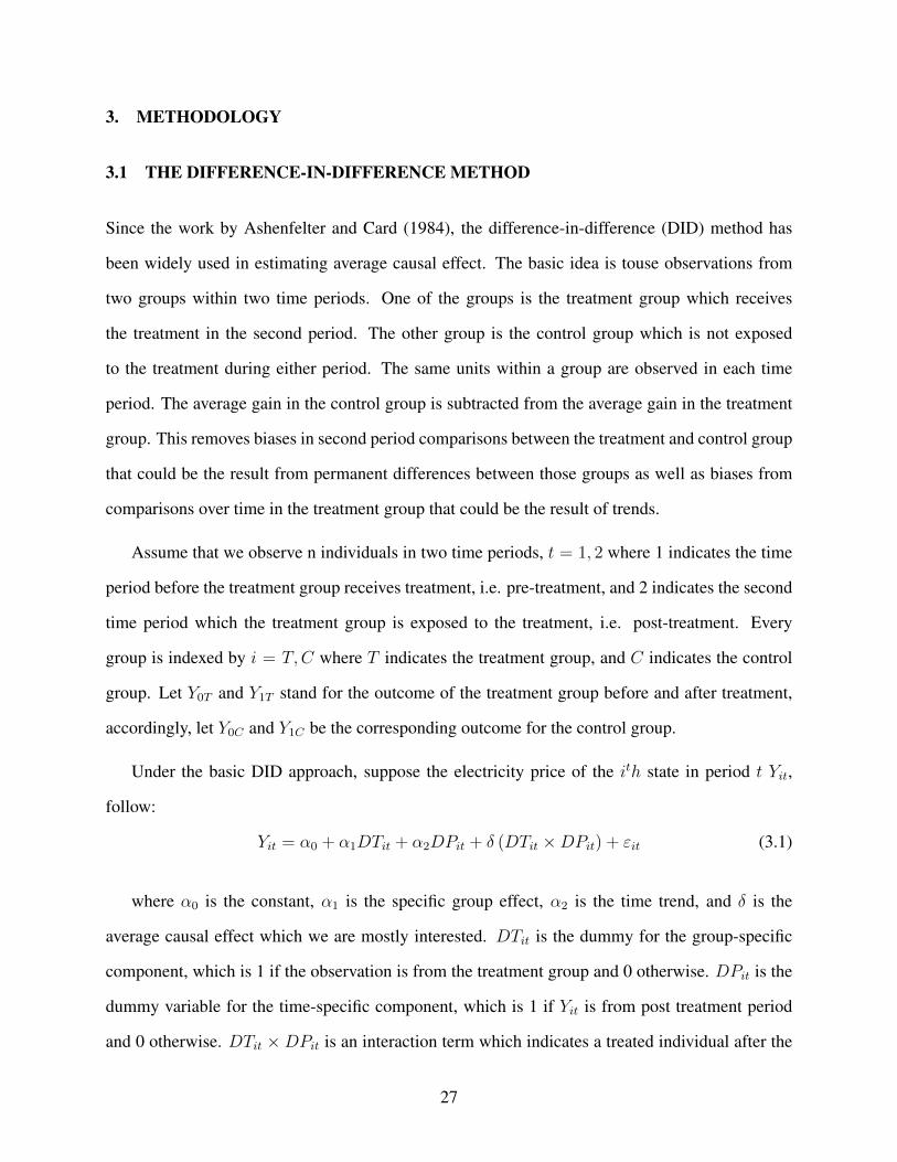
3.1 THE DIFFERENCE-IN-DIFFERENCE METHOD
Since the work by Ashenfelter and Card (1984), the difference-in-difference (DID) method has
been widely used in estimating average causal effect. The basic idea is touse observations from
two groups within two time periods. One of the groups is the treatment group which receives
the treatment in the second period. The other group is the control group which is not exposed
to the treatment during either period. The same units within a group are observed in each time
period. The average gain in the control group is subtracted from the average gain in the treatment
group. This removes biases in second period comparisons between the treatment and control group
that could be the result from permanent differences between those groups as well as biases from
comparisons over time in the treatment group that could be the result of trends.
Assume that we observe n individuals in two time periods, t = 1, 2 where 1 indicates the time
period before the treatment group receives treatment, i.e. pre-treatment, and 2 indicates the second
time period which the treatment group is exposed to the treatment, i.e. post-treatment. Every
group is indexed by i = T,C where T indicates the treatment group, and C indicates the control
group. Let Y0T and Y1T stand for the outcome of the treatment group before and after treatment,
accordingly, let Y0C and Y1C be the corresponding outcome for the control group.
Under the basic DID approach, suppose the electricity price of the ith state in period t Yit,
follow:
Yit = α0 + α1DTit + α2DPit + δ (DTit ×DPit) + εit (3.1)
where α0 is the constant, α1 is the specific group effect, α2 is the time trend, and δ is the
average causal effect which we are mostly interested. DTit is the dummy for the group-specific
component, which is 1 if the observation is from the treatment group and 0 otherwise. DPit is the
dummy variable for the time-specific component, which is 1 if Yit is from post treatment period
and 0 otherwise. DTit ×DPit is an interaction term which indicates a treated individual after the
27
intervention.
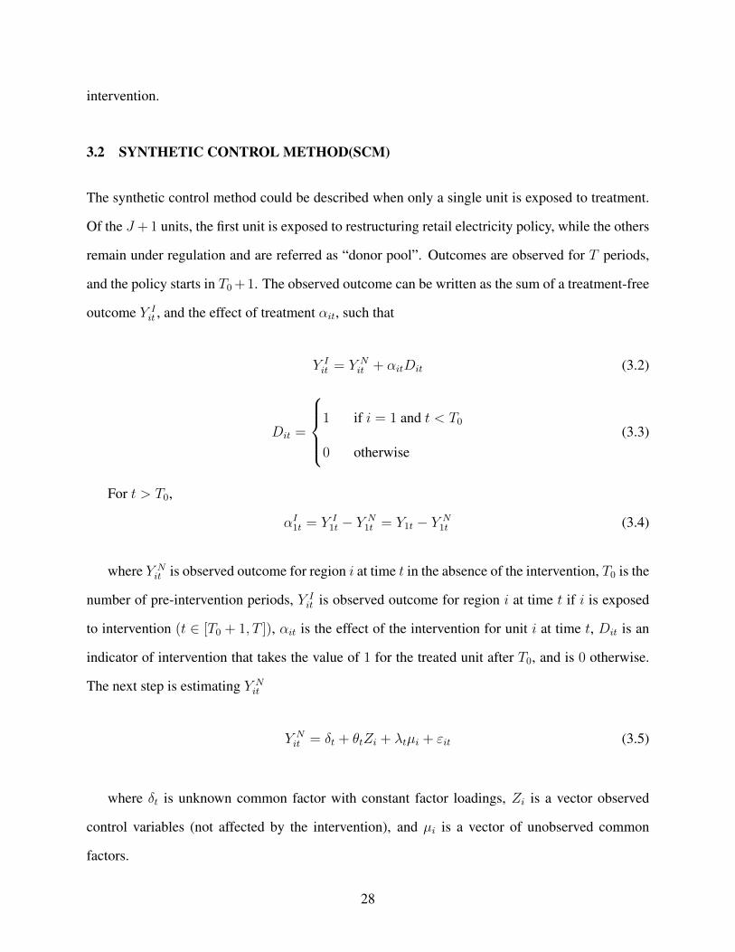
3.2 SYNTHETIC CONTROL METHOD(SCM)
The synthetic control method could be described when only a single unit is exposed to treatment.
Of the J + 1 units, the first unit is exposed to restructuring retail electricity policy, while the others
remain under regulation and are referred as “donor pool”. Outcomes are observed for T periods,
and the policy starts in T0 + 1. The observed outcome can be written as the sum of a treatment-free
outcome Y Iit , and the effect of treatment αit, such that
Y Iit = Y N
it + αitDit (3.2)
Dit =
1 if i = 1 and t < T0
0 otherwise(3.3)
For t > T0,
αI1t = Y I
1t − Y N1t = Y1t − Y N
1t (3.4)
where Y Nit is observed outcome for region i at time t in the absence of the intervention, T0 is the
number of pre-intervention periods, Y Iit is observed outcome for region i at time t if i is exposed
to intervention (t ∈ [T0 + 1, T ]), αit is the effect of the intervention for unit i at time t, Dit is an
indicator of intervention that takes the value of 1 for the treated unit after T0, and is 0 otherwise.
The next step is estimating Y Nit
Y Nit = δt + θtZi + λtµi + εit (3.5)
where δt is unknown common factor with constant factor loadings, Zi is a vector observed
control variables (not affected by the intervention), and µi is a vector of unobserved common
factors.
28

Suppose there exists a set of weights(ω∗2, · · · , ω∗J+1
)satisfying
∑J+1j=2 ω
∗j = 1 such that
J+1∑j=2
ω∗jYj1 = Y1,1
...J+1∑j=2
ω∗jYjT0 = Y1,T0
J+1∑j=2
ω∗jZj = Z1 (3.6)
The treatment effect estimator
α1t = Y1t −J+1∑j=2
ω∗jYit for t ∈ {T0 + 1, · · · , T} (3.7)
Define a linear combination of pre-intervention outcomes as:
YK
i =
T0∑s=1
ksYis (3.8)
Consider M of such linear combination defined as vectors K1, . . . , KM , and
Let X1 =(Z ′1, Y
K1
1 , · · · , Y KM
1
)(3.9)
where a (k × 1) vector of pre-intervention characteristics for the Treated Unit
Let X0 =(Z ′j, Y
K1
j , · · · , Y KM
j
)(3.10)
where a (k × J) vector of pre-intervention characteristics for the Unaffected Regions
29

W ∗ is chosen by solving:
minW
√(X1 −X0W )′V (X1 −X0W ) (3.11)
s.t. w2 + · · ·+ wJ+1 = 1 (3.12)
w2 ≥ 0, · · · , wJ+1 ≥ 0 (3.13)
V is a k × k positive definite and diagonal matrix, which assigns weights according to the
relative importance of the covariates and the pre-intervention outcomes. A joint optimal choice of
V and W minimize the mean square error of the estimator Abdel-Aty (2003).
3.3 ASSUMPTION
The difference-in-difference method requires a parallel trend assumption, which is critical in the
estimation. The treatment group and control group will follow the same trend over time in the
absence of the treatment.
E [Y ′2T − Y ′1T ] = E [Y2C − Y1C ] (3.14)
where Y ′it represents outcomes of the treatment group not exposed to treatment.
However, the difference between the treatment and control groups are not only caused by the
effect. We need find a set of control variables Xi to adjust the possible violation of the parallel
trend assumption Abdel-Aty (2003), which forms the following equation
Yit = α0 + α1DTit + α2DPit + δ (DTit ×DPit) + βXit + µi + εit (3.15)
where β is a vector of the coefficients for control variables. Xi contains all the control variables
that affect Yit and are uncorrelated with εit. The above assumption is still assumed to hold, but now
30

is conditional on covariates X:
E [Y ′2T − Y ′1T | Xi, µi] = E [Y2C − Y1C | Xi, µi] (3.16)
Then the assumption is extended for the synthetic control method by assuming that the condi-
tioning set now is a realization of {y1,t, · · · , yJ+1,t} for t = 1, · · · , T conditional on D (1, T0) = 1.
We also assume the treatment assignment is not informative about the first moment of the transitory
shocks.
E (εit | Di, λi, xi) = E (εit | λi, xi) = 0 (3.17)
We do not assume that (λi, xi) and Di are uncorrelated and selection into treatment can freely
depend on observed and unobserved heterogeneity terms.
4. RESULTS
In this section, we construct synthetic control regions that best reproduces the values of the predic-
tors for each outcome variable of interest in the pre-intervention periods. We estimate the effect
of retail electricity restructuring on the outcome variables as the difference between each outcome
variable in each treated region and its synthetic versions in the year of the intervention. Control
variables like natural gas price, coal price, emission of local CO2, real GDP, number of generation
facilities, and count of residential retail customers are added to the estimation for eliminating other
factors affecting retail electricity price.
4.1 RESIDENTIAL RETAIL PRICE
We look at the residential retail price for the treated regions at first. This will give us a better un-
derstanding of what happened when the treated regions where exposed to electricity restructuring
in the residential retail market. Figure 3.2 presents the results for the treated regions (ISO-NE,
31

PJM, MISO, NYISO, ERCOT, Oregon).
From the graphs we could clearly see the synthetic controls closely match the treated regions
in the pre-intervention period. For ISO-NE, PJM, MISO and NYISO, the residential retail price
could be seen clearly in the graph in the treated regions are lower than the synthetic counterparts.
With the intervention of the restructuring in the residential retail electricity market, the introduc-
tion of competition successfully achieves the original goal of lowering retail price and sufficiently
allocating resources.
For ERCOT in Texas, the residential retail price in the treated region is greater than the syn-
thetic counterpart. The result indicates a negative effect of the intervention on retail electricity
market throughout the post-intervention period. The actual electricity price of retail residential
customers is higher than the synthetic estimation. From the price perspective, the increase of the
price is a sign of failure or inefficiency for electricity restructuring occurred in Texas on 2002.
For Oregon state, we find no effect on residential retail price after the intervention of electricity
restructuring since 1997. The actual residential electricity price coincided with synthetic counter-
parts closely in both the pre-intervention and post-intervention periods. Compared to the results
for other RSOs/ISOs, we could not conclude any successfully intervention from retail electricity
market restructuring happened in Oregon.
4.2 COMMERCIAL RETAIL PRICE
In Figure 3.3, we present findings regarding commercial retail price outcomes for all treated
ISOs/RTOs. Similar to the previous finds in residential retail markets, we could still find a sig-
nificant lower price for ISO-NE, PJM, MISO and NYISO continuously. This result indicates the
restructuring in retail markets also affect commercial retail price negatively. Reduction of the ac-
tual price proves the efficient policy changed with the introduction of more competition within
the commercial end-user market. The commercial users are also benefited from retail electricity
market restructuring.
32

Results in ERCOT are reasonably similar to residential retail price as well. The treated units
indicate a higher commercial retail price than synthetic estimation price. The result still shows
positive effect on commercial retail price with policy intervention. The only exception happens
after 2010; price in treated region turns lower than the actual price. Restructuring in the retail
electricity market still shows no apparent effect on commercial price in Oregon state.
4.3 INDUSTRIAL RETAIL PRICE
Finally, we study the effects on industrial retail prices for retail electricity market restructuring. We
present findings in figure 3.4 for all RTOs/ISOs in industrial retail price. For ISO-NE and PJM, the
pre-intervention period is very similar between threated regions and their corresponding synthetic
controls. In the post-intervention period, the actual price outcomes in the treated regions are lower
than synthetic counterparts. However, for MISO and NYISO, the synthetic controls do not closely
match the treated regions in the pre-intervention period, which leads an inconsistent relationship
between the actual industrial retail price trend and synthetic control estimation trend.
For ERCOT, the estimation proves same outcomes as in the residential and commercial market.
This result illustrates the restructuring in Texas clearly: it did not cause a decrease in the retail
electricity price for residential, commercial and industrial markets. The policy intervention on
industrial retail market did not effect Oregon state as well. The gaps between actual price and
synthetic estimation price are relatively small compared to other RSOs/ISOs.
5. CONCLUSION
In the late 1990s, some of the U.S. states began the process of restructuring in the electricity
industry. The mix of results led by the deregulation and regulatory reform in the past two decades
is attracting more attention. Our analysis agrees with the mixed results as other research Bushnell
et al. (2017). This paper is the first application of synthetic control method in state-level panel data
to estimate the policy impact on retail electricity price for residential, commercial, and industrial
33

customers. Besides Oregon state, we could find a significant impact on all other ISOs/RTOs. The
direction of the intervention is not consistent for all the regions. However, the mixed results could
lead to a deeper analysis for the variety in retail electricity market restructuring within regions as
a better understanding of the practice of the policy in the last twenty years.
Our study finds the effects of residential retail electricity market restructuring vary by geo-
graphical locations. In our analysis of intermediate factors, we find robust evidence that the inter-
vention caused a residential retail price drop in ISO-NE, PJM, MISO and NYISO. This suggests
that the market restructuring actively provides the residential end-customers freedom of choice
for utility service providers. The competition leads a lower retail price at the market equilibrium
than natural monopoly market price marked in regions not utilizing restructuring. However, the
policy intervention shows only positive effects for residential retail price in ERCOT, while there is
evidence for the effect in Oregon state electricity market deregulation.
The regression results suggest that the electricity price is significantly affected by the event
of deregulation. But the signs are inconsistent within the groups. The positive effect can be in-
terpreted as the inefficiency of the electricity market restructure, which might be related to the
increasing market power of the generator and distributor. The negative sign could prove the effi-
ciency of the deregulation process.
Each state applied a different electricity market restructuring plan. The difference in the im-
pacts of deregulation, more detailed comparisons between different states as a key to the reason
why the efficiency of deregulation differs by states.
34
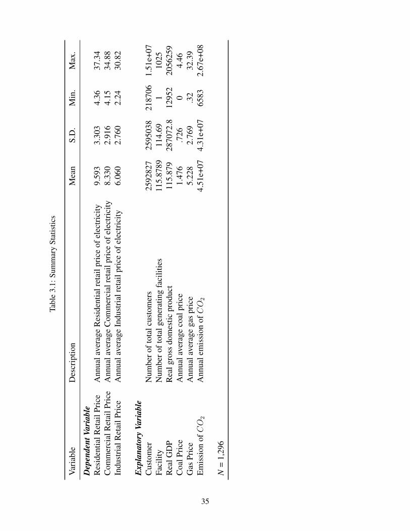
Tabl
e3.
1:Su
mm
ary
Stat
istic
s
Var
iabl
eD
escr
iptio
nM
ean
S.D
.M
in.
Max
.
Dep
ende
ntVa
riab
leR
esid
entia
lRet
ailP
rice
Ann
uala
vera
geR
esid
entia
lret
ailp
rice
ofel
ectr
icity
9.59
33.
303
4.36
37.3
4C
omm
erci
alR
etai
lPri
ceA
nnua
lave
rage
Com
mer
cial
reta
ilpr
ice
ofel
ectr
icity
8.33
02.
916
4.15
34.8
8In
dust
rial
Ret
ailP
rice
Ann
uala
vera
geIn
dust
rial
reta
ilpr
ice
ofel
ectr
icity
6.06
02.
760
2.24
30.8
2
Exp
lana
tory
Vari
able
Cus
tom
erN
umbe
roft
otal
cust
omer
s25
9282
725
9503
821
8706
1.51
e+07
Faci
lity
Num
bero
ftot
alge
nera
ting
faci
litie
s11
5.87
8911
4.69
110
25R
ealG
DP
Rea
lgro
ssdo
mes
ticpr
oduc
t11
5.87
928
7072
.812
952
2056
259
Coa
lPri
ceA
nnua
lave
rage
coal
pric
e1.
476
.726
04.
46G
asPr
ice
Ann
uala
vera
gega
spr
ice
5.22
82.
769
.32
32.3
9E
mis
sion
ofCO
2A
nnua
lem
issi
onofCO
24.
51e+
074.
31e+
0765
832.
67e+
08
N=
1,29
6
35

Figu
re3.
1:M
apof
U.S
.Reg
iona
lTra
nsm
issi
onO
rgan
izat
ions
36

(a)I
SON
E(b
)PJM
(c)N
YIS
O
(d)M
ISO
(e)E
RC
OT
(f)O
rego
n
Figu
re3.
2:E
ffec
tson
Res
iden
tialR
etai
lPri
cefo
rres
truc
ture
dR
SOs/
ISO
s
37
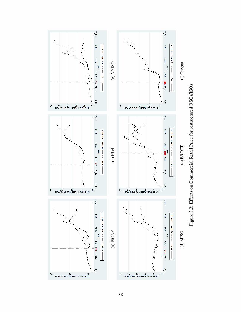
(a)I
SON
E(b
)PJM
(c)N
YIS
O
(d)M
ISO
(e)E
RC
OT
(f)O
rego
n
Figu
re3.
3:E
ffec
tson
Com
mer
cial
Ret
ailP
rice
forr
estr
uctu
red
RSO
s/IS
Os
38
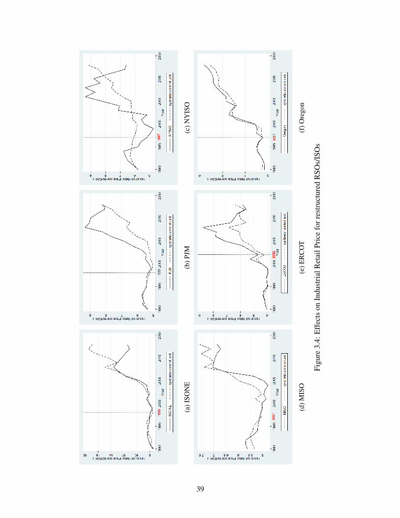
(a)I
SON
E(b
)PJM
(c)N
YIS
O
(d)M
ISO
(e)E
RC
OT
(f)O
rego
n
Figu
re3.
4:E
ffec
tson
Indu
stri
alR
etai
lPri
cefo
rres
truc
ture
dR
SOs/
ISO
s
39

CHAPTER FOUR:
THE EFFECTS OF SUPPLIER DIVERSIFICATION ON FIRM’S FINANCIAL
PERFORMANCE
1. INTRODUCTION
The idea of supplier diversification in managing supply chain partnerships for competitive advan-
tage is of broad interest. Maintaining a supply base with multiple suppliers is adapted by numerous
companies in an effort to deal with supply risks. Traditionally, successful matching between sup-
pliers and customers is based upon matching the needs of the market with the capabilities of the
firm. Now, however, competitive advantage is unlikely to be achieved in that way with the tremen-
dous expansion of information and the breakdown of technology barriers.
A diversification strategy is employed by many customer firms to mitigate supply risk, such
as ordering from multiple suppliers to hedge the risk of random supply shocks within individual
supplier operations. Another benefit of diversification is increased competition as customer firms
are able to choose the supplier with the lowest bid for the same quality. Wu and Choi (2005)
analyze how the customer firms get involved in relationships among suppliers by utilizing the case
study method. Their result indicates the two major goals for the buyer are: 1) managing supply
risk as well as, 2) reducing cost through competition.
This paper studies the relationship between supplier diversification and customer firms’ finan-
cial performance in the manufacturing sector. The diversification of supplier companies is captured
by the number of suppliers and market shares of suppliers with related customer firms. Short-term
and long-term impacts are also examined in our research.
The remainder of this article is structured as follows. In Section 2, we review the current
literature relevant to our research topics in different streams. In Section 3, we describe how the
data is dependent and utilized including information in our model formation. The models and
methodology are explained in Section 4. Section 5 summarizes and discusses regression results
40

for all models. A conclusion for this research is in Section 6.
2. LITERATURE
Three broad streams of research are summarized in this section. The first focuses on understanding
the general supplier-customer relationships within supply chain management. The second line of
research is focused on understanding how the competition within suppliers affects customer firm’s
financial performance. The third area of research discusses on the effects of financial distress and
supplier default risk, and choice between short-term and long-term contract with the suppliers to
counteract the risk.
There are numerous research studies focused on multi-sourcing in supply disruptions manage-
ment, including(Tomlin and Wang 2005, Babich et al. 2007,Babich 2010, and Dada et al. 2007).
However, the external competition among suppliers is not captured by the majority of this research.
Yang et al. (2012) consider a more general model of competition which allows that the manufac-
turer (“customer”) has a dual-sourcing option if it has two suppliers in the supply base. They
conclude the benefits from supplier diversification are a reduction of informational rent payments
to suppliers and competition benefits from asymmetric information for the supplier.
Customer and supplier firms’ financial performance are tightly bonded together with economic
characteristics along the supply chain. A shock to the informational environment or performance
of one firm has an impact on its economically-linked customers or suppliers. Pandit et al. (2011)
examine how supplier firm stock performance response to customer firm earnings news. Likewise,
Cohen et al. (2008) find that supplier stock price responds to changes in customer stock price. At
the industry level, Menzly and Ozbas (2010) find that customer industry returns predict returns of
supplier industries.
A number of studies have examined the linkages between supplier-customer relationships and
economic performance. Johnston et al. (2004) indicates the gains to the customer from successful
relationships in terms of financial and lead time performance. In addition, these relationships can
41

result in improved responsiveness, and customer loyalty (Martin and Grbac (2003)), innovation
(Corsten and Felde 2005, and Johnston et al. 2004), and quality (Johnston et al. (2004)).
According to the finance literature, supplier firm performance is especially vulnerable to de-
creases in demand from customers. Suppliers are susceptible to distress when there is a reduction
in customer firm health. Hertzel et al. (2008) find a decrease in supplier firm value when one of
the customer firms files for bankruptcy. Lian (2017) finds that a supplier is more likely to become
financially distressed if one of its principal customers becomes distressed. The spill-over effects of
poor performance are especially high if the supplier has a concentrated customer base Irvine et al.
(2015).
Attentive market participants recognize the value of information within the supply chain. Guan
et al. (2015) find that financial analysts are more accurate in their supplier forecasts if they cover
both customer- and supplier- linked firms rather than if they follow only the supplier firm. Also,
institutional investors who pay attention to customer firm stock gain from trading in supplier firm
stock Alldredge and Puckett (2016). Moreover, attentive supplier executives incorporate recent
customer earnings news and customer stock returns in their profitable insider trades according to
Alldredge and Cicero (2015).
Another line of research focuses on the competition between suppliers. Wu and Choi (2005)
examine the procurement problem with option contracts in a setting consisting of a single buyer
and n competing sellers. A multi-attribute competition model specializing in electricity market is
also examined by Martınez-de Albeniz and Simchi-Levi (2006). Fu et al. (2010) utilize a portfolio
approach to study the negotiation procedure between one customer firm and n competing suppliers.
The above literatures all assume the supplier and customer hold symmetric information about the
market and competitors.
Some researchers examine the difference between a short-term contract with a supplier and a
long-term partnership. In much of the literature, long-term contracts refer to those signed prior to
the realization of some random variable while short-term contracts refer to those signed after the
42

realization of a stochastic event in a single period. Li and Debo (2009) analyze a model quanti-
fying the value of commitment to a single firm in a two-period contract in which suppliers have
private information about their production costs. They find that a long-term contract increases the
aggressiveness of supplier bidding and helps to oppose the effect of information asymmetry. Klein-
dorfer and Wu (2003) construct and implement a survey comparing long and short-term contracts
under cost uncertainty. Some research about long-term collaborative relationships suggests the
customer tend to prefer closer relationships when they wish to control the dependability of supply
or influence supplier quality and delivery schedules Ellram (1995).
Babich et al. (2007) posit a model with multiple suppliers and a single customer. They con-
sider the default risk from the supplier as exogenous where the suppliers act as Stackbelber leaders
(whichever moves first and then the follower firms move sequentially) in setting the wholesale price
for the downstream customers. Swinney and Netessine (2009) expand the method by considering
the default risk as endogenous and the bargaining power lies with the customer firm. Further-
more, their model also considers the effect over several periods beyond the single period model of
Babich’s research.
Empirical studies are not commonly applied in supply chain management research, especially
under supplier diversification. This paper is the first application of actual supplier’s percentage of
sale data to analyze the relationship between supplier diversification and customer firms’ financial
performance.
3. DATA
3.1 SAMPLE CONSTRUCTION
Due to the data availability, we study the firm’s financial performance from 1985 to 2014. The
information of firm’s returns and other characteristics is obtained from the Mergent Bond Record
database which reports from Standard and Poor, Moody, and Fitch. Our sample is restricted to the
43

customer-supplier relationship data available in Compustat Customer Segments database. Accord-
ing to the statement of Financial Accounting Standards (SFAS) No. 14 and No. 131, all public
companies are required to report information about their major customers that accounts for at least
10% of the total sales and are permitted to optionally disclose information about important cus-
tomers that account for less than 10% of the total sales. Following the approach of Fee and Thomas
(2004), we identify suppliers and customers of the firms. The customer-supplier relationship in-
formation is collected from the Compustat Customer Segments database required hand matching
customer names to the company names found in Compustat. In an effort to be conservative in
the matching of customer names, we are careful to compare names to company websites and the
Business Week company profiles and exclude any questionable matches.
3.2 DEPENDENT VARIABLE
The firm’s financial performance information, such as stock returns, shares outstanding, etc., is
obtained from the Center for Research in Security Prices (CRSP). Only common stocks (with
CRSP shares code 10 and 11) are utilized in the analysis. The firm’s financial statement data is
collected from Compustat Annual. In particular, we focus on the fundamental information that
we will use in the later regression analysis including Dow Jones Industrial Average and net share
issues.
3.3 EXPLANATORY VARIABLE
To control for other factors that affect the customer firms’ return, we include the Dow Jones In-
dustrial Average (DJIA) as a control variable. The data is collected from Yahoo Finance as daily
obserbations data between Jan 1st, 1985 and December 31st, 2016. The index return is calcu-
lated by applying the adjusted closing price for last trading day in each year as annual data. Net
Share Issues (NSI)are calculated at the end of each year as the log of change in the firm’s shares
outstanding over the previous twelve months. The risk free rate is utilized as 10-year treasury
44

constant maturity rate which is collected from Federal Reserve Bank of St. Louis data site.
The firm-level equity and accounting information is obtained from Center for Research in Se-
curity Prices (CRSP) and Compustat, respectively. Our initial sample includes common stocks
listing on the NYSE, Nasdaq, and Amex from January 1978 to December 2016. We focus our
research in manufacturing (SIC codes between 2000 and 3999). We exclude penny stocks with
price under $5.
Both dependent and explanatory variables are summarized in Table 4.1.
4. EMPIRICAL REGRESSION AND RESULTS
4.1 SUPPLIER DIVERSIFICATION ESTIMATION
The objective of our first estimation is identifying the effect of supplier diversification on firm’s fi-
nancial performance for the same year. The identification relies on exhaustive control of confound-
ing factors affecting the customer firms’ return but not directly related to the change of supplier’s
percentage. In this application, we carefully control factors related to the firms’ financial perfor-
mance. We do not expand in controlling supplier-side factors. However, this problem does not
seem so substantial in this study, because the characteristics of suppliers are unlikely to experience
significant change within the short time period.
The supplier diversification is identified in two aspects. One is by the number of the suppliers
directly. The other way to capture the supplier competition along the supply chain management is
by the max number market share of the supplier.
We imply the Dow Jones Industrial Average index (DOW) and Net Share Issues (NSI) as
control variables in the regression models. For other exogenous factors that are not explicited
controlled, we address them by utilizing firm fixed-effect. We estimated following regression for
45

each individual firm in the current year using OLS:
(Returnct−Rriskfree) = α0+α1·NSupplierct+α2·(Dow−Rriskfree)+α3·NetShareIssue+µc+εct
(4.1)
(Returnct−Rriskfree) = α0+α1·∆Sharect+α2·(Dow−Rriskfree)+α3·NetShareIssue+µc+εct
(4.2)
(Returnct −Rriskfree) =α0 + α1 ·NSupplierct + α2 ·∆Sharect
+ α3 · (Dow −Rriskfree) + α4 ·NetShareIssue+ µc + εct (4.3)
where index c,t refers to firm and year, respectively. Return is the customer firm’s current year
annual return, NSupplier refers to the total number of suppliers for each individual customer firm
in a certain year, which is the variable of interest in this regression. We also estimate the regression
with share changes as explanatory variables referred as ∆Share in equation 4.2 and 4.3. Dow
refers to the Dow Jones industrial average annual return. NetShareIssue is the the log change
in firm’s shares outstanding over the previous twelve months. Rriskfree is the 10 year treasury
constant maturity rate. The firms’ fixed effect is also included. εct is the idiosyncratic errors. All
results for regression equation 4.1, 4.2 and 4.3 are summarized in Table 4.2.
Table 4.2 presents estimates of the model for the firm-level current year annual return. In
these and all subsequent specifications, we adjust for potential serial correlation in the errors by
clustering the standard errors by firm. Column 1 reports estimates of the baseline model that only
include the number of suppliers, Dow Jones industrial average, and net share issue as dependent
variables. The positive sign indicates that, with the increase of the total number of suppliers, the
firm’s financial performance in the current year is better with a higher stock return. Both Dow Jones
Index and net share issue shows statistically significant in 1% level. The sign of the coefficient for
the Dow Jones Index is positive, which means the firm’s return increases with a better market
performance. The negative sign of the coefficient with net share issue indicates that when the
outstanding shares increase over the year, the return of the firm stock will be lower relatively.
46

Column 2 controls for factors that may be correlated with the firms’ annual return. With the
control for the firm-level fixed effect, the significance of the coefficient for number of suppliers
changed to statistically significant at the 5% level. All the signs for coefficient are consistent
among the three regression estimates. The F-test results improves with more control variables
added into the baseline regression equation.
Column 3 and 4 estimate the regression models with the effect of percentage change of suppli-
ers on customer firm’s current year annual average return. Similar with the previous estimations for
number of suppliers change, column 4 also includes control variables as customer firms’ charac-
teristics with firm fixed effect. The statistically significance improves from 10 % to 5 % level with
the control from firm fixed effect. Both Dow Jones index and net share issues are still significant
at the 1 % level with the same sign as the previous regression result.
Column 5 and 6 display the estimates from the regression models with the effect of both the
percentage change of suppliers and the number of suppliers on customer firm’s current year annual
average return. Similar with previous estimations for number of suppliers change and percentage
change in suppliers, the coefficient of number of suppliers turns to be statistically significant in 5%
level with the control of firm fixed effect. There is no change for the sign and significance for all
the other variables.
4.2 CURRENT YEAR V.S. FOLLOWING YEAR
We identify that the share variation from the supplier’s perspective could be applied as an indicator
from the customer firms’ strategy perspective. In this paper, besides the estimate of the impact of
supplier diversification on the customer’s financial performance within the current year, we also
examine the impact for one year afterwards. Similar control variables as previous estimation are
included in the regression.
47

We estimated following regression for each individual firm in the following year using OLS:
(Returnct+1−Rriskfree) = α0+α1·NSupplierct+α2·(Dow−Rriskfree)+α3·NetShareIssue+µc+εct
(4.4)
(Returnct+1−Rriskfree) = α0+α1·∆Sharect+α2·(Dow−Rriskfree)+α3·NetShareIssue+µc+εct
(4.5)
(Returnct+1 −Rriskfree) =α0 + α1 ·NSupplierct + α2 ·∆Sharect
+ α3 · (Dow −Rriskfree) + α4 ·NetShareIssue+ µc + εct (4.6)
Through equation 4.4 to equation 4.6, we replace the customer firms’ return as the following
year return. Examination on suppliers diversification is also applied to the number of suppliers,
percentage change of supplier shares with Dow Jones index returns and net shares issued added as
control variables. All the regression results are reported in Table 4.3.
Table 4.3 summarizes the regression results for the effect of supplier diversification on customer
firms’ following year return. Similar to the previous estimation, we adjust for potential serial
correlation in errors by clustering the standard errors by firm. In column 7 and 8 the results from
the estimation of the regression models with number of suppliers on customer firm’s current year
annual average return are provided. The number of the suppliers indicates a positive coefficient
which are statistically significant. The Dow Jones Index is still significant at the 1% level with a
positive coefficient. Net shares issued loses the significant at any level when we run the regression
for the following year return.
Column 9 and 10 provide the estimation results for the regression model with the effect of
percentage change of suppliers on customer firm’s following year annual average return. The
coefficients for regression is not significant at any confidence level. The significance does not
change with the control from firm level characteristic fixed effect. The Dow Jones Index is still
positive related at the 1 % level significance. Net share issued is still not statistically significant.
Column 11 and 12 depict the regression results with both number of supplier and percentage
48

change of suppliers in the regression models. A positive coefficient of percentage change in sup-
pliers turns to be significant in 5% level when regressed together with number of suppliers, Dow
Jones Index, net share issued and firm fixed effect. In conclusion, for estimation with supplier’s
diversification on the following year customer firms’ return, the number of suppliers has a positive
coefficient which is statistically significant in at least 5 % level for all regressions. The coefficient
of the percentage change of suppliers only significant in 5% level in column 12. The sign and
significance does not change for Dow Jones index and net share issues.
5. DISCUSSION
The empirical results from the previous sections indicates that the diversification of suppliers could
affect the customer firm’s return positively. Johnston et al. (2004) indicates the gains to the cus-
tomer from successful relationships in terms of financial and lead time performance. Our result
empirically supports Johnston’s theoretical estimation.
We summarize our main results about supplier diversification in two aspects. First, with the
increase of the number of suppliers, customer firms benefit from the internal competition of all
potential suppliers which creates a positive effect on the firm’s annual return. In the other aspect,
with the decentralization of the major suppliers, customer firms gain freedom of selecting from al-
ternative supplier which is another positive impact on cost reduction. The empirical results support
the argument with statistically significant impact on the firm’s return.
The results of this estimation provide supporting evidence of the linkage between supplier
management and the success of customer financially. Given competitive pressures for improved
responsiveness yet reduced cost, alignment of buyer needs with supplier capabilities becomes in-
creasingly important. The discrimination in identifying suppliers helps the customer firm gain
bargaining power. The results also show that managing relationships with suppliers rather than
merely purchasing from them should positively impact both the supplier and customer, and addi-
tionally demonstrates that the whole is greater than the sum of the parts.
49

The significance of the percentage change in suppliers vanishes when we estimate the regres-
sion result for the following year of customer firm’s return. The customer firms increased their pref-
erence with long term contract by three features of long-term contract: uncertain production cost,
extended sales horizons, and the strong bargaining power of the customer. Cohen and Agrawal
(1999) argues short-term relationships offer fewer (or no) opportunities for cost reduction. The
long-term contract helps mitigating switching costs and also prevents switching to a less efficient
supplier. However, our result indicate the impact of switching with a major supplier does not have
a continuous impact for customer firm performance.
One possible explanation for this result might be the moral hazard problem of the manager.
Our samples contain only public firms for both supplier and customer side along the supply chain.
For the board of management, improvement from short term firm performance linked directly to
their operation evaluation. They do have the incentive to choose whichever could bring more short-
term benefit. In the supplier diversification decision, the motivation to change the major supplier
is always about cost reduction, which will directly impact the firm’s return from the cost aspect.
However, throughout the adjustment from the suppliers, default risk and unpredictable production
capacity problem is also present with new supplier.
As a conclusion, the number of suppliers has a significantly positive correlation with customer
firms’ returns in both current year and the following year. While the percentage change of suppliers
only positively affect the current year downstream firms’ return.
6. CONCLUSION
In this paper, we investigate the relationship between supplier diversification and customer firms’
financial performance. Some idiosyncratic details in the supplier selection lead us to believe that
the number of suppliers may increase firms’ financial performance in both the short run and the
long-run. Results from both approaches suggest that the customer firms’ return increases with the
increase of suppliers’ number, reduce of major suppliers share percentage, and with the occurrence
50

of major supplier change.
Findings form this paper contribute to the literature evaluating the impact of supplier diver-
sification in general. Our results also raise the question on how to improve the diversification
efficiently and continuously. We believe there are several research topics that deserve future atten-
tion to strengthen our understanding of supplier diversification: (1) how the supplier diversification
impacts the firm financial performance in each of sectors; and (2) moral hazard problem when the
manager make decision about supplier selection, a comparison between short-term and long-term.
Some remarks on the limitations of this study are in the following order. First, in this study
we only capture the supplier diversification utilizing number of suppliers and share of supplier
as indicator. More attributes could be applied with extension of richer data availability. Second,
the major changes are considered as a major shock with supplier selection for the customer firms.
We are not able to identify the cause of the major change. These limitations will be tested and
corrected with acquisition of richer data in the future work.
51

Tabl
e4.
1:Su
mm
ary
Stat
istic
s
Var
iabl
eM
ean
S.D
.M
in.
Max
.
Dep
ende
ntVa
riab
leD
epen
dent
Var
iabl
eN
umbe
rofs
uppl
iers
16.2
1386
18.2
7804
177
Perc
enta
geof
supp
liers
(%)
-0.0
0943
230.
1071
947
-0.9
1744
070.
8808
456
Exp
lana
tory
Vari
able
Dow
Jone
sIn
dust
rial
Ave
rage
-0.1
1136
690.
1431
053
-0.3
3451
570.
3383
7110
-Yea
rTre
asur
eyC
onst
antM
atur
ityR
ate
0.05
9597
40.
0175
303
0.01
8025
0.08
8458
3A
djus
tDow
Jone
sIn
dex
-0.0
5176
950.
1411
636
-0.2
6871
570.
3750
377
Net
Shar
eIs
sue
0.00
7798
80.
0734
256
-0.5
0179
40.
8304
771
N=
22,8
62
52
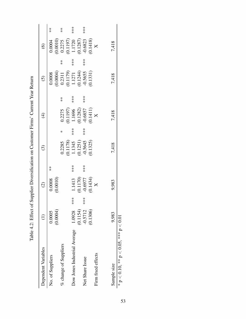
Tabl
e4.
2:E
ffec
tofS
uppl
ierD
iver
sific
atio
non
Cus
tom
erFi
rms’
Cur
rent
Yea
rRet
urn
Dep
ende
ntV
aria
bles
(1)
(2)
(3)
(4)
(5)
(6)
No.
ofSu
pplie
rs0.
0005
0.00
08**
0.00
080.
0004
**(0
.000
4)(0
.001
0)(0
.000
4)(0
.001
0)%
chan
geof
Supp
liers
0.22
85*
0.22
75**
0.23
11**
0.22
75**
(0.1
178)
(0.1
197)
(0.1
179)
(0.1
197)
Dow
Jone
sIn
dust
rial
Ave
rage
1.09
28**
*1.
1413
***
1.13
45**
*1.
1696
***
1.12
71**
*1.
1720
***
(0.1
154)
(0.1
170)
(0.1
251)
(0.1
282)
(0.1
244)
(0.1
287)
Net
Shar
eIs
sue
-0.5
712
***
-0.6
977
***
-0.5
645
***
-0.6
857
***
-0.5
655
***
-0.6
823
***
(0.1
306)
(0.1
434)
(0.1
325)
(0.1
411)
(0.1
331)
(0.1
418)
Firm
fixed
effe
cts
XX
X
Sam
ple
size
9,98
39,
983
7,41
87,
418
7,41
87,
418
*p<
0.10
,**
p<
0.05
,***
p<
0.01
53

Tabl
e4.
3:E
ffec
tofS
uppl
ierD
iver
sific
atio
non
Cus
tom
erFi
rms’
Follo
win
gY
earR
etur
n
Dep
ende
ntV
aria
bles
(1)
(2)
(3)
(4)
(5)
(6)
No.
ofSu
pplie
rs0.
0014
***
0.00
21**
0.00
15**
*0.
0031
***
(0.0
004)
(0.0
010)
(0.0
004)
(0.0
010)
%ch
ange
ofSu
pplie
rs0.
0639
0.07
840.
0686
0.07
82**
(0.1
278)
(0.1
288)
(0.1
277)
(0.1
288)
Dow
Jone
sIn
dust
rial
Ave
rage
0.21
98**
*0.
2398
***
0.21
21**
*0.
1963
***
0.19
84**
*0.
2136
***
(0.0
646)
(0.0
664)
(0.0
651)
(0.0
657)
(0.0
655)
(0.0
656)
Net
Shar
eIs
sue
-0.1
848
-0.1
595
-0.1
060
-0.1
592
-0.1
040
-0.1
827
(0.1
331)
(0.1
428)
(0.1
526)
(0.1
499)
(0.1
523)
(0.1
509)
Firm
fixed
effe
cts
XX
X
Sam
ple
size
9,98
39,
983
7,41
87,
418
7,41
87,
418
*p<
0.10
,**
p<
0.05
,***
p<
0.01
54

CHAPTER FIVE:
CONCLUSION OF DISSERTATION
This dissertation contains three independent chapters in the field of transportation, energy, and
supply chain finance economics. The first paper applies an ordered probit model to examine how
the availability of commercial truck parking potentially affects the injury severity of commercial
vehicle drivers normalized for other driving-related and environmental factors. The second paper
estimates the impacts on retail electricity price after retail electricity market restructured in the
United States. The third paper invested the impacts of downstream firms’ financial performance
with upstream supplier diversification along the supply chain.
The first paper, in Chapter 2, addresses a national safety issue related to adequate truck parking
in the United States and finds a positive relationship between truck accident severity and access to
parking facilities. With an application of the ordered probit regression method, estimation results
indicate a statistically significant relationship between commercial parking availability and truck
driver injury severity. An increase in the total number of parking spots within a thirty-minute
driving distance reduces the probability of a higher degree of personal injury and increases the
probability of a less sever injury. Several other factors impacting truck driver injury severity are
specific to the environment and driver characteristics. These include adverse surface conditions,
night driving, older driver, male drivers, and drug or alcohol involvement which all result in a
higher probability of a severe injury.
The second study, in Chapter 3, is a first application of the synthetic control method in state-
level panel data to estimate the policy impact on retail electricity price for residential, commercial,
and industrial customers from a regulatory change to introduce competition into the retail market.
We find a significant impact on all ISOs/RTOs positively or negatively, besides Oregon state. In
our analysis of intermediate factors, we find robust evidence that intervention of retail market
restructuring caused a drop in all retail prices in ISO-NE, PJM, MISO, and NYISO. This suggests
55

that the market restructuring actively provides residential end-customers freedom of choice for
utility service providers. Competition leads a lower retail price at the market equilibrium than the
regulated monopoly observed price marked in regions not utilizing restructuring. However, the
intervention of restructuring on retail market in ERCOT shows a increase of the retail price, which
is not a sign of effective for the policy.
The last paper presented in Chapter 4 studies the relationship between upstream supplier di-
versification and downstream firms’ financial performance. Regression results suggest that the
downstream firms’ return increase with an increase in the number of upstream suppliers,and fall
in major supplier’s share. Number of suppliers has a significant positive impact on find customer
firms’ returns in both the current year and following year. While the percentage change of suppliers
only positively affects current year downstream firms’ return.
56

REFERENCES
Abdel-Aty, M. (2003). Analysis of driver injury severity levels at multiple locations using ordered
probit models. Journal of safety research 34(5), 597–603.
Administration, F. M. C. S. (2006). Report to congress on the large truck crash causation study.
Alldredge, D. and A. Puckett (2016). The performance of institutional investor trades across the
supply chain. Available at SSRN 2757735.
Alldredge, D. M. and D. C. Cicero (2015). Attentive insider trading. Journal of Financial Eco-
nomics 115(1), 84–101.
Ashenfelter, O. C. and D. Card (1984). Using the longitudinal structure of earnings to estimate the
effect of training programs.
Babich, V. (2010). Independence of capacity ordering and financial subsidies to risky suppliers.
Manufacturing & Service Operations Management 12(4), 583–607.
Babich, V., A. N. Burnetas, and P. H. Ritchken (2007). Competition and diversification effects
in supply chains with supplier default risk. Manufacturing & Service Operations Manage-
ment 9(2), 123–146.
Banerjee, I., K. Jang, S. Pande, D. R. Ragland, et al. (2009). rest areas-reducing accidents involving
driver fatigue. Technical report.
Borenstein, S. and J. Bushnell (1999). An empirical analysis of the potential for market power in
california’s electricity industry. The Journal of Industrial Economics 47(3), 285–323.
Borenstein, S. and J. Bushnell (2015). The us electricity industry after 20 years of restructuring.
Annu. Rev. Econ. 7(1), 437–463.
57

Borenstein, S., J. B. Bushnell, and F. A. Wolak (2002). Measuring market inefficiencies in cali-
fornia’s restructured wholesale electricity market. American Economic Review 92(5), 1376–
1405.
Bunn, T. L., S. Slavova, and P. J. Rock (2017). Association between commercial vehicle driver at-
fault crashes involving sleepiness/fatigue and proximity to rest areas and truck stops. Accident
Analysis & Prevention.
Bushnell, J. B., S. P. Holland, J. E. Hughes, and C. R. Knittel (2017). Strategic policy choice in
state-level regulation: The epa’s clean power plan. American Economic Journal: Economic
Policy 9(2), 57–90.
Cohen, L., A. Frazzini, and C. Malloy (2008). The small world of investing: Board connections
and mutual fund returns. Journal of Political Economy 116(5), 951–979.
Cohen, M. A. and N. Agrawal (1999). An analytical comparison of long and short term contracts.
IIE transactions 31(8), 783–796.
Corsten, D. and J. Felde (2005). Exploring the performance effects of key-supplier collaboration:
an empirical investigation into swiss buyer-supplier relationships. International Journal of
Physical Distribution & Logistics Management 35(6), 445–461.
Dada, M., N. C. Petruzzi, and L. B. Schwarz (2007). A newsvendor’s procurement problem when
suppliers are unreliable. Manufacturing & Service Operations Management 9(1), 9–32.
Ellram, L. M. (1995). Partnering pitfalls and success factors. International Journal of Purchasing
and Materials Management 31(1), 35–44.
Fee, C. E. and S. Thomas (2004). Sources of gains in horizontal mergers: evidence from customer,
supplier, and rival firms. Journal of Financial Economics 74(3), 423–460.
Fu, Q., C.-Y. Lee, and C.-P. Teo (2010). Procurement management using option contracts: random
spot price and the portfolio effect. IIE transactions 42(11), 793–811.
58

Garder, P. (2006). Segment characteristics and severity of head-on crashes on two-lane rural high-
ways in maine. Accident Analysis & Prevention 38(4), 652–661.
Graf, C. and D. Wozabal (2013). Measuring competitiveness of the epex spot market for electricity.
Energy Policy 62, 948–958.
Guan, Y., M. F. Wong, and Y. Zhang (2015). Analyst following along the supply chain. Review of
Accounting Studies 20(1), 210–241.
Hadsell, L. and H. A. Shawky (2007). One-day forward premiums and the impact of virtual bidding
on the new york wholesale electricity market using hourly data. Journal of Futures Markets:
Futures, Options, and Other Derivative Products 27(11), 1107–1125.
Hanowski, R. J., J. Hickman, M. C. Fumero, R. L. Olson, and T. A. Dingus (2007). The sleep of
commercial vehicle drivers under the 2003 hours-of-service regulations. Accident Analysis
& Prevention 39(6), 1140–1145.
Hertzel, M. G., Z. Li, M. S. Officer, and K. J. Rodgers (2008). Inter-firm linkages and the wealth
effects of financial distress along the supply chain. Journal of Financial Economics 87(2),
374–387.
Irvine, P. J., S. S. Park, and C. Yıldızhan (2015). Customer-base concentration, profitability, and
the relationship life cycle. The Accounting Review 91(3), 883–906.
Johnston, D. A., D. M. McCutcheon, F. I. Stuart, and H. Kerwood (2004). Effects of supplier
trust on performance of cooperative supplier relationships. Journal of operations Manage-
ment 22(1), 23–38.
Joskow, P. and E. Kahn (2001). A quantitative analysis of pricing behavior in california’s whole-
sale electricity market during summer 2000. In 2001 Power Engineering Society Summer
Meeting. Conference Proceedings (Cat. No. 01CH37262), Volume 1, pp. 392–394. IEEE.
59

Joskow, P. L. (2006). Competitive electricity markets and investment in new generating capacity.
Massachusetts Institute of Technology (MIT)-Department of Economics.
Khattak, A., P. Kantor, and F. Council (1998). Role of adverse weather in key crash types on
limited-access: roadways implications for advanced weather systems. Transportation Re-
search Record: Journal of the Transportation Research Board (1621), 10–19.
Kleindorfer, P. R. and D. J. Wu (2003). Integrating long-and short-term contracting via business-to-
business exchanges for capital-intensive industries. Management Science 49(11), 1597–1615.
Kockelman, K. M. and Y.-J. Kweon (2002). Driver injury severity: an application of ordered probit
models. Accident Analysis & Prevention 34(3), 313–321.
Kwoka, J. (2008). Restructuring the us electric power sector: A review of recent studies. Review
of Industrial Organization 32(3-4), 165–196.
Lee, C. and M. Abdel-Aty (2008). Presence of passengers: does it increase or reduce driver’s crash
potential? Accident Analysis & Prevention 40(5), 1703–1712.
Li, C. and L. G. Debo (2009). Strategic dynamic sourcing from competing suppliers with transfer-
able capacity investment. Naval Research Logistics (NRL) 56(6), 540–562.
Lian, Y. (2017). Financial distress and customer-supplier relationships. Journal of Corporate
Finance 43, 397–406.
Longstaff, F. A. and A. W. Wang (2004). Electricity forward prices: a high-frequency empirical
analysis. The journal of finance 59(4), 1877–1900.
Maldonado, C., D. Mitchell, S. Taylor, and H. Driver (2002). Sleep, work schedules and accident
risk in south african long-haul truck drivers: research in action. South African Journal of
Science 98(7-8), 319–324.
Martin, J. H. and B. Grbac (2003). Using supply chain management to leverage a firm’s market
orientation. Industrial marketing management 32(1), 25–38.
60

Martınez-de Albeniz, V. and D. Simchi-Levi (2006). Mean-variance trade-offs in supply contracts.
Naval Research Logistics (NRL) 53(7), 603–616.
McKelvey, R. D. and W. Zavoina (1975). A statistical model for the analysis of ordinal level
dependent variables. Journal of mathematical sociology 4(1), 103–120.
Menzly, L. and O. Ozbas (2010). Market segmentation and cross-predictability of returns. The
Journal of Finance 65(4), 1555–1580.
Morris, P. and K. O’Brien (2007). Safety rest area spacing and vehicle crash rates: is there a
minnesota connection? National Safety Rest Area Conference.
Morris, T., T. Henderson, V. Morellas, and N. Papanikolopoulos (2018). A real-time truck avail-
ability system for the state of wisconsin.
Pandit, S., C. E. Wasley, and T. Zach (2011). The effect of research and development (r&d) inputs
and outputs on the relation between the uncertainty of future operating performance and r&d
expenditures. Journal of Accounting, Auditing & Finance 26(1), 121–144.
Pirrong, C. and M. Jermakyan (1999). Valuing power and weather derivatives on a mesh using
finite difference methods. Energy Modelling and the Management of Uncertainty, 59–69.
Radun, I. and H. Summala (2004). Sleep-related fatal vehicle accidents: characteristics of deci-
sions made by multidisciplinary investigation teams. Sleep 27(2), 224–227.
Saravia, C. (2003). Speculative trading and market performance: the effect of arbitrageurs on
efficiency and market power in the new york electricity market.
Su, X. (2015). Have customers benefited from electricity retail competition? Journal of regulatory
economics 47(2), 146–182.
Swinney, R. and S. Netessine (2009). Long-term contracts under the threat of supplier default.
Manufacturing & Service Operations Management 11(1), 109–127.
61
Taylor, W., N. Sung, and A. Jawad (1999). A study of highway rest areas and fatigue related truck
crashes. In 78th Transportation Research Board Annual Meeting, Washington, DC.
Tefft, B. C. (2010). Asleep at the wheel: The prevalence and impact of drowsy driving.
Tomlin, B. and Y. Wang (2005). On the value of mix flexibility and dual sourcing in unreliable
newsvendor networks. Manufacturing & Service Operations Management 7(1), 37–57.
Van Doren, P. and J. Taylor (2004). Rethinking electricity restructuring. Cato Institute.
Wolak, F. A., R. Nordhaus, and C. Shapiro (2000). An analysis of the june 2000 price spikes in the
california iso’s energy and ancillary services markets. California ISO Market Surveillance
Committee, Sep 6.
Wu, Z. and T. Y. Choi (2005). Supplier–supplier relationships in the buyer–supplier triad: Building
theories from eight case studies. Journal of Operations management 24(1), 27–52.
Xie, Y., Y. Zhang, and F. Liang (2009). Crash injury severity analysis using bayesian ordered
probit models. Journal of Transportation Engineering 135(1), 18–25.
Yamamoto, T. and V. N. Shankar (2004). Bivariate ordered-response probit model of driver’s and
passenger’s injury severities in collisions with fixed objects. Accident Analysis & Preven-
tion 36(5), 869–876.
Yang, Z., G. Aydın, V. Babich, and D. R. Beil (2012). Using a dual-sourcing option in the pres-
ence of asymmetric information about supplier reliability: Competition vs. diversification.
Manufacturing & Service Operations Management 14(2), 202–217.
Ye, F. and D. Lord (2014). Comparing three commonly used crash severity models on sample size
requirements: multinomial logit, ordered probit and mixed logit models. Analytic methods in
accident research 1, 72–85.
Zhu, X. and S. Srinivasan (2011). A comprehensive analysis of factors influencing the injury
severity of large-truck crashes. Accident Analysis & Prevention 43(1), 49–57.
62