three essays on development economics and...
TRANSCRIPT

Three Essays on Development Economics and
Environmental Economics
by
Yu Benjamin Fu
M.A. (Economics), Carleton University, 2005 B.A., Wuhan University, 1997
Dissertation Submitted in Partial Fulfillment
of the Requirements for the Degree of
Doctor of Philosophy
in the
Department of Economics
Faculty of Arts and Social Sciences
Yu Fu 2012
SIMON FRASER UNIVERSITY
Fall 2012
All rights reserved. However, in accordance with the Copyright Act of Canada, this work may
be reproduced, without authorization, under the conditions for “Fair Dealing.” Therefore, limited reproduction of this work for the
purposes of private study, research, criticism, review and news reporting is likely to be in accordance with the law, particularly if cited appropriately.

ii
Approval
Name: Yu Fu
Degree: Doctor of Philosophy (Economics)
Title of Thesis: Three Essays on Development Economics and Environmental Economics
Examining Committee:
Chair: Simon Woodcock Associate Professor, Department of Economics
Kenneth Kasa Senior Supervisor Professor, Department of Economics
Terry Heaps Supervisor Associate Professor, Department of Economics
Alexander Karaivanov Supervisor Associate Professor, Department of Economics
George Zhang Supervisor Professor, Faculty of Business Administration
Payman Jula Internal Examiner Associate Professor, Faculty of Business Administration
Wendy Wu External Examiner Associate Professor, Department of Economics Wilfrid Laurier University
Date Defended/Approved: October 22nd, 2012

iii
Partial Copyright Licence

iv
Abstract
This thesis consists of three independent essays on the fields of development
economics and environmental economics. The first two papers use the same theoretical
model to explain different issues in developing countries. The third paper studies the
effects of population growth on the Environmental Kuznets Curve provided it exists.
China's internal migration plays an important role in explaining its recent economic
success. The first paper constructs a model of labor migration, focusing on the role of
selection effects in determining labor market outcomes, and then calibrates it to quantify
the effects of China's labor market reforms on its outputs and inequality. I show that the
removal of internal migration restrictions benefits the economy as a whole, while
exacerbating inequality within both rural and urban areas.
The second paper suggests that minimum wage policy may be beneficial for a
transitional economy in which labor is migrating from rural areas to urban areas when
positive moving costs occur. With a moving cost wedge a modestly binding minimum
wage can cause relatively low productivity urban workers to be replaced by higher
productivity rural migrants, and therefore increase aggregate output. To achieve the
second best outcome, government shall fully compensate the moving costs for the
marginal migrant workers who move from the rural industrial sector to the urban
subsistence sector and a binding minimum wage shall be imposed on the urban workers
but not the migrant workers in the urban industrial sector.
The Environmental Kuznets Curve (EKC) hypothesis postulates an inverted U-shaped
relationship between economic growth and many local environmental health indicators.
By using an overlapping generations (OLG) model, I focus on technological effects,
where the properties of the existing pollution abatement technologies could generate the
inverted U-shaped EKC and other forms of growth-pollution paths for the less advanced
economies. Moreover, I examine the effects of population growth on the shape of the
EKC, provided that it exists. Simulations indicate positive population growth raises the
height of the EKC at every level of output per worker; thus, putting an extra burden on
environment quality. Empirical evidence from China partially supports the results.

v
Keywords: Migration; selection; minimum wage; Environmental Kuznets Curve; Technological effects; China

vi
Dedication
I dedicate this dissertation to my family, especially…
To grandma and grandpa, for opening my eyes to the world;
To Dad and Mom, for your inspiration and support;
To Danni and Zeke, for all the time we have spent.

vii
Acknowledgements
My deepest gratitude is to my senior supervisor, Dr. Kenneth Kasa. I have not only
learned economic theories and methodologies from him but also the attitudes towards
doing research which will be the most valuable assets for my future career. I am grateful
to him for his high research standard and enforcing strict validations for each research
result, and thus teaching me how to do research.
I am indebted to Dr. Terry heaps for all his support. He gave me many valuable advices
and kept me updated with the latest research papers. I am also thankful to him for
carefully reading my paper and checking all mathematical proofs. His patience and
guidance are priceless.
I am grateful to Dr. Alex Karaivanov. He was always there when I needed advice. I had
been benefited from his clear instructions. His insightful comments and constructive
criticisms often opened new windows to me which not only sorted out the details of my
work but also pointed out the potential extensions. His knowledge, attitude and work
ethic make him a typical example for the young scholars.
Dr. George Zhang is more than a supervisor for me. His support is all-round. He taught
me methodologies which are very important for my research. Moreover, he helped me
overcome many difficult situations, both academically and personally. It has been my
great fortune to meet him at Simon Fraser University. I owe sincere and earnest thanks
to him and Mrs. Sue Su.
I am also grateful to all the faculties and colleagues who had given me suggestions or
had discussions, especially Dr. David Andolfatto, Dr. Yi Xue and Dr. Sophie Wang.
Great deals appreciated go to the contribution of the Department’s supporting staff,
especially Kathleen Vieira-Ribeiro, Gwen Wild, and Tim Coram who are patient in
helping me throughout this degree.
I would like to acknowledge NSERC grant support (RGPIN197319).

viii
Table of Contents
Approval .............................................................................................................................ii Partial Copyright Licence .................................................................................................. iii Abstract .............................................................................................................................iv Dedication .........................................................................................................................vi Acknowledgements .......................................................................................................... vii Table of Contents ............................................................................................................ viii List of Tables ..................................................................................................................... x List of Figures....................................................................................................................xi
Chapter 1. China's Internal Migration: A theoretical and Numerical Analysis .................................................................................................... 1
1.1 Introduction ................................................................................................................. 1 1.2 Background ................................................................................................................. 4 1.3 Model setup................................................................................................................. 9
1.3.1 Model assumptions ......................................................................................... 9 1.3.2 Restricted labor mobility ................................................................................ 11 1.3.3 Unrestricted labor mobility ............................................................................. 14
1.4 Quantitative analysis ................................................................................................. 21 1.4.1 Parameters and functions ............................................................................. 22 1.4.2 Restricted labor mobility ............................................................................... 25 1.4.3 Unrestricted labor mobility ............................................................................ 26 1.4.4 Welfare change ............................................................................................. 32
1.5 Policy implication ....................................................................................................... 33 1.6 Conclusion ................................................................................................................ 35 1.7 References ................................................................................................................ 38 1.8 Appendices .............................................................................................................. 40
Appendix 1.A Relative price forming ...................................................................... 40 Appendix 1.B Mathmatical equilibrium in figure 1.6 ............................................. 41
Appendix 1.C Mathmatical equilibrium in figure 1.6 ............................................. 42
Chapter 2. The Economic Effects of Minimum Wage Policy ................................. 44 2.1 Introduction ............................................................................................................... 44 2.2 Model setup............................................................................................................... 47
2.2.1 Model assumptions ....................................................................................... 47 2.2.2 The best outcomes ........................................................................................ 48 2.2.3 The market equilibrium outcome .................................................................. 49
2.3 Minimum wage .......................................................................................................... 57 2.4 Quantitative analysis ................................................................................................. 60
2.4.1 Calibration ..................................................................................................... 60 2.4.2 The second best outcome ............................................................................. 63 2.4.3 The market equilibrium outcome ................................................................... 65
2.4.3.1 The equations system ....................................................................... 65 2.4.3.2 Simulations ........................................................................................ 66 2.4.3.3 Welfare change ................................................................................. 70
2.5 Policy implication ....................................................................................................... 72

ix
2.6 Conclusion ................................................................................................................ 74 2.7 References ................................................................................................................ 77 2.8 Appendices .............................................................................................................. 80
Appendix 2.A Relative price forming ...................................................................... 80 Appendix 2.B Mathmatical equilibrium in figure 2.3 ............................................. 80
Appendix 2.C Mathmatical equilibrium in figure 2.3 ............................................. 82
Chapter 3. Population Growth and the Environmental Kuznets Curve ................ 84 3.1 Introduction ............................................................................................................... 84 3.2 Model ....................................................................................................................... 87
3.2.1 Assumptions .................................................................................................. 87 3.2.2 Model analysis .............................................................................................. 89
3.3 Positive population growth ........................................................................................ 97 3.4 Simulations.............................................................................................................. 101 3.5 Empirical evidence .................................................................................................. 106 3.6 Concluding remarks ................................................................................................ 111 3.7 References .............................................................................................................. 112 3.8 Appendices ............................................................................................................ 115
Appendix 3.A Proof of proposition 3.1 .................................................................. 115 Appendix 3.B Proof of proposition 3.3 .................................................................. 116 Appendix 3.C Proof of proposition 3.5 ................................................................. 117 Appendix 3.D The basic statistics of the data ...................................................... 119

x
List of Tables
Table 1.1. Percentage of residents with corresponding highest degree ....................... 5
Table 1.2. Distribution of labor force and migration workers ......................................... 8
Table 1.3. Blue vs. White collar industries: percentage of migrant workers with corresponding highest degree obtained .................................................. 9
Table 1.4. Facts and parameters ................................................................................ 22
Table 1.5. Equilibrium outcomes: restricted labor with career options ........................ 25
Table 1.6. Equilibrium outcomes: unrestricted labor with career options .................... 27
Table 1.7. The effects on output ................................................................................. 28
Table 1.8. The effects of removing labor constraint on inequalities ............................ 29
Table 1.9. Comparison between the model and data.................................................. 31
Table 1.10 Welfare change after the labor mobility constraint is removed ................... 33
Table 2.1. Equilibrium outcomes when minimum wage is enforced ............................ 68
Table 2.2. The effects of minimum wage on output values ......................................... 69
Table 2.3. Equilibrium outcomes: restricted labor with career options ........................ 70
Table 2.4. Welfare change after w = 0.4814 is enforced ............................................ 71
Table 2.5. Welfare change after w = 0.4900 is enforced ............................................. 72
Table 3.1. The output of the fixed-effect model for three pollutants .......................... 108
Table 3.D1 The yearly averages of the panel data ..................................................... 119

xi
List of Figures
Figure 1.1. The evolution of China’s Gini coefficients .................................................... 7
Figure 1.2. Distribution of labor force and migration workers ......................................... 8
Figure 1.3. Occupation allocations without labor mobility ............................................. 14
Figure 1.4. Equilibrium human capital thresholds ........................................................ 17
Figure 1.5. Heading to the US sector ........................................................................... 19
Figure 1.6. Career distribution in the rural region ......................................................... 20
Figure 1.7. Career distributions before and after the labor mobility constraint is removed ..................................................................................................... 32
Figure 2.1. Equilibrium human capital thresholds ........................................................ 52
Figure 2.2. Heading to the US sector ........................................................................... 54
Figure 2.3. Career distribution in rural areas ................................................................ 56
Figure 2.4. The effects of minimum wage on urban workers ........................................ 58
Figure 2.5. The effects of minimum wage on utility and output .................................... 67
Figure 2.6. Welfare change after w = 0.4814 is enforced ............................................ 72
Figure 2.7. Welfare change after w = 0.4900 is enforced ............................................. 73
Figure 3.1. The time path of z .................................................................................... 103
Figure 3.2. The time path of output ............................................................................ 103
Figure 3.3. The time path of pollution ......................................................................... 104
Figure 3.4. The time path of environmenal quality ..................................................... 104
Figure 3.5. The EKC ................................................................................................... 104
Figure 3.6. The E-output trace ................................................................................... 104
Figure 3.7. The time paths of z ................................................................................... 105
Figure 3.8. The time paths of pollution ....................................................................... 105
Figure 3.9. The time paths of environmental quality................................................... 105

xii
Figure 3.10. The EKCs ................................................................................................. 105
Figure 3.11. The EKCs of SO2 ..................................................................................... 110
Figure 3.12. The EKCs of waste water ......................................................................... 110
Figure 3.13. The EKCs of waste gas ............................................................................ 110

1
Chapter 1. China's Internal Migration: A theoretical and Numerical Analysis
1.1 Introduction
China's economy has been the focus of the world in recent decades. Its economy
has maintained a very high growth rate, even during the recent worldwide financial crisis.
Among the efforts to explain China's achievements, many economists focus on the role
of China's internal migration (Zhang and Song, 2004; Du et al, 2005; Au and Henderson,
2006). Barriers to labor mobility throughout the country have been continuously lowered
since the beginning of China's economic reform in the early 1980s. Because of the
substantial income differential between rural and urban areas, we have observed a flow
of migrant workers from poor rural areas to rich urban ones occurring coincidentally with
China's economic growth.1
Until recently, most studies of China's internal migration and growth have been
predominantly empirical. Du et al (2005) use data from the China Poverty Monitoring
Survey (CPMS) and the China Rural Poverty Survey (CRPS) and find an inverted-U-
1 China officially relaxed its labor mobility constraints in 1985. By the end of 2008, the number of
migrant workers reached 140.41 million while China's real GDP of 2008 was 8.6 times as that of 1985. (China Statistical Yearbook 1986, 2009)

2
shaped relationship between household endowments and the likelihood of migration.2
Whalley and Zhang (2007) calibrate a model with homogeneous labour in which
inequality of wages is only supported by domestic migration restrictions. Although these
authors offer explanations of their findings, they focus on empirical issues. In this paper,
I instead build and calibrate a structural model to examine the effects of China's labor
market reforms. The model generates two key predictions that are consistent with
observed outcomes in China: (1) China's great success on poverty reduction has been
very uneven; and (2) domestic migration enhanced China's inequality in both rural and
urban areas.3
My analysis takes place in two main steps: the first is to develop a theoretical
model of labor migration with heterogeneous agents, in the tradition of the well-known
Roy (1951) model, which focuses on the role of selection effects in determining labor
market outcomes. In doing so, my model differs in some important respects from
standard analyses of migration and inequality, which are typically based on of the Harris-
Todaro (1970) model. In my model, migrants confront no uncertainty concerning their
urban prospects. By construction then, all movers gain. Inequality is not caused by the
varying fortunes of urban job-seekers, but rather from the interaction of selection and
general equilibrium wage effects.4
The second key step of my analysis is to follow the tradition of the applied
general equilibrium literature in order to quantify the effects of China's labor market
2 Du et al (2005) defines endowments as a set of variables consisting of the highest year of
education, cultivated land per capita, household size, the share of household members that is laborers, the share of household members that is children, and village dummy variables that capture geographic and other community endowments that affect migration. Fitted income is used as an index of exogenous household endowments in which each endowment is weighted by its relative importance to income generation.
3 Ravallion and Chen (2007) contains an excellent review of China's economy.
4 Note, in traditional applications of the Roy model to labor markets, general equilibrium wage
effects are abstracted from. See Borjas (1987) for an application of the Roy model to U.S. immigration.

3
reforms.5 I begin by calibrating my model's parameters to match labor market outcomes
in China in 1986. The assumption is that this represents the starting date of China's
relaxed labor mobility restrictions. I then simulate the effects of enhanced labor mobility
by reducing the costs of migration, while holding constant the remaining parameters. I
abstract from transition dynamics by assuming that a new steady state was reached by
the year 2006. I find that if migration costs are inversely related to skill level, then the
combination of selection and general equilibrium wage effects can explain,
quantitatively, why we have observed a simultaneous increase in both urban and rural
inequality. Loosely speaking, once internal migration restrictions are removed, the most
skilled rural workers migrate to urban areas. This exacerbates inequality in rural areas
because it makes skilled workers scarce in rural areas, which raises the relative wages
of the relatively wealthiest rural residents. At the same time, the influx of rural migrants
has a disproportionately negative supply-side effect on the wages of the lower end of the
urban skill distribution, driving down the relative wages of the poorest urban residents.
Although my model explains the within-area inequality change, it cannot explain
observed rising urban-rural inequality. This primarily reflects exogenous disparities in
government-directed fixed investment. Because many rural workers move from a low
productivity agricultural sector to comparatively high productivity industrial sectors, the
removal of migration barriers benefits the whole economy.
The rest of this paper is organized as follows. Section 1.2 briefly reviews
necessary institutional background knowledge about China. Section 1.3 contains the
model setup and analysis. Section 1.4 provides calibrations and simulations of my
model. Section 1.5 discusses some potential policy implications. Section 1.6 concludes,
and suggests some potential extensions.
5 Shoven and Whalley (1992) contains an overview of this methodology.

4
1.2 Background
This section introduces necessary institutional background knowledge about
China. The facts mentioned below are either consistent with my model assumptions or
the model results.
1. Model assumption: urban areas and rural areas have received very uneven
capital investment from the central government.
Facts: China's central government adopted a dual-sector development
strategy soon after the People's Republic of China was founded in 1949 and land
reforms were completed in 1952. Rural areas were only allowed to engage in agriculture,
while capital intensive heavy industries were mostly developed in cities. Consequently,
China's urban areas and rural areas have received very uneven capital investment from
the central government. Meanwhile, most of China's population lived in rural areas
especially before economic reform started. By the time economic reform began in 1978,
the agricultural sector accounted for less than 12% of total investment but employed
about 80% of the total labor force. During the period 1952--1990, the value of industrial
sector output increased by 65 times, whereas agricultural sector output increased by
only 3 times.6
2: Model assumption: urban areas and rural areas have different distributions
of human capital.
Facts: Because human capital differences are a key component in my model,
and education has significant effects on human capital, we must consider differences
between urban and rural areas in the level of education. Table 1.1 indicates this
difference in 2000.7 Because of existing quality differences between rural and urban
6 Numbers are quoted from Yao (1994).
7 Data source: Fifth National Census conducted by Statistics China.

5
education, these numbers likely understate the true difference between rural and urban
education.
Table 1.1. Percentage of residents with corresponding highest degree
Elementary school or lower Middle school Post-secondary degree
Urban 16.83 69.20 13.97
Rural 47.62 51.67 0.71
3: Model assumption: physical labor mobility constraints first existed, and then
were removed and replaced by institutional and economic barriers.
Facts: To ensure the implementation of its urban-biased investment plan, China's
government imposed many restrictions on rural residents. The most famous is the
Hukou (residency registration) system, which gives every Chinese her own internal
"citizenship". People were forbidden to live and work in an area without government
permission if they didn't own local Hukou. Hukou entitled its holders to local access to
job opportunities, education and medical resources, and other social benefits which
differed significantly between urban and rural areas. China's government began using
this system in 1958 to control the movement of people, and it was strictly enforced until
the start of the economic reform through regulations which authorized police to detain
people and repatriate them to their permanent residency location. Economic reforms
created incentives for migration from rural to urban areas. Beginning in the late 1980s,
the increased openness of China to the rest of the world triggered another wave of
expansion in the industrial sector. The huge demand for labor which resulted made legal
restrictions on labor mobility no longer sustainable. The Hukou system officially
remained, but its role of physical restrictions was removed. Legal constraints were
replaced by institutional and economic barriers. For example, in some cities many job
positions are only provided to job-seekers with local Hukous; in other cases firms must

6
pay the government for permission to hire a worker without local Hukou.8 The
government officially relaxed this restriction in 1985, allowing people to live in areas in
which they did not own local Hukou. However, some conditions still applied. For
example, they had to apply for a temporary residency permit from local police. This
system underwent further relaxation during the mid-1990s as China pursued entry to
GATT (the predecessor of WTO), and promised to further liberalize the movement of
labor to speed up its economic reform. In 2003, the laws on custody and repatriation
were repealed.9 However, even with legal mobility restrictions removed, most welfare
benefits are still exclusively provided to residents with local Hokous.
4: Model result: inequality has increased within both rural and urban areas
over time.
Facts: Less development combined with a huge population put rural residents
in a very disadvantaged position. For example, in 1950, the ratio between urban and
rural nominal income per capita was about 2:1. By the time economic reform started in
1978, this ratio had increased to 2.56. By 2007 it had further increased to 3.33.10 Many
economists argue that this ratio is actually underestimated because of allowances and
social welfare provided exclusively to urban citizens.11
The Gini coefficients for the whole of China, and for urban and rural areas, were
0.2927, 0.2504, and 0.1712 in 1981, 0.3587, 0.3221, and 0.2319 in 1990, and 0.4419,
0.3637, and 0.3263 in 2004. These facts point to not only a widening gap between urban
8 "In Beijing...at least 35 types of jobs would be closed to migrants. Urban employers are also
required to pay a per capita fee for each migrant they hire..." See Wang and Zuo (1999). 9 Au and Henderson (2006) and Lu (2002) have more detailed discriptions about China's Hukou
system. 10
People's Daily online resource: Special Focus: 3:33 to 1! The gap between urban and rural areas is larger than ever.
11 Naughton (2007): from the mid-1960s until well into the 1990s, urban residents received the
following benefits: job security; guaranteed low-price access to food grains, as well as other scarce commodities; health care; a pension and other benefits, including health care, upon retirement; primary and middle school education for their children; low-cost housing, supplied by the work unit.

7
and rural areas but also to inequality increases within both areas. My model focuses on
the growing inequality within the rural and urban sectors. Figure 1.1 illustrates these
developments. 12
Figure 1.1. The evolution of China’s Gini coefficients
5. Model result: migration flows increase with lower labor mobility constraints.
Facts: after legal mobility constraints were abandoned, more and more rural
workers left home to work in urban areas.13 In 1999, 81% of total migrants and 89% of
interprovincial migrants came from inland areas, and most inland migration (72%) was
interprovincial.14 In 1996, the total number of migrant workers from rural areas was 72.22
12 Numbers are quoted from Table 1 in Cheng (2007).
13 We may observe city-to-country migration flow as there are many cities in traditional rural areas
and many countries in traditional urban areas in China. 14
See Zhang and Song (2003).
0.1
0.15
0.2
0.25
0.3
0.35
0.4
0.45
0.5
19
81
19
82
19
83
19
84
19
85
19
86
19
87
19
88
19
89
19
90
19
92
19
93
19
94
19
95
19
96
19
97
19
98
19
99
20
00
20
01
20
02
20
03
20
04
National Gini Rural Gini

8
million. By 2006, this number had increased to 131.81 million.15 But the demography is
changing: in 1996 we observed more migrant workers from eastern China than in central
and western China, while 10 years later most migrant workers came from central and
western China. Table 1.2 summarizes this information.16
Table 1.2. Distribution of rural labor force and migration workers
E.China(96) E.China(06) C.China(96) C.China(06) W.China(96) W.China(06)
Rural labor force
224.26 198.28 194.34 145.82 142.25 151.42
Migrant workers
34.04 38.46 23.43 49.18 14.74 40.35
% of migrant workers
15.18 19.40 12.06 33.72 10.36 26.65
6. Model result: rural migrant workers with high human capital move to the
urban industrial sector, while those with low human capital move to the urban
subsistence sector.
Facts: Another noticeable fact is the disparity in education levels between
workers employed in different urban sectors. Zhang and Lei (2008) conducted a survey
of 600 migrant workers in white-collar industries in Shanghai. They found that 82.8% had
post-secondary degrees. Pan and Sun (2008) looked at a sample of 1200 migrant parent
workers in blue-collar industries in Zhejiang province and found that most blue-collar
15
The First and Second National Agricultural Census, Statistics China (2001, 2008). The Communique of key data from Second National Agricultural Census, Statistics China (2008). Rural labor force refers to rural residents older than 16 who are capable of working; migrant workers refer to those who worked outside their home town for at least one month in 2005.
16 Numbers are in millions except percentage terms. All numbers are quoted from The First and
Second National Agriculture Census conducted by Statistics China.
9
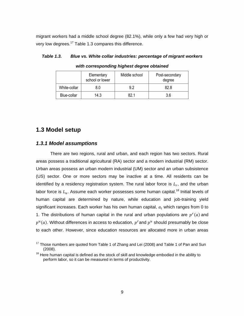
migrant workers had a middle school degree (82.1%), while only a few had very high or
very low degrees.17 Table 1.3 compares this difference.
Table 1.3. Blue vs. White collar industries: percentage of migrant workers
with corresponding highest degree obtained
Elementary school or lower
Middle school Post-secondary degree
White-collar 8.0 9.2 82.8
Blue-collar 14.3 82.1 3.6
1.3 Model setup
1.3.1 Model assumptions
There are two regions, rural and urban, and each region has two sectors. Rural
areas possess a traditional agricultural (RA) sector and a modern industrial (RM) sector.
Urban areas possess an urban modern industrial (UM) sector and an urban subsistence
(US) sector. One or more sectors may be inactive at a time. All residents can be
identified by a residency registration system. The rural labor force is , and the urban
labor force is . Assume each worker possesses some human capital.18 Initial levels of
human capital are determined by nature, while education and job-training yield
significant increases. Each worker has his own human capital, which ranges from 0 to
1. The distributions of human capital in the rural and urban populations are ( ) and
( ). Without differences in access to education, and should presumably be close
to each other. However, since education resources are allocated more in urban areas
17
Those numbers are quoted from Table 1 of Zhang and Lei (2008) and Table 1 of Pan and Sun (2008).
18 Here human capital is defined as the stock of skill and knowledge embodied in the ability to
perform labor, so it can be measured in terms of productivity.

10
and there are uneven opportunities to access to post-secondary education, is
assumed to exhibit first-order stochastic dominance over , as shown in Figure 1.2.
Figure 1.2. Human capital distributions
In the RA sector, labor is considered homogenous, and the production function
is:
( ) (1.1)
where is total physical labor input. Because land is limited, . Farmers are
paid at their marginal product of labor and the government takes all the remaining as
landowner.
In the industrial sectors, I assume agents produce according to a constant-
return-to-scales production functions and are paid their marginal product. Each worker's
production function in UM and RM are:
( ) (1.2)
( ) (1.3)
where is the human capital possessed by worker , and is the physical labor input of
each worker, which is normalized to 1. and differ in terms of productivity and
resource-intensity. I assume that UM sector has higher productivity and its technology is
more capital intensive. Note that I assume total capital investment in both industrial
sectors is equally distributed among the workers, and . The
marginal product of labor, , is increasing with and as capital and labor are
11
partially complements. Government allocation of investment between sectors is
assumed to be exogenous and . Manufactured goods are homogeneous.
The relative price between agricultural goods and industrial goods, , clears
the market. Manufactured goods are defined as the numeraire. The price function is:
(
) (1.4)
with ( ) and where is the output of RA sector and is the output of
manufacturing sector.19 Since the manufacturing sector is only set up in the urban area,
equals the output of UM.
This starting point is designed to mimic a planned economy. There is no
physical investment in rural areas, and labor mobility is strictly prohibited. Modern
industry is confined to urban areas, and rural areas can only engage in traditional
agriculture (i.e., rural areas only have an RA sector and urban areas only have a UM
sector).
1.3.2 Restricted labor mobility
The timing of this stage corresponds to the start of economic reform, during
which labor mobility was still restricted, but workers could choose freely between local
job options. In rural areas, the RM sector is developed with some exogenous physical
investment, which is nonetheless much less than in urban areas. Farmers are allowed to
leave the RA sector, but can only work locally. Because RM has lower productivity and
less physical capital per capita than UM, its MPN is smaller than in UM at any given level
of human capital.
19
One possible way to endogenize it is to assume homogeneous preference over both agricultural and industrial goods (e.g. Cobb-Douglas). Given a relative price level, the consumption ratio is constant, and should be proportional to the ratio of outputs when the market clears. Thus relative price is negatively related to the ratio of outputs. Please refer to Appendix 1.A.

12
Inequality appears after career options are allowed, because higher human-
capital workers earn no less than workers with less human capital. The equilibrium can
be derived as follows: rural workers can choose to be farmers or enter the RM sector. In
the RM sector, each worker produces and gets paid her . As is normalized
to 1, her total income is:
( ) (1.5)
( ) is an increasing function of both and which implies workers with
more
human capital are more likely to work in the RM sector. Career decisions of rural
workers are analyzed by comparing incomes from each sector. In equilibrium, the worker
who is indifferent between working in RA or RM must possess human capital , which
is determined by:
( ) (
) (1.6)
where ∫ ( )
is employment in the RA sector, ∫ ( )
is
employment in the RM sector and is the exogenous capital investment in rural areas.
is the relative price given by:
(
) (1.7)
where the outputs of RA and RM sectors are:
( ∫
) (1.8)
∫ ( )
(1.9)
and is defined in equation (1.13). Therefore, rural workers with more human capital
than choose to work in the local industrial sector.
In urban areas, the US sector emerges at this stage to employ workers who are
not productive enough to enter the UM sector. In the US sector, workers provide

13
services for people in the UM sector. Such work ranges from domestic employment to
low-skill positions in industry. In the UM sector the worker with the least human capital
must be indifferent between entering UM or US. Assume her human capital is . Her
wage if she works in UM is:
( ) (1.10)
where is the exogenous physical investment per capita, and
∫ ( )
. is an increasing function of .
In the US sector, I assume all workers work independently with a linear
production function. Total output is:
(1.11)
where is employment in US, which is a function of . In this sector, everyone gets
paid at . Because is affected by total income of the people in UM (demand) and
the labor supply in US (supply), the US wage function is:
( ) (1.12)
with ( and ( ) .
Output of the UM sector is:
∫ ( )
(1.13)
It is a function of , as is . More specifically is a decreasing function of
, because skill doesn't matter in US. Therefore a unique value of can be inferred
from the equilibrium condition:
( ) ( ) (1.14)
A real root can be ensured provided that ( ) ( ) and
( ) ( ).
14
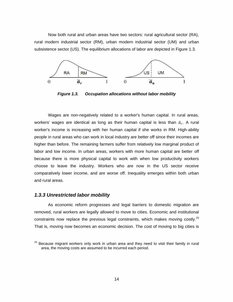
Now both rural and urban areas have two sectors: rural agricultural sector (RA),
rural modern industrial sector (RM), urban modern industrial sector (UM) and urban
subsistence sector (US). The equilibrium allocations of labor are depicted in Figure 1.3.
Figure 1.3. Occupation allocations without labor mobility
Wages are non-negatively related to a worker's human capital. In rural areas,
workers' wages are identical as long as their human capital is less than . A rural
worker's income is increasing with her human capital if she works in RM. High-ability
people in rural areas who can work in local industry are better off since their incomes are
higher than before. The remaining farmers suffer from relatively low marginal product of
labor and low income. In urban areas, workers with more human capital are better off
because there is more physical capital to work with when low productivity workers
choose to leave the industry. Workers who are now in the US sector receive
comparatively lower income, and are worse off. Inequality emerges within both urban
and rural areas.
1.3.3 Unrestricted labor mobility
As economic reform progresses and legal barriers to domestic migration are
removed, rural workers are legally allowed to move to cities. Economic and institutional
constraints now replace the previous legal constraints, which makes moving costly.20
That is, moving now becomes an economic decision. The cost of moving to big cities is
20
Because migrant workers only work in urban area and they need to visit their family in rural area, the moving costs are assumed to be incurred each period.

15
not just pecuniary, but also includes loneliness, discrimination from urban residents,
safety issues, etc.21 Assuming high-skilled people adapt to a new environment faster, the
cost of moving is modeled as a decreasing function of . The moving cost is also
affected by the locations of rural areas, traffic conditions, and other factors. The effect of
different locations and/or traffic conditions of rural areas on the migration decision is
shown below in figure 1.5c. In this paper I assume human capital is the key determinant,
and assume the cost of moving is ( ) with ( ) .22
When a rural worker considers moving, she compares the benefits of moving to
the cost. By assuming that a higher wage is the benefit she would earn if working in an
urban area, her net benefit function is:
( ) ( ) ( ) (1.15)
I assume that ( ) ( ) ( ) , i.e.
( ( ∫
)) ( )
( ( ∫
)) (1.16)
to make sure that at least the highest ability rural worker obtains a net benefit from
moving to the UM sector. Because working in UM yields higher wages, rural workers
consider their qualifications for positions in this sector first, given the same moving cost,
if they decide to move. Employment in the urban industrial sector is now composed of
urban workers and migrant rural workers.
21
Sjaastad (1962) breaks down the moving cost into money and non-money costs. "The former include the out-of-pocket expenses of movement, while the latter include foregone earnings and the 'psychic' costs of changing one's environment". Zhao (1999) called them "explicit costs" which also include the costs imposed by government and "implicit psychic cost".
22 Zhang and Lei (2008) point out that there are four components in social integration for a
Chinese domestic migrant: cultural integration, mental integration, identity integration and economic integration. They also construct an empirical model to test the determinants on social integration by using data on 600 new migrants to Shanghai. The coefficient of schooling years is 0.89 which implies migrants with higher education levels integrate into a new society faster.

16
Proposition 1.1: The migration flow to the UM sector is inversely related to the
moving costs.
Proof. The rural worker moving to UM with the least human capital, , must be
indifferent between the benefits from staying in the rural sector and the wages earned in
the UM sector. Employment in the UM sector includes urban workers and migrant
workers which are:
∫ ( )
(1.17)
∫ ( )
(1.18)
where is the least human capital possessed by an urban worker who stays in UM. A
migrant worker from rural areas with must satisfy:
( ) (1.19)
where is the income of the rural migrant worker with who moves to UM which
equals ( ( )) and is the income of the same worker who
stays in RM which is ( ) and is the employment in RM:
∫ ( )
(1.20)
where is the least human capital possessed by a rural worker who stays in RM after
some leave. We know that ( ) and ( ) thus the RHS of equation (1.19) is
a decreasing function on . In LHS:
( )
( )
( )
( )
where ( ) and all terms are positive which implies is an
increasing function of .
( )
( )
( )
( )

17
where . We have and
as positive terms but ( )/ ( ) is
negative. Therefore may increase or decrease with . But as UM is assumed to
always be attractive to high ability workers, increases slower than
. Therefore
the LHS of equation (1.19) is an increasing function of . Figure 1.4 depicts the
information embodied in equation (1.19).
Figure 1.4. Equilibrium human capital thresholds
Intuitively, institutional and economic barriers increase the cost of moving, and
local job options faced by rural workers increase the benefit of staying. Therefore, they
work in the same direction on labor mobility. The equilibrium human capital of the last
rural worker who would move to UM is , where
intersects ( ). If labor
mobility across areas was allowed without setting up RM, is determined by
( ) which ends up at lower .23 More rural workers would flow into UM. On the
other hand, if the government imposes extra restrictions on the requirements of urban
23
is the wage earned by farmers which is no higher than .

18
job positions for rural workers, it pushes up the cost curve to ( ). Consequently more
rural workers would stay in rural areas. Therefore, the government has multiple tools to
control migration to the UM sector.
Not every job seeker is qualified to have a job in the UM sector. Many of them
have to work in US. As described in Cole and Sanders (1985), US consists of "those
urban employment categories that feature very low levels of productivity and earnings".
US can absorb all labor which wants to work in it, thus there is no unemployment for
migrant workers. This is the key difference from Harris and Todaro (1970). All US
workers are assumed to be paid at . Even though is less than the wage earned
in UM, the fact that people do stay in the city and don't go back indicates that it is still
greater than the potential wage when working in rural areas. The wage difference
provides the incentive for some rural workers to move to cities, even if only to get a
position in US.
Proposition 1.2: There is a lower limit, ( ) and an upper limit, ( )
with , on human capital with which rural workers move to the US sector.
Only the rural workers with human capital between and move to the US
sector.
Proof. Rural workers heading to the US sector must satisfy the following
condition:
( ) (1.21)
where and ( ) are defined the same as before, and is the wage when staying
in rural areas. It may be the wage from either RA or RM, because either farmer or
worker, or both, may consider moving to US. But because is the lowest wage for the
workers in UM, only those who cannot go to UM will think about going to US.

19
Because ( ) is a decreasing function of human capital, is a non-decreasing
function of human capital and is the same for every worker in US, Figure 1.5
illustrates the situation in which rural workers would move to US.24
Figure 1.5. Heading to the US sector
Figure 1.5c shows that there exists an upper limit, , and a lower limit, , of
human capital for which rural workers would move to US. It implies we would not
observe extreme types of rural people in US. Those rural workers with human capital
close to who work in RM, but who are not skilled enough to find a job in UM sector,
they can take advantage of affordable moving costs to earn higher wage in US. On the
other hand, for those rural workers with human capital close to who are paid much
less, the wage in US will be attractive in spite of high moving costs. Figure 1.5c also
indicates that a higher moving cost discourages rural workers from moving to the US
sector, and so we observe more homogeneity among migrant workers in the US sector
than which is induced by a lower moving cost.
24
The combination of a decreasing function plus a non-decreasing function may bring about another result: overall effect is always decreasing if dominates. The U-shaped curve also
can be very asymmetric if is much flatter than Provided is greater than the minimum point of , these two cases end up with only one intersection. In the first case, all highly skilled rural workers have an incentive to move to US; in the second case, all less smarter rural workers will move to US. These two are not consistent with the data.

20
Another application of figure 1.5c is to analyze migration differences between
rural areas. We know that most of China's developed areas are located in the eastern
and southern coastal regions, while most of its less-developed areas are located in the
central and western regions. Intuitively, the moving cost for a rural worker from a county
close to developed cities is lower than for someone living far away from them, assuming
all other factors are the same---for example, a rural worker from Anhui province vs. a
rural worker from Qinghai province---therefore, given the same wage earned in urban
areas, we would observe less migration from those rural areas located far away from big
cities.
Proposition 1.3: Two different equilibrium scenarios may appear in rural areas
after rural workers move to urban areas. Rural workers with human capital in
excess of move to the US sector. The workers with less human capital than
could enter RM or stay in RA. These two scenarios are depicted in Figure 1.6.
Figure 1.6. Career distribution in the rural region
The mathematical conditions for these two scenarios are showed in Appendices
B and C. The intuition is as follows. Fewer rural workers move to the urban US sector
when moving costs are high. This scenario is shown in Figure 1.6 . From figure 1.5c,
in Figure 1.6 is greater than in Figure 1.6b which has lower moving costs. It implies
a higher wage if the one on the boundary works in RM. This provides room for rural
workers with human capital slightly less than to earn higher wages in RM than
staying in RA after some rural workers move to US. The rural workers with human
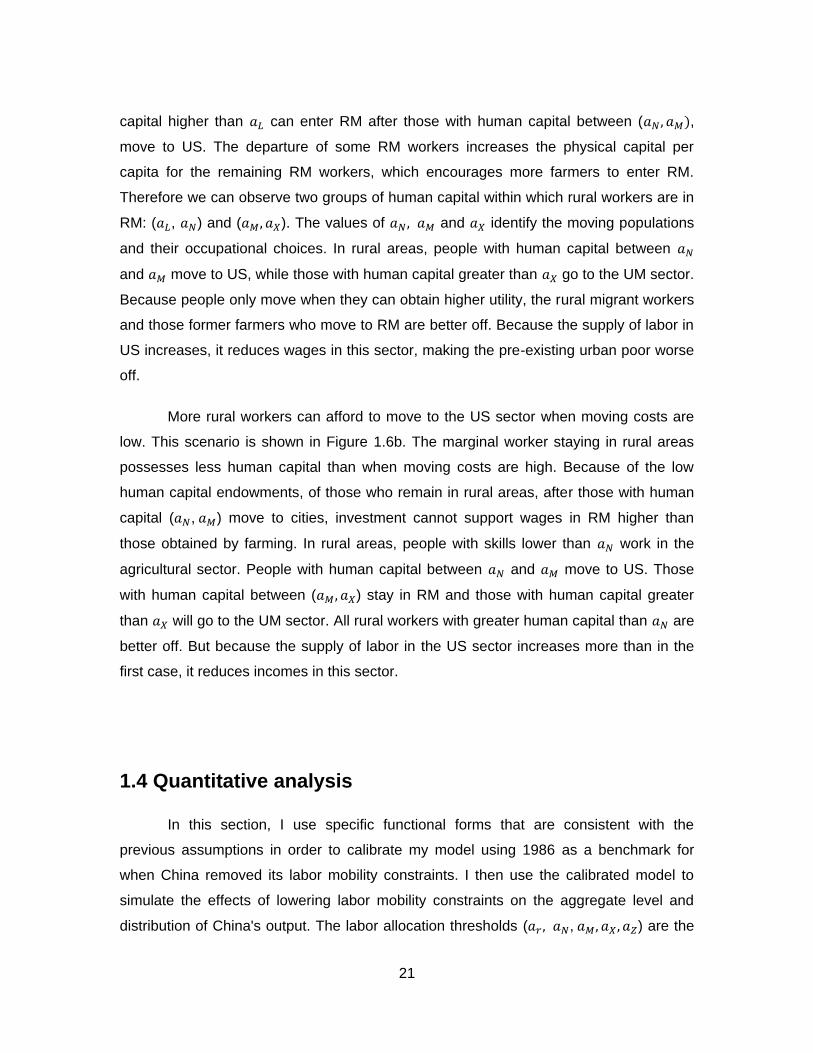
21
capital higher than can enter RM after those with human capital between ( ),
move to US. The departure of some RM workers increases the physical capital per
capita for the remaining RM workers, which encourages more farmers to enter RM.
Therefore we can observe two groups of human capital within which rural workers are in
RM: ( , ) and ( ). The values of and identify the moving populations
and their occupational choices. In rural areas, people with human capital between
and move to US, while those with human capital greater than go to the UM sector.
Because people only move when they can obtain higher utility, the rural migrant workers
and those former farmers who move to RM are better off. Because the supply of labor in
US increases, it reduces wages in this sector, making the pre-existing urban poor worse
off.
More rural workers can afford to move to the US sector when moving costs are
low. This scenario is shown in Figure 1.6b. The marginal worker staying in rural areas
possesses less human capital than when moving costs are high. Because of the low
human capital endowments, of those who remain in rural areas, after those with human
capital ( , ) move to cities, investment cannot support wages in RM higher than
those obtained by farming. In rural areas, people with skills lower than work in the
agricultural sector. People with human capital between and move to US. Those
with human capital between ( ) stay in RM and those with human capital greater
than will go to the UM sector. All rural workers with greater human capital than are
better off. But because the supply of labor in the US sector increases more than in the
first case, it reduces incomes in this sector.
1.4 Quantitative analysis
In this section, I use specific functional forms that are consistent with the
previous assumptions in order to calibrate my model using 1986 as a benchmark for
when China removed its labor mobility constraints. I then use the calibrated model to
simulate the effects of lowering labor mobility constraints on the aggregate level and
distribution of China's output. The labor allocation thresholds ( , ) are the

22
model's key endogenous variables. The values of free parameters are either based on
observed data ( , , , , , , , ), standardized ( , , ) or derived
from theories which are consistent with the data ( ).
1.4.1 Parameters and functions
In 1986, the urban labor force was 132.92 million, while the rural labor force was
379.90 million. The labor force ratio was 1:2.87. The RA sector employed 304.68 million
workers, which was 60% of total labor force. In urban areas, the industrial sector
employed 68.98 million workers, while non-industrial workers numbered 63.94 million.
The total value of industrial output was 1119.4 billion Yuan, among which rural industry
contributed 238.08 billion Yuan. Total investment in urban areas was 211.945 billion
Yuan, while rural investment was 82.017 billion Yuan. The investment ratio was 2.68. In
1986, the incomes per capita in urban and rural China were 1303.19 and 490.27 Yuan.25
Accordingly, I assume that , , and .26 This
information is summarized in Table 1.4.
Table 1.4. Facts and parameters
Urban sector Rural sector Parameter or fact to match
Labor force 132.92 million 379.90 million ,
Industrial employment
68.98 million 75.22 million UM employs 52% of urban labor force
Non-industrial employment
63.94 million 304.68 million RA employs 60% of total labor force
Investment 211.945 billion 82.017 billion and
Industrial output 881.32 billion 238.08 billion The output ratio is 3.7
Income per capita 1303.19 490.27 The income ratio is 2.66:1
25
The income per capita = (total consumption+savings)/population. Please refer to table 1 in Guo (2004).
26 Because there is no data on China's capital stock across periods, I use investment flow to
approximate capital stock. I understand we need very strong economic assumptions to do this approximation, such as assuming the depreciation rate, δ, is very high close to 1 so as K=I/δ at steady state.

23
I assume human capital in both urban and rural areas follows a triangular
distribution on the domain ( ). The rural distribution peaks at , and the urban
distribution peaks at .27
The manufacturing sector uses a Cobb-Douglas production function:
(1.22)
RM is more labor intensive and has less value-added than UM.28 Moreover Jin
and Du (1997) estimated the productivity of China's rural industry in the 1980s. In 1986,
capital incomes and total wages were 24.50 and 24.18 billion Yuan, thus is roughly
equal to .29 Given a CRTS production function, they are both assumed to be 0.5.
Sharma (2007) estimates a Cobb-Douglas production function along with a time trend to
capture the effect of technological progress after the reforms in 1978 using a
cointegration and Error-Correction modeling framework for the 1952-1998 period. He
found that the output elasticity for labor was about 0.37 under the assumption of
constant returns to scale for all of China. Since rural industry accounted for roughly 1/5
of total industry, and .30 and are free parameters in my
model. Each worker's physical labor, , is normalized to 1 in both sectors.
The relative price function is derived in Appendix 1.A:
(1.23)
27
The pdf of a triangle distribution is triangle shaped and it is ( ) (( )( )) if
and it is ( ) (( )( )) if where is the lower limit, is the upper limit and is the mode.
28 Zen (2002) suggested that China's rural industry is more labor intensive, has a lower added-
value and large bulk. 29
Please refer to Table 3.3 in Jin and Du (1997). 30
The urban capital share is 0.63-(0.5 1/5)=0.53 and the urban labor share is 0.37-(0.5 1/5)=0.27. The ratio is roughly 2.

24
Because in 1986 the ratio between the value of industrial goods and agricultural
goods was about 1.62 in China, I assume .31
The wage in US sector is assumed to be Using data
from 1986 to 2008, I ran a regression of on ( ) and ( ) and have
.32 Accordingly, the wage function is assumed to be:
( )
( ) (1.24)
The production function of RA is:
(1.25)
Total labor incomes of urban and rural areas are:
∫ (1.26)
∫ (1.27)
The values of free parameters are calibrated using the equation system
containing equation (1.6) and (1.14) along with the following four equations.
∫ ( )
(1.28)
∫
(1.29)
(1.30)
(1.31)
31
In 1986, the shares of agriculture and industry were 26.9% and 43.7%. (China Statistical Yearbook 2006)
32 The coefficients of ( ) and ( ) are 1.23 and 0.71 with P-values 1.49E-08 and
8.90E-06. Adjusted R² is 0.9494.

25
Equation (1.28) and (1.29) are matching the facts in China's labor market as
shown in Table 1.4. Equation (1.30) reflects the 1986 output ratio between UM and RM.
Equation (31) reflects income disparity in 1986. Notice, however, we have 9 unknowns,
and , which is more than the number of equations. As
my model is a comparison study between China's urban and rural areas, based on the
results of my experiments I assign the values to rural parameters: and
. 33 Moreover, as the value of doesn't affect the outcomes except and , I
normalize its value to 1. After solving this system of equations, the values of the free
parameters are: and . From the
results, we see that has first-order stochastic dominance over as . Also
UM has better TFP as . They are both consistent with the assumptions.
1.4.2 Restricted labor mobility
Using the above parameter values and functional forms, the equilibrium
outcomes at the time when the labor mobility constraints are removed are shown in
Table 1.5.
Table 1.5. Equilibrium outcomes: restricted labor with career options
0.5741 0.6353 43.095 11.647 32.779 1.0438 0.0649 0.0677 0.1638 72.2 69.16 307.8
In urban areas, workers with human capital higher than 0.5741 enter UM, and the
UM employment is 69.16, which is 52% of urban labor force. In rural areas, workers with
human capital higher than 0.6363 enter RM and the RM employment is 72.2 million. The
RA sector employs 307.8 million, which is 60% of the total labor force. The farmers'
income is 0.0677. As the capital available to every RM worker is 1.136, even the most
33
To standardize the values of and , they must bring about real roots to the equation
system; those real roots and parameters must be consistent with all assumptions; and the values should be simple.

26
efficient worker in RM can only make 0.1066. The wage in the US sector is 0.1638. The
total labor incomes in rural and urban sectors are 26.66 million and 24.82 million
respectively and the labor incomes per capita in rural and urban sectors are 0.0702 and
0.1866 respectively.
1.4.3 Unrestricted labor mobility
Because workers are now free to move between labor markets, all variables are
pooled into one equation system. The moving cost function is assumed to be:
( )
(1.32)
where is the fixed moving cost.34
I compare outcomes with different cost functions to examine the effects of
different ways of changing the moving costs. One way is to change the fixed cost and
the other way is to change the variable cost. In the real world, the former is possible by
directly reducing the head fees on migrant workers; the latter can be done by
denouncing negative reports of living and working environments in urban areas.35 I
substitute the specific functions into the system including equation (1.C10), (1.C11),
(1.C12) and (1.C13). Table 1.6 reports the equilibrium outcomes given different cost
parameters.36
34
The moving cost function has two parts. The second term is used to approximate non-money costs, though "it would be difficult to quantify these costs" (Sjaastad (1962)).
35 Zhao (1999) stated that the costs are "related to the psychological adjustments that have to be
made when changing one's home and work environment..." 36
Because of a lack of data, it is difficult to calibrate and . Zhao (1999) showed that, in 1995,
the explicit migrant costs amount to about 30% of the earnings difference between migrants
and rural nonfarm workers. In my simulations, when and , is 31.2% of
the earnings difference between and .

27
Table 1.6. Equilibrium outcomes: unrestricted labor with career options
0.02, 150 0.6351 0.5594 0.5931 0.6774 58.74 6.63 30.58
0.01, 150 0.6313 0.5499 0.5994 0.6730 62.73 6.20 30.27
0.02, 205 0.6290 0.5531 0.5963 0.6771 60.18 6.49 30.37
0, 0.6111 0.5214 0.6111 0.6654 73.65 5.33 28.95
0.02, 150 0.0906 0.0877 0.0930 0.1062 0.1407 0.1319 0.1319
0.01, 150 0.0971 0.0924 0.1007 0.1130 0.1377 0.1292 0.1292
0.02, 205 0.0935 0.0887 0.0957 0.1086 0.1393 0.1294 0.1294
0, 0.1198 0.1005 0.1198 0.1305 0.1305 0.1198 0.1198
0.02, 150 1.336 274.62 33.34 111.37 93.64 56.49 15.52
0.01, 150 1.423 270.04 29.08 113.86 100.03 58.06 22.83
0.02, 205 1.372 271.55 31.85 112.98 96.62 56.61 19.98
0, 1.706 250.93 21.33 121.43 119.31 60.76 46.97
I begin with high moving costs . The urban workers with
human capital higher than 0.6351 enter UM, and the rest go to US. In rural areas,
workers are divided into four groups: workers with human capital less than 0.5594 stay
in RA, and its proportion of the total labor force drops from 60% to 53.53%; workers with
human capital between 0.5594 and 0.5931 move to the US sector; rural workers with
human capital between 0.5931 and 0.6774 stay in RM; while workers with human capital
greater than 0.6774 move to UM. The migration flows to UM and US are 56.49 million
and 15.52 million, respectively. US wage is 0.1319 while the wages in RM range from
0.0930 to 0.1062.

28
The two ways of decreasing moving cost yield different results.37 In the case of
changing the fixed moving cost, drops to 0.01, while remains at 150. This
stimulates migration flows to UM and US, which increase by 2.7% and 47.14%
respectively. The US workers are worse off, since the US wage decreases by 2.05% to
0.1292. In the case of changing the variable moving cost, changes to 205 while
remains at 0.02. This affects the migrations to UM and US to differently: the migration
flow to UM increases very little (by 0.23% to 56.62), while the migration flow to US
increases significantly (by 28.79% to 27.22). The effect on depends on the migration
flows to both UM and US: the migration of workers to UM pushes urban workers out of
UM, but migration to US decreases the wage, thus inducing more urban workers to go
back to UM. In my simulations, the first effect is dominant, so that more urban workers
join US as decreases from 0.6351 to 0.6313 and to 0.6290. When the fixed moving
cost decreases, rural workers with equal to 0.5499 earn 0.0972 in RA. This is higher
than the wage of workers who enter RM, which is 0.0924. When the variable cost
increases, rural workers with , which is equal to 0.5430, earn 0.0935 in RA. Again, this
is higher than the wage of workers who enter RM at 0.0887. Therefore, no farmers
would move to RM after former RM workers move to urban areas. These two cases are
both equilibrium outcomes.
The last case, with and , implies no moving cost across the
country. In this condition, people with the same amount of human capital would earn the
same wage. If the workers' human capital is not sufficiently high to make the owner enter
the industrial sector, workers will stay in either the RA or US sectors, and wages will be
0.1198 for both. The migration flow to UM is 60.76, which is only slightly higher than that
for the two cases above, while the migration flow to US will increase dramatically to
46.97---more than double that of the other two cases. Therefore, with a decreasing
moving cost we would expect that more rural workers would move to the US sector,
rather than to the UM sector.
37
I control the moving cost so that both ways of decreasing moving cost have the same effects on the median rural worker with human capital of 0.4226.
29
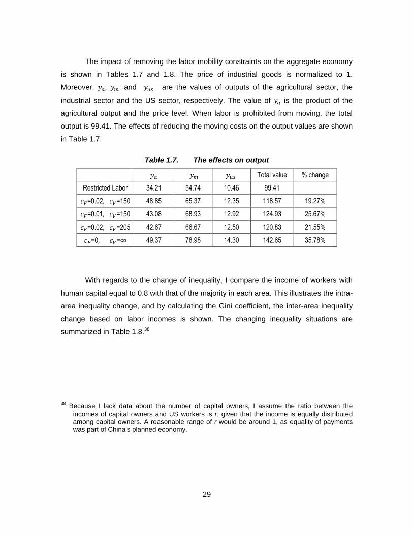
The impact of removing the labor mobility constraints on the aggregate economy
is shown in Tables 1.7 and 1.8. The price of industrial goods is normalized to 1.
Moreover, and are the values of outputs of the agricultural sector, the
industrial sector and the US sector, respectively. The value of is the product of the
agricultural output and the price level. When labor is prohibited from moving, the total
output is 99.41. The effects of reducing the moving costs on the output values are shown
in Table 1.7.
Table 1.7. The effects on output
Total value % change
Restricted Labor 34.21 54.74 10.46 99.41
=0.02 =150 48.85 65.37 12.35 118.57 19.27%
=0.01 =150 43.08 68.93 12.92 124.93 25.67%
=0.02 =205 42.67 66.67 12.50 120.83 21.55%
=0 = 49.37 78.98 14.30 142.65 35.78%
With regards to the change of inequality, I compare the income of workers with
human capital equal to 0.8 with that of the majority in each area. This illustrates the intra-
area inequality change, and by calculating the Gini coefficient, the inter-area inequality
change based on labor incomes is shown. The changing inequality situations are
summarized in Table 1.8.38
38
Because I lack data about the number of capital owners, I assume the ratio between the incomes of capital owners and US workers is r, given that the income is equally distributed among capital owners. A reasonable range of r would be around 1, as equality of payments was part of China's planned economy.

30
Table 1.8. The effects of removing labor constraint on inequalities
Rural inequality change Urban inequality change Gini
Income =0..8 farmer ratio capital US worker ratio
Restricted Labor 0.0853 0.0677 1.26 28.73 0.1638 r 0.2871
=0.02 =150 0.1662 0.0906 1.83 39.16 0.1319 1.69r 0.1344
=0.01 =150 0.1637 0.0972 1.68 41.82 0.1292 1.85r 0.1127
=0.02 =205 0.1646 0.0935 1.76 40.11 0.1294 1.77r 0.1136
=0 = 0.1569 0.1198 1.31 49.10 0.1198 2.34r 0.0463
In rural areas, when labor is immobile, workers with earns 1.26 times
more than farmers. After labor becomes mobile, when and the rural
workers move to UM and the gap increases to 1.83. In urban areas, when labor is
immobile, workers with earns 1.39 times more than the US workers. After labor
becomes mobile, the gap decreases to 1.26. The inequality seems to be better in urban
areas. This result changes when we consider the capital owners' income. The total
income of capital owners, when labor is immobile, is 28.73, but after labor is free to
move their incomes rise dramatically to 39.16. The gap between incomes is thus 1.69
times wider, which is the main reason for the inequality increase in urban areas.
Although we observe higher inequality within both rural and urban areas after labor
becomes mobile, the overall situation is better in terms of labor income. The Gini
coefficient, based only on labor income, was 0.2871 with labor restrictions, while the
value decreased to 0.1344, 0.1127, 0.1136 and 0.0463, respectively. This suggests that
labor income is not the main reason for social inequality in China.
Because and approximate the moving costs in 1995, Table
1.9 compares the model output and data for the same year.39 Moreover, the table
39
To be consistent with the parameter in 1986, when computing , income per capita = (total consumption + savings)/population. The data on migration is from the first agricultural census conducted in 1996.

31
compares the first order difference between 1986 and 1995, indicating the contribution
made by lowering labor mobility constraints to the changes in China's economy.
Table 1.9. Comparison between the model and data
1. (
) 2. . (
) 3. . (
) 4.
5.
Model -7.4% 0.3% 7.1% 21.3% 1.36
Data -8.0% 1.1% 6.9% 12.9% 1.28
6.
7.
8.
9.
10. Gini
Model 34.74% 55.59% 9.67% 1.47 0.1127
Data 8.85% 76.30% 14.85% 3.34 0.4169
Because output of the US sector is measured by industrial goods, I adjust the
data by applying the industry price index to the service sector. Model predictions for the
labor market are close to the data, except for the prediction of a higher migration rate
(21.3%). Model predictions for output changes are slightly different from the data.
Besides the significant changes in labor force, capital investment, technology, and many
other fundamentals that are beyond my static model, have also changed. Another
important explanation for the difference is the price scissors used by China's government
to manually set relatively lower prices for agricultural goods.40 Although no well-accepted
measurement is available for the distorted relative prices in China, the data indicate that
relative prices increased by 59% from 1978 to 1990. Given that the effect of price
scissors persists in China, it would be reasonable to assume that the relative price was
less than 40% of the market price at the beginning of economic reform. If 40% is
accurate, the model outputs of 6, 7, and 8 in Table 9 are 17.56%, 70.23% and 12.21%,
respectively. If the relative price was 20%, model outputs become 9.62%, 76.99% and
13.39%, respectively, which are very close to the data. Moreover, we can see that the
urban-rural labor income disparity shrinks in my model, while in the real world the gap
40
Please refer to Lin and Yu (2009) for more information about the evolution of price scissors in China.

32
between income of urban residents and rural residents becomes wider. By looking at the
Gini coefficient, we can also conclude that the labor-income gap between the two areas
is smaller after the labor market opens, and thus labor income is not the main source of
social inequality. Many economists have tried to explain the urban-rural income disparity
from different perspectives. For example, Yang (1999) argues that "urban biased policies
and institutions, including labor mobility restrictions, welfare systems, and financial
policies of inflation subsidies and investment credits to the urban sector, are responsible
for the long-term rural-urban divide and the recent increases in disparity".
1.4.4 Welfare Change
After removing the labor mobility constraint, a redistribution of the labor force
occurs in both rural and urban areas, as shown in Figure 1.7. Table 1.10 shows the
effects of removing the labor mobility constraint on incomes of rural workers and urban
workers. The moving costs are assumed to be and , the same as in
Table 1.9.
Figure 1.7. Career distributions before and after the labor
mobility constraint is removed

33
Table 1.10. Welfare change after the labor mobility constraint is removed
Rural workers human capital
(millions of workers, % in local labor force)
0-0.5499
(270.04, 71.06%)
0.5499-0.5993
(22.83, 6.01%)
0.5993-0.6353
(14.93, 3.93%)
0.6353-0.6730
(14.15, 3.72%)
0.6730-1
(58.05, 15.28%)
Before 0.0677 0.0677 0.0677 0.0677-0.0717 0. 0717-0.1066
After 0.0972 0.0972-0.1007 0.1007-0.1067 0.1067-0.1130 0.1130-0.1880
% Δ 43.52 43.52-48.67 48.67-57.59 57.59 57.59-76.40
Urban workers human capital
(millions of workers, % in local labor force)
0-0.5741
(63.84, 48.00%)
0.5741-0.6313
(13.36, 10.05%)
0.6313-1
(55.80, 41.96%)
Before 0.1638 0.1638-0.1802 0.1802-0.2854
After 0.1292 0.1292 0.1292-0.2047
% Δ -21.12 (-28.27)-(-21.12) -28.27
Table 1.10 shows the positive effects of the free labor market on the welfare of
rural workers, and the negative effects on the welfare of urban workers. Even though all
urban workers are hurt by the removal of the labor mobility constraint, rural workers gain
far more than the urban workers' losses. Farmers gain the least if they stay in RA. The
rural workers who move to the UM sector gain the most, and the previous urban UM
workers are hurt the most.
1.5 Policy implication
The removal of the labor mobility constraints would help China's economic
growth at the cost of inequality. If the government aims to balance the trade-off between
economic growth and inequality, it must determine the optimal labor mobility constraints
for rural workers. From my calibrations, removal of the labor mobility constraints would
have positive effects on the development of the whole economy, though the effects

34
would be very uneven. Low moving constraints allow more rural workers to move to the
urban sectors, thus hurting the RA outputs. The urban sectors would expand after the
moving barrier is lowered, but the urban workers would be worse off because both
and would decrease. Even though a low barrier of moving would hurt the rural
sectors, it would benefit the rural workers. Moreover, the overall inequality would be
better off in terms of wage incomes. Removal of labor mobility constraints would help the
development of the whole economy, and the decreasing gap between urban and rural
workers' incomes would come at the cost of the urban workers' living standards.
The government can use policies to affect different components of the moving
cost. The fixed cost could be changed by directly reducing the head fees on migrant
workers, or directly subsidizing their transportation costs or accommodation costs, etc.
The variable cost could be increased by denouncing negative reports of the living and
working conditions in urban areas, which are more related to the "psychological
adjustments". The different ways of changing the moving costs would have different
effects on the economy, because a uniform extra moving cost would have a stronger
negative effect on all types of rural workers, compared to changing the variable cost,
which would have a greater effect on the low-ability rural workers. The increased
negative effect on all types of rural workers would have a negative impact on both types
of migration flows, while the greater effect on the less efficient rural workers would have
stronger effect on flow to US than to UM. Even though both ways of changing the
moving costs would lead to changes in the total economy, the decrease in fixed cost
would lead to a greater increase. Since both ways have similar effects on inequality,
controlling the fixed moving cost would be better, in terms of developing the real sectors.
Another advantage of controlling the fixed moving cost is from its precision as a result of
being measurable, unlike the variable moving cost which is difficult to accurately
quantify.

35
Because China still had 36 million rural poor population by 2010, how to help
them out of poverty is very important for China's economic development.41 Although my
model results suggest that rural workers are better off with the removing of labor mobility
constraints, the outputs of rural sectors are hurt, given the same investment profile. It
implies that the increase in rural incomes comes mainly from the expansion of the urban
sectors. This increase is vulnerable to the constraints on labor mobility. Therefore, how
can we help the rural poor and shrink the gap between the rural and urban areas
sustainably?
Investing more in rural education is crucial for changing the distribution of human
capital in the rural population. With better education, more rural people would be
qualified for industrial positions, which would stimulate the rural economy and income
per capita. Still, much time would be needed to see an effect. Another, more efficient
way to affect rural growth is to directly and constantly increase investment in the RM
sector. This would increase the demand for rural workers and increase their incomes.
Moreover, as shown in my model, the US sector is a channel for redistributing total
social wealth, implying that a more complete service business should be developed in
both rural and urban areas to make the channel smoother. More rural workers with low
human capital should be involved in developing the rural service (RS) sector. Typically,
the transfer of most production lines to rural areas would take advantage of the low labor
cost. To help more of the rural poor in the agricultural sector, more advanced
technologies must be introduced to increase MPN, or a large amount of labor must be
released from the agricultural sector. The released labor can then be absorbed either
domestically or internationally. Domestically, labor-intensive industries could be
encouraged, such as the hand-made craft sector that requires no/low physical
investment. Furthermore, the government could remove some rural people from the rural
economy, for example, by recruiting more soldiers from the rural areas. Internationally,
the government should actively contact countries that have a shortage of labor and
41
The number is quoted from China's Human Resource, by State Council Information Office of PRC.

36
export labor to them, since the labor export would give domestic workers more job
opportunities.
1.6 Conclusion
This paper develops a model with heterogeneous agents, endogenous internal
migration, and endogenous labor markets, and calibrates it to analyze the effects of a
key component of China's recent economic reform, namely, the gradual removal of
internal labor mobility constraints, on its economic development and inequality issues
within the country's urban and rural areas. Because China's government adopted an
urban-biased investment strategy, investment decisions are assumed to be exogenous
in the model. This paper primarily focuses on intra-regional inequality. The model
features heterogeneous workers who look for jobs in two regions (urban and rural areas)
and across four sectors (urban modern industrial sector (UM), urban subsistence sector
(US), rural modern industrial sector (RM), and rural traditional agricultural sector (RA)).
In equilibrium, high-ability rural workers go to the UM sector, while workers who stay in
the RM sector may come from two discontinuous groups. All workers who are between
the two groups have an incentive to move to the US sector after the legal labor mobility
constraints are removed. The heterogeneity of labor increases inequality in both rural
and urban regions, even though many rural residents are better off than before.
Calibrations show the positive contribution from allowing domestic migration on
developing the whole economy, even though the effects are very uneven. The
calibrations also suggest an enhancement of inequality within both rural and urban
areas. Among the various ways of helping the rural poor, investing more in education,
increasing capital investment in rural areas, developing the RS sector, and finding other
channels to absorb the abundant rural labor force would all be suitable strategies for
promoting the sustainable growth of China's rural economy.
Although most stylized facts related to China's internal migration can be
explained from my model, it has several weaknesses that point to possible extensions in
future research. Firstly, the economy in my model is assumed to fully follow market

37
principles. In the real world, however, China is still transitioning from a planned economy
to a market economy, though it has already changed from a closed economy to a large
open economy during the process of marketization.42 For example, my model does not
capture the price distortion occurring at the beginning of China's economic reform or
some features of an open economy.43 Second, my model is static, while in reality people
think not only about their current benefits but also about their future welfare. Also, this
static model cannot explain the urban-rural inequality change. Third, though I mention
that human capital can be influenced by education and job training, I do not assume
options for the agents to accumulate human capital. Because urban areas have better
education resources, another incentive is present for rural workers to move. Such issues
are studied in Lucas (2004). Fourth, since no unemployment is present, no uncertainty
exists in my model, which is not entirely consistent with the actual China's economy.
Many economists have presented reasons for unemployment. For example, Harris and
Todaro (1970) proposed a random job selection process over an excess labor supply;
Cooper (1985) studied involuntary unemployment from asymmetric information; and
Andolfatto (2008) analyzed unemployment by using a search model. These authors all
provide good hints on how to incorporate unemployment into the present model.
42
China began its economic reform in 1979 and declared its market economy in 1992. As of February 2008, China's market economy status has not yet been recognized by the US or the EU, though it has been recognized by 77 other countries.
43 The price scissors between industrial goods and agricultural goods existed in China until 1992
when the country declared itself as a market economy. See Lin and Yu(2009).

38
1.7 References
Andofatto, D., 2008. Search Models of Unemployment. The New Palgrave Dictionary of Economics, 2nd edition.
Au, C., Henderson, J., 2006. How Migration Restrictions Limit Agglomeration and Productivity in China. Journal of Development Economics. 80(2), 350--388.
Borjas, G., 1987. Self-Selection and the Earnings of Immigrants. The American Economic Review. 77, 531--553.
Cheng, Y., 2007. The Evolution of China's Gini Coefficient and Its Decomposition Between Urban and Rural Areas After Economic Reform (in Chinese: Gaige Yilai Chengxiang Zhongti Gini Xishu de Yanbian Jiqi Chengxiang Fenjie). China's Social Science (Zhongguo Shehui Kexue). 4.
Cole, W., Sanders, R., 1985. Internal Migration and Urban Employment in the Third World. The American Economic Review, 75(3), 481--494.
Cooper, R., 1985. Worker Asymmetric Information and Involuntary Unemployment. Journal of Labor Economics. 3(2), 188--208.
Du, Y., Park, A., Wang, S., 2005. Migration and Rural Poverty in China. Journal of Comparative Economics. 33, 688--709.
Guo, X., 2004. A New Estimation of the Income Gap Between Rural and Urban Areas (in Chinese: Chenxiang Shouru Chaju de Xinguji). Shanghai Economic Study (Shanghai Jinji Yanjiu). 12.
Harris, J., Todaro, M., 1970. Migration, Unemployment and Development: A Two-sector Analysis. The American Economic Review. 60(1), 126--142.
Jin, H., Du, Z., 1997. Productivity of China's Rural Industry in the 1980's. Chinese Economics Research Center (CERC) working papers. 1997-06.
Kung, J., Lin, Y., 2007. The Decline of Township-and-village Enterprises in China's Economic Transition. World Development. 35(4), 569--584.
Krusekopf, C., 2002. Diversity in Land-tenure Arrangements Under the Household Responsibility System In China. China Economic Review. 13, 297--312.
Lin, J., Yu, M., 2009. The Political Economic Analysis of China's Price Scissors: Theory Model and Empirical Evidence (in Chinese: Wogou Jiage Jiandaocha de Zhengzhi Jingjixue Fenxi: Lilun Moxin Yu Jiliang Shizheng). Economic Study (Jingji Yanjiu), 1, 422--456.
Lu, Y., 2002. China's Hukou System After 1949: Structure and Evolution (in Chinese: 1949 Nian Hou De Zhonggou Huji Zhidu: Jiegou Yu Bianqian). Jounal of Peking University (Beijing Daxue Xuebao). 2.

39
Lucas, R., 2004. Life Earnings and Rural-Urban Migration. Journal of Political Economy. 112(1), S29--S59.
Naughton, B., 2007. The Chinese Economy: Transitions and Growth. MIT Press. Cambridge.
Pan, X., Sun, G., 2008. A Survey and Analysis on the Education of the Children of Migrant Workers (in Chinese: Jincheng Mingong Zinu Jiating Jiaoyu De Diaocha Yu Fenxi). Journal of the Party School of CPC Hangzhou (Zhonggong Hangzhou Shiwei Dangxiao Xuebao). 4.
Ravallion, M., and Chen, S., 2007. China's (uneven) progress against poverty. Journal of Development Economics. 82, 1--42.
Roy, A.D., 1951. Some Thoughts on the Distribution of Earnings. Oxford Economic Papers. 3, 1352--146.
Sharma, H., 2007. Sources of Economic Growth in China, 1952-1998. Issues in Political Economy, 17.
Shoven, J., and Whalley, J. 1992. Applying General Equilibrium. Cambridge University Press.
Sjaastad, L., 1962. The Costs and Returns of Human Migration. The Journal of Political Economy. 70(5), 80--93.
Wang, F., Zuo, X., 1999. Inside China's Cities: Institutional Barriers and Opportunities for Urban Migrants. The American Economic Review. 89, 276--280.
Whalley, J., Zhang, S., 2007. A Numerical Simulation Analysis of (Hukou) Labour Mobility Restrictions in China. Journal of Development Economics. 83, 392--410.
Yang, D., 1999. Urban-Biased Policies and Rising Income Inequality in China. The American Economic Review. 89(2), 306--310
Yao, S., 1994. Agricultural Reforms and Grain Production in Rural China. Palgrave Macmillan.
Zen, F., 2002. On the Interaction of Urbanization and Industry Structure (in Chinese: Lun Chengshihua Yu Chanye Jiegou De Hudong Guanxi). Economic Review (Jingji Zhongheng), 10.
Zhang, K., Song, S., 2003. Rural--urban Migration and Urbanization in China: Evidence from time-series and cross-section analyses. China Economic Review. 14, 386--400.
Zhao, Y., 1999. Labor Migration and Earnings Differences: The Case of Rural China. Economic Development and Cultural Change. 47(4), 767--782.

40
Zhang, W., Lei, K., 2008. The Analysis of the Structure, Status Quo and Determinants of a New Urban Migrant's Social Integration (in Chinese: Chengshi Xinyimin Shehui Ronghe). Sociology Study (Shehuixue Yanjiu). 5.
1.8 Appendices
Appendix 1.A: relative price formation
Assume the homogeneous utility function over agricultural and industrial goods is:
( )
(1.A1)
With different income levels and a normalized price of industrial goods, the optimal
consumption of each person is:
(1.A2)
(1.A3)
We have:
(1.A4)
To clear the market, /
must equal / which gives us:
(
) (1.A5)
Generalizing it I assume the relative price forming function as equation 1.4.
Appendix 1.B: mathematical equilibrium in figure 1.6
Mathematically, employment levels in the urban sectors, and are defined as:
∫ ( )
∫ ( )
(1.B1)

41
∫ ( )
∫ ( )
(1.B2)
Because some previous farmers would move to RM, the employment levels in rural areas now
change. Now a farmer with human capital is indifferent between working in RA or RM, and the
employment levels in RA and RM are:
∫ ( )
(1.B3)
∫ ( )
∫ ( )
(1.B4)
The relative price, , is defined as:
(
) (1.B5)
where , and are defined as:
( ) (1.B6)
∫ (
)
∫ (
)
(1.B7)
∫ (
)
∫ (
) ( )
(1.B8)
At equilibrium, the rural worker with must be indifferent between farming and working in RM;
that is:
(
) ( ) (1.B9)
For the rural worker with who is indifferent between working in RM and US:
(
) ( ) ( ) (1.B10)
For the rural worker with who is indifferent between working in RM and US:
(
) ( ) ( ) (1.B11)
For the rural worker with who is indifferent between working in RM and UM:

42
(
)
(
) ( ) (1.B12)
For the urban worker with who is indifferent between working in US and UM:
( )
(
) (1.B13)
With the expression of P which is shown in equation B5, the equation system with equation B9,
B10, B11, B12 and B13 determines the values of , , , . To make extra labor enter
RM, at equilibrium the solutions must satisfy:
(
) ( ) (1.B14)
Appendix 1.C: mathematical equilibrium in figure 1.6
is the employment in RM:
∫ ( )
(1.C1)
The wage of farmers is:
( ) (1.C2)
where P is the relative price which is determined by:
(
) (1.C3)
where , , and are the equilibrium outputs of RA, RM and UM sectors, which are defined
in equation 1.C7, 1.C8, and 1.C9.
The employment levels of RA, US and UM are:
∫ ( )
(1.C4)
∫ ( )
∫ ( )
(1.C5)
∫ ( )
∫ ( )
(1.C6)

43
The outputs of RA, RM and UM are:
( ) (1.C7)
∫ (
)
(1.C8)
∫ (
)
∫ (
) ( )
(1.C9)
The rural worker with must be indifferent between working in agricultural and US; that is:
( ) ( ) ( ) (1.C10)
The rural worker with must be indifferent between working in RM and US; that is:
(
) ( ) ( ) (1.C11)
The rural worker with must be indifferent between working in RM and UM; that is:
(
)
(
) ( ) (1.C12)
The urban worker with must be indifferent between working in US and UM; that is:
( ) (
) (1.C13)
Because my employment functions and output functions are all of , , and , the
equilibrium values are determined by solving the equation system containing 1.C10, 1.C11,
1.C12, and 1.C13. To make no extra labor enter RM, at equilibrium the solutions must satisfy:
(
) ( ) (1.C14)

44
Chapter 2. The Economic Effects of Minimum Wage Policy
2.1 Introduction
Nowadays minimum wage policy has been popularly used in both developed and
developing countries, even though it serves different purposes. As pointed out by
Watanabe (1976), developed countries intend to use minimum wages to provide an
acceptable living standard for their marginal workers, while developing countries intend
to use minimum wages to adjust their social inequalities. It is commonly agreed that
minimum wages increase unemployment and reduce output when workers are
homogenous and labor markets are perfectly competitive in the presence of perfect
information. Absent these restrictive assumptions, however, many economists draw
different conclusions. For example, some have shown that minimum wages might be
Pareto optimal if the labor market is not competitive (Boal & Ransom (1997), Strobl &
Walsh (2007), and Ashenfelter, Farber & Ransom (2010) have shown that minimum
wages decrease unemployment in a monopsony market); if workers are not
homogeneous (Drazen (1986) suggested that, with heterogeneous workers, minimum
wage may be Pareto optimal if a higher wage would be preferred to the market clearing
wage, even though unemployment is produced); and if there is no perfect information
(Broadway & Cuff (2001) argued that minimum wage may be optimal because it can be
combined with the institutional features of a typical welfare system to fix the
government's asymmetric information problem with respect to workers' abilities).
In this paper, I study the effects of minimum wages on a transitional economy,
such as China, in which migration flows from rural to urban areas occur with positive
moving costs. There are three main results from my analysis. First, minimum wage is a
useful instrument for the government to control migration flows. Second, regarding social
inequality adjustments, a minimum wage leads to improvements in urban areas, but to a

45
worsening in both rural areas and the country as a whole. Third, a minimum wage may
be optimal due to the moving friction: a moving cost wedge induces a modestly binding
minimum wage to cause relatively low productivity urban workers to be replaced by
higher productivity rural migrants. To show these results, I construct a theoretical model,
focusing on the selection effects on determining the labor market outcomes, and then
compare the outcomes with minimum wages to the status quo ante. Theory indicates
that minimum wage policy has different effects on migration flows to formal sector,
depending on the level at which it is set. When its value is low, minimum wage induces
fewer urban workers but more migrant workers to work in the urban modern industrial
sector. However, when its value is high, migrant workers are also constrained from
entering the urban industrial sector. The effects on the urban informal sector are unclear.
I then calibrate my theoretical model by using data from China to simulate the effects of
minimum wages. I begin by calibrating my model's parameters to match labor market
outcomes in China in 2006. By using 2006 as benchmark, the calibrated model predicts
that when the minimum wage is not high enough to constrain qualified rural workers from
moving to the urban industry sector, it benefits the whole economy; otherwise, it has
negative effects on economic growth. The calibration also predicts worse inequality in
rural areas but less inequality in urban areas, given the same investment profile. To
achieve the second best outcome, government shall fully compensate the moving costs
for the marginal migrant workers from the rural industrial sector to the urban subsistence
sector, and the minimum wage shall not be binding for migrant workers in the urban
industrial sector.
A minimum-wage system was officially introduced in China's Labor Law in 1994.
It stated that the minimum wage should be set to ensure that the lowest wage earned by
a worker be sufficient to support her basic needs. The Labor Law was an attempt to
protect workers by specifying the form of payment, maximum hours, and overtime rates.
In reality, it functioned more like a set of recommendations than binding policy, because
there was no solid punishment for firms that did not abide by it. Although the minimum
wage increased several times after 1994, the average income of low-skilled workers fell
further behind the average urban income. Between 1994 and 2004, the average annual
income of civil servants in Dongguan City increased by as much as 340%, from 8,000
RMB to more than 35,000 RMB; during the same period, average wages in the leather

46
and shoe industry stayed between 6,000 RMB to 10,000 RMB, and only increased by a
total of 71%.44 The Provisions on Minimum Wages was enacted in 2003 by the Ministry
of Labor and Social Security, as an attempt to strengthen the protection of low-skill
workers provided by the minimum-wage system. It required that the minimum wage be
readjusted at least every two years according to such factors as the cost of basic
necessities for employees and their dependents, as well as the local consumer price
index. The readjustment was frozen in 2009 due to the worldwide recession. In 2010,
following the recovery of China's economy and due to shortages of migrant workers, 30
of China's 31 provinces and direct-controlled municipalities announced increases in their
minimum wages, at different rates. For example, Shanghai has China's highest minimum
wage at 1120 RMB per month---an increase of 16.7%; in Guangdong province it
increased by 21.1%; Hainan province saw the greatest increase at 37%.45 But these
wages are still very low when compared with the local average wage. For example, the
average wage in Shanghai was 3759 RMB in 2009, while its minimum wage in 2010 was
only 30% of that.46
This paper analyzes the effects of minimum wage policy by using China as an
example. Followed by the introduction, the rest of this paper is organized as follows.
Section 2.2 contains the basic model setup and analysis. Section 2.3 analyzes the
effects of minimum wage policy. Section 2.4 provides calibrations and simulations of my
model. Section 2.5 discusses some potential policy implications. Section 2.6 concludes,
and suggests some potential extensions.
44
More information can be found in Wages in China, published on China Labor Bulletin on Feb 19th, 2008
45 The information is published on the official website of The Central People's Government of The
People's Republic of China. 46
Numbers are quoted from the Shanghai Statistical Yearbook 2010

47
2.2 Model setup
2.2.1 Model assumptions
I construct a model with two regions, rural and urban, and four sectors to
facilitate internal migration. Each region has two sectors. Rural areas possess a
traditional agricultural (RA) sector and a modern industrial (RM) sector. Urban areas
possess a former urban modern industrial (UM) sector and an informal urban
subsistence (US) sector. The RM sector is developed with some exogenous physical
capital investment, which is significantly less than is invested in urban areas. All
residents can be identified by a residency registration system. The rural labor force is ,
and the urban labor force is , and I assume that is much greater than . I also
assume that each worker possesses some human capital.47 Initial levels of human
capital are determined by nature, while education and job-training yield significant
increases. Each worker has his own human capital, which ranges from 0 to 1. The
distributions of human capital in the rural and urban populations are and ,
respectively. Since education resources are allocated more in urban areas and there are
uneven opportunities to access to post-secondary education, is assumed to exhibit
first-order stochastic dominance over .
In the RA sector, labor is considered homogenous, and the production function
is:
( ) (2.1)
where is total physical labor input. I assume . Farmers are paid at their
marginal product of labor (MPNs) and the government, as the landowner, takes all the
remaining output.
47
Here human capital is defined as the stock of skill and knowledge embodied in the ability to perform labor, so it can be measured in terms of productivity.

48
In the industrial sectors, I assume agents work individually and the produce
functions are CRTS. Workers are paid their marginal product. Each worker's production
function in UM and RM are:
( ) (2.2)
( ) (2.3)
where is the human capital possessed by worker , and is the physical labor input of
each worker, which is normalized to 1. Note that I assume total capital investment in
both industrial sectors is equally distributed among the workers, and
. The marginal product of labor, , is increasing with and as capital
and labor are complements. Government allocation of investment between sectors is
assumed to be exogenous and . Manufactured goods are homogeneous.
The relative price between agricultural goods and industrial goods, P, clears
the market. Manufactured goods are defined as the numeraire. The price function is:
(
) (2.4)
with ( ) .48
2.2.2 The best outcomes
The first best outcome occurs when all resources are mobile across sectors, and
there is thus no difference between urban and rural areas. In the first best case, capital
goes to the sector with higher returns between industrial sector and agricultural sector.
48
One possible way to endogenize it is to assume homogeneous preference over both agricultural and industrial goods (e.g. Cobb-Douglas). Given a relative price level, the consumption ratio is constant, and should be proportional to the ratio of outputs when the market clears. Thus relative price is negatively related to the ratio of outputs. Please refer to Appendix 2.A.

49
There is a boundary of human capital in that those workers with higher human capital
work in the manufacturing sector and those with lower human capital work in the
agricultural sector. Since in my model labor is the only flexible factor and there are many
practical constraints, the first best case is not possible in the real world at least in the
near future, and thus it will not be discussed in detail.
The second best outcome occurs with only one constraint: that is, capital is
predetermined. In the second best case, the difference between urban and rural areas
exists since investment profiles are quite different. To induce the second best outcome,
the moving costs must be assumed away. If the US sector is assumed to be a channel
to reallocate social wealth and produce no real outputs, and the utility functions are
based on real outputs only, the second best outcome must satisfy several conditions.
First, agents' utilities are maximized given the outputs of manufactured goods and
agricultural goods. Second, workers with the same human capital are treated equally.
That is, either they are all in the same sector or they are all out of that sector, since labor
is totally mobile. Third, in the second best outcome the marginal products of labor for the
same worker must be equalized across UM and RM sectors, which determines the labor
allocation. This may imply an urban-to-rural migration flow to the RM sector if it requires
more workers.
Based on my model setup, the second best outcome may be derived in a simple
way. Because of the properties of the production functions in modern industry sectors,
there are two opposite effects when an extra worker enters. On the one hand, labor
increases, contributing positively to total outputs. On the other hand, the extra workers
decrease the capital available to each worker, which has a negative effect on output.
Therefore the total output may be maximized at a certain cut-off level of human capital.
At this cut-off level of human capital, once the ratio between manufacturing goods and
agricultural goods exceeds the optimal ratio of subjective demands which is determined
by equating the marginal utilities of consuming each good, some workers must switch
from the industrial sector to the agricultural sector until the output ratio is optimal.
Otherwise, the second-best outcome is induced. Numerical analysis cannot be done
without specific assumptions on functional forms. I discuss this further in Section 2.4.

50
The equilibrium outcome that we may observe in the real world is the market
equilibrium. Besides the constraint imposed on the second best case, the market
equilibrium also experiences positive moving costs. This is the main focus of this paper.
2.2.3 The market equilibrium outcome
To determine the market equilibrium outcome, moving costs must be considered
since migrant workers are subject to them in the real world. The costs of moving to big
cities are not just pecuniary, but also include psychological discomfort, such as
loneliness, discrimination from urban residents, safety issues, etc. 49 Assuming high-
skilled people adapt to a new environment faster, the cost of moving is modeled as a
decreasing function of .50 I assume the annuitized cost of moving is is ( ) with
( ) .51
When a rural worker considers moving, she compares the benefits of moving to
the cost. By assuming that a higher wage is the benefit she would earn if working in an
urban area, her net benefit function is:
( ) ( ) ( ) (2.5)
I assume that ( ) ( ) ( ) , i.e.
49
Sjaastad (1962) breaks down the moving cost into money and non-money costs. "The former include the out-of-pocket expenses of movement, while the latter include foregone earnings and the 'psychic' costs of changing one's environment". Zhao (1999) called them "explicit costs" which also include the costs imposed by government and "implicit psychic cost".
50 The moving cost is also affected by the locations of rural areas, traffic conditions, and other
factors, while I focus on the effects of human capital. 51
Zhang and Lei (2008) point out that there are four components in social integration for a Chinese domestic migrant: cultural integration, mental integration, identity integration and economic integration. They also construct an empirical model to test the determinants on social integration by using data on 600 new migrants to Shanghai. The coefficient of schooling years is 0.89 which implies migrants with higher education levels integrate into a new society faster.

51
( ( ∫
)) ( )
( ( ∫
)) (2.6)
to make sure that at least the highest ability rural worker obtains a net benefit from
moving to the UM sector. Because working in UM yields higher wages, rural workers
consider their qualifications for positions in this sector first, given the same moving cost,
if they decide to move. Employment in the urban industrial sector is now composed of
urban workers and migrant rural workers.
Proposition 2.1: The migration flow to the UM sector is inversely related to the
moving costs.
Proof. The rural worker moving to UM with the least human capital, , must be
indifferent between the benefits from staying in the rural sector and the wages earned in
the UM sector. Employment in the UM sector includes urban workers and migrant
workers which are:
∫ ( )
(2.7)
∫ ( )
(2.8)
where is the least human capital possessed by an urban worker who stays in UM. A
migrant worker from rural areas with must satisfy:
( ) (2.9)
where is the income of the rural migrant worker with who moves to UM which
equals ( ( )) and is the income of the same worker who
stays in RM which is ( ) and is the employment in RM:
∫ ( )
(2.10)

52
where is the least human capital possessed by a rural worker who stays in RM. We
know that ( ) and ( ) thus the RHS of equation (2.9) is a decreasing
function on . In LHS:
( )
( )
( )
( )
where ( ) and all terms are positive which implies is an
increasing function of .
( )
( )
( )
( )
where . We have and
as positive terms but ( )/ ( ) is
negative. Therefore may increase or decrease with . But as UM is assumed to
always be attractive to high ability workers, increases slower than
}. Therefore
the LHS of equation (2.9) is an increasing function of . Figure 2.1 depicts the
information embodied in equation (2.9).
Figure 2.1. Equilibrium human capital thresholds

53
Intuitively, institutional and economic barriers increase the cost of moving, and
local job options faced by rural workers increase the benefit of staying. Therefore, they
work in the same direction on labor mobility. The equilibrium human capital of the last
rural worker who would move to UM is , where
intersects ( ). If labor
mobility across areas was allowed without setting up RM, is determined by
( ) which ends up at lower .52 More rural workers would flow into UM. On the
other hand, if the government imposes extra restrictions on the requirements of urban
job positions for rural workers, it pushes up the cost curve to ( ). Consequently more
rural workers would stay in rural areas. Therefore, the government has multiple tools to
control migration to the UM sector.
Not every job seeker is qualified to have a job in the UM sector. Many of them
have to work in US. As described in Cole and Sanders (1985), US consists of "those
urban employment categories that feature very low levels of productivity and earnings".
US can absorb all labor which wants to work in it, thus there is no unemployment for
migrant workers. This is the key difference from Harris and Todaro (1970). All US
workers are assumed to be paid at . Even though is less than the wage earned
in UM, the fact that people do stay in the city and don't go back indicates that it is still
greater than the potential wage when working in rural areas. The wage difference
provides the incentive for some rural workers to move to cities, even if only to get a
position in US.
Proposition 2.2: There is a lower limit, ( ) and an upper limit, ( )
with , on human capital with which rural workers move to the US sector.
Only the rural workers with human capital between and move to the US
sector.
52
is the wage earned by farmers which is no higher than .

54
Proof. Rural workers heading to the US sector must satisfy the following
condition:
( ) (2.11)
where and ( ) are defined the same as before, and is the wage when staying
in rural areas. It may be the wage from either RA or RM, because either farmer or
worker, or both, may consider moving to US. But because is the lowest wage for the
workers in UM, only those who cannot go to UM will think about going to US.
Because ( ) is a decreasing function of human capital, is a non-decreasing
function of human capital and is the same for every worker in US, Figure 2.2
illustrates the situation in which rural workers would move to US.53
Figure 2.2. Heading to the US sector
Figure 2.2c shows that there exists an upper limit, , and a lower limit, , of
human capital for which rural workers would move to US. It implies we would not
53
The combination of a decreasing function plus a non-decreasing function may bring about another result: overall effect is always decreasing if dominates. The U-shaped curve also
can be very asymmetric if is much flatter than Provided is greater than the minimum point of , these two cases end up with only one intersection. In the first case, all highly skilled rural workers have an incentive to move to US; in the second case, all less smarter rural workers will move to US. These two are not consistent with the data.

55
observe extreme types of rural people in US. Those rural workers with human capital
close to who work in RM, but who are not skilled enough to find a job in UM sector,
they can take advantage of affordable moving costs to earn higher wage in US. On the
other hand, for those rural workers with human capital close to who are paid much
less, the wage in US will be attractive in spite of high moving costs. Figure 2.2c also
indicates that a higher moving cost discourages rural workers from moving to the US
sector, and so we observe more homogeneity among migrant workers in the US sector.
Another application of figure 2.2c is to analyze migration differences between
rural areas. Using China as an example, we know that most of China's developed areas
are located in the eastern and southern coastal regions, while most of its less-developed
areas are located in the central and western regions. Intuitively, the moving cost for a
rural worker from a county close to developed cities is lower than for someone living far
away from them, assuming all other factors are the same---for example, a rural worker
from Anhui province vs. a rural worker from Qinghai province---therefore, given the same
wage earned in urban areas, we would observe less migration from those rural areas
located far away from big cities.
Proposition 2.3: Two different equilibrium scenarios may appear in rural areas
after rural workers move to urban areas. Rural workers with human capital in
excess of move to the US sector. The workers with less human capital than
could enter RM or stay in RA. These two scenarios are depicted in Figure 2.3.

56
Figure 2.3. Career distribution in rural areas
The mathematical conditions for these two scenarios are showed in Appendices
2B and 2C. The intuition is as follows. Fewer rural workers move to the urban US sector
when moving costs are high. This scenario is shown in Figure 2.3 . Figure 2.2c implies
in Figure 2.3 is greater than in Figure 2.3b which has lower moving costs. It
implies a higher wage if the one on the boundary works in RM. This provides room for
rural workers with human capital slightly less than to earn higher wages in RM than
staying in RA after some rural workers move to US. The rural workers with human
capital higher than can enter RM after those with human capital between ( ),
move to US. The departure of some RM workers increases the physical capital per
capita for the remaining RM workers, which encourages more farmers to enter RM.
Therefore we can observe two groups of human capital within which rural workers are in
RM: ( , ) and ( ). The values of and identify the moving populations
and their occupational choices. In rural areas, people with human capital between
and move to US, while those with human capital greater than go to the UM sector.
Because people only move when they can obtain higher utility, the rural migrant workers
and those former farmers who move to RM are better off. Because the supply of labor in
US increases, it reduces wages in this sector, making the pre-existing urban poor worse
off.
More rural workers can afford to move to the US sector when moving costs are
low. This scenario is shown in Figure 2.3b. The marginal worker staying in rural areas
possesses less human capital than when moving costs are high. Because of the low
human capital endowments, of those who remain in rural areas, after those with human
capital ( , ) move to cities, investment cannot support wages in RM higher than
those obtained by farming. In rural areas, people with skills lower than work in the
57
agricultural sector. People with human capital between and move to US. Those
with human capital between ( ) stay in RM and those with human capital greater
than will go to the UM sector. All rural workers with greater human capital than are
better off. But because the supply of labor in the US sector increases more than in the
first case, it reduces incomes in this sector.
2.3 Minimum wage
Workers' moving decisions and the market outcomes with free labor mobility may
be different with government intervention. To avoid a huge migration flow flushing into
cities when the labor mobility constraint is removed, government can use minimum wage
policies to smooth the transition, and to maintain subsistent living standards for low-
income workers. Since it is effective to enforce minimum wage on formal sectors, I
assume that minimum wage is imposed on the UM sector at w. It has significant effects
on the labor market. To begin, we consider the UM workers.
Proposition 2.4: After labor becomes mobile, the minimum wage induces fewer
urban workers to enter UM. The effects on migration to UM depend on the value of
the minimum wage. When is low, it induces more migrant workers to move to
UM, compared to the condition without a minimum wage. When is high, migrant
workers are limited from moving to UM and less migrant workers move to UM.
Proof. We begin by considering the effects of on urban workers. Without any
migrant workers, the UM employment is ∫
. When labor is mobile, total
employment in the UM sector includes urban workers and migrant workers. That is,
∫
where is the least human capital that an urban worker can
have and still stay in UM, and is the number of migrant workers in UM. When

58
the minimum wage is enforced, it determines the least human capital with which the
urban worker could stay in UM. We have:
(
∫
) (2.12)
For any given urban human capital level, the RHS of equation (2.12) is less than
(
∫
), which is the wage of urban UM workers when labor is immobile,
since each worker will have less physical capital to work with. Figure 2.4 shows the
effect of on urban workers.
Figure 2.4. The effects of on urban workers
Because must be greater than , is greater than . Figure 2.4 shows
that when is enforced, the probability of fewer urban workers staying in UM after labor
becomes mobile is higher than in the case without . If drops quickly after labor
becomes mobile, we may observe more urban workers in UM after the labor mobility
constraints are removed.

59
With regard to the rural workers, we know that . Because if not, then
would be the minimum requirement to enter UM in the urban area. Since everyone in
UM has the same amount of capital to work with, the marginal migrant workers with
would earn less than the marginal urban workers with . Because the marginal urban
workers with is indifferent between entering UM and US, their incomes are .
Therefore the marginal migrant workers to UM would earn less than which is
impossible since they would then move to US instead of UM.
There are two scenarios regarding rural workers. If the MPN of marginal movers
when they work in UM is greater than w, their decision is based on:
( ) (2.13)
where is the wage if the worker moves to UM and
is the wage if the
same worker stays in RM. If we keep the same as before, since we expect fewer
urban workers in UM than in the case without , only is affected, and will be
higher than in the case without minimum wage. Therefore, the LHS of equation (2.13)
must be reduced if it is to hold, which implies that more rural workers are moving to UM.
Nevertheless, if , then rural workers whose MPN when working in
UM is lower than w are not accepted by any UM firms, because of the enforcement of
the minimum wage. In this case the MPN of the last worker moving to UM must be at
least equal to . That is:
(2.14)
The higher the minimum wage, the less qualified rural workers need be to move
to UM. Because also equals the MPN of the last urban workers who can stay in UM,
the lowest human capital levels are the same for both urban and rural workers.
The effects of on the decision to move to US are not certain without making
further assumptions about the properties of the functions. Generally speaking, it is
ambiguous because: on the one hand, drives more urban workers to the US sector;
and because is negatively related to the US labor supply, we expect a lower value
of with a higher value of . On the other hand, since reduces the income in the

60
US sector, it provides less incentive for rural workers to migrate, which in turn has
positive effects on the value of . It is reasonable to expect that high induces a
smaller migration flow to the US sector, since it lowers . The effects of minimum
wages will be examined using simulations.
Because the minimum wage policy limits workers from entering UM, it protects
UM workers but hurts US workers, since the US wage is lower with a higher . The
lower pushes some previous migrant workers in US back to rural areas, so that
employment in RA increases. This obviously hurts the RA workers. The effects on the
welfare of other workers are ambiguous. In the next section, by using data from China, I
simulate a calibrated model to provide various results for different values of .
2.4 Numerical analysis
In this section, I first make assumptions on specific functional forms that are
consistent with all the previous assumptions about pdfs of human capital, production
functions, wage functions, etc. I use the 2006 data from China to calibrate my mode,
then use the calibrated model to simulate the effects of the minimum wage policy on the
aggregate level and distribution of China's output. This is an extension of another
calibration which is done by using data from 1986.54 The cut-offs of labor allocations
( , ) are the endogenous variables in my model. The values of free
parameters are either based on real data ( , , , , , , , ), standardized
( , , ), or derived from theories which are consistent with the data ( ).
The outcomes are consistent with all theoretical assumptions.
54
Please refer to chapter 1 in which the calibration is also done using 1986 data.
61
2.4.1 Calibration
I assume human capital in both urban and rural areas follows a triangular
distribution on the domain ( ). The rural distribution peaks at and the urban
distribution peaks at .55 is assumed to be 0.3 and is 0.6867 which is calibrated
when using 1986 data.56 The distribution of urban human capital thus has first-order
stochastic dominance over which of rural human capital.
The manufacturing sector uses a Cobb-Douglas production function:
(2.15)
RM is more labor intensive and has less value-added than UM.57 Moreover Jin
and Du (1997) suggests that is roughly equal to .58 Given a CRTS production
function, they are both assumed to be 0.5. Sharma (2007) estimates a Cobb-Douglas
production function along with a time trend to capture the effect of technological
progress after the reforms in 1978 using a cointegration and Error-Correction modeling
framework for the 1952-1998 period. He found that the output elasticity for labor was
about 0.37 under the assumption of constant returns to scale for all of China. Since rural
industry accounted for roughly 1/5 of total industry, and .59 and
are free parameters in my model. Each worker's physical labor, , is normalized to
55
The pdf of a triangle distribution is triangle shaped. It is 2(x-A)/((B-A)(C-A)) if A≤x≤C, and it is 2(B-x)/((B-A)(B-C)) if C≤x≤B, where A is the lower limit, B is the upper limit and C is the mode.
56 Please refer to chapter 1.4 for the details.
57 Zen (2002) suggested that China's rural industry is more labor intensive, has a lower added-
value and large bulk. 58
Please refer to Table 3.3 in Jin and Du (1997). 59
The urban capital share is 0.63-(0.5 1/5)=0.53 and the urban labor share is 0.37-(0.5 1/5)=0.27. The ratio is roughly 2.

62
1 in both sectors. The total investment in urban and rural areas was 2692.03 and 479.47
billion Yuan, respectively, in 1986 prices, which are used to approximate capital stock.60
The relative price function is derived in Appendix 2.A:
(2.16)
The total outputs of the first and second industries were 2473.7 and 10316.2
billion. Considering the openness of China's economy in 2006, the ratio between the
value of industrial goods and agricultural goods was about 1:3.6 in China; I assume
A=3.6.61
The wage in US sector is assumed to be Using data
from 1986 to 2008, I ran a regression of on ( ) and ( ) and have
.62 Accordingly, the wage function is assumed to be:
( )
( ) (2.17)
The production function of RA is:
(2.18)
where a is 0.6091.63 From 1986 to 2006, agricultural output increased by 120%, while
agricultural employment changed from 312.53 million to 325.61 million. By keeping a
constant and normalizing in 1986, is approximated to be 2.0678 for 2006.
60
Because there is no data on China's capital stock across periods, I use investment flow to approximate capital stock. We need very strong economic assumptions to do this approximation, such as assuming the depreciation rate, , is very high close to 1 as at steady state.
61 This ratio is trade-adjusted. In 2006 China's net exports totalled 1421.77 billion Yuan and most
of it (97.5%) was produced by the industrial sector. (China Statistical Yearbook, 2007). Those numbers should be subtracted from total outputs to evaluate domestic preferences.
62 The coefficients of ( ) and ( ) are 1.23 and 0.71 with P-values 1.49E-08 and
8.90E-06. Adjusted R² is 0.9494.

63
Because workers are free to move between labor markets, all variables are
pooled into one equation system. The moving cost function is assumed to be:
( )
(2.19)
where is the fixed moving cost.64
In 2006, the urban labor force was 283.10 million and the rural labor force was
480.90 million. Of the 131.81 million rural migrant workers, 56.7% went to the industrial
sector and 40.5% went to the service sector.
Based on the information above, the parameters in my current calibration are
, , , , , , , ,
, , , and . I have , , and as
the free parameters.
The facts which I have tried to replicate are as follows:
1. In 2006, China's rural labor force was 480.90 million, and employment in the
rural industrial and private sectors was 194.59 million. I approximate the number of
farmers by taking the difference between these two numbers, which is about 59.53% of
the rural labor force.
2. China's employment in the third industry is 32.20% of the total labor force.
3. After cancelling the manual migration costs imposed by the government, the
transportation cost becomes the major explicit moving cost. In China, long distance
travel is mostly by rail. In 2006, the average rail fare was 57.93 RMB, and, generally,
63 The value of a is calibrated using the 1986 data. Please refer to Chapter 1.4.1.
64 The moving cost function has two parts. The second term is used to approximate non-money
costs, though "it would be difficult to quantify these costs" (Sjaastad (1962)).

64
rural workers have to make at least one transfer to reach the big cities. Therefore, the
round-trip fare would be 231.71 RMB, which is 6.45% of a farmer's income in 2006.
4. Because industrial goods are normalized in my model, the outputs are
comparable. The industrial output in 2006 was 9.33 times that of 1986.
After calibrating, the values of the free parameters are derived as:
, , and .
2.4.2 The second best outcome
The second best outcome occurs when utility is maximized aggregately with only
one constraint: predetermined capital profile. Because the outputs of different sectors
are involved in my model and they are not comparable, we must resort to the utility
function to find the optimal outcome with which the total utility is maximized. The utility
function is assumed to be a Cobb-Douglas, as shown in Appendix 2.A. Calibrated using
the 2006 data, it is
( ) (2.20)
where is the consumption of agricultural goods and is the consumption of industrial
goods. I assume consumers have homogeneous preferences, thus every consumer
spend the same proportions of her income on both goods. In the second best case, the
marginal product of labor from UM and from RM must be equalized for the same
workers. If is the optimal solution to the second best, the workers in both regions with
human capital higher than work in either RM or UM sector, and those with lower
human capital work in agricultural sector, based on the assumption that US doesn't
produce real outputs. Therefore the optimization problem is to maximize equation 20
subject to
(2.21)
which comes from for the same worker. Physical labor is normalized
to 1. Since where or , and is the labor employed in each sector,

65
equation 2.21 determines the migration flow: high-skilled rural workers move to the UM
sector while low-skilled urban workers move to the agriculture sector. Because and
are different, the problem is to maximize utility subject to a non-linear constraint. Given
, the optimal allocation of labor can be found by equalizing ; then and can
be expressed as functions of , as are the outputs, , and , since they can be
solved as functions of , and , and since and are functions of , ,
and are functions of . Therefore the utility function is also a function of and we
are able to find the optimal solution to maximize it.
Instead of solving this complicated non-linear optimization problem, I resort to
simulations to find the optimal solution to it. The second best occurs when the boundary
of human capital between the modern manufacturing sectors and the agricultural sector
is 0.6112: those with human capital higher than 0.6112 enter either RM or UM, while
those with lower human capital enter the agricultural sector. The total employment in the
manufacturing sector is 232.92. But the distribution is very uneven: RM employs only
10.27, while UM employs 222.65, ensuring that a worker makes the same MPN in both
sectors. The migration flow from RM to UM is 93.56 which is 19.45% of the rural
population.
2.4.3 The market equilibrium outcome
2.4.3.1 Equations system
Due to the friction caused by the existence of moving costs as well as the
predetermined capital investment profile, the optimal market outcome may not be the
best. For the same reason, even though minimum wage is always binding for urban
workers, it may or may not be binding for the migrant workers, since they require higher
incomes (and thus have higher MPN) to compensate their moving costs.
The optimal market equilibrium outcome can be solved by maximizing agents'
utilities (equation 20) under certain constraints. To calculate the values of outputs, we
need to find the critical values of human capital had by the marginal workers. The
systems of equations which determine the outcomes are different depending on whether

66
the minimum wage is binding for migrant workers. If it is not binding for migrant workers,
i.e. , the system contains equations 2.22, 2.23, 2.24 and 2.25.
( ) (2.22)
( ) (2.23)
(2.24)
( ) (2.25)
Equation 2.22 implies that the rural workers with human capital are indifferent
between working in the RA sector and the US sector. Equation 2.23 implies that the rural
workers with human capital are indifferent between working in RM sector and US
sector. Equation 2.24 implies that the urban workers with human capital are
indifferent between working in the UM sector and the US sector. Equation 2.25 implies
that the rural workers with human capital are indifferent between working in the UM
sector and the RM sector, while migrant workers in the UM sector receive higher wages
than the minimum wage. Minimum wage is binding for urban UM workers only, and all
migrants workers in UM earn higher wages than it.
If minimum wage is binding for migrant workers, i.e. , the system is
almost the same as before, only with Equation 2.25 replaced by Equation 2.26. Thus it
contains equations 2.22, 2.23 2.24 and 2.26.
(2.26)
2.4.3.2 Simulations
Given the function forms and the calibrated values of parameters, I am able to
solve for the optimal value of the minimum wage and use simulation to visualize its
effects on the levels of utilities and outputs, provided it would yield a better outcome than
the market-clearing wage . It turns out that the optimal minimum wage is 0.4814,
when minimum wage is just about to be binding for migrant workers. The optimal utility

67
level is 740.58, compared with the market-clearing UM wage of 0.4725 which yields the
utility level 728.71.65 The effects of minimum wage on the values of outputs and levels of
utility are visualized in Figure 2.5.
Figure 2.5. The effects of on utility and outputs
Furthermore, I compare the market equilibrium outcomes for three different levels
of minimum wage: a low level of 0.4750, the optimal level of 0.4814 and a high level of
0.4900, to show the detailed effects on outputs, inequalities and welfare changes from
different values of minimum wages. When is low, the minimum wage is not binding for
rural migrant workers, though it is just binding when is optimal, and it is strictly binding
when is high. The equilibrium outcomes are shown in Table 2.1.
65
I have done a positive monotonic transformation on the initial form of the utility function so that the values of the utilities are close to the values of output, and so they can be shown in the same figure, as in Figure 2.5.

68
Table 2.1. Equilibrium outcomes when is enforced
No 0.6214 0.4678 0.6039 0.6342 64.86 510.74 116.25
Low 0.6237 0.4681 0.6028 0.6329 64.90 511.33 116.35
Optimal 0.6295 0.4690 0.5998 0.6295 64.98 512.78 116.61
High 0.6332 0.4772 0.5971 0.6332 65.80 474.32 105.94
No 0.4725 2.1873 0.1380 0.3018 0.2806 0.3623 0.3805
Low 0.4724 2.1887 0.1379 0.3019 0.2810 0.3619 0.3799
Optimal 0.4720 2.1919 0.1378 0.3020 0.2820 0.3606 0.3785
High 0.4386 2.0024 0.1367 0.2738 0.2607 0.3263 0.3460
No 0.4822 0.4725 286.34 15.83 215.82 91.97 86.87
Low 0.4820 0.4750 286.58 15.81 215.32 92.60 86.01
Optimal 0.4814 0.4814 287.22 15.76 213.99 94.31 83.71
High 0.49 0.49 293.15 19.08 210.23 92.46 76.32
As increases, the size of the UM employment becomes smaller, and it
decreases by 0.23%, 0.85% and 2.59%, when compared to the case without . In the
US sector, wage decreases by 0.03%, 70.12% and 7.18%. The income of farmers
changes by 0.03%, 0.09% and -9.29%. Regarding migration flows to UM,
, when is low, the migration flow is 92.60. It increases to 94.31 when is the
optimal, and decreases to 92.46 when is high. When is low, the migration flow to
US, , is 86.01. When is optimal or high, is 83.71 and 76.32, respectively.
Imposing a minimum wage has significant effects on the values of outputs. Table
2.2 summarizes the changes with different minimum wages.

69
Table 2.2. The effects of on output values
Output value Total value % change
No 141.88 510.74 116.25 768.87
Low 142.03 511.44 116.35 769.72 0.11%
Optimal 142.44 512.78 116.61 771.82 0.38%
High 131.75 474.32 105.94 712.02 -7.39%
An interesting result is seen when the minimum wage is a little higher than the
market-clearing wage, as it helps economic growth. Because of the existence of moving
costs, the marginal migrant workers in UM require higher income when they work in UM
than when they work in RM, given there is no minimum wage. Since only the relatively
low-skilled workers in the RM sector would consider moving to US to earn , which is
the same as the lowest wage for urban UM workers, the marginal migrant workers (who
are relatively high-skilled) in UM must earn a higher wage than the lowest wage earned
by urban UM workers. This difference provides room for the minimum wage to be set
between these two wages. At the time that greater than the lowest wage earned by
urban UM workers is enforced on urban formal sector, if it is lower than the wage earned
by marginal the migrant workers when there is no minimum wage, it is only binding for
urban workers but not for migrant workers. Thus it drives some urban, low-ability
workers at the margin out of the UM sector, and they are replaced by comparatively
high-ability, rural migrant workers. Thus the output of the UM sector increases. More
output from the UM sector, in turn, benefits the workers in the US and RA sectors. When
the minimum wage is high enough to restrain the more efficient rural workers from
moving, however, it hurts economic growth. We would expect that the higher the
minimum wage, the lower the value of the total output.
With regards to the changes of inequality, I compare the income of workers with
human capital equal to 0.8 with that of the majority in rural areas. Because the gap
between capital income and labor income is the main source of inequality in urban
areas, I mean to show the changes of the ratio between capital income and that of US
workers. They illustrate the intra-area inequality change. I also calculate the Gini
coefficients, derived from labor income only, since I lack data about the number of

70
capital owners and the distribution of capital incomes. The inequality changes are shown
in Table 2.3.66
Table 2.3. The effects of on inequalities
Rural inequality change Urban inequality change Gini
Income =0..8 farmer ratio capital US worker ratio
No 0.6083 0.3018 2.0158 332.66 0.4725 q 0.1470
Low 0.6093 0.3019 2.0183 333.07 0.4724 1.0015q 0.1473
Optimal 0.6118 0.3921 2.0254 334.09 0.4720 1.0054q 0.1483
High 0.6191 0.2738 2.2614 307.67 0.4386 0.9964q 0.1737
In rural areas the workers with human capital of 0.8 work in UM sector. When
is low, their incomes are 0.6093, which is 2.02 times that of a farmer's income. When
is set at optimal, in rural areas those with human capital of 0.8 earn 0.6118, which is
2.03 times that of a farmer's income. When is high, in rural areas those with human
capital of 0.8 earn 0.6191, which is 2.26 times that of a farmer's income. Table 2.6
indicates that inequality becomes worse in rural areas when w increases.
In urban areas the effect of is very small when is low or optimal, and it
decreases by 2.35% when is high. The income of capital owners changes by 0.36%,
0.43% and -7.51% respectively. The minimum wage increases the income ratio between
capital owners and US workers when it is not binding for migrant workers, while it
decreases this ratio when it is binding for migrant workers. The Gini coefficient, which is
based on labor income only, keeps increasing from 0.1470 to 0.1737, suggesting that
labor-income inequality is worsened with higher minimum wage for the whole country.
66
Because I lack data about the number of capital owners, I assume the ratio between the incomes of capital owners and US workers is q when no minimum wage is present, given that the income is equally distributed among capital owners.

71
2.4.3.3 Welfare change
Because a minimum wage can restrict labor from entering the industrial sector, it
benefits the workers who stay in UM. The effects on other workers depend on the value
of the minimum wage. If the minimum wage is low and very close to the market
equilibrium price, it may slightly benefit most workers, though the effects would be
limited. If the minimum wage is slightly above the market equilibrium price, no rural
workers will benefit from it. Table 2.4 and Table 2.5 compare the welfare changes for
both rural and urban workers when the minimum wages are set at optimal (0.4814) and
high (0.49), respectively. Figure 2.6 and Figure 2.7 indicate the changes of career
allocations when the minimum wages are optimal (0.4814) and high (0.49), respectively.
These tables indicate that a low minimum wage slightly benefits most workers. However,
a high minimum wage benefits the migrant workers in UM at a high cost to all other
workers.
Table 2.4. Welfare change after is enforced
Rural workers human capital
(# of workers, % in local labor force)
[0, 0.4678)
(286.34, 59.53%)
[0.4678, 0.4690)
(0.88, 0.18%)
[0.4690, 0.5998)
(83.71, 2.28%)
[0.5998, 0.6039)
(2.28, 0.47%)
[0.6039, 0.6295)
(13.48, 2.80%)
Before 0.3018 0.3018-0.3026 0.3026-0.3610 0.3610-0.3623 0.3623-0.3777
After 0.3021 0.3021 0.3021-0.3606 0.3606-0.3631 0.3625-0.3784
% Δ 0.09 (--0.16)-0.09 (--0.16)-(-0.14) (-0.14)-0.21 0.21
Rural workers human capital
(# of workers, % in local labor force)
Urban workers human capital
(# of workers, % in local labor force)
[0.6295, 0.6342)
(2.35, 0.49%)
[0.6342, 1]
(91.97, 19.12%)
[0, 0.6214)
(159.15, 56.24%)
[0.6214, 0.6295)
(4.18, 1.48%)
[0.6295, 1]
(119.68, 42.29%)
Before 0.3777-0.3805 0.3805-0.7079 0.4275 0.4275-0.4287 0.4287-0.7604
After 0.3779-0.3832 0.3807-0.7122 0.4270 0.4270 0.4814-0.7648
% Δ 0.21-0.72 0.60-0.72 -0.11 (-1.39)-(-0.11) 0.57

72
Figure 2.6. Career distributions after after is enforced
Table 2.5. Welfare change after is enforced
Rural workers human capital
(# of workers, % in local labor force)
[0, 0.4678)
(286.34, 59.53%)
[0.4678, 0.4772)
(6.82, 1.42%)
[0.4772, 0.5971)
(76.31, 15.87%)
[0.5971, 0.6039)
(3.74, 0.78%)
[0.6039, 0.6332)
(15.34, 3.19%)
Before 0.3018 0.3018-0.3080 0.3080-0.3605 0.3605-0.3623 0.3623-0.3799
After 0.2738 0.2738 0.2738-0.3263 0.3263-0.3300 0.3300-0.3460
% Δ -9.29 (-11.13)-(-9.29) (-11.13)-(-9.48) (-9.48)-(-8.91) -8.91
Rural workers human capital
(# of workers, % in local labor force)
Urban workers human capital
(# of workers, % in local labor force)
[0.6332, 0.6342)
(0.49, 0.10%)
[0.6342, 1]
(91.97, 19.12%)
[0, 0.6214)
(159.15, 56.24%)
[0.6214, 0.6295)
(4.18, 1.48%)
[0.6295, 1]
(119.68, 42.29%)
Before 0.3799-0.3805 0.3805-0.7079 0.4275 0.4275-0.4815 0.4815-0.7604
After 0.3460-0.3465 0.3884-0.7214 0.4386 0.4386 0.49-0.7739
% Δ -8.91 1.90-2.09 -7.18 (-8.91)-(-7.18) 1.77

73
Figure 2.7. Career distributions after after is enforced
2.5 Policy implication
China adopted a minimum wage policy in the 1990s when its physical labor
mobility constraints were virtually removed. Table 2.4 shows the effects of enforcing a
minimum wage. First, it protects the insiders in the UM sector by inducing fewer workers
to join UM; thus is greater, and every insider would earn a high wage. Nevertheless,
the benefits enjoyed by the UM insiders come at a cost to the majority of other workers
in the economy when the minimum wage is slightly higher than , in particular, US and
RA workers receive lower incomes. The effects on RM workers are uncertain: a low
minimum wage benefits them as more high-ability rural workers leave RM for UM, while
the median and high values of a minimum wage may hurt them because many high-
ability rural workers may have to stay in RM. Second, enforcing minimum wage would
have significant effects on migration flows, depending on its value. When is low, the
MPN of the marginal migrant worker to UM is higher. Since fewer urban workers would
stay in UM, the low would attract more migrant workers to work in UM. The migration
flow to UM would thus be greater than before. In contrast, when is high, the market
equilibrium MPN of the marginal migrant worker in UM is smaller, and the enforcement
of a minimum wage would restrain rural workers from moving to UM, causing the
migration flow to UM to drop. The effect on the migration flow to US, , depends on
two factors: and the payoff from the rural sectors. When increases, fewer rural
workers would be willing to move to US.

74
An important consideration is the effect of on the development of the economy
as a whole, as well as on adjustments to social inequality. When the minimum wage is
not high enough to constrain the qualified rural workers from moving to the UM sector,
the economic grows, since the low-skilled urban workers are replaced by relatively high-
skilled migrant workers; on the other hand, a insufficiently high minimum wage hurts
economic growth since skilled workers are constrained from entering UM which would
reduce aggregate outputs. In rural areas, a minimum wage enhances inequality: the
higher the minimum wage, the worse the inequality in rural areas. In urban areas,
imposing a minimum wage has the opposite effect, inducing a quicker drop in the capital
owners' incomes relative to the incomes of US workers. Thus a high minimum wage
enhances inequality in rural areas, but improves it in urban areas. The combination of
imposing a minimum wage and controlling moving costs may yield a better balance
between economic development and reducing inequality.
Keeping the assumption of surplus labor in the agriculture sector, and focusing
on manufacturing sectors only, when compared with the second best outcome in which
the workers with human capital higher than 0.6112 work in the manufacturing sectors,
we notice that the RM sector has some lower skilled workers while the UM sector has
higher skilled workers at the market equilibrium. To achieve the second best outcome,
the minimum requirements on human capital must be the same for the RM and UM
sectors, implying that equals . Since rural workers with are indifferent between
entering either the US or the RM sectors, and since urban workers with are
indifferent between entering the US or UM sectors, is smaller than provided
moving costs exist. Thus, to make them equal, the moving costs must be fully
compensated for those migrant workers moving from RM to US. Such compensation
could be provided to encourage the RM workers at the margin to move to urban areas.
Furthermore, since minimum wage policy can be used to adjust the minimum human
capital with which workers stay in the manufacturing sectors, it need not be binding for
migrant workers in UM. Otherwise, since equals , must be smaller than .

75
Although China has increased the level of its minimum wages several times
recently, many export-oriented enterprises in eastern coastal areas (even in the central
region of China) cannot recruit enough rural migrants to fill their orders.67 This fact does
not imply that my model fails but model parameters or functional forms change,
especially the moving costs (in which the portion of non-money psychic cost has been
increasing dramatically, due to extreme long working hours, wage arrears, etc.). In the
meantime, rural workers have less incentive to move because of the improved working
conditions in rural areas. Those changes bring about transitions back and forth off
equilibrium. Even though increasing wages and/or decreasing moving costs may attract
more migrant workers, the enforcement costs would also increase dramatically. Instead,
allocating physical capital by considering the labor force allocation may be more
effective in increasing the output of the manufacturing sectors. This would require a
change in government strategy. When urban areas have significant advantages over
rural areas, labor follows capital. Nowadays, since transportation, medical and education
systems have been much improved in rural areas, capital may start to follow labor.
2.6 Conclusion
In this paper, I present a theoretical model with heterogeneous agents,
endogenous internal migration, and endogenous labor markets, and calibrate this model
to analyze the effects of China's minimum wage policy on its economic development and
inequality issues within the country's urban and rural areas. Because China's
government adopted an urban-biased investment strategy since it was founded, the
investment decisions are exogenous in the model as the source of inequality between
urban and rural areas. Nevertheless, as heterogeneous workers are looking for jobs in
two regions (urban and rural areas) and across four sectors (urban modern industry
67
Please refer to a report, The Investigation on the Shortage of Migrant Workers, which was published by South Weekend (Nanfang Zhoumo) on March 3rd, 2011.

76
sector (UM), urban subsistence sector (US), rural modern industry sector (RM), and rural
traditional agricultural sector (RA)), at equilibrium, high-ability rural workers go to the UM
sector, while workers who stay in the RM sector may come from two discontinuous
groups. All workers who are between the two groups have an incentive to move to the
US sector. An enforced minimum wage may have different effects on the economy,
depending on whether or not it is binding for migrant workers in the urban industrial
sector. If not, the minimum wage policy replaces low-skilled urban UM workers with
relatively high-skilled migrant workers, benefiting the whole economy. Otherwise it
negatively affects the whole economy, while helping to slow down the inequality
enhancement in cities. To achieve the second best outcome, full compensation of
moving costs should be given to the marginal migrant workers from the RM to the US
sector, and the minimum wage should not be binding for migrant workers in the UM
sector.
Although most stylized facts related to China's internal migration can be
explained from my model, it has several weaknesses that point to possible extensions in
future research, besides potential improvement in specific function forms. First, the
economy in my model is assumed to fully follow market principles. In the real world,
however, China is still transitioning from a planned economy to a market economy,
though it has already changed from a closed economy to a large open economy during
the process of marketization.68 My model does not capture the price distortion occurring
at the beginning of China's economic reform or some features of an open economy.69
Second, my model is a static model and no dynamics are included in the agent's utility
function, while in reality people think not only about their current benefits but also about
their future welfare. This static model also fails to explain the urban-rural inequality
change. Third, though I mention that human capital can be influenced by education and
68
China began its economic reform in 1979 and declared its market economy in 1992. As of February 2008, China's market economy status has not yet been recognized by the US or the EU, though it has been recognized by 77 other countries.
69 The price scissors between industrial goods and agricultural goods existed in China until 1992
when the country declared itself as a market economy. See Lin and Yu(2009).

77
job training, I do not assume options for agents to accumulate human capital. Because
urban areas have better education resources, another incentive is present for the rural
workers to move. Such issues are explicitly clear in Lucas (2004). Fourth, since no
unemployment is present, no uncertainty exists in my model, which is not consistent with
the actual economy. Many economists have presented reasons for unemployment. For
example, Harris and Todaro (1970) proposed a random job selection process over an
excess labor supply; Cooper (1985) studied involuntary unemployment from asymmetric
information; and Andolfatto (2008) analyzed unemployment by using a search model.
These authors all provide good hints on how to incorporate unemployment into the
present model.
2.7 References
Andofatto, D., 2008. Search Models of Unemployment. The New Palgrave Dictionary of Economics, 2nd edition.
Ashenfelter, O., Farber, H., Ransom, M., 2010. Labor Market Monopsony. Journal of Labor Economics. 28(2), 203--210.
Boal, W., Ransom, M., 1997. Monopsony in the Labor Market. Journal of Economic Literature. 35(1), 86--112.
Borjas, G., 1987. Self-Selection and the Earnings of Immigrants. The American Economic Review. 77, 531--553.
Broadway, R., Cuff, K. 2001. A minimum wage can be welfare-improving and employment-enhancing. European Economic Review. 45, 553--576.

78
Cheng, Y., 2007. The Evolution of China's Gini Coefficient and Its Decomposition Between Urban and Rural Areas After Economic Reform (in Chinese: Gaige Yilai Chengxiang Zhongti Gini Xishu de Yanbian Jiqi Chengxiang Fenjie). China's Social Science (Zhongguo Shehui Kexue). 4.
Cole, W., Sanders, R., 1985. Internal Migration and Urban Employment in the Third World. The American Economic Review, 75(3), 481--494.
Cooper, R., 1985. Worker Asymmetric Information and Involuntary Unemployment. Journal of Labor Economics. 3(2), 188--208.
Drazen, A., 1986. Optimal Minimum Wage Legislation. The Economic Journal. 96, 774--784.
Guo, X., 2004. A New Estimation of the Income Gap Between Rural and Urban Areas (in Chinese: Chenxiang Shouru Chaju de Xinguji). Shanghai Economic Study (Shanghai Jinji Yanjiu). 12.
Harris, J., Todaro, M., 1970. Migration, Unemployment and Development: A Two-sector Analysis. The American Economic Review. 60(1), 126--142.
Lin, J., Yu, M., 2009. The Political Economic Analysis of China's Price Scissors: Theory Model and Empirical Evidence (in Chinese: Wogou Jiage Jiandaocha de Zhengzhi Jingjixue Fenxi: Lilun Moxin Yu Jiliang Shizheng). Economic Study (Jingji Yanjiu), 1, 422--456.
Lu, Y., 2002. China's Hukou System After 1949: Structure and Evolution (in Chinese: 1949 Nian Hou De Zhonggou Huji Zhidu: Jiegou Yu Bianqian). Jounal of Peking University (Beijing Daxue Xuebao). 2.
Lucas, R., 2004. Life Earnings and Rural-Urban Migration. Journal of Political Economy. 112(1), S29--S59.
Naughton, B., 2007. The Chinese Economy: Transitions and Growth. MIT Press. Cambridge.
Pan, X., Sun, G., 2008. A Survey and Analysis on the Education of the Children of Migrant Workers (in Chinese: Jincheng Mingong Zinu Jiating Jiaoyu De Diaocha Yu Fenxi). Journal of the Party School of CPC Hangzhou (Zhonggong Hangzhou Shiwei Dangxiao Xuebao). 4.
Ravallion, M., and Chen, S., 2007. China's (uneven) progress against poverty. Journal of Development Economics. 82, 1--42.
Roy, A.D., 1951. Some Thoughts on the Distribution of Earnings. Oxford Economic Papers. 3, 1352--146.
Sharma, H., 2007. Sources of Economic Growth in China, 1952-1998. Issues in Political Economy, 17.

79
Shoven, J., and Whalley, J. 1992. Applying General Equilibrium. Cambridge University Press.
Sjaastad, L., 1962. The Costs and Returns of Human Migration. The Journal of Political Economy. 70(5), 80--93.
Strobl E., Walsh F., 2007. Dealing with monopsony power: Employment subsidies vs. minimum wages. Economics Letters. 94, 83--89.
Wang, F., Zuo, X., 1999. Inside China's Cities: Institutional Barriers and Opportunities for Urban Migrants. The American Economic Review. 89, 276--280.
Watanabe, S. 1976. Minimum wages in developing countries: myth and reality. International Labour Review. 113, 345--58.
Whalley, J., Zhang, S., 2007. A Numerical Simulation Analysis of (Hukou) Labour Mobility Restrictions in China. Journal of Development Economics. 83, 392--410.
Yang, D., 1999. Urban-Biased Policies and Rising Income Inequality in China. The American Economic Review. 89(2), 306--310
Yao, S., 1994. Agricultural Reforms and Grain Production in Rural China. Palgrave Macmillan.
Zen, F., 2002. On the Interaction of Urbanization and Industry Sturcture (in Chinese: Lun Chengshihua Yu Chanye Jiegou De Hudong Guanxi). Economic Review (Jingji Zhongheng), 10.
Zhao, Y., 1999. Labor Migration and Earnings Differences: The Case of Rural China. Economic Development and Cultural Change. 47(4), 767--782.
Zhang, W., Lei, K., 2008. The Analysis of the Structure, Status Quo and Determinants of a New Urban Migrant's Social Integration (in Chinese: Chengshi Xinyimin Shehui Ronghe). Sociology Study (Shehuixue Yanjiu). 5.

80
2.8 Appendices
Appendix 2.A: relative price forming
Assume the homogeneous utility function over agricultural and industrial goods is:
( )
(2.A1)
With different income levels and a normalized price of industrial goods, the optimal
consumption of each person is:
(2.A2)
(2.A3)
We have:
(2.A4)
To clear the market, /
must equal / which gives us:
(
) (2.A5)
Generalizing it I assume the relative price forming function as equation 2.4.
Appendix 2.B: mathematical equilibrium in figure 2.3
Mathematically, employment levels in the urban sectors, and are defined as:
∫ ( )
∫ ( )
(2.B1)
∫ ( )
∫ ( )
(2.B2)

81
Because some previous farmers would move to RM, the employment levels in rural areas now
change. Now a farmer with human capital is indifferent between working in RA or RM, and the
employment levels in RA and RM are:
∫ ( )
(2.B3)
∫ ( )
∫ ( )
(2.B4)
The relative price, , is defined as:
(
) (2.B5)
where , and are defined as:
( ) (2.B6)
∫ (
)
∫ (
)
(2.B7)
∫ (
)
∫ (
) ( )
(2.B8)
At equilibrium, the rural worker with must be indifferent between farming and working in RM;
that is:
(
) ( ) (2.B9)
For the rural worker with who is indifferent between working in RM and US:
(
) ( ) ( ) (2.B10)
For the rural worker with who is indifferent between working in RM and US:
(
) ( ) ( ) (2.B11)
For the rural worker with who is indifferent between working in RM and UM:
(
)
(
) ( ) (2.B12)

82
For the urban worker with who is indifferent between working in US and UM:
( )
(
) (2.B13)
With the expression of which is shown in equation 2.B5, the equation system with equation
2.B9, 2.B10, 2.B11, 2.B12 and 2.B13 determines the values of , , , . To make extra
labor enter RM, at equilibrium the solutions must satisfy:
(
) ( ) (2.B14)
Appendix 2.C: mathematical equilibrium in figure 2.3
is the employment in RM:
∫ ( )
(2.C1)
The wage of farmers is:
( ) (2.C2)
where is the relative price which is determined by:
(
) (2.C3)
where , , and are the equilibrium outputs of RA, RM and UM sectors, which are defined
in equation 2.C7, 2.C8, and 2.C9.
The employment levels of RA, US and UM are:
∫ ( )
(2.C4)
∫ ( )
∫ ( )
(2.C5)
∫ ( )
∫ ( )
(2.C6)
The outputs of RA, RM and UM are:

83
( ) (2.C7)
∫ (
)
(2.C8)
∫ (
)
∫ (
) ( )
(2.C9)
The rural worker with must be indifferent between working in agricultural and US; that is:
( ) ( ) ( ) (2.C10)
The rural worker with must be indifferent between working in RM and US; that is:
(
) ( ) ( ) (2.C11)
The rural worker with must be indifferent between working in RM and UM; that is:
(
)
(
) ( ) (2.C12)
The urban worker with must be indifferent between working in US and UM; that is:
( ) (
) (2.C13)
Because my employment functions and output functions are all of , , and , the
equilibrium values are determined by solving the equation system containing 2.C10, 2.C11,
2.C12, and 2.C13. To make no extra labor enter RM, at equilibrium the solutions must satisfy:
(
) ( ) (2.C14)

84
Chapter 3. Population growth and the Environmental Kuznets Curve
3.1 Introduction
The side effects of economic growth on environmental quality were brought to
the attention of economists after worldwide environmental degradation was observed in
the 1960s. Many economists claimed that the pollution emissions evidenced in some
local environmental health indicators, such as water and air pollutants, displayed an
inverted-U shape with respect to economic growth, which is summarized as the
Environmental Kuznets Curve: pollution is rising at the stage of low income per capita,
while the trend is reversed after a threshold is reached. If the EKC hypothesis is
plausible, most developing countries which are at low income levels must suffer from
rising pollution. Since developing countries often have fast population growth, this raises
the question: what effect does population growth have on environmental quality? In this
paper, I first build a theoretical model to induce the EKC to analyze those effects of
positive population growth which are shown by simulations. By using an overlapping
generations (OLG) model, I focus on technological effects, where the properties of the
existing pollution abatement technologies could generate the inverted U-shaped EKC
and other growth-pollution paths for the less advanced economies. If the EKC exists,
positive population growth does not change its overall pattern despite its significant
effects on the slope of the EKC. I then apply a fixed-effect model by using the panel data
from China to examine the effects of population growth on the pollution paths for several
pollutants which have only local effects, such as SO2, waste water, and industrial waste
gas. Empirical evidence from China partially supports these results.

85
Extensive literature is available regarding the theory and empirical evidence
for the EKC, the former of which were developed in the early 1970s. One plausible
explanation is based on the perspective of a natural progression of economic
development: the economy starts from a clean agrarian economy, develops into a
polluting, industrial economy, and then develops into a clean, service-based economy
(Arrow et al., 1995). Other theories are focused on scale, technological, and composition
effects, as advocated by Grossman and Krueger (1991). Some follow the endogenous
growth theory, and extend the basic dynamic growth model of Ramsey, Cass, and
Koopmans to include the environment and the disutility of pollution (Selden and Song,
1995; Dinda, 2005).
An important factor for the EKC is technological change, including both
production technology and abatement technology. Production technologies differ in their
pollution intensity. According to Stokey (1998), at a low level of per capita income the
pollution-intensive production process is implemented; after income per capita becomes
high enough, so clean production technology becomes available. Andreoni and Levinson
(2001) focused on the characteristics of abatement technology and showed that the EKC
can be explained with increasing returns to scale in abatement technology. The EKC can
also be derived from an overlapping generations (OLG) model, as in John and
Pecchenino (1994), and Cao et al. (2011). We also consider other explanations based
on the change in consumer preferences over environmental quality, as in Barbier (1997)
and Carson et al. (1997). Vita (2007) indicated the crucial role played by the discount
factor in inducing the EKC.
Pioneering empirical work was done by Grossman and Krueger (1991), who
used SO₂ and "dark matter" as pollution variables and found the EKC peaks under
$5000 (1985 U.S. dollars) for both. Panayotou (1993), Seldon and Song (1994), and
Shafik (1994) also suggested the existence of the EKC. Nevertheless, other studies
have cast doubt on it. Holtz-Eakin and Selden (1995) showed the absence of an EKC for
CO₂; and Grossman and Krueger (1995) found an N-shaped relation between emissions
of SO₂ and output. Later, empirical studies were improved (either "statistically" or
"methodologically"), but some findings still favored the existence of the EKC, such as
Panayotou (1997), Hilton and Levinson (1998), Song et al. (2007), Wagner (2008),
Jiang, Lin and Zhang (2008) and Martinez-Zarzoso and Maruotti (2011). Others, such as

86
Carson et al. (1997), Koop and Tole (1999), Roy and Van Kooten (2004), Caviglia-Harris
et al. (2009), Du, Wei and Cai (2012) did not. Many economists have claimed that
population growth plays an important role in shaping the EKC. Panayotou (1993) found
that the turning point is delayed by a higher population density, and Panayotou (1997)
proved that population density raises the height of the EKC for SO₂ at every level of
income. Some findings indicate that the effect of fast population growth on the
environment quality is negative (i.e., Cropper and Griffiths, 1994; Nguyen, 2003), while
others conclude that it is positive (i.e., Vincent, 1998).70
My theoretical analysis takes place in two steps. The first step is to develop a
model inducing the EKC. I focus on technological effects and follow many economists by
assuming that pollution is an unavoidable by-product of production. In the OLG model, I
assume that only parents make all the decisions for their household while children have
no decisive influences, to simplify inter-generation effects. Environmental quality is
assumed to only affect children, but adults must consider it. When adults maximize their
current utility, the inverted-U-shaped EKC may be induced. The properties of both
production and abatement technologies are the joint deterministic factors that shape the
growth-pollution path. It can be an inverted-U-shape or an N-shape, depending on the
evolution of both technologies. The second step is to use another benefit of the OLG
model to examine the effects of population growth on the EKC. On one side, the positive
population growth puts pressure on consumption and, consequently, production, which
generates more pollution. On the other side, parents are more concerned about the
environmental quality if they have more children. The results from the model indicate
that the consumption effect dominates the environmental effect when agents are poor,
but the environmental effect takes over after agents become rich. Simulations are
provided to graphically present the model's results, clearly indicating the negative effect
70
Cropper and Griffith (1994) found an inverted U-relationship between deforestation and income and a positive relationship between deforestation and population growth by using panel data for Asia, Africa and Latin America over 1961-1988; Nguyen(2003) suggested population pressure exerts a positive effect of the rate of deforestation; Vincent (1998) found the net impact of population density on total suspended particulates concentration was positive in Malaysia.

87
of population growth on environmental quality. By using the panel data from China, I
examine the pollution paths of SO2, waste water, and industrial waste gas in six regions
of China. The findings partially support my model since negative effects of population
growth on the EKC are observed when it is rising in some regions for certain pollutants
(for waste water in the East, and for waste gas in the North).
The rest of this paper is organized as follows. Section 3.2 contains the model
set-up and analysis. Section 3.3 analyzes the effects of positive population growth on
pollution and environmental quality. Section 3.4 presents numerical simulations for my
model. Section 3.5 provides empirical evidence from China. Section 6 concludes the
paper.
3.2 Model
3.2.1 Assumptions
I consider an overlapping generations model (OLG) in which agents live for two
periods and then die. Agents are children in the first period and adults in the second
period. The initial population is normalized to 1. The gross population growth rate is .
Every adult has η children at the beginning of period two, and lives with her children in
this period. Every child is a net receiver. As a child, every agent is in the custody of her
parents and is endowed with nothing. Every child's consumption comes from her
parent's consumption decisions. A child makes no economic decisions, neither for her
own consumption, nor for the method of production. As an adult, every agent makes
decisions for herself and for her children. Adults determine their consumption levels and
environmental abatement investments. Every adult is endowed with human capital, ,
at period t. Because knowledge can be passed along from parent to child, human capital
is assumed to accumulate over time, and to increase at an exogenous growth rate, h.
Every child is ready to work at the beginning of period two. At the beginning of period 2,
workers have to determine how to allocate their human capital between production and
the development of green production technology.

88
I assume that every adult owns a firm, and that the market is competitive. In
equilibrium, no firm makes positive profits. For simplicity, labor is the only variable input
in the production process. The production function is ( ), with ( ) ( ),
and is the actual human capital input used. Following many environmental
economists, I assume that pollution is a side-effect of production: pollution is increasing
in output. Firms have options from a variety of different production technologies which
differ only in terms of their pollutive intensity. A greener, more environmentally-friendly
technology is less pollution-intensive but requires more fixed input in terms of human
capital, , to cover the research cost and/or training cost, since it may be more
complicated to manipulate. means that firms make no effort to reduce pollution,
which represents the most pollution-intensive technology. At each period, human capital
is used either as the input for the production process or as the fixed cost required by the
specific production technology. Pollution emission is determined by the function
( ) ( ) (3.1)
is the fixed cost required by production technology at period t, and acts as
an index of the number of firms. ( ) measures the degree of the pollution-intensive
technology. Because greener production technology implies less pollution emission,
( ) , ( ) and ( ) . Moreover, I assume that ( ) is bounded between
[ , ] because of technological constraints. I assume that ( ) . This function
implies the substitution between greener production technology and higher output level.
Environmental quality evolves over time according to
( )( ) ( ) (3.2)
where b is between 0 and 1, measuring the self-adjustment ability of nature.71 Without
human activity, environment quality eventually converges to , which is an equilibrium.
71
The self-adjustment ability has also been considered by other economists, such as John and Pecchenini (1994), etc

89
Because the research literature shows that the earth can absorb and purify minor
quantities of pollutants, especially because of the chemical properties of some
vegetation, I assume that environmental quality would not be affected by small amounts
of pollution. That is, the harm to the environment is not irreversible.72 Yet the amount of
pollution that can be absorbed by the ecosystem is limited. For simplicity, I assume the
limit is . Therefore, when production begins, environmental quality degrades by the
amount of at time .
3.2.2 Model analysis
Because agents own the firms, they earn all the profit and make decisions about
human capital allocations to maximize their utility with consideration to that of their
households. As adults, the agents are physically stronger than their children, thus
environmental quality doesn't affect them directly, but rather only through the utilities of
their children whose health is directly affected by environmental quality. Because
parents care about their children, their total utility function embodies the happiness of
both. Adults place more weight on their children's utilities if they have more children. At
period , the utility function of an adult is assumed to be:
( ) ( ) (3.3)
where is the gross population growth rate, is the consumption of the adult, is the
total consumption of the children in the household and is the environment quality,
which is determined by the level of .
Every adult divides her human capital into either an input in production, , or as
the fixed cost of adopting a certain production technology, . I normalize the first-period
human capital to 1 and assume that the exogenous growth rate of human capital is . At
each period, we have:
72
Some of these papers are on the biological purification of sewage from chemical plants, and document research on the ability of 21 ornamental plants to absorb and purify environmental pollutants, such as Koren'kov (1991) and Wang et al. (2006).

90
( ) (3.4)
Total consumption comes from the adult's income, . Because the agent owns
the firm and takes all the output, ( ).
By combining the information about production technology and environment
evolution, the agent's problem is:
( ) ( )
( )
( )
( )( ) ( )
( ) ( )
To consider the effect of population growth on environment quality, I start with
the agent's problem under the assumption of zero population growth. The pollution
emission function and utility function are then:
( ) ( ) (3.1’)
( ) (3.3’)
To solve this problem, I decompose it into the following three stages: At first,
because the agent has very little human capital and the output is thus low, I assume that
( ) ( ) . In the second stage, after human capital accumulates to a certain level,
the firms can generate more pollution than . The environmental quality degrades, and
agents need to think of ways to balance consumption with environmental quality. The
third stage begins after agents adopt a very green technology such that the pollution
level can decrease back below .
Stage 1: where ( ) ( ) .

91
At this stage, the outcome is trivial. Although agents adopt the most pollution-
intensive technology, the pollution emissions are still less than the limit that can be
absorbed by the ecosystem, and environmental quality does not change. Thus agents
have no incentive to sacrifice any of their household consumption, and they spend
nothing on adopting greener technology ). If environmental quality starts from its
natural equilibrium, for the duration of the stage.
Stage 2: where ( ( )) ( ( )) for ( ) .73
Pollution becomes more severe as grows. If firms ignore the negative impact
on the environment but only focus on their production, the pollution they produce begins
to exceed the level that the earth can absorb ( ( ) ( ) ). Adopting the most
pollution-intensive technology may not be optimal, since the environmental quality starts
to degrade; thus agents consider adopting greener technology to balance consumption
with environmental quality. To find the optimal solution, I use the Lagrangian function:
( ) ( ) ( )
( ) (3.6)
FOCs are
(3.7)
(3.8)
(3.9)
[ ( ) ( ) ( ) ( ) ( ) (3.10)
( )( ) ( ) ( ) (3.11)
73
( ) is implicitly defined by equation system (3.11) and (3.15)

92
( ) (3.12)
To solve this equation system, I start from (3.7), (3.8), (3.9) and (3.12). The
Lagrangian multipliers are expressed as
( )
(3.13)
( )
(3.14)
Then, substituting equations (3.13) and (3.14) into equation (3.10), we have:
( ) ( ) ( ) ( ) ( ) ( ) (3.15)
Equation (3.15) suggests that corner solutions to this problem, if is very big
and ( ) is very small, may cause the equation to not hold. There are only two corners:
one is , which implies that no output is produced. If this were the case, the
economy would collapse, making our analysis meaningless. The other corner is ,
which means that agents spend all of their human capitals in production use, and opt to
use the most pollution-intensive technology. Also, if ( ) is a very big number, equation
(3.15) would hold only when choosing a positive . Thus, when environmental quality is
very good and the output level is low, we run into corner solutions with and
equation (3.15) does not hold. Within these periods agents exert all efforts to maximize
their outputs and the pollution emission dramatically increases. After the economy
becomes richer, equation (3.15) starts to hold with a large ( ). The problem then has
interior solutions. Suppose that the corner solution ends at period , when the human
capital of an agent is . I assume that . The following studies the case after
period .
Proposition 3.1: An agent invests more in green technology when her human
capital accumulates, i.e., ⁄ , if ( ) ( ) and ( ) .

93
Proof. Totally differentiate equation (11) and (15) and solve the two new
differentiation equations for ( ⁄ ). Under the condition that ( ) ( ) and
( ) , we have ⁄ and ⁄ . The detailed proof is shown in the
appendix.74
Proposition 3.1 suggests that an agent prefers a greener technology when the
economy becomes richer and her human capital accumulates. When human capital
accumulates, agents are capable of producing more output, which makes it possible for
households to enjoy more consumption than before. Since pollution is the by-product of
the production process, the higher output level leads to more serious environmental
problems. If the damage from environmental degradation to the household is more than
the benefits from more consumption, adults must try to achieve a balance. When agents
are richer, they are less able to tolerate environmental degradation. Therefore, as
human capital accumulates, agents always prefer greener technology, and allocate part
of their extra human capital as the fixed cost to adopt it. The rest of their extra human
capital is put into the production process and households can still achieve higher
consumption levels.
Is it still possible to observe the inverted-U-shaped relationship between pollution
emission and economic growth, given a different path of pollution emission?
Proposition 3.2: The pollution emission shows an inverted-U shape with economic
growth over time, in the range where the degree of "relative curvature" of ( ) to
( ) is very high initially and then decreases.75
Proof: Because ⁄ , with the exogenous growth of human capital, the
input in the production process, the outputs are both increasing over time. Because is
74
See the appendix 3.A, proof of proposition 3.1.
75 The "relative curvature" of ( ) to ( ) is defined as
( ( ) ( ))⁄
( ( ) ( ))⁄
( )

94
increasing overtime as well, if I can calculate that ⁄ is positive when is small,
and negative when is large, then the inverted-U shaped relationship between
pollution emission and economic growth can be derived.
( ) ( )
( ) ( )
( ) ( )(
)
( ) ( ) ( ) ( ) ( ) [ ( )]
( )
( ) ( ) ( )
( )
( ) ( )
( ) ( ) ( ) ( ) ( )
( ) ( )[ ( )]
( ) ( ) ( ) ( ) ( ) ( ) ( )
( )
( )
( ) ( ( )
( ) ( ) ( ) ( ) ( ) ( )
( ))
( )
( ) ( )
( ( )
( ) [ ( )]
( )
( ) ( ) [ ( )]
( ) ) (3.16)
where ( )
( )
( ) ( ) ( ) ( ) .76
Because ( )
( ) ( )
,
has the same sign as
( ) ( ) [ ( )]
( )
( ) ( ) [ ( )]
( ) (3.17)
The first term of (3.17) is actually ( ( ) ( ))⁄
and the second term is
( ( ) ( ))⁄
( ), thus (3.17) can be written as
76
( ) is the LHS of equation (3.15).
95
( ( ( ) ( ))⁄
( ( ) ( ))⁄
( )) (3.18)
Because ( ) ( ) ⁄ ( )⁄ can be interpreted as an indirect measure of the
curvature of a function , the sign of ⁄ is decided by the "relative curvature" of
( ) and ( ) at time . ( ) ( ) ⁄ ( )⁄ for all . Based on my
assumptions, ( ) is not bounded while ( ) is. Therefore it would be logical to observe
that ( ) ( )⁄ is increasing at a decreasing rate, while ( ) ( )⁄ is
decreasing fast at first and then increasing. The derivative of ( ) is concave, and after
, some periods may exist where ( ) is much more curved than ( ), so that
( ) ( )⁄ drops faster than the increasing rate of ( ) ( )⁄ , and we
would then have ⁄ . Otherwise ⁄ , which is more likely to be
observed when is a little higher and ( ) is getting flatter. One possible example to
induce the inverted-U shaped EKC is as follows. ( ) , with and ( )
( ( )), with . We have ( ( )) ( ( )) ( ), and thus ( ( (
) ( ))) ( ( )) ( ), which is constant. ( ) ( ) (
) ( )) and ( ) ( ) (( ) ) ( ). Therefore equation
(3.18) is (( ) ) ( ) ( ). If , the result may
be (
) (
) (
) when is small, and (
) (
) (
) when
is big. For example, when ( ) and , expression (3.18) is positive
when 1, and negative when .
The economic interpretation is that when agents realize it is not worth investing
all of their human capital in production, as their production activity hurts the environment
and thus reduces their utility, they start adopting more environmentally-friendly
technology. The result of proposition 3.1 shows that agents always invest a proportion of
their increased human capital toward adopting greener technology. From equation
(3.15), the use of human capital is balanced when the marginal benefit from production
equals the marginal benefit from less environmental degradation. In the first periods,
once the corner solution ends ( ) begins to decrease from a very large value ( ), i.e.
. Due to the shape of ( ) function, agents initially invest less in adopting greener
technology because it is efficient to take advantage of the high marginal product of labor.
Therefore, in the first periods after stage 2 begins, production increases rapidly.

96
Nevertheless, the technology effect is not large enough to offset the production effect,
which causes pollution levels to increase. With the degradation of environmental quality,
rich agents have more difficulty tolerating the pollution. Thus they act to adopt a greener
technology which is sufficiently strong to offset the negative effect from the increasing
production, and pollution emissions start to decrease.
From the above analysis, EKC is a possible result, but not the only one. If the
properties of ( ) change, the pollution emission path may exhibit a different shape,
accordingly. For example, if improvements occur in abatement technology in the future,
( ) becomes strongly convex again in some periods; i.e., ( ) / ( ) drops very fast.
⁄ would change sign again, and we may observe N-shaped pollution path.
Proposition 3.3: The value of the parameter of the self-adjustment ability of nature,
b, determines the path of environmental quality in stage 2. If b equals 0, the
environmental quality degrades in stage 2; if b is between 0 and 1, the
environmental quality is U-shape in stage 2.
From the evolution equation of environmental quality (3.11), I derive the function
of , which equals if ; ∑ ( ) ( )
if
; or ∑ if . reaches its minimum point either when
goes to its maximum, at the end of stage 2, or sometime in between. Because b=1 is
unrealistic, I focus on the cases where or , which imply that
environmental quality either degrades or starts to show a U-shape in stage 2. The
calculation is shown in the appendix 3.B, proof of proposition 3.3.
Stage 3: .
From proposition 3.2, pollution emission is decreasing after the economy
passes a threshold. Because the FOC of ⁄ is more negative when is growing,
pollution emission will be reduced back down to . Consider the period right after p goes
back to . Agents would keep adopting the greener technology, measured by , which

97
would reduce pollution emission to . But since the effects on environmental quality
are no different from and , agents have an incentive to increase their
household consumption by simply maintaining the pollution emission level by
investing more in the production process. So still increases; if this were was not the
case, then would increase due to the increasing output. Because , pollution has
no effects on environmental quality, and starts to converge back to .
The above analysis implies that the inverted-U-shaped pollution-emission-
over-time is seen in stage 1 and stage 2, while the U-shaped environmental-quality-over-
time is observed in stage 2 and stage 3. Intuitively, when the economy starts at a
situation with low consumption but good environmental quality, people care more about
consumption than environmental quality, and thus have less incentive to invest in green
technology; so pollution increases. When the economy is getting richer and
environmental quality has deteriorated, people become increasingly affected by the
degraded environment and begin investing in greener technology. In the long-run,
pollution levels are reduced and environmental quality converges to its natural
equilibrium, provided the deteriorated environmental quality is reversible.
3.3 Positive population growth
When the population growth rate is positive, , we may still observe an
inverted-U shaped EKC, but there is a minor difference from the above results. The
setup of the problem is the same as above, but the objective function now is (3.3), rather
than (3.3'), and pollution emission is (3.1), rather than (3.1'). The Lagrangian function is:
( ) ( ) ( )
( ) (3.19)
The four different FOCs are
(3.20)

98
(3.21)
(3.22)
[ ( ) ( ) ( ) ( ) ( ) (3.21)
The other two FOCs are the same as in (3.11) and (3.12). By solving this
problem, proposition 3.4 is obtained.
Proposition 3.4: If the population growth rate η is greater than 1, agents invest
more in green technology, compared to the situation where η=1. That is,
( ) ( ).
Proof. From equations (3.20), (3.21), and (3.12), I have:
( ) (3.24)
And with equation (3.22) and (3.23), I have:
( ) ( ) ( ) ( ) ( )
(3.25)
with positive population growth . When , the derivative of the RHS of equation
(3.25) is:
(( ) )
(3.26)
This implies that the higher the rate of population growth, the lower the ratio of
the LHS of equation (3.25).
Keeping the assumptions of ( ) and ( ),when increases ( ) becomes
less positive, as do ( ) ( ) and ( ) ( ).Thus the numerator of
the LHS of (3.25) is negatively related to .
The environmental quality evolution equation is:

99
( )( ) ( ) ( ) (3.27)
From it, I have:
( ) ( ) ( ) ( ) (3.28)
Therefore, the derivative of the LHS of equation (3.25) with respect to is
negative. To achieve it as a lower ratio with positive population growth, must increase.
Proposition 3.4 compares two possible scenarios of the same economy (with and
without population growth). Next, proposition 3.5 compares two different economies that
make similar investments in pollution abatements initially, with and without population
growth.
Proposition 3.5: When the population growth rate is positive, ( ) ( ) is
smaller than without population growth before pollution emission reaches its
maximum. After the economy becomes rich and pollution emission starts to
decrease, ( ) ( ) will be greater with positive population growth than
without.
The mathematical proof is shown in the appendix 3.C, proof of proposition 3.5.
Proposition 3.5 compares the cases of different countries. Because each developing
country is at its own stage of economic development, the proposition 3.5 suggests that a
less developed country with a higher population growth rate may make similar
abatement investments to a more developed country with a lower population growth
rate. In this circumstance, the country with higher population growth would always adopt
slightly more green technology until its EKC peaks. This implies that agents in countries
with positive population growth tend to adopt less green technology than do those in
countries with zero population growth, for every level of , when the economy is poor.
After the economy becomes rich, agents adopt greener technology, at every level of ,
than do those in countries without population growth.

100
The positive population growth rate has two effects. The first is that adults must
produce more to feed themselves and their children. This increase in output leads to
higher level of pollution. Secondly, because environmental quality is important to
children and the parents who care for them, they must take care to avoid activities that
might harm the environment. This effect gives adults an incentive to adopt greener
technology and to avoid causing serious pollution. Proposition 3.5 says that when agents
are poor they care more about consumption, and the first effect dominates the second at
certain levels of . When the wealth of agents passes a benchmark, environmental
quality becomes the first concern and the second effect dominates the first. This result
seems to be consistent with the trend of the EKC. The EKC is derived more formally in
proposition 3.6.
Proposition 3.6. With a positive population growth rate, we may still observe the
inverted-U-shaped EKC under the same assumptions as in proposition 3.2, with
the additional assumption that the population grows more slowly than human
capital accumulates. This EKC has a steeper slope when it rises than the one with
zero population growth.
Proof.
( ) ( ) ( ) ( )
where
( ) ( ) is defined as the population growth effect and
( ) ( )
is defined as the production effect. It is easy to show that:
( ) ( )
( ) ( )
( ) ( ) (
)
( ) ( ) ( )
( ) ( ) ( ) (
( )
( ) )
( ) ( ) ( )
( ) ( )
( )

101
( ) (3.29)
where ( ) ( ) ( ) ( ) ( ) and , , , are
defined as in appendix 3.C, the proof of proposition 3.5. From the proof of proposition
3.2 we know that
and
( )
, which indicates that the
production effect itself induces an EKC curve that has a steeper slope than that without
population growth. Nevertheless, the turning point condition is the same as in case
without population growth: ( )
( ) [ ( )]
( )
( ) ( ) [ ( )]
( ) .
The population growth effect,
( ) ( ), is always positive.
Because
, and in combination with equation 3.4, I have:
( )
( )(
) (3.30)
⁄ is positive because and . From the previous proof,
( ) ( ) increases at first and then decreases. If , the population
growth effect will be dominated by the production effect with t increases, and the smaller
the ratio of ( ), the earlier a decreasing path of pollution emission is observed.
Therefore, the overall effects of and suggest an inverted-U-shaped EKC with a
steeper slope before it reaches its summit. Immediately after passing its summit, the
change in slope is ambiguous, since and work in opposite directions.
3.4 Simulation
In this section, I replace the general forms of functions in my model with specific
forms, whose properties are consistent with all previous assumptions, to analyze the
pollution-growth pattern. The production function is assumed to be:
( ) ( ) (3.31)

102
With .
The abatement technology function is assumed to be:
( )
( ) (3.32)
with γ<1. A small is included to prevent the nonexistence of a real solution to ( )
when because ( ) would be
( ) without .
Total human capital is growing at:
( ) (3.33)
The parameters are assumed as follows: and
. The environmental quality is initially at an equilibrium level . The self-
adjustment parameter . The self-absorbing parameter .
I use Matlab to find the solutions to the dynamic system with equations (3.11)
and (3.15). I start with the case that assumes away population growth. The first stage
ends at period 5 and the third stage begins at period 180. is 0 for all . does not
immediately have a positive value at the beginning of stage 2 because pollution is not a
serious problem to the agents in those periods. A positive appears from period 17.
Figure 3.1 presents the path of , which proves proposition 3.1 that agents intend to use
more human capital on greener technology as their human capital accumulates. Figure
3.2, the time path for output, indicates a steady increase; i.e., in total consumption. As I
normalize the total population to 1, it also shows output per capita.

103
Figure 3.1. The time path of z Figure 3.2 The time path of output
The changes in pollution and environmental quality are the main issues of
concern. Figures 3.3 and 3.4 show the time paths for pollution and environmental
quality. Figures 3.5 and 3.6 show the changes in pollution and environmental quality
against the output level.

104
Figure 3.3. The time path of pollution Figure 3.4. The time path of E
Figure 3.5. The EKC Figure 3.6. The E-output trace
Apparently, the inverted-U-shaped EKC is induced from this model (figure 3.5). It
peaks in period 43, but is not symmetric. Pollution increases very fast at a lower output
level and decreases slowly, after reaching its maxima, as output grows. Accordingly,
environmental quality degrades sharply when the economy is poor and takes much
longer to recover. Both pairs of figures indicate that agents care more about output, and
thus consumption, at a low output level, while being more concerned about
environmental quality only after their basic consumption needs are satisfied.
The effects of positive population growth on EKC are shown by solving the
dynamic system with equations (3.25) and (3.27). The population growth rates are
assumed to be 0.2% (low) and 0.4% (high) per period. Keeping the same values for

105
parameters as before, figure 3.7 compares the abatement investments under different
conditions. Figure 3.8 shows the time paths for pollution. Figure 3.9 shows the paths of
environmental qualities with and without population growth. Figure 3.10 depicts the
EKCs, the relation between pollution and output per worker.
Figure 3.7. The time paths of z Figure 3.8. The time paths of pollution
Figure 3.9. The time paths of E Figure 3.10. The EKCs
When is 0.2%, stage 1 ends at period 5, and stage 3 starts at period 246.
When is 0.4%, stage 1 ends at period 4 and stage 3 starts at period 373. Both of the
first stages are no later than in the situation without population growth; i.e., period 5. In
either case, stage 2 takes more periods than in the case without population growth.
When is 0.2%, a positive appears at period 17. When is 0.4%, it becomes positive

106
at period 16. Figure 3.7 illustrates proposition 3.4, that agents intend to invest more on
abatements with higher population growth rates. Higher population growth encourages
agents to spend more human capital on greener technology to restrain the
environmental quality from degrading rapidly. Figure 3.8 shows more severe pollution
emission with faster population growth at all times. Figure 3.9 indicates the negative
effects of positive population growth on the environment. With a higher population
growth rate, environmental quality is worse everywhere, compared to a slower
population growth situation, and it takes much longer to recover. Figure 3.10 shows that
positive population growth raises the height of the EKC at every level of output per
worker. Therefore, positive population growth does not affect the existence of the EKC,
but it is nonetheless a burden on environment quality.
3.5 Empirical Evidence
In this section, I use a ten-year panel data from China to examine the EKC
hypothesis and the effects population growth has on it, if it exists.77 I examine pollutants
that are supposed to have local effects (i.e., SO2, waste water, and industrial waste
gas), to check for evidence of the EKC in China's economic development.78 I examine
the possible effects from population growth on the EKC, if it is indeed present. The ten-
year panel data for these three pollutants are compiled with other critical variables for
China's 30 provinces and metropolises, from 2000 to 2009. The data is based on
77
I understand that it may not be persuasive to use a 10-year data series to test the hypothesis from an OLG model. The main purpose of this section is to test the results derived from the model, rather than testing the validity of the OLG.
78 The pollutants that I have studied include SO2, waste residuals, industrial soot, industrial dust,
waste water, COD in water and waste gas. I choose to report SO2, waste water and waste gas because the evidence of the EKC is strong, with significant effects from population growth.

107
China's statistical yearbooks, from 2001 to 2010.79 The yearly averages of the key
variables are presented in Table 3.A1, shown in the appendix 3.D.
In the traditional model, where pollution is assumed to be a by-product of the
production process, simple polynomial forms are widely used. EKC models usually use a
simple reduced-form quadratic function, sometimes with polynomial terms for the income
variable, and sometimes including the cubic level is also included in the reduced form.
To examine the effects of local population growth, dummy variables are used for six
different regions. Let be the yearly emission of the pollutant in province , at time .
The following equation specifies a possible form of the EKC model with population
growth.
∑ ∑
(3.34)
where is GDP per capita, is aggregate employment, is aggregate physical
capital investment, is aggregate abatement investment, and is population
density. and , where is the birth
rate, is the dummy variable, and represents different regions: 7 represents the
North; 8 represents the Northeast, 9 represents the East, 10 represents the South, 11
represents the West and 12 represents the Center. indexes provinces and
metropolises, and indexes time periods. Therefore the coefficients of
and captures regional specific effects. The intercept is allowed to change
across regions to capture the effects of other regional factors on local pollution over
time. The EKC hypothesis would be supported if and ₂ . The impacts of local
population growth can be examined by looking at the values of the coefficients for
and , which, when combined, change the curvature of EKC . I use fixed effects
79
China has 31 provinces and metropolises, and my data excludes Tibet because much of the data is missing. Appendix 3.D provides the basic statistics of the data. The consolidated data can also be found at: www.sfu.ca/~yuf/research/datafile.xlsx

108
transformation to eliminate the unobserved effect from the constant terms, Define
, , and so on. The general time-demeaned equation for each ,
which is estimated by pooled OLS, is:
∑ ∑
(3.35)
The output of the pooled OLS regression is shown in Table 3.1.
Table 3.1. The output of the fixed-effect model for three pollutants
Variables SO2 Waste water Waste gas
GDP per capita
GDP per capita squared
Investment
Employment
Abatement
Population density
DBYNorth
DBYNortheast
DBYEast
DBYSouth
DBYWest
DBYCenter
DBY2North
DBY2Northeast
DBY2East
DBY2South
DBY2West
DBY2Center
F value
Turning point (1000RMB)
Note. The coefficient with *, ** and *** is significant at 1%, 5% and 10% respectively.

109
The P-values for all F-tests are approximately 0.0000, which suggests overall
significance for all three estimations. Furthermore, the significant positive β and
negative β₂ from all three estimations indicate very strong evidence of EKCs for SO2,
waste water, and industrial waste gas in China. Nevertheless, the effects of population
growth are not significant for all regions.80 For SO2, only the coefficients of the dummy
variables for the West are significant. For waste water, the coefficients of the dummy
variables for the North, the South, and the East are significant. For industrial waste gas,
the coefficients of the dummy variables for the North, the Northeast, and the East are
significant. The turning points vary from 20,706 to 24,670 RMB for SO2; from 13,501 to
14,523 RMB for waste water; and from 8,480 to 12,269 RMB for industrial waste gas.81
Furthermore, I notice that most coefficients of abatement investment and population
density are significantly positive. The latter is not a surprise since pollution is produced
by people, thus higher population density implies more intensive pollution. But the former
may not be consistent with the expectation that more abatement investment should
reduce pollution. A reasonable explanation is that the abatement investment is passively
increased because of worse pollution. Therefore abatement investment increases along
with the emission of pollution.
The effects of population growth are not significant for all regions. Figures
3.11, 3.12, and 3.13 show the effects of population growth for regions with significant
coefficients.
80
To be consistent in my model, I used birth rate to approximate population growth. 81
The real GDP per capita in China varies among different regions. In 2000 the range was from 3,127 to 33,863 RMB, and the national GDP per capita was 8,846 RMB. In 2009 the range was from 6,681 to 61,251 RMB and the national GDP per capita was 20,757 RMB. The base year is 1997.

110
Figure 3.11. The EKCs of SO2
Figure 3.12. The EKCs of waste water Figure 3.13. The EKCs of waste gas
From these three figures we can still observe EKCs with positive population
growth while the effects of population growth in the EKCs are different. The solid curves
are the benchmarks which ignore the regional difference. I then compared the EKCs of
each region to the benchmark. We can see that when income level is low, the EKC
grows faster with positive population growth for SO2 in the west, which is consistent to
proposition 3.6. For the other two pollutants, waste water and waste gas, the evidence
indicates the different effects of positive population growth on the EKCs. Some evidence
shows faster rising EKCs at low income levels in some regions (the East for waste water

111
and the North for waste gas), which is consistent with proposition 3.6. Nevertheless, we
also observe some slower rising EKCs at low income levels in the other regions (the
South and the North for waste water, the East and Northeast for waste gas), where
positive population growth rates are also significant. Not surprisingly, the shape of the
EKC is determined by industry-specialized production technology, abatement
technology, the relative growth rate of population to human-capital accumulation, and so
on. Those factors are much different across regions which may induce different shapes
of EKCs, but the rate of growth in population has an effect on the EKC.
3.6 Concluding remarks
In this paper, I use an overlapping generations (OLG) model to study the EKC,
which has been empirically observed in many countries where pollution is measured with
health indicators. This OLG model is a simplified version in the sense that inter-
generational action is not present, since the parents decide everything for both their
children and themselves, and the children are just net receivers. The parents must
balance their household consumption with investments in pollution abatement
technology. The investment increases monotonically as the economy becomes rich. The
relative improvement of the abatement technology to the production technology is
mathematically expressed as the degree of "relative curvature" of ( ) to ( ), and it
determines the shape of the curve for the relationship between pollution and economic
growth. When the "relative curvature" of ( ) to ( ) is initially very high, and then
decreases, the inverted-U-shaped EKC is observed. If sudden improvement occurs in
the abatement technology, we may even observe an N-shaped path. Population growth
is not neutral and has two-sided effects on the EKC. On one side, more children in the
household means more consumption, and thus production, which induces more
pollution. On the other side, agents have an incentive to reduce pollution levels, since
pollution affects their children. These two effects have impacts on the pollution path,
though the inverted-U-shaped EKC can still be observed. The assumption about the self-
adjustment ability of the environment is critical for obtaining the result that the
environmental quality path will be U-shaped and then return to its original stable level.

112
This has been shown in the works of many past authors. In addition, this theoretic model
matches well with developing countries, in contrast with developed ones. I assume that
the developing countries are free to choose from existing production technologies, which
differ only in terms of their pollution-making. The properties of the technology options,
which are implied in the abatement technology, lead us to a similar EKC result.
Simulations confirm the propositions and clearly indicate that the EKC is induced under
the given assumptions of my model. Moreover, simulations display the effects of positive
population growth on the EKC and environmental quality: the height of the EKC is raised
at every level of output per worker and environmental quality is made worse everywhere.
Empirical evidence from China partially supports these propositions, since faster rising
EKCs can be observed at low income levels in some regions. The EKC theory implies
that "in the end, the best -- and probably the only -- way to attain a decent environment
in most countries is to become rich" (Beckerman 1992).
3.7 References
Anderoni, J., and Levinson, A., 2001. The simple analytics of the environmental Kuznets curve. Journal of Public Economics. 80, 269-286.
Arrow, K., Bolin, B., Costanza, R., Dasgupta, P., Folke, C., Holling, C. S., Jansson, B-O., Levin, S., Maler, K-G., Perrings, C., and D. Pimentel, 1995. Economic growth, carrying capacity, and the environment. Science. 268: 520-521.
Barbier, E B. 1997. Introduction to the environmental Kuznets curve special issue. Environment and Development Economics. 2: 369-381.
Beckerman, W. 1992. Economic Growth and the Environment: Whose Growth? Whose Environment?, World Development 20 (4), p. 481-496

113
Cao, D., Wang, L. and Wang Y., 2011. Endogenous fluctuations induced by nonlinear pollution accumulation in an OLG economy and the bifurcation control. Economic Modelling, 28, 2528-2531.
Carson, R, and McCubbin R., 1997. The relationship between air pollution emissions and income: US data. Environment and Development Economics. 2, 433-450.
Caviglia-Harris J., Chambers D. and Kahn J. 2009. Taking the "U" out of Kuznets: A comprehensive analysis of the EKC and environmental degradation. Ecological Economics. 68, 1145-1155.
Cropper, M., and Griffiths, C., 1994. The interaction of population growth and environmental quality. American Economic Review, 84(2), 250-254.
Dinda, S., 2005. A theoretical basis for the environmental Kuznets curve. Ecological Economics, 53, 403-413.
Du, L., Wei, C., and Cai, S., 2012. Economic development and carbon dioxide emissions in China: Provincial panel date analysis. China’s Economic Review, 23(2), 371-384.
Grossman, G.M, and Krueger, A.B., 1991. Environmental impacts of a North American Free Trade Agreement. NBER, working paper 3914, Cambridge, MA.
Grossman, G.M, and Krueger, A.B., 1995. Economic growth and the environment. Quarterly Journal of Economics, 110(2), 353-377.
Hilton, F.G.H., and Levinson, A., 1998. Factoring the environmental Kuznets curve: evidence from automotive lead emissions. Journal of Environmental Economics and Management. 35, 126-141.
Holtz-Eakin, D., and Seldon, T.M., 1995. Stoking the fries? CO₂ emissions and economic growth. Journal of Public Economics. 57, 85-101.
Jiang, Y., Lin, T., and Zhuang, J., 2008. Environmental Kuznets Curves in the People’s Republic of China: Turning Points and Reginal Differences. ADB Economic Working Paper Series from Asian Development Bank, No. 141.
John, A., Pecchenino, R., 1994. An overlapping generations model of growth and the development. The Economic Journal. 104, 1393-1410.
Koop, T., and Tole, T., 1999. Is there an environmental Kuznets curve for deforestation? Journal of Development Economics. 58, 231-244.
Koren'kov, VN., 1991. Biological purification of sewage from chemical plants. Russian Chemical Reviews. 60, 273.
Lopez, R., 1994. The environment as a factor of production: the effects of economic growth and trade liberalization. Journal of Environmental Economics And Management. 27, 163-184.

114
Martinez-Zarzoso, I., and Maruotti, A., 2011. The impact of urbanization on CO2 emissions: Evidence from developing countries. Ecological Economics. 70(7), 1344-1353.
Nguyen, V., 2002. Endogenous population and environmental quality. Working papers of BETA.
Panayotou, T., 1993. Empirical tests and policy analysis of environmental degradation at different stages of economic development. International Labor Organization working paper 238, Geneva, Switzerland.
Panayotou, T., 1997. Demystifying the environmental Kuznets curve: Turing a black box into a policy tool. Environment and Development Economics. 2, 465-484.
Roy N., and Van Kooten C., 2004. Another look at the income elasticity of non-point source pollutants: a semi parametric approach, Economic letters. 85(1), 17-22.
Seldon, T.M., and Song, D., 1994. Environmental air quality and development: is there a Kuznets curve for air pollution emissions. Journal of Environmental Economics and Management. 27, 147-162.
Seldon, T.M., and Song, D., 1995. Neoclassical growth, the J cuve for abatement, and the inverted-U curve for pollution. Journal of Environmental Economics and Management. 29, 162-168.
Shafik, N., 1994. Economic development and environmental quality: An econometric analysis. Oxford Economic Papers.
Song, T., Zheng, T., and Tong, L., 2008. An empirical test of the environmental Kuznets curve in China: A panel cointegration approach. China Economic Review. 19, 381-392.
Stern, D., 2004. The rise and fall of the environmental Kuznets curve. World Development 32, 1419-1439.
Stokey, N., 1998. Are there limits to Growth? International Economic Review. 39(1), 1-31.
Vincent, J., 1998. Environment and Development In a Resource-Rich Economy: Malaysia Under the New Economic Policy. Har ch on the ability of twenty- one ornamental plants to absorb and purify environmental pollutants. Journal of Shandong Forestry Science and Technology. 06, 005.vard University Press.
Vita, G., 2007. Is the discount rate relevant in explaining the environmental Kuznets curve? Journal of Policy Modelling. 30, 191-207.
Wagner, M., 2008. The carbon Kuznets curve: A cloudy picture emitted by bad econometrics? Resource and Energy Economics. 30, 388-408.
Wang, C., Fang, Y., Wu, X., and Hu, D., 2006. Resear

115
3.8 Appendices
Appendix 3.A: proof of proposition 3.1
From equation (3.7) and (3.8), . Combining with equation (3.12), I have
( )
(3.A1)
From equation (3.7) or (3.8) and (3.9), equations (3.13), (3.14) and (3.15) are derived. Totally
differentiating equation (3.15) I have:
( )
( )
( ) (3.A2)
where
( )
( ) ( ) ( ) ( )
( ) ( )
( ) ( ) ( )
( )
( )
( )
( ) ( ) ( ) ( )
All the terms in ( ) ⁄ are positive except ( ) ( ) ( )
( ). From (3.15) I know that:
( ) ( ) ( )
( )
( )
Thus ( ) ( ) ( ) ( ) is non-negative if ( ) . Therefore in
combination with the assumption that ( ) is non-negative, I have ( ) ⁄
( ) ⁄ .
Totally differentiating (3.11) I have:

116
( ) ( ) ( ) ( ) ( ) ( )
(3.A3)
Solve the equation system containing (3.A2) and (3.A3), I have:
( ( ) ⁄ ) ( ) ( )
( ( ) ⁄ ) ( ) ( ) ( ) ( ) ( )
(3.A4)
Since both the numerator and the denominator of (3.A4) are positive provided ( ) 0 and
( ) , ⁄ . Furthermore, because the numerator is always smaller then the
denominator, I then have ⁄ .
Appendix 3.B: Proof of proposition 3.3
If the economy starts from its natural equilibrium , based on equation (3.11) the
environmental quality at time is:
( )( )
( ) ( )( )
( ) ( ) ∑ ( )
( )
i.e.,
(3.B1)
∑ ( )
( )
(3.B2)
∑ (3.B3)
When , we also have:
( ) (3.B4)

117
This implies that the trace of is totally opposite to that of . Since is inverted-U-shaped,
is then be U-shaped and reaches its minimum point when goes to the maximum.
If :
( ) (3.B5)
Because in stage two , the environmental quality will then degrade at all times in this
stage. At the end of this period which means reaches its minimum at this time because
it will start to improve in stage three.
If :
∑ ( ) ( ) (3.B6)
Because in stage two I have:
∑( )
( ) ( ) ( )
Also, if ( ) when in stage two:
∑( )
( ) ( ) ( )
Therefore ∑ ( ) ( ) is bounded between ( , ). When is
increasing, which implies
then is deceasing over time, even after reaches its
maximum. But at the end of stage two, and . This indicates is already
increasing. Because is monotonically decreasing after reaching its maximum point, the
minimum of must appear sometime between the time when reaches its maximum and the
end of stage 2.
Appendix 3.C: Proof of proposition 3.5
From equation (20) and (21), I have ⁄⁄ . In combination with (3.12), (3.22), and
(3.23), I have:
( ( ) ( ) ( ) ( ) ( )) ( ) ( )
(3.C1)
Totally differentiating (3.C1), I have:

118
( )
( )
( ) ( ) (3.C2)
where
( )
( ) ( ) ( ) ( )
( )
( ) ( ) ( ) ( ) ( )
( ) ( ) ( ) ( ) ( )
( ) ( )
( ) ( )
( )
( )
( )
( )
( ) ( ) ( ) ( )
Solving the equation system containing (3.C2) and (3.A3), I have:
( )
( ) (3.C3)
where
( )
[ ( )]
( )
( ) ( )
( )
[ ( )]
( ) ( ) ( ) ( )
( ) ( ) ( ) ( ) ( )
Because both the denominator and numerator of (3.C3) are positive, and the numerator is smaller
than the denominator, I have .
Equation (3.C3) shows that if there is no population growth. Because ,
I know that:
( )
( )
( )
( )

119
Therefore the relationship between and decides which is bigger, either that in (A4) or that in (3.C3). I know that:
( ) ( ) ( )
( ( )
( ) ( )
( )
( ) ( ) ( )
( ) )
(3.C4)
where is the product of the two denominators, and , and it is positive. Therefore
is positive, as in equation (3.17). Because before pollution emission
reaches its maximum, this implies with positive population growth is smaller than
without population growth. After the economy becomes rich and pollution emission starts to
decrease, with positive population growth will be greater than without population
growth.
Appendix 3.D: The basic statistics of the data
The basic statistics of the data is presented in table 3.D1
Table 3.D1. The yearly averages of the panel data
Province SO2
(ton)
Waste water
(10000 ton)
Gas
(100 million m3)
GDP
Per capita
(10000 RMB)
Real Investment
(100 million RMB)
Employment
(10000)
Real abatement
(10000 RMB)
Population density
(per km2)
Pop growth rate
( 0/00 )
Beijing 115087 16607 3711 2.5406 2258.5 865 65612 891.3821 1.58
Tianjin 209474 21078 3986 2.6852 1453.9 445 96314 881.2472 1.92
Hebei 1188256 112227 25406 1.1906 3888.7 3499 119814 359.7127 5.64
Shanxi 1047918 36474 14094 0.8786 1454.8 1486 173371 210.2571 6.23
Inner Mongolia
970855 24189 12223 1.1389 1865 1051 64963 20.00311 4.42
Liaoning 823598 96849 18235 1.6546 3610 1948 174795 284.469 1.6
Jilin 255672 36568 4529 1.0801 1690.5 1116 47682 143.5528 2.79
Heilongjiang 329913 46556 5743 1.3672 1609.5 1664 74099 83.44418 2.76
Shanghai 331362 60637 7928 4.1033 2896.8 790 64901 2657.896 0.62
Jiangsu 1139960 250812 17443 2.0199 6348.4 3896 210428 720.6637 2.43

120
Province SO2
(ton)
Waste water
(10000 ton)
Gas
(100 million m3)
GDP
Per capita
(10000 RMB)
Real Investment
(100 million RMB)
Employment
(10000)
Real abatement
(10000 RMB)
Population density
(per km2)
Pop growth rate
( 0/00 )
Zhejiang 696351 167948 11758 2.1349 5009.6 3098 147119 466.3847 4.17
Anhui 438846 65720 7937 0.8297 2414.8 3481 56306 443.422 6.24
Fujian 313492 100127 5602 1.8119 2362.9 1828 125670 284.3904 5.53
Jiangxi 415291 53672 4238 0.7965 1741 2072 32119 254.5905 7.78
Shandong 1543785 134086 21083 1.6322 6426.7 5031 375634 580.3073 4.85
Henan 1070006 117298 13540 0.8806 3858.3 5573 127124 563.1387 5.46
Hubei 555634 99408 8417 1.1839 2473.1 2720 100779 312.6937 3.09
Hunan 673323 111594 5989 0.9085 2103.1 3621 70732 304.9056 4.79
Guangdong 1010679 168215 12915 1.877 5587.2 4508 218847 462.315 7.79
Guangxi 812124 125282 8252 0.8153 1587.4 2645 66175 199.9296 7.4
Hainan 21706.3 6954.9 759.4 0.9688 332.27 368 4117.7 226.8859 9.04
Chongqing 627432 75315 4645 0.9118 1569.8 1697 33978 359.9889 3.37
Sichuan 957149 112388 9252 0.7944 3095.3 4596 105907 172.5918 3.57
Guizhou 718105 17565 5413 0.4065 857.34 2148 40691 212.1471 8.68
Yunnan 377304 35048 5214 0.6691 1390.8 2437 50192 109.9928 8.31
Shaanxi 693357 37854 5088 0.7228 1588.5 1878 57730 178.0309 4.26
Gansu 393161 20490 4143 0.5852 733.4 1294 62259 56.42585 6.53
Qinghai 73777 5142.7 1581 0.7798 285.13 260 5722.1 7.361878 9.9
Ningxia 255691 14345 2549 0.7217 336.87 292 26829 86.63381 10.3
Xinjiang 325396 18305 3921 0.9764 1024.5 741 37889 11.592 10.5
All provinces of China are divided into six regions. The North includes Beijing, Tianjin, Hebei, Shanxi and Inner Mongolia; the Northeast includes Liaoning, Jilin and Heilongjiang; The East includes Shanghai, Jiangsu, Zhejiang, Anhui, Fujian, Jiang xi and Shandong; The South includes Henan, Hubei, Hunan, Guangdong, Guangxi and Hainan; The West includes Chongqing, Sichuan, Guizhou and Yunnan; The center includes Gansu, Qinghai, Ningxia and Xinjiang.
All numbers are yearly averages, from 2001 to 2010.
GDP per capita, investment and abatement spending are in real terms. The base year is 1997.
Data source: China's statistical yearbooks, 2001 to 2010.