three-dimensional graph cuts for human airway...
TRANSCRIPT

Three-dimensional graphcuts for human airway
analysis
Master thesis
Jens Petersen
Supervisor: Mads NielsenInstitute of Computer Science
University of CopenhagenAugust 31, 2010

ABSTRACT
Airway abnormalities in the form of morphological changes are associated withChronic Obstructive Pulmonary Disease (COPD). Computerized Tomography (CT)is becoming an increasingly popular imaging tool to investigate these pathologies.This thesis focuses on airway wall segmentation algorithms applicable for such in-vestigations.
We present a globally optimal three-dimensional graph cut algorithm for the pur-pose. Its novelty include the construction of a graph based on columns following flowlines calculated from the convolution of an initial segmentation of the airways withdifferent kernels. We evaluate the method within a framework of 649 manually an-notated two-dimensional cross-sectional images from 15 different subjects and showthat the obtained results are superior to a previously developed two-dimensionalmethod and a similar three-dimensional method using straight columns pointing inthe initial segmentation surface normal direction.
We quantify the method’s use as a COPD diagnostic tool in a series of large scaletests, involving 2,512 CT scans from a lung cancer screening study, comparing theresults with the two-dimensional method. The majority of the measurements con-ducted with the proposed method are shown to be statistically more reproducible,correlate more with lung function and have statistically better diagnostic abilityquantified as area under the receiver operating characteristic for different diseasestages.
We investigate the association between subject health as quantified by answersto the St. George’s Respiratory Questionnaire and airway measurements obtained in690 subjects and show moderate but significant correlations with especially diseasesymptoms and what impact it has on their psychological and social functioning.
The results presented in this thesis, demonstrate the use of CT and the proposedmethod for COPD investigation and diagnosis.

RESUME
Luftvejsuregelmæssigheder i form af morfologiske ændringer er forbundet med Kro-nisk Obstruktiv Lungesygdom (KOL). ComputerTomografi (CT) er ved at bliveet populært redskab til at undersøge disse patologier. Dette speciale fokuserer pametoder, der kan anvendes til at segmentere luftvejsvæggene til brug ved sadanneundersøgelser.
Vi præsenterer en global optimal metode, som via tredimensionelle grafsnit kanløse problemet. Det nyskabende ved metoden er blandt andet konstruktionen afen graf, hvis kolonner følger integralkurver udregnet fra foldningen af en initielsegmentation af luftvejene og forskellige kerner. Metoden evalueres ved hjælp af649 manuelt annoterede todimensionelle tværsnit fra 15 forskellige personer. Deopnaede resultater er bedre end for en tidligere udviklet todimensionel metode ogen lignende tredimensionel metode, der bruger rette kolonner pegende i normalret-ningen af den initielle segmentationsoverflade.
Vi kvantificerer hvor brugbar metoden er som KOL diagnosticeringsværktøj ien test af stor skala, der involverer mere end 2.512 CT skanninger fra en screening-sundersøgelse af lungekræft og sammenligner resultaterne med den todimensionellemetode. Størstedelen af de foretagede malinger er statistisk mere reproducerbare,viser større sammenhæng med lungefunktion og har statistisk bedre diagnostiskeegenskaber, kvantificeret med arealet under ROC for forskellige sygdomsstadier.
Vi undersøger associationen mellem helbred, kvantificeret med St. George’s Res-piratory Questionnaire, og luftvejsmal i 690 personer, og kan vise moderate mensignifikante sammenhænge mellem specielt sygdomssymptomer og hvordan sygdom-men pavirker deres psykologiske og sociale funktion.
Resultaterne præsenteret i dette speciale, viser at CT og den udviklede metodekan bruges til at undersøge og diagnosticere KOL.

Contents
1 Introduction 6
1.1 Motivation . . . . . . . . . . . . . . . . . . . . . . . . . . . . . . . . 6
1.2 Problem domain . . . . . . . . . . . . . . . . . . . . . . . . . . . . . 7
1.3 Document outline . . . . . . . . . . . . . . . . . . . . . . . . . . . . . 7
1.4 Requirements on the reader . . . . . . . . . . . . . . . . . . . . . . . 8
1.5 Acknowledgements . . . . . . . . . . . . . . . . . . . . . . . . . . . . 8
1.6 Used software . . . . . . . . . . . . . . . . . . . . . . . . . . . . . . . 8
2 Previous Methods 9
2.1 Airway segmentation . . . . . . . . . . . . . . . . . . . . . . . . . . . 9
2.2 Airway wall segmentation . . . . . . . . . . . . . . . . . . . . . . . . 9
2.2.1 Optimal net . . . . . . . . . . . . . . . . . . . . . . . . . . . . 11
2.2.2 Smoothness constraints . . . . . . . . . . . . . . . . . . . . . 15
2.2.3 Coupled surfaces . . . . . . . . . . . . . . . . . . . . . . . . . 16
2.2.4 Edge penalties . . . . . . . . . . . . . . . . . . . . . . . . . . 17
2.2.5 Segmentation of non-flat surfaces . . . . . . . . . . . . . . . . 18
2.2.6 Medial axes columns . . . . . . . . . . . . . . . . . . . . . . . 18
2.2.7 Electric lines of force inspired columns . . . . . . . . . . . . . 20
2.2.8 Cost functions . . . . . . . . . . . . . . . . . . . . . . . . . . 20
2.3 Airway abnormality measures . . . . . . . . . . . . . . . . . . . . . . 22
3 Method 23
3.1 Airway segmentation . . . . . . . . . . . . . . . . . . . . . . . . . . . 24
3.2 Tree extraction . . . . . . . . . . . . . . . . . . . . . . . . . . . . . . 24
3.3 Graph construction . . . . . . . . . . . . . . . . . . . . . . . . . . . . 25
3.3.1 Surface mesh construction . . . . . . . . . . . . . . . . . . . . 30
3.3.2 Medial axes columns . . . . . . . . . . . . . . . . . . . . . . . 31
3.3.3 Flow line columns . . . . . . . . . . . . . . . . . . . . . . . . 31
3.3.4 Numerical integration of columns . . . . . . . . . . . . . . . . 33
3.4 Cost functions . . . . . . . . . . . . . . . . . . . . . . . . . . . . . . 35
3.5 Training and evaluation . . . . . . . . . . . . . . . . . . . . . . . . . 35
3.5.1 Manually segmented cross-sections . . . . . . . . . . . . . . . 36
3.5.2 Algorithm . . . . . . . . . . . . . . . . . . . . . . . . . . . . . 36
3.5.3 Practical issues . . . . . . . . . . . . . . . . . . . . . . . . . . 37
3.6 Leak detection . . . . . . . . . . . . . . . . . . . . . . . . . . . . . . 37
3.7 Measurements . . . . . . . . . . . . . . . . . . . . . . . . . . . . . . . 37
3.8 Statistical investigations . . . . . . . . . . . . . . . . . . . . . . . . . 38

4 Material 39
4.1 DLCST . . . . . . . . . . . . . . . . . . . . . . . . . . . . . . . . . . 39
4.2 CBQ . . . . . . . . . . . . . . . . . . . . . . . . . . . . . . . . . . . . 40
4.3 Incomplete data . . . . . . . . . . . . . . . . . . . . . . . . . . . . . . 40
5 Results 41
5.1 Airway segmentation and tree extraction . . . . . . . . . . . . . . . . 41
5.2 Parameters . . . . . . . . . . . . . . . . . . . . . . . . . . . . . . . . 41
5.2.1 Graph resolution . . . . . . . . . . . . . . . . . . . . . . . . . 41
5.2.2 Flow line regularisation . . . . . . . . . . . . . . . . . . . . . 42
5.2.3 Normal error tolerance and medial axes neighbours . . . . . . 42
5.2.4 Derivative weighting, smoothness and separation penalties . . 43
5.2.5 Leak detection . . . . . . . . . . . . . . . . . . . . . . . . . . 44
5.3 Training . . . . . . . . . . . . . . . . . . . . . . . . . . . . . . . . . . 44
5.4 Performance . . . . . . . . . . . . . . . . . . . . . . . . . . . . . . . . 45
5.5 Comparison with manual segmentations . . . . . . . . . . . . . . . . 45
5.6 Generation based comparison . . . . . . . . . . . . . . . . . . . . . . 47
5.6.1 Differences in leak detection methods . . . . . . . . . . . . . 47
5.6.2 Reproducibility . . . . . . . . . . . . . . . . . . . . . . . . . . 47
5.6.3 Correlation with lung function . . . . . . . . . . . . . . . . . 49
5.7 Per scan measures . . . . . . . . . . . . . . . . . . . . . . . . . . . . 50
5.7.1 Reproducibility and correlation with lung function . . . . . . 50
5.7.2 COPD Diagnostic ability . . . . . . . . . . . . . . . . . . . . 51
5.7.3 Bifurcation regions . . . . . . . . . . . . . . . . . . . . . . . . 52
5.7.4 St. George’s Respiratory Questionnaire . . . . . . . . . . . . 52
6 Discussion 53
6.1 Medial axes and normal directions from Delaunay balls . . . . . . . 53
6.2 Two versus three-dimensional methods . . . . . . . . . . . . . . . . . 54
6.2.1 Measure differences . . . . . . . . . . . . . . . . . . . . . . . . 54
7 Conclusion 55
8 Future work 57
8.1 Improved leak detection . . . . . . . . . . . . . . . . . . . . . . . . . 57
8.2 Parallelisation . . . . . . . . . . . . . . . . . . . . . . . . . . . . . . . 57
8.3 Repetitive approach . . . . . . . . . . . . . . . . . . . . . . . . . . . 57
A Algorithms 58
A.1 Normal and feature size algorithms . . . . . . . . . . . . . . . . . . . 58
A.2 Training algorithm . . . . . . . . . . . . . . . . . . . . . . . . . . . . 60

1. INTRODUCTION
The focus of this thesis will be on algorithms that are applicable for the problem ofsegmenting the human airway wall in Computerized Tomography (CT) images. Wewill describe some of the previous attempts at solving the problem and the practicalresults obtained, with a special emphasis on graph cut methods.
Our main contributions are the development of a novel three-dimensional graphcut method, whose graph columns follow greatest ascent and descent flow lines.We show that the employed globally optimal solution is a simplified solution tospecial cases of the optimal VCE-weight net surface problem,1 which should resultin faster running times. Columns following the electric lines of force were intro-duced in reference 2 as a way to avoid the graph self-intersecting. We show thatthe calculation of such columns can be done using simple convolutions and that theGaussian kernel could be a better choice for the job than a kernel based on theelectric field strength. We demonstrate how such constructed curved columns aresuperior to straight columns following the initial surface normal direction as em-ployed by previous methods3–8 and a two-dimensional method previously publishedby the author.9 The methods are compared within a framework of 649 manuallyannotated two-dimensional cross-sections extracted from the airways of 15 differentsubjects. Additionally we investigate the developed method’s use as a tool to diag-nose Chronic Obstructive Pulmonary Disease (COPD) in large scale tests involving2,512 CT images from the Danish Lung Cancer Screening Trial (DLCST).10 Air-way abnormality measurements obtained using the methods are evaluated, usingrepeated images taken roughly one year apart, for reproducibility, correlation withlung function and COPD diagnostic ability.
Additionally we investigate how airway abnormality measures obtained using theproposed method are associated with subjects’ perception of their general healthstatus, disease symptoms, ability to participate in activities and psychological andsocial functioning as quantified by the St. George’s Respiratory Questionnaire(SGRQ).
1.1 Motivation
The motivation for writing this thesis initially came from the cooperation betweenthe DLCST, run by Gentofte University Hospital, and the Institute of ComputerScience at the University of Copenhagen (DIKU), where I am a master student.This cooperation meant that DIKU had access to a large database of CT scansand lung function measurements in a population at high risk of developing COPD.Since lung function tests are the current gold standard of COPD diagnosis,11 aunique chance to investigate the effects of COPD on the airways and algorithmsfor doing so, arose. This initially resulted in the development of the mentionedtwo-dimensional method.9 From the experience gained and results obtained it wasclear that expanding this method to make full use of the three-dimensional natureof CT images could result in more accurate segmentations and measurements.
The reason airway wall segmentation methods are relevant for the predictionof COPD is because the disease is associated with airway abnormalities such asnarrowing of the smaller airways and thickening of the airway walls. Outside theairways the disease is known to be responsible for the destruction of lung tissue,known as emphysema. These changes cause shortness of air, leading to loss ofmobility, sickness and death.11,12 It is known to be caused, amongst other things,by smoking, which is why it is also known as smoker’s lungs.
CT is becoming an increasingly popular tool to investigate COPD pathologies,however manual examination of the generated images is an enormous task because
6

of their size and three-dimensional nature and the complexity of the human airwaysystem. Even though developments in computer power have made complete seg-mentations of the inner and outer airway wall border possible, the use of CT forairway measurements is still in the research phase and algorithms are still dealingwith basic problems such as getting reproducible measurements in such a dynamicenvironment.
It should be mentioned that while we focus on COPD a range of diseases affectthe airways and the methods described and developed might be just as relevantfor those. For instance: bronchiectasis,13 cystic fibrosis14,15 and asthma16 are allassociated with airway remodelling and associations with lung cancer have also beenfound.17 Possible applications could be within diagnosis, development of new drugs,scientific investigation of causes etcetera.
1.2 Problem domain
The human airway system is a rather complicated tree-like structure, which variesin size, shape and morphology. Starting with the trachea, which branches outinto the bronchi, which continue branching and getting smaller in size until aroundgeneration 15 on average, counting the trachea as zero, they reach the bronchioles.The bronchioles branch further, while the airway wall gets more and more plasteredwith alveoli, this is where the gas exchange takes place. The alveolar ducts terminatein grape-like clusters known as alveolar sacs.18 Most of this system is below theresolution of the CT scanner, however even the visible parts are so complex andbiologically and dynamically varied, such as the changes caused by inspiration, thatsegmentation methods must be fairly general and not make too many assumptionson its nature.
The airway wall is defined by the volume between the inner and outer airwaywall border. The volume inside the airway wall is what conducts the air in andout of the lungs and is therefore usually air filled and called the lumen, whereasthe volume outside the airway wall and inside the lungs mostly consists of lungparenchyma, but also vessels, connective tissue, muscles etcetera.
As CT is based on radiodensity, larger and denser structures such as the tracheaand the main bronchi are easier to segment than the smaller airways. This alsomeans that the inner airway wall border is easier to segment than the outer airwaywall border, because of the greater contrast differences that exist between the airfilled lumen and the airway wall, which is often cartilage, smooth muscles etc. witha density slightly higher than water, whereas the volume outside the airway has adensity somewhere between air and water. The problem is further complicated bythe fact that most airways are close to other structures, such as vessels and otherairways with similar densities.
1.3 Document outline
We begin by describing previous relevant methods in section 2. Starting the chapterwith a short introduction to algorithms that can segment the airways, as most ofthe airway wall segmentation methods, including our own rely on some kind ofinitial segmentation of the airways. A detailed explanation of the optimal net typeof methods is also given within this section, as these are closely related to our ownapproach. Our method and details of the other methods included in the analysisare described in section 3. Included are also documentation of the training andevaluation procedures using manually annotated cross-sections and descriptions ofthe statistical investigation of the methods’ use as COPD diagnostic tools. A shortdescription of the DLCST and the Computer tomography, Biomarkers and Qualityof life (CBQ) material, which the analysis is based on, is provided in section 4.
7

Results of the evaluations and the statistical investigations are described in section 5and the implications of these are discussed in section 6. A conclusion is providedin section 7 and we round the thesis off with a discussion of possible future work insection 8.
1.4 Requirements on the reader
This thesis is intended to be a scientific contribution to the knowledge within thefield of (medical) image analysis and segmentation and deals with many complicatedtopics from other fields, such as knowledge of the human respiratory system, COPD,medical imaging and statistics. Explaining all these topics in detail is infeasible andso a basic knowledge of at least some of them are required.
1.5 Acknowledgements
I would like to thank the following people for their support and guidance throughoutthe work period.
Mads Nielsen, my supervisor, for his guidance, many great ideas and suggestions.
Pechin Chien Pau Lo for letting me use his airway segmentation and tree ex-traction algorithms, his input and thoughts, and for letting me ask him all kinds ofquestions, about the software, the image cluster, the data, etcetera.
Marleen de Bruijne and Francois Lauze for their suggestions and input.
Asger Dirksen, Zaigham Saghir and Haseem Ashraf for medical input and helpwith access to DLCST and CBQ material.
In addition I would like to thank the people and organizations involved in theDLCST and the CBQ. The data from these studies made this thesis possible.
1.6 Used software
The following freely available software were used as a basis for this work.
• The CImg LibraryC++ Template Image Processing Toolkithttp://cimg.sourceforge.net
• Insight Segmentation and Registration Toolkit (ITK)http://www.itk.org
• MAXFLOWSoftware for computing mincut/maxflow in a graphhttp://www.cs.ucl.ac.uk/staff/V.Kolmogorov/software.html
• NormFetSoftware for approximating normals and feature sizes from noisy point clouds(available upon request)http://www.cse.ohio-state.edu/˜tamaldey/normfet.html
• Computational Geometry Algorithms Library (CGAL)http://www.cgal.org
• Boost C++ librarieshttp://www.boost.org
8

2. PREVIOUS METHODS
This section contains a description of previous relevant methods. We will begin witha short introduction to airway segmentation methods, because practically all airwaywall segmentation methods rely on the existence of some initial segmentation of theairways.4,19–27 This initial segmentation, sometimes called the pre-segmentation,provides a good estimate of the airway surface position and orientation, but doesnot have to be locally accurate. The inner and outer airway wall borders are thenfound by searching in a neighbourhood of this surface. We use the term airwaysegmentation, because we do not care whether the method segments the lumen andthe wall, or just the lumen. However it is perhaps a bit of a misnomer given thatmost of these methods actually use the clearly defined border between the lumenand airway wall to segment only the lumen.
2.1 Airway segmentation
Note that this section should be thought of as a short introductory overview of air-way segmentation methods. We will refrain from going into detail and just mentionsome of the previously employed methods as the process is a complicated subjectin itself.
A good airway segmentation algorithm should be able to find a large amount ofthe airway tree branches and have few false positives. See for instance the Exact’09study,28 in which multiple algorithms were compared on tree length, branch countand amount of false positives. Another requirement, which is especially relevant ifthe initial segmentation is to be used as a basis for airway wall segmentation andpathology measurements, is a reasonably accurate and precise surface representa-tion.
The majority of airway segmentation methods are based on region growing pro-cesses.29–34 These algorithms use a seed point, usually in the trachea, and thencontinuously add voxels to the boundary of the segmentation using some selectioncriteria. A recurring problem with them, is that they often leak into the lungparenchyma, in which case the segmented airway volume grows explosively. Theseleaks need to be controlled and most of the mentioned methods implement varioustechniques for doing so.
Other types of methods are worth noting, such as front propagation methods,35
in which the segmentation is done along some front moving through the airway tree.This enables natural restrictions on the growth, such as for instance limiting theradius of the front to some fraction of the local airway diameter thereby stoppinguncontrollable leaks. Fuzzy connectivity methods,22 in which voxels are classifiedby some measure of connectedness. Or morphologically based methods36–38 thatuse grey-scale mathematical morphology operations. These methods look at thelung in its entirety, making it possible to detect airways, that for some reason, suchas pathology, blockage etc. are not connected to the seed point.
Some interesting methods are difficult to classify, such as reference 39, whichuse a combination of a conservative region growing method to capture the largebranches, airway section filtering which looks for smaller branches and graph search-ing to clean up false positives.
2.2 Airway wall segmentation
The problem of segmenting the human airway wall can be greatly simplified ifanalysis can be confined to two-dimensional slice images oriented perpendicular tothe specific airway branch direction and extracted outside branch-points. In such
9
images the airway wall borders resemble two concentric circles. The centre and di-rection of the airway branches can be calculated from an initial airway segmentationby using skeletonisation,22,40 three-dimensional thinning41,42 or front propagationalgorithms.35,43
Many simpler approaches consist of simply casting rays from the airway centreand out within such cross-sectional images,19,21,44–47 reducing the problem to asimple one-dimensional edge-detection problem. The Full Width at Half Maximum(FWHM) has been a popular principle to find the location of the airway wall borderswithin such rays.44–48 Using this principle the inner airway wall border is definedto be at the position having the average of the minimum and maximum intensity,on the line segment of the ray going from the lumen centre to the wall intensitymaximum. The outer wall border is found similarly on the ray from the wall in-tensity maximum to the point where the intensity values reach an outer minimum.The method has been shown to be strongly influenced by imaging parameters suchas choice of reconstruction kernel and the airways’ size and shape,44 resulting in aconsistent under- or overestimation of the measured structure’s dimensions. We in-vestigated the method in reference9 and found that it works reasonably well despiteits simplicity, however more accurate methods exists.
Phase congruency as a feature descriptor was originally suggested by Morroneand Owens,49 defining feature positions as the places where the harmonic compo-nents of the image are maximally in phase. This was used in reference21 to derive abronze standard for airway wall location by using the maximum phase congruencyof the signals obtained from multiple reconstruction kernels to locate the airwaywall border positions. The method was compared with FWHM with very promis-ing results. However the need for data reconstructed with multiple reconstructionkernels limits its usage.
Some of the problems with the FWHM method can be removed by modelling thescanning process. This was done in reference50 by using a non-linear optimisationtechnique to match the observed ray profile with an ideal ray profile. The setof parameters obtained yield estimates of the inner and outer airway wall borderlocations. The method was demonstrated to give a reduction in measurement biasfor thin-walled airways when compared with the FWHM method on phantom scans.Reference 19 used an integral based closed-form solution and a calibration parameterto model the scanner point spread function obtaining very accurate measurementswhen compared with phantom data. The method has been applied in a series oflarge scale tests51 showing good correlation with lung function tests.
All these methods can be said to be one-dimensional given that they indepen-dently sample the airway wall borders in each ray. This is problematic in areaswhere the airway borders are weakly defined. Methods that look for circular,52
elliptic53,54 or tubular55 structures can be used in an attempt to overcome this.Elliptic long and short axes can also be used to adjust for the bias introducedby the cross-sectional image not slicing the airway perpendicularly. Not all cross-sectionally cut airways are circular or elliptic though, and so these methods arelikely too rigid.
More sophisticated methods have been developed that allow one to put con-straints or penalties on the solutions, such as for instance forcing them to havesome degree of smoothness. For instance Saragaglia et al.26 developed a methodusing mathematical morphology operators, energy-controlled propagation and reli-able wall-based smoothing to find the wall borders. The method was demonstratedusing phantoms to be able to estimate the location of the airway wall borders evenwhen the airway was abutted by a vessel.
10

Graph searching was used in reference 20,22 by transforming the cross-sectionsto polar coordinates. In such images the airway wall borders become horizontal (orvertical) lines. Using this fact a minimum-path graph was constructed with the useof cost functions, indicating the inverse likelihood of the airway wall border beingin any specific position. The methods were shown to achieve sub-voxel accuracy onphantoms.
We used the same technique of transforming the cross-sections to polar coordi-nates in reference 9, however instead a maximum-flow algorithm was used to solvethe problem. The method is also related to the optimal VCE-weight net surfaceproblem described in section 2.2.1 and the edge penalties of reference 56, describedin section 2.2.4, in that it uses smoothness and surface separation penalty edges toprioritise wall border smoothness and closeness. It was evaluated using manually an-notated cross-sections and found to result in more accurate segmentations than theFWHM method and a similar method without separation penalties. The method’sworth as a COPD diagnostic tool was evaluated in a large scale test involving morethan 723 CT scans and found, for the majority of the investigated measures, to resultin higher reproducibility, more correlation with lung function and better diagnos-tic ability, quantified as Area Under the receiver operating Characteristic (AUC),when compared with results of measures obtained with the FWHM method. Themethod was also used in a large scale quantitative analysis of airway abnormalitymeasures in reference 57. The airway measures were found to correlate more withlung function and be less influenced by covariates, such as total lung volume, totallung weight, gender and age, than the investigated emphysema measures.
Recently true three-dimensional airway wall segmentation methods have beendeveloped. These methods can use the three-dimensional structure of the airwaywall border to infer its position in difficult areas. For instance, a cross-sectionalimage might only reveal one structure when an artery abuts the airway, whereaslooking at the image in three dimensions, could reveal that the artery is separatedfrom the airway further along the branch.
Saragaglia et al. extended their two-dimensional method to three dimensionsusing a deformable mesh, constructed from an initial segmentation of the lumen.27
The deformable mesh was evolved using forces attracting it toward areas with highintensity and gradient magnitude values, an elastic force, which penalised local wallthickness variations, and a regularisation force, which locally smoothed the result.The results were not found to be significantly better than their two-dimensionalmethod, when compared using a three-dimensional image model, simulating a cylin-drical bronchus with branching areas.
The following sections details the recent growth in the use of graph cut meth-ods, and especially within the optimal net type of methods, for three-dimensionalsegmentation problems within medical image analysis. These methods are relatedto our own approach and so we describe them thoroughly. It should be noted thatsome people use the term, graph cut method, exclusively to describe the methodsof Greig et al.,58 however we have adopted the common more loose definition, ofany method that employ maximum-flow/minimum cut optimisation to solve theproblem.
2.2.1 Optimal net
The use of graph cut methods in computer vision was first introduced by Greig etal.58 They showed how the maximum a posteriori probability of a binary image,could be evaluated using maximum-flow/minimum cut algorithms. The problem isformulated in terms of a flow network, a graph, consisting of a source node, whichthe flow stems from, and a sink node, which the flow moves towards. The edges in
11

the graph have flow capacities and finding the maximum flow the network allows,yields the optimal solution to the original problem.
We will start with a few definitions. A cut is a disjoint partitioning of the verticesin the graph into a source and a sink set of nodes. Edges going from a vertex in thesource set to a vertex in the sink set are said to be cut or to be part of the cut-set.The cost of the cut is given by the total capacity of the edges in the cut-set. Theminimum cut problem is the problem of minimizing the cost of the cut. The cost ofa minimum cut can be shown to be equivalent to the maximum flow the networkallows,59 which is why it is also termed, a maximum flow problem.
A wide range of algorithms exists for solving maximum flow problems, such as forinstance the Ford-Fulkerson algorithm,59 the Edmonds-Karp algorithm,60 variantsbased on the push-relabel algorithm61 or the Boykov-Kolmogorov algorithm.62 Thelast has been shown to be very efficient at calculating the maximum flow in thetypes of graphs dealt with in this section.24,62
No generalization of the method of Greig et al.58 exists for images of more than2 colors. However Wu and Chen1 showed that if the problem can be formulatedin terms of what they call proper ordered multi-column graphs and either oneof two combinatorial optimisation problems called the optimal V-weight and theoptimal VCE-weight net surface problem on such graphs, then optimal solutionscan be found in polynomial time using minimum cut algorithms. We will explainthe concepts and method in the following, starting with a brief explanation of thenotation.
Let (i, j) denote the undirected edge between vertex i and j. Similarly let (iw→ j)
and (iw↔ j), denote the directed edge from i to j and the bidirectional edge between
i and j respectively with weight w.
Assuming the existence of some (D−1)-dimensional base graph GB = (VB , EB),the space of all possible solutions is a D-dimensional undirected graph G = (V,E),with vertices V and edges E, generated from GB by associating each vertex i ∈ VBwith a column Vi of vertices in V of length K. A net surface is a subgraph of Gdefined by a function N : VB → {0, 1, ...,K−1}, such that N intersects each columnof vertices in G exactly once, see figure 1(a). That is, the following two statementshold for all i and j in VB :
(i, j) ∈ EB ⇒ (iN(i), jN(j)) ∈ E (1)
N(i) 6= N(j) ⇒ i 6= j (2)
It can be thought as a topology preserving mapping of GB within the solution spacedefined by the graph G.
Note that G and GB are purely mathematical constructs. They are used toprove certain qualities of the solution, given by N . Later we will specify how themaximum flow graph G is constructed fromG, such that these properties are upheld.
In the following chapters we will let Vi and Vj denote columns of vertices in Vgenerated from connected vertices i and j in the base graph GB . Single vertices inthese columns are denoted ik and jk′ , where k, k′ ∈ {0, 1, ...,K − 1}. Additionallylet the edge interval of ik on Vj , I(ik, j) be defined as the vertices in Vj connectedto vertex ik:
I(ik, j) = {jk′ | jk′ ∈ Vj , (ik, jk′) ∈ E} (3)
Define L(ik, j) = min({k′ | jk′ ∈ I(ik, j)}) and U(ik, j) = max({k′ | jk′ ∈ I(ik, j)}),that is, the minimum and maximum index respectively in the neighbouring columnj connected to ik. Then the proper ordering implies the two conditions given by
12
y
x
z
(a) Surface
i j
i2
j
i
i
i
i
i
j
j
j
j
j
0
1
3
4
5
2
0
1
3
4
5
(b) Column G
i j
i2
j
i
i
i
i
i
j
j
j
j
j
0
1
3
4
5
2
0
1
3
4
5
(c) Column G
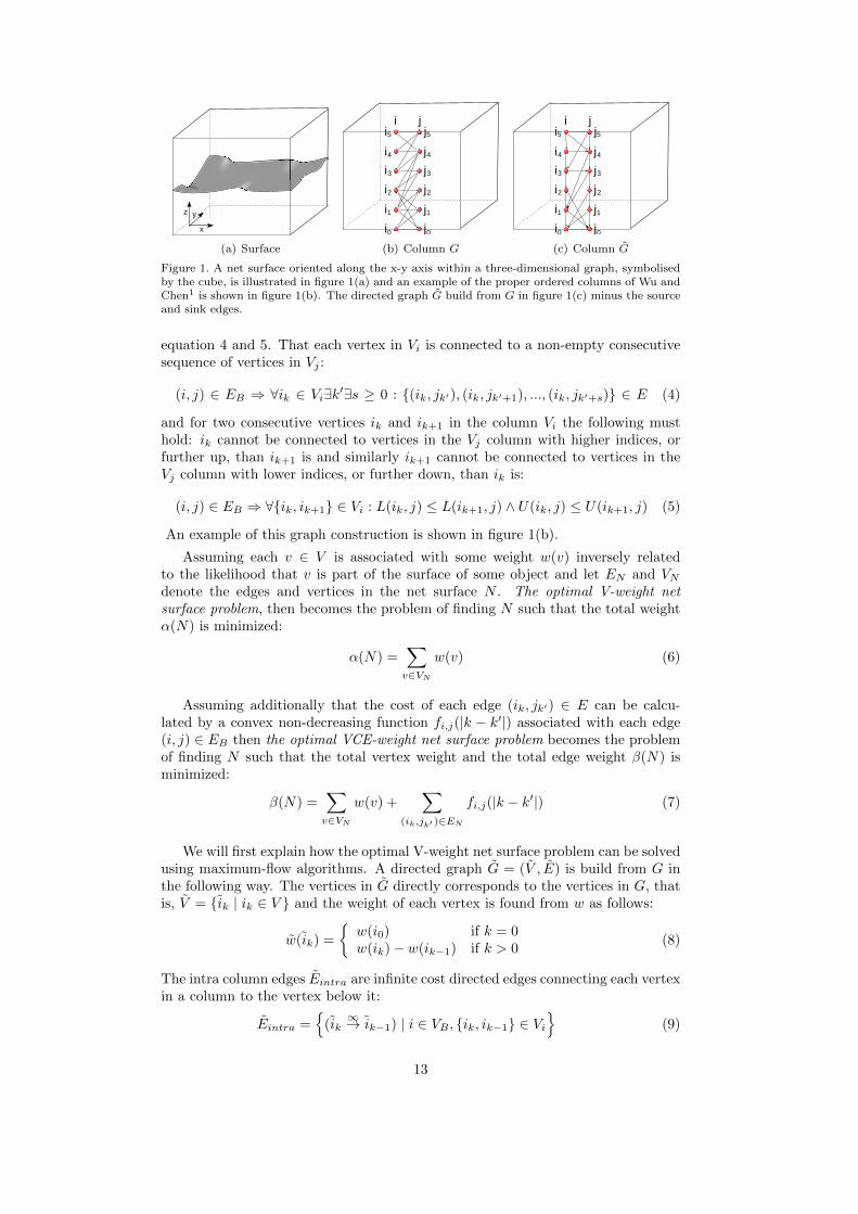
Figure 1. A net surface oriented along the x-y axis within a three-dimensional graph, symbolisedby the cube, is illustrated in figure 1(a) and an example of the proper ordered columns of Wu andChen1 is shown in figure 1(b). The directed graph G build from G in figure 1(c) minus the sourceand sink edges.
equation 4 and 5. That each vertex in Vi is connected to a non-empty consecutivesequence of vertices in Vj :
(i, j) ∈ EB ⇒ ∀ik ∈ Vi∃k′∃s ≥ 0 : {(ik, jk′), (ik, jk′+1), ..., (ik, jk′+s)} ∈ E (4)
and for two consecutive vertices ik and ik+1 in the column Vi the following musthold: ik cannot be connected to vertices in the Vj column with higher indices, orfurther up, than ik+1 is and similarly ik+1 cannot be connected to vertices in theVj column with lower indices, or further down, than ik is:
(i, j) ∈ EB ⇒ ∀{ik, ik+1} ∈ Vi : L(ik, j) ≤ L(ik+1, j) ∧ U(ik, j) ≤ U(ik+1, j) (5)
An example of this graph construction is shown in figure 1(b).
Assuming each v ∈ V is associated with some weight w(v) inversely relatedto the likelihood that v is part of the surface of some object and let EN and VNdenote the edges and vertices in the net surface N . The optimal V-weight netsurface problem, then becomes the problem of finding N such that the total weightα(N) is minimized:
α(N) =∑v∈VN
w(v) (6)
Assuming additionally that the cost of each edge (ik, jk′) ∈ E can be calcu-lated by a convex non-decreasing function fi,j(|k − k′|) associated with each edge(i, j) ∈ EB then the optimal VCE-weight net surface problem becomes the problemof finding N such that the total vertex weight and the total edge weight β(N) isminimized:
β(N) =∑v∈VN
w(v) +∑
(ik,jk′ )∈EN
fi,j(|k − k′|) (7)
We will first explain how the optimal V-weight net surface problem can be solvedusing maximum-flow algorithms. A directed graph G = (V , E) is build from G inthe following way. The vertices in G directly corresponds to the vertices in G, thatis, V = {ik | ik ∈ V } and the weight of each vertex is found from w as follows:
w(ik) =
{w(i0) if k = 0w(ik)− w(ik−1) if k > 0
(8)
The intra column edges Eintra are infinite cost directed edges connecting each vertexin a column to the vertex below it:
Eintra ={
(ik∞→ ik−1) | i ∈ VB , {ik, ik−1} ∈ Vi
}(9)
13

Given a vertex ik in one column and the bottom-most of all the connected verticesin an adjacent column j, jL(ik,j) then the corresponding vertices in G, ik and jL(ik,j)
are connected with a directed edge of infinite cost. We call these the inter columnedges Einter:
Einter ={
(ik∞→ jL(ik,j)) | (i, j) ∈ EB , ik ∈ Vi
}(10)
Next we need to connect the source node s and the sink node t. Let V + and V −
denote the set of vertices in G with non-negative and negative weights respectively:
V + = {v | w(v) ≥ 0} (11)
V − = {v | w(v) < 0} (12)
Then the source and sink node edges, denoted Es and Et respectively, are given by:
Es ={
(s−w(v)→ v) | v ∈ V −
}(13)
Et ={
(vw(v)→ t) | v ∈ V +
}(14)
The intra and inter column edges together with the source and sink node edgesdefine the complete edge set of G, E = Eintra ∪ Einter ∪ Es ∪ Et. An example ofsuch a graph minus the source and sink edges is given in figure 1(c). The minimumcut in G, can be thought of as a segmentation of the object and background vertices,as the vertices in the source and sink sets respectively. The surface N is given bythe top-most vertex in each column that is part of the source set.
Obviously the cut cannot include any edges with infinite capacity, and so thefound surface must be flat, in the sense that if some vertex is in the source set ofthe cut, then every vertex below it, in its column, must also be in the source set. Itcan be argued similarly that it can only follow edges in the graph G.
The solution can be shown to be minimal in α(N) by observing that a net in Gdefines a closed set of all the vertices ”below” it in G. And reversely any non-emptyclosed set in G similarly define a net in G. The net and the corresponding closedset have the same weight, because of the way the weights in G were assigned. Thismeans that finding the minimum closed set in G yields the solution to the optimalV-weight net surface problem. There is one caveat though, the minimum closedset can be empty, which means that every non-empty closed set must have positiveweight. In these cases a simple, so called, translation operation can be performedto change the weight of any bottom vertex, say i0 ∈ V to ensure that a closed sethas negative weight, w(i0) := w(i0) − 1 −
∑j∈VB
j0. This can be done, becausethese vertices are part of any non-empty closed set, and so the operation does notchange any minimal non-empty closed set. Next we need to show that a cut in Gcorrespond to a minimum closed set. Let S and T denote the source and sink setsrespectively in a finite cost cut in G. Notice that the edges in the cut are given by
{(v w(v)→ t) | v ∈ S ∩ V +}∪{(s −w(v)→ v) | v ∈ T ∩ V −}, which leads us to a total costof the cut of
∑u∈S w(u) −
∑v∈V − w(v).
∑v∈V − w(v) is a constant and S is the
source set, defining a closed set. This means the cost of the cut is only a constantfrom the cost of the corresponding closed set and so it must be the minimum closedset.
Next we will describe how the optimal VCE-weight net surface problem can besolved using maximum-flow algorithms. Assuming the directed graph G has beenconstructed as in the optimal V-weight net surface problem. Let I(ik, j) be defined
14
i j
i2
j4f ij(0)
f ij(1)
f ij(2)
f ij(3)
(a) G
i j
i2
j4ij(0)
ij(1)
ij(2)
�
�
�
(b) G
i j
i2
j4Cut
(c) Example Cut
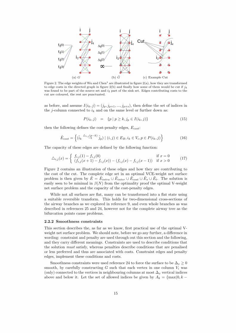
Figure 2. The edge weights of Wu and Chen1 are illustrated in figure 2(a), how they are transformedto edge costs in the directed graph in figure 2(b) and finally how some of them would be cut if j4was found to be part of the source set and i2 part of the sink set. Edges contributing costs to thecut are coloured, the rest are punctuated.
as before, and assume I(ik, j) = (jp, jp+1, ..., jp+s), then define the set of indices inthe j-column connected to ik and on the same level or further down as:
P (ik, j) = {p | p ≥ k, jp ∈ I(ik, j)} (15)
then the following defines the cost-penalty edges, Ecost:
Ecost ={
(ik4i,j(p−k)→ jp) | (i, j) ∈ EB , ik ∈ Vi, p ∈ P (ik, j)
}(16)
The capacity of these edges are defined by the following function:
4i,j(x) =
{fi,j(1)− fi,j(0) if x = 0(fi,j(x+ 1)− fi,j(x))− (fi,j(x)− fi,j(x− 1)) if x > 0
(17)
Figure 2 contains an illustration of these edges and how they are contributing tothe cost of the cut. The complete edge set in an optimal VCE-weight net surfaceproblem is then given by E = Eintra ∪ Einter ∪ Ecost ∪ Es ∪ Et. The solution iseasily seen to be minimal in β(N) from the optimality proof the optimal V-weightnet surface problem and the capacity of the cost-penalty edges.
While not all surfaces are flat, many can be transformed into a flat state usinga suitable reversible transform. This holds for two-dimensional cross-sections ofthe airway branches as we explored in reference 9, and even whole branches as wasdescribed in references 25 and 24, however not for the complete airway tree as thebifurcation points cause problems.
2.2.2 Smoothness constraints
This section describes the, as far as we know, first practical use of the optimal V-weight net surface problem. We should note, before we go any further, a difference inwording: constraint and penalty are used through out this section and the following,and they carry different meanings. Constraints are used to describe conditions thatthe solution must satisfy, whereas penalties describe conditions that are penalisedor less preferred and thus are associated with costs. Constraint edges and penaltyedges, implement these conditions and costs.
Smoothness constraints were used reference 24 to force the surface to be ∆x ≥ 0smooth, by carefully constructing G such that each vertex in one column Vi was(only) connected to the vertices in neighbouring columns at most ∆x vertical indicesabove and below it. Let the set of allowed indices be given by Ak = {max(0, k −
15

x
i j
(a) Column G
x
i j
(b) Column G
Figure 3. Column in a graph enforcing the smoothness constraints introduced in reference 24, seenin figure 3(b). Feasible surfaces can at most change ∆x = 3 vertical levels between two columns.The directed graph constructed from G minus the source and sink edges shown in figure 3(b).
∆x),max(0, k−∆x) + 1, ...,min(K − 1,∆x + k)}, then these smoothness constraintedges, Einter, are given by:
Einter ={
(ik, jk′) | (i, j) ∈ EB , ik ∈ Vi, k′ ∈ Ak}
(18)
Example seen in figure 3. This forces any feasible surface to at most change ∆x
vertical indices between two connected columns:
(ik, jk′) ∈ EN ⇒ |k − k′| ≤ ∆x (19)
The method was used to segment the cylindrical surfaces of human airway segmentsfrom pulmonary volumetric CT images by ’unfolding’ them into flat surfaces. Withthe surfaces oriented along the (x−y)-axis, see figure 1(a), x and y axis smoothnessconstraints, ∆x ≥ 0 and ∆y ≥ 0 were used to guarantee surface continuity inthree dimensions. An expert compared the segmentation results in 100 randomlyextracted perpendicular cross-sectional images from 317 airway segments with astrictly two-dimensional method and found the vast majority to be superior.
2.2.3 Coupled surfaces
Li et al.25 were the first to show how multiple flat surfaces could be coupled intoone maximum flow graph, by combining the intra surface edges of Wu and Chen,1
with inter surface edges to constrain the surface separation. This coupled surfacegraph cut algorithm could combine the information of the image at the regionof the multiple surfaces and thereby use clues from one surface to help place theother. This is extremely useful for airway wall segmentation, as the two borders areinherently connected.
n proper ordered multi-column graphs Gm, m ∈ {0, 1, ..., n − 1} are needed tosegment n surfaces using this method, all the same size, but they can be associatedwith different vertex and edge weights. These graphs are then combined:
G ={Gm = (V m, Em) | m ∈ {0, 1, ...n− 1}
}∪{Emsep | m ∈ {0, 1, ..., n− 2
}(20)
Assuming Gm and Gm+1 are the graphs of two surfaces, whose separation needsto be constrained, let V mi ∈ V m and V m+1
i ∈ V m+1 denote corresponding columnsin each of these graphs respectively, let imk ∈ V mi and im+1
k′ ∈ V m+1i be vertices in
each of the columns and let δm,m+1l and δm,m+1
u define a lower and an upper boundrespectively on the signed surface separation:
(imk , im+1k′ ) ∈ EN ⇒ δm,m+1
u ≥ k − k′ ≥ δm,m+1l (21)
16

i
�
m, m+1
m, m+1
�
mim+1
l
u
(a) Column G
i
�
m, m+1
m, m+1
�
mim+1
l
u
(b) Column G
Figure 4. Figure 4(a) shows an example column implementing the separation constraints of refer-
ence 25 with δm,m+1l = 1 and δm,m+1
u = 3. Figure 4(b) illustrates the directed graph constructedfrom G minus the source and sink edges. The blue vertices are deficient nodes.
We will assume without loss of generality that δm,m+1u ≥ 0, because if this is not the
case, then either the constraints represent an infeasible solution or we may simplyswitch the indices of Gm and Gm+1. Let Tm = {δlm,m+1, δ
lm,m+1 + 1, ..., δum,m+1},
and define the set of allowed indices as Am,m+1k = {max(0, k− δm,m+1
u ),max(0, k−δm,m+1u )+1, ...,min(K−1, k−δm,m+1
l )} then the surface separation constraints areimplemented by the Esep edges:
Esep ={
(imk , im+1k′ ) | m ∈ {0, 1, ..., n− 2}, t ∈ Tm, imk ∈ V mi , k′ ∈ Am,m+1
m
}(22)
The directed graph is then constructed from G as described in section 2.2.1. Notethat some vertices in the top and bottom of these columns are not strongly connectedand they cannot appear in any feasible solution. Reference 25 calls such verticesdeficient nodes. In order to make the graph a proper ordered multi-column graph,such vertices and their incident edges need to be removed. Figure 4 illustrates thisgraph construction method.
The original paper25 verified the method on phantoms and 3D medical imagesfrom CT, magnetic resonance (MR) and ultrasound scanners. Amongst these testwere segmentations of the inner and outer airway wall surfaces in 12 in vivo CTscans of 6 humans subjects. The segmentations were conducted on unfolded airwaysegments. The results were found to be statistically more accurate when comparedwith previous two-dimensional methods.
The method has later been used for various segmentation problems, such as thesegmentation of six63 and seven64 intraretinal layer surfaces in 24 three-dimensionalmacular optical coherence tomography images from 12 subjects also with promisingresults.
2.2.4 Edge penalties
Even though the optimal V-weight net surface problem has found multiple usessince it was first described, only one paper (to our knowledge) contain a practicaldescription of the usage of the optimal VCE-weight net surface problem. It occurredin reference 56, where it was used in combination with smoothness and separationconstraints to segment liver lesions with necrosis or calcification and various othertumors in CT images. The implemented smoothness and separation penalties makeit possible to penalise surfaces further from being smooth and close together. Wewill not describe the graph construction method, as it is the logical extension of thespecific optimal V-weight net surface problems, already described in section 2.2.2and section 2.2.3, to the optimal VCE-weight net surface problem, described insection 2.2.1, instead we included an illustration of the technique in figure 5. The
17

x
i j
(1)
m m
m
(2)
(0)
(3)
fi ,jm
fi ,jm
fi ,jm
fi ,jm
(a) Smoothness
i
(1)
(2)
(3)
im m+1
gi m
�
m, m+1
m, m+1
�l
ugi
m
gi m
(b) Separation
Figure 5. The edge penalties of reference 56 here shown as non-directed graphs with ∆mx = 3,
δm,m+1l = 1 and δm,m+1
u = 3. Figure 5(a) shows an example of the smoothness penalty with edgecosts given by the function: fmi,j(x) and figure 5(b) shows an example of the separation penalty
with edge costs given by the function: gmi (x). Deficient nodes are shown in blue.
practical experiment conducted made use of smoothness penalties only and notseparation penalties. The edge cost function was chosen as:
fmi,j(x) = x2,m ∈ {0, 1}, (i, j) ∈ EB (23)
The results on the synthetic data show that the smoothness penalty enables themethod to better cope with noise in the data, and according to the authors themethod’s capability to simultaneously identify liver tumor and necrosis boundariesis unprecedented.
2.2.5 Segmentation of non-flat surfaces
Li et al.3 expanded the coupled surface methods to be able to handle multiple closedsurfaces by constructing each column at surface points and orienting it in the samedirection as the surface normal. The method was demonstrated by segmentinga three-dimensional magnetic resonance image of an human ankle and validatedagainst manual segmentations.
The method has later been used to segment the liver in 54 CT images, using astatistical shape model along with an evolutionary algorithm to detect the initialsegmentation.5 In reference 6 a multi-object extension of the method was used tosegment the knee-joint bone and cartilage in 17 three-dimensional MR data sets. Inreference 7 the method was used to segment the femoral head, ilium, distal femurand proximal tibia in CT data.
The method is vulnerable to self-intersections due to its reliance on surfacenormals.
2.2.6 Medial axes columns
Liu et al.4 used the medial axes to find the normal direction and column lengths.The medial axis of the initial segmentation is a set of points, each of which has atleast two nearest points on the surface. The distance from a surface point to thenearest medial axis point is a conservative bound on the distance one can travelalong the normal direction, while keeping the surface point the nearest surfacepoint. This is also known as the local feature size or local thickness. By using thisdistance as column length, the columns can be guaranteed not to be intersecting.The medial axis is complicated to compute, but approximations can be found usingDelaunay/Voronoi diagrams of the surface points.65
18
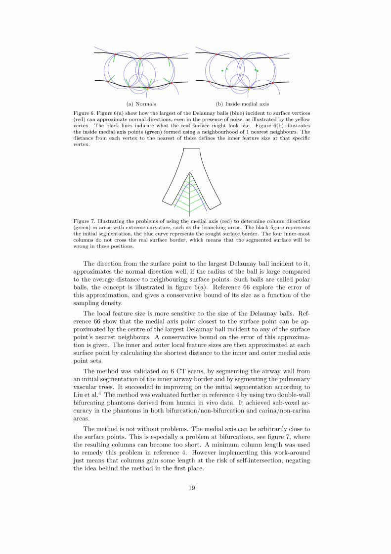
(a) Normals (b) Inside medial axis
Figure 6. Figure 6(a) show how the largest of the Delaunay balls (blue) incident to surface vertices(red) can approximate normal directions, even in the presence of noise, as illustrated by the yellowvertex. The black lines indicate what the real surface might look like. Figure 6(b) illustratesthe inside medial axis points (green) formed using a neighbourhood of 1 nearest neighbours. Thedistance from each vertex to the nearest of these defines the inner feature size at that specificvertex.
Figure 7. Illustrating the problems of using the medial axis (red) to determine column directions(green) in areas with extreme curvature, such as the branching areas. The black figure representsthe initial segmentation, the blue curve represents the sought surface border. The four inner-mostcolumns do not cross the real surface border, which means that the segmented surface will bewrong in these positions.
The direction from the surface point to the largest Delaunay ball incident to it,approximates the normal direction well, if the radius of the ball is large comparedto the average distance to neighbouring surface points. Such balls are called polarballs, the concept is illustrated in figure 6(a). Reference 66 explore the error ofthis approximation, and gives a conservative bound of its size as a function of thesampling density.
The local feature size is more sensitive to the size of the Delaunay balls. Ref-erence 66 show that the medial axis point closest to the surface point can be ap-proximated by the centre of the largest Delaunay ball incident to any of the surfacepoint’s nearest neighbours. A conservative bound on the error of this approxima-tion is given. The inner and outer local feature sizes are then approximated at eachsurface point by calculating the shortest distance to the inner and outer medial axispoint sets.
The method was validated on 6 CT scans, by segmenting the airway wall froman initial segmentation of the inner airway border and by segmenting the pulmonaryvascular trees. It succeeded in improving on the initial segmentation according toLiu et al.4 The method was evaluated further in reference 4 by using two double-wallbifurcating phantoms derived from human in vivo data. It achieved sub-voxel ac-curacy in the phantoms in both bifurcation/non-bifurcation and carina/non-carinaareas.
The method is not without problems. The medial axis can be arbitrarily close tothe surface points. This is especially a problem at bifurcations, see figure 7, wherethe resulting columns can become too short. A minimum column length was usedto remedy this problem in reference 4. However implementing this work-aroundjust means that columns gain some length at the risk of self-intersection, negatingthe idea behind the method in the first place.
19

(a) Electric lines of force (b) Columns
Figure 8. Figure 8(a) show two-dimensional simulated electric lines of force from 7 point charges.Figure 8(b) illustrates the idea behind the use of the non-intersection property of the electric linesof force (green), when used to construct columns. Notice that they all cross the sought surface(blue) and none intersect.
2.2.7 Electric lines of force inspired columns
Recently a paper was published on a novel graph construction technique, which wasinspired by the non-intersection property of the electric lines of force.2 Instead ofusing straight columns, the columns follow the electric field direction. RememberCoulomb’s law, says that the magnitude, Ei, of the electric field created by a singlepoint charge, qi, at a certain distance, ri, is:
Ei =1
4πε0
qir2i
,
where ε0 is the electric constant. For a system of discrete charges, Ei, where i ∈{1, 2, ..., n}, the magnitude E is given by the sum of the individual charges:
E =
n∑i=1
Ei
The electric lines of force follow the direction of the electric field, the directionwithin the field, which has the greatest rate of change, see figure 8(a).
Reference 2 assign unit charges to the surface points of the initial model andtrace the columns using an electric field with magnitude E′i = 1/r4
i . This was doneto reduce the effect of distant charges and does not compromise the non-intersectionproperty. Figure 8(b) illustrates how the non-intersection property might help forinstance in bifurcation areas.
The method was demonstrated using iterative graph searching of a tibial bone-cartilage interface and in a multi-surface graph search segmentation of mutuallyinteracting femoral and tibial cartilage with promising results. The authors com-mented that the method’s most significant limitation is the relative expensive com-putation of the electric lines of force.
2.2.8 Cost functions
An integral part of most optimisation problems, is the ability to assign a cost toany given solution. A cost function fills this role by mapping some set of inputvariables to a cost. Within the subject at hand, this cost should reflect the inverselikelihood that any given input point belongs to the airway wall border. Specificallywe need one cost function to so pinpoint the inner airway wall border and anotherto so specify the outer airway wall border.
Note that some of the specific methods explained in this section, are actuallyreward functions, in the sense that their returned values are highest at likely edgepositions.
20

R∂R∂t
∂2R∂2t
Ci
Co
Inner edge Outer edge
Figure 9. Ray intensity values R, ray derivatives ∂R/∂t and ∂2R/∂2t and the inner and outercost functions Ci and Co from reference 9. Notice that the extrema of the first and second orderderivatives occur at different sides of the edges.
The matter of constructing such a cost function is inherently an edge detec-tion problem, and many of the methods already described, such as FWHM, phasecongruency21 or the approaches using models and parameters to approximate scan-ner specifics19,50 could be used with modifications. Classic edge detectors such asCanny67 or Deriche68 are also good options.
Many methods take the approach of using derivative filters to highlight the edges.For instance reference 3 used the negated gradient magnitude, −|∆I|, of a Gaussiansmoothed image as a bone specific cost function and weighted combinations of theeigenvalues of the Hessian matrix of the image intensity as a cartilage specific costfunction. Reference 56 used −|∆I| to detect the tumor layer and the first derivativein the column direction to detect the necrosis layer.
Reference6 defined the cost function based on the magnitude of the image gra-dient as e−|∆I|/2 and modified the values by adding or subtracting constants de-pending on whether the intensity values were increasing or falling and whether thesearch was toward cartilage or away from cartilage.
Reference7 derived a cost function based on simple thresholding of the imageintensities. Costs were simply defined to be low where intensities changed fromabove to below the threshold.
A common approach is to use the fact that the first and second order derivativeedge detectors place their maximums on different sides of the sought edge. Weight-ings of these can therefore be used to adjust the position of the found edge, in orderto match some form of ground truth data.4,9, 20,22,24,25 For instance reference 4,22and 24 used weightings of the Marr-Hildreth and Sobel masks. Reference 20 in-troduced boundary specific cost functions based on this concept, designed to findeither the inner or the outer airway wall border. However the second order deriva-tive used, added positive responses at both borders, leading to situations wherethe borders could be found on top of each other. We therefore modified the costfunctions slightly in reference 9 to remove the second order derivative componentat the wrong border. These inner and outer cost functions, Ci and Co respectively,are given by equations 26 and 27. But first denote the positive and negative partsof the first order derivative in the column direction by P (t) and N(t):
P (t) =∂R
∂t
(t)H(∂R∂t
(t))
(24)
N(t) =∂R
∂t
(t)(
1−H(∂R∂t
(t)))
, (25)
21

where R(t) is the intensity of a ray going from the lumen through the wall and intothe parenchyma, parameterised by t. H is some continuous approximation of theHeaviside step function. Then the inner and outer cost functions were defined byCi and Co using weights γi ∈ [0, 1] and γo ∈ [0, 1] in the following manner:
Ci(t) = γiP (t) + (1− γi)∂P
∂t
(t)
(26)
Co(t) = (1− γo)∂N
∂t
(t)− γoN(t) (27)
Figure 9 illustrates the concept.
A cost function based on a combination of first and second order derivativeweightings, edge orientation preference and a position penalty term was suggestedin reference 25. The orientation and position penalties may incorporate a prioriknowledge about the rotation and position of the edge. A cost function tailored tooptimal net type columns and based on the piecewise constant minimal variancecriterion of Chan and Vese,69 was also proposed:
C(ik) =
k∑j=0
(I(ij)− a1
)2+
K−1∑j=k+1
(I(ij)− a2
)2, i ∈ EB , ik ∈ Vi, (28)
where I is the image intensity function. a1 and a2 should ideally be the meanintensity inside and outside the object respectively, but since the object is unknownbefore segmentation, approximations must be used:
a1(ik) = mean({ik′ | 0 ≤ k′ ≤ k}
)and (29)
a2(ik) = mean({ik′ | k < k′ < K}
), i ∈ VB , ik ∈ Vi (30)
This cost function definition attempts to minimize the image intensity varianceinside and outside the object.
The many coupled surfaces of reference 63, 64 required a lot of different costfunction definitions. Combinations of Sobel masks and pixel intensity summation inlimited regions were implemented to favour dark-to-light or light-to-dark transitionswith dark or light regions above or below the surfaces. A cumulative summationof pixel intensities along the columns were used to discourage finding bright pixelsabove or below the surface. The Chan and Vese minimal variance term, explainedabove, was also used for a single surface.
2.3 Airway abnormality measures
This section contains a description of previous airway abnormality measures usedto quantify COPD development. We are not aware of any three-dimensional airwayabnormality measures, probably due to the fact that practically all previously pub-lished studies investigating COPD have been using one- or two-dimensional auto-matic, semi-manual or manual segmentation methods.9,45,45,47,48,51,52,54,55,70,70–74
The following metrics thus all require the existence of some segmented two-dimen-sional airway cross-section ideally oriented perpendicular to the airway centreline.
The most commonly reported metrics are the Inner Area (IA) also called thelumen area and the Wall Area percentage (WA%). WA% is the percentage of theairway area that is wall: WA% = 100×WA/(IA+WA)%. Both measures have beenconsistently correlated with lung function measurements in the past.46–48,51,71–73
Generally smaller measures of IA and larger measures of WA% are associated witha worse lung function. IA is a problematic measure, given that it contains nonormalisation. This means it is likely more sensitive to covariates such as weight,
22

height and sampling positions. A problem with WA% is that the changes to themeasure caused by COPD are relatively small. For instance the difference betweenthe sickest and healthiest are on the order of a few percentage points.9,46 Thiscombined with the fact that the analysed airways are close in size to the resolutionof the images, means that segmentation errors or even discretisation effects veryquickly obscure any change caused by COPD.
Intensity or density based measures introduced recently9,47 should be more ro-bust to such errors. This is because they may be more sensitive to the size of imagedstructures, when such structures are small compared to the imaging resolution, dueto partial volume effects. It has also been theorised that the average density of theairways increase with disease progression, due to mural calcification and fibrosis,47
which would further increase their usefulness. Peak Wall Attenuation (PWAt)47
and Normalised Wall Intensity Sum (NWIS)9 are measures introduced to try tocapture such effects. PWAt is defined as the mean of the maximum intensity foundwithin the wall along rays cast 360 degrees around the centre and out. NWIS is anormalised measure of mass changes within the airway wall and is defined as thesum of the intensities plus 1000 within the wall area normalised by the total air-way area: NWIS =
∑x∈WA(I(x) + 1000)/(WA+IA), where WA denotes the set of
points inside the wall. PWAt and NWIS have been found previously9,47 to corre-late equally or more with lung function, to be more reproducible and have betterdiagnostic ability than size based measures such as IA and WA%. Higher values ofPWAt and NWIS were found to be associated with poorer lung function.
The broncho-arterial ratio is based on the fact that most airways are accompa-nied by an artery. These two structures have similar diameters in healthy individu-als, but in COPD subjects, the lumen narrows. It is therefore possible to normalisethe lumen diameter by dividing with the arterial diameter.54,55,74 Increasing val-ues of the ratio have been shown to be associated with lower lung function.74 Aproblem with the measure, is that it can be very difficult to automatically identifythe accompanying artery.
Having a single number for each CT scan is attractive for diagnostic purposesand it can be achieved by simply averaging all the measurements sampled in somebranch generation range.9,51 However this introduces errors due to differences in thebranches found by the segmentation. PI10 is a measure which was designed to beconsistent in the face of such differences. The measure is based on the assumptionthat there is a linear relationship between the square root of WA and the internalperimeter (PI) of the airway.45,70 Using linear regression of the sampled values ofWA and PI it is thus possible to calculate what WA would be, if it was sampled atany specific position in the airway. PI10 is the WA so sampled at a PI of 10 mm.We investigated the measure in reference 9 and found the results disappointing. Itproved to be the least reproducible of all the examined measures, likely because theuse of linear regression makes the measure very sensitive to outliers.
Note that this list is by no means complete, the size changes have been quantifiedin many more ways. However it does represent some of the most common metrics.
3. METHOD
In this section our approach to airway wall segmentation and measurements will bedescribed. Starting with a short description of the employed airway segmentationmethod and how additional information, such as the position of the airway centre-lines, the position of the bifurcation regions and the branch generation numbers weregenerated. Then we will describe specifics of the investigated graph constructionmethods, including our novel column construction technique with columns following
23

flow lines. We will describe the used cost functions, the training and evaluation ofthe methods and the statistical investigations performed.
3.1 Airway segmentation
No specific algorithm can be said to be the best airway segmentation algorithm atthe moment. Judging by the Exact’09 study some, such as reference 30 and 38stand out as being very exploratory and get larger tree lengths and branch counts.Whereas other such as reference 34 are very conservative and thus get very fewfalse-positives, but also very short tree lengths and low branch counts.
The airway wall segmentation will assume some degree of correctness in theinitial segmentation, provided by the airway segmentation method, in the sensethat only minor offsets are needed to find the correct segmentation. This meansthat if leaks occur, which usually completely change the segmentation, the resultingairway wall segmentation will likely also be wrong.
If the goal of the combined algorithm is to diagnose a disease such as COPD,whose effects are widespread within the airways but very small in relative size, thena small false positive rate is probably more important than a small false negativerate. For instance, as described, the very commonly reported airway abnormalitymeasure, WA%, only varies a few percent between sick and healthy, but a single leakmight change the complete airway volume by many percentage points, completelyinvalidating the measurement.
Another important point is consistency. Airway abnormality measures are un-fortunately not independent from the physical position in the airway in which theyare measured and no good method exist, which can compensate or normalise forthis dependency. So airways should ideally be resolved to a roughly similar depthand including roughly the same branches in each segmentation, in order to getreproducible measurements.
We used the method of reference 33 to segment the airways. It has a verylow false-positive rate, just slightly worse than the most conservative method34
participating in the Exact’09 study.28 Yet the branch detection rate and the treelength are not far from the most exploratory methods.
The method incorporates trained local airway appearance models and uses thefact that an airway is always accompanied by an artery. The orientation of bothstructures are used as a criterion for region growing. This works well becausearteries are easier to detect than airways.
3.2 Tree extraction
There is general agreement12 that COPD mostly affects the smaller airways, sowe need some way of splitting the airways into regions based on their local size.We want this split to be independent of disease progression, in order to not biasthe results, so it cannot for instance be based on just the size of the measuredstructures, as these are known to be affected. An anatomical consistent way to doit, is to simply do it based on the generations of the airway branches.
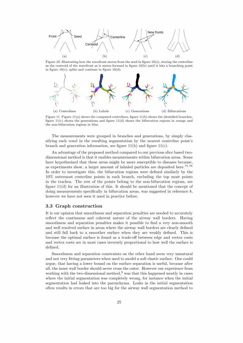
We therefore extracted the centrelines, branches and generation numbers fromthe airway tree with a front propagation method, as described in reference 28.Using the initial segmentation and starting in the trachea, the centroid of the frontis stored as the branch centreline as it moves down into the bronchi. Bifurcationsare detected as the wavefront becomes disconnected upon hitting bifurcation points,see figure 10.
The computed centrelines were also to used to extract cross-sections used tobuild the training and test set mentioned in section 3.5.
24
SeedFront
(a)
Centroid
Centerline
(b)
New fronts
(c) (d)
Figure 10. Illustrating how the wavefront moves from the seed in figure 10(a), storing the centrelineas the centroid of the wavefront as it moves forward in figure 10(b) until it hits a branching pointin figure 10(c), splits and continue in figure 10(d).
(a) Centrelines (b) Labels (c) Generations (d) Bifurcations
Figure 11. Figure 11(a) shows the computed centrelines, figure 11(b) shows the identified branches,figure 11(c) shows the generations and figure 11(d) shows the bifurcation regions in orange andthe non-bifurcation regions in blue.
The measurements were grouped in branches and generations, by simply clas-sifying each voxel in the resulting segmentation by the nearest centreline point’sbranch and generation information, see figure 11(b) and figure 11(c).
An advantage of the proposed method compared to our previous slice based two-dimensional method is that it enables measurements within bifurcation areas. Somehave hypothesized that these areas might be more susceptible to diseases because,as experiments show, a larger amount of inhaled particles are deposited here.75,76
In order to investigate this, the bifurcation regions were defined similarly by the10% outermost centreline points in each branch, excluding the top most pointsin the trachea. The rest of the points belong to the non-bifurcation regions, seefigure 11(d) for an illustration of this. It should be mentioned that the concept ofdoing measurements specifically in bifurcation areas, was suggested in reference 8,however we have not seen it used in practice before.
3.3 Graph construction
It is our opinion that smoothness and separation penalties are needed to accuratelyreflect the continuous and coherent nature of the airway wall borders. Havingsmoothness and separation penalties makes it possible to find a very non-smoothand well resolved surface in areas where the airway wall borders are clearly definedand still fall back to a smoother surface when they are weakly defined. This isbecause the optimal surface is found as a trade-off between edge and vertex costsand vertex costs are in most cases inversely proportional to how well the surface isdefined.
Smoothness and separation constraints on the other hand seem very unnaturaland not very fitting parameters when used to model a soft elastic surface. One couldargue, that having a lower bound on the surface separation is useful, because afterall, the inner wall border should never cross the outer. However our experience fromworking with the two-dimensional method,9 was that this happened mostly in caseswhere the initial segmentation was completely wrong, for instance when the initialsegmentation had leaked into the parenchyma. Leaks in the initial segmentationoften results in errors that are too big for the airway wall segmentation method to
25
correct, the best one can do therefore is to detect them, and not include them inthe measurements. Not having a lower bound on the surface separation enables usto discard a lot of these areas as the places where the inner surface overlaps theouter. Section 3.6 contains a description of how it was used in practice.
Unfortunately the performance of the described optimal net based surface sepa-ration penalty is related to δ0,1
u and δ0,1l in such a way that performance gets worse
if the surface is constrained less and the performance of the smoothness penaltiesare similarly related to the smoothness constraints ∆0
x and ∆1x. To see why notice
that the amount of edges added in two corresponding columns as a consequence ofthe separation penalty and the separation constraint is given by:
K−1∑k=0
(min(K − 1, k − δ0,1
l )−max(0, k − δ0,1u ) + 1
)(31)
As an example, assume that K = 10, δ0,1u = 3 and δ0,1
l = 1, which results in 24 edges,the same case with δ0,1
u = 6 results in 39 edges, and the completely unconstrainedcase results 100 edges. The amount of edges added in two neighbouring columnsdue to the smoothness penalty and the smoothness constraint is given by:
K−1∑k=0
(min(K − 1, k + ∆m
x )−max(0, k −∆mx ) + 1
),m ∈ {0, 1} (32)
This adds up to 3×K2 edges with two surfaces, no constraints and only penalties.So the conclusion is that constraints are probably needed, if for nothing else thanperformance reasons. If the edge cost function fi,j(|k − k′|) is linear and doesnot depend on the indices i and j, then our graph construction technique fromreference 9, which we will describe and extend to three dimensions in the following,offers a much simpler solution. It has at most 3∗(Kmean−2) edges as a consequenceof its smoothness and separation penalties, where Kmean is the average number ofvertices in each column. It also only has |VB | ∗ 2 source and sink edges comparedto the |VB | ∗K used in the optimal net type of graph. Both graphs have a similaramount of intra-column edges. It should be noted that many of the optimal netedges do not have to be stored explicitly, because they have infinite cost, howeverin loosely constrained graphs the non-infinite cost edges will still dominate.
We will specify the graph construction for a single surface, denoted m first. Thiswill then be expanded to multiple surfaces, using a coupled surface graph later.We will use the same technique of specifying the problem in terms of a base graphGmB = (V mB , EmB ), which can be mapped into an undirected graph, Gm = (V m, Em),with vertices, V m, and edges Em, by associating each vertex i in the base graph witha column of vertices in V m, denoted V mi . Lets assume that each i is associated withIi and Oi points inside and outside the initial segmentation respectively. Combinedwith the initial surface point, i0, these points represents the column V mi :
V mi = {i−Ii , i1−Ii , ..., i0, ..., iOi}, for i ∈ V mB . (33)
Just as in the Optimal Net type of methods, a column represent the space of all pos-sible solutions, a sought surface point can take. But unlike the Optimal Net type ofcolumns, we will not require that they have equal length. We will deal with differentways of constructing columns in section 3.3.2 and 3.3.3. The columns are connectedin a neighbourhood, reflecting the topology of the surface, see section 3.3.1. Thevertices, V m, in Gm are given by:
V m = {V mi | i ∈ V mB } (34)
26

w(j )
w(j )w(j )
w(j )
w(i )w(i )
w(i )
w(i )
t
s
1
2
1
-1
2
0
-1
-2
w(j )
0
34
w(i )
w(j )~
~
~
~~
~~
~~
~
~
(a) Intra column edges
p
t
s
p
p
pp
p
(b) Inter column edges
p
t
s
pp
pp
p
Cut
Cut
(c) Example cut
Figure 12. Figure illustrating two connected columns, with edges in black, vertices in red andsource s and sink node t and the initial segmentation surface represented by the grey line. Thecolumns illustrated have inside lengths of Ii = 2 and Ij = 1 and outside lengths of Oi = 3and Oj = 5. Figure 12(a) shows the intra column directed edges with capacities given by atranslated cost function w. Figure 12(b) illustrates the graph when the inter column edges areadded, implementing the smoothness penalty p. Figure 12(c) illustrates how a cut might separatethe source and sink nodes. Edges contributing to the cost of the cut are punctuated.
The undirected graph edges, reflecting every possible solution, are given by:
Em = {(ik, jk′) | (i, j) ∈ EmB , ik ∈ V mi , jk′ ∈ V mj } (35)
The vertices in the graph are associated with weights given by a cost functionwm whose values reflect the inverse likelihood that the sought surface exist at anygiven position, see section 3.4, and the edges have costs implementing a smoothnesspenalty, given by the parameter pm ≥ 0, note that this corresponds to the optimalnet edge cost function fmi,j(|k − k′|) = pm|k − k′|. Later we will explain how thisconstruction is expanded to the dual surface problem at hand.
Gm is transformed into the directed maximum flow graph by adding Ii +Oi + 1vertices associated with each column V mi as follows:
V m ={ik | i ∈ V mB , ik ∈ V mi
}(36)
Directed edges with infinite capacity are then added from the source s to the inner-most vertices, and from the outer-most vertices to the sink t, lets denote them Emsand Emt respectively, as follows:
Ems ={
(s∞→ i−Ii) | i ∈ V mB
}(37)
Emt ={
(iOi
∞→ t) | i ∈ V mB}
(38)
The intra column edges Eintra, associated with the cost function, are given by:
Emintra ={
(ikwm(ik)→ ik+1) | i ∈ V mB , {ik, ik+1} ∈ V mi
}(39)
Notice that the intra edge costs in the directed graph are equal to the correspondingvertex cost in the undirected graph plus a constant, see equation 50. This is illus-trated in figure 12(a). Next we will show how the inter-column edges, implement-ing the smoothness penalty, are added. First we define O(i, j) = max(Oi, Oj) − 1,I(i, j) = max(Ii, Ij) − 1, for any neighbouring column j and the bounded vertexindex B(i, k):
B(i, k) =
−Ii if k < −IiOi if k > Oik else
(40)
27
t
s
(a) Corresponding columns
t
s
q
q
q
q
(b) Inter surface edges
t
Cut
Cut
s
(c) Example cut
Figure 13. The figures show two corresponding columns. The column marked with green arrowsrepresents the inner column and the blue arrowed column represents the outer column. Fig-ure 13(a) shows the graph before the separation penalty edges are added, the inner and outersurface positions are marked with a green and blue line respectively. Figure 13(b) shows the graphafter. The black bidirectional edges are the separation penalty edges. Edges contribution to thetotal cost of the solution are marked with arrows and punctuated lines in figure 13(c), assumingthe solution (cut) is found at the illustrated surface positions.
The inter-column edges Eminter are then given by:
Eminter ={
(iB(i,k)pm↔ jB(j,k)) |(i, j) ∈ EmB ,
k ∈{− I(i, j), 1− I(i, j), ..., O(i, j)
}} (41)
Figure 12(b) contains an illustration of these edges. Notice that the weight of anycut in the graph is a sum of the cut intra and inter column edges. Increasing thevalue of pm will make the intra column edges relatively cheaper to cut, and willthus favor straighter and smoother surfaces.
Next we will explain how the graphs of the surfaces are coupled, implementingseparation penalties qm ≥ 0, associated with the separation between surface mand m + 1. Note that these correspond to the optimal net edge cost functionsgmi (|k − k′|) = qm|k − k′|. The graphs are similar in that they are generated fromthe identical base graphs GmB and their columns have the same length. We thencombine the graphs as previously described:
G ={Gm | m ∈ {0, 1, ..., n− 1}
}∪{Emsep | m ∈ {0, 1, ..., n− 2}
}(42)
where n is the number of surfaces, n = 2 in the application within this thesis.As before let Ii and Oi denote the inside and outside column lengths. Then theseparation penalty edges Emsep, reflecting every possible surface separation, are givenby:
Emsep ={
(imk , im+1k′ ) | im ∈ V mB , im+1 ∈ V m+1
B , imk ∈ V mi , im+1k′ ∈ V m+1
i }}
(43)
The separation edges in the directed graph Emsep are given by:
Emsep ={
(ikqm↔ jk) | i ∈ V mB , j ∈ V m+1
B , k ∈ {−Ii, 1− Ii, ..., Oi}}
(44)
Figure 13 show the inner and outer columns before and after the inter surface edgesare added. Notice that increasing the value of qm, will make cuts that are separatedin the inner and outer columns, progressively more expensive, and will thus causethe method to favour closer surfaces.
28

The complete directed graph G is given by:
V ={
˜V m | m ∈ {0, 1, ..., n− 1}}
(45)
E ={Ems ∪ Emt ∪ Emintra ∪ Eminter | m ∈ {0, 1, ..., n− 1}
}∪{
Emsep | m ∈ {0, 1, ..., n− 2}} (46)
G = (V , E) (47)
Maximum flow algorithms always find the global optimal solution, so the solutionis naturally going to be optimal in the sum of the cost of the cut intra, inter andseparation penalty edges. However we want to prove that it is also an optimalsolution to the instances of the optimal VCE-weight net surface problem defined byequation 42. Lets first redefine N to include variable length columns:
N : {Vi | i ∈ VB} → {i−Ii , i1−Ii , ..., iOi} (48)
Note that the original problem set is a subset of this, and so it does not affect theproof.
Notice that every column in G must be cut, since they define a direct line offlow from the source to the sink. In some degenerate cases columns might be cutmultiple times, that is the cut surface contains folds (or loops). This can be avoided,by observing, that such a cut would always include more intra column edges than anon-folded cut. It is easy to see that increasing the cost of every intra column edgewith a constant, does not affect the choice of non-folded minimum cut, howeverpossible minimum cuts with folds gets progressively more expensive. So all we needto know is how much to increase the cost of each intra column edge to avoid foldsin the solution. The reason a minimum cut might contain folds in the first place,is because it could potentially decrease the total cost of the cut inter column andseparation edges. A simple bound on this cost is given by:
ϕ =
n−2∑m=0
|Emsep| ∗ qm +
n−1∑m=0
|Einter| ∗ pm (49)
Note that smaller numbers will do. This can be used to perform an operation,similar to the translation operation described in section 2.2.1:
wm(v) = wm(v) + ϕ, for v ∈ V m (50)
Now because of the way the graph is constructed, if a vertex is part of the sink set,in a minimum cut, then every vertex following it must be as well:
ik ∈ T ⇒ ik+1 ∈ T, for m ∈ {0, 1, ..., n− 1}, i ∈ EmB , {ik, ik+1} ∈ V mi , (51)
The conclusion is, that a minimum cut in G is a net surface in G. It can alsobe seen that any possible net surface in G also defines a cut in G, since it canbe thought of as partitioning of the vertices into two disjoint subsets, with thesource in one set and the sink in the other. The cost of such a cut in G is givenby the sum of the costs of the cut intra and inter column and separation edges.The cost of the cut intra column edges is easily seen to be equal to the vertexcost in the corresponding net surface
∑v∈VN
w(v), plus a constant. To explainwhy the inter column edge construction corresponds to an edge cost function offmi,j(|k − k′| = pm|k − k′|, lets assume without loss of generality that k ≤ k′, andnotice that if ik ∈ V mN and jk′ ∈ V mN then the following defines the set of inter
surface edges {(ik+1pm↔ jk+1), (ik+2
pm↔ jk+2), ..., (ik′pm↔ jk′)} between i and j that
are cut, which obviously leads to pm|k−k′| as a total cost. The same argument canbe given for the separation edges and so the solution is minimal in β(N).
29

(a) Surfel neighbourhood (b) Airway example
Figure 14. Initial voxel segmentation in shades of grey, surfel centres in red and neighbourhoodshown as blue lines in figure 14(a). Figure 14(b) shows an example of an initial airway surface meshwith this neighbourhood, in the area around the left upper lobe bronchus, insert shows position(view is rotated slightly).
Figure 15. Illustrating how the mesh can be triangulated around a surfel corner.
3.3.1 Surface mesh construction
We need to know where on the surface to sample the columns and how the columnsshould be linked in a neighbourhood. This is usually done by transforming theinitial segmentation to some mesh based representation and using the mesh vertexpositions as column positions.3,4 For instance reference 3 used an isosurface algo-rithm to convert an implicit surface into a triangulated mesh, but unfortunatelythe details of this algorithm are vague. Such a mesh should be as evenly sampledas possible and the neighbourhood should be fairly regular. This is because if themesh is not evenly sampled, then the algorithm is going to resolve some parts ofthe surface in more detail than others. If we for instance used the centres of thevoxels on the initial surface as our mesh vertices, then we would resolve the largerairways in more detail than the smaller, because the surface voxel count relative tothe surface area is less in the smaller airways. The neighbourhood is used to connectthe vertices in the graph. These edges are used to constrain the solution, so if itis not regular, then some parts of the surface will be differently constrained thanothers. The triangulation performed by the popular marching cubes77 for instanceis not regular and triangulation in general can be very hard, if not impossible, todo without producing irregular meshes, with for instance very thin triangles or asignificant degree of variation in the number of edges connected to each vertex.
Our solution to these problems is to use a mesh with vertices at the centre ofeach surface element, in short: surfel, and the neighbourhood is given by the surfeledge neighbours, that is surfels sharing an edge. In this way each surfel has 4neighbours, see figure 14(a). The surfel mesh also represents an evenly distributedsampling of the discrete surface. In practice, the voxelised continuous objects, weare dealing with, will be slightly oversampled in areas with high curvature or alongsurfaces, which are far from parallel with the grid axes. Note that this is not aregular mesh, as it was defined in reference 78, as it does not have an equal amountof sides to each face. An improvement, that could make it more evenly constrained,would be to use surfel vertex neighbours as well and weight the edges according toa scheme, which evens out these inequalities, see reference 79. However we decidednot to, as the resulting graph would be more complex.
30

The mesh can be converted to polygons for visualisation or as an intermediatestep toward voxelisation, by noticing that each surfel corner is at the centre of somenon-planar surface polygon. Each polygon can therefore be obtained by following aclockwise or anti-clockwise shortest path along the neighbourhood edges. A trianglemesh can be constructed from such polygons, by simple triangulation, see figure 15.
There are many approaches to converting polygon meshes to voxel representa-tions.80–84 We used a variant of the parity count method of reference 84, in whichrays are cast from the centre of each voxel to be classified to some point known to beoutside the model. The voxel is classified as inside if there are an unequal amount oftriangle intersections along the ray. The advantage of the method is that the meshtriangles can be projected onto a plane defined by the ray direction and candidatetriangles can be found with a simple two-dimensional table look-up. It can be fur-ther sped up by using graphical hardware acceleration.84 The method was crucialin speeding up training, as we did not have to voxelise the complete airway tree ineach iteration. Instead it was possible to project the columns to the ray-plane as apre-computational step and only classify the voxels in the cross-sections. Note thatin practice multiple rays are needed as the test does not work when the ray hits atriangle vertex or edge.
3.3.2 Medial axes columns
The medial axes column method4 will be included as a reference method in theanalysis, because, unlike the electric lines of force inspired method of reference 2,it has been used to segment airways before and therefore provides an interestingbaseline method. This section contains details on its implementation.
As mentioned in section 2.2.6 reference 66 describes an algorithm, which usesDelaunay balls to approximate the normals and feature sizes of a noisy point cloud.We have changed the algorithm a bit, since we need the normals pointing in thesame direction, as a convention inward was chosen as opposed to outward, and aclear distinction between the inside and outside medial axis. This is very easy,since our initial segmentation is not a point cloud, but a closed surface, with welldefined inside and outside volumes. Pseudocode for the algorithms are given inappendix A.1.
The following explains the normal calculation algorithm in words. Given a meshand some error tolerance level τ ≥ 0, the algorithm works by choosing the largestDelaunay ball incident to each vertex in the mesh and using the direction from thevertex to the centre of the ball as the normal direction, flipping its direction if it ispointing outside the mesh. This normal qualifies if the radius of the ball is largerthan τ times the distance to the nearest neighbour. If the normal does not qualify,the normal of the nearest neighbour which does, is used.
The feature sizes are calculated from the mesh and some neighbour search countk. The outside medial axis point set is approximated by the centres of the largestoutside Delaunay ball amongst each group of k neighbours to each vertex in themesh. The inside medial axis point set is similarly given from the centres of thelargest inside balls. The inside and outside feature sizes at each vertex are thengiven by the shortest distance to each of these point sets respectively. Choosinglarger k will have the effect of reducing noise and leads to larger feature sizes, butreduces the effect of small details.
3.3.3 Flow line columns
The electric lines of force inspired columns of reference 2 are interesting in thatthey represent a simple and elegant solution to the self-intersection problems ofusing straight columns. The major disadvantage is that to calculate the electric
31

field in a specific position, one has to sum up the contributions of all the pointcharges. This becomes a huge task since these are placed in every surface point.Secondly the initial segmentation could be noisy and it is given in voxel form, whichmeans that some kind of regularisation might be needed. We will attempt to solvethis in the following.
Reformulating the field strength as an integral:
E(x) =1
4πε0
∫ρ(x)
|x− x|2dx (52)
=
∫Q(x)
1
|x− x|2dx (53)
=
∫Q(x)R(x− x)dx, (54)
where x is the position in space to be evaluated and Q(x) the contraction of all theconstant terms and the charge density. Meaning the field strength can be formulatedas the convolution: (Q ∗R)(x).
Unfortunately the convolution is not defined for x = x when Q(x) 6= 0, becauseR(x) → ∞ for x → 0. A simple way to get around this problem is to introduce aregularisation term α:
R′(x) =1
α+ |x|β(55)
, where β = 2. This has essentially the same values when x is large, but is definedfor all x when α > 0. Increasing the value of α has the added effect of smoothingthe result, which is useful if the initial segmentation contains a lot of noise. β canbe set to higher values than 2 to decrease the effect of far away charges.
Next we define Q(x) inside and outside the initial segmentation S:
Q(x) =
{1 if x ∈ S0 if x /∈ S
This is different from the surface point only placed charges of reference 2 and itallows us to trace the flow lines consistently through the surface, whereas the pointcharges of reference 2 introduces extrema, which can cause the flow lines to behaveerratically, see figure 8(a). Numerically this also has the advantage that we cansimply start following the flow lines from the mesh vertices given from the initialsegmentation.
The idea is to trace the flow lines from the mesh vertices inward in the gradientdirection and outward in the negative gradient direction. To do this we need thegradient of the regularised electric field strength magnitude:
∇E′(x) = ∇∫Q(x)R′(x− x)dx (56)
=
∫Q(x)∇R′(x− x)dx (57)
which is yet another convolution. We can calculate the gradient of R′ analytically:
∇R′(x) = ∇R′(x0, x1, ..., xn) =
(∂R′
∂x0,∂R′
∂x1, ...,
∂R′
∂xn
)(58)
∂R′
∂xi= − βxβ−1
i(α+ xβ0 + xβ1 + ...+ xβn
)2 (59)
32

Figure 16. A one-dimensional version of the filter R′(x) with β = 2 different values of α. Filtervalues rescaled to have the same maximum size.
Figure 17. Convolution of the filters shown in figure 16 with Q(x) = 1 for x ∈ [−1, 1] and Q(x) = 0for x ∈]∞,−1[∪]1,∞[. Filter responses rescaled to have the same maximum size.
To get a sense of what the filter looks like, figure 16 contains plots of R′ with differentvalues of α. It is interesting to look at the convolution of the filter with Q(x) as wedefined it. For clarity reasons we do this in one dimension, but it can be thought ofas what the filter response looks like when sampled as a ray through a branch of thesegmentation. Increasing values of α will smooth and regularise the response, whichdecreases the effect of noise and small errors in the initial segmentation but alsoremoves the fine detail, which can cause topology to change, for instance makingtwo small and close to each other branches merge.
There is no particular reason why the flow lines should be calculated from theelectric field strength. Any greatest ascent or descent lines on a continuous functionwill have the same non-intersection property. An interesting case is the GaussianG(x) = ce−|x|
2/(2σ2) as it is separable, unlike the filter presented in equation 55.Meaning the convolution operation becomes much less expensive, as it can be doneby three one-dimensional filters. Another interesting kernel is the Canny-Derichefilter,68 given by D(x) = −cxe−α|x|, because it can be implemented in a fast re-cursive form. The first order derivatives of the Gaussian is what Canny67 used inhis optimal edge detector, the latter was used by Deriche68 for the same purpose.They have been proven to be very useful for edge detection and thus are useful forreducing noise while keeping relevant detail. We have conducted experiments withthe Gaussian and the electric field strength kernels within this work.
3.3.4 Numerical integration of columns
We need to find the columns in the inward and outward directions from each meshvertex, i0, by following the flow lines. Parametrising the unknown flow line f by t,we know that:
f(0) = i0 (60)
∂f
∂t
(t)
= ∇E(f(t)
)(61)
This is what is known as an initial value problem or an ordinary differential equationwith a specified value. Note that the solution is also called an integral curve, afield line, a trajectory or an orbit depending on the field. We know the initial
33

condition, the mesh vertex, i0, and the first order derivative of the unknown flowline function f at any point in the domain, which is the gradient ∇E and we needto determine f(t) at regular intervals along the arc. So lets say s(f(t)) measuresthe arc length relative to t = 0, then we need to determine the values of f(t) wheres(f(t)) ∈ {−Ii∆s,−(Ii − 1)∆s, ..., 0,∆s, ..., Oi∆s}. Here Ii and Oi correspond tothe number of inner and outer column points in the column Vi. Note the subscriptis included, because these are not constant from column to column, as the flow linescan reach local extrema and stop.
Solving the ordinary differential equations exactly is impractical if not impos-sible, but a range of numerical methods have been developed for these kinds ofproblems, such as the Runge-Kutta family of methods or linear multistep meth-ods.85 They work by approximating the value of the function at any point by itsTaylor Series expansion at some point a:
f(t) =f(a) +∂f
∂t
(a)(t− a
)+∂2f
∂2t
(a)(t− a
)2/2! + ...+
∂kf
∂kt
(a)(t− a
)k/k! + ...
(62)
This expansion is truncated up to some order of derivatives k, that is k = 1 in thewell known Euler method. So assuming we know the value of the function and its kfirst derivatives at some point a, we can then evaluate the function forward in timeto t using a step size of h = t − a. In general, smaller step sizes leads to smallertruncation errors. The values of the higher order derivatives (k > 1) are unknown,but these can be approximated by taking smaller intermediate Euler method stepsor using the values of previous steps.
The regularisation, as we will see later, needs to be very small in order not todestroy small details in the initial segmentation. This leads to numerical integrationproblems that are inherently unstable, so called stiff problems, with areas where thegradient changes very rapidly. We experimented with different methods such as asimple explicit Euler, midpoint method, explicit and implicit versions of the 2ndand 4th order Runge-Kutta method and controlled the step size by testing whetherthe flow line ran ’up hill’ and limiting the resulting sampling positions to somefraction of the initial segmentation voxel size. However we found that the resultswere either poor or the running times were slow. Instead we settled on an adaptiveRunge-Kutta-Fehlberg (4, 5) (RKF45) method.86 It calculates an approximationfor the step size error by comparing the results obtained from a fourth and fifthorder Runge-Kutta step. The fifth order Runge-Kutta step reuses the calculationsfrom the fourth order step and is thus very efficient. If the error is larger than sometolerance, for instance we used an absolute error tolerance of 0.0001 mm, the stepsize is reduced and the step is repeated. If the error is less than the tolerance thenthe step size is increased.
Sampling f at regular arc length intervals can be done in various ways. Themethod we used in this work was to linearly interpolate the values from samplesobtained at the steps naturally taken by the RKF45 method. While questions can beposed to the accuracy of this approach, it is fast and works well in practice becausethe step sizes are naturally decreased in areas with higher curvature, decreasing theinaccuracies of using linear interpolation. Alternatively the interval search can beincorporated into the step size choice of the RKF45 method, for instance halvingthe step size when an interval is over-stepped by some tolerance. However we foundthat this did not lead to significant improvements in accuracy and only made themethod much slower.
34

3.4 Cost functions
We expect the isosurfaces in the electric field strength or Gaussian smoothed imagesto be good candidates for the inner and outer airway wall border curvature andposition, in that they are slightly regularised and displaced compared to the initialsegmentation. The integrated columns will run perpendicular to these isosurfaces,meaning we can construct our cost function to look for surfaces running orthogonalto the column direction.
The cost functions of reference 9, described in section 2.2.8, were designed todetect such oriented edges and we decided to use them, since they had worked verywell previously. It should be noted, that we could have explored many differentoptions, for instance we found the piecewise constant minimal variance cost functionof reference 25, also described in section 2.2.8, interesting. However we postponedsuch experiments due to the time constraints of this work.
We transformed the values according to the following formulas, since we neededstrictly positive values and because Ci and Co are actually reward functions:
wi(v) =max(Ci)− Ci(v)
mean(Ci)(63)
wo(v) =max(Co)− Co(v)
mean(Co)(64)
The derivatives involved, were obtained using simple central differences from cubicinterpolated values.
3.5 Training and evaluation
In this chapter the training and evaluation of the examined methods are described.These are the previously developed two-dimensional method,9 the method usingstraight columns, described in section 3.3.2, calculated using k neighbours and anerror tolerance of τ , the methods using flow line columns calculated from the poten-tial kernel with regularisation parameters given by α and β, and from the Gaussiankernel with standard deviation of σ, denoted 2D, Sk,τ , Pα,β and Gσ respectively.
Besides the mentioned parameters: k, τ, α, β and σ all of the methods have innerand outer smoothness penalties, inner and outer cost function derivative weightingsand separation penalties, denoted pi, po, γi, γo and q respectively. Optimal valuesof each of these parameters need to be estimated, which is a difficult task since noground truth information is available.
A way to obtain some measure of ground truth is to use phantom or manuallyannotated data. A phantom is a synthetically constructed object, whose measure-ments are known. Phantoms used to simulate airways are usually constructed fromplexiglass tubes within a medium of similar density to the lungs. By scanning phan-toms and using the images, it is possible to calibrate method parameters in orderto obtain segmentations more accurately reflecting real-life dimensions.
Unfortunately the phantom data available consisted of straight tubes with verylittle resemblance to actual human airways. We felt this was unacceptable giventhat the parameters amongst other things control smoothness. A possible optionwas to train some of the parameters on the phantom and train the smoothnesspenalty parameters on manually annotated data. However this was ruled out forcomplexity reasons and because it was not known how mutually independent theparameters would be.
Instead manually annotated data was chosen, as it would more accurately reflectthe natural variations present in the human lungs. It should be noted that other
35

(a) Cross-section (b) Manual
Figure 18. Figure 18(a) shows an extracted cross-section and Figure 18(b) shows the lumen area(yellow), the airway area (red+yellow) and the excluded parts near other airway branches (blue)manually marked.
studies have examined the accuracy of manual segmentations and found them to beproblematic.52 This is probably true, if one only considers the raw accuracy of asingle segmentation. For instance humans will likely overestimate the size of smallscale structures because of partial volume effects, just as the FWHM method does.There are however differences in the way that automatic and manual segmentationprocesses work that make them relevant. For instance looking at segmentationresults of our previously published two-dimensional method9 made us realise that,while it worked very well in most cases, sometimes it broke down completely. Forinstance segmenting vessels, parts of other airways or a combination of other nearbystructures as part of the airway. Knowledgeable humans tend to not make thesemistakes. It is our opinion that limiting such errors is still more important thangetting the segmentation just right. This is probably even more true, when theapplication is diagnosis of a disease such as COPD, which affects more or less thecomplete lung, but mostly with very subtle local changes to the airways. In suchcases a consistent over- or underestimation will likely still catch the changes, butcomplete segmentation errors can drown the signal in noise.
3.5.1 Manually segmented cross-sections
361 manually segmented cross-sections were available to us from an earlier project,9
which we then extended to 649 images taken at random places in the airways from 15subjects in total. The cross-sections are extracted as explained in reference 9, whichmeans that the cross-section is centred on some airway and lies perpendicular to theairway centreline, see Figure 18(a). Sometimes these images contain more than oneairway branch. Such other branches were marked and excluded from the analysis.We did this for two reasons, firstly because manually segmenting branches that arenot viewed at a perpendicular angle can be very difficult, and secondly we wantedthe results to be comparable with that of the strictly two-dimensional method ofreference 9, which would only segment the centred airway, see figure 18(b).
So let Ml, Ma and X denote the manually marked lumen, airway and excludedparts respectively. Similarly let Al and Aa denote the parts segmented by thealgorithms. We then evaluate the correctness of a segmentation using the relativearea of overlap outside the excluded area, Φ as follows:
Φ(Ml,Ma, Al, Aa, X) =1
2
(|(Ml ∩Al)/X||(Ml ∪Al)/X|
+|(Ma ∩Aa)/X||(Ma ∪Aa)/X|
)(65)
The 649 images were split randomly into a training and a test data set, consistingof 329 and 319 images from 8 and 7 subjects.
3.5.2 Algorithm
The quick and dirty binary search algorithm described in reference 9 was re-used tosearch the parameter space for optimal choice of parameters on the training data
36

set. Given initially randomised parameters, error tolerances for each parameter andleft and right search interval limits. The algorithm iterates through the parameterscontinuously halving the search intervals around some current best guess for a givenparameter until the difference is less than the error tolerance for that parameter ora better guess is found. It then tries the next parameter, until no parameters getupdated with better guesses. The algorithm was run many times to make sure thatit did not just find a local minimum. The pseudocode is given in appendix A.2.
3.5.3 Practical issues
Training is a very time consuming task. For this reason it was necessary to movethe computation of the mesh and columns outside the iterating loop. Meaning itwas not time-wise acceptable within the framework to train the values of k, τ, α, βand σ. Instead the values of these were chosen largely based on trial and error byrunning the training algorithm with different values, combined with random initialvalues of pi, po, γi, γo and q and by using visualisations of the generated columnsand normals. This was repeated until we were confident that optimal choices werefound. β was fixed to 2 and 4 because we wanted to investigate columns based onthe electric field strength and columns similar to those in reference 2. Section 5.2describe some of the consequences and advantages of these parameter choices.
3.6 Leak detection
False positives within the initial segmentation, meaning structures segmented asairway, but which in reality are something else, are a big problem for the method.It is not designed to correct major errors, mainly because the graph constructionmethod assumes the sought surfaces to have roughly the same orientation as theisosurfaces in the convoluted images. Leaks in the initial segmentation, as describedin section 2.1, are the most frequent cause of such errors.
A simple leak detection method was implemented, inspired by our work in ref-erence 9, which showed that the inner airway wall border being segmented outsideouter airway wall border, was a good indication that the initial surface was wrong.We looked at segmentation results of our new methods on a few scans, which hadleaks, and came up with the following leak measure Ψ:
Ψ(Al, Aa) =|Al/Aa||Aa|
(66)
We found higher values of Ψ to often be associated with leaks or wrong segmenta-tions and so it was used to remove suspect branches, see section 5.6.1. It shouldbe mentioned that this, was not intended as being anything more than a quickfix. Future studies should attempt to quantify the problem and perhaps come upwith some measure of segmentation reliability in specific branches or areas, seesection 8.1.
3.7 Measurements
This section contains a description of the airway abnormality measurements con-ducted with the use of the airway wall segmentation methods.
As described in the introduction, many different airway abnormality measureshave been developed. Unfortunately all of them are two-dimensional, meaning theyassume the existence of some two-dimensional cross-sectional slice of the airway,ideally lying perpendicular to the airway centreline. This is a very natural presup-position given simpler previous segmentation methods, which also often did the seg-mentation in such cross-sections. However this is not as straightforward to do when
37

the airway has been segmented in its entirety, because as explained, these cross-sections will then often include other segmented airways. Such airways often touchthe central airway and it may not be easy to automatically decide which is which,leading to measurement errors. Of course there are workarounds to such problems,as for instance being very careful not to extract cross-sections near bifurcations orimplementing various schemes to detect other airways in the cross-section. Howeverit is our opinion that a better option would be to simply develop new measures,which can take advantage of the three-dimensional nature of current segmentationmethods. Having the complete three-dimensional segmentation of the wall, alsoallows one to do more advanced measurements such as measurements on curvature,changes in thickness along the surface etcetera.
A very simple option, and one we chose to follow within this thesis, is to simplyextend the existing measures to three-dimensions. IA and WA% can be very easilyextended to corresponding volume measures, we will refer to the three-dimensionalequivalents as the Inner volume (IV) and the Wall Volume percentage (WV%). Theairway volume, or the sum of IV and the Wall Volume WV, IV+WV were includedas well, as it gives us information on the reproducibility of the segmentation of theouter airway wall border. We also included two simple density based measures, theMean Inner area Density (MID) and the Mean Airway Density (MAD), computedas the average density of the lumen and of the lumen plus wall respectively. Theyhave the advantage that they can be computed from a volume as well as a cross-section. MAD is very similar to NWIS used in reference 9, but can be measured insimple physical units, such as HU or g/L. MID is an experiment, which because itmeasures density of what is inside the airway, might pick up the increased mucusproduction associated with COPD airways.
For diagnostic purposes having a single number for each CT scan is attrac-tive. In reference 9 this was achieved by simply averaging all the cross-sectionalmeasurements within generation 3 − 11. This is obviously not possible with thethree-dimensional equivalent measures. Instead one might average the measuresover the branches they were collected in. However this results in smaller branchesbeing weighted similar to larger branches, which is problematic as leaks from theinitial segmentation often results in many smaller incorrect branches. Instead wecomputed the measures based on volume. So let W denote the part of the airwaytree to be investigated, this could for instance be generation 3−11 or the bifurcationregions determined as described in section 3.2. Then the measures were determinedas:
IV = |W ∩Al| (67)
WV = |W ∩Aa/Al| (68)
WV% = 100×WV/(IV +WV )% (69)
MAD =∑
x∈W∩Aa
I(x)/|W ∩Aa| (70)
MID =∑
x∈W∩Al
I(x)/|W ∩Al|, (71)
where I is the image intensity function.
3.8 Statistical investigations
The optimal set of parameters of each of the investigated methods were evaluatedusing the test data set and equation 65. Results of these were compared using atwo-sample Student’s t-test for equal means with unequal variances. The varianceswere compared using a two-sample F -test for equal variances.
38
In order to establish that the developed method actually is a better algorithmfor diagnosing COPD than the previously developed two-dimensional algorithm,a series of large scale tests were performed involving the data from the DLCST.The goals were to investigate whether the use of it resulted in more reproduciblemeasurements, measurements that correlated more with lung function and whetherthe diagnostic ability of the measurements were better.
Reproducibility was quantified using Pearson product-moment correlation coef-ficients of repeated measures. Fisher’s z transformation was used to compare thesecorrelation coefficients for any statistical difference.
Spearman’s rank correlation coefficient was used to investigate the associationbetween the measures and lung function, quantified as FEV1 (% pred) and theSGRQ components. These correlation coefficients were not compared statistically,as we are not aware of any such test.
The AUC values, used to investigate diagnostic ability of the measures in eachdisease stage, were statistically compared using a DeLong test. Note that only thethree first stages were included, as there was only a few stage 4 subjects in the dataset.
Only statistical significant correlation coefficients are shown (p < 0.05).
4. MATERIAL
The data used in this thesis come from the DLCST and the CBQ study.
4.1 DLCST
DLCST is a Danish randomized lung cancer CT screening trial, involving 4104smokers and previous smokers with a history of at least 20 pack years and of age50 to 70 years. We only use data from the screening arm of the trial, which atthe baseline meant a total of 2052 subjects. These subjects, with the exceptionof those that later dropped out, had CT scans and lung function tests performedyearly within a 5 year period. At the time of writing this thesis, the trial databasewas still being finalised and so it is not based on the complete DLCST data set, butinstead a subset of what was available, see section 4.3.
The trial images were obtained using a Multi Detector CT (MDCT) scanner (16rows Philips Mx 8000). The scans were taken after full inspiration and includingthe entire ribcage and upper abdomen with a low dose (120 kV and 40 mAs).1mm and 3mm thick slice images were taken and reconstructed using hard and softkernels respectively. Only the thin slice images were used in this work. The in-sliceresolution of the thin slice images varied slightly, but was most commonly 0.78125mm × 0.78126 mm
Spirometry or lung function test were performed according to the recommen-dations of the European Respiratory Society.10 In this work values of Forced Ex-piratory Volume in one second (FEV1) expressed as a percentage of the predictedvalue (FEV1 (% pred)), calculated from subject age, sex and height87 and ForcedVital Capacity (FVC) are used. Briefly, FVC is the volume of air that can forciblybe blown out after full inspiration, whereas FEV1 is the amount of air that can beforced out of the lungs in one second. The standard way of diagnosing COPD usesFEV1 (% pred) and the ratio of FEV1 to FVC.11 Table 4.1 shows how the 4 stagesof the disease are determined.
39

Severity of COPD Lung function test valuesStage I: mild FEV1/FVC < 0.70 and FEV1 (% pred) ≥ 80 %Stage II: moderate FEV1/FVC < 0.70 and 50% ≤ FEV1 (% pred) < 80%Stage III: severe FEV1/FVC < 0.70 and 30% ≤ FEV1 (% pred) < 50 %Stage IV: very severe FEV1/FVC < 0.70 and FEV1 (% pred) < 30 % or
FEV1 (% pred) < 50% and chronic respiratory failure.
Table 1. The standard way of determining COPD disease stages.11 For a definition of chronicrespiratory failure see reference 11.
4.2 CBQ
The CBQ study was launched as a longitudinal follow-up study of COPD diseaseprogression within the CT screening arm of DLCST trial.88 As a result a largeamount of the subjects within the DLCST trial have completed the SGRQ. TheSGRQ is a standardized self-completed questionnaire for assessing impairment ofhealth and perceived well-being in subjects suffering from airway diseases. Answersto the questions are weighted and three component scores are calculated: symptoms- reflecting subjects’ perception of their respiratory problems, activity - measuringdisturbances to subjects’ daily activity, and impacts - which covers various dis-turbances of psychological and social function. Additionally a total score can beproduced.89 SGRQ was designed to work with asthma and COPD but has beenvalidated for use with multiple other respiratory diseases.90–92 Significant associ-ation between the SGRQ scores and spirometry measures FEV1 and FVC, the 6minute walking test, anxiety, depression and dyspnoea have been found.89 Addi-tionally each subject was asked to rate their current state of health, as either: verygood, good, adequate, bad or very bad. This question is not part of the SGRQ, butwas asked each subject when they completed the questionnaire. The SGRQ dataprovide a much needed independent assessment of airway abnormality measures.That is, it is possible to examine whether they provide additional information notpresent within simple spirometry measures.
4.3 Incomplete data
Processing all the available data was infeasible within the given time frame. Asmentioned the resolution of images in the data set varied, different scanner inten-sity cut off values were used to sample the data, for instance some used -1000 HUand others -1024 HU, and while these issues are minor we felt it was safer to workwith a more uniform data set until the effects of such differences could be com-pletely determined. We therefore based our data on the images with a resolutionof 0.78125 mm × 0.78126 mm × 1 mm and a cut off value of -1000 HU. Repeatedmeasurements were needed since we wanted to assess reproducibility, so we furtherlimited the data set to those subjects having had repeated spirometry and scanstaken within a delta of maximum two years. The closest in time were chosen if asubject had more than two. We will refer to the first of these as the baseline andthe second as the followup. The total number of paired scans and lung functionmeasurements was 2× 1, 256.
Because the CBQ study was launched later, even less data was available. Thetotal number of paired scans, lung function measurements and SGRQ data was 690.
Note that a statistical investigation of the effects of this sub-sampling of thedata should be performed. But this is not possible since we do not have access tothe complete data set. We expect any possible publications of the results of thework within this thesis to either be based on the complete data or contain such aninvestigation.
40

0 1 2 3 4 5 6 7 8 9 10 110
1
2
4
8
16
32
64
128
256
512
1024
2048
Generation
Bra
nch
co
un
t
Resolved
Theoretical
(a) Tree depth
0 1 2 3 4 5 6 7 8 9 10 110
10
20
30
40
50
60
70
Generation
ab
so
lute
bra
nch
co
un
t ch
an
ge
(%
)
(b) Tree variability
Figure 19. Figure 19(a) demonstrates the ability of the airway segmentation algorithm to seg-ment the airway tree and the tree extraction algorithm’s ability to correctly assign generationnumbers, by comparing the theoretical branch count in each generation with the found numberof branches. Figure 19(b) shows the variability of the resulting trees, quantified as the averageabsolute percentage change in branch count in each generation from baseline to followup scan ineach generation.
5. RESULTS
5.1 Airway segmentation and tree extraction
The airway segmentation method and the tree extraction algorithm are some ofthe most deciding factors in the quality of the airway measurements, since theydetermine which branches gets included in the analysis and which do not. Wehave reasonable confidence in the algorithms, because as mentioned the airwaysegmentation algorithm was evaluated as part of the Exact’09 study and the treeextraction algorithm was used in the same study on multiple airway segmentationalgorithms.28 However something that was not assessed was the ability of thealgorithms to consistently segment, extract branches and assign generation numbersto a reasonable depth. We therefore chose to plot the average number of foundbranches in each generation against the theoretical maximum number of branchesin each generation. Assuming the airway branch count in each generation can bedescribed by 2g, where g is the generation number. Note that correctness of thisassumption hinges on the definition of what constitutes a branch and a bifurcation,however the comparison with a binary tree is not unreasonable.18 Figure 19(a)shows how the found branch number very closely follows the theoretical maximumnumber until generation 5, where a total of 96% of the branches are found. Then itdrops off dramatically to 74% at generation 6, 47% at generation 7 etc. Figure 19(b)shows the average absolute percentage difference in branch count in each generationwhen comparing baseline scans with followup scans. The plot shows for instancethat at generation 5 the followup scan has on average 9.6% more or less branchesthan the baseline scan. This number rises steadily to 60% at generation 11.
5.2 Parameters
The purpose of this section is to show the effects of different algorithm parametervalues and in the case of the parameters that were not trained, argue why we usedthe values we did.
5.2.1 Graph resolution
We based our experiments on graphs with a resolution of 0.5 mm, meaning theinitial segmentation surface and the columns were sampled using a 0.5 mm spacing.We did experiments with other resolutions and our conclusions were that lowerresolutions lead to worse results. Higher resolutions also did seem to result in evenbetter results, however computation times were found to be unacceptable. Future
41

Figure 20. Illustrating why too much regularisation becomes a problem. The blue lines representthe mesh within a small branch of the airway tree. The red lines are the inside part of the columns.Notice how they move outside the initial surface where the branches are closest. This is becausethe regularisation has caused the extrema normally found inside the branches to start to merge.
k Inner column length (mm) Outer column length (mm)2 0.6 1.14 0.7 1.18 1.0 1.516 1.5 2.4
Table 2. Average column lengths as a function of k.
studies could work on optimising the implementations in order to improve on this,see section 8.2.
5.2.2 Flow line regularisation
The initial results of running the training algorithm with different values of α and σindicated that only minimal amounts of regularisation were needed. Figure 20 showsan example of what happens, when too much regularisation is used. In fact whenwe experimented with increasingly smaller values of σ numerical errors proved tobe an issue before the lack of regularisation did. Numerical errors result in shortercolumns. This is because when following the flow lines away from the surface points,the gradient flattens and at some point, when it approaches machine precision, theRKF45 method hits its error limit and stops the integration. We decided that inorder to be able to properly segment every possible airway, the inside and outsidecolumn length should be able to reach at least 4 mm. For the Gaussian kernel thismeant that we could not choose a σ smaller than 0.45 mm. The choice of α was notas influenced by column length, this is because, α becomes less of a regularisationfactor than β for larger values of |x|. We ended up using an α of 10−4, as this wouldhave practically no regularising influence on the filter response, but still meant thefilter was defined for |x| = 0.
5.2.3 Normal error tolerance and medial axes neighbours
τ was set to 2.5, which meant that roughly 3% of the normals did not qualify. Wecould see very little change in the quality of the normals by changing it, besides thenegative effect caused by too few normals qualifying. Choosing the right k provedto be a trade-off between column length and self-intersections. This is becausesmall scale medial axis detail is removed as k is increased, which causes the averagedistance to the medial axis to grow. The risk of self-intersections grows as wellbecause the normals no longer necessarily point in the direction of the nearestmedial axis point. Table 2 show the inner and outer column lengths for differentvalues of k. In order to limit the number of self-intersections, a value of 16 was usedas k in the rest of the experiments. We think it is the smallest k with an acceptablecolumn length.
42
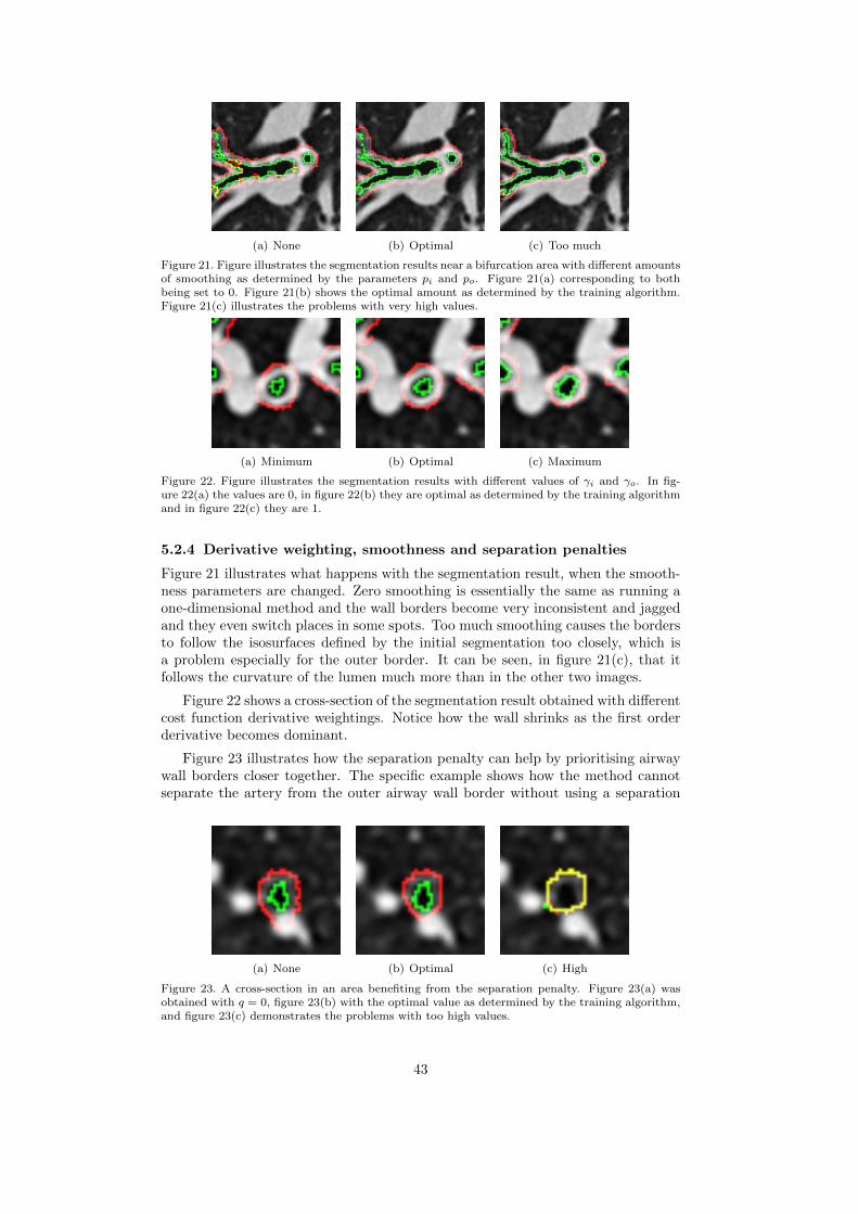
(a) None (b) Optimal (c) Too much
Figure 21. Figure illustrates the segmentation results near a bifurcation area with different amountsof smoothing as determined by the parameters pi and po. Figure 21(a) corresponding to bothbeing set to 0. Figure 21(b) shows the optimal amount as determined by the training algorithm.Figure 21(c) illustrates the problems with very high values.
(a) Minimum (b) Optimal (c) Maximum
Figure 22. Figure illustrates the segmentation results with different values of γi and γo. In fig-ure 22(a) the values are 0, in figure 22(b) they are optimal as determined by the training algorithmand in figure 22(c) they are 1.
5.2.4 Derivative weighting, smoothness and separation penalties
Figure 21 illustrates what happens with the segmentation result, when the smooth-ness parameters are changed. Zero smoothing is essentially the same as running aone-dimensional method and the wall borders become very inconsistent and jaggedand they even switch places in some spots. Too much smoothing causes the bordersto follow the isosurfaces defined by the initial segmentation too closely, which isa problem especially for the outer border. It can be seen, in figure 21(c), that itfollows the curvature of the lumen much more than in the other two images.
Figure 22 shows a cross-section of the segmentation result obtained with differentcost function derivative weightings. Notice how the wall shrinks as the first orderderivative becomes dominant.
Figure 23 illustrates how the separation penalty can help by prioritising airwaywall borders closer together. The specific example shows how the method cannotseparate the artery from the outer airway wall border without using a separation
(a) None (b) Optimal (c) High
Figure 23. A cross-section in an area benefiting from the separation penalty. Figure 23(a) wasobtained with q = 0, figure 23(b) with the optimal value as determined by the training algorithm,and figure 23(c) demonstrates the problems with too high values.
43

(a) None (b) Gen. ≤ 11 (c) Gen. ≤ 11, Ψ = 0.01
Figure 24. The leak detection method of section 3.6. Images show the lumen resulting from theGσ=0.45 method coloured by generation numbers. Figure 24(a) contains all the branches obtainedfrom the initial segmentation, figure 24(b) only generation 0-11 and figure 24(c) only the branchesin generation 0-11 satisfying Ψ < 0.01. Note that the viewing-angle of the left-most image isdifferent from the centre and right-most, as the leak would otherwise block most of the airways.
Method pi po γi γo q2D 0.218 0.267 0.785 0.311 0.00569Sk=16,τ=2.5 0.119 0.458 0.996 0.555 0.000Pα=10−4,β=2 0.111 0.732 0.991 0.379 0.0394Pα=10−4,β=4 0.111 0.892 1.00 0.264 0.0342Gσ=0.45 0.119 0.141 0.992 0.594 0.0364
Table 3. Optimal parameters obtained during training of each of the methods. Note that thevalues of the 2D method are not directly comparable to the methods implemented as part of thisthesis, because of implementation differences.
penalty. It also demonstrates how the value must be determined just right, as a toohigh setting can cause the airway wall borders to be found on top of each other.
5.2.5 Leak detection
Figure 24 illustrates the effect of the simple leak detection method, described insection 3.6. Notice how the initial segmentation has leaked into the parenchyma infigure 24(a). The leak follows the side of the lung causing its dome-like appearance.Figure 24(b) reveals that just limiting the generations to less than 12, results in amuch better looking airway tree, but a leak can still be spotted bottom-centre. Usingthe leak detection method with a Ψ of 0.01 results in the airway tree in figure 24(c).The bottom-centre leak is gone, but so are some of the smallest branches. Ψ = 0.01was chosen based on such examinations of a few segmentations with leaks, and itwas used in the rest of the experiments in this thesis.
5.3 Training
Table 3 show the optimal parameters obtained in the training of each of the meth-ods. Most of them are relatively similar, which is an indication that this way oftraining the parameters, makes sense. There are however some notable differences aswell. For instance Sk=16,τ=2.5 have 0 separation penalty and the outer smoothnesspenalty varies relatively much from method to method. To make sure that thesechoices were not the result of some local minima and associated with real differ-ences in the methods, every method was trained again with the optimal parametersof the other methods as initial values, and this did not lead to large changes inthe choice of parameters. We have no explanation for why the Sk=16,τ=2.5 methodapparently works the best with no separation penalty, however we think that theouter smoothness penalty and the regularisation used to calculate the columns arerelated, in such a way that more regularisation seem to be associated with a choiceof higher smoothness penalties. To understand why this might be, it is importantto understand that the initial segmentation is actually a segmentation of the lumen.
44

Part 2D Sk=16,τ=2.5 Pα=10−4,β=2 Gσ=0.45
Columns (s) - 11.7 529 109Minimum cut (s) - 4.11 27.2 9.89Total (s) 149 73 639 183Memory (GB) 0.31 1.2 2.9 1.8Graph vertices (×106) - 3.6 9.0 5.4Graph edges (×106) - 25 63 38
Table 4. Time to do the column construction process. For instance in the Sk=16,τ=2.5 case thiswould be the calculation of the medial axes and normals. In the Pα=10−4,β=2 and Gσ=0.45 casesthis would be the convolution with the kernels and flow line computations. Listed are also thetime to do the minimum cut calculation and the total, which includes construction of meshes andvoxelisation of the segmentation results.
2D Sk=16,τ=2.5 Pα=10−4,β=2 Pα=10−4,β=4 Gσ=0.45
0.124± 0.091 0.142± 0.077 0.120± 0.079 0.123± 0.080 0.111± 0.059
Table 5. The results of different methods and kernels on the test data set. Mean ± standarddeviation as given by equation 65.
The orientation and curvature of the lumen surface is different from the outer air-way wall border near bifurcations. At bifurcations, the lumen becomes separatedinto two new branches before the airway walls do, but increasing the regularisation,causes such lumen to ’melt’ together, making the orientation and curvature of thesesurfaces more like the outer airway border, which increases the usefulness of theouter smoothness penalty.
5.4 Performance
The programs were run on an Intel I7-920 at 2.67 GHz with 12 GB of ram. It shouldbe noted that implementations were not particularly optimised and the computa-tions were not parallelised. The numbers in table 5.4 are averages obtained on the7 airways in the test data set with the optimal parameters. The differences betweenthe Sk=16,τ=2.5, Pα=10−4,β=2 and Gσ=0.45 methods in time to calculate the minimumcut and memory usage are mostly due to differences in column length. Columns canprobably be shortened, which would likely equalise the numbers without changingthe segmentation results much.
The most interesting conclusion is that the three-dimensional methods are notmuch slower than the 2D method. This is likely due to complexities in resamplingthe images into a lot of two-dimensional slices. These two-dimensional slices areoften much bigger than they need to be because of uncertainties in calculatingbranch diameters from the initial segmentation. Also note the much faster columnconstruction of the method using the Gaussian kernel compared to the kernel basedon the electric field strength, partly due to its separability.
5.5 Comparison with manual segmentations
Table 5.5 shows the results of the comparisons with the manual segmentations inthe test data set, for each of the investigated methods using the optimal parameters.The flow line method using a Gaussian kernel with σ = 0.45 achieves the best resultand the method using medial axes columns with k = 16 neighbours to define themedial axes performs the worst. It is interesting to note that Gσ=0.45 actuallyperforms statistically better p < 0.05 than any of the other methods, and also hasa significantly lower variance in the quality of the results (p < 0.0001). This is anindication, that not only is it the best performing method, it is also less likely tobreak down, as described in section 3.5.1.
45

(a) 2D (b) Gσ=0.45
Figure 25. Figure 25(a) is an example cross-section of a segmentation break down of the 2D method,caused by only using two-dimensional information to infer the outer airway wall border position.Figure 25(b) illustrates how the Gσ=0.45 method more correctly segments it.
(a) Sk=16,τ=2.5 (b) Gσ=0.45
Figure 26. Cross-sections extracted near a branching area with segmentations obtained from theSk=16,τ=2.5 method in figure 26(a) and from the Gσ=0.45 method in figure 26(b)
.
The biggest advantage of the implemented three-dimensional methods comparedto the 2D method, is their ability to use all three dimensions of information to inferthe position of the surfaces. This was visible in the extracted two-dimensional cross-sections, in which the 2D method’s tendency to include other nearby structures wasapparent. Figure 25 is such an example, notice how the large abutting structuregets included in the 2D method’s segmentation, whereas Gσ=0.45 is able to morecorrectly place the outer airway wall border. The tendency also likely explains thehigher degree of variation observed in the segmentation results of this method.
We investigated the cross-sections segmented by the straight normal methodSk=16,τ=2.5 and it seems as if the method’s poor performance can be explained bytwo major problems. Poor quality normals and an inability to correctly handle thehigh curvature in bifurcation regions, as also predicted in section 2.2.6. The firstproblem results in some very erratic looking segmentations with spikes and evenholes, which cannot be explained by the image’s intensity function. The secondmakes the method very unlikely to correctly segment the area between two veryclose branches. We found these places to be full of holes, probably caused byself intersections or too short normals. See figure 26 for an example of both ofthese issues. Notice how the outer airway wall border segmentation obtained withSk=16,τ=2.5 collapses onto the inner airway wall border in the area between the twobranches.
The reason the electric field strength inspired kernels Pα=10−4,β∈{2,4} performedworse than the tested Gaussian kernel was less clear. In fact manually investigatingthe generated cross-sectional images revealed only small consistent differences inareas between two very close airways. Here the Pα=10−4,β∈{2,4} methods often hada few small holes where the Gσ=0.45 method had none. We think this is an indication
46
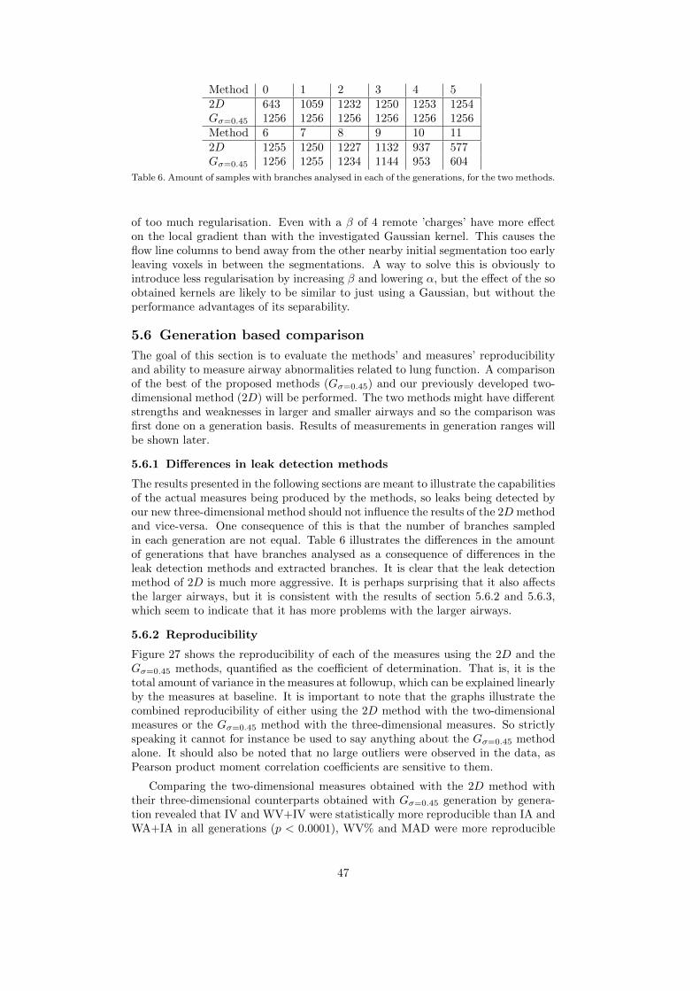
Method 0 1 2 3 4 52D 643 1059 1232 1250 1253 1254Gσ=0.45 1256 1256 1256 1256 1256 1256Method 6 7 8 9 10 112D 1255 1250 1227 1132 937 577Gσ=0.45 1256 1255 1234 1144 953 604
Table 6. Amount of samples with branches analysed in each of the generations, for the two methods.
of too much regularisation. Even with a β of 4 remote ’charges’ have more effecton the local gradient than with the investigated Gaussian kernel. This causes theflow line columns to bend away from the other nearby initial segmentation too earlyleaving voxels in between the segmentations. A way to solve this is obviously tointroduce less regularisation by increasing β and lowering α, but the effect of the soobtained kernels are likely to be similar to just using a Gaussian, but without theperformance advantages of its separability.
5.6 Generation based comparison
The goal of this section is to evaluate the methods’ and measures’ reproducibilityand ability to measure airway abnormalities related to lung function. A comparisonof the best of the proposed methods (Gσ=0.45) and our previously developed two-dimensional method (2D) will be performed. The two methods might have differentstrengths and weaknesses in larger and smaller airways and so the comparison wasfirst done on a generation basis. Results of measurements in generation ranges willbe shown later.
5.6.1 Differences in leak detection methods
The results presented in the following sections are meant to illustrate the capabilitiesof the actual measures being produced by the methods, so leaks being detected byour new three-dimensional method should not influence the results of the 2D methodand vice-versa. One consequence of this is that the number of branches sampledin each generation are not equal. Table 6 illustrates the differences in the amountof generations that have branches analysed as a consequence of differences in theleak detection methods and extracted branches. It is clear that the leak detectionmethod of 2D is much more aggressive. It is perhaps surprising that it also affectsthe larger airways, but it is consistent with the results of section 5.6.2 and 5.6.3,which seem to indicate that it has more problems with the larger airways.
5.6.2 Reproducibility
Figure 27 shows the reproducibility of each of the measures using the 2D and theGσ=0.45 methods, quantified as the coefficient of determination. That is, it is thetotal amount of variance in the measures at followup, which can be explained linearlyby the measures at baseline. It is important to note that the graphs illustrate thecombined reproducibility of either using the 2D method with the two-dimensionalmeasures or the Gσ=0.45 method with the three-dimensional measures. So strictlyspeaking it cannot for instance be used to say anything about the Gσ=0.45 methodalone. It should also be noted that no large outliers were observed in the data, asPearson product moment correlation coefficients are sensitive to them.
Comparing the two-dimensional measures obtained with the 2D method withtheir three-dimensional counterparts obtained with Gσ=0.45 generation by genera-tion revealed that IV and WV+IV were statistically more reproducible than IA andWA+IA in all generations (p < 0.0001), WV% and MAD were more reproducible
47
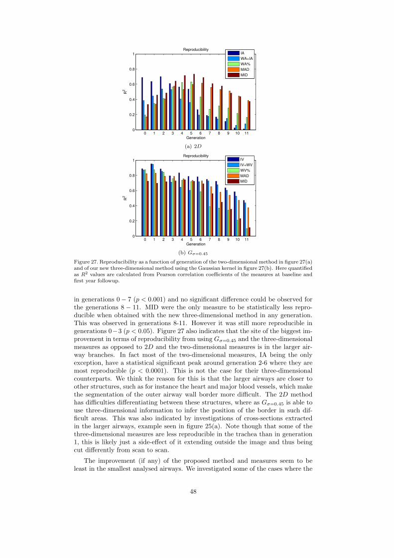
0 1 2 3 4 5 6 7 8 9 10 110
0.2
0.4
0.6
0.8
1
Generation
R2
Reproducibility
IA
WA+IA
WA%
MAD
MID
(a) 2D
0 1 2 3 4 5 6 7 8 9 10 110
0.2
0.4
0.6
0.8
1
Generation
R2
Reproducibility
IV
IV+WV
WV%
MAD
MID
(b) Gσ=0.45
Figure 27. Reproducibility as a function of generation of the two-dimensional method in figure 27(a)and of our new three-dimensional method using the Gaussian kernel in figure 27(b). Here quantifiedas R2 values are calculated from Pearson correlation coefficients of the measures at baseline andfirst year followup.
in generations 0− 7 (p < 0.001) and no significant difference could be observed forthe generations 8 − 11. MID were the only measure to be statistically less repro-ducible when obtained with the new three-dimensional method in any generation.This was observed in generations 8-11. However it was still more reproducible ingenerations 0−3 (p < 0.05). Figure 27 also indicates that the site of the biggest im-provement in terms of reproducibility from using Gσ=0.45 and the three-dimensionalmeasures as opposed to 2D and the two-dimensional measures is in the larger air-way branches. In fact most of the two-dimensional measures, IA being the onlyexception, have a statistical significant peak around generation 2-6 where they aremost reproducible (p < 0.0001). This is not the case for their three-dimensionalcounterparts. We think the reason for this is that the larger airways are closer toother structures, such as for instance the heart and major blood vessels, which makethe segmentation of the outer airway wall border more difficult. The 2D methodhas difficulties differentiating between these structures, where as Gσ=0.45 is able touse three-dimensional information to infer the position of the border in such dif-ficult areas. This was also indicated by investigations of cross-sections extractedin the larger airways, example seen in figure 25(a). Note though that some of thethree-dimensional measures are less reproducible in the trachea than in generation1, this is likely just a side-effect of it extending outside the image and thus beingcut differently from scan to scan.
The improvement (if any) of the proposed method and measures seem to beleast in the smallest analysed airways. We investigated some of the cases where the
48
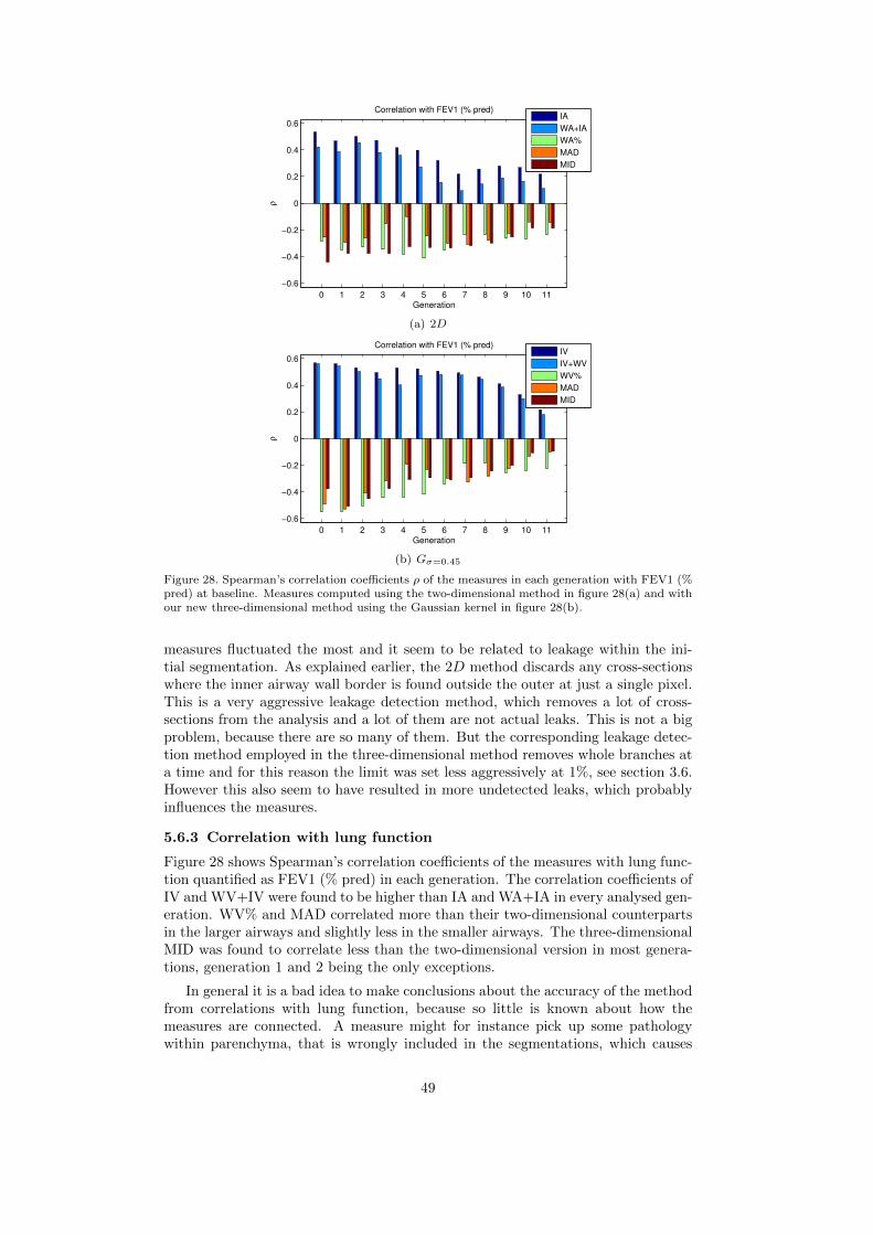
0 1 2 3 4 5 6 7 8 9 10 11
−0.6
−0.4
−0.2
0
0.2
0.4
0.6
Generation
ρ
Correlation with FEV1 (% pred)
IA
WA+IA
WA%
MAD
MID
(a) 2D
0 1 2 3 4 5 6 7 8 9 10 11
−0.6
−0.4
−0.2
0
0.2
0.4
0.6
Generation
ρ
Correlation with FEV1 (% pred)
IV
IV+WV
WV%
MAD
MID
(b) Gσ=0.45
Figure 28. Spearman’s correlation coefficients ρ of the measures in each generation with FEV1 (%pred) at baseline. Measures computed using the two-dimensional method in figure 28(a) and withour new three-dimensional method using the Gaussian kernel in figure 28(b).
measures fluctuated the most and it seem to be related to leakage within the ini-tial segmentation. As explained earlier, the 2D method discards any cross-sectionswhere the inner airway wall border is found outside the outer at just a single pixel.This is a very aggressive leakage detection method, which removes a lot of cross-sections from the analysis and a lot of them are not actual leaks. This is not a bigproblem, because there are so many of them. But the corresponding leakage detec-tion method employed in the three-dimensional method removes whole branches ata time and for this reason the limit was set less aggressively at 1%, see section 3.6.However this also seem to have resulted in more undetected leaks, which probablyinfluences the measures.
5.6.3 Correlation with lung function
Figure 28 shows Spearman’s correlation coefficients of the measures with lung func-tion quantified as FEV1 (% pred) in each generation. The correlation coefficients ofIV and WV+IV were found to be higher than IA and WA+IA in every analysed gen-eration. WV% and MAD correlated more than their two-dimensional counterpartsin the larger airways and slightly less in the smaller airways. The three-dimensionalMID was found to correlate less than the two-dimensional version in most genera-tions, generation 1 and 2 being the only exceptions.
In general it is a bad idea to make conclusions about the accuracy of the methodfrom correlations with lung function, because so little is known about how themeasures are connected. A measure might for instance pick up some pathologywithin parenchyma, that is wrongly included in the segmentations, which causes
49
the correlation coefficients to rise. Even more likely, wrong segmentations couldbe caused by pathology, which could make a less stable algorithm more sensitiveto disease progression. When that is said, it is important to establish that we arenot just measuring something irrelevant very consistently and the conclusion fromthe data displayed in figure 28 is that we are not. The lung function correlationcoefficients seem to tell a similar story as the reproducibility measurements in theprevious section. That is, that the newly proposed three-dimensional method andmeasures for the most part result in measurements, that are more correlated withlung function than our previously developed two-dimensional method9 and that thiscorrelation increase is most apparent in the larger airways.
Another interesting observation, which we will discuss in section 6.2.1, is thatespecially IV and WV+IV seem to gain the most when compared with the two-dimensional versions.
5.7 Per scan measures
The purpose of this section is to show results of the measures obtained in branchgeneration ranges, and to illustrate that this way of combining measurements takenthroughout the airway tree into one single measure makes sense. Additionally a com-parison of the new three-dimensional algorithm with the previous two-dimensionalmethod will be performed with the so obtained measures.
It is important to note, before we go any further with this analysis, that achoice of generation range is not just a matter of getting the highest correlationwith lung function or reproducibility, as the relationship between airway measuresand lung function is fairly complex with many covariates.57 As such, the method ofcombining the measures from different sites in the airway should ideally be based ona detailed statistical analysis, covariates should be included, and the results shouldbe verified on an independent data set. A future study could look into this.
5.7.1 Reproducibility and correlation with lung function
Measures obtained with the 2D method have previously been established to cor-relate most with lung function and be most reproducible in the generation range3-11.57 This does not seem to be the case with the new method, judging by resultsof section 5.6.2 and 5.6.3. Because the new method is able to segment the largerairways even better than the airways of medium size, maybe the choice of generationrange should be based just as much on the capability of the airway segmentationand tree extraction algorithm to consistently extract the branches. A generationrange of 1-6 for instance would mean that roughly 80% of the branches would becorrectly found and included in the analysis and there would only be an averagevariation in this number of at most 16% in any specific generation, see figure 19.The trachea should be ignored because it was not included in its entirety in theimages.
Figure 29 show the reproducibility and lung function correlation coefficientsof the 2D method over the previously established optimal range of 3-11 and theproposed method in the ranges 3− 11, 3− 6 and 1− 6. It is interesting that even inthe range of 3−11 where the 2D method works the best the newly proposed methodproduces measures of MAD, WV%, IV+WV and IV that are more (p < 0.001) andin the case of MID equally reproducible to the two-dimensional measures. The three-dimensional measures also correlated more with lung function, the only exceptionsbeing MID and WV%, which correlate just slightly less than their two-dimensionalcounterparts. Changing the generation range interval over 3−6 to 1−6 increases thereproducibility of the three-dimensional measures further and the absolute valuesof the lung function correlation coefficients of every measure become larger than
50

MAD MID WV% \ WA% IV+WV \ WA+IA IV \ IA0
0.2
0.4
0.6
0.8
1
R2
2D 3−11
Gσ = 0.45
3−11
Gσ = 0.45
3−6
Gσ = 0.45
1−6
(a) Reproducibility
MAD MID WV% \ WA% IV+WV \ WA+IA IV \ IA−0.6
−0.4
−0.2
0
0.2
0.4
0.6
0.8
ρ
2D 3−11
Gσ = 0.45
3−11
Gσ = 0.45
3−6
Gσ = 0.45
1−6
(b) Lung function
Figure 29. Reproducibility of the 2D method measures sampled in range 3-11 and the Gσ=0.45
method measures sampled in ranges 3-11, 3-6 and 1-6 shown in figure 29(a). Correlation with lungfunction for the same methods, measures and generation ranges shown in figure 29(b).
the corresponding absolute values of the correlation coefficients obtained with thetwo-dimensional measures.
The reproducibility of FEV1 (% pred) within this data set was 0.87, which meansthat is statistically higher than all the measures, except IV (p < 0.05) in all thesampled generation ranges and IV+WV in 1 − 6. IV is actually statistically morereproducible in the generation range 1− 6 than FEV1 (% pred).
We note that the reproducibility of these per scan measures generally do notbecome better than what is seen in generation 1 alone for instance. No generaltrend of larger lung function correlation coefficients can be observed either. Howeverthey may capture changes to a larger part of the airway without being much lessreproducible than measures obtained in any single generation. It also seems likelygiven that we know COPD mostly affects the smaller airways that they betterrepresent the true abnormalities caused by COPD and not just covariates.
5.7.2 COPD Diagnostic ability
Figure 30 shows the diagnostic ability of the methods and measures calculated in ageneration range of 3−11. The AUC values of IV at stage 1 and 2, IV+WV at stage1, 2 and 3 and MAD at stage 1 and 2 were all statistically larger than their two-dimensional counterparts (p < 0.05), whereas WV% was found to be statisticallysmaller in all stages (p < 0.05). No statistically significant difference was foundwithin the rest of the measures. Although the results are not completely clear,a majority of the measures does show larger AUC values with the new method
51

> 0 > 1 > 20.5
0.55
0.6
0.65
0.7
0.75
0.8
0.85
Stage
AU
C
IA
WA+IA
WA%
MAD
MID
(a) 2D
> 0 > 1 > 20.5
0.55
0.6
0.65
0.7
0.75
0.8
0.85
Stage
AU
C
IV
IV+WV
WV%
MAD
MID
(b) Gσ=0.45
Figure 30. Diagnostic ability of the methods and measures quantified as AUC. Differentiatingbetween subjects suffering from the disease and not (> 0), subjects with stage 2 and worse (> 1)and subjects with stage 3 and worse (> 2). Measures computed with the 2D and Gσ=0.45 methodsare shown in figure 30(a) and figure 30(b) respectively.
MAD MID WV% IV+WV IV0
0.2
0.4
0.6
0.8
1
R2
Bifurcation
Non−bifurcation
(a) Reproducibility
MAD MID WV% IV+WV IV−0.4
−0.2
0
0.2
0.4
0.6
ρ
Bifurcation
Non−bifurcation
(b) Lung function
Figure 31. Reproducibility and correlation with lung function inside and outside bifurcation re-gions.
than with the previous method. The increases are also numerically much largerthan the decreases. Again the largest improvements seem to be with the measuresquantifying lumen and total airway size, IV and IV+WV.
We investigated the AUC values of the measures obtained with Gσ=0.45 in thegeneration ranges 3-6 and 1-6 as well (results not shown), however the larger lungfunction correlation coefficients and improved reproducibility observed in theseranges, does not seem to equate to better diagnostic ability. Perhaps this is anindication that the smaller airways are important, despite the lower accuracy andprecision associated with measuring them.
5.7.3 Bifurcation regions
Figure 31 shows reproducibility and Spearman’s correlation coefficient of the mea-sures with FEV1 (% pred) inside and outside bifurcation regions. No significant dif-ference was observed in reproducibility between the bifurcation and non-bifurcationregions using the measures MAD, MID, WV%, IV+WV, IV and a significance levelof 0.05. This indicates that the proposed method is equally reproducible inside andoutside bifurcation regions. The lung function correlation coefficients are also verysimilar, which is evidence to suggest that airway abnormalities caused by COPD arenot more or less prevalent in bifurcation regions. Further investigations will haveto establish whether measurements in the bifurcation and non-bifurcation regionsare independent and thus complement each other.
5.7.4 St. George’s Respiratory Questionnaire
Figure 32 show Spearman’s rho of FEV1 (% pred) and each of the three-dimensionalairway abnormality measures with the SGRQ components. Most of the coefficientsindicate moderate links between the measures and how questionnaires were com-pleted. Especially how subjects perceive their symptoms and what impact the
52

Health Impacts Symptoms Activity Total−0.25
−0.2
−0.15
−0.1
−0.05
0
0.05
0.1
0.15
0.2
0.25
ρ
IV
IV+WV
WV%
MAD
MID
FEV1(%PRED)
Figure 32. Significant Spearman’s rank correlation coefficients of each of the three-dimensionalairway abnormality measures and FEV1 (% pred) with the SGRQ component scores (Impacts,Symptoms and Activity), total score (Total) and the extra posed question on subject health(Health).
disease has on their daily lives were found to be related to the analysed abnormal-ity measures. WV%, MAD and MID were found to be positively correlated withthe components, meaning that an increase in wall volume relative to the completeairway area, an increase in mean airway density or mean inner volume density wereassociated with a decrease in health status and perceived well being. The oppositewas true for IV and IV+WV, meaning that a smaller lumen volume or airway vol-ume were found to be associated with negative health effects. IV+WV was howevernot found to be significantly correlated with the activity component. These areall results that fall well in line with current theory, saying that COPD leads to anincrease in mass within the airway walls and narrowed airways, which causes healthproblems. The figure also shows that out of the analysed measures, WV%, MADand MID are likely the best airway indicators of subject health and perceived wellbeing as quantified by SGRQ.
Figure 32 also shows that even the answer to the simple question of how subjectsdescribe their current health is significantly correlated with airway abnormalities,specifically IV+WV, MAD and MID. This reflects the relationship, already indi-cated by the SGRQ components, that higher values of mean airway density, innervolume density or a lower airway volume are associated with a worse health status.
6. DISCUSSION
6.1 Medial axes and normal directions from Delaunay balls
It should be noted, that the problem of obtaining normals to discrete representationsof continuous surfaces can be approached in many different ways and we have notinvestigated the subject in detail. However from the experience and results obtainedwithin this work it seems to us that the method of reference 66 is more applicable toactual noisy point clouds and not, as in this problem, connected meshes of verticesobtained from an already rather correct segmentation of the lumen.33 The errorsin our case are probably not as much noise as discretisation effects.
We think that our mesh choice is a likely contributing factor to these problems,as it directly reflects the voxels of the initial segmentation. Some Delaunay ballswill undoubtedly be very small due to its step-like nature. We do not think trian-gulations, such as those obtained with the popular marching cubes algorithm77 aresolutions to these problems, as they still directly reflect the discrete surface. Wehave experienced a little with pre-smoothing the surface, as done in reference,79
53

instead with better results. Surface smoothing however can change the topology ofthe surface, and the objects shrink as a result.
Another more complicated solution could be to use a level set method69 to obtainan implicit representation of the initial segmentation surface, and then create a meshfrom this. This implicit surface representation could be used to estimate the medialaxes93 and normals more precisely.
Another interesting work uses parabolic partial differential equations to extractthe medial axes from mesh representations, the method is robust to noise becauseof the diffusion equation used, which smoothes the result. Unfortunately it seemsslow judging from the reported results.94
6.2 Two versus three-dimensional methods
It is interesting that the two-dimensional method work so well compared to theanalysed three-dimensional methods, see Table 5.5. It can probably in part be ex-plained by the comparison being done with two-dimensional data, which is likely tobe biased toward a two-dimensional method. There is also a bias favouring the two-dimensional method, in that any other airway within the cross-section not correctlymarked ’to be excluded’, see the blue areas in figure 18(b), will count as errors inthe three-dimensional methods, but not in the two-dimensional method. There isalso a quality in the three-dimensional methods, not reflected in the comparison,in that they do not require an accurate extraction of centred perpendicular cross-sections to work properly, but two-dimensional methods do. However both typesof methods suffer from this in the comparison, as the training set is build on suchcross-sections.
When all this is said, we still think there is evidence to say that the two-dimensional method in accuracy is at least comparable to Sk=16,τ=2.5. One mightconsider why this is so, given that three-dimensional methods should be able toutilise one more dimension of coherency in the data, and thus better be able tohandle areas where the wall borders are weakly defined. We think that one rea-son might be that the smoothness penalties implemented by the two-dimensionalmethod better captures the structure of the human airways. That is, it might bebetter to penalise deviance from some idealised circular/tubular structure than fromthe surface curvature of some voxelised initial segmentation. The first probably cap-tures some general knowledge of the human airways, whereas the last, because it isgenerated from the same volume of data, is probably too specific and thus becomessensitive to noise, mucus and other artefacts not reflecting the true nature of theairway.
This lead us to the conclusion, that a graph construction scheme based on con-necting the inter column edges using the euclidean distance between column vertices,rather than how far they are from the initial surface, could improve our segmenta-tion results. Such a scheme would prefer straighter surfaces in the euclidean sense,rather than surfaces following the isosurfaces in the convoluted images.
6.2.1 Measure differences
IV and IV+WV are the measures, which benefit the most from the proposed Gσ=0.45
method compared to the two dimensional versions, both in terms of reproducibility,increased correlation with lung function and diagnostic ability. This indicate animprovement in the segmentation method, given that these two measures directlyquantify the segmented volumes and areas. There are however also other explana-tions for this. The branch volume could remain more constant than branch widthduring inspiration and expiration effects. For instance if these effects vary from
54

elongation and thinning during inspiration to shortening and widening during expi-ration. We also know, from previous investigations,57 that the airway segmentationmethod is sensitive to pathology in such a way that sicker subjects have fewer suc-cessfully segmented branches. This enhances the association between the measuresand the disease, an enhancement, which is likely to be even more present in thevolume measures.
7. CONCLUSION
The motivation for solving the problem of segmenting human airway walls in CTimages was described with focus on applications within COPD analysis and diag-nosis.
Previous methods were described, reflected on and evaluated. Starting withsimple one-dimensional methods, such as FWHM, over more sophisticated two-dimensional methods, using constraints and penalties to enforce solution coherency,to the most advanced methods of today, which are able to accurately and preciselydetermine the position of the airway wall borders in three dimensions. The methods’theory and purpose in practice were accounted for with a special emphasis on graphcut methods.
We have suggested new methods for solving the problem, by combining the air-way segmentation method of reference 33 and the tree extraction method describedin reference 28 with a novel graph construction technique, whose non-intersectingcolumns follow greatest ascent and descent flow lines within a continuous functioncalculated from the airway segmentation. An optimal solution was obtained usingthe maximum flow graph of reference 9. The method was inspired by the electriclines of force columns initially described in reference 2. We have documented howsuch columns can be calculated using simple convolutions, and that the Gaussiankernel could be a better choice than a kernel based on the electric field strength. Wehave furthermore shown how solutions obtained using the maximum flow graph ofreference 9 relates to the optimal net family of methods and that a subset of the opti-mal VCE-weight net problems specified on proper ordered multi-column graphs, canbe solved more efficiently using it. Additionally, a method using straight columnspointing in the normal direction and calculated using an approximation to the me-dial axes, similarly to reference 4, was documented and implemented as a referencemethod.
The methods were applied on data from the DLCST and CBQ. 649 cross-sectional images were extracted randomly from the airways of 15 subjects andmanually segmented. The data set was then split randomly in a training and anindependent test data set. Optimal values of method parameters were found usingthe training data set and quantitatively and qualitatively evaluated on the test dataset. The proposed method using non-intersecting flow line columns calculated witha Gaussian kernel was found to be statistically superior in terms of mean segmenta-tion relative area of overlap to the same method using flow line columns calculatedfrom kernels based on the electric field strength, the method using straight columnsand a previously developed two-dimensional method.9
Additionally a large scale comparison of the proposed method and the pre-viously developed two-dimensional methods’ COPD diagnostic abilities were per-formed. Airway abnormality measures obtained with the two methods were eval-uated on reproducibility, using the coefficient of determination, calculated fromPearson product moment correlation coefficients, correlation with lung function,using Spearman’s rank correlation coefficient of the measures and FEV1 (% pred),and diagnostic ability in the form of AUC values of each measure in the three first
55
disease stages. IV and IV+WV were found to be more reproducible in all exam-ined generations (0-11) than similar two-dimensional measures computed using thepreviously developed two-dimensional method (p < 0.0001). WV% and MAD weresimilarly found to be more reproducible in generations 0-7 (p < 0.001) and no statis-tical difference was observed in the range 8-11, whereas MID was found to be morereproducible in generations 0-3 and less reproducible from 8-11 (p < 0.05). Theproposed method also enabled measures that as a majority correlated more withlung function than similar measures obtained with the two-dimensional method.IV and IV+WV were found to correlate more in every examined generation, WV%and MAD correlated more in the larger and slightly less in the smaller airways,and MID was found to correlate less in most generations. Measures obtained withthe proposed method in the branch generation range 3-11, previously found to bethe best range for the two-dimensional method, were in the case of MAD, WV%,IV+WV and IV found to be more reproducible (p < 0.001), whereas no significantchange could be observed for MID. The three-dimensional measures were also foundto correlate more with lung function, with the exception of MID and WV%, whichcorrelated just slightly less. The diagnostic ability of the measures obtained withthe proposed method were for the most part better. IV had significantly higherAUC values in stage 1 and 2, IV+WV in stage 1, 2 and 3 and MAD at stage 1 and2 (p < 0.05). WV% was found to be statistically worse in every examined stage(p < 0.05).
We also investigated, whether the bifurcation regions, which the previous two-dimensional method for the most part could not segment, were more or less influ-enced by the disease. The results show that the method is able to segment theseareas with just as high reproducibility as the non-bifurcation regions (p < 0.05).The lung function correlation coefficients inside and outside these regions were alsofound to be very similar, indicating that airway abnormalities caused by COPD areneither less nor more prevalent in bifurcation areas.
The relationship between airway abnormality measures and how subjects per-ceive their health was investigated using the SGRQ. WV%, MAD and MID werefound to be positively correlated with the SGRQ components, whereas IV andIV+WV were found to be negatively correlated (p < 0.05). We found that es-pecially symptoms and what impact the disease had on their social functioningwere related to airway abnormalities and that WV%, MAD and MID are likely thebest indicators of subject health and perceived well being as quantified by SGRQanswers.
In general the results obtained from the work in this thesis are well in line withcurrent theory, saying that COPD leads to an increase in mass within the airwaywalls and narrowed airways, which causes poorer lung function and other healthproblems. Results indicate that this increase in mass, can be quantified using thethree-dimensional measures: the wall volume percentage, the mean airway densityand the mean inner volume density. The narrowing can similarly be quantified usingthe inner volume and the total airway volume.
Even though measurements for the most part do not match basic spirometry inreproducibility, they do enable localization of the disease within the lungs, makingit possible for instance to link symptoms with disease phenotypes. The results pre-sented demonstrate the use of CT and the proposed method for COPD investigationand diagnosis.
We therefore conclude that we have fulfilled the goals set out in the projectdescription.
56

8. FUTURE WORK
8.1 Improved leak detection
It is our opinion that removing leaks or erroneous areas in the initial segmentation, isone of the most important issues for improving measurement accuracy and precision.
The issue could be approached, for instance by building a reference of knownleaks and accepted branches. It is possible that the Exact’0928 database could beused for this. Using this reference a leak classifier could be build, perhaps usingairway wall measurements as feature descriptors. This classifier could be used toobtain weights describing how believable a segmentation of any given branch was.
8.2 Parallelisation
Within this work a graph resolution of 0.5 mm was used, meaning the initial surfaceand the columns were sampled at a 0.5 mm spacing. This was done because higherresolutions, simply lead to unacceptable computation times. Experiments withresolutions of 1 mm showed much worse results and thus extrapolating leads tothe conclusion that higher resolutions than 0.5 mm, might equate to even betterresults. To properly investigate this, the computation time and memory usage ofthe algorithm will have to be improved.
The algorithmic running time of the method is dominated by the used maximumflow algorithm. As mentioned, many algorithms exist and their worst case runningtimes differ. The Boykov-Kolmogorov62 algorithm we used in this thesis has a worstcase running time of O(|E||V |2|C|), where |V | is the number of vertices, |E| is thenumber of edges and |C| is the cost of the minimum cut. So there is a lot to begained if the graph could somehow be made smaller.
It is not likely that a graph representing the complete airway tree is needed tocorrectly segment for instance the trachea. In fact, it should be possible to measurehow much the influence of given vertices and edges on the minimum cut decreaseswith distance in the graph. Such measurements could be used to split the graph insmaller parts, which individually would be faster to solve and require less memory.
8.3 Repetitive approach
The proposed method is very sensitive to the accuracy of initial segmentation.Mostly because the columns, for accuracy and performance reasons, need to berather well resolved and short. It is possible that a repetitive approach could im-prove on this sensitivity, by perhaps evolving the surfaces in iterations, startingwith longer columns with more widely spaced vertices and working towards smallercolumns with closer spaced vertices as the solution converged. It is likely that theconvolution kernels would have to use more regularization in the first iterations andthis could then be lowered with iterations, using common concepts from scale spacetheory.
Before this is possible, some work would have to be done, on how to connectthe two surfaces between iterations. We would also need to establish that multipleiterations actually converge to a solution.
57

APPENDIX A. ALGORITHMS
A.1 Normal and feature size algorithms
Assuming the existence of the following functions:
Points(M) Returns the vertices of a mesh M .Delaunay(P ) Finds the Delaunay triangulation of a point
set P .Nearest(P , k, p) Finds the k nearest neighbours in a point set
P to p.LargestBall(D, p) Given a Delaunay triangulation D, returns
the largest Delaunay ball incident to a pointp.
LargestInsideBall(M , D, p) Given a Delaunay triangulation D, returnsthe largest Delaunay ball incident to a pointp inside the mesh M .
LargestOutsideBall(M , D, p) Given a Delaunay triangulation D, returnsthe largest Delaunay ball incident to a pointp outside the mesh M .
Radius(B) Return the radius of a ball B.Centre(B) Return the centre of a ball B.Distance(p0, p1) Return the euclidean distance between two
points p0 and p1.Distance(P , p) Return the euclidean distance from the point
p to the point set P .Outside(M , p) Returns true if the point p is outside the
mesh M .
Given a mesh M and an error tolerance τ , the following defines the normal calcu-lation algorithm in pseudocode:
Normals(M , τ)P ← Points(M)N ← NilE ← F ← {}D ← Delaunay(P )for each p ∈ P
m ← Nearest(P , 1, p)B ← LargestBall(D, p)if Radius(B) > τ Distance(m, p)
c ← Centre(B)n ←(c-p)/Distance(c, p)if Outside(M , c)
n ← −nN [p] ← nE ← E ∪ {p}
elseF ← F ∪ {p}
for each p ∈ Fq ← Nearest(E, 1, p)N [p] ← N [q]
return N
58

Given a neighbour search count k, the following defines the feature size algorithmin pseudocode:
Features(M , k)P ← Points(M)D ← Delaunay(P )Mi ← Mo ← {}for each p ∈ P
N ← Nearest(P , k, p)ri ← ro ← 0for each n ∈ N
Bi ← LargestInsideBall(M , D, n)if Radius(Bi) > ri
ri ← Radius(Bi)pi ← Centre(Bi)
Bo ← LargestOutsideBall(M , D, n)if Radius(Bo) > ro
ro ← Radius(Bo)po ← Centre(Bo)
Mi ← Mi ∪ {pi}Mo ← Mo ∪ {po}
Fi ← Fo ← Nilfor each p ∈ P
Fi[p] ← Distance(Mi, p)Fo[p] ← Distance(Mo, p)
return Fi, Fo
59

A.2 Training algorithm
Assuming the existence of some function Evaluate(P ) which runs the airway wallsegmentation method on the complete training set with the parameters P andreturns the sum of the errors of each involved cross-section as calculated in equa-tion 65, an initial set of randomized parameters P , error tolerances for each param-eter ε, left L and right R search interval limits and a maximum number of iterationsk. The pseudocode is given below:
Optimise(k, P, ε, L, R)Ep ← Evaluate(P)for i ← 0 to k
for j ← 0 to length(P)p ← P[j]l ← L[j], r ← R[j]while true
backup ← P[j]P[j] ← lEl ← Evaluate(P)P[j] ← rEr ← Evaluate(P)P[j] ← backup
if El < Erif El < Ep
Ep ← Elp ← lmoved ← truebreak
else if El > Erif Er < Ep
Ep ← Erp ← rmoved ← truebreak
if r-P[j] ≤ ε[j] and P[j]-l ≤ ε[j]break
l ← (P[j]+l)/2r ← (P[j]+r)/2
P[j] ← pif !moved
break
60

REFERENCES
[1] Wu, X. and Chen, D. Z., “Optimal net surface problems with applications,”in [ICALP ’02: Proceedings of the 29th International Colloquium on Au-tomata, Languages and Programming ], 1029–1042, Springer-Verlag, London,UK (2002).
[2] Yin, Y., Song, Q., and Sonka, M., “Electric field theory motivated graph con-struction for optimal medical image segmentation,” in [GbRPR ’09: Proceed-ings of the 7th IAPR-TC-15 International Workshop on Graph-Based Repre-sentations in Pattern Recognition ], 334–342, Springer-Verlag, Berlin, Heidel-berg (2009).
[3] Li, K., Millington, S., Wu, X., Chen, D. Z., and Sonka, M., “Simultaneoussegmentation of multiple closed surfaces using optimal graph searching,” in[IPMI’05: Proceedings of the 19th International Conference on InformationProcessing in Medical Imaging ], 406–417 (2005).
[4] Liu, X., Chen, D. Z., Wu, X., and Sonka, M., “Optimal graph-based segmenta-tion of 3d pulmonary airway and vascular trees across bifurcations,” in [FirstInternational Workshop on Pulmonary Image Processing ], 103–111 (2008).
[5] Heimann, T., Munzing, S., Meinzer, H.-P., and Wolf, I., “A shape-guided de-formable model with evolutionary algorithm initialization for 3d soft tissuesegmentation,” in [IPMI’07: Proceedings of the 20th international conferenceon Information processing in medical imaging ], 1–12, Springer-Verlag, Berlin,Heidelberg (2007).
[6] Yin, Y., Zhang, X., and Sonka, M., “Optimal multi-object multi-surface graphsearch segmentation: Full-joint cartilage delineation in 3d,” in [Proceedings ofthe 12th annual Conference on Medical Image Understanding and Analysis ],104–108 (2008).
[7] Kainmueller, D., Lamecker, H., and Zachow, S., “Multi-object segmentationwith coupled deformable models,” Annals of the British Machine Vision As-sociation (BMVA) 5, 1–10 (2009).
[8] Liu, X., Chen, D. Z., Tawhai, M., Hoffman, E., and Sonka, M., “Measurement,evaluation and analysis of wall thickness of 3D airway trees across bifurcations,”in [The Second International Workshop on Pulmonary Image Processing ], 161–171 (2009).
[9] Petersen, J., Lo, P., Nielsen, M., , Edula, G., Ashraf, H., Dirksen, A., andde Bruijne, M., “Quantitative analysis of airway abnormalities in CT,” in [Med-ical Imaging 2010: Computer-Aided Diagnosis. Edited by N. Karssemeijer; R.M. Summers. Proceedings of SPIE ], 7624 (2010).
[10] Pedersen, J. H., Ashraf, H., Dirksen, A., Bach, K., Hansen, H., Toennesen, P.,Thorsen, H., Brodersen, J., Skov, B. G., Døssing, M., Mortensen, J., Richter,K., Clementsen, P., and Seersholm, N., “The danish randomized lung cancerCT screening trial–overall design and results of the prevalence round.,” Journalof Thoracic Oncology 4, 608–614 (May 2009).
[11] Rabe, K. F., Hurd, S., Anzueto, A., Barnes, P. J., Buist, S. A., Calverley, P.,Fukuchi, Y., Jenkins, C., Rodriguez-Roisin, R., van Weel, C., and Zielinski, J.,“Global strategy for the diagnosis, management, and prevention of chronic ob-structive pulmonary disease: GOLD executive summary.,” American Journalof Respitory and Critical Care Medicine 176, 532–555 (September 2007).
[12] Hogg, J. C., Chu, F., Utokaparch, S., Woods, R., Elliot, W. M., Buzatu,L., Cherniack, R. M., Rogers, R. M., Sciurba, F. C., Coxson, H. O., andPare, P. D., “The nature of small-airway obstruction in chronic obstructivepulmonary disease,” The New England Journal of Medicine 350(26), 2645–2653 (2004).
61

[13] Ooi, G. C., Khong, P. L., Chan-Yeung, M., Ho, J. C. M., Chan, P. K. S., Lee, J.C. K., Lam, W. K., and Tsang, K. W. T., “High-resolution CT quantificationof bronchiectasis: clinical and functional correlation,” Radiology 225, 663–672(2002).
[14] Hillard, T. N., Regamey, N., Shute, J. K., Nicholson, A. G., Alton, E. W.F. W., Bush, A., and Davies, J. C., “Airway remodelling in children withcystic fibrosis,” Thorax 63, 1074–1080 (2007).
[15] Martınez, T. M., Llapur, C. J., Williams, T. H., Coates, C., Gunderman,R., Cohen, M. D., Howenstine, M. S., Saba, O., Coxson, H. O., and Tepper,R. S., “High-resolution computed tomography imaging of airway disease ininfants with cystic fibrosis,” American Journal of Respiratory and Critical CareMedicine 172, 1133–1138 (2005).
[16] Bousquet, J., Chanez, P., Lacoste, J. Y., White, R., Vic, P., Godard, P., andMichel, F. B., “Asthma: a disease remodeling the airways,” Allergy 47, 3–11(1992).
[17] Tockman, M. S., Anthonisen, N. R., Wright, E. C., and Donithan, M. G.,“Airways obstruction and the risk for lung cancer,” Annals of InternalMedicine 106(4), 512–518 (1987).
[18] Weibel, E. R., “What makes a good lung?,” Swiss Medical Weekly 139(27-28),375–86 (2009).
[19] Weinheimer, O., Achenbach, T., Bletz, C., Duber, C., Kauczor, H.-U., andHeussel, C. P., “About objective 3-D analysis of airway geometry in com-puterized tomography,” IEEE Transactions on Medical Imaging 27(1), 64–74(2008).
[20] Kiraly, A. P., Odry, B. L., Naidich, D. P., and Novak, C. L., “Boundary-specific cost functions for quantitative airway analysis,” in [MICCAI’07: Pro-ceedings of the 10th international conference on medical image computing andComputer-Assisted Intervention-Part I ], 784–791, Springer-Verlag, Berlin, Hei-delberg (2007).
[21] Estepar, R. S. J., Washko, G. G., Silverman, E. K., Reilly, J. J., Kikinis, R.,and Westin, C.-F., “Accurate airway wall estimation using phase congruency,”in [MICCAI’06: Proceedings of the Ninth International Conference on Med-ical Image Computing and Computer-Assisted Intervention-Part II ], 125–134(2006).
[22] Tschirren, J., Hoffman, E. A., McLennan, G., and Sonka, M., “Intrathoracicairway trees: segmentation and airway morphology analysis from low-dose CTscans,” IEEE Transactions on Medical Imaging 24(12), 1529–1539 (2005).
[23] Tschirren, J., Hoffman, E. A., McLennan, G., and Sonka, M., “Segmentationand quantitative analysis of intrathoracic airway trees from computed tomogra-phy images,” Proceedings of the American Thoracic Society 2, 484–487 (2005).
[24] Li, K., Wu, X., Chen, D. Z., and Sonka, M., “Efficient optimal surface detec-tion: theory, implementation, and experimental validation,” in [Medical Imag-ing 2004: Image Processing. Edited by Fitzpatrick, J. Michael; Sonka, Milan.Proceedings of the SPIE. ], 5370, 620–627 (2004).
[25] Li, K., Wu, X., Chen, D. Z., and Sonka, M., “Optimal surface segmentation involumetric images-a graph-theoretic approach,” IEEE Transactions on PatternAnalysis and Machine Intelligence 28(1), 119–134 (2006).
[26] Saragaglia, A., Fetita, C., Preteux, F., Brillet, P. Y., and Grenier, P. A., “Accu-rate 3d quantification of the bronchial parameters in MDCT,” in [MathematicalMethods in Pattern and Image Analysis. Proceedings of SPIE ], 5916 (2005).
62
[27] Saragaglia, A., Fetita, C., and Preteux, F., “Assessment of airway remodelingin asthma: Volumetric versus surface quantification approaches,” in [Medi-cal Image Computing and Computer-Assisted Intervention MICCAI 2006 ],Larsen, R., Nielsen, M., and Sporring, J., eds., Lecture Notes in ComputerScience 4191, 413–420, Springer Berlin / Heidelberg (2006).
[28] Lo, P., van Ginneken, B., Reinhardt, J. M., and de Bruijne, M., “Extractionof airways from CT (EXACT’09),” in [The Second International Workshop onPulmonary Image Analysis ], 175–189 (2009).
[29] Wiemker, R., Bulow, T., and Lorenz, C., “A simple centricity-based regiongrowing algorithm for the extraction of airways,” in [The Second InternationalWorkshop on Pulmonary Image Analysis ], (2009).
[30] Feuerstein, M., Kitasaka, T., and Mori, K., “Adaptive branch tracing andimage sharpening for airway tree extraction in 3-d chest ct,” in [The SecondInternational Workshop on Pulmonary Image Analysis ], (2009).
[31] Tschirren, J., Yavarna, T., and Reinhardt, J. M., “Airway segmentation frame-work for clinical environments,” in [The Second International Workshop onPulmonary Image Analysis ], (2009).
[32] Weinheimer, O., Achenbach, T., and Duber, C., “Fully automated extractionof the airways from CT scans based on self-adapting region growing,” in [TheSecond International Workshop on Pulmonary Image Analysis ], (2009).
[33] Lo, P., Sporring, J., Ashraf, H., Pedersen, J. J. H., , and de Bruijne, M.,“Vessel-guided airway segmentation based on voxel classification,” The firstInternational Workshop on Pulmonary Image Analysis 1, 113–122 (2008).
[34] Lee, J. and Reeves, A. P., “Segmentation of the airway tree from chest CTusing local volume of interest,” in [The Second International Workshop onPulmonary Image Analysis ], (2009).
[35] Schlatholter, T., Lorenz, C., Carlsen, I. C., Renisch, S., and Deschamps, T.,“Simultaneous segmentation and tree reconstruction of the airways for virtualbronchoscopy,” in [Medical Imaging 2002: Image Processing. Proceedings ofSPIE ], (feb 2002).
[36] Aykac, D., Hoffman, E. A., McLennan, G., and Reinhardt, J. M., “Segmenta-tion and analysis of the human airway tree from three-dimensional X-ray CTimages,” IEEE Transactions on Medical Imaging 22, 940–950 (August 2003).
[37] Pisupati, C., Wolff, L., Zerhouni, E., and Mitzner, W., “Segmentation of 3dpulmonary trees using mathematical morphology,” in [Mathematical morphol-ogy and its applications to image and signal processing ], 409–416 (1996).
[38] Fetita, C., Ortner, M., Brillet, P.-Y., Preteux, F., and Grenier, P., “Amorphological-aggregate approach for 3d segmentation of pulmonary airwaysfrom generic msct acquisitions,” in [The Second International Workshop onPulmonary Image Analysis ], (2009).
[39] Graham, M. W., Gibbs, J. D., and Higgins, W. E., “Robust system for hu-man airway-tree segmentation,” in [Medical Imaging 2008: Image Processing.Proceedings of SPIE ], 6914 (2008).
[40] Tschirren, J., Palagyi, K., Reinhardt, J. M., Hoffman, E. A., and Sonka, M.,“Segmentation, skeletonization, and branchpoint matching - a fully automatedquantitative evaluation of human intrathoracic airway trees,” in [MICCAI ’02:Proceedings of the 5th International Conference on Medical Image Computingand Computer-Assisted Intervention-Part II ], 12–19, Springer-Verlag, London,UK (2002).
[41] Palagyi, K., Sorantin, E., Balogh, E., Kuba, A., Halmai, C., Erdohelyi, B.,and Hausegger, K., “A sequential 3d thinning algorithm and its medical ap-plications,” in [IPMI ’01: Proceedings of the 17th International Conference on
63
Information Processing in Medical Imaging ], 409–415, Springer-Verlag, Lon-don, UK (2001).
[42] Malandain, G., Betrand, G., and Ayache, N., “Topological segmentation ofdiscrete surfaces,” International Journal of Computer Vision 10(2), 183–197(1993).
[43] Perchet, D., Fetita, C. I., Vial, L., Preteux, F., Caillibotte, G., Sbierlea-Apiou,G., and Thiriet, M., “Virtual investigation of pulmonary airways in volumet-ric computed tomography,” Computer Animation and Virtual Worlds 15(3-4),361–376 (2004).
[44] Namkug, K., Beom, S. J., Sik, S. K., Jin, C. E., and Ho, K. S., “Semi-automaticmeasurement of the airway dimension by computed tomography using the full-width-half-maximum method: a study on the measurement accuracy accordingto the CT parameters and size of the airway.,” Korean journal of radiology :official journal of the Korean Radiological Society 9, 226–235 (2008).
[45] Nakano, Y., Wong, J. C., de Jong, P. A., Buzatu, L., Nagao, T., Coxson, H. O.,Elliott, W. M., Hogg, J. C., and Pare, P. D., “The prediction of small airwaydimensions using computed tomography,” American Journal of Respiratoryand Critical Care Medicine 171, 142–146 (2005).
[46] Nakano, Y., Muro, S., Sakai, H., Hirai, T., Chin, K., Tsukino, M., Nishimura,K., Itoh, H., Pare, P. D., Hogg, J. C., and Mishima, M., “Computed tomogra-phy measurements of airway dimensions and emphysema in smokers: correla-tion with lung function,” American Journal of Respiratory and Critical CareMedicine 162, 1102–1108 (2000).
[47] Washko, G. R., Dransfield, M. T., Estepar, R. S. J., Diaz, A., Matsuoka,S., Yamashiro, T., Hatabu, H., Silverman, E. K., Bailey, W. C., and Reilly,J. J., “Airway wall attenuation: a biomarker of airway disease in subjects withCOPD,” Journal of Applied Physiology 107, 185–191 (April 2009).
[48] Lee, Y. K., Oh, Y.-M., Lee, J.-H., Kim, E. K., Lee, J. H., Kim, N., Seo, J. B.,and Lee, S. D., “Quantitative assessment of emphysema, air trapping, andairway thickening on computed tomography,” Lung 186, 277 (August 2008).
[49] Morrone, M. C. and Owens, R. A., “Feature detection from local energy,”Pattern Recognition Letters 6(5), 303–313 (1987).
[50] Reinhardt, J., N.D.D’Souza, and E.A.Hoffman, “Accurate measurement of in-trathoracic airways,” IEEE Transactions on Medical Imaging 16, 820–827 (De-cember 1997).
[51] Achenbach, T., Weinheimer, O., Biedermann, A., Schmitt, S., Freuden-stein, D., Goutham, E., Kunz, R. P., Buhl, R., Dueber, C., and Heussel,C. P., “MDCT assessment of airway wall thickness in COPD patients usinga new method: correlations with pulmonary function tests,” European Radiol-ogy 18(12), 2731–2738 (2008).
[52] King, G. G., Muller, N. L., Whittal, K. P., Xiang, Q.-S., and Pare, P. D.,“An analysis algorithm for measuring airway lumen and wall areas from high-resolution computed tomographic data,” American Journal of Respitory andCritical Care Medicine 161, 574–580 (2000).
[53] Saba, O. I., Hoffman, E. A., and Reinhardt, J. M., “Maximizing quantitativeaccuracy of lung airway lumen and wall measures obtained from X-ray CTimaging,” Journal of Applied Physiology 95, 1063–1075 (2003).
[54] Chabat, F., Hu, X., Hansell, D., and Yang, G., “ERS transform for the auto-mated detection of bronchial abnormalities on CT of the lungs,” IEEE Trans-actions on Medical Imaging 20, 942–952 (September 2001).
64

[55] Wiemker, R., Blaffert, T., Bulow, T., Renisch, S., and Lorenz, C., “Automatedassessment of bronchial lumen, wall thickness and bronchoarterial diameter ra-tio of the tracheobronchial tree using high-resolution CT.,” in [CARS ], Lemke,H. U., Inamura, K., Doi, K., Vannier, M. W., Farman, A. G., and Reiber, J.H. C., eds., International Congress Series 1268, 967–972, Elsevier (2004).
[56] Li, K. and Jolly, M.-P., “Simultaneous detection of multiple elastic surfaceswith application to tumor segmentation in CT images,” in [Medical Imaging2008: Image Processing. Edited by Joseph M. Reinhardt; Josien P. W. Pluim.Proceedings of SPIE ], 6914, 69143S–69143S–11 (2008).
[57] Petersen, J., “Quantitative analysis of airway measures associated with chronicobstructive pulmonary disease.” Department of Computer Science, Universityof Copenhagen, Master project (2010).
[58] Greig, D. M., Porteous, B. T., and Seheult, A. H., “Exact maximum a pos-teriori estimation for binary images,” Journal of the Royal Statistical Society.Series B (Methodological) 51(2), 271–279 (1989).
[59] Ford, L. R. and Fulkerson, D. R., “Maximal flow through a network,” CanadianJournal of Mathematics 8, 399–404 (1956).
[60] Edmonds, J. and Karp, R. M., “Theoretical improvements in algorithmic effi-ciency for network flow problems,” Journal of the ACM 19, 248–264 (1972).
[61] Goldberg, A. V. and Tarjan, R. E., “A new approach to the maximum flowproblem,” in [STOC ’86: Proceedings of the eighteenth annual ACM symposiumon Theory of computing ], 136–146, ACM, New York, NY, USA (1986).
[62] Boykov, Y. and Kolmogorov, V., “An experimental comparison of min-cut/max- flow algorithms for energy minimization in vision,” IEEE Transac-tions on Pattern Analysis and Machine Intelligence 26(9), 1124–1137 (2004).
[63] Garvin, M., Abramoff, M., Kardon, R., Russell, S., Wu, X., and Sonka, M., “In-traretinal layer segmentation of macular optical coherence tomography imagesusing optimal 3-d graph search,” IEEE Transactions on Medical Imaging 27,1495–1505 (October 2008).
[64] Haeker, M., Wu, X., Abramoff, M., Kardon, R., and Sonka, M., “Incorpo-ration of regional information in optimal 3-d graph search with applicationfor intraretinal layer segmentation of optical coherence tomography images,”in [IPMI’07: Proceedings of the 20th international conference on Informationprocessing in medical imaging ], 607–618, Springer-Verlag, Berlin, Heidelberg(2007).
[65] Attali, D., daniel Boissonnat, J., and Edelsbrunner, H., “Stability and com-putation of medial axes - a state-of-the-art report,” in [Mathematical Founda-tions of Scientific Visualization, Computer Graphics, and Massive Data Ex-ploration ], Springer (2007).
[66] Dey, T. K. and Sun, J., “Normal and feature estimation from noisy pointclouds,” in [Proceedings of the 26th International Conference on Foundationsof Software Technology and Theoretical Computer Science ], 21–32 (2006).
[67] Canny, J., “A computational approach to edge detection,” IEEE Transactionson Pattern Analysis and Machine Intelligence 8(6), 679–698 (1986).
[68] Deriche, R., “Using canny’s criteria to derive a recursively implemented opti-mal edge detector,” International Journal of Computer Vision 1(2), 167–187(1987).
[69] Chan, T. F. and Vese, L. A., “Active contours without edges,” IEEE Transac-tions on Image Processing 10(2), 266–277 (2001).
65
[70] Patel, B. D., Coxson, H. O., Pillai, S. G., Agusti, A. G. N., Calverley, P.M. A., Donner, C. F., Make, B. J., Muller, N. L., Rennard, S. I., Vestbo,J., Wouters, E. F. M., Hiorns, M. P., Nakano, Y., Camp, P. G., Fauerbach,P. V. N., Screaton, N. J., Campbell, E. J., Anderson, W. H., Pare, P. D.,Levy, R. D., Lake, S. L., Silverman, E. K., Lomas, D. A., and on behalf of theInternational COPD Genetics Network, “Airway wall thickening and emphy-sema show independent familial aggregation in chronic obstructive pulmonarydisease,” American Journal of Respiratory and Critical Care Medicine 178,500–505 (2008).
[71] Berger, P., Perot, V., Desbarats, P., de Lara, J. M. T., Marthan, R., andLaurent, F., “Airway wall thickness in cigarette smokers: Quantitative thin-section CT assessment,” Radiology 235, 1055–1064 (2005).
[72] Orlandi, I., Moroni, C., Camiciottoli, G., Bartolucci, M., Pistolesi, M., Vil-lari, N., and Mascalchi, M., “Chronic obstructive pulmonary disease: Thin-section CT measurement of airway wall thickness and lung attenuation,” Ra-diology 234, 604–610 (2005).
[73] Coxson, H. O., Quiney, B., D., D., Xing, L., McWilliams, A. M., Mayo, J. R.,and Lam, S., “Airway wall thickness assessed using computed tomography andoptical coherence tomography,” American Journal of Respiratory and CriticalCare Medicine 177, 1201–1206 (2008).
[74] Aziz, Z. A., Wells, A. U., Desai, S. R., Ellis, S. M., Walker, A. E., MacDonald,S., and Hansell, D. M., “Functional impairment in emphysema: Contributionof airway abnormalities and distribution of parenchymal disease,” AmericanJournal of Roentgenology 185(6), 1509–1524 (2005).
[75] Balashazy, I., Hofmann, W., and Heistracher, T., “Local particle depositionpatterns may play a key role in the development of lung cancer,” Journal ofApplied Physiology 94, 1719–1725 (January 2003).
[76] Ramuzat, A. and Riethmuller, M. L., “PIV investigation of oscillating flowswithin a 3D lung multiple bifurcations model,” in [11th International Sympo-sium on Application of Laser Techniques to Fluid mechanics ], (2002).
[77] Lorensen, W. E. and Cline, H. E., “Marching cubes: A high resolution 3Dsurface construction algorithm,” SIGGRAPH Computer Graphics 21(4), 163–169 (1987).
[78] Akleman, E. and Chen, J., “Regular meshes,” in [SPM ’05: Proceedings of the2005 ACM symposium on Solid and physical modeling ], 213–219, ACM, NewYork, NY, USA (2005).
[79] Fourey, S. and Malgouyres, R., “Normals estimation for digital surfaces basedon convolutions.,” Computers & Graphics 33(1), 2–10 (2009).
[80] Oomes, S., Snoeren, P., and Dijkstra, T., “3d shape representation: Transform-ing polygons into voxels,” in [SCALE-SPACE ’97: Proceedings of the First In-ternational Conference on Scale-Space Theory in Computer Vision ], 349–352,Springer-Verlag, London, UK (1997).
[81] Huang, J., Yagel, R., Filippov, V., and Kurzion, Y., “An accurate methodfor voxelizing polygon meshes,” in [VVS ’98: Proceedings of the 1998 IEEEsymposium on Volume visualization ], 119–126, ACM, New York, NY, USA(1998).
[82] Feito, F. R. and Torres, J. C., “Inclusion test for general polyhedra,” Comput-ers & Graphics 21(1), 23–30 (1997).
[83] Ogayar, C. J., Segura, R. J., and Feito, F. R., “Point in solid tests for trianglemeshes. comparative study.,” Eurographics (2003).
[84] Nooruddin, F. S. and Turk, G., “Simplification and repair of polygonal modelsusing volumetric techniques,” IEEE Transactions on Visualization and Com-puter Graphics 9(2), 191–205 (2003).
66
[85] Butcher, J. C., [Numerical methods for ordinary differential equations ], Wiley,second ed. (2008).
[86] Fehlberg, E., “Klassische runge-kutta-formeln vierter und niedrigerer ordnungmit schrittweiten-kontrolle und ihre anwendung auf warmeleitungsprobleme,”Computing (Arch. Elektron. Rechnen) 6, 61–71 (1970).
[87] Pellegrino, R., Viegi, G., Brusasco, V., Crapo, R. O., Burgos, F., Casaburi, R.,Coates, A., van der Grinten, C. P. M., Gustafsson, P., Hankinson, J., Jensen,R., Johnson, D. C., MacIntyre, N., McKay, R., Miller, M. R., Navajas, D.,Pedersen, O. F., and Wanger, J., “Interpretative strategies for lung functiontests,” European Respiratory Journal 26, 948–968 (November 2005).
[88] Ashraf, H., Edula, G., de Bruijne, M., Nielsen, M., Dirksen, A., Dahlback, M.,and Pedersen, J. H., “A longitudinal follow-up of COPD disease progressionin a large cohort of smokers screened for early lung cancer: CBQ study.,” in[American Thoracic Society International Conference ], (2009).
[89] Jones, P. W., Quirk, F. H., and Baveystock, C. M., “The St. George’s Respi-ratory Questionnaire,” Respiratory Medicine 85, 25–31 (September 1991).
[90] Wilson, C. B., Jones, P. W., O’Leary, C. J., Cole, P. J., and Wilson, R.,“Validation of the St. George’s Respiratory Questionnaire in bronchiectasis,”American Journal of Respiratory Critical Care Medicine 156, 536–541 (August1997).
[91] Pasipanodya, J. G., Miller, T. L., Vecino, M., Munguia, G., Bae, S., Drweyer,G., and Weis, S. E., “Using the St. George Respiratory Questionnaire to ascer-tain health quality in persons with treated pulmonary tuberculosis,” Chest 132,1591–1598 (november 2007).
[92] Beretta, L., Santaniello, A., Lemos, A., Masciocchi, M., and Scorza, R., “Va-lidity of the Saint George’s Respiratory Questionnaire in the evaluation of thehealth-related quality of life in patients with interstitial lung disease secondaryto systemic sclerosis,” Rheumatology 46(2), 296–301 (2007).
[93] Teixeira, R. C., “Medial axes and mean curvature motion i: Regular points,”Journal of Visual Communication and Image Representation 13, 135–155(march 2002).
[94] Du, H. and Qin, H., “Medial axis extraction and shape manipulation of solidobjects using parabolic pdes,” in [SM ’04: Proceedings of the ninth ACM sym-posium on Solid modeling and applications ], 25–35, Eurographics Association,Aire-la-Ville, Switzerland, Switzerland (2004).
67