this monograph introduces modern developments on the …
TRANSCRIPT


This monograph introduces modern developments on the bound state problemin Schrodinger potential theory and its applications in particle physics.
The Schrodinger equation provides a framework for dealing with energy levelsof iV-body systems. It was a cornerstone of the quantum revolution in physicsof the 1920s but re-emerged in the 1980s as a powerful tool in the study ofspectra and decay properties of mesons and baryons. This book begins with adetailed study of two-body problems, including discussion of general properties,level ordering problems, energy-level spacing and decay properties. Followingchapters treat relativistic generalizations, and the inverse problem. Finally, three-body problems and iV-body problems are dealt with. Applications in particle andatomic physics are considered, including quarkonium spectroscopy. The emphasisthroughout is on showing how the theory can be tested by experiment. Manyreferences are provided.
The book will be of interest to theoretical as well as experimental particle andatomic physicists.

CAMBRIDGE MONOGRAPHS ON PARTICLE PHYSICS, NUCLEARPHYSICS AND COSMOLOGY: 6
General Editors: T. Ericson, P. V. Landshoff

PARTICLE PHYSICS AND THE SCHRODINGER EQUATION

CAMBRIDGE MONOGRAPHS ON PARTICLE PHYSICS, NUCLEARPHYSICS AND COSMOLOGY
1. K. Winter (ed.): Neutrino Physics2. J. F. Donoghue, E. Golowich and B. R. Holstein: Dynamics of the Standard Model
3. E. Leader and E. Predazzi: An Introduction to Gauge Theories and Modern Particle Physics, Volume 1:Electroweak Interactions, the "New Particles" and the Parton Model
4. E. Leader and E. Predazzi: An Introduction to Gauge Theories and Modern Particle Physics, Volume 2:CP-Violation, QCD and Hard Processes
5. C. Grupen: Particle Detectors6. H. Grosse and A. Martin: Particle Physics and the Schrodinger Equation

Particle Physics and theSchrodinger Equation
HARALD GROSSEInstitute of Theoretical Physics, University of Vienna
ANDRE MARTINTheoretical Physics Division, CERN
CAMBRIDGEUNIVERSITY PRESS

CAMBRIDGE UNIVERSITY PRESSCambridge, New York, Melbourne, Madrid, Cape Town, Singapore, Sao Paulo
Cambridge University PressThe Edinburgh Building, Cambridge CB2 2RU, UK
Published in the United States of America by Cambridge University Press, New York
www. Cambridge. orgInformation on this title: www.cambridge.org/9780521392259
© Cambridge University Press 1997
This book is in copyright. Subject to statutory exceptionand to the provisions of relevant collective licensing agreements,
no reproduction of any part may take place withoutthe written permission of Cambridge University Press.
First published 1997This digitally printed first paperback version 2005
A catalogue record for this publication is available from the British Library
Library of Congress Cataloguing in Publication data
Grosse, Harald, 1944-Particle physics and the Schrodinger equation / Harald Grosse, Andre Martin.
p. cm. — (Cambridge monographs on particle physics, nuclear physics, and cosmology ; 6)Includes bibliographical references and index.
ISBN0-521-39225-X1. Schrodinger equation. 2. Particles (Nuclear physics)-Mathematics. 3. Two-body problem.
I. Martin, Andre, Professeur. II. Title. III. SeriesQC793.3.W3G76 1996
530.1'4-dc20 96-13370 CIP
ISBN-13 978-0-521-39225-9 hardbackISBN-10 0-521-39225-X hardback
ISBN-13 978-0-521-01778-7 paperbackISBN-10 0-521-01778-5 paperback

To Heidi and Schu


Contents
Preface xi
1 Overview 11.1 Historical and phenomenological aspects 11.2 Rigorous results 10
2 Two-body problems 232.1 General properties 232.2 Order of energy levels 292.3 Spacing of energy levels 562.4 The wave function at the origin, the kinetic energy, mean square
radius etc. 672.5 Relativistic generalizations of results on level ordering 852.6 The inverse problem for confining potentials 96
2.7 Counting the number of bound states 121
3 Miscellaneous results on the three-body and iV-body problem 136
Appendix A: Supersymmetric quantum mechanics 146
Appendix B: Proofs of theorems on angular excitations 151
Appendix C: The Sobolev inequality 155
References 159
Index 166
IX


Preface
Until 1975 the Schrodinger equation had rather little to do with modernparticle physics, with a few exceptions. After November 1974, when it wasunderstood that the J/xp was made of heavy quark-antiquark pairs, therewas a renewed interest in potential models of hadrons, which continuedwith the discovery of the b quark in 1977. The parallel with positroniumwas obvious; this is the origin of the neologism "quarkonium". However,in contrast to positronium, which is dominated by the Coulomb poten-tial, the potential between quarks was not known and outside explicitnumerical calculations with specific models, there was a definite need fornew theoretical tools to study the energy levels, partial widths, radiativetransitions, etc. for large classes of potentials. This led to the discoveryof a large number of completely new rigorous results on the Schrodingerequation which are interesting not only for the qualitative understandingof quarkonium and more generally hadrons but also in themselves andwhich can be in turn applied to other fields such as atomic physics. Allthis material is scattered in various physics journals, except for the PhysicsReports by Quigg and Rosner on the one hand and by the present au-thors on the other hand, which are partly obsolete, and the review by oneof us (A.M.) in the proceedings of the 1986 Schladming "InternationaleUniversitatswochen fur Kernphysik", to which we will refer later. Therewas a clear need to collect the most important exact results and presentthem in an orderly way. This is what we are trying to do in the presentbook, or least up to a certain cut-off date, since new theorems and newapplications continue to appear. This date may look rather far away sinceit is the beginning of 1995; for instance, the results of J.M. Richard andone of us (A.M.) on the Qc particle are not included.
There are two focuses of the book. On the one hand we have rigoroustheorems. On the other hand, we have applications to atomic and particlephysics which were spectacularly successful, but there is absolutely no
xi

xii Preface
attempt to justify at a fundamental level the use of potential models inhadron physics because we feel that its main justification is its success.In addition we felt that we could not avoid presenting a short review ofmore classical problems like the counting of bound states in potentials,where progress has been made in the last 20 years.
This book does not contain all the material collected in the reviewswe mentioned. For instance, the behaviour of the energy levels for largequantum numbers is not reproduced (see the review of Quigg and Rosnerand the work of Fulton, Feldman and Devoto both quoted later). Thereader will certainly notice, from chapter to chapter, differences in style.However, this book has the merit of being the only one making it possiblefor a newcomer to become acquainted with the whole subject. Another ofits merit is that it does not need any preliminary sophisticated mathemat-ical knowledge. All that is required in most of the book is to know whata second-order differential equation is.
We must warn the reader of the fact that, contrary to common usage,theorems are not numbered separately but like equations, on the right-hand side of the page.
We have to thank many people and primarily Peter Landshoff, whoasked us to write this book, and kept insisting, as years passed, until westarted working seriously. Our wives, Schu and Heidi, also insisted andwe are grateful for that.
Many physicists must be thanked for contributing to the book bytheir work or by direct help. These are in alphabetical order:B. Baumgartner, M.A.B. Beg J.S. Bell, R. Benguria, R. Bertlmann,Ph. Blanchard, K. Chadan, A.K. Common, T. Fulton, V. Glaser, A. Khare,J.D. Jackson, R. Jost, H. Lipkin, J.J. Loeffel, J. Pasupathy, C. Quigg,T. Regge, J.-M. Richard, J. Rosner, A. De Rujula, A. Salam, J. Stubbe,A. Zichichi.
We would also like to thank Isabelle Canon, Arlette Coudert, MicheleJouhet, Susan Leech-O'Neale, from the CERN typing pool, for theirexcellent work in preparing the manuscript in spite of the poor handwritingof one of us (A.M.).
Vienna and Geneva H. Grosse and A. Martin

1Overview
1.1 Historical and phenomenological aspects
The Schrodinger equation was invented at a time when electrons, protonsand neutrons were considered to be the elementary particles. It was ex-tremely successful in what is now called atomic and molecular physics, andit has been applied with great success to baryons and mesons, especiallythose made of heavy quark-antiquark pairs.
While before World War II approximation methods were developed ina heuristic way, it is only during the post-war period that rigorous resultson the energy levels and the wave functions have been obtained and theseapproximation methods justified. Impressive global results, such as theproof of the 'stability of matter', were obtained as well as the propertiesof the two-body Hamiltonians including bounds on the number of boundstates. The discovery of quarkonium led to a closer examination of theproblem of the order of energy levels from a rigorous point of view,and a comparison of that order with what happens in cases of accidentaldegeneracy such as the Coulomb and harmonic oscillator potentials. Com-parison of these cases also leads to interesting results on purely angularexcitations of two-body systems.
Who among us has not written the words 'Schrodinger equation' or'Schrodinger function countless times? The next generation will probablydo the same, and keep his name alive.
Max Born
Born's prediction turned out to be true, and will remain true for atomicand molecular physics, and — as we shall see — even for particle physics.
When Schrodinger found his equation, after abandoning the relativisticversion (the so-called Klein-Gordon equation) because it did not agree
1

2 Overview
with experiments, there was no distinction between atomic, nuclear andparticle physics. The wonderful property of the Schrodinger equation isthat it can be generalized to many-particle systems and, when combinedwith the Pauli principle, allows one to calculate, any atom, any molecule,any crystal, whatever their size — at least in principle. The Dirac equation,as beautiful as it may be, is a one-particle equation, and any attempt togeneralize it to AT-particle systems will have severe limitations and maylead to contradictions if pushed too far, unless one accepts working in thebroader framework of quantum field theory.
Because of the capacity of the Schrodinger equation for treating iV-bodysystems it is not astonishing that in the period before World War II all sortsof approximation methods were developed and used, such as the Thomas-Fermi approximation, the Hartree and Hartree-Fock approximations, andthe Born-Oppenheimer approximation.
However, except for the fact that it was known that variational trialfunctions gave upper bounds to the ground-state energies of a system(together with the less well-known min-max principle, which allows oneto get an upper bound for the n-th energy level of a system), there wasno serious effort to make rigorous studies of the Schrodinger equation.Largely under the impulsion of Heisenberg, simple molecules and atomswere calculated, making chemistry, at least in simple cases, a branch ofphysics. Also, as was pointed out by Gamow, the Schrodinger equationcould be applied to nuclei, which were shown by Rosenblum using an ocspectrometer to have discrete energy levels.
It was not until after World War II that systematic studies of therigorous properties of the Schrodinger equation were undertaken. In the1950s Jost [1], Jost and Pais [2], Bargmann [3], and Schwinger [4] andmany others obtained beautiful results on the two-body Schrodingerequation. Then JV-body systems were studied, and we shall single out themost remarkable success, namely the proof of the 'stability of matter',first given by Dyson and Lenard [5] and then simplified and considerablyimproved in a quantitative way by Lieb and Thirring [6], and which is stillsubject to further study [7]. 'Stability of matter' would be better calledthe extensive character of the energy and volume of matter: i.e., the factthat NZ electrons and N nuclei of charge Z have a binding energy andoccupy a volume proportional to N. Other systems whose behaviour hasbeen clarified in this period are those of particles in pure gravitationalinteraction [8, 9]. These latter systems do not exhibit the above-mentioned'stability'; the absolute value of binding energy grows like a higher powerof N.
In particle physics, during the 1960s, it seemed that the Schrodingerequation was becoming obsolete, except perhaps in calculating the energylevels of muonic or pionic atoms, or the medium-energy nucleon-nucleon

1.1 Historical and phenomenological aspects 3
scattering amplitude from a field theoretical potential [10]. It was hopedthat elementary particle masses could be obtained from the bootstrapmechanism [11], or with limited but spectacular success from symmetries[12].
When the quark model was first formulated very few physicists con-sidered quarks as particles and tried to calculate the hadron spectrumfrom them. Among those who did we could mention Dalitz [13], almost'preaching in the desert' at the Oxford conference in 1965, and Gerasimov[14]. The situation changed drastically after the '1974 October Revolu-tion'. As soon as the J/xp [15, 16] and the xpf [17] had been discovered,the interpretation of these states as charm-anticharm bound states wasuniversally accepted and potential models using the Schrodinger equationwere proposed [18, 19].
In fact, the whole hadron spectroscopy was reconsidered in the frame-work of the quark model and QCD in the crucial paper of De Rujula,Georgi and Glashow [20], and the independent papers of Zeldovitch andSakharov, Sakharov [21], and Federman, Rubinstein and Talmi [22]. Im-pressive fits of baryon spectra (including those containing light quarks)were obtained, in particular by Stanley and Robson [23, 24], Karl andIsgur [25], Richard and Taxil [26], Ono and Schoberl [27], and Basdevantand Boukraa [28].
We would like to return now to the case of quarkonium — i.e., mesonsmade of a heavy quark-antiquark pair. By heavy quark, we mean the cand b quarks of effective masses ~ 1.8 and 5 GeV, and also the strangequark, for which the effective mass turns out to be 0.5 GeV. The strangequark occupies a borderline position and can be considered either asheavy, as it is here, or light, as in SU3 flavour symmetry. In this listone would like to include the top quark, which is certainly heavier than131 GeV, from the DO experiment [29]. From fits of experimental resultsby the standard model, including, for instance, masses and widths of theW and Z° particles and their partial decays as well as low-energy neutrinoexperiments (with a standard Higgs), the top quark was predicted to havea mass larger than 150 GeV [30]. Since its mass is heavier than 110 GeV,the notion of toponium becomes doubtful, because the width due to singlequark decay, t —• b + w, exceeds the spacing between the IS and the 2Sstates [31]. In fact the existence of the top quark, is now established witha mass of 175 ± 9 GeV [32].
Figures 1.1 and 1.2 give a summary of the experimental situation forthe cc (J/xp etc.) and bb (Y etc.) bound states, respectively.
There are, of course, many potential models used to describe the cc andbb spectra. The first was a potential
V = --+br, (1.1)r

Overview
4.5
4.0
CD
8CO
3.5
3.0
\{/(4415)
DD
\j/ (3770)
r (3686)2M(D)
7 + hadronshadrons
jPC= o"+
cc bound states
Fig. 1.1. Experimental data on cc bound states.
in which the first term represents a one-gluon exchange, analogous to aone-photon exchange, and the second, confinement by a kind of string.
We shall restrict ourselves to two extreme cases of fits. The first, byBuchmiiller et al. [33], is a QCD-inspired potential in which asymptoticfreedom is taken into account in the short-distance part of the potential.The second is a purely phenomenological fit [34] that one of us (A.M.)made with the central potential
V = A + Br*. (1.2)
Figure 1.3 represents the excitation energies of the cc and bb systems.The full lines represent the experimental results (for the triplet P stateswe give only the spin-averaged energies). The dashed lines represent the

1.1 Historical and phenomenological aspects
11.0
10.5
CM
oCO
10.0
9.5
Y (11019)
BB
Y (10577)
Y (10355)
hadrons / If Y (10023)
2M(B)
BB
hadrons
hadrons
y + hadrons
bb bound states
Fig. 1.2. Experimental data on bb bound states.
Buchmiiller result and the dotted lines result from the potential of Eq. (1.2),to which a zero-range spin-spin interaction CS3(x)(a\ 'oi)lm\m2 has beenadded, where m\ and mi are the quark masses, and C was adjusted to theJ/\p — r\c separation. The central potential is given by Ref. [34]:
V = -8.064 + 6.870r,0.1 (1.3)where the units are powers of GeV, and quark masses m^ = 5.174, mc = 1.8and, as we shall see, ms = 0.518. The smallness of the exponent, a = 0.1,means that we are very close to a situation in which the spacing of energy

Overview
1000
COCD
CD
CD|3.9.Q_X
LU
5 0 °
\|/"(€=2)
iT-TXrtVT1.
JYcc
ExperimentBuchmuller et al.Martin
bb
(€=2)'
(=2
J
Fig. 1.3. Comparison of the excitation energies of the cc and bb systems withtwo theoretical models.

1.1 Historical and phenomenological aspects
Table 1. Relative leptonic widths.
xp'xpi"
ry//
Experiment0.46 + 0.60.16 + 0.02
0.440.330.20
Buchmiiller0.460.320.440.320.26
Martin0.400.250.510.350.27
levels is independent of the mass of the quarks and the case for a purelylogarithmic potential.
Table 1 represents the relative leptonic widths — i.e., the ratios of theleptonic width of a given t = 0 state to the leptonic width of the groundstate. Theory' uses the so-called Van Royen-Weisskopf formula.
We see that both the fits are excellent. The QCD-inspired fit reproducessomewhat better the low-energy states, in particular the separation be-tween the € = 0 and / = 1 states for the bb system. This is presumablydue to the fact that the QCD-inspired potential has a correct short-rangebehaviour while the phenomenological potential has not (there is a dis-crepancy of 40 MeV, which would have been considered negligible before1974, but with the new standards of accuracy in hadron spectroscopycan no longer be disregarded). On the other hand, the phenomenologicalpotential gives a better fit for higher excitations, those close to the disso-ciation threshold into meson pairs DD, BB. This may be due to the factthat the optimal a = 0.1 takes into account the lowering of the energiesof confined channels cc, bb, due to their coupling to open channels.
In the list of parameters of the phenomenological potential, we havealready indicated the strange-quark effective mass ms = 0.518 GeV. Thisis because, following the suggestion of Gell-Mann, we have pushed, thephenomenological model beyond its limit of validity! Remarkably, onegets a lot of successful predictions. M^ = 1.020 GeV is an input butMy = 1.634 GeV agrees with experiment (1.650 GeV). At the request ofDe Rujula the masses of the cs states have also been calculated. One gets
MDs = 1.99 (exp 1.97, previously 2.01)
MD;=2.11 (exp 2.11),
and in 1989 Argus [35] observed what is presumably a t — 1 cs state,which could be Jp — 1 + or 2+ of mass 2.536 GeV. The spin-averagedmass of such a state was calculated, without changing any parameter of

8 Overview
the model, and
MDT (/ = 1) = 2.532
was obtained [36]. One could conclude that the state observed by Argusis no more than 30 MeV away from the centre of gravity.
More recently, a Bs meson was observed, both at LEP and at Fermilab.The least square fit to the mass turns out to be 5369 + 4 MeV [37],while the theoretical prediction of the model is 5354-5374 MeV [38]. It isimpossible not to be impressed by the success of these potential models.But why are they successful? The fact that the various potentials workis understood: different potentials agree with each other in the relevantrange of distances, from, say, 0.1 fermi to 1 fermi. However, relativisticeffects are not small; for the cc system, v2/c2 is calculated a posteriori tobe of the order of 1/4.
The sole, partial explanation we have to propose is that the potentialis simply an effective potential associated with an effective Schrodingerequation. For instance, one can expand \/p2 + m2, the relativistic kinetic+ mass energy, around the average (p2) instead of around zero. For apurely logarithmic potential the average kinetic energy is independent ofthe excitation, and it happens that the potential is not far from beinglogarithmic. Anyway, we must take the pragmatic attitude that potentialmodels work and try to push the consequences as far as we can.
Concerning baryons, we shall be more brief. Baryons made purely ofheavy quarks, such as bbb and ccc, have not yet been found, thoughthey must exist. Bjorken [39] advocates the study of ccc, which possessesremarkable properties: it is stable against strong interactions and has alifetime which is a fraction of 10~13 seconds. Its lowest excitations arealso stable or almost stable. If one accepts that the quark-quark potentialinside a baryon is given by [40]
VQQ = \VQQ, (1.4)
one can calculate all the properties of ccc from a successful cc potential.Bjorken thinks that such a state can be produced at a rate not-too-smallto be observed.
In the meantime we should remember that the strange quark can beregarded as heavy. J.-M. Richard, using the fit (1.3) of quarkonium andrule (1.4), has obtained a mass for the Qr baryon sss of 1.665 GeV [41]while experiment [42] gives 1.673 GeV.
For baryons made of lighter quarks, following the pioneering work ofDalitz came the articles of De Rujula, Georgi, Glashow [20], Zeldovitchand Sakharov, Sakharov alone [21], and Federman, Rubinstein and Talmi[22]. In these works, the central potential is taken to be zero or constant

1.1 Historical and phenomenological aspects
Table 2. Masses for V = A + BTOA.
NAA*£
[i]
rIn
OrAc
c ss*
Theory
inputinput1.1111.1761.3041.3921.538inputinput2.4432.5422.4572.5582.663
Experiment
0.9391.2321.1151.1931.3181.3831.5331.6722.2822.450
2.460
— i.e., incorporated in the quark masses and the dominant feature is givenby the spin-spin forces 'derived' from QCD, which lead to remarkableresults, in particular the first explanation of the 2 — A mass difference. Inthis approach, which is zero order in the central potential, the calculationof excited states is excluded.
The next step is to add a soft central potential and try to solve accuratelythe three-body Schrodinger equation. This has been done by many people.Stanley and Robson [24] were among the first, and Karl, Isgur, Capstickand collaborators [25, 43] were among the most systematic.
Here we would like to limit ourselves to the study of ground states,which has been done, for instance, by Ono and Schoberl [27] and Richardand Taxil [26]. For example, we would like to show, in Table 2, the resultsof Richard and Taxil with a potential V = A + Br°A and a spin-spinHamiltonian
C^-S(h-tj). (1.5)mni
Although the results are nice, it is not completely obvious whether therigorous treatment of the central potential does lead to a real improvement.To demonstrate this, we have taken some ratios, which in the De Rujula,Georgi and Glashow model [20] have simple values, and have shown inTable 3 a comparison of the calculated and experimental values.
Perhaps it is worth noting that the equal-spacing rule of the SU3 flavour

10 Overview
Table 3. Ratio of mass differences including the Gell-Man-Okubo predictions(G.M.O) compared to experiment.
(Ms-
(2MZ. + -
(3MA
(ML.
(Ms-
• — Ms)/(Mj;« — Mj)
MS-3M A ) /2 (M A -MJV)
+ MJ;)/(2MJV + 2Ms)GMO OCTET
— M&)/(Mz* — Mj*)GMO
- M Z . ) / ( M Q - - M H . )DECUPLET
De RujulaGeorgi
GlashowSakharov
ZeldovitchFedermanRubinstein
Talmi1
1
1
1
1
RichardTaxil
1.08
1.07
1.005
1.10
1.09
Experiment
1.12
1.05
1.005
1.03
1.08
decuplet, which was the triumph of Gell-Mann, enters here in a ratherunusual way. Naturally, if the spin-spin forces and the central potentialare neglected, the equal-spacing rule is absolutely normal, since the massof the state is obtained by merely adding the quark masses: therefore themass is a linear function of strangeness.
However, Richard and Taxil [44] discovered by numerical experimentsthat if one takes a 'reasonable', flavour-independent, two-body centralpotential the masses of the decuplet are concave functions of strangeness.In other words,
M(ddd)+M(dss) < 2M(dds). (1.6)
1.2 Rigorous results
This is perhaps a good point to turn to the main part of the book,which concerns rigorous results on the Schrodinger equation stimulatedby potential models.

1.2 Rigorous results 11
Returning to inequality (1.6), we can state the theorem obtained by Lieb[45]:
M is a concave function of the strange quark mass if the two-bodypotential V(r) is such that
Vr > 0, V" < 0, V'" > 0 .
This is the case, for instance, for
V = - - + br, V = r0 1 etc.r
(However the property is not true for power potentials with large expo-nents, such as, V = r5 [44].)
Now let us return to the linearity in the decuplet: this comes froma cancellation between the effect of the central potential and the spin-dependent potential.
What we have just seen is only one example: the calculation of theenergy levels of the decuplet leading to the discovery of the property ofconcavity with respect to the strange-quark mass for a certain class ofpotentials.
Now we shall concentrate on two-body systems. We ask the readerto return to Figures 1.1 and 1.2, the cc and bb spectra. A remarkableproperty is that the average P state (/ = 1) mass is below the first (t = 0)excitation. This property is satisfied by all existing models, in particularthe initial model [18, 19] which made this statement before the discoveryof the P state (at the Dijon congress of the Societe Frangaise de Physique,Gottfried said that if the P states failed to be at the right place theirmodel would be finished. An experimentalist from SLAC who knew thatthere was evidence for these P states kept silent!). One of the authors(A.M.) was asked by Beg, during a visit at Rockefeller University, if thisprediction was typical of the model and could be changed by modifyingthe potential. The problem, therefore, was to find a simple criterion todecide the order of levels in a given potential. Although some preliminaryresults were obtained in 1977 by the present authors, it was not until 1984that the situation was completely clarified.
We denote by E(n, / ) the energy of the state with an angular momentum€ and radial wave function with n nodes. For a general potential we haveonly the restrictions
E{n + l,f)>E{n9f)9 (1.7)
E(n9f+l)>E(n,f), (1.8)
which follow respectively from Sturm-Liouville theory and from the pos-itivity of the centrifugal term. What we want is more than that!

12 Overview
There are two potentials for which the solutions of the Schrodingerequation are known for all n and t and which exhibit 'accidental' degen-eracies, the Coulomb potential and the harmonic oscillator potential. Infact, one can go from one to the other by a change of variables. TheCoulomb potential can be characterized by
r2AK(r) = 0, (1.9)
i.e., the Laplacian of the potential is zero outside the origin, while theharmonic oscillator potential satisfies
i.e. it is linear in r2.Now, in the case of quarkonium, what can we say about the potential?
First of all we have 'asymptotic freedom'. 'Strong' asymptotic freedom iswhen the force between quarks is —a(r)/r 2, with
| ; a ( r ) > 0 , (1.11)
which is equivalent to
r 2 AF(r )>0. (1.12)
On the other hand, according to Seiler [46], lattice QCD implies that Vis increasing and concave, which in turn implies
dr r drThe following are the two main theorems [47] which are relevant to this
situation (and, as we shall see, to other situations).
Theorem:
if r2AK(r)>0 Vr > 0 . (1.14)
Theorem:
if ^ " ^ < 0 V r > 0 , (1.15)dr r dr
i.e., if V is convex or concave in r2.

1.2 Rigorous results 13
There are, however, other important results from which we choose thefollowing:
Theorem: [48]
E (0, f) is convex (concave) in /
if V is convex (concave) in r2 . (116)£(0,/) is what used to be called the leading Regge trajectory' in the
1960s!
Theorem: [49]
(a) The spacing between t = 0 energy levels increases (decreases) with n:E(n + 2,0) - E(n + 1,0) > E(n + 1,0)- E(n, 0)
if V = r2 + Av, X small and d5dldv ^ar dr r dr
(b) it decreases if F" < 0 (the proof of this is not yet complete, sothat it is really only a conjecture which we believe with a 99.9%probability).
Theorem: [50]If r2AK>0and
+ / + l i£this implies
( U 8 )
l ' j
where £c is the Coulomb energyEc = -const(/ + 1)~2 .
Figure 1.4 illustrates Theorem (1.14). The unbroken lines represent thepure Coulomb case, the dashed lines the case r2AV > 0, and the dottedlines the case r2AV < 0.
Now the application to quarkonium is obvious. We see this very clearlyin Figures 1.1 and 1.2, and also that it corresponds to r2AV > 0. Thereare, however, other applications.
The first of these which we shall consider is to muonic atoms, wherethe size of the nucleus cannot be neglected with respect to the Bohr

14 Overview
N=3
N=2
N=n+€+J\
Fig. 1.4. Illustration of the order of levels for potentials with zero, positive ornegative Laplacian.
orbit. Since the nucleus has a positive charge distribution, the potentialit produces, by Gauss's law, has a positive Laplacian. In the tables byEngfer et al. [51] one finds abundant data on n~ 138Ba atoms.
In particular, in spectroscopic notation, one finds for the N = 2 levels
2sl/2 - 2p1/2 = 405.41 keV ,
which is positive and which would be zero for a point-like nucleus (evenfor the Dirac equation). Similarly, for N = 3 one has
3dy2 - 2pi/2 = 1283.22 keV ,
while
3p3/2 - 2pi/2 = 3p3/2 - 2s1/2 + 2s1/2 - 2p1/2 = 1291.91 keV ,

1.2 Rigorous results 15
- 40000
45000
Fig. 1.5. Spectrum of the lithium atom.
which means that
3p3/2 is above 3d3/2
For N = 4 a violation of 4 keV is found, but this is compatible withrelativistic corrections.
Another application is to alkaline atoms. In these, the outer electronis subjected to the potential produced by a point-like nucleus and by thenegatively charged electron cloud, so that in the Hartree approximationwe have r2AV < 0. Figures 1.5 and 1.6 illustrate this situation for lithiumand sodium, respectively [52].

16 Overview
0 ^- 40000
45000
Fig. 1.6. Spectrum of the sodium atom.
Now we turn to Theorem (1.15). Figure 1.7 shows the energy leveldiagram of the harmonic oscillator (unbroken line), of a potential with(d/dr)(l/r)(dV/dr) > 0 (dashed line), and of a potential with (d/dr)(l/r)(dV/dr) < 0 (dotted line).
Of course, the / = 2 state of the cc system, called \pf\ satisfies thistheorem:
i l V = 3-7 7 G e V> w h i l e Mw' = 3 -6 8 G e V •
Next, we would like to illustrate Theorem (1.19) [50], which concerns

1.2 Rigorous results 17
5
4
3
2
1
€=1 €=2 €=3 €=4
dr r dr
dr r dr
dr r dr
Fig. 1.7. Illustration of the order of levels for potentials linear, convex or concavein r2.
purely angular excitations. If r2AV < 0
^ > 0.185..., (1.20)
>0.35 , (1.21)<-E2P
Esg — £4/> 0.463.... (1.22)
Inequality (1.20) with > is, of course, satisfied by the cc system
M^-MJI = 151 - 110 = °634 ^ °185'but this is not very exciting. It is, we believe, in muonic atoms [51] thatwe find the most spectacular illustration.

18 Overview
0.50.463
A-
0.4
0.350h
f0.3
0.2 -0.185
E3d
%P"0.1 •
V> corrected data
EAf
20 40 60 80
Fig. 1.8. Ratios of spacings between angular excitations of muonic atoms as afunction of the charge of the nucleus.
In Figure 1.8 we have represented the ratios (1.20), (1.21) and (1.22) asa function of the charge Z of the nucleus. Relativistic effects have beeneliminated by a procedure that we shall not describe here. We see thatthe first two ratios deviate from the Coulomb value very clearly as Zincreases, while the last, which is insensitive to the non-zero size of thenucleus, remains constant.

1.2 Rigorous results 19
Table 4. Ratios of spacing of angular excitations for the lithium and sodiumsequences.
Lithium sequence
CoulombLiBeBCN0FNeNaMgAlSiPS
IIIIIIIVVVIVIIVIIIIXXXIXIIXIIIXIV
4f-3d3d-2p0.35
0.3260.3240.3260.3290.3310.3310.3340.336
0.3380.3390.3390.3390.340
5g-4/4/ - 3d0.4638
0.4620.4620.4620.462
0.462
Sodium sequence
Coulomb
NaMgAlSiPS
IIIIVIVVVI
58-4/4/ - 3d0.4638
0.4560.4440.4320.4230.4180.416
6h-5g5g — 4/0.5432
0.54260.54190.54130.54090.5406
An illustration going in the opposite direction is obtained by lookingat the spectrum of lithium in Figure 1.5. We find
1 =0.326 < 0.35
as we should.Table 4 shows some ratios of differences of energy levels for the lithium
and sodium sequences, using the Bashkin and Stoner tables [53]. Thereare also inequalities in the ionization energies, which can be obtained andused as a test for the claimed accuracy of the experimental data.
One can even go further and incorporate the spin of the muon orof the outer electron and get interesting inequalities in the fine structuresplittings of the purely angular excitations treated in a semirelativistic way.An application to muonic atoms shows that for Z less than 40 the actualvalues and the bounds differ by less than 20%. In the case of alkalineatoms the inequalities are marginally satisfied by the lithium sequence butfail for the sodium sequence. This is an indication of the failure of theHartree approximation for these systems and is expected, since the sodiumdoublet is inverted — i.e., the state with higher J is lower.

20 Overview
Next, we shall make a remark about the P-state splitting of the cc singletas well as the bb system. The P states are split by spin-spin, spin-orbitand tensor forces. One of the authors (A.M.), together with Stubbe [54],has assumed that the splitting is given by the Fermi-Breit Hamiltonianand that the central potential contains only vector-like and scalar-likecomponents. It has then been possible to bound the difference of the massof the *Pi state and the weighted average of the triplet P states (S =1). With this strategy, and using experimental numbers and allowing forsome relativistic corrections, the bounds
3536 + 12 < M(1Pi) < 3559 + 12 MeV
for the cc system and, similarly, the bounds
9900.3 ± 2.8 < M({Pi) < 9908.9 + 2.8 MeV,
for the bb system were obtained. The experimental result for the cc *Pistate is 3526.1 MeV, which is compatible with the bounds and the earlyindications from the ISR.
Other narrow states still to be observed are the ID 2 and ID 2~+
of the cc system as well as the two complete sets of D states of the bbsystem, for which Kwong and Rosner [55] give predictions based on the'inverse scattering' method, shown in Figure 1.9.
During 1991 and 1992 relativistic effects were also investigated: i.e., welooked at particles satisfying the Klein-Gordon and Dirac equations. Inthe Klein-Gordon equation, if V is attractive and AV < 0 one has [56]
E(n + W)<E(n,t + l ) 9 (1.23)
i.e., the levels are ordered like those of a Schrodinger equation with apotential having a negative Laplacian.
There is a converse theorem for AV > 0, but it is more sophisticated:one has to replace £ by another 'effective' angular momentum.
Concerning the Dirac equation, one of the authors (H.G.) had alreadyobtained a perturbative result in Ref. [57]. This was that, for perturbationsaround the Coulomb potential, levels with the same J and different /s aresuch that
E(N, J,t = J- 1/2)>E(N, J, J = J + 1/2) (1.24)
if AV < 0 for all r > 0. The principal quantum number in (1.24) is denotedby N. This means that the order of levels holds not only in the Schrodingercase but also in the Dirac case, if one accepts the validity of the resulteven for larger V. It also means that the Lamb shift effect is equivalent toreplacing the source of the Coulomb potential by an extended structure.It remains a challenge to find a non-perturbative version of this result.

1.2 Rigorous results 21
10.6
10.4
10.2
CM
10.0
9.8
9.6
9.4
€=0 SINGLET TRIPLET€=1 €=1
TRIPLET€=2
10.5775(40)
10.3555(5)
10.0234(4)
9.4600(2)
10.516010.5007
10.2686(7)"10.2557(8)10.2305(23)
9.9133(6)9.8919(7)9.8598(13)
10.444310.440610.4349
10.159910.156210.1501
[55]-
Fig. 1.9. bb level diagram according to Kwong and Rosner [55]
On the other hand, we have been able together with Stubbe to comparelevels of the Dirac equation for the same N, the same orbital angularmomentum and different total angular momenta [58] and have found
12'
(1.25)

22 Overview
if dV/dr > 0. If we combine the two results, we see that a Coulomb multi-plet is completely ordered if AV < 0 and dV/dr > 0. The second conditionmight actually be superfluous, as suggested by the semi-relativistic approxi-mation. Then, in the multiplet, energies increase for fixed J and increasingL, and for fixed L and increasing J. Hence, we have, for instance, forN = 3,
3S1/2 < 3P1/2 < 3P3/2 < 3D3/2 < 3D5/2 • (1.26)Future progress on the one-particle Dirac equation seems possible.
There are also a number of relatively recent rigorous results on the three-body and even the iV-body system that we would like to mention. Wehave already introduced the 'rule' connecting two-body potentials inside abaryon and inside a meson, VQQ = \ VQQ at the phenomenological level. Ifone takes this rule seriously one can calculate a lower bound for a three-body Hamiltonian in terms of two-body bound states. This is, in fact, aspecial case of a general technique invented long ago which can be appliedwith success to any AT-particle system with attractive forces, including threequarks and N particles in gravitational interaction. We shall describerefinements of this technique which lead to very accurate lower bounds(i.e., very close to variational upper bounds). For instance, the energy of Ngravitating bosons is known with an accuracy of less than 7% for arbitraryN. All these results are obtained at the non-relativistic level, but it ispossible to make a connection between semirelativistic and non-relativistictreatments and to demonstrate in a simple way the unavoidability of theChandrasekhar Collapse. One can also exploit concavity properties, withrespect to the inverse of the mass of a particle, to obtain upper boundson the masses of baryons or mesons containing a heavy quark.
We hope that our contribution will enable the reader to realize thebroad application of the Schrodinger equation, which has been uncoveredonly very partially. Whether the Schrodinger equation will continue tobe useful for particle physics is an open question. Before 1977 it wasthought to be useless in the elementary particle physics world exceptfor describing the nucleon-nucleon interaction, but that has changed aswe have already seen. This might again change, next time in the oppositedirection. However, the results obtained under the stimulus of the discoveryof heavy-quark systems will remain and may be useful in other areas, suchas atomic physics or even condensed matter physics.
At the end of this introduction let us make a few remarks aboutthe literature. The subject started to be examined in the middle of the1970s and two reviews appeared a little later [59, 60]. Since then, a largeamount of new material, both theoretical and experimental, has come intoexistence. This is partially summarized in reviews by one of us (A.M.)[61-63] and also in Ref. [64].

2Two-body problems
2.1 General properties
We shall discuss at the beginning of this section a number of generalproperties of interactions via a potential. The purpose is to explain afew facts in simple terms without entering into too-heavy mathematics.To begin with we quote once and for all the Schrodinger equation for atwo-particle system. If the potential depends only on the relative positions,it becomes in the centre-of-mass system
(~ A + V(x)J tp(x) = Exp(x). (2.1)
We shall mostly deal with a central potential in three dimensions. Onlysome results of Section 2.7 and Part 3 hold for non-central potentials andsome in any dimension. Radial symmetry of the potential allows furthersimplification by taking xp(x) = Yfm(£l)unj(r)/r. Here, Y/m denotes the/, m-th spherical harmonic function. For the reduced radial wave functionun/(r) Eq. (2.1) becomes
^ + v{r))where m denotes the reduced mass of the two-particle system. We shalloften put h = 2m = 1 to simplify the presentation. Clearly we haveto assume a few facts in order to have a well-defined problem. Forstability reasons we would like the Hamiltonian entering the Schrodingerequation to be lower bounded. We are therefore dealing mostly withregular potentials which are not too singular at the origin and whicheither decrease to zero or are confining at infinity. We shall also requirethat |F|3//2 be locally integrable in three dimensions. This guarantees the
23

24 Two-body problems
lower boundedness of the Hamiltonian. For the spherically symmetric casewe like to have finiteness of f^dr r\V(r)\. For non-confining potentialsthe last condition with R = oo implies finiteness of the number of boundstates. Regular potentials are also given if V(r) is less singular than —l/4r 2
at the origin. If limr-+o r2V(r) = 0, un/(r) is proportional to /+i near theorigin. An intuitive picture of the behaviour of un/(r) can be gained veryeasily. For simplicity we take / = 0, tt = 2m = 1, denote un/ by u, E(nJ)by £, and assume that V(r) is monotonously increasing and V(0) is finite.Equation (2.2) then becomes u" = (V — E)u. We start with u(r) = r forr small and integrate to infinity, varying the parameter E. We can firsttake E < V(0) < V(r). Then u" is always positive, and therefore convexand goes to infinity. The normalization condition /0°°dr|u(r)|2 = 1 cannever be obtained. Increasing E such that F(0) < E = V(rci\ whererci denotes the classical turning point, yields two intervals with differentbehaviours. For 0 < r < rc\, u is concave; for rc\ < r < oo it is convex. It istherefore understandable that at a large enough value of E (the ground-state energy) u(r) will tend to zero for r —> oo and becomes normalizable.In addition, no node will be present. Increasing E still further will firstyield a solution to the differential equation going to —oo, which hasone zero — within (0,oo) — since the curvature of u(r) changes if itbecomes zero. Increasing E still further will yield an energy eigenvaluecorresponding to a radial excited state (if it exists), which has one zero,etc. Such simple convexity conditions together with the nodal structurehave been used by one of the authors (H.G.) [65] in order to obtaina systematic numerical procedure for locating bound-state energies. Weremark clearly that if F(oo) = 0 we obtain scattering solutions for E > 0and possible resonance behaviour for E = 0. According to the abovesimple arguments (which we shall show analytically later) we may labelu and E by n, the number of nodes u has within (0, oo), and the angularmomentum quantum number f.
We have assumed V(r) to be 'smooth' so that (2.2) defines a self-adjointoperator which has only a real spectrum. For a large proportion of thisbook, V(r) will be taken to be a confining potential which goes to infinityfor r —> oo and which has therefore only a discrete spectrum. In someplaces we shall deal with a potential going to zero. In that case oscillationsof V(r) could even produce a bound state for positive E. The first, verysimple example is due to Von Neumann: one starts with a candidate fora bound-state wave function
. , sin/cr sinfcr ^ 2 sin/cr
which is square integrable on the half-line [0,oo). Differentiating (2.3) twice

2.1 General properties 25
and dividing through u(r) we get
u" 2 {2(sin kr)4 4kcoskrsinkr( }
which shows that u corresponds to a bound state at positive energy E = k2
for a potential, which oscillates at infinity:Tr/ . 4ksin2krV(r) ~ . (2.5)
Such pathological cases are easily excluded. One sufficient condition ex-cluding such cases is given if V goes monotonously to zero beyond acertain radius, r > ro. Other sufficient conditions are J^dr\V\r)\ < GOor JR dr\V(r)\ < oo. In all three cases all states with positive energycorrespond to scattering states.
Let us point out, however, that there exist 'good' potentials, for whichthe Hamiltonian is self-adjoint, the spectrum lower-bounded, and thebound states have negative energy, which are oscillating violently at theorigin or at infinity as discovered by Chadan [66]. It is the primitive ofthis potential which must possess regularity properties.
There are a few simple principles which are helpful in locating boundstates. The ground-state energy E\ of the Hamiltonian H, for example, isobtained as the infimum
= inf , (2.6)jf (xp\xp)
where J f denotes the Hilbert space of L2-functions xp =/= 0, and (-|) thescalar product. From (2.6) it follows that any trial function cp will yield anupper bound on E\ < (cp\Hcp)/((p\cp). In addition, we deduce from (2.6)that adding a positive potential (in the sense that all expectation values(x\Vx) a r e positive) can only increase the energy. In order to obtain then-th excited state one has to take first the maximal eigenvalue within an^-dimensional space J f n spanned by linear independent trial functions toget an upper bound on En [67]
En = inf max {xp\Hxp)/(xp\xp) . (2.7)
It follows, that the addition of a positive potential V increases all eigen-values: we denote by </>i,..., <j>n the first n eigenfunctions of H = H + V toeigenvalues £„, and by Q)n the linear space spanned by {(/>!,...,</>„}. Then
En < mzK{\p\Hxp)/(\p\\p) < mzx(\p\Hxp)/(\p\xp) = En . (2.8)
Since (xp\(l/r2)xp) > 0, we deduce, for example, monotonicity of the'Regge trajectories': all energies are increasing functions of the angularmomentum / , for a given number of nodes.

26 Two-body problems
Some other consequences are:Let (/>i,...,</>N be N linear independent, orthonormal, trial functions.
Diagonalization of the matrix {(j>i\H(j)j) yields eigenvalues ai , . . . , e#, whichare above the true eigenvalues E\: £,- < e,- for i = 1,..., JV. It follows that
£ (2.9)
For the sum of the first N eigenvalues, (2.7) also implies
if Jf „ is spanned by xu -. •, ZN with (#, £/) = <VThe infimum of a family of linear functions is a concave function. This
means from (2.6) that JEi will be a concave function of all parametersentering linearly in H. The same holds for J2u=i Ei according to theprevious remark.
Clearly, the number of bound states below a certain energy decreases —or at most stays constant — if a positive interaction is added. As a simpleconsequence we mention that any confining potential V has an infinitenumber of bound states: one just takes an infinite square well potentialVw such that Fw > V, and compares the two appropriate Schrodingeroperators.
An application of the variational principle tells us that any one-dimensional Schrodinger problem with a potential such that / dxV(x)is negative has at least one bound state. A similar argument applies to thetwo-dimensional problem. We shall give the detailed scaling arguments inSection 2.7, when we discuss the possibilities for locating bound states.Such arguments cannot be used for the half-line problem (2.1), since thewave function u(r) has to obey the boundary condition u(0) = 0 at theorigin. One can actually go from a Schrodinger equation defined on thehalf-line r e [0,oo) to a problem defined on R, by taking V(x) = V(r)for r = x > 0 and V(x) = V(r) for x — — r < 0, to obtain a symmetricpotential V(x) = V(—x). For each second eigenvalue for p2 + V(x) thewave function vanishes at the origin x = 0, and the eigenvalues for thehalf-line problem are genuine too.
For the variation of the energy levels as a function of any parameterentering a Hamiltonian H(X) the so-called Feynman-Hellmann theoremis easily obtained:
H(Xtox = EWX => ^ = ( ^ l ^ l t p , ) . (2.11)
Differentiating E = (xpx\H(X)xpx) with respect to X gives the sum of three

2.1 General properties 27
expressions; but (S\px\H(X)xpx) and {\px\H(X)5\p)) both vanish because xpxis assumed to be normalized.
A well-known result, the virial theorem, relates expectation values ofkinetic energy T = —d 2/dr2 and the 'virial' rdV(r)/dr:
{T + V(r))xp = Etp =>2(xp\Txp) = (xp\r — xp) . (2.12)
Then
dr dr
counts the scaling dimension: — i[d, T] = 2T and —i[S, V] = rV'(r). Thecommutator [S,H] taken between an eigenstate of H yields Eq. (2.12). Infact, Eq. (2.12) is easily seen to hold for an arbitrary angular momentum.
Power law potentials V = Xr* therefore yield 2(T) = a(F), where(•} = (\p\ - \p). In this case we can combine (2.11)
and (2.12), and obtain
which has the solution E(X) = X2'(a+2>E(1) as long as a > —2. A potentialsuch as — X/r 2 with 0 < X < 1/4 is 'scale' invariant but has no boundstates. A logarithmic potential V(r) = Xln(r/ro) yields, according to (2.12),2-(tp\Ttp)=L
In the following we shall also consider systems with different quarkmasses. Therefore, changes of energies with the mass are of interest. If
Eq. (2.11) yields
For power law potentials
dEm— = -
dm
a + 2 dEE = m — ,
a amwhich, integrated, gives E(m) = m~a/(a+2)£(l).
In the special case of V = X In r = X lim(re—l)/e we get m(dE/dm) = —X,so that dE/dm is independent of the quantum numbers of the stateconsidered. We may quote the scaling behaviour for physical quantitiesfor power law potentials as a function of m, \X\ and h. We combine our

28 Two-body problems
previous assertions and note that m and h enter into (2.2) as a quotient,h2/m, and conclude that
( 1 (2.13)
Familiar cases are the Coulomb potential, where energy levels scaleproportionally to mX2, and the harmonic oscillator for which E ~ (A/m)1/2.For singular potentials, a < 0, Eq. (2.13) implies that level spacings increasewith increasing mass, while for regular potentials, a > 0, level spacingsdecrease as a function of m. For the logarithmic potential, scaling shiftsthe potential only by a constant and energy differences are thereforeindependent of the mass. If we compare (2.13) and (2.2) we realize that alength, L, has been scaled thus:
(2.14)m\k\
The decay probability for leptonic processes is proportional to the squareof the wave function |t/>(0)|2 at the origin. The scaling behaviour is obtainedby noting that |tp(0)|2 has the dimension of an inverse volume. The totalintegral of \\p(x)\2 over R3 gives a number. Therefore,
A number of useful sum rules and identities are usually obtained bymultiplying the Schrodinger equation on both sides by a cleverly chosenfunction and integrating by parts etc. We have learnt a systematic (andcomplete) procedure from Bessis [68]: we write (2.2) in the simplifiedform u" — Wu and define the density p(r) = u 2(r). Differentiation givespr = 2MM', p" = 2u2W + 2ua. The third derivative can be expressed interms of p and p' : pm — 4Wp' = 0. We multiply the last equation by athree times differentiable function F(r) and integrate by parts. To simplify,we assume that no boundary terms arise and obtain the most general sumrule
/•OO
/ dr p{r){-F"\r) + AF'W + 2FWf) = 0 . (2.16)Jo
Various special cases of (2.16) will be used later (one special case, thevirial theorem, has already been mentioned).
There also exist sum rules, where two different states are involved: wemay consider, for example, a wave function which is a superposition oftwo angular momentum wave functions
(2.17)

2,2 Order of energy levels 29
and insert it into the expression
^ (2.18)
(2.19)
which is a special case of Ehrenfest's theorem. We obtain thereby a sumrule of the type
2(
which will later be used to relate dipole moments (remember our conven-tion m = 1/2). In fact these 'mixed' sum rules can be found in a systematicway. If u and v satisfy the equations
u" = Uu,v" = Vv ,
one can, by successive differentiations of uv = p and using the Wronskianof the two equations, obtain
' + (1/ + V)p' + (U-V) [\v - U)P{r')drf.Jo
Then multiplying by an arbitrary function F and integrating by parts, onegets
rdrp[Fm + 2F\U + V) + F(U + V)f + (V -U) (*\v-U)F(rf)drf] =0,J0 Jr
(2.20)neglecting possible integrated terms.
With the choice F = 1, and taking• + D
and
U = W-E<+ ,r2
we get back the sum rule (2.19).
2.2 Order of energy levels
As we have already remarked, potentials may be used to describe quarko-nium systems. A question raised by Beg was what leads to the lowestexcitation: is it the radial or the orbital? Clearly, the results we obtaincan be applied to any domain of physics described by the Schrodingerequation.

30 Two-body problems
The radial Schrodinger equation can be written as
= 0 • (2.21)
For simplicity we shall only deal with 'smooth' potentials, which are lesssingular than —l/4r 2 at the origin so that a ground state exists. The energyeigenvalues E(n9f) depend on two quantum numbers, n the number ofnodes of the reduced radial wave function un/(r), and / the orbital angularmomentum.
For a completely general potential, which allows for bound states, twoproperties are well known. First, the energy increases with the number ofnodes E(n + \J) > E(nJ). This follows from standard Sturm-Liouvilletheory of second-order differential equations. Second, the energy is anincreasing function of the angular momentum E(nJ + 1) > E(nJ). Thiscomes from the fact that the centrifugal potential is repulsive and thecoefficient in front of the centrifugal term increases with / . The set ofenergy levels with the same n and different H form what has been calledsince 1959 a 'Regge trajectory'. It was pointed out by Regge that / inEq. (2.21) need not be integer or even real. For real / > - 1 / 2 we stillhave E(nJ + 5) > E(nJ) for 8 > 0.
However, we are interested in a more subtle question. We want tocompare energy levels for pairs of {nj) and (nf,f). In order to get aninitial insight we quote the well-known special cases with exceptionaldegeneracy:
The Coulomb potentialIf V(r) = —a/r, the energy eigenvalues depend only on the principal
quantum number N = n + / + 1, and we get the energy level structureshown in Figure 2.1. Here we have E(n + 1,/) = E(nJ + 1).
The harmonic oscillator potentialIf V(r) = co2r2/2, the energy eigenvalues depend only on the combi-
nation n + //2. One has to go up by two units in angular momentumto reach the next degenerate level: E(n + 1,/) = E(nJ + 2). The energylevel structure is shown in Figure 2.2. Regge trajectories are indicated bydotted lines. Straight lines represent the harmonic oscillator, and concaveones the Coulomb potential trajectories.
Next we shall state and prove one of our main results concerningthe energy level ordering, also mentioned in (1.14). Typically, we imposeconditions on the potential. We compare the energy level scheme with thatof the examples given previously.

2.2 Order of energy levels 31
n=3 n=2 n=1 n=0n=.\--"n=zQ--' 1=2 €=3
Fig. 2.1. Energy level structure of the Coulomb Schrodinger operator.
n=2 n=1 A7=0
y''€=3
.-'€=1n=Q-' '
Fig. 2.2. Energy level structure of the harmonic oscillator Schrodinger operator.
Theorem:Assume that the Laplacian of the potential (away from r = 0) has a
definite sign,
AK(,,_^^^W>0 Vr>0.r2 dr dr
The energy levels will then be orderedE(n+l,S)>E(n9t + l ) . (2.22)
Remarks:Naturally, in the Coulomb case, AV = 0 outside the origin, which means
that the result is in its optimal form.A slight refinement is that AV < 0, or dV/dr < 0, for r 0 is already
enough to guarantee E(n +IJ) < E(nJ + 1). A number of variants ofTheorem (2.22) will be mentioned later.

32 Two-body problems
Historically we started working on the question of energy level orderingin 1977. At the beginning, much stronger conditions had to be imposed andmuch weaker results were obtained, working only for n = 0 and n = 1.Then, Feldman, Fulton and Devoto [69] studied the WKB limit withn > / » 1. They found that the relevant quantity was (d/dr)r 2(dV/dr),which is proportional to the Laplacian. Since the difference between theWKB approximation and the exact result is hard to control, we nextlooked at the case of perturbations around the Coulomb (and oscillator)potential: V(r) = — (a/r) + h>(r). In order to compare E(n + 1,/) andE(n9f + 1) in the limit X —> 0, we need to find the sign of the quan-tity
/*oo
5= dr v(r)[u2n+l/(r) - u2
n/+l(r)] , (2.23)
which gives the difference of the two energy shifts. The us in Eq. (2.23) arethe unperturbed Coulomb wave functions — i.e., Laguerre polynomialstimes exponentials. The integrand oscillates tremendously if n is large.However, un+\/ and un/+i are obtained from one another by applyinga raising or a lowering operator and the existence of these operatorsis connected to the O4 symmetry and the Runge-Lenz vector in theCoulomb problem. They are simple first-order differential operators ofthe form
un/+i = const A+ un+ij, un+ij = const A- un/+1 ,
4 - + d *+1 1 * (224)A± " ±dr " 7 " + 2(7+T) • ( ]
All that needed to be done was to replace un+ij according to (2.24) andintegrate twice by parts. In this way, S of Eq. (2.23) appears as an integralover the Laplacian of v times a positive quantity. Therefore, the sign of theLaplacian of the potential determines the way levels are split in first-orderperturbation theory [70].
The problem was then to get a non-perturbative result, which wassolved in Ref. [71]. The idea was to generalize the notion of the raisingoperator. If un/ is a solution of Eq. (2.21), and defining
uO/ufn/ - uf
0/un/
u0/
where UQ/ denotes the ground-state wave function, with n = 0 and angularmomentum *f, then u is a solution of
( /
\dr uJ
V-E 5 = 0. (2.25)

2.2 Order of energy levels 33
This transformation, which we reinvented, has actually been known fora long time. It entered the work of Marchenko and Crum in 1955, butin fact goes back to Darboux, who studied it in 1882. Its relation tosupersymmetric quantum mechanics is explained in Appendix A.
If V is regular at the origin, u behaves like / + 1 , and we find from thedefinition that u behaves like / + 2 . In addition, let us show that u hasone node less than u: between two successive zeros of u, u has at leastone zero, since uf and hence u have opposite signs at the zeros. We cancombine (2.21) for wo = uo/ and energy £o> and u = un/ with energy £,to get, after integration,
= (E - Eo) / dr uo(r)un/(r). (2.26)Jri
From (2.26) we see that between two successive zeros of u there is a zeroof un/, remembering that wo has a constant sign. By taking r\ = 0 wefind that, as long as un/ is, say, positive, u is positive and has a behaviourlike r / + 2 at the origin if uo and un/ behave like c/+1. Therefore u hasthe characteristic behaviour corresponding to angular momentum t + 1.By taking r2 —• oo we find that beyond the last zero of u n/9 u has aconstant sign opposite to that of un/. Hence u has one node less than un/.Therefore u and un/ correspond to the same principal quantum number,N = n + t+l.
We can consequently interpret 5 as a wave function with angularmomentum t + 1 and n — 1 nodes feeling a potential
(2.27)r2
Next comes^a crucial lemma which allows us to tell under which conditionsV>VorV<V.
Lemma:
If AV(r) > 0 Vr > 0 ,
(2.28)
In fact, for the second case (V < V) it is actually enough that AV < 0

34 Two-body problems
or dV/dr < 0 for all r > 0, in order to conclude that
r2
For this refinement we direct the reader to the original reference [71].
Note:Clearly for the Coulomb case we obtain equalities. For the first proof of
the lemma we used the Coulomb potential Vc as a comparison potentialsuch that E - V(R) = Ec - VC(R\ and dV/dr(R) = dVc/dr(R\ where Ecis the ground-state energy of the Coulomb problem. Then, if V is, forexample, convex in 1/r, E — V and Ec — Vc do not intersect in the interval(0, R) nor in (R, oo). This allowed the writing of a Wronskian relation foru and uc, which gave the result.
The new proof is even simpler. The steps are motivated by the result ofAshbaugh and Benguria [72]. We return to Eq. (2.25) and consider u asa reduced wave function with n — 1 nodes and angular momentum f + 1,which satisfies a Schrodinger equation with a potential V + d V, where
is denoted by u.We intend to show that SV is positive (or negative) everywhere if
rV(r) is convex (or concave). In Ref. [72] it is remarked that the resultof the lemma is equivalent to saying that v — ln(w// + 1) is concave (orconvex) when the Laplacian of the potential is positive (or negative).Following Ref. [73] we work directly with bV = — 2v" and obtain fromthe Schrodinger equation
2 rz
and get, after two differentiations,
^ u 5 v
dr u1 dr dr \ dr )where we recognize the three-dimensional Laplacian on the r.h.s. of (2.30).Notice that
limu2(5F = O, (2.31)0
at least for potentials with limr_,o^2^(^) = 0, because then uIn addition, limr_^oo u2d V = 0, which follows because potentials with adefinite Laplacian are necessarily monotonous beyond a certain valueof r. Assume now that AV > 0. From (2.30) we obtain a linear differential

2.2 Order of energy levels 35
inequality for bV. Assume that somewhere between 0 and oo 5V(r) isnegative. This means that u2bV has at least one minimum r, where bV isnegative. At this minimum, the l.h.s. of (2.30) is positive, while the r.h.s. isnegative. This is a contradiction. Therefore, b V is positive everywhere.
Now take, for example, AV > 0. Then we have V > V^ However,since the energy remained the same in going from V to V we haveEn/{V) = En-ij+\(V). Because the energies are monotonous in the poten-tial we obtain En-i/+\(V) > En_i/+i(F), which proves the result. Clearly,the same argument applies to the opposite sign. We therefore obtain alarge class of potentials for which the levels which are degenerate in theCoulomb case are split in a very definite way.
Applications:As mentioned in the introduction we have used this result to analyse
both quarkonium and muonic systems. We have also based a new inter-pretation of the energy level structure of atomic systems as it determinesthe periodic table on this knowledge of how energy levels split [74]. Inquarkonium and muonic systems higher angular momentum states arelower and the upper sign of (2.2) applies, and it can be argued that inthe case of atoms just the opposite holds. In muonic atoms, the muoncomes so close to the nucleus that the interaction with electrons becomesnegligible, while the finite extension of the nucleus becomes relevant. Themuon feels the non-negative charge distribution with a potential
which is spherically symmetric. Since AV is positive, the same energy levelorder as in quarkonium shows up.
To discuss some of the spectra of atomic systems, we treat the alkalineatoms in the Hartree approximation. These can be treated as the interac-tion of an outer electron with a spherically symmetric charge distribution.We quote, first, the standard argument, which is mentioned also in Con-don and Shortley [75]. It is argued for sodium, for example, that the 3Sstate is lower than the 3P state, because the electron will be closer to thenucleus for the former state. But this argument is not convincing. It couldbe applied to the hydrogen atom too, but there we know that both ener-gies become degenerate. We shall put our arguments on a different basisand consider the Schrodinger equation for an external electron interactingwith a charge distribution p
Xe _> ? f -i p(v)— Atp(x) ——--t/)(x) + e d y———v?(y) = E\p(x), (2.33)
|x| J \x-y\
where p(j) = Y,i IV/(j)l2 should be self-consistently determined from the

36 Two-body problems
non-linear Eq. (2.33). But since p is positive, the Laplacian of the effectivepotential is negative. We therefore have £(n+l, /) < E(n, t + 1) anddeduce the ordering
£(3S) < £(3P) < £(3D),(2.34)
£(4S) < £(4P) < £(4D) < £(4F),
which is verified by explicit calculations [76].Within the Hartree approximation and neglecting the interaction be-
tween outer electrons, we may even use the above result to justify thefilling of levels in atoms. And (2.34) is indeed fulfilled. In argon the 3Pshell is filled, and then the question arises as to whether the next electronwill be in a 3D state or in a 4S state. It happens that the 4S state wins.This depends clearly on the fine details of the interaction and is not incontradiction with our inequalities. So it appears that no violation to ourdeduced ordering occurs.
Together with Baumgartner we applied the method that allowed us toorder levels to the continuous spectrum as well. There we found relationsbetween scattering phase shifts [77]. Clearly, we had to be careful to takeinto account the asymptotic behaviour of the wave functions at infinity.We compared, therefore, phase shifts relative to a Coulomb potential—Z/r. Here we quote only the result.
We assume that V(r) = —Z/r+VsR{r), where VSR denotes a short-rangepotential and also that VSR fulfils
OO
lim r2V(r) > - - , j dr\VsR{r)\ < oo, VSR(oo) = 0 (2.35)
and AV < 0 for r =fc 0. We denote by <5/(£) the /-th scattering phase shiftrelative to the Coulomb potential. Then
8M(E) < 5<(E). (2.36)
Moreover, if the ground-state energy for angular momentum / is lowerthan - (Z /2 ( / + I))2 and Z < 0, or if Z > 0 we get
(2.37)
where £ = fe2, and £/ is the infimum of the spectrum of (2.1).If now (2.35) holds, and AV > 0 for all r ^ 0 is fulfilled, <$,(£) is
monotonous in t\ S/+i(E) > S/(E). For Z < 0, £/ denotes the ground-state energy with y/\Ef\ < Z/2(/ + 1) and we get
> d,(E) + arctan2fc(/ + 1 ) - a r c t a n ^ - ^ , E = kl. (2.38)
2.2 Order of energy levels 37
Generalizations:It would be surprising if starting from the energy level scheme of an
oscillator, no analogous results could be obtained. In order to get theseresults one has to remember that there exists a transformation which allowschange from the Coulomb problem to the harmonic oscillator. Since inthe latter case the n-th level of angular momentum / is degenerate withthe (n — l)-th level of angular momentum / + 2, it is expected that thesplitting of these levels will replace (2.2). Such a result was first known tous perturbatively [70].
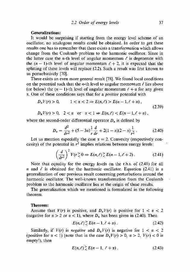
There exists an even more general result [78]. We found local conditionson the potential such that the rc-th level to angular momentum / lies above(or below) the (n — l)-th level of angular momentum / + a for any givena. One of these conditions says that for a positive potential with
DaV(r) > 0, 1 < a < 2 => E(nJ) > E(n - \J + a ) ,(2.39)
DaV(r)>0, 2 < a or a < 1 => E{nJ) < E(n- \J + a ) ,
where the second-order differential operator Da is defined by
Let us mention especially the case a = 2. Convexity (respectively con-cavity) of the potential in r2 implies relations between energy levels:
Note that equality for the energy levels on the r.h.s. of (2.41) for alln and t is obtained for the harmonic oscillator. Equation (2.41) is ageneralization of our previous result concerning perturbations around theharmonic oscillator. The well-known transformation from the Coulombproblem to the harmonic oscillator lies at the origin of these results.
The generalization which we mentioned is formulated in the followingtheorem.
Theorem:Assume that V(r) is positive, and DaV(r) is positive for 1 < a < 2
(negative for a > 2 or a < 1), where Da has been given in (2.40). Then
£ ( n , / ) > £ ( n - l , / + a ) . (2.42)
Similarly, if V(r) is negative and DaV(r) is negative for 1 < a < 2(positive for a < 1) (note that in the case DaF(r) > 0, a > 2, V(r) < 0 isempty!), then
E(n,f)<E(n-l9 / + a ) . (2.43)

38 Two-body problems
Proof:The main idea is to transform the Schrodinger equation in such a way
as to be able to apply the techniques explained previously: starting from(2.2) we make the change of variables from r to z and change of wavefunction from un/ to wn/:
z = r\ wn/(z) = r^un/(r), W(z) = V(r), (2.44)
which is a special case of a more general transformation [79] and gives
U(z;E) = Wif\ 7 f , (2.45)
where X = (2/ — a + l)/2a denotes the new angular momentum. Equation(2.45) can be considered as a Schrodinger equation with angular momen-tum A, potential U(z;E) and energy zero. From the assumed positivity ofE(nJ) and DaV(r) for 1 < a < 2 we deduce by straightforward computa-tion that AzU(z;E) > 0; therefore there exists a new potential U9 whichhas a zero-energy state of angular momentum A + 1 , and a wave functionwhich has one node less than wn/. Returning to the initial Schrodingerequation (2.2) one gets a state with angular momentum / + a and a poten-tial which is above the old one. The new potential now depends on n andE(nJ), but that does not matter. We deduce, again using the min-maxprinciple, that E(nJ) > E(n — 1,/ + a). The reversed sign for a > 2 ora < 1 follows from the assumption that DaV(r) < 0 for a > 2 or a < 1.
The proof of the second part of this theorem is similar. •
Examples:A source of examples is given by pure power potentials e(v)rv, where e
is the sign function. Then DxV(r) reduces to e(v)[v—2(a—l)][v+2—a]r v~2.In this way, we get
V = r4, E(n - \J + 2) < E{nJ) < E(n - \J + 3),V = r, E(n- l , / + 3/2) < E{nJ) < E{n~U + 2),V = -r"1/2, E(n - 1, £ + 1) < £(n, /) < £(n - \J + 3/2) l ]
V = -r"3/2, £(H - \J + 1/2) < £(n, /) < £(n - \J + 1).
Remark:We observe that there are potentials which solve the differential equation
DaV(r) = 0 and which are transformed into Coulomb potentials.

2.2 Order of energy levels 39
Theorem:The potentials
"~2 ~ a 2 Z r "~ 2 > a > 0, Z > 0, iV > ^ (2.47)
have zero-energy eigenvalues for angular momentum quantum numbers /which satisfy
A = 2 / ~ 2 a + 1 =N~n-1> w = 0,1,2,..., (2.48)
where n denotes the number of nodes of the corresponding eigenfunction.
Proof:With a change of variable from r to p = ra, the radial Schrodinger
equation with potential V^g, angular momentum { and energy zerois transformed into the Schrodinger equation for the Coulomb potential—Z/p, angular momentum X and energy —Z 2/4N2. It remains to remarkthat the Coulomb quantum number N need not be integer: the algebraictreatment of the Coulomb problem [67, 78] works for general real angularmomentum L •
Remark:One may also do a direct algebraic treatment for the potentials described
in theorem (2.47). Let us define
(2.49)
with Dirichlet boundary conditions at r = 0. One calculates easily, on theone hand, the product of A~ and A+:
w i t h
and, on the other hand, that the commutator is
/ ] a ; i V , z / + a - Ha>N>z/). (2.52)
This shows that
r ~ a # N Z / ^ = A^J2~ *H^NZ/ - (2.53)

40 Two-body problems
The ground-state wave function uo/ for H^N,Z/ is the solution of thedifferential equation A*ZJUOJ = 0 and is given explicitly by
uo/(r) = /+le~z^2N . (2.54)
Furthermore, proceeding inductively we see that
Un/-m = A~Z/_mUn-l/-(n-l)a (2.55)
is a solution ofHa,N,Z/-naUn/-na = 0 .
The case a = 2, which is a comparison to the level ordering for thethree-dimensional harmonic oscillator, is special.
Corollary:
If D2V(r)>0 then E(nJ) > E(n- \J + 2),if D2 V{r) < 0 then £(rc, /) < E(n - 1, t + 2). ( 1 5 6 )
Proof:Since D2 contains no zero-order term, the conditions D2V(r)^0 are
equivalent to A[/<0 when we make the same transformations as in theproof of the foregoing theorem. Therefore, both of the inequalities for thelevels of U yield the inequalities for the levels of V. m
Remark:One can define a 'running elastic force constant' K(r) by Vr(r) = K(r)r.
The conditions D2V(r) > (<)0 are then equivalent to the monotonicity ofK : Kf(r) > (<)0. This is analogous to the case a = 1, in which we canconsider a 'running Coulomb constant' Z(r) defined by V'(r) = Z(r)/r2.Then, AV(r) > (<)0 means Z'(r) > (<)0.
Remark:In Theorem (2.42) one may avoid the assumption that V is positive
and reformulate it in terms of U(z; E); but then the condition is energy-dependent. Eliminating the energy dependence in such a condition leadsto the next results.
Theorem:If the potential V(r) fulfils
(r^2 + (3 " 2 a) (jy) ) V ^ < 0 for a > 2 , (2.57)
we deduce that E(n, t) < E(n - 1, £ + a).

2.2 Order of energy levels 41
Proof:We start from the transformed Schrodinger equation (2.45) in the vari-
able z = ra and use a refined version of our previously derived theorem(2.42)-(2.43) [71]. There exists a solution to (2.45), with X increased byone unit and energy zero and a potential lower than U if
I(z) = AzU(z; £) < 0 wherever J(z) = i~U(z; E) > 0 . (2.58)dz
J(z) positive means explicitly that
--^{W{z)-E). (2.59)
Now it is simple to realize that (2.59) together with negativity of<0, (2.60)K(z) = z^(
dz \(ximplies that I(z) is negative for a > 2. Note that
azl(z) = az2/a~3K(z) + (2 - a)J(z). (2.61)
Condition (2.60) rewritten in the variable r gives (2.57). •
Remark:For pure power potentials we get nothing new compared to Theorem
(2.43), but condition (2.57) is — as it should be — invariant under achange of origin of energies.
Since we did not find a way to weaken the condition AU(z;E) > 0,removing the energy dependence in that case can be done only with thehelp of an additional assumption.
Theorem:Let V(r) be monotonously increasing dV/dr > 0, and assume
f r^-, + (3 - 2a)4-) V(r) > 0 with 1< a < 2 , (2.62)y drl dr)
then
E(nJ) > E(n - \J + a). (2.63)
Proof:This time we assume that K(z) is positive, which, rewritten in the
variable r, means (2.62). In order again to use (2.62) and to deduce thatI(z) is positive for a > 2, we would like to show the positivity of J(z). This

42 Two-body problems
can be obtained by noting that E{nJ) > W(0) from the monotonicity ofthe potential, and W(z) — W(0) can be bounded, since
W(z) - W(0) = — ^ — izW - f dy^\ (2.64)2(<x — l) L Jo y )
and K is positive. This shows thatW{z)-E(nJ) < —?—zW'(z) (2.65)
Z(0C — i)
and implies positivity of J(z) and I(z).Finally we formulate the result that follows.
Theorem:Assume that V(r) fulfils
then E(n, /) < £(n - 1, / + a).
+ (3 - a ) ^ < 0 for 1< a < 2 , (2.66)
Proo/:This time we observe that
2-
(2.67)Assume now that
( £ ^ ) (168)
dyW\y) = - ^ z ^ + / dy U ^
which is equivalent to (2.66); this shows that
E{nJ) - W(z) < -^—zW'(z). (2.69)2 — OL
Now splitting I(z) from (2.58) in an obvious way so as to eliminate theterm proportional to E(nJ)— W(z\ we deduce that AzU(z;E(n^)) isnegative by again using (2.68). •
Conjectures:Besides the expected result for the comparison with the order of energy
levels of the harmonic oscillator we have obtained a series of new andunexpected results, illustrated by the examples (2.47). However, whenone tests these inequalities numerically one sees that they are not asconstraining as one might expect. For instance, for the potential V = In r,which corresponds to v —• 0, we do not get anything new, but just

2.2 Order of energy levels 43
E(n - \J + 1) < E(nJ) < E(n - \J + 2). We may ask whether thefactors (3 - 2a) in conditions (2.57) and (2.62), as well as the factor(3 — a) in condition (2.66), are optimal or could be replaced by differentfactors. Based on the harmonic oscillator approximation for large angularmomenta and on numerical checks we are led to formulate improvedversions of Theorems (2.57) and (2.62)-(2.66) as conjectures.
Conjecture:Assume that V(r) fulfils
[ r-fo - (a2 - 3)4-1 V(r) < 0 for a > 2, a < 1 . (2.70)y dr2 dr J
We conjecture that E{nJ) < E(n — 1,/ + a). If, on the other hand,
Ir4^ - (a2 - 3)4- I V(r) < 0 for 1 < a < 2 , (2.71)y dr2 dr J
we conjecture the reverse ordering E(nJ) > E(n — \J + a).We have a number of arguments supporting this conjecture.
First argument:For smooth potentials and large / , we expect that the effective potential
- ^ + V(r) (2.72)
will, near its minimum, look more and more like an harmonic oscillator.With jy being the place of the minimum of Vf(r):
— = V'irt), (2.73)
we expect that for / going to infinity with n staying finite the energy levelswill be determined by the harmonic oscillator frequencies around jy:
E(n, t) ~ Vf(rs) + (2n + l )y j VJ^ > (2*74^
where the curvature is given by
(2.75)
Since one expects for smooth potentials that for / —> oo and r<? —> oo [60]
(2.76)

44 Two-body problems
the leading term in (2.74) will be given by V{. Substituting ( + A/ forinto (2.74) and using
- Vfa) ~ ijt+u - rdj/Ard = 0 , (2.77)
which holds at the minimum, gives for the energy difference
£(n, / + A/) - E(n, t) ~ * W v ) - *>(ry) ^ ( 2 / +2
1 ) A / . (2.78)
One may now ask for which value of A/, does £(n, /) equal E(n— 1, /+A/) .This will be the case if the r.h.s. of (2.78), which can be related to V\r^)by using (2.73), equals the contribution from changing n to n — 1 in (2.74).With the help of (2.75) we get
( 2 . 7 9 )
Therefore, we deduce the equality of the energy levels in the limit we areconsidering if
rtV"(r<)= [(A/)2 - 3] V'(r<). (2.80)
Furthermore, if the l.h.s. of (2.80) exceeds the r.h.s. one expects E{nJ) >E(n — \J + A/) and vice versa for large / . Since for smooth potentialsgoing to infinity for r —> oo, we expect the WKB approximation to bevalid for £ finite, n —• oo, we expect at least for confining potentials thatE(nJ) ^ E(n — \J + 2) [69] and only one of the inequalities will survivefor A/ > 2 or A/ < 2 for n - • oo, / finite. Thus we expect (2.70) and(2.71) to hold.
Second argument:For pure power potentials we found an asymptotic expansion of E(nJ)
in decreasing powers ofY + 1/2. First, we again approximate
by an harmonic oscillator and calculate anharmonic corrections. It turnsout that (for pure power potentials) the first-order perturbation due tothe term V}v(r^)(r — r/)4/4\ is of the same order as the second-orderperturbation due to V]ll(ji)(r—r^) 3/3!. It is tedious but simple to calculatematrix elements of x3 and x4 using the (a + eft) representation of x. (Asimilar expansion can be found in Ref. [80].) The final answer is

2.2 Order of energy levels 45
Table 5. Energy levels for the potential V(r) = r4 for the angular momentumand f + y/6.
n0 1
0
11+V6
22+V6
33+V6
44+V6
55+V6
3.812.67.1
16.910.821.414.926.119.331.123.936.3
11.622.816.027.720.632.825.538.130.543.635.749.3
21.234.026.439.531.645.237.051.042.656.948.363.0
32.146.237.852.243.658.349.564.555.570.961.977.3
44.059.250.165.656.472.162.778.769.285.675.792.2
56.772.963.379.769.986.676.793.583.5
100.690.4
107.7
70.387.377.294.484.2
101.691.2
108.998.4
116.2105.6123.7
84.5102.391.7
109.799.0
117.2106.4124.8113.9
E(nJ) ~ ( i|v2/(v+2)
From this expression one gets2/(v+2)
" 2 ) ( V + 1 } + -
This again supports the conjecture that
E(n, t + V2 + v) > E(n + \J) for v > 2 (or v < - 1 ) ,
but
E(nJ + V2Tv) < E(n + \J) for - 1 < v < 2 . (2.84)
Third argument:A numerical evaluation of energy levels — for example, for the potential
V(r) = r4 — gives the values for energy levels listed in Table 5. It is seenthat all values calculated for 0 < n < 7 and 0 < / < 5 support the

46 Two-body problems
conjecture that E{nJ) < E(n — 1,/ + y/6); no violation has been found.A similar test has been made for V = In r.
As is seen for 0 < n < 7 and 0 < t < 5, we find E(n-1, /+V6) > E(n, t).Furthermore, (E(n-J + >/6) - E(n,f))(E(n9f) - E{n - I,/))"1 does notexceed 15% for n < 6.
A more favourable case is V = r5. In this the effective potential
- ^ + r 5 (2.85)
has the property that, at V\r) = 0, one has also V"'(r) = 0. This makesit possible to squeeze V between convenient upper and lower bounds.Specifically, after a rescaling to
+25
we can prove the following chain of inequalities:
)2+21(p-l)435(p-l)2+21(p-l)4 < 4+2p 5 -7 < 35 (-p1 \n
— ^ 1 . (2.86)sin2(7rp/2)
The l.h.s. is a harmonic oscillator perturbed by a quartic term, for which,according to Loeffel, Martin, Simon and Wightman [81] diagonal Padeapproximants give a lower bound. Specifically, for the Hamiltonian
dz* ' 'one has a lower bound,
Eo> —^TT •
The r.h.s. of (2.86) is a soluble potential according to Fliigge's book onpractical quantum mechanics [82]: If
V = a2 ( ^ 1 + M^I) , (2.87)V sin ocx cosz ax /
the energy levels are given byE = a2[i + X + 2n\2. (2.88)
In this way one gets an explicit analytic upper bound on E(\J) and alower bound on £(0, / + ^7). For t = 20 we get
E(n = 0, / = 20 + yjl) > 175.08779E(n = 1, / = 20) < 175.07415 ,
which means that the inequality holds. A numerical calculation by Richardyields respectively 175.2 and 174.5, which means that the first bound isvery good [83].

2.2 Order of energy levels 47
Beyond / = 20 it is possible to prove the inequality analytically. For/ < 20, a numerical calculation is needed. This has been done, and forinstance,
/ E(n = 0, / = V7) = 15.31j E(n = 1, £ = 0) = 13.43 .
If one accepts that programs of numerical integration of the Schrodingerequation are sufficiently accurate, this constitutes a proof for n = 0, v = 5.
Fourth argument:A special case of the first part of our conjecture with n = 1 and t = 0
is included in the following theorem, where only monotonicity is required.
Theorem:For a monotonous potential, £(1,0) < £(0,6) holds — in fact we can
show that £(1,0) < £(0,2.5).
Proof:For a monotonous potential V we can take as an upper bound a
potential F(r), being a constant V(R) forr<R and infinite for r > R.This gives an upper bound on £(1,0) < 4n2/R2 + V(R) for all R. On theother hand, the ground-state energy for angular momentum ( is alwaysbounded from below by
£ 0 / > inf* \v(R) + ^ ^ ] • (2.89)
Taking t — 6 gives a chain of inequalities and proves the assertion.The improvement mentioned (replacing 6 by 2.5) needs a more refinedargument. •
Conclusion — applications
Again there are at least three important applications of our results. Ourfirst motivation came from quarkonium physics, but the results can alsobe applied to muonic atoms and to atomic physics, as we have notedalready in this section. In the first two cases, both conditions
AV(r)>0, D2V(r)<0, (2.90)
are satisfied. In quarkonium physics all proposed potentials fulfil condi-tions (2.90), as can be verified by explicit calculations. Let us also notethat the standard potential
V(r) = - ^ + kr, a(r)small r - -1/ ln r , (2.91)

48 Two-body problems
n=2, €=0
n=1,€=1
n=0, €=2
n=1, €=0
A7=0, €=1
n=0, €=0
Fig. 2.3. Ordering of levels for potentials fulfilling AV > 0 and D2F < 0.
with a running coupling constant modifying the Coulomb-like behaviourat short distances fulfils (2.90). For small r, AV > 0 is nothing but theantiscreening typical of QCD. In order to check (2.90) for the muoniccase we consider the charge density p generated by V: p = AV. Astraightforward calculation, using the 'running elastic force constant' K(r)and Newton's theorem
[drr2p(r), (2.92)Jo
yields
r20(D2V)(r0) = r0K'(r0) = p(ro)-(p)r<ro = ^ f ° drr2[p(r0)-p(r)] , (2.93)
r0 Jo
where we denote by (p)r<r0 the mean value of p(r) in the ball of radiusro. A decreasing charge density thus generates a potential with D2V < 0.
Thus for both quarkonium systems and muonic atoms (here we use theexperimental fact that for most nuclei the charge density is decreasingfrom the centre of the nucleus) the energy level ordering is between thatof the hydrogen atom and the harmonic oscillator, in the sense that (seeFigure 2.3)
E(n + I,/) > E(n,t + 1) > E(n + 1, f). (2.94)The third application to atomic physics was discussed in Section 1.1.
Let us note here in addition that for excited-state energy levels of the

2.2 Order of energy levels 49
neutral alkali-metal atoms Sternheimer [84] introduced a new orderingscheme. Motivated by measured energy level values he observed near-degeneracy of levels when n + 2/ is introduced as a new quantum number.This situation corresponds to a = 1/2. From Theorem (2.47) we observethat there exists a potential giving exact degeneracy for such levels at oneenergy.
Remark:The previous results were obtained for potentials which fulfilled condi-
tions like (2.39) where the second order differential operator Da, Eq. (2.40),appeared. It turns out that in two further problems, one concerning therelationship between moments [85] and the other constraints on the totaland kinetic energy of ground states [86], similar conditions will be used.For convenience, we define two classes of potentials:
Class A: For all r > 0, one of the following conditions holds
(i) DaF(r) > 0, 1 < a < 2, V(r) > 0 ,
(ii) DaV(r) > 0, a < 1, V(r) < 0 , (2.95)
(iii) f r2 —2 + (3 - 2a)— j V{r) > 0, l < a < 2 , - j ~ > 0 .
Class B: For all r > 0, one of the following conditions holds
(i) DaV{r) < 0, a > 2 or < 1, V(r) > 0 ,
(ii) DaV(r) < 0, 1 < a < 2, V(r) < 0 , (2.96)
(iii) ( r2—, + (3 - 2a)— ) V(r) < 0, a > 2 .y drl dr I
Splitting of Landau levels in non-constant magnetic fields
It has been recognized that the degeneracy of the so-called Landau levels,the levels of a charged particle confined to a plane subjected to a constantmagnetic field, play an essential role in the quantum Hall effect [87].We thought that it might be of some interest to use the 'technology'developed in the case of central potentials to study how the degeneracy isremoved when the magnetic field is not constant [88], and to consider, first,the simplest case — the one in which the magnetic field has cylindricalsymmetry around an axis perpendicular to the plane.

50 Two-body problems
So we consider the magnetic Schrodinger operator
in two space dimensions.Fixing the gauge, we suppose that A is of the form
(2.97)
(2.98)
Then the magnetic field B depends only on r and is given by
B(r) = dxAy- dy Ax = 2a(r) + r ^ - . (2.99)
Since the angular momentum is conserved, H^ splits into an infinite familyof radial operators which reads, in its reduced form,
rn2 — -A
In the case of a constant magnetic field, B (i.e., a = B/2 in our gauge),the energies are given by
E(n,m) = B(2n + l), (2.101)
where n denotes the number of nodes of the corresponding reduced radialwave function. Therefore, all energy levels are infinitely degenerate (in m).
For general B(r) the Schrodinger operator H^ may have rather sur-prising spectral properties. We illustrate this fact by an example given inRef. [89]: We take a(r) = fc(l + r)~y ,y > 0. Hence B{r) = 2fc(l + r)~^ -ky r(l + r)~y~{ and B(r) —> 0 as r —> oo. Therefore, the essential spectrumof H^ is equal to R j . There are the following three cases:
y < 1: Then the potential term in each Hm goes to infinity as r —• oo. SoHm and therefore H^ has a pure point spectrum (i.e., only eigenvalues).On the other hand, the spectrum equals RQ~. Therefore, the point spectrumis dense.
y = 1: Then the potential shifted by — k 2 is a long-range potentialgoing to zero as r tends to infinity. Hence Hm (and therefore H^) hasan (absolutely) continuous spectrum in (/c2,oo) and a dense, pure-pointspectrum in (0,/c2).
y > 1: In this case the potential term is a short-range potential, andtherefore there is only a continuous spectrum.
Our main results are the following:
Theorem:Let Emj^k) denote the eigenvalues of the two-dimensional magnetic
Schrodinger operator H^ corresponding to a magnetic field, orthogonal

2.2 Order of energy levels 51
to the plane, of strength B(r) = Bo + XB\(r),X > 0, where r is the two-dimensional distance.
Then we have, for all n > 0 and m > 0,
lim -. [Em+U(k) - EwW] > 0 if ^ <0 . (2.102)/—>o A Ur
Our second result holds beyond first-order perturbation theory, but onlyfor purely angular excitations.
Theorem:Consider the two-dimensional magnetic Schrodinger operator for the
field B(r). Suppose that the field B(r) is positive for large r. Then
From the physical point of view the ordering result is quite obvious.The distance of an eigenstate from the origin increases with the angular
momentum m. Thus, if the field B grows (or decreases respectively) withthe distance, the eigenstates feel a stronger (weaker) field and thereforethe energies should increase (decrease) as a function of m within a Landaulevel.
For the proof of Theorem (2.102) we shall use the supersymmetricstructure of the constant-field Schrodinger operator, i.e., Hm is factorizableand there are ladder operators acting between the Hms.
For Theorem (2.103) we use the supersymmetry of the operators H% —B(r) and a comparison theorem for the purely angular excitations of ¥L A.
Proof: Theorem (2.102)First of all, we present a suitable factorization of the reduced Hamilto-
nians Hm in the case of a constant magnetic field. We have
j2 m2 _ i
Hm = ~^ + ~7^ + a2°r2 ~ 2mao' (2'104)
where ao = Bo/2. Its spectrum is (4ao(n + l/2\neN°). We define the ladderoperator and its conjugate
d m+l , d m+iAm = —- + 2-+aor , *m = T + + a°r ' 1 1 0 5
dr r dr rWe have
= Hm + 4a0 (m + ^ , AmA+ = Hm+i + 4a0 (m + (2.106)

52 Two-body problems
and the intertwining relation
HmA+=A+Hm+1.
If we denote by un^ the reduced eigenfunctions we find
(2.107)
with c2nm = 4ao(n + m + 1).
From the ladder operators we deduce the following useful sum rules.Let W be a differentiable spherically symmetric function. Then, denotingby (.|.) the L2 inner product with respect to dr,
Cnm(Unsn\W\unjn+l) = (un,m\W \AmUn,m) = (A+Unfm+i\ W\un,m+l) (2.109)
and thereforeW (m +
aor)W
= ( «n, m aor) W (2.110)/
by
In the general case we write the radial part of the vector field as+ Xa(r). In the first-order approximation (in X) the energies are given
- ma(r)\un,m) (2.111)
Therefore, for the splitting we have
1
un,m+A (2.112)
Applying the sum rule with Wf = a(r) we find
\
-«n,m
aorz - m - - J a(r) - I ——*• + aor Un,m+1 }
(2.113)
- m - -
Again using the ladder operators we obtain
= Wm|C/|lVn+i) > (2.114)

2.2 Order of energy levels 53
where
Since
dr \ r2 J \ dr J
and
we have, after integrating by parts,
K%+1 = — jr^P- r (flo - ^ 4 ^ J un/n(s)unjn+i(s)ds dr . (2.118)cnm J Clr Jr \ S J
Now we can show that1 poo ( m + i \
F(r) = — / [ao j± unim(s)un^m+1(s)ds (2.119)cnm Jr \ S J
is strictly positive for r > 0. Using wn,m+i = (l/cnm)Amun^m we find usingintegration by parts
F(r) = Um(r) (ao - ^ ± 1 ^ + /°° (a20s - **=*) ulm{s)ds • (2.120)
On the other hand, multiplying the eigenvalue equation for un,m bywn?m and integrating from r to infinity we get
"• . / r \ ] ^ 4 f . 2 / r \ ^^2^.2 / x
~^.Un^rn ^2 W",mVr; — a0r un,m\r)
Us - ^ j u ^ d s . (2.121)
Hence
\ [ ( ) ( )(2.122)
Now F(0) = 0 and limr_+oo f(r) = 0. At critical points of F(r) we havethe following possibilities.
(i) Ifivm(r) = 0thenUn,m{r))2 > °5
h e n c e F(r) > °-

54 Two-body problems
(ii) If a0r2 = m + l /2 thenF(r) = ((d/dr)un,m(r))2 + ao(4m + 2)u2
n Jr) > 0.
(iii) If (d/dr)unjjr) = (aor + (m + l/2)/rK,m(r) thenF(r) = (An + 2)aou2
m(r) > 0.
Hence Theorem (2.102) is proved. •
Proof: Theorem (2.103)We study the one-parameter family of Hamiltonians
HA(X) = HA - XB(r), with B(r) > 0 for large r . (2.123)
For /I = 0 we have the operator describing the motion of a spinless particlein the magnetic field B(r), while for X = 1 the Hamiltonian #^(1) is theprojection onto the spin-down component of the Hamiltonian describingthe motion of a spin-1/2 particle in the field B(r). This Hamiltonian,however, has an infinitely degenerate ground state of energy E = 0 [89].
In fact, considering the family of reduced Hamiltonians
Hm(X) = Hm(0) - XB(r) (2.124)
withj2 m2 _ i
Hm(0) = - - p + — ^ + ct(r)r 2 - 2ma(r) (2.125)
and denoting the nodeless, reduced eigenfunctions by um(X), i.e.,
Hm{X)um{X) = Em{X)um{X), (2.126)
we have Em(l) = 0 for all m > 0 and
um(lr) = cmrm+12 exp (- J'sa(s)ds) . (2.127)
By the Feynman-Hellmann theorem the derivative of Em(X) with respectto X equals the expectation value of the magnetic field, so that we find forthe splitting of two eigenvalues
-^ [Em+1(X)-Em(X)] = (um(X)\B\uM)) ~ (um+1(X)\B\um+1(X))
(2.128)JO \ar /
with
I(r,X) = f \u2m+1(X,s) - u2
m(X,s)] ds . (2.129)Jo

2.2 Order of energy levels 55
We have to consider the cases dB/dr > 0 and dB/dr < 0 separately.
dB/dr > 0We want to show I{r,X) < 0. To do so we analyse the Wronskian of
and um
w(r) = wm(A, r)—u m+i(k9 r) - um+i(k, r)—u m(k9 r) ; (2.130)ar ar
w(r) vanishes both at zero and at infinity and
^w( r ) = f i w ( V ) H m ^ ^ . (2.131)
If we denote the square bracket by h(r) we have
( 2 , 3 2 )
For fields J5(r), finite at the origin (less singular than a two-dimensionaldelta-function is also sufficient), r3(da(r)/dr) equals zero at the origin.Since
the square bracket is a strictly decreasing function and therefore thepositivity of w(r) implies that um+i(A9r)/um(k9r) is strictly increasing. SinceJ(r,/l) vanishes at zero and at infinity we have I(r,l) < 0. Hence:
^ 0 . (2.134)
Integrating from 0 to 1 with respect to A we find
£m+1(0) - EM(0) > £w +i( l ) - Em(l) = 0 • (2.135)
dB/dr < 0We prove the ordering result by contradiction. Again we analyse the
Wronskian w(r) of um+i and um. We write its derivative as follows usingB(r) = 2a(r) + r(da(r)/dr)
d_ um{X,r)um+i{X,r)dr r2
x [2m + 1 - B(r) -r2 + r 3 ^ + r2 ((EM) ~ Em+iW)] . (2.136)
Denoting the square bracket by k(r) we have
dk(r)dr = 2r(Em(A)-Em+l(X)-B(r)). (2.137)

56 Two-body problems
Now we prove the result by contradiction. For this we note that /(r, 1) < 0,as can easily be checked. Hence:
j - [Em+i(k) - Em{X)} U=1> 0 . (2.138)aA
Thus, either £m+i(/l) < Em(A) for all Ae[0,1), or there is a first point2* (starting from 1) such that Em+i(V) = Em(A*). But then dk(r)/dr =—2rB(r) < 0 since B(r) is non-negative by assumption.
As before, we conclude that I(r,A*) < 0. Hence:
j - Em(X)] U ^ > 0 , (2.139)aA
which yields the desired contradiction.
Remark:Our proof does not work for excited states, since the lemma does not
hold for states which have nodes.Generalizations of the above results to Hamiltonians with an additional
scalar potential have been worked out by one of us (H. G.) and Stubbe[88].
2.3 Spacing of energy levels
We turn now to the problem of the spacing of the energy levels, and, firstof all, to the spacing between the angular excitations — i.e., the stateswith n = 0 (zero node) and £ arbitrary. For this we need first to presentthe remarkable discovery of Common [90] concerning the moments of thewave functions of these angular excitations:
poo(rv)t= / u2
0/(rVdr, (2.140)J 0
which follows from lemma (2.28). This says that for a given sign of theLaplacian of the potential the reduced wave function divided by / + 1
is logarithmically concave (AF > 0) or convex (AV < 0). We shall notfollow the original derivation of Common [90], which used integration byparts, and instead shall present the following somewhat stronger result,obtained by Common, Martin and Stubbe [91].
Theorem:If the potential has a positive (negative) Laplacian outside the origin,
the quantity

23 Spacing of energy levels 57
where the numerator is the expectation value of rv in the ground state ofangular momentum / , is respectively logarithmically concave or convex— i.e., log(M/(v)) is concave or convex. Before giving the proof, let usindicate that in Common's original result the moments jumped by oneunit. For instance,
(r-^^oir)^ < ^l(l)/=o|2 (2.142)
for AV > 0.Another important remark is that Common's original inequalities, as
well as the more general ones, lead to inequalities of the type of theSchwarz inequalities for AV < 0, while they give inequalities going in theopposite direction, such as the example given above, for AV > 0.
Now we start with the proof. First of all we shall use the function
which is logarithmically concave (convex) if the Laplacian of the potentialis negative (positive) for all r > 0. Then the problem is to study thelogarithmic concavity of
= f^Y} J <t>(N(v) = f^Y} J <t>(r)rvdr . (2.144)
For this purpose we consider the quantity
N(v) - 2xN(v +e) + x2N(v + 2e)
rv+e rv+2e.2 rv
r(v + l) T(v + l+e) F(v + l+2e)dr. (2.145)
The square bracket in Eq. (2.145) has two zeros in R+ because itis a second degree polynomial in xr6 with a positive discriminant as aconsequence of the logarithmic convexity of the gamma-functions. Let0 < y\ < yi be the two solutions of the equation
-r—\ / . A \ T"1/ i l l \ ' "I""1/ i 1 i ^ \ ? ^ i l iv^
then the square bracket in (2.145) vanishes at

58 Two-body problems
Now we construct the expression
rv 2xrv+e x2rv+l€
= J[<l>(r)-Ae-Br] dr9
(2.148)where A and B are adjusted in such a way that the first square bracketvanishes at r\ and r2. Because of the logarithmic convexity or concavity of4>, this is always possible, and the first square bracket has no other zero.Hence we get
/ x \ 2N(v) — 2xN(v +e) + x2N(v +2e) — An - ) < 0 (2.149)
if AF>0 .The simplest case is AF < 0. Then, from (2.149) and from the positivity
of A it follows that for any x
N(v) - 2xN(v +e) + x2N(v + 2e) > 0 ,
and this implies
(N(v + e))2 < N(v)N(v + 2e),
which demonstrates the logarithmic convexity of Af, and hence of M/(v).For AF > 0, one must find x and B such that x = Be. Then, the
combination of JVs in (2.149) is negative for some x, and this implies thatits discriminant is positive. But this can be done only by a fixed pointargument that we now sketch. The key point is that we have to impose4>{ri)/4>{n) = exp(-B(r2 - n)) with R = r2/n = (y2/yi)1/e, yi and y2being given uniquely by Eq. (2.146). Furthermore, x = B€ = y\/r\.
Hence, we have to show the existence of a solution of (j)(Rr\)/4>{r\) =exp(—y { (R— 1)); the l.h.s. goes to unity for r\ —> 0 and to —oo for r\ —• oobecause of the logarithmic concavity of <\>. There is therefore a solutionand the second part of the theorem is proved.
We leave it as an exercise for the reader to generalize these results tomixed moments , i.e., Juo/ uo/'rvdr.
It remains to generalize these results to the case where, instead of havinga Laplacian of a given sign, the potential belongs to one of the sets Aand B previously introduced in Eqs. (2.95) and (2.96), which are obtainedby a change of variables. We shall limit ourselves here to the special case,where (d/dr)(l/r)(dV/dr) has a given sign, i.e., where F is concave orconvex as a function of r2. Then all one has to do is to change variablesz = r2, and the theorem becomes:

2.3 Spacing of energy levels 59
Theorem:If V is convex (concave) in r 2
log r , +°2t + 3)/2) i s c o n c a v e (convex) in v . (2.150)
Now, we have all that we need to study the spacing of energy levels.There are, of course, other consequences of Common's result — forinstance, inequalities on the kinetic energy and the wave function — butthese will be considered later.
The first problem we attack is the study of the concavity or convexityof £(/), the energy of the ground state, characterized by n = 0 and / , as afunction of (. For a harmonic oscillator potential we know that £(/) is alinear function of/. For a general potential we know first of all that £(/)is increasing because by the Feynman-Hellmann theorem
dE Z*00 u 2
-(n = (2,+ l)jo -£*. ,2.151)and we also know that it increases more slowly than t{t + 1), since,according to a general theorem indicated in Section 2.1, the energy ofthe ground state is a concave function of any parameter entering linearlyin the Hamiltonian. For an infinite square well £(/) indeed behaves liket(f + 1) for large L
We return now to the comparison with the harmonic oscillator. Firstwe consider the case of a potential concave in r2 — i.e., such that(d/dr)(l/r)(dV/dr) < 0. Naturally, the angular momentum can be takenas a continuous variable, and we have to prove that the quantity
is positive for arbitrary 3 to establish that the energy is a concave functionof / . An upper bound on E{t — b) and E(t + 6) can easily be obtainedby using the trial functions r~su^(r) and r+su^(r), respectively (notice thatthese trial functions become exact in the harmonic oscillator case).
Elementary algebraic manipulations, using the Schrodinger equation forM/, lead to
(2.152)\u2r-2~2bdr fu2r-2+2Sdr
( 2 / + 1 - 2S)JV2 2 < ; - ( 2 / + 1 + 2 8 ) J U r " r
Ju2r-2SdrV2 2 < ; - ( 2 / + 1 + 2 8 ) r 2Ju2r-2Sdr Ju2r2Sdr
From the concavity of log (rv)/F((2/ + 3 + v)/2), it is easy to see that ther.h.s. of (2.152) is positive. Therefore, we have

60 Two-body problems
Theorem:If (d/dr)(l/r)(dV/dr) < 0 for all r > 0, £(/) is concave in t.Its converse is also true, but the demonstration is 'trickier', and is given
in Appendix B. At any rate, we have obtained [48] the theorem:
(2.153)
The borderline case is naturally the harmonic oscillator for which £ is alinear function of f.
Subsequently, the analogue theorem has been obtained for the case ofpotentials with a Laplacian of a given sign [50]:
Theorem:If
\ (2.154)3 dE
Although we do not want to give the proofs of these two theorems inthe text let us indicate the essence of the proofs. In both cases extensiveuse is made of the Chebyshev inequality:
If / and g are both decreasing or both non-increasing and h is non-negative :
f fhdx I ghdx < f fghdx I hdx . (2.155)
For (2.153) one uses
> 0 (2.156)\ru/ r~
and for (2.154)
> 0 . (2.157)r2
A weaker, but more transparent, version of the second theorem isobtained by integration. That is,
<~Erc(2.155)

2.3 Spacing of energy levels 61
if AF(r)<0 Vr > 0, and where Ej designates the Coulomb energy. Thenthe r.h.s. of (2.158) is
0 / _i_ 1 / f \ 2(2.159)
In the introduction, we have given illustrations of this inequality, withmuonic atoms — for which AV(r) > 0 — and alkaline atoms, for which,in the one-electron approximation, one has AV(r) < 0.
Until now we have ignored spin effects, but the technology developedso far makes it possible to take them into account, in the case of spin 1/2particles, in a semirelativistic treatment (a la PaulV. Then it is known thatthe splitting between the states J = ( + 1/2 and J = t — 1/2 is, to firstorder in an expansion of the energies in (v/c)2, given by
where the expectation value is to be taken between Schrodinger wavefunctions of given orbital angular momentum and where V is the centralpotential entering the corresponding Dirac operator as a vector-like quan-tity. We shall designate d(^) the splitting corresponding to a purely angularexcitation (i.e., with a nodeless radial wave function).
Then, we have two theorems [50]:
^ + 3 ) 2 W + 1) E(S)] , (2.161)
for AF(r)>0 Vr > 0, and
' < / , , m > (2.162)
for AV(r)>0 Vr > 0.For their proof, the Chebyshev inequality previously mentioned in
Eq. (2.155) is essential, but we shall simply refer the reader to the originalreference. The most beautiful illustration of these inequalities is givenby muonic atoms (see Table 6). For small Z, A(^) the upper bound al-most coincides with the experimental value because the nucleus is almostpoint-like, while, for large Z — Lead, for instance — A/S exceeds 2.
Another area where similar interesting inequalities can be obtained isthat of the fine structure of the P states of quarkonium, which consist ofa triplet and a singlet. This structure is completely analogous to the finestructure of positronium. Strangely enough the singlet P state of the ccsystem has been observed and its mass accurately measured before thesinglet P state of positronium [92].

62 Two-body problems
Table 6. Fine splittings of levels of muonic atoms (S), their upper bounds (A)and their ratios.
Element
56pe
NatNjNatCu
68Zn
75As
89 y
93Nb
92Mo
114Cd
115In
120Sn
Z
26
2829
30
33
39
41
42
48
49
50
5(1)keV
4.20+0.09
5.306.17
7.00+0.611.10
+0.819.26
±0.9423.15
+125.50+0.839.90
+0.843.60+0.845.70+0.9
A(l)keV
4.40
5.896.78
+0.67.84
11.45
22.70
29.10
29.60
52.50
56.80
60.60
5(2)keV
0.47+0.07
1.68
0.56+0.65
2.00+0.8
2.27±0.8
2.68±0.22
2.7±0.4
5.16±0.5
5.35±0.96
5.65+0.9
A(2)keV
±0.7
2.74
5.07
5.98
5(3)keV
2.27±1.8
2.20±0.8
0.95+0.6
5(2)/5(l)> 0.0988
0.112±0.02
0.26±0.13
0.08±0.012
0.18±0.08
0.188±0.04
0.116±0.01
0.106±0.015
0.129±0.015
0.123±0.02
0.123+0.02
5(3)/5(2)> 0.211
1.00±0.8
0.43+0.2
0.43±0.2
There are four P states in a qq system (where q is a quark, or an electron),three triplet P states with total angular momenta J = 0, 1, 2 and onesinglet P state. In the framework of the Breit-Fermi approximation [93],which may or may not be correct, and assuming that the central potentialis made of scalar-like and vector-like parts
V = VS + VV, (2.163)
one finds
where2mz \r dr /
(2.164)
M = - ^ [-5M(13P2) + 27M(l3Pi) - 1O(13PO)] (2.165)
(notice that M is NOT the centre of gravity of the triplet P states).

23 Spacing of energy levels 63
One could, of course, use our previous result (2.161) to get a lowerbound on M(l1Pi), since we believe that the quark-antiquark potentialhas a positive Laplacian. But this turns out not to be terribly constraining.We prefer to use the information that V is concave, to get
(2.166)
Here again, the Chebyshev inequality is used in the proof. For the converseinequalities
' — \ < ? [ £ ( ! ) - £ ( 0 ) ] 2 (2.167)r I " 2
we only need V" < (V'/r)9 but an extra tool is the mixed sum rule alreadymentioned at the end of Section 2.1:
rooZ*00 dV 1 0 f/ UlUQdr= m)-E(0)]2
Jo dr 2 JoThe final conclusion for the case of charmonium when one puts numbersis, for mc = 1.5 GeV,
3536.2 + 12.2 MeV < M ( l 1 P i ) < 3558.6 + 12.2 MeV ,
where the error is a crude estimate of relativistic effects. This is in agree-ment with the observation of a *Pi state, six months after this predictionin Ref. [94] M = 3.526 GeV.
For the Upsilon system, we predict
9900.3 + 2.8 MeV < M ^ P i ) < 9908 + 2.8 MeV .
We now turn to the spacing of radial excitations — i.e., excitationswhere the angular momentum is fixed and the number of nodes increases.A number of results have been obtained by Richard, Taxil and one ofthe authors (A.M.) [49]. As we shall see, these results are interesting butincomplete and some conjectures still need a completely rigorous proof.Again, the harmonic oscillator will be our starting point. Indeed the / = 0levels of the three-dimensional harmonic oscillator are equally spaced:
2E(n, £ = 0) = E(n + 1, / = 0) + E(n - 1, t = 0) .
When we (Richard, Taxil and A.M.) undertook this study we hopedthat the same criterion as before, i.e., the sign of (d/dr)(l/r)(dV/dr) woulddecide whether the levels get either closer and closer with increasingn or more and more spaced. This is not true. We have examples ofperturbations of r2 /4 such that (d/dr)(l/r)(dV/dr) > 0 for which, forsome ft,

64 Two-body problems
while we expected the opposite. In pure power potentials, V = rv, thenaive expectation seems true, i.e.,
2E(n, 0) > E(n + 1,0) + E(n - 1,0) for v > 2 .
What we have proved was completely unexpected, although a posterioriit was understood. It is as follows:
Theorem:For
_r2
X being sufficiently small, the levels get more and more spaced withincreasing n, if
lim r3v = 0r->0
and
Z(r) = j-r5^--^- > 0 Vr > 0 . (2.168)dr dr r dr
If, on the other hand, Z < 0, the levels get closer and closer as n increases.However, this is not always true outside the perturbation regime, as weshall see.
Now, why do we need the condition (2.168)? Z is a third-order differ-ential operator in v. There are two obvious vs which make Z equal tozero. These are
v = const, v = r2 .
However, Z = 0 admits another solution, i.e.
1v = -~ ,rl
and this is perfectly normal. Adding v = C/r2 to the harmonic oscillatorpotential is equivalent to shifting the angular momentum by a fixedamount, and since the Regge trajectories of the oscillator are linear andparallel — i.e., (d/d/)(£(n,/)) is constant, independent of n — all levelsare shifted by the same amount and equal spacing is preserved. Naturally,we could invent other criteria, since knowledge of all f = 0 levels does notfix the potential — as all experts on the inverse problem know. There is aninfinite-dimensional family of potentials with equal spacing of t — 0 levels,the parameters being the wave functions at the origin, but we believe thatwe have here the simplest criterion.

2.3 Spacing of energy levels 65
The proof again uses the technique of raising and lowering operators.We want to calculate
1A = SEN+I + <5£JV-I
where EN = E{NJ = 0). If V = r2/4 + Av, then
A = / " v[u2N+1 + u2
N_{ - 2u2N]dr ; (2.169)
UJV-I and MJV+I are obtained from UN by using raising or lowering opera-tors:
/ r2 d\ ,2JV + 2 - — + r— )u N = y/(2N + 2)(2N + 3)uN+l
\ 2 dr)(2.170)
/ r2 d\2JV + 3 - - - r - j M j v + i -
Then, one performs a series of integrations by parts with the purpose oftransforming A into an expression containing explicitly Z(r) denned in(2.168), taking into account the boundary condition lim,--^ vP = 0. Onegets
r , (2.171)JO \ar ar r ar j
where
/
oo A-uf poo pa
% / W /r /5 Jr' Jr"the explicit expression of K(r) is
2N{2N + 1){2N + 2)(2N + 3)K(r) =
2 [ 3£ 3 E2 Er
+ uN =• 1
UpjUN — —^ + ^~2 * (2 .1 /2)
It is possible (but painful) to prove that (2.172) is everywhere positive.Then Theorem (2.168) follows.
Unfortunately this theorem only holds for perturbations, as severalcounterexamples show. The best counterexample is obtained by takingone of the partly soluble potentials obtained by Singh, Biswas and Datta[95] and much later by Turbiner [96] of the form V = r6 - (2K + l)r2.

66 Two-body problems
For K = 4, the energies of the first five levels are given by
Eo, E4 = +V480 + 96VTT
It is clear that the spacing is not increasing in spite of the fact thatZ, calculated from V is positive. However, no counterexample has beenfound for Z positive and V monotonous increasing.
It may be some time before this conjecture is proved. In the meantime,we shall try to obtain another criterion, based on the WKB approximation.For a monotonous potential, E can be considered to be a continuousfunction of N, defined by
N - i - i (2.173)
(Here the ground state is given by N = 1, not N — 0!) Then the spacingis given by dE/dN, and levels get closer with increasing N if
d fdE> - (2.174)
(2.175)
(2.176)
dN \dNi.e., exchanging function and variable:
1E2>
We have, differentiating under the integral sign,dN 1 fr' drdE
where rt is the turning point. We cannot differentiate again, because wewould get a divergence at rt. So we assume V'(r) > 0, Vr > 0, and integrate(2.176) by parts
dN _ 1 r 1 F'dr _ 1lE~2HJ V\lE~^V~n' V'(0)
Henced2N 1
2^"1 V"
d£2 2TT F ' tO^E - F(0) 2TT JO
A sufficient condition for this to be positive is
V" < 0 ;
-.dr.
(2.178)

2.4 The wave function at the origin, the kinetic energy, etc. 67
however, notice that d2N/dE2 does not vanish for V" —> 0, since the firstterm survives and cannot be zero because V\0) is not infinite. In fact, fora purely linear potential, it is easy to prove rigorously that the spacingbetween the energy levels decreases.
We are convinced that Condition (2.178) is sufficient to ensure that theenergy level spacing decreases, but it may be some time before a rigorousproof is given.
In QCD, the quark-antiquark potential is believed to be concave [46].In this way we understand that in the case of the Upsilon (bb boundstates) and Charmonium (cc bound states) we have:
My" — My' < My' ~ My ,My'" — My" < My" ~ My' ,Mw» — Mw' < My,' — Mw .
However, the last observed level of the bb system, called yIV, is suchthat
MylV — My'" > My'" — My" .
We therefore have an indication that the naive one-channel potentialmodel breaks down. However, this level is high above the BB threshold
Myiv ~ 10.85 GeV > 10.55 GeV
and coupled channel effects or glue contributions or both may be impor-tant.
2.4 The wave function at the origin, the kinetic energy, mean squareradius etc.
Apart from the energy of the levels, other important quantities are themoments of the wave function, already introduced in Section 2.3 for thenodeless states, the square of the radial wave function at the origin, or,in the case of £ ^ 0, of its /-th derivative, the expectation value of thekinetic energy and the mean square radius of the state. Also of interestare matrix elements between states, such as electric dipole matrix elementsetc.
The wave function at the origin plays a role in the decay of positroniumor quarkonium. For quarkonium the so-called Van Royen-Weisskopf [97]formula (also proposed by Pietschmann and Thirring, and others) gives
Fe+e- = 1 6 ^ * , (2.179)
where eg denotes the charge of the quarks in units of e, and M the totalmass of the decaying state. For the decays of the P states of quarkonium,

68 Two-body problems
into photons or gluons, analogous formulae exist involving the derivativesof the wave function (see, for instance, Ref. [97]).
The expectation value of the kinetic energy plays a role, for instance,in the mass dependence of a quark-antiquark system for a flavour-independent potential, because of the Feynman-Hellmann theorem:
J-E(m) = - ^ , (2.180)dm m
where E is the binding energy of the quark-antiquark system and m isthe common mass of the two quarks. A trivial change has to be madefor unequal masses. The kinetic energy is also related trivially to the totalenergy for pure power potentials, but there are more general inequalitieslinking the two for a given sign of the Laplacian if V tends to zero atinfinity, and also consequences for the dependence of the spacing of thecorresponding levels on the mass.
The importance of the mean square radius is obvious, because it is ameasure of the size of the system, and it is desirable to relate it to moreaccessible quantities like energies.
All these quantities, as we shall see, are linked together by all sorts ofinequalities, some of which are rather tight and can be of physical interest.
Returning to the wave function at the origin or its derivative let usremark first that it is, in fact, the limiting case of a moment:
3 + v) v
In the special case of n = 0, this will allow us to use the arsenal oftheorems obtained at the beginning of Section 2.3, but for the time beingwe shall look specifically at radial excitations, with mostly / = 0. A firstresult follows [98]:
">0 V r > 0 |<o(O)|2$Ko(O)|2 . (2.182)
Theorem:If
Proof:uio(r) has at most one node. By looking at the Wronskian of uo$(r)
and uio(r) it is easy to see that (wo,o(r))2 — (ui,o(r))2 vanishes at least once(because of the normalization) and at most twice. From the Schwingerformula, written for 2m = 1,
(u'(0))2 = / u2(r)--dr , (2.183)Jo ar

2.4 The wave function at the origin, the kinetic energy, etc. 69
we see that it is impossible to have (u[0(0))2 = (uf00(0))2 if V" is either
constantly positive or constantly negative, because then (uiyo(r))2—(wo,o(?0) 2
would vanish only once, at r = ro, and we would haverco r -, rj Ay "I
0 = /o [Ko(r))2 - (uo,o(r))2] [ -F( r ) - —(r o)J dr . (2.184)If F" is negative we cannot have (u[0(0))2 > (UQO(O))2 because we havethe opposite inequality for a Coulomb potential and, in the continuousfamily of concave potentials,
one potential would give a zero difference of the wave functions at theorigin. For the case V" > 0 a similar argument can be used by taking
It is tempting to make the conjecture [99]
l<o(O)l<K+i,o(O)l for F " < 0 , VFI, (2.185)but this conjecture, so far, has resisted all attempts at proof. In the limitingcase V(r) = cr, we have |t/w>0(0)| = |u'n+1>0(0)| V n , according to (2.183). Allwe can do is to look at the limiting case V = r + Av, A small, V with agiven concavity. Then, by a mixture of numerical calculations for small nand use of the asymptotic properties of the Airy functions for large n, wecould 'prove' that
a M « ; » if ,•>„.Nevertheless a weaker, but solid result can be obtained:
Theorem:If
F " < 0 , F'(r)-+0, and V(r) -> oo,for r - • oo , K,o(°)l2 -* ° f o r n -* °° • (2.186)
Proof:If V" < 0, F is necessarily monotonous-increasing, because it cannot
have a maximum for finite r without going to —oo for r —> oo. Then thequantity uf(r)2 + (E — V)u 2(r) is monotonous-decreasing, as one can seeby calculating its derivative. Hence
> \u\r)\2 Vr > 0 ,

70 Two-body problems
and, by integration,
but, also,
\u{r)\2 < r2|t/(0)|2 ,2|t/(
\u(r)\2 < k(0)|2
E - V(r)Hence we get, by inserting both inequalities in (2.183):
1 + 2 / lrV(r)dr-RlV{Ri) In E(n,0)-V(R2)E(n,0)-V{Ri)
dV_dr
where 0 < Ri < R2 < RT, and where Rj is the turning point
E(n,0) = V(RT).We can choose R\ sufficiently small, but fixed, such that
(2.187)
l + 2/Klr|F(r)|dr-.R?7(Ri)Jo
is strictly positive. Then we can choose R2 such that &Vl&r{R.2) < e, earbitrarily small, and finally since V(r) -> 00, E(n,0) —> 00 for n —> 00, andwe can make the logarithm in (2.187) arbitrarily small. Therefore, for nbig enough, we can make |i/n0(0)|2 arbitrarily small, under the acceptableextra condition that J^r\V(r)\dr converges.
In the case of a potential going to zero at infinity but having an infinitenumber of bound states, we also have the property |t^0(0)|2 —• 0 forn —> 00. Let us impose the condition
^ < 0, with V(r) -> 0 as r - • 00 , (2.188)
which guarantees that the potential decreases more slowly than r~2+€ andhas an infinite number of bound states accumulating at zero energy.
We write, using obvious inequalities,
K,o(O)l2 -f' rdr
-dr dV 2
and hence, if R is small enough,
l<o(O)|2 -JR[l- / 0* r2{dV/dr)dr\ '
where (T)n is the average kinetic energy. But, from (2.188)
X1 In <- I^V^?UJI s

2A The wave function at the origin, the kinetic energy, etc. 71
and because E(n,O) goes to zero for n —• oo, the desired result follows.Conversely if V" > 0, V > 0, V -» oo for r -> oo, we have K ?0(°)l2 - •
oo for n -> oo. The proof is simple because V cannot be singular at theorigin. One gets
|<o(O)l2 > ^rrR dr
Jo E(n,0)-dV(R)
dr Jo E(n,O)-V(r)
One can take R sufficiently large to make dV(R)/dr arbitrarily large, andthen n big enough to make the denominator arbitrarily close to unity. •
A final indication in favour of our conjectures is the WKB approxima-tion. Averaging for large n over the oscillations of the square of the WKBwave function, i.e., replacing
sin2 [J ^E ~ v{r')dr\ x const" (£ -
by
one gets, after some manipulations,
VV" / V\~1/2
^ ( ) • ( 2 - 1 8 9 )
which means that |M'(0)| decreases when E increases for V" < 0, and thereverse for V" > 0. This is a continuous version of our conjecture.
Another approach to the wave function at the origin has been proposedby Glaser [100]. He starts from the matrix element
(x\e-Ht\y) , (2.190)
which for x = y reduces to
(x\e-Ht\x) = J2\xPn(x)\2e-E» t, (2.191)
assuming that the potential is confining and that, hence, we have a purelydiscrete spectrum. The simplest result is: if the potential is positive,
(x\e-Ht\x) < (x\e'Hot\x) , (2.192)
which implies, in three dimensions,
V-i i M2 ! eENt
X><*)l < (4

72 Two-body problems
and, minimizing with respect to t,
k=l6n
(2.193)
which has the same qualitative behaviour as the semiclassical estimatethat we shall soon derive.
Now we no longer assume that V is positive, but only that / \V-\yd3xconverges, with y < 3/2, F_ being the negative part of the potential. Thenwe can prove that [100]
(x\e~Ht\y)- 1
or
lim
0 for t -> 0 ,
= 1.k=i
Then, thanks to a Tauberian theorem of Karamata, we can prove that
f=1 \Wk(x)\2 Jlim
73/2 6 T T 2 '(2.194)
which agrees exactly with the semiclassical result obtained by Quigg andRosner [59] — at least for non-singular central potentials in the WKBapproximation:
(2.195)
Our result (2.194) has the advantage of being valid for any confiningpotential less singular than — r~2+e at the origin. For instance, for V = In rit gives
N
\ipk(0)\2 ~ const x (IniV)3/2 .k=\
In fact, our approach applies to any x, without spherical symmetry, andwith mild extra assumptions one can prove
Li\Vk(x)\2-([EN-V\lim
iV-+oo E0 , (2.196)
N
which means that if one fills a confining potential with N independentparticles one gets, for large N9 the Thomas-Fermi density.
Now we wish to derive inequalities on the expectation values of thekinetic energy as a function of energy differences. Initially this was done

2.4 The wave function at the origin, the kinetic energy, etc. 73
by Bertlmann and one of the present authors (A.M.) [101] using sumsover intermediate states by a technique somewhat similar to the oneused to derive the Thomas-Reiche-Kuhn and Wigner sum rules [97]. Butour inequalities hold, in fact, even for non-integer angular momentum,using Regge's analytic continuation. To prove them one must use theSchrodinger differential equation directly. First, we derive an inequalityon the mean square radius:
)<|~. (2.197)
All we need is an upper bound on £(0,/ + 1), which can be obtained bytaking the variational trial function
uO/+i = Cruoj , (2.198)where uo/ is the exact wave function of the state (0, /). The calculation isstraightforward and gives (2.197). It is not a surprise that (2.197) becomesan equality if V(r) is a harmonic oscillator potential, because then thetrial wave function given by (2.198) becomes exact.
Now we have a kind of Heisenberg uncertainty inequality:4(T)0 / ( r 2)0 />(2^ + 3)2. (2.199)
This inequality can by proved by expanding the quadratic form given by
dr>0 (2.200)
and writing that its discriminant is negative. Combining (2.197) and (2.200)we get
2/4-1(T)o/ > - j - [E(0y + 1) - £(0,/)] . (2.201)
This inequality is completely general and becomes an equality if V is aharmonic oscillator potential. It will be used at the end of this section tocalculate the mass difference between the b-quark and the c-quark fromexperimental data.
If one adds extra conditions one can get inequalities in the oppositedirection. For instance, if
d_i_d_v<0dr r dr
(T)o/ < — J - [£(0, t) - £(0, t - 1)] . (2.202)
The proof of this inequality will be given after we have discussed the'Common' inequalities [90] between the expectation value of the kineticenergy and that of r~2, which we shall now proceed to present.

74 Two-body problems
Consider first the case where the Laplacian of the potential has a givensign. Then the radial kinetic energy in the state u — UQ/ can be written as
From Lemma (2.28), we get
ju'2dr>^J^+l)dr (2.203)if
AF>0.Combining with the centrifugal term we get
( 7 V % (/ + 1) (V + i ) (r-2)0/ (2.204)
ifAF>0 V r > 0 .
A similar treatment can be given for all cases A and B given inSection 2.2 resulting in
(T)o/ %(f + ^ ) it + 1/2) <r-2)0/ (2.205)
if V belongs respectively to sets A, a or B, a.A special case is a = 2, corresponding to a given sign of (d/dr)(l/r)
(dV/dr),
if
Combining this inequality for the case in which
dr r drwith the concavity of £(0,/) — see Theorem (2.154) — we get
(T)o/ < (t + £) ~ < [E{W - E(0^ - 1)] ,which is precisely (2.202).
Let us notice that although we have so far proved these inequalitiesonly for the ground state for a given (, they hold, in fact, in one direction

2.4 The wave function at the origin, the kinetic energy, etc. 75
for arbitrary radial excitations. One has for arbitrary n
(TV > (/ + W + l/2)(r-2)n/ (2.207)
for AV > 0, and
( T V ^ ( ' + 3 /2)( / + l/2)(r-2)M / (2.208)
for
However, these inequalities are never saturated for n > 1. Their proof isvery simple. Consider a state with n nodes. Consider the interval betweentwo successive nodes rk < r < rk+i, and take as a potential
— 1 for r < rk
= V for rk<r <rk+1 (2.209)
N- l forr > rk+i .
If F satisfies, for instance, AF > 0, then F/c^+i also satisfies AVkji+i > 0for N > 1 and hence taking the limit N —> oo we see that inequality (2.207)holds for the ground state of this limit potential — i.e., for potential Vwith Dirichlet boundary conditions at r^ and r^+i. Hence
u'n/ "I 2— Mw/ \ dr > (/ + l /2)(/ + 1) / r un^dr
Adding up all such inequalities for all successive intervals gives (2.206).The same method allows one to prove (2.208). Notice that the oppositeinequalities are not valid for arbitrary n, because the construction (2.209)is impossible.
Now, since — as we have seen — the wave function at the origin isthe limiting case of a moment, we can obtain inequalities connecting thewave function at the origin and the expectation value of the kinetic energy[91, 102].
We have seen in Section (2.3) that
(rv)o/logr((v+2/
is concave (convex) if V belongs to class (A9 a) or (5, a), respectively. Onthe other hand we have
-3 r((v + 2 / + 3)/<x)

76 Two-body problems
Applying the convexity considerations to v = —2/ —3, v = —2, and v = 0,and using inequality (2.205), one gets
2 F ( (2 /+ 3) /«) / + 1 / 2 / ( T ) o /
(2.211)fqr classes ( 4, a) and (B,a), respectively, defined by (2.95) and (2.96).Interesting particular cases are, for / = 0,
K j & 2 (2.212)if AF>0, and
K0(0)|2 $ ^ (^)3 / 2 (T)$ =* 1-2284(7)^ (2.213)
if
d_l_dV>0.dr r dr K
An interesting example is V = r, corresponding to class .4 with a = 3/2which gives
which is not too far from the exact answer (3/£o)3//2 — 1.455.These results can be applied to quarkonium physics. The kinetic energy
satisfies the Bertlmann-Martin inequality (2.201) which for n = 0 , / = 0reduces to
(T)o,o > \ [E(n = 0J = l)-E(n = 0^ = 0)] . (2.214)
Noticing that the quarkonium potential is concave and increasing, we seethat (2.213) applies and in this way we get
1 f M 13//2
M0)|2 > -^ [-J-W = 1) - W = 0)]J . (2.215)If we substitute this inequality into the Van Royen-Weisskopf formula(2.179) we get, with
M(n = 0 , / = l) = 3.52GeV,M(n = 0 , / = 0) = 3.10GeV,
Fe+e- > 3.9-5.2 keV with a c-quark mass between 1.5 and 1.8 GeV. This

2 A The wave function at the origin, the kinetic energy, etc. 11
is to be compared with
Te+e- = 4.7 + 0.35 keV
obtained experimentally. This is almost too good, but we must rememberthat the Van Royen-Weisskopf formula needs some substantial correc-tions.
Similarly, for the bb system, one gets, with
M(n = 0 y = 1) = 9.90 GeV,Af(w = 0 y = 0) = 9.46 GeV,
and a quark mass of 5.174 GeV
Te+e- > 0.7 keV ,
compared to the experimental value of
Te+e- ~ 1.34 + 0.05 keV.
Now we shall use the previous inequalities on the kinetic energy tostudy the mass dependence of the binding energy and also the energylevel separation.
Expression (2.181) gives the derivative of the binding energy with respectto the common mass of a system made of a particle and an antiparticlebound by a mass-independent potential (in the case of quarkonium a'flavour-independent' potential). Following Ref. [101] we have
E(m) - E(M) = f ^-dfi. (2.216)Jm /I
Now remember that if we consider the Schrodinger equation
d2 „, ,lidr2 u = 0 , (2.217)
enters linearly in the Hamiltonian, and according to a general the-orem — see the remark after (2.10) — the ground-state energy of theHamiltonian is concave with respect to this parameter, i.e.,
d dE
Using (2.180) we get
—(/IT(JU)) > 0 , (2.218)d\x
so that from (2.217) we obtain
E(m) - E(M) > mT(m) \- - -U for M > m .|_m M \

78 Two-body problems
Then adding the quantum numbers which had previously been omitted,and using inequality (2.201), we get
E(m,n = 0,<f = 0) - E(M,n = 0 , / = 0) >
3 M - m yE{fnn = O y = i) _ E(m,n = 0 , / = 0)].4 MNow we use
MQQ(H, / ) = 2me + E(mQ9 n91), (2.219)
where mg denotes the quark mass and MQQ the total mass of the quark-antiquark system, to get
Ml(» = <U = 0)-Ma(,, = <U = 0)
With nib = 5 GeV this gives us m\) — mc> 3.29 GeV, while the inequalitym\) — mc> \{Mhi — MCc) gives rnb — mc > 3.18 GeV.
This is as far as we can go without imposing any restriction on thepotential. We have seen in Section 2.1 that by scaling for power potentialsV = ra /a, one gets from the Schrodinger equation
V \iarL \irL I
E(n) ~ /n~^+i and T(n) ~ fT^+i .
In this way we see that in the particular cases of a Coulomb potential(a = — 1), or linear potential (a = 1), T(/i) behaves like \i or like \i~1^respectively.
The 'good potentials' for quarkonium are, as we have seen in theintroduction, such that
^> . »d^< » . (2.221)dr dr dr2
These are particular cases of restrictions of the type
XV' + rV"^ Vr>0 , (2.222)
the vanishing of (2.222) corresponding to a power potential with X = 1—a.From (2.222) we see that
(X -l)(v+ l-rV^j + ^ ( 3 - X) (2.223)
is increasing or decreasing respectively. Consider now the Schrodingerequations for two masses, m and M, M > m. Combining them and

2.4 The wave function at the origin, the kinetic energy, etc. 79
integrating we getu'(M,r) tu(M,r) u(m,r) u(M,r)u(m,r)
If V is monotonous-increasing, and if u(M9 r) and u(m, r) are ground-statewave functions, we see that u(M,r)/u(m,r) is decreasing and takes thevalue 1 only once at r = ro. If we now take the expectation values of(2.223) for M and m, take the difference and use the virial theorem, weget
(X - l)(E(M) - E(m)) + (3 - X)(T(M) - T(m))
= I [(X - 1)7 + rV - [{X - 1)V + rV'}r=ro] [u2(M,r) - u2(m,r)] dr .
Under condition (2.222) we get, respectively,
(1 - 1)(£(M) - E{m)) + (3 - X){T{M) - T{m)) < 0
or, going to the differential form,
(1 _ ylM + (3 _ x)** < o (2.225)
and integrating, we get T(ix)pil~x^~x decreasing (increasing).In particular, if the potential has a positive Laplacian and is concave,
which is condition (2.221) and which corresponds to X = 2 and X = 0, weget
( T(fi)/fi decreasesI (2.226)[ T()u)iu1/3 increases .
Obviously, (2.226) gives a stronger restriction than (2.220). One obtains
E(m,n = 0 , / = 0) - E(M,n = 0 , / = 0)
9 f / m \ 1/31> 4 rKMj [E(m9n = 09S=l)-E(m9n = 09* = 0)] ;
when this is applied to the quarkonium system one gets
mb-mc>- [Mbh(n = 0 , / = 0) - Mc-C(n = 0 , / = 0)]
/ m \ i / 3 \
WJ ) [Mc~c{n = °y = 1} " Mc'c(n = ° ^ = °) ] *With nib = 5 GeV this gives
mb-mc> 3.32 GeV , (2.227)

80 Two-body problems
which is a substantial improvement. If one wants to go further one mustabandon rigour, and replace inequality (2.201) for / = 0 by a realisticguess. In Ref. [101] such a guess was made. It was
(2.228)with c = [£(1,0) + £(0,0) - 2£(0,1)] / [£(1,0) - £(0,0)] J
This expression has been manufactured in such a way that the bound(2.201) is always satisfied and is saturated for a harmonic oscillator poten-tial, for which c vanishes. It also fits a pure Coulomb potential. Numericalexperiments with the potential — A/r + Br and with pure power potentialsgive agreement to a few parts per mille.
T(nib) and T(mc) can then be estimated:
T(mc) ~ 0.346 GeV ,
T(mb)~0Al GeV.
Taking the average T in the integration, one gets, for m^ = 5 GeV and5.2 GeV,
mb-mc~ 3.39 and 3.38 GeV , (2.229)
respectively. The sensitivity to mb is therefore very weak. For anotherapproach involving leptonic width see Ref. [102].
We turn now to another mass dependence, that of the spacing of energylevels [103]. For power potentials this is trivial by scaling [59]. The spacingbetween two levels with given quantum numbers behaves like ^-a/(a+2)for V = ra/a. For the separation between the lowest levels, (1,0) and(0,0), (0,1) and (0,0) and, more generally, between two purely angularexcitations, we can impose a condition of the type (2.222). It is easy tosee that the wave functions WO,L and UQ/ of two purely angular excitationsintersect only once, and that WO,L < ^0/ for small r. Thus, assuming (2.222)and taking the difference of two expectation values of (2.223) in the states(0,L) and (0,*f), we get
{X - l)[£Gu,0,L) - £(/i,0,/)] + (3 - A)[T(/i,0,L) - 7>,0,/)] > 0
if
AV + rV"%0
and hence

2A The wave function at the origin, the kinetic energy, etc. 81
i.e.,
AE x /i 3=1 decreasing (increasing).
In particular, if
AV > 0 (k = 2), (2.230)
A£/i decreases ;
if
V" < 0 (A = 0) , (2.231)
increases, as would be expected.One can also apply these considerations to the 2S-1S separation if the
wave functions intersect only once. This is the case for (2.231). But if weonly require AV > 0 the wave functions may intersect twice. So we obtainthe following:
Theorem:If AV > 0 and V" < 0,
-0-0» decreases and
[£(//, 1,0) - E(fi, 0,0)] fii/3 increases with \i. (2.232)
It will not be a surprise to the reader to learn that these properties arewell satisfied by the charmonium and upsilon systems, with
£(mc, 1,0) - £(mc,0,0) = 3686 - 3097 MeV = 589 MeV
and
E(mb, 1,0) - E(mb,0,0) = 10023 - 9460 MeV = 563 MeV .
To end this section, we would like to discuss mixed moments — i.e.,matrix elements of the type
poo/ un/rvunl/'dr.
JoFirst of all, Theorem (2.141) can be adapted trivially. If we call
a r(/ + e* + v + 3)'then, if wo/ and t*o/' are ground-state wave functions with angular mo-menta / and / ' and if the potential has a positive (negative) Lapla-cian, lnM^'(v) is concave (convex) in v. The analogous theorem, if

82 Two-body problems
(d/dr)(l/r)(dV/dr) has a given sign, also holds: if
d_ld_Vdrr dr<
N,,(v)=
is logarithmically concave (convex).The theorem can be used to obtain upper and lower bounds on electric
dipole matrix elements [104]. Upper bounds are rather trivial:
\j uO/(r)uO/+i(r)rdr\ < j (uo/(r))2r2dr ,
using Schwarz inequality and the normalization of U0/+1. Then, using(2.197), we get
]'^;'^<'. (2.233)Obtaining a lower bound is trickier. First of all we have the sum rule
f00 2f + 3 Z*0 0
/ —9—uojuoj+idr = (£(0, / + 1) - £(0, /)) / uo/uo/+idr ,Jo ^ Jo
obtained by calculating the Wronskian of wo/ and wo/+i- Then we assume(d/dr)(l/r)(dV/dr) < 0, and employ the logarithmic convexity of N//+i(v) forv = —2, 0, and 1, making use of the previous identity. Hence we get
•2 [/ u0/u0/+idr]22W + 5/2)2 / r ( / + 2)/ uo/uO/+irdr
It only remains now to get a lower bound on f uo/uo/+\dr, in terms ofphysically observable quantities. The trick of Common [104] is to takewo/ — ^MO/+1J with X = [/Mo/Moz+idr]"1, as trial function for the firstradial excitation. In this way one gets a lower bound on £(1,/) which,after some algebraic manipulations gives
r f/ u0/u0/+1dr
2 £(1, {) - £(0, t + 1) + 2(/ + 1) / d
At this point, there are various possibilities:
(i) keep only the assumption (d/dr)(l/r)(dV/dr) < 0, then

2.4 The wave function at the origin, the kinetic energy, etc. 83
which gives
\ f I 2
/ uO/uo/+1rdr\ >
X
2)£(1, t) - £(0, t + 1) + ((2/ + 2)/(2/ + 3))[£(0, { + 2) - £(0, ^ + 1)]
[£(0, / + 1) - £(0, /)] [£(1, /) - £(0, /)]
(ii) add the assumption AV > 0. This will guarantee that the lowerbound is non-trivial because £(1,0 > £(0,/ + 1). But one can dobetter by integrating (2.154). One then gets
and hence
[£(0, / + 1) - £(0, /)] [£(1, /) - £(0, /)]
For the Upsilon system one finds in this way
1.76 GeV~1/2 < (r)0,i < 2.61 GeV"1/2 .
This is not too bad, considering that several of the inequalities used arenot optimal.
Up to now, we have considered electric dipole transition momentsbetween states with zero nodes — i.e., with positive radial wave functions.Transition matrix elements between states with n ^ 0 in the initial or thefinal states might vanish. However, there are a few results that one canobtain for matrix elements
Kf = J UnAr)ur>Ar)rdr , (2.234)
where \t -1'\ = 1, and n + nr < 2.Here we shall not give the details of the proofs which are given in
Ref. [105], but only indicate the basic ingredients:
(i) uo/r(r)/uo/(r) is increasing for / ' > t\
(ii) (ruoj/uoj+i) increases (decreases) if V'/r increases (decreases);

84 Two-body problems
(iii) the sum rule (already used is this section)
(En/ - Erff) / Un/Un'/rdr = / -2Un
where \i is the reduced mass of the particles;
(iv) the sum rule (already quoted in Section 2.1)
= / —Un
(v) the fact that if
(v) = Jrvp(r)dr,the number of zeros of /(v) is less than or equal to the number ofzeros of p(r).
The results, in a simplified form, are the following:
(1) £>oV+i cannot vanish, and if we decide that the wave functions arepositive near the origin, it is negative.
(2) £>o/+1< ° i f (l/r)(dV/dr) is increasing (decreasing),1 /'-U1
Do/ = 0 for an harmonic oscillator potential.
V = f e(a)p(a)ra£i.7-3/2-3/2
or iff2
V = p(a)rada
with
e(a) = sign of a
p(a) > 0 .
Conversely there exists a value of a,
—1 < a < + 1 ,
such thatvo/+\ - u

2.5 Relativistic generalizations of results on level ordering 85
for
V = e(a)ra .
(4) DjJ+1 + 0 for
= / e(oc)p(ayda .
This is perhaps the most interesting non-trivial property since existingpotential models for quarkonium belong to this class.
2.5 Relativistic generalizations of results on level ordering
In the previous sections we have obtained a number of results on levelordering of energy eigenvalues belonging to different quantum numbers ofn and /, where n denotes the number of nodes of the radial wave functionand t the orbital angular momentum, as well as inequalities for pureangular excitations of the Schrodinger equation. A question we are oftenasked is: What happens if relativistic effects are taken into account? Wehave already discussed the splitting of multiplets if relativistic correctionsare treated in first-order perturbation theory. The next cases to treat arethose of the Klein-Gordon and Dirac equations. First of all, it is clearthat not all inequalities can be generalized. For some, which becomeequalities in the case of pure Coulomb potentials in the Schrodingerequation, this is no longer the case if one uses the Klein-Gordon or theDirac equation. In addition, for the Dirac equation with a vector-likepotential, the energy levels depend on the main quantum number AT, thetotal angular momentum J and fe, where \k\ = J + (1/2), or, equivalently,on / the orbital angular momentum. It has been shown by one of theauthors (H.G.) [57] that the degeneracy in k for the Coulomb potential islifted in such a way that
E(N, J, -k) > E(N9 J,k), if AV % 0 V r > 0, fc > 0 (2.235)
after perturbation by a potential V.For example, this means that, in spectroscopic notation, the Nsi/2 level
is above the Npi/2 level if AF > 0 for all r > 0. However, this result isestablished only in the first order of perturbation theory and there is noinequality connecting energy levels with the same N but different Js. Forthe pure Coulomb case we know that for fixed N, the energies increase asJ increases.
There is a result, obtained by Palladino and Leal-Ferreira, for the specialcase of an equal mixture of scalar and vector potentials [106], but this

86 Two-body problems
does not tell us what happens in the neighbourhood of a pure Coulombpotential which is vector-like.
We shall first discuss the results for the Klein-Gordon equation
[p2 + (m + S)2 -(E- V)2]xp = 0 (2.236)
and afterwards turn to the Dirac case. For the pure Coulomb case S = 0,V = —(Za)/r, with Za < 1/2, we know the solution explicitly, since theterm V2 in (2.236) can be incorporated in the centrifugal term in thereduced radial equation
/ d2 i / ' ( / ' + !) t 2 2 Z a \
--r-^ H = Ym -E -IE—)u = 0, (2.237)y dr2 r2 r Jwith
/ 1 \ 2 / 1 \ 2 o
- ( Z a ) 2 . (2.238)
Hence, (2.237) looks like a Schrodinger equation with a Coulomb poten-tial, and we get energy levels
E(n, t) = (2.239)
\Here E denotes the total energy. From (2.239) we see that for fixedN = n + S + 19E increases as t increases.
Before stating results on level ordering, we note that the energy levelscan still be labelled by n and t and the trivial ordering properties
E(n + 1, /) > £(n, t) and E(n9 L) > E{n91) for L > t (2.240)
hold. They are indeed satisfied provided that V < 0 and E(n9t) > 0.Then the coefficient of u, the reduced wave function, in the Klein-Gordonequation is a monotonous function of £, and this suffices to show the firstinequality of (2.240). The second follows from the Feynman-Hellmanntheorem applied to dE/d£ and the positivity of (E — V).
In the following we shall take S = 0 in Eq. (2.236), however, as will beremarked later, some results also hold for S > 0.
Theorem:If AV(r) < 0, V(r) < 0 and V(r) -* 0 for r -> oo and limr_>0 r V(r) >
—1/2, we obtain the strict inequalities
E(n9 /) < E(n - 1, t + 1). (2.241)

2.5 Relativistic generalizations of results on level ordering 87
We show this by regarding the Klein-Gordon equation as a Schrodingerequation dependent on a parameter E:
dr2 M = 0 . (2.242)
Under the assumptions made (we restrict ourselves to positive energystates), the Laplacian of the effective potential 2VE — V2 is negativebecause
\AV2 = 2 IVAV + (2.243)
Now, since AV < 0 and V < 0, rV has a negative limit for r -» 0, meaningthat the effective potential has a —1/r 2 singularity. Our general result ofRef. [56] can be extended to potentials such that limr_>o r2V(r) > —1/4 andcan therefore be applied. On the other hand, the non-linear dependence of(2.242) on the energy can be overcome by using a fixed point argument.
The weakness of this result is that there is no counterpart for AV > 0.To circumvent this difficulty we follow a procedure analogous to that usedin (2.237)-(2.239), i.e., we transfer a part of the potential into the angularmomentum term. We define, in analogy to the Coulomb case,
-Za= lim rV(r) (2.244)
and keep the definition of t' (2.238). Then the Klein-Gordon operatorbecomes
,2,45)
with
Next it can be shown that:
Lemma:IfAF>0Vr>0, V(r) < 0, lmv
AF>0 andV(r) = -Za, thenV2 > (Zaf/r2. (2.246)
After the change of variables E(n,f) = E{nJ) we may formulate thefollowing two-sided theorem:
Theorem:If AV > 0, V < 0, Hindoo r V(r) = -Za >-\-{,
E(n, /') > E(n -k,f + k). (2.247)

88 Two-body problems
Remark:When AV < 0, a prerequisite of this theorem is that the Klein-Gordon
equation make sense — i.e., that lim r_>o r V(r) > —\—£.It is straightforward to translate this result into the variable £
with
if + l-f - (Zap + k = y(£ + A + 1)2 - (Zap . (2.248)
In general, A will not be an integer if k is one. We have 0 < A(/, k) < kand in that sense (2.241) is a consequence of (2.247). Indeed, for AV < 0,etc., we have
E(n, £)<E(n-k,£ + A(£9 k)) < E(n - k, £ + k), (2.249)
because of the monotonicity of the energies with respect to the angularmomentum, which still holds for the Klein-Gordon equation for negativepotentials since
d£We note that in many situations A(/,fc) is very close to k.
If Za < 1/2 (which is required for £ = 0) we have fc —1/2 <c A(£ 9k) < k;if Za < 1, £ > 1, we have k - 0.4 < A(/,fc) < fc.
Using these remarks we can transform (2.247) into a result connectingonly physical angular momenta. If AV > 0, V < 0, limr_>oo F(r)r > —1/2,
£(n, / ) > E(w - fe, / + fc + 1). (2.251)
This is somewhat crude and does not reduce to the correct limit if Vbecomes a pure Coulomb potential. However, we can do better by provinga relativistic analogue of the result obtained by Martin and Stubbe [50]:
Theorem:If AV < 0, V(r) < 0, lim^oo r V(r) = -Za > - \ - t x ,
( m2
If AF > 0, 7(r) < 0 ,

2.5 Relativistic generalizations of results on level ordering 89
The proofs involve a chain of inequalities: the virial theorem for theinitial Klein-Gordon equation and a modified one combined with the factthat V < 0 and AF has a given sign:
E(E-(V))%m2 for AF < 0,(2.253)
< 7 V > -E(V) f o rAF<0 ,
where (f)n/r is the expectation value of -(d2/dr2) + (t\{' + l)/r2). Inaddition, the Feynman-Hellmann relation for £ as a function of / ' ,
2(£ - F) ^ ^ = (2/' + 1) ( ^ ) , (2-254)
and an inequality connecting the total kinetic energy and the angularkinetic energy established in the Schrodinger case by Common
(T)nJ' > K' + ~ ) W + 1) ( "2 ) for &V > °> e tc- >V 2/ \r /n/>( , 1\ , / 1 \
(T)o/' < / + - ( / + 1) ( -r ) for AF < 0, etc. (2.255)V 2 / Wo/'
have been used. The last inequalities imply an asymmetry since the lastone holds only for n = 0 if AF < 0. The first one holds for any n, but isoptimal in the Coulomb case only for n = 0.
Now we can combine (2.247) and (2.252) with A = /+A(^,/c), *f2 = ^+/cand obtain inequalities, involving only physical angular momenta whichreduce to the normal one in the non-relativistic limit, which give for thecase k = 1, for a potential with a positive Laplacian,
_x\ f m2
(2.256)For a negative Laplacian we have the opposite inequality, but it holdsonly for n = 1. And then, in any case, we have (2.241).
One may wonder about the field of application of these results. Itis tempting to apply them to pionic atoms. Unfortunately in this case,however, and contrary to the case of muonic atoms, the major distortionis not due to the size of the nucleus, but to strong interactions, includingabsorption by the nucleus. Quarkonium has also been described by Kangand Schnitzer [107] with the help of the Klein-Gordon equation, but apure vector confining interaction led to metastable energy levels.
Probably the most interesting conclusion is that we have found a casein which the obstacles in going from a non-relativistic situation to arelativistic situation are not insurmountable.

90 Two-body problems
We next turn to the Dirac case in which we have results, which are validin first-order perturbation theory about a vector-like Coulomb interaction[57] and a partial non-perturbative result about the order of levels withina multiplet [108].
For the Dirac operator the Coulomb potential again plays a specialrole. Although the spin-orbit coupling leads to the fine structure splitting,a certain two-fold degeneracy between levels remains. Our result concernsthe splitting of this degeneracy.
The standard treatment of the Dirac-Coulomb problem is rather in-volved. Therefore a treatment using the symmetry responsible for thedegeneracy is more appropriate. We note that in our previous proofsconcerning non-relativistic spectra we used supersymmetry in an essentialway. In addition, the ladder operators entering the factorization of theSchrodinger-Coulomb Hamiltonian are related to the Runge-Lenz vector.There exists a generalization of this vector for the relativistic situation. Inaddition, there exists a supersymmetric factorization which is very suitablefor studying the level splitting.
We now start to review briefly the algebraic factorization method whichallows us to obtain the spectrum and eigenfunctions of the relativisticCoulomb Hamiltonian
Here c is taken as unity y = Ze2,a are the Pauli matrices and 1 is the 2 x 2unit matrix. H acts on four-component spinors with wave functions whichare square integrable over R3. We need the normalized wave functionsand a mapping between eigenfunctions belonging to degenerate levels.
Rewriting (2.257) in radial coordinates gives a 2 x 2 matrix operator
_y _d k\r dr r
d k y
which acts on two-component wave functions; k = + l , + 2 , . . . where\k\ = J + 1/2 denotes the eigenvalue of the operator —o • L — 1, whichcommutes with H. There exists a simple transformation [109] from (Gk9Fk)to (Gk,Fk),
which allows (2.258) to be rewritten in a supersymmetric factorized way.

2.5 Relativistic generalizations of results on level ordering 91
We introduce first-order differential operators
4 = ±4- + - - -> P = Ekr, (2.260)dp p sk
where the index k has been suppressed. Gk and Fk fulfil the relations
A+Gk = (- + £) Fk , AoFk =(^-Tf)Gk. (2.261)
The discrete spectrum of H consists of a unique ground state for k =— 1 , - 2 , - 3 , . . . and a sequence of two-fold degenerate levels for k = +1,+2,^... For jiegative k the ground states are obtained from the conditionsA^Fk = 0, Gk = 0. This leads to
Fk = p*e-™'\ E(0,k) = , k = - 1 , - 2 , . . . .
/7
(2.262)No normalizable solutions for AQAQ exist at this energy. However, all theother eigenstates of AQAQ and ^Q^CT o c c u r i n pairs. They can be obtainedby the factorization method [109], since there are identities of the form
-A+A
A ± + V n e N _dp p Sk + n
The n-th eigenfunctions can be obtained from the solutions ofA'in = 0, Xn = p» +*£TW/<*+»> (2.264)
by forming Fk = AQ . ..A^Xn and evaluating Gk from Eq. (2.261). Gk andFk are then obtained by inverting (2.259). They correspond to eigenvalues
+ n)2
which are doubly degenerate for n > 1.In the following we fix n > 1 and \k\ and denote G ^ and F±^\ by
G± and F+, respectively. Similarly, we denote G+^i and F+^i by G+ andF. Note that F+^| does not depend on the sign of k. Our result may bequoted as follows:

92 Two-body problems
Theorem:The Hamiltonian H = a • p + fim — y/r + XV(r) has a discrete spectrum
E(n,k, A), labelled by fe = +1, +2,..., which is the eigenvalue of — {a L +1)and is related to the total spin quantum number J by \k\ = J + 1/2 andlabelled by n = 0,1,2,..., which counts states with fixed k and is relatedto the number of nodes of the radial wave functions. For n > 1, we haveE(n,fc, 0) - E(n, -fc, 0) = 0 and
^ ^ ^ ^ ^ ^ ^ O i f A ( r ) > 0 V ^ 0 . (2.266)
To prove this we have to determine the sign of
AE =(G+\VG+) + (F+\VF+) <G_|FG_)
(2.267)
where (.|.) denotes the scalar product in L2(R+,dr).Two steps remain. Firstly, we have to evaluate the normalization inte-
grals entering (2.267), and secondly, we have to find a mapping relating(G+,F+) to (G_,F_). With the help of a recursion relation the first task issolved with [57]
(F±\F±) + (G±\G±) = m ^ 1= ^(F\F) skE2
k (k + su)(k/sk + m/Ek) '
The second, more important, step consists in obtaining ladder operatorsmapping from states with one sign of k to states with the opposite sign.By explicit calculation we find that the operator A& intertwines betweenhk and h-k, where
/ d k my ydr r k r
\ r dr r k /
and h-kAk = Akhk. From relation (2.258) we obtain
(2.269)
/G_\ A /G+\ lk + sk k= ockAk I p ) , cck = \ 7 r n , ,—T^TT • (2.270)
\F-) \F+J y k-sk skEk(k/sk + m/Ek)This mapping allows simplification of the expression for A£.
Taking a few simple steps like partial integration and using the factthat for a pure Coulomb-like perturbation A£ has to vanish, we arrive atan expression which has a definite sign if the Laplacian of the potentialhas a definite sign.

2.5 Relativistic generalizations of results on level ordering 93
Remarks:If we assume the validity of the Hartree approximation in the relativistic
framework, we can expect from this result the splittings
2P1 / 2>2S1 / 2, 3P1/2>3S1/2, 3D3/2>3P3/2, etc. (2.271)
for alkaline atoms and their isoelectronic sequences. This is because theouter electron should move in a potential created by a point-like nucleusand the electron cloud of the closed inner shells, which has a negativeLaplacian.
The reverse situation occurs in muonic atoms, where at the most naivelevel the muon is submitted to the extended charge distribution of thenucleus, thought to be made of indissociable protons and neutrons. Henceby Gauss's law the Laplacian of the potential is positive. Also, the Lambshift may be viewed as coming from an effective potential with a positiveLaplacian, giving the splitting 2Pi/2 < 2Si/2. Unlike the Schrodinger casethis result still awaits a generalization beyond perturbation theory.
Our next result is that in the atomic case: if AV < 0, and if the potentialis purely attractive — i.e., — (y/r) + XV(r) < 0 — one has the completeordering of levels for fixed principal quantum number N, at least forperturbations around the Coulomb potential. That is, in spectroscopicnotation, we have
2P3/2 > 2P1/2 > 2S1/2(2.272)
3D5/2 > 3D3/2 > 3P3/2 > 3P1/2 > 3S1/2
etc.The new results are the first inequality in the first line, and the first
and the third of the second chain of inequalities, which, as we shall show,are generally true if the potential —(y/r) + XV(r) is purely attractive andmonotonously increasing (in our case the latter condition is guaranteed bythe hypotheses AV < 0). The other inequalities are taken from Ref. [57].We shall this time label the eigenvalues by the principal quantum numberN = 1,2,..., the total angular momentum J = 1/2, 3/2, ... and thequantum number k = +1, +2, .... In the general case the inequality weshall prove is the following:
ENJ=L-l/2,\k\ < £iV,J=L+l/2,-|/c|-l > (2.273)
which means that for fixed N and L the energy increases as the totalangular momentum J increases.
It was shown in Ref. [50] that in the expansion of Dirac eigenvalues toorder l/c2 the inequality (2.273) is always satisfied if AV < 0, even if thepotential is not purely attractive, since the splitting equals the following

94 Two-body problems
expectation value for Schrodinger wave functions:
(2.274)
This expression can be shown to have a definite sign, if AV < 0, by usingthe sum rule
y m^^UL + m =0r2 dr r3 / NJj
The eigenvalue problem for the Hamiltonian obtained from (2.256) byadding a general potential V to the Coulomb part may be reduced by astandard procedure [110] to a system of two coupled ordinary differentialequations,
(2.276)
r , ZG = ENJ,kF^
where ' denotes d/dr and EN,J,K denotes the positive eigenvalue.
Theorem:We impose the following conditions on the potential W = —(y/r) + XV
in Eq. (2.276):
C l : W is purely attractive, i.e., W < 0;
C2: W is strictly monotonous in r, i.e., Wr > 0;
C3: limr_>o r7(r) = 0 and y < 1.
T h e n £ J V 5 J i/ci ^ £jy,j+i,—iki—i*
The last condition means that (without loss of generality) the Coulombsingularity appears only in —y/r,y < 1, and guarantees the existence ofCoulomb eigenvalues. Since W < 0, we may obtain a single second-orderdifferential equation for G:
-W)2G + m2G
G = 0(2.277)
T 1 5 7 G + 4 G+m-W r2
k W+ m-W
Doing this for any pair k — \k\ > 0 and — \k\ — 1 we observe that theorbital-angular-momentum-like term is the same.
First of all we show that the monotonicity of W implies that
(2.278)

2.5 Relativistic generalizations of results on level ordering 95
In fact, suppose that
The idea is to construct a suitable eigenvalue problem depending on acertain parameter r\ which 'interpolates' between these two states. Thebasic trick is that, in view of the assumption that the energies are thesame, we may take Ex,j,k as a constant in certain places in Eq. (2.277).In addition, the coefficient of the 1/r2 term, k(k + 1), remains invariantunder the transformation \k\ -> — \k\ — 1. We shall replace Eq. (2.277) bya linear eigenvalue equation which depends on a continuous parameter Y\.If we label the corresponding eigenfunctions Gn,r\ = \k\ and r\ = —\k\ — 1,they satisfy an eigenvalue problem of the form
r E+m-Wwhere
( 1 M 0 )B + Wdr2 E + m — W dr r1
and
en = E2 for rj = |/c| and j / = -|/c| - 1 .
It should be stressed that, in view of condition C3, the eigenvalue problem(2.279) is well posed and H is a well-defined operator. In particular, thereis no 1/r2 singularity with negative sign in the effective potential at theorigin.
Now we consider \\ as a parameter varying between — \k\ — 1 and |fe|.Since G^ and Cx jj i i have the same number of nodes (see, for example,Ref. [ I l l ] ) we may find a curve r\ —• (Gn,€n) varying between (G^E2)and (G_ |k |_ i ,£ 2 ) . O n the other hand, the Feynman-He l lmann relationyields
de1= r ° idr\ Jo r I
which gives the desired contradiction.Now suppose £JV,J,|/C| > £jv,j,+i,-|k|-i* ^n ^ s c a s e ? w e s t udy the Dirac
equation with a potential Wa, which is a linear combination of the form
where Wc is another Coulomb potential such that Wa satisfies conditionsC1-C3. For the pure Coulomb case (a = 1), however, it is known thatEN,J,\I<\ < £iv,-j+i,-|/c|+i- Since Wa is continuous in a, there is a critical

96 Two-body problems
value ao such that EN^ = EN_^_i and the argument presented abovewill apply.
Remarks:The proof of the inequality ENj^\ < £JV,J,+I,-|/C|-I is* i*1 fact, non-
perturbative and uses only the fact that W is monotonous-increasing(with some smoothness assumptions). We see that the predictions aboutthe splittings in the 1/c2 expansion also hold for the 'full' relativisticequation.
As a consequence, taking into account the perturbative result of Ref. [57],we have the complete ordering of levels for the Dirac equation if AV < 0.Notice also that assumptions Cl and C2 follow from the combination ofAV < 0 and limr_>oo kV(r)\ < oo. Specifically, within a Coulomb multiplet,the energies increase for fixed L and increasing J, and for fixed J andincreasing L. Overall, the trend is the same as for the case of the Klein-Gordon equation, where the energies increase with increasing L [56]. Thekind of ordering we have obtained can be observed in the spectra of a'one-electron system', such as the Lil isoelectronic sequence [53, 112].
2.6 The inverse problem for confining potentials
Reviewing previous results
After having established a number of relations between the relevantquantities observed in quarkonium systems, one can idealize further andstudy the inverse problem. The inverse problem for potentials going tozero at infinity in the one-dimensional and radial symmetric case is wellworked out and a large amount of literature about the subject is available:for a recent study of this see Chadan and Sabatier [113]. Here we areconsidering a situation which has not been treated very extensively in theliterature. We assume that not only a finite number of levels and slopesfor the reduced wave function at the origin are given, but also an infinitesequence of them. Is the potential then determined uniquely? Is there away to reconstruct it from the data?
Such a programme has been undertaken in a practical way by Quigg,Rosner and Thacker (QRT) [114]. Their work may be summarized as fol-lows. First they consider one-dimensional confining potentials, symmetricwith respect to the origin, and solve an approximate problem: they givethemselves the first n levels, choose a zero of energy somewhere betweenthe n-th and the (n + l)-th levels, and solve the inverse problem as if thepotential were vanishing at infinity. The reflection coefficient at positiveenergies, which is needed to solve the classical one-dimensional problem, isset equal to zero; the potential can then be obtained explicitly originating

2.6 The inverse problem for confining potentials 97
from a pure superposition of solitons. It is hoped by increasing n to get asequence of potentials closer and closer to the true one; QRT have madeimpressive numerical experiments for typical potentials and found a rapidconvergence with n. In the second part of their work they deal with radialpotentials V(r) and S waves, noticing that when one uses the reducedwave function u = rxpyjAn, the energy levels coincide with the odd-paritylevels inside a symmetric one-dimensional potential F(|x|). The even levelsare missing, but on the other hand the w-(0) are given; for small i, thealgebraic equations relating the missing energies and u-(0) can be solvednumerically.
In principle, the following problems remain:
(i) Does knowledge of the infinite sequence of ( = 0 energy levels £,-and |w-(0)|2 uniquely fix the potential?
(ii) Can one prove the convergence of the QRT procedure?
(iii) Can one obtain the even-parity energy levels from knowledge of Eiand w-(0) associated with the odd levels, which are the physical ones?
We have answered questions (i) and (iii) in Ref. [115]. Question (ii) hasbeen dealt with by the Fermilab group [116, 117]. Although there is nogeneral convergence proof, the practical procedure shows a certain kindof approach to the given potential.
We have found two possibilities to solve problems (i), and (iii): the firstwas to use as much as possible the previous work summarized by Gasymovand Levitan [118]. Here we should mention that in one of the first workson potentials with equivalent spectra [119], the discrete case had alreadybeen discussed. There the explicit construction of such potentials is given.
In Ref. [118] the uniqueness question for confining potentials withthe 'wrong' boundary conditions, u'(r = 0) = hu(r = 0) with h finite, isdiscussed, whereas we are interested in u(0) = 0. However, we shall showhow it is possible to relate our problem to the other one.
We have tried to avoid the use, specified in the lemmas and theoremsbelow, of the older work and succeeded at the price of the 'technical'assumption that acceptable potentials should fulfil.
Finally, we shall make a few comments about the inverse problemwhen all the ground-state energies are given as a function of the angularmomentum.
From the Gasymov-Levitan review we learn:
Theorem:Let u(r,E) be a solution of the Schrodinger equation with boundary

98 Two-body problems
conditions- u" + (V - E)u = 0, t/(0, E) = 0, t*(0, E) = 1 . (2.282)
Now given normalization constants y[ and energies E[ with
WiTl= I™ dru\r,E[), (2.283)Jo
one may define a spectral density o{E\jp(E) for£<0
and one is able to reconstruct the potential by solving the Gelfand-Levitanintegral equation
F(r, t) + K(r, t) + f dsK(r, s)F(s, 0 = 0,Jo
F(r,t)=]im [ da(E)cos(y/Et)cos(^Er), (2.285)
(2.286)
for the kernel K. The potential is then given by
V ( ) 2 K ( )
Uniqueness proof:In order to solve the questions (i) and (iii) we propose to study the
logarithmic derivative of u(r,E) taken at the origin for a solution withsuitable boundary conditions. First we make sure of the existence of sucha solution.
Lemma:Assume the existence of
rcc y'2 POD yttJR
drV5j2> j R dryy2 for some .R; (2.287)
there exists a solution of u" = (V — E)u with asymptotic behaviour
^>~eXP(-f«-^W.*) (2.28S,for all complex values of E.
Proof:uo(r,E) fulfils a Schrodinger equation with a modified potential. The
Schrodinger equation for u can be transformed into an integral equation,

2.6 The inverse problem for confining potentials 99
the inhomogeneous term of which is precisely u$. The finiteness of (2.287)allows the bounding of the resulting kernel, such that one can proveuniform convergence of the iteration procedure. Furthermore, u(r,E) and(d/dr)u(r,E) possess the analyticity properties of the individual terms ofthat series with respect to E. m
Theorem:Assume V(r) is locally integrable and fulfils (2.287). Then
R(E) =du(r,E)/dr
u(r,E) r=0(2.289)
is a Herglotz function and admits the following representations:
{ - E
u(O,Ei)\ , drui(rE.) = if (2.291)^ /r ^ ti(hi — E) Jo
where E[ is the unphysical and E\ the physical spectrum.
Proof:Since we assumed V to be locally integrable (unfortunately that excludes
the Coulomb case), integration down to r = 0 is allowed. For large valuesof r we use the above lemma, for small values we use Poincare's theoremto conclude that R(E) is a meromorphic function of E. By combining(2.282) with the complex conjugate and integrating, we get
> 0 . (2.292,
This means R(E) is a Herglotz function. A priori, such a function grows atmost like |£| and decreases at most like l/\E\ at oo. It has poles and zerosonly, interlaced on the real axis. The zeros give the unphysical spectrum£•, the poles the physical one. To calculate the residues at the poles itis sufficient to construct the Wronskian of the solution at two nearbyenergies:
, E + AE)M(0, E) - w'(0, E)u(0, E + A£) =/•CO
dru(r, E)u(r, E + AE). (2.293)/•C
-AE /Jo
For E = Et we get
1ER~'(E)E=E<
J™dru 2(r,Ej)u'2(0,Ei)
(2.294)

100 Two-body problems
and similarly for E = £•,
d- ^ . (2.295)
E=E> u*[y9u-)
To proceed we used the following lemma.
Lemma:Let V be locally integrable; then the asymptotic behaviour of R is given
as
\R(E) + V^EI -* 0 E - • -oo .
For a proof see Appendix A of Ref. [115]. The main idea is to showthat the WKB approximation is valid for E —> —oo. This was proved intwo steps: first for V lower bounded, then for the general case.
Since R(E) behaves like —yJ—E for E —• —oo, we can write an unsub-tracted representation for —1/R(E) (Eq. (2.290)) and a once-subtractedrepresentation for R(E) (Eq. (2.291)).
Remarks:If we write (2.290) as a Stieltjes integral, the measure is exactly the
spectral measure mentioned in (2.284). The fact that u/u! is entirely fixedfrom the E[ and the |w,-(0)|2 without subtraction explains why this case wastreated first. There is a close analogy between the quantity we considerand the Wigner R matrix, which is u(R)/u'(R) obtained by integratingfrom r = 0 up to the boundary of the nucleus, while we integrate theSchrodinger equation from oo down to zero.
This lemma shows that the subtraction constant is actually not free.Now we give an explicit procedure for obtaining it:
Lemma:Let V be lower-bounded, monotonous for large r going to infinity faster
than re and slower than rM. The constant in Eq. (2.291) is then given by
Proof:Let us mention that a semiclassical approximation for the wave func-
tions and energy levels would immediately give (2.296). To prove (2.296),we computed R(0) by computing a contour integral of R(E)/E along

2.6 The inverse problem for confining potentials 101
circles YN of radius |£# + 1 | centred at the origin containing the polesE\9...9EN. This gives:
2ni JT*( i 2 9 7 )
Next we prove that R(E) is well approximated by sJ—E for |arg(—JE)|< n — e, with 6 small enough that the l.h.s. is close to 2JE'N+l/n (seeRef. [115]). •
We have tested (2.296) by explicit calculations and found a very goodagreement, C ~ CN, even for small N.
Theorem:Let V be locally integrable and fulfil the assumption of the last lemma;
then the t = 0 bound-state energies £,- and the |M'(0,£,-)I2 uniquely fix thepotential.
Proof:Taking the constants as stated fixes the subtraction constant (2.296);
therefore R(E) in (2.291) is determined. Then, taking the inverse (2.290)gives the spectral measure needed to solve the inverse problem accordingto Gasymov and Levitan. •
Remarks:Since we know now that knowledge of E\ and |tf-(0)|2 also fixes the
£•, it is enough to prove the convergence of the QRT procedure for theone-dimensional case for a symmetric potential in order to solve the radialproblem.
Theorem:Let V fulfil the assumptions of Theorem (2.289)-(2.291); let SV(r) be a
continuous function, the zeros of which have no accumulation points forfinite r; then the Ei and |w-(0)| uniquely determine the potential (SV = 0).
Proof:Let u(r,E) and v(r,E) be the decreasing solutions of the Schrodinger
equation for the potential, V(r) and V(r) + dV(r). We know from Theorem(2.282)-(2.286) that the same function R(E) is associated with both u andv:
R(E) = t/(0, E)/ti(0, E) = i/(0, E)/v(0, E). (2.298)

102 Two-body problems
Let r\ be the first zero of SV(r); then, combining the Wronskian, for uand v and using (2.298) gives
u(ru E)v'(ru E) - u'(ruE)v(rh E) = P drd V(r)u(r9 E)v(r, E). (2.299)Jo
For E large and negative we have, generalizing the last lemma to arbitraryr,
u(r,E)/u(09E) = exp(-V-£>)[ l + 0(1)] (2.300)
and a similar equation for v, as well as
u'(r, E)/u(r9 E) ~ - V=£ + 0(1). (2.301)
One gets from (2.299)
l\V(l\ f=[=(2.302)However, since bV, u and v have a constant sign, the l.h.s. of (2.302) iscertainly larger than
. runexp(-2V=Iari) / drdV(r) (2.303)
Jofor any 0 < a < 1. Letting E go to —oo gives a contradiction, unlessSV = 0 for 0 < r < ru so we conclude that the l.h.s. of Eq. (2.299) isequal to zero and we can repeat the argument to prove that S V vanishesin r\ < r < r2 and so on. •
Remark:One can slightly weaken the assumption about SV. If /drSV(r) has no
accumulation points of zeros the argument holds because the estimateson u and v are also valid for higher derivatives.
Proposition:If two potentials are finite for finite r, go to infinity like rn, and have
an infinite set of levels Em in common such that yJEm+\ — ^[E^ —• 0, thentheir difference 5 V cannot have compact support.
Proof:Assume that SV has compact support [0,1?]. This time integrate the
Schrodinger equation from the origin with boundary conditions w(0,£) =v(0,E) = 0, and u'(0,£) = t/(O,E) = 1. This gives
rRu\R, E)v(R, E) - v'(R, E)u(R, E) = - / drd V(r)u{r, E)v(r, E) =
Jo(2.304)

2.6 The inverse problem for confining potentials 103
where 0>(£) is an entire function of order 1 of k = y/(E) and exponentialtype 2R. It vanishes according to the assumption for k = ±i^jE^, meaningon a set of infinite asymptotic density on the imaginary axis. Accordingto a known theorem [120], it is identically zero. The product u(r,E)v(r,E)can now be written according to the Paley-Wiener theorem as
rlr/ dxjkxw{r,x). (2.305)
J-2rPutting (2.305) into (2.304) we get
rRdr5V(r)w(r,x) = 0, (2.306)
/owhich can be regarded as a Volterra equation for dV, because of thesupport properties of w, and hence 5 V = 0. •
/ *Jo
From this proposition one deduces that changing a finite number oflevels will produce a change in the potential which extends up to infinity.For that simple case the Gelfand-Levitan equation has a degenerate kerneland the explicit solution can be obtained by adapting the usual methodto the case in hand.
Proposition:Given a potential V\(r) with energies Ej and normalization constants
y^\ a potential V2 which has energy levels £pJ and constants y|2) (i =1,...,M), instead of levels E^ and constants yy (j = 1,...,JV), is given by
l + A ) , (2.307)
where A is an ((n + m) x (n + m))-dimensional matrix with entriesfr
and «i denotes the regular wave function for potential V\.
Proof:Since one uses the standard 'artillery' of the inverse problem, we need
only be very brief and sketch the steps. From the Wiener-Boas theorem

104 Two-body problems
one deduces the Tovzner-Levitan' representation for the regular wavefunctions u\ and u2 (corresponding to potentials V\ and V2), respectively,
(2.309)
Solving one equation for sin (kr)/k and introducing the solution into theother gives
u2(E9 r) = Ul(E9 r) + f dr'K{r, r')Ul(E, rf), k2 = E , (2.310)Jo
where the new kernel K is a function of K\ and K2 of (2.309); similarlyone gets a reciprocal relation,
ui(E, r) = u2(E, r) + f drfK{r, r')u2{E, rf), (2.311)Jo
Now multiplying (2.311) by ui(E9t)9 integrating with the spectral measuredp2(E) for potential V2, and using the completeness property, we get
r+oo/ dP2(E)u2(E, t)ui(E9 r) = 0 for t > r . (2.312)
J—00
Note that the spectral measure used here corresponds to the 'right' bound-ary conditions at the origin u2(EuQ) = 0 and is therefore different fromthat used in (2.311). Then, multiplying (2.310) by u\(E91), again integratingwith dp2(E), and using (2.312) gives
r+co rr/ dP2(E)ui(E,t)ul(E,r)+ dr'K(r,r')
J—oo JOr+oo
x / d P 2 ( E ) u 1 ( E , t ) U l ( E , r ' ) = 0, t < r . (2.313)J— 00
Adding the identity
K(r,t) = f+COdPl(E) f 'x(r,s)m(£,s)in(£,t)ds, r > t (2.314)J-oo JO
to (2.313) leads us to the Gelfand-Levitan equation with kernel K:
K ( r 9 1 ) + F ( r , t) + f d r ' K ( r , r')F(r', t) = 0, r > t . (2.315)Jo
The input F(r91) is now given in terms of the spectral measure by
F(r, t) = r d<T(E)Ui(E, r)ui(E, t\ a{E) = Pl{E) - Pl(E). (2.316)Jo
Since we intend to change a finite number of constants as specified
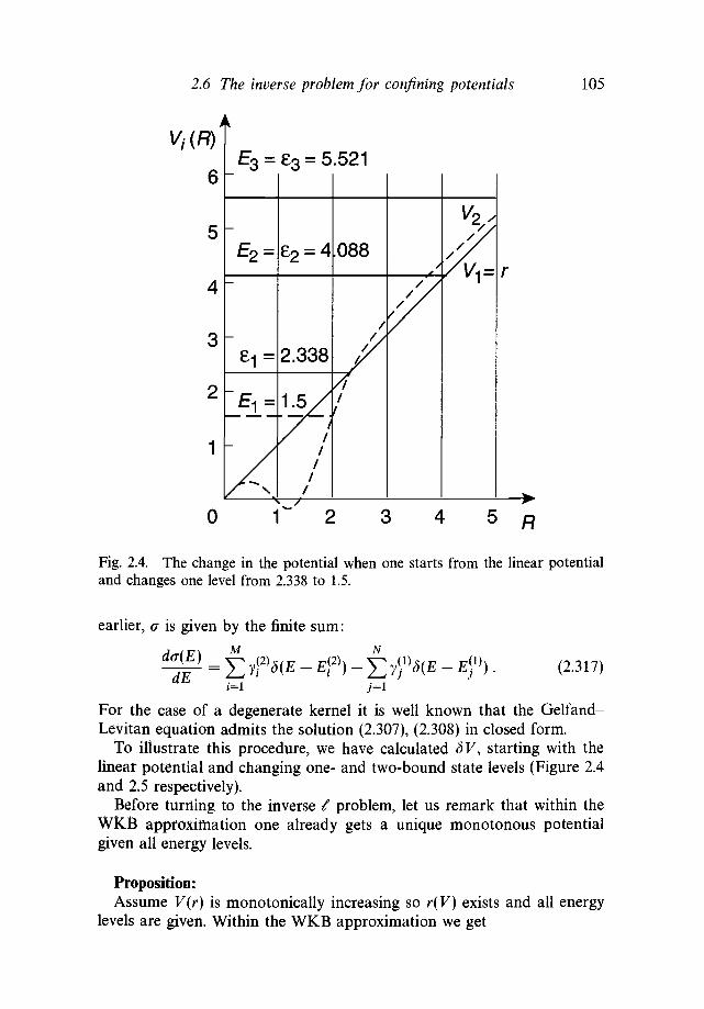
2.6 The inverse problem for confining potentials 105
5
4
3
2
1
0
E2 =
£1 =
J±z
£3 = 5
£2 = 4
2.338
.521
.088r
Fig. 2.4. The change in the potential when one starts from the linear potentialand changes one level from 2.338 to 1.5.
earlier, a is given by the finite sum:
da(E)=M ,dE ^ 7 i
N(2.317)
For the case of a degenerate kernel it is well known that the Gelfand-Levitan equation admits the solution (2.307), (2.308) in closed form.
To illustrate this procedure, we have calculated dV\ starting with thelinear potential and changing one- and two-bound state levels (Figure 2.4and 2.5 respectively).
Before turning to the inverse t problem, let us remark that within theWKB approximation one already gets a unique monotonous potentialgiven all energy levels.
Proposition:Assume V(r) is monotonically increasing so r(V) exists and all energy
levels are given. Within the WKB approximation we get

106 Two-body problems
A
8 2 =
~E2 =
-Jlr.
e3 = 5
4.0883.5
2.338
/
.521
7 /
yr
—w
Fig. 2.5. The variation in the potential due to changing two levels.
(a) for the S-wave case [114]:
J En
dE'
(b) for the three-dimensional case:
r j (F ) -6
1TF d£' '
dE>ro dE'2
(2.318)
(2.319)
Proo/:
(a) The number of bound states below some energy E is given in thesemiclassical approximation by
(2.320)

2.6 The inverse problem for confining potentials 107
Differentiating N(E) once, with respect to £, we get an expressionwhich can be regarded as an Abel integral equation for r(V) andinverted; this gives (2.318).
(b) To proceed similarly in the three-dimensional case, we use the well-known formula for the total number of bound states below E:
^ -^ [ d3x(E - V{r)f'2 .6nz J
N(E) ^ -^ [ d3x(E - V{r)f'2 . (2.321)6nz J
It was first shown in Ref. [121] that (2.321) becomes exact in thestrong coupling limit, where one takes kV(r) as a potential and takesthe limit X —> oo. To invert (2.321), one differentiates twice and againgets an Abel integral equation:
6TT J(fiN \ f dVdr\V)/dV
] (E - (2.322)
Inverting (2.322) gives (2.319).
Remark:The obvious generalization of (2.321) to different 'moments ' of sums
over energy levels — or, rather, quantities like Tr#(—f/)|H| a — has beendiscussed in the literature (see e.g. Ref. [127]: there also exist rigorousbounds of that type,
Et\a < Ca [d3x\V-(x)\3/2+a , (2.323)
where \V-\ denotes the absolute value of the attractive part of V. Suchbounds have led to the creation of a whole 'industry', since it was recog-nized that they are of great help in the problem of proving the 'stabilityof matter' (see Section 2.7)
The inverse problem for
We now want to discuss a non-standard inverse problem connected withconfining potentials. Instead of giving ourselves the successive energylevels for a given angular momentum, we give ourselves the ground-state energies for all physical angular momenta, £(/) . The question iswhether this uniquely fixes the potential or not. We shall not be able togive a complete answer to this question, but collect a certain number ofindications towards the following conjecture:

108 Two-body problems
Conjecture:The confining potential is uniquely fixed by knowledge of the ground-
state energies of the system for all angular momenta.
Example:First, we look at a particularly simple case, that of equally spaced energy
levels
A + Bt. (2.324)
One solution of the problem is well known. It is the harmonic oscillator
V(r) = ^r2 + A - ^ . (2.325)
For this particular solution of the inverse problem, the reduced wavefunctions associated with £( / ) are given by (in the special case of B = 2)
u<(r) = i V m e x p ( - r 2 / 2 ) . (2.326)
We shall content ourselves with investigating the local uniqueness ofV. Suppose we change the potential by bV, infinitesimal. Then by theFeynman-Hellmann theorem the change in the energy levels will be
SE;= IdrdV\uj(r)\2 . (2.327)Jo
An equivalent potential V + SV will be such that all SE^ vanish. Thequestion is then one of completeness. From (2.326) and (2.327) we have,putting r8V(r) = W(x\r2 = x,
L dxW(x)x^e~x =0, V / e N . (2.328)o
According to Szego [122] the system fa = xfe~x is 'closed', so that anyfunction f(x) = W(x)e~x, with a finite L2 norm, can be approximated by][](7(/v in such a way thatII f(x) ~ Z^c/</v II2< ? with e arbitrarily small. That we need an as-sumption on W(x) can be seen from observing that the system of powersxk,k = 0,1,2,... is not complete with respect to a weight exp (— In2 |x|)[123], since
dxxke-ln2 w sin(27c In |x|) = 0 (2.329)o
for all k. This means that any function which has arbitrarily close mean-square approximations by means of polynomials for the above weight isorthogonal to sin (27cln |x|). This example is due to Stieltjes.

2.6 The inverse problem for confining potentials 109
If 8V grows more slowly than any exponential, f(x) is guaranteedto have a finite L2 norm and the theorem applies. Conditions (2.328)therefore guarantee that 8V = 0. Thus we get the following proposition:
Proposition:If the levels £(/) are equally spaced, the harmonic oscillator potential
constitutes an isolated solution to the inverse problem.If one tries to generalize this result to other potentials one first gets the
set of equations
rJo
= 0, V / G N ;
however, one encounters a very difficult problem, which is to prove thatthe set of functions \u<?(r)\2 is complete in some way; the mathematicalliterature is incredibly poor in this respect.
We shall nevertheless try to study these functions |iv(r)|2 and prove thefollowing proposition:
Proposition:Let V(r) be a confining potential such that V(r)/r2 —> 0 for r —> oo.
Then the reduced wave functions uj(r) associated with the levels £(/),normalized by limr_>o us(r)/r'+1 = 1, are such that for any fixed R
and
Proof:We incorporate the normalization condition by writing the integral
equation
u'AR) = 1
+ Wo[V(r')-E(f)]. (2.330)
We define Re to be the smallest r such that E = V(Rc). If r < Re we havefrom Eq. (2.330) u^(r) < r/+1 and, by iteration,
Mr) >
and hence
Mr) 1 -2/
(2.331)
(2.332)

110 Two-body problems
Since, as we have seen from the considerations in Section 2.3,
27TI-0 if i ^ ^ ° forr^°°'the first part of this proposition follows. The statement about the derivativeof U{ follows by differentiating (2.330). •
Remark:We believe that the last proposition is indicative that the set of functions
uj(r) is in some way complete, at least on a finite interval. According to atheorem of Miintz [124], a sequence of pure powers ran is complete if theocns have a finite density for n —• oo. However, even if we were to succeedin proving completeness over a finite interval, we would have the problemof letting the interval extend towards +oo.
We shall, however, make another completely rigorous use of the lastresult, but restrict the generality of the possible variations of d V.
Theorem:Assume that the set of levels £(/) is reproduced by two potentials, U
and V, such that U/r2 and V/r2 -» 0 for r —• oo, and U(r) and V(r) -» oofor r —• oo. If, in addition, U — V has a definite sign for r > R, then U = Vfor r > R.
Proof:Consider a given energy level £(/). The wave functions, normalized
as in the last proposition, associated with the potentials U and V are,respectively, uj and iv- By combination with the Schrodinger equation onegets
/•oo rR\iflt - UfV; \R= (V - U)ufVfdr = /
JR JO- V).
Assume that for r > R, V — U has a constant sign which can be chosento be positive. We then have
u'w - u,v', \R> / druMV -U\ e > 0 . (2.333)
For large t the last proposition allows us to estimate both sides of (2.335).The l.h.s. is of the order of (2/ + l ) # 2 m , while the r.h.s. is larger than
r(l+2e)Rdr(V-U),//
J{l+c)R
which is clearly a contradiction, unless V = U for r > R.

2.6 The inverse problem for confining potentials 111
Now we are working with a compact interval and we have two possi-bilities, one being rigorous, the other imperfect. •
Corollary to the last theorem:If, in addition, V — U has a finite number of changes of sign, V = U.
Proof:First apply the theorem to Rn, corresponding to the last change of sign
of V - U, then to Rn-u etc. •
Pseudocorollary:We keep the conditions of the last theorem. We admit that we have
conditions sufficiently close to the Muntz theorem to believe that the setof the u/vs is complete on a finite interval and conclude from J0
K dr(U —V)uw = 0 that U = V.
This is as far as we have been able to go on a completely rigorous basis.Now we shall describe a semiclassical treatment of the problem. Assume
for simplicity (d/dr)[r3(dV/dr)] > 0. This guarantees that / ( / + l ) / r 2 + F(r)has a unique minimum. It also implies that V is increasing.
We start by purely classical considerations, neglecting completely theradial kinetic energy. Then £( / ) will be the minimum of the centrifugaland the potential energies
E(£) = if + l/2)2/r2 + V(r), (2.334)
with r given by
2{t + l /2)2/r3 = dV/dr , (2.335)
r being a function of / . We can differentiate £( / ) with respect to / , usingan interpolation in *f, taking into account (2.333) and get
,2336,r2
Remark:r2 can be rewritten as (d£/d[/( /+l)])~ 1, which, according to the general
concavity property, is an increasing function of / .With r being given as a function of / , V can also be obtained as a
function of / , from (2.334)
V(S) = £(/) - \ (V + 1 ) &EIU . (2.337)
We see that at this level the inverse problem is incredibly simple. We shalltry to see to what extent this kind of approach can be justified quantum

112 Two-body problems
mechanically. Interpolation in £ is not a problem. It was done long agoby Regge [125]. We shall return to this problem in the next section.
The quantum mechanical analogue of (2.334) is
E(f) = j T dr [«* + ^-±i>«* + V(r)uj\ , (2.338)
where from now on we take uj to be normalized by /0°° druj = 1. Hencewe get, using the well-known inequality /0°° dru2/4r2 < /0°° drua9
> min ((f + l) /r2 + V(r)J (2.339)
which very much resembles (2.334), except for the fact that it is aninequality. The quantum mechanical analogue of (2.336) is
dF r°° u2— = ( 2 ^ + 1) / dr-, (2.340)d£ Jo r2
and, if the wave function is sufficiently concentrated around the minimumof the effective potential, reduces to (2.336). Our condition on the potentialin fact allows us to make a very precise statement.
Proposition:Define ro and r\ by
= / dr-%, V(n)= dru2V(r) (2.341)
rg JO rz Jo
and assumed <JdV\^n
then r\ >
Proof:We shall be satisfied by proving r\ ^ TQ. If r\ =
rJo
( 1 3 4 2 )
Calling the curly bracket y(r) we see that y(ro) = yr(ro) = 0, but (d/dr)r3
(dy/dr) > 0, which guarantees y(r) > 0. The sign of the inequality betweenro and r\ is intuitively clear. •

2.6 The inverse problem for confining potentials 113
Remark:From the last proposition, we conclude that:
i AV !2/ 4- 1^ P.343)
This can be made more practical by using concavity in / ( / + 1) andavoiding the use of non-integer /.
We have
1)] > > ^ Ja r 2^ + 3
and hence we get the definition and the inequality2/ — 1 1 1 / -h -
I(2.345)
This is a strict and probably useful inequality, but it does not tell us howclose we are to the potential.
Now we shall abandon rigour and try to approximate the effectivepotential / ( / + l) /r 2 + V(r) by a harmonic potential and calculate thezero-point energy. To make this estimate, we use the potential determinedwithout quantum effects and compute the curvature at the minimum. Thisgives
Vir\ _ p(/\ W + l) dE
= mfh
Unfortunately, it seems difficult to find a systematic iterative procedureto improve this formula. As it stands, it gives rather good results for larger.
Example:Take Eo = If + 3 (V = r2). Equations (2.343) give V = r2 + 1, while
Eqs. (2.346) give
and therefore there is no constant term.

114 Two-body problems
Example:Let
Equations (2.346) give
while (2.343) contains, after the leading term, a contribution in r~3//2.Our conclusion is that empirically our improved semiclassical procedure
is excellent for obtaining the large-distance behaviour of the potential,and can certainly be used as a starting point in the search for the exactpotential. On the other hand, a very well-posed, but difficult, mathematicalproblem remains.
Regge trajectories for confining potentials
We have previously been led to introduce an interpretation of the ground-state energies for non-integer / . In Section 2.1 we also mentioned convexityproperties in / . Confining potentials are in a way simpler than ordi-nary potentials in regard to analyticity properties in the angular momen-tum complex plane, because of the absence of the continuous spectrum.
Following Regge [125] we can try to solve the Schrodinger equation forcomplex / , with Re / > - 1 / 2 :
d\2
drJ +^2 + V(r)\u(r) EV)u(r)9 l W + l)9 ii(0) = 0.
(2.347)By multiplication by u and integration we immediately get
/ dr\\u'\2+ K 7" }\u\2 + V(r)\u\2\=E(f) dr\u\2, (2.348)Jo [ rz J Jo
which implies that normalizable solutions of the Schrodinger equation aresuch that
Im X \ &rx\ =ImE dr\u\2, (2.349)Jo rl Jo
and hence for real angular momentum E is real. In non-confining, rapidlydecreasing potentials, solutions of the Schrodinger equation for / real andlarge enough, are no longer normalizable, the reality argument breaksdown and, as everybody knows, the energies become complex or, con-versely, real positive energies correspond to complex angular momenta.
We think it is worth studying Regge trajectories in confining potentials,because there are practically no examples of Regge trajectories known,

2.6 The inverse problem for confining potentials 115
except in the oscillator and Coulomb cases, and for numerical calculationsin the Yukawa potential.
The problem is that E(i\ defined implicitly by (2.347), is analyticwhenever the derivative
U2 rco
exists, but except for / real nobody knows when this derivative existsbecause /Q00 druj may vanish. What is known is that if £( / ) — or / (£) —has isolated singularities in the complex / plane, these singularities cannotbe poles or essential singularities because from (2.349) Im E/Im X > 0, orsince Re / > - 1 / 2 , Im £( / ) / Im t > 0.
From now on we shall restrict ourselves to the pure power potentials
V(r) = r« . (2.351)
This will allow us to use the complex r plane. In fact, most of what followsis an adaptation of the work of Loeffel and one of the present authors(A.M.) [81, 126] on the anharmonic oscillator.
For a potential of the type (2.351) the solution of the Schrodinger
equation behaves at large distances like the WKB solution. One can use
the WKB solution as a starting point to establish an asymptotic expansion
of the solution:
"S72TTf(1 + 0(rl~a/2)) f o r a > 2 ' (2352)
{In the case a < 2, more and more terms are needed in the expansion as aapproaches zero, if one wants wo to be such that limr_>oo( /wo) = 1.
Because the potential is an analytic function of z = r except at theorigin, the solution can be analytically continued in the complex r planefor fixed ((real or complex). It can be shown that the solution is decreasingin the sector
n n< arg z <2 + a ° 2 + a
where it behaves like the analytic continuation of (2.352)-(2.354) — i.e.,it is dominated by exp{-z<a/2+1V(a/2 + 1)}.

116 Two-body problems
Remark (a):If a > 2, the two independent solutions behave like
f 7a/2+l ^
-(a/2) + l j
and hence \u\2 is still square integrable along the rays arg z = +n/(2 + a).We shall need to continue the solution in —37i/(a + 2) < arg z <
37r/(a + 2) further. In the sector n/(a + 2) < arg z < 3;r/(a + 2), u is,a priori, a superposition of solutions asymptotically behaving like uo =z-«/ 4 exp(P(z)), v0 = z-«/ 4 exp(-P(z)), where P(z) = - (z a / 2 + 1 / (a /2 +1)) + (£/2)(z1~a / 2/(l - a/2)) + ... contains only positive powers of z. Buttto/t>o —• oo for 7i/(a + 2) < arg z < 37i/(a + 2) and hence \U/UQ\ < const.We get the following situation: u/uo —• 1 for |arg z\ < n/(2 + a), \u/uo\ <const for |arg z\ < min{37i/(2 + a), TT}. According to Montel's theorem weconclude that
u/u0 -> 1 for |arg z\ < min {3TC/(2 + a), n) . (2.355)
Let us now describe our strategy for establishing the analyticity prop-erties of the energy levels En(£) with respect to t or X. We have seenalready that the only singularities to worry about are branch points (nat-ural boundaries can be discarded after a difficult argument which we shallnot reproduce here). To exclude branch points, first find a characterizationof the successive energy levels for complex / . For / real > —1/2 the levelsare labelled by the number of zeros of u(r) on the real positive axis. Thefirst step will be to show that in the angle
|arg z\ < min{7r, 3TT/(2 + a)}
there are no other zeros for real /. We can show that it is still possibleto characterize these energy levels for complex £ by the number of zeroseither in |arg z\ < n/(2 + a) in the case in which a > 2, or in
—- < arg z < for a < 2, Im X > 02 + a 2 + a
and2TT
< arg z < for a < 2, Im X < 0 .z-hoc 2 + a
We shall prove that the number of zeros in these regions does not varyalong any path in the complex £ plane starting from and returning to thereal axis, with Re £ > —1/2. This will demonstrate the absence of branchpoints.

2.6 The inverse problem for confining potentials 117
Step I:/ real > —1/2. The Schrodinger equation written along a complex ray
z = t e1^ becomes
Re u'u =(2.357)
Im u'u = / dt'{t'« sin(2 + a)0 - E sin20}|w| 2 . (2.358)Jo
If |0| < 7i/(2 + a), u —> 0 at infinity and the integration sign /J in (2.357)and (2.358) can be replaced by — /t°°. In this case we see that since theintegrand in (2.358) is monotonous, we can always choose the limits insuch a way that the integrand has a constant sign. Therefore, we have thefollowing:
Property 1:For t real > —1/2, u and u' have no zero in
0 < |0| <7i/(2 + a ) .
We try now to investigate TT/(2 + a) < |arg 0|. One considers the combi-nation
Re(wV)cos /? — sin ft Im(z/w*).
This will be different from zero if one can find /J such that
cos P > 0, cos((2 + a)0 + p) > 0, cos(20 + P) < 0 .
This is possible, if simultaneously
Hence we get:
Property 2:For t real > —1/2 and a < 4, u and i/ have no zeros in
0 < |0| < min(37c/(a + 2),n) .

118 Two-body problems
Step II:We make X complex, for instance, Im X > 0. Equation (2.356) then
becomes
I m u V = / f dt'lMl2 { ^ ^ + ^ sin(2 + a)^ — |£ | sin(20 + arg(2.359)
If 0 < </> < 7i /(2 + a) the integral tends to zero if t -> oo. However,sin(2 + a)(/> > 0; so we conclude sin(2(/> + arg E) > 0. Hence, usingcontinuity we get:
0 < arg E < an/'(2 + a), Im X > 0 . (2.360)
Next, we prove a number of properties of zeros.
Property 3:For Im X > 0, u has no zeros for —n/{2 + a) < (/> < 0.
Proof:For 4> i n that interval the integrand in (2.359) is monotonous and one
can choose the integration limits as (0, t) or (oo, t). •
Property 4:For Im X > 0, a > 2, u has no zero for
Proof:According to Remark (a), \u\ is square integrable and we get
(2.361)Again, since the integrand is monotonous Im u'u* cannot vanish. •
Property 5:For Im X > 0, a < 2, u has no zeros for
$ = 2n/(2 + a).
Proof:Here we can only use the limits (0, t):
Imu'u = J^dtW^-lElsm^^+avgE^ . (2.362)

2.6 The inverse problem for confining potentials 119
According to (2.360) and condition a < 2, we have
n < 4n/(2 + a) < * + arg£ < (4 + oc)n/(2 + a) < In ,\Z* T" QC/
and the integrand in the above expression is positive. •
Finally we notice:
Property 6:u has no zeros for \t\ large enough, and
|0| <min{7i,37r/(2 + a)} .
Proof:This follows from the remark that u/uo -» 1 in this sector and that
has no zeros.
Step III:Continuation in X: We vary X continuously, starting from X real > —1/4
and taking for instance the case of Im X > 0. Initially, from Property 6we know that in the angle \(j)\ < min[37c/(2 + a),7i] if a < 4, \(j)\ <7c/(2 + a) if a > 2, u(r) has only zeros on the positive real axis, (/> = 0, thenumber of zeros (not including z = 0) being equal to n — 1 for the n-thlevel.
Now we distinguish two cases:
(i) a > 2. If we make X complex there cannot be any zero on the lines</) = +7c/(a + 2) from Properties 3 and 4 and no zero can comefrom infinity in the sector |</>| < 7i/(a + 2), from Property 6. Since thezeros are a continuous function of X, their number inside the sector|0| < 7c/(a + 2) is equal to what it was initially, for Re A. If we returnto Re X, we get back to the same energy level, since the number ofzeros has not changed. Therefore, there are no branch points in theX complex plane cut from —oo to —1/4.
(ii) a < 2. Take, for instance, Im X > 0. There are no zeros in — n/(a+2)<(j) < 0, no zeros on the line 0 = 27i/(2 + a) and no zeros at infinity inthe sector 0 < 0 < min{37i/(2 + a),7i}. Therefore, again, the numberof zeros in the sector —n/((x + 2) < </> < 2n/((x + 2) remains the sameas for Re X and continues to characterize the energy levels. Againwe conclude that E(X) has no branch points in the X complex plane,cut from —oo to —1/4.

120 Two-body problems
We conclude with:
Theorem:The energy levels En(£) in a potential V = ra can be continued for
complex / . The functions En(/) are analytic in Re t > —1/2.
Remarks:
We also have the property
Im En(k = t{t + 1))/Im k > 0 ,
which indicates that En(k) is a Herglotz function, which can be written as
r 1 / 4 ^ ' I m
with Im £n > 0. It is easy to check that this fits with the concavity of Enwith respect to / ( / + 1) mentioned in Section 2.1.
However, we have
|a rg£ | <a7c/(2 + a ) .
If a < 2, this means |arg E\ < n/2. We conclude that [En(k)]2 is alsoa Herglotz function, and therefore En(k) increases, at most, like A1//2 ifa < 2. Since (k + 1/4)1/2 = t + 1/2, it is tempting to speculate that foron < 2, £„(/) is itself a Herglotz function. However, we would need toestablish the analyticity of En(f) for Re / < —1/2, and this is difficult.The Herglotz property of En{£) for a < 2 fits with our proposition on theconcavity of En{i) with respect to / .
More generally, [£n(A)]^2+a^a is a Herglotz function, and therefore En(k)cannot grow faster than /2a/(a+2)? for large {. This fits with Equation (2.82).One can also exploit the fact that a Herglotz function is concave, and getuseful bounds for arbitrary n.
Conclusion
It would be very desirable to extend these results to superpositions ofpowers, at least with positive weights. However, it is a weakness of ourapproach that it cannot handle these superpositions, because the variouscritical lines in the z complex plane change with a.

2.7 Counting the number of bound states 111
2.7 Counting the number of bound states
Motivation — History
Many-body problems are not easy to treat in general. But at least somequestions can be handled by studying related non-linear one-body prob-lems. This applies especially to the so-called 'stability of matter'problem.The question is: Why is a system of N particles interacting via Coulombforces stable [5, 6]? Or, expressed differently: Does the ground-state en-ergy per particle converge to a finite limit for JV -> oo? Let us first quotethe many-body Hamiltonian
We are interested in the fermionic ground-state energy £#, correspondingto a totally antisymmetric wave function with spatial part ip(xi,...,Xjv).A very rough simplified argument would be the following: If JV fermionsoccupy a volume V9 the volume available for a particle is of the order ofV/N; let V be a cube of side length R. A characteristic length is thereforeof the order of R/N1^3. From the uncertainty principle we would estimatethe kinetic energy as
N • (pj) N1^r= P5'3R3, (2.365)
where we have introduced the density p = N/R3 which becomes in theThomas-Fermi model the one-particle density
p(xi) = Jd3x2...d3xN\ip(xuh,---^N)\2 • (2.366)
In fact, in the Thomas-Fermi model the kinetic energy is replaced by the5/3 moment of p times a suitable constant:
VlE^lv)^c|rfV/3W. (2-367)
In order to derive (2.367) for an arbitrary antisymmetric xp, we start fromthe Hamiltonian hu = Ylf=i hj, where hj = pj2/2m + V(XJ) and the one-particle potential is chosen to be V(x) = —Xp 2^3(x). From the variationalprinciple we deduce an upper bound on the fermionic ground-state energyEQ ; a lower bound is obtained from filling the one-particle energy levels
-KJ\V{x)\5'2d3x <J2ei^ Eo < (Vlffolv) = T(xp) - X j p5'3{x)d3x.(2.368)

122 Two-body problems
The first inequality of (2.368) allows us to deduce (2.367). This is a crucialstep that has led to a whole industry and many attempts have been madeto obtain bounds of this type. More generally, we may ask for bounds onthe moments of energy levels which are of the quasiclassical phase-spaceintegrals type [127]
J (2.369)
(4n)d/2r (a + 1 + (d/2)) '
In (2.369) we sum over all negative-energy eigenvalues. |K_(x)| denotesthe absolute value of the attractive part of V(x). A simple shift allows usto evaluate the energy levels below a fixed energy.
We note that the quasiclassical limit ft —• 0 is related by scaling to thestrong coupling limit. The first proof that the number of bound statesbehaves as given by (2.367) in one-dimensional Schrodinger problems isdue to Chadan [128]. The general d-dimensional case has been studiedby one of the authors (A.M.) [129]. A further remark concerns relationsbetween different moments . Let us denote by N$ the total number ofbound states below an energy value S. We obtain
ej\" = / dN#\g\« = - r ° dN-$$* = a F dS • S^N-s (2.370)./-oo JO JO
j
and relate an integral over the zero moment to the a moment.We should remark that for a complete solution of the stability problem
an estimate of the potential energy is also needed. The simple-mindedargument would run as follows: Positive and negative charges may bearranged in an alternating way and the averaged distance between nearestneighbours will be of the order of R/N1^. The total energy will thenbehave as
which, optimized with respect to R, yields EN, proportional to N. Butthe estimate of the potential energy is delicate, since N(N — l)/2 termscontribute to (2.364). There is an electrostatic inequality,
N i N
|3c-3c,| 2jUXay\x-y\
-ex f d3xp5/\x) - y c2 , with f £xp(x) = N , (2.372)

2.7 Counting the number of bound states 123
(with c\ and ci suitable constants), which allows binding of the potentialenergy from below. We shall not go into the technical details but just saythat together (2.368) and (2.372) allow us to prove the stability result. Animproved bound of the type (2.368) will also improve the stability bound.
The history of estimates of the type (2.369) can be traced back to aproblem treated by Weyl in 1911: We take as an operator the negativeLaplacian —AQ with Dirichlet boundary conditions on a domain Q a Rd.The number of frequencies Nd(Q X) below the value X grows with X as
Nd(Q,X)^ Xd/2\Q\, (2.373)
where |Q| denotes the volume of the domain Q.A number of semiclassical expansions have been treated in the literature
and have become famous. Kac asked whether one can hear the shape ofa drum. A simple argument shows that frequencies Xm proportional to m2
must come from a circular drum. We expand the trace of the heat kernelof —AQ as
Tr e*> = £ e^< % ^ + ^ + c2 + ... , (2.374)
with known constants Co, ci> C2>.... Here |Q| denotes the area of the drum,L denotes the length of the boundary of the two-dimensional domain,while C2 is determined by the Euler characteristic: If all frequencies areknown, the number of holes in the drum is determined. |Q| and L are ingeneral related by an isoperimetric inequality |Q| < L2/An. This inequalitybecomes an equality if the drum is circular. This essentially proves theuniqueness of the inverse problem for the case of a circular domain. Thegeneral inverse problem is much more complicated and has not beensolved in general.
The analogue of expansion (2.374) for potential problems in onedimension deserves mention, too: For reasons of simplicity we treatH = -d2/dx2 + V(x) defined on a finite interval [0,L], so that H hasa discrete spectrum. The expansion becomes
Tre-tH ^ —Y,c nfln, (2.375)
where In are functional of V(x) and derivatives of V(x): I\ = /0LdxV(x),
I2 = $dxV2{x\ h = fodx(V3 + V2),... and known constants cn. Sincethe spectrum of H is left invariant under the KdF-flow, the functionals/„ are invariant, too, and are related to the higher conserved quantities ofthe KdV equation.
We may add an amusing remark about the stability of the hydrogenatom. We learn in lectures that the uncertainty principle 'proves' that the

124 Two-body problems
hydrogen atom is stable. For h = —A — oc/r the infimum of the spectrum isfinite. The uncertainty principle shows only that the product of the meansquare deviations of the momentum operator Ap times the mean squaredeviation of the position operator Ax is lower-bounded
ApAx > — , (2.376)
and it is amusing to note that there is no way to show, using only (2.376),that (\p\H\p) is bounded from below. A sequence of trial functions whichrespect (2.376), but which lead to expectation values of H that tend to—oo is easily constructed. We take a wave packet which is supported 50%on a big sphere of radius R and 50% on a small sphere of radius s; then(x2) ~ R2/2 but (1/r) ~ l/2e. The expectation value of (if) ~ 2/i?2-a/2ewill tend to —oo for s going to zero, and e and R are unrelated. This showsthat we need a 'better uncertainty principle' which allows stability to beshown. The inequality due to Sobolev from 1938 allows one to do so. Itallows binding of the kinetic energy by a certain moment of the density
d3x\Wxp(x)\2 > I / d3x\xp{x)\6 J , s = —F^ - 0.0780 . (2.377)
More details concerning (2.377) and the evaluation of the Sobolev constants will be given in Appendix C. Here, we cite that the use of (2.377) allows usto obtain a finite lower bound to the ground-state energy of the hydrogenatom
( ( ^ ) | / ( / ) 1 / 3 / ^ | (2.378)
which is finite. The actual value is —1.3 Ry, which differs from the exactanswer by 30 per cent.
A non-trivial lower bound on if = —A + V(x) for potentials which arein a i/-class for p > 3/2 has been obtained by one of the authors (H.G.):
H = -A + V > -CP\\V\\2//{2P~3\ p > 3/2 , (2.379)
where the constant cp is given by2p-2
P-IThe bound (2.379) indicates that the behaviour of a potential at the
origin like V(r) ~ — l/r(2~e) with & > 0 gives a Hamiltonian which islower-bounded.
A combination of the argument leading to (2.377) and Holder's inequal-ity leads to a criterion which allows the exclusion of bound states [130].

2.7 Counting the number of bound states 125
The energy functional may be bounded as
(2.380)
Therefore, if s J d3x\V-\3^2(x) is less than one, bound states are excluded.
Locating bound states
There exist a few general results which help us to obtain insights into anumber of situations.
For example, let us assume that we have two potentials, V\ and F2,which are related such that V\ > V2 for all x. Then the number of boundstates below some energy E for the first problem cannot exceed the numberof bound states for the second case: NE(VI) < NE{V2). This follows fromthe min-max principle (Eq. (2.7)) by taking the true eigenfunctions forthe first case as trial functions for the second. As an application we maycompare a potential problem with potential V\{x) = V(x) to anotherone where only the attractive part of V is taken into account V2(x) =-\V-(x)\ = +V(x)9(-V). Then clearly, V2 < Vx and NE(V) < NE(-\V-\).
Another example is given by taking V\ to be some spherical, symmetric,attractive potential up to a radius R and setting V\ outside infinite, whichmeans Dirichlet boundary conditions. V2 is taken to be identical to V\ upto R, but constant, which we may put to zero, outside. Then, if no is thenumber of bound states with angular momentum zero, no(Fi) < ^0(^2),but no(V2) — no(V\) < 1, too — since the number of bound states equalsthe number of nodes of the wave function for the appropriate energy.
There are a number of ways to estimate how many bound states mayoccur. It depends very much on the dimensionality. A few examples follow.
We have already mentioned that any one-dimensional Schrodinger oper-ator —A+V(x) such that / dxV(x) is negative has at least one bound state.This can be shown by taking a Gaussian trial function cpx = Xl/2e~Xx2 andobserving the scaling behaviour of (q>x\A(px) and {(pi\V(px). The conditionon the integral over the potential is necessary. A counterexample withJ-oo dxV(x) > 0, which does not have a bound state, is given by a sum oftwo 5-potentials V{x) = -X6{x + R) + /ad(x - i?), k > 0, \i > 0, but \i > LIf X is small enough (depending on R) no bound state occurs.
A similar result holds in two dimensions. Any two-dimensionalSchrodinger operator — A + V with / dx f dyV(x,y) < 00 has at leastone bound state. We take again a trial function, this time in the forme~Xr". We obtain an upper bound to the ground-state energy £0 of the

126 Two-body problems
form
N = T + V, (2.381)
^t, ^ - r * I" £dr Jo J-n 2TT
n _ / drre~ Ar
For A —• 0, Vip/Dfa goes to / dx J dyV uniformly for 0 < a < 2.becomes equal to a /0°° du u e~2u by a change of variables and can be madearbitrarily small by taking small-enough a.
Before we discuss methods which allow the counting of bound stateswe may remind the readers of the somewhat surprising remark made in(2.3)-(2.5). Even if a potential goes to zero at infinity (but oscillates) apositive-energy bound state embedded in the continuum may exist.
This can occur only if the potential oscillates at infinity. We pointout that there exist no positive-energy bound states if the potential is ofbounded variation, or is absolutely integrable at infinity, in the sense thatf"\V(r)\dr <ao.
To show this we define the quantity y = ufl + (E — V)u2 and derive fromthe Schrodinger equation that yf = —u 2dV/dr. We consider four cases:
(a) If dV /dr < 0 beyond some value of r which we denote by R, thenyr is positive for all r > R. We can also assume y(R) is positivebecause V goes to zero and E > 0. Hence y(oo) 0, which impliesthe non-occurrence of a bound state.
(b) If dV /dr > 0 beyond R we estimate
/ u2dV/dr dV/dr> —y u2(E-V) + u'2- E-s
for some s > 0, since V —• 0. We integrate (2.382) and obtainln(y(oo)/y(r)) > — (V(oo) — V(r))/(E — s), which again proves theassertion.
(c) If dV /dr changes sign we put \dV/dr\ in the above estimate, and thiscovers the case of a bounded variation.
(d) If we know only that f£ \V(r)\dr < oo, we define Z = u2 + Eu2.Then Z' = u2V. Hence \Z'/Z\ < \V\/E9 and
Z(oo)> exp-4 rk, JRZ(R)
which proves the impossibility of a positive-energy bound state.

2.7 Counting the number of bound states 127
If a Schrodinger operator with a local (scalar) potential has a groundstate then (i) it is unique and (ii) the ground-state wave function will bepositive everywhere.
We have a simple argument proving uniqueness. Assume that there aretwo ground-state wave functions to the same energy EQ :
(_A + V)tpj = Eotpp 7 = 1,2. (2.383)
We may choose \p\ orthogonal to y>2" {\p\\\pi) = 0. If \p\ is positiveeverywhere it follows that \pi has to change sign somewhere. This leads toa contraction to the assertion that the ground-state wave function has tobe positive. We still have to show the last assertion: the simplest situationis given in one dimension. Assume the ground-state wave function xp(x)changes sign. We take \xp8(x)\ as a trial function where s indicates a smallsmoothing procedure to round off the edge one obtains for \xp(x)\. Oneloses a contribution to the kinetic energy proportional to 5{T) ~ — s • / ,where £ denotes the length of the region where we modified |v>(x)|, while5(V) ~ |a|2. Putting both together we realize that we decrease the energyby taking |y>fi(x)| as a trial function and that this is positive everywhere.A small variation of the argument applies to any dimension.
Birman-Schwinger bound
A certain bound on the number of bound states due to Birman andSchwinger is easy to obtain and is often helpful (see, for example, Ref. [67]),but has the wrong strong-coupling behaviour for large coupling. Wetransform the three-dimensional Schrodinger equation for bound statesinto an integral equation,
^ I e ^ ( 1 3 8 4 )where —K 2 = £, and we assume that V is purely attractive. Otherwise Venters into (2.384) and N(V) < N(V-). We next define <£ = y/V xp andtransform (2.384) into an integral equation, which has a symmetric kernel,
K(x,y)
(2.385)
Instead of considering the dependence of eigenfunctions as a function ofenergy, we can introduce a coupling constant X into (2.385) and study thecharacteristic values X\:
J (2.386)

128 Two-body problems
As a function of X[ the eigenvalues move monotonously. If they crossX — 1 they really represent eigenfunctions of the original problem. Insteadof count the number of eigenvalues below zero energy of the originalproblem, it is equivalent to count the number of characteristic values X[greater than X = 1. Therefore, the trace of X, being the sum of A,-s, will givean upper bound on N. Since that trace turns out to be infinite, we maybind N < J2i f by the Hilbert-Schmidt norm, which is easily calculatedand yields
d'xd'y \V(xW(y)\N f* J
It can be also shown that if (2.385) is finite, the total cross-section atpositive energies is finite [131].
'Quasiclassical' estimates
The quasiclassical limit h —• 0 for Schrodinger potential problems corre-sponds to the strong-coupling limit X —• oo, if we take XV instead of V asa potential. As already remarked (see (2.369)), we expect that all momentsof energy levels will converge towards their classical phase-space integral.The main question now is whether inequalities of the type (2.369), withconstants which might be equal to or greater than C/a^, will hold. For anup-to-date review of this problem see the excellent article of Blanchardand Stubbe [132]. With the help of the Birman-Schwinger technique [127]the following result was obtained:
Theorem:Let |7_ | € La+d/2(Rd) and a > 1/2 for d = 1, a > 0 for d > 2, or
a > 0 for d > 3. Let ej < 0 be the negative-energy bound states ofH = —A + V(x). Then there exist finite constants Laj, such that
Yl N / (2.388)j J
holds.
Remarks:It is trivial to see that there cannot be a bound of the form (2.388) for
d = 1 and 0 < a < 1/2. Consider a potential like v€(z) = 9(e— \z\)/2e: fore —> 0, v€(z) goes to a <5-function potential with exactly one bound state,while the phase-space integral goes to zero. The same argument impliesthat the number of S-wave bound states no for the three-dimensionalSchrodinger problem cannot be bounded by the 11 V\ | / 2 norm. A solution

2.7 Counting the number of bound states 129
has been found by Calogero and Cohn [133], who obtained a bound formonotonous potentials:
2 f°°dr\V{r)\1'2 . (2.389)
2 f°-n Jo
Only for certain values of a and d are the best possible answers to (2.388)known. Much effort was put into obtaining the best answer, for d = 3 anda = 1 and a = 0. In the latter case, one looks for a bound of the type
N3<C fd3x\V-\3/2 . (2.390)
The classical value is C/o,3 = l/6n2 ~ 0.0169. The conjecture is that theSobolev constant is the best possible answer: K = 1/3^/3 (2/n)2 ~ 0.0780.The best-known constant in an inequality of the form (2.390) is due to Lieb[134]: 0.1162 ~ 1.49 K. For the spherically symmetric problem we shallreview our bound [135], which yields 0.1777 as a constant in (2.390). Liand Yau [136] obtained 0.5491 and Blanchard, Stubbe and Rezende [137]0.1286.
Counting the number of bound states for spherically symmetric potentials
If the potential is rotationally symmetric (for reasons of simplicity letus treat the three-dimensional case) there is a simple way to count thenumber of bound states. The zero-energy wave function will divide thehalf-line into n + 1 parts through the positions where it vanishes. Thisnode theorem holds only for d = 1 and half-line problems. We may usethe inequality leading to (2.380) for each interval [rn,rn+i] determined bythese zeros, and obtain inequalities which, summed up, give
„ < „ Jo™ dr(r 2Vf ( p - 1 ) ^n / S p * l S =
Note that the Sobolev constant entering (2.377) is related to S3/2: 47rS3/2 =s. We wrote down the generalization taking into account angular momen-tum contributions and using Holder's inequality for index p (see AppendixC). For p = 1 we obtain the old well-known bound of Bargmann. p —• 00gives a result of Courant-Hilbert.
In Ref. [135] a different way of counting the number of bound statesis shown. Let us consider a rotationally symmetric problem and study thebehaviour of eigenvalues as a function of (\
- V(r)) um/(r) = sm/um/ . (2.392)
The total number of bound states is given by N = J2A^ + ^)nt\ f°r
fixed m there is a maximal number of t such that the m-th eigenvalue

130 Two-body problems
disappears in the continuum. Let us denote this value as /m with [/m] asthe integer part of tm. Now we may count multiplicities: between [/m]and |ym-i] + 1 we count (2/ + 1) x 1 bound states; between [/m-i] andVm-i\ + 1 we count (2/ + 2) x 2 bound states and so on. Summing givesa formula for N where no approximations are involved (for d = 3),
l)\ (2.393)
where ,-s are determined through the zero-energy Schrodinger equation
As is well known, we may map problem (2.394) onto a problem definedon the full line z £ (—00,00) by transforming from (r,M,-) to (z, </>,) withz = lnr and <f>i(z) = (l/y/f)ui(r). We obtain
^ Uz)' ( 2 ' 3 9 5 )
where we have written the general case for any d > 2. Since in d = 3 wemay bind (2.393) by
^2 i, (2.396)
where the e s are the eigenvalues of the one-dimensionnal Hamiltonian(2.395), the problem of obtaining bounds on the number of bound statesin three dimensions is reduced to the problem of binding the first momentof energy levels in one dimension. But this can be done as described inRef. [135]. Altogether, we obtain the result
JV3<K /Vx |F_ | 3 / 2 , (2.397)
with K ^ 0.1777, which is to be compared with the (probably best) answerof 0.0780.
As an aside we note that the analogue of (2.396) in d = 4 yields
N4 < J2 N3/2 < Yeldzv2{z)' (1398)
The second inequality in (2.398) comes from a sum rule [138] known tobe optimal for reflectionless potentials. The bound in four dimensions istherefore optimal.
Next we mention the generalization of the above procedure to d di-mensions. As a first step we relate Nd, the number of bound states in apotential problem in d dimensions, to a one-dimensional moment problemfor energy levels.

2.7 Counting the number of bound states 131
For a rotationally invariant potential the reduced wave functions, anal-ogous to (2.392), fulfil the equation
2£ ) p.3,9)
The degeneracy of each level is determined by the number of harmonicpolynomials of degree t in d dimensions D/ = H<? — H<?-2, and the numberof homogeneous polynomials of degree ( in d dimensions is given by
Now we again count multiplicities. If tm still denotes that angularmomentum for which the m-th eigenvalue disappears in the continuumwe obtain
As a second step we transform the problem into a purely one-dimensionalone and obtain (2.395). Let us denote by ex = —{t x + (d - 2)/2)2 theeigenvalue of the one-dimensional problem corresponding to angular mo-mentum tft. Next we bound (2.400) by
In order to proceed, we need bounds on moments of order 3/2, 2, 5/2, 3,etc. in one dimension. Aizenman and Lieb [139] proved that all moments ofthis type of order bigger than 3/2 are less than or equal to the appropriateclassical constant times the appropriate moment of the potential:
[dx\V(x)\ a+l2, a > 3/2 (2.402)
has already been given in (2.369). The inequalities (2.401) and (2.402)together yield our results. For dimensions up to 20 they are summarizedin Table 7.The bounds thus obtained are compared to the one-particle bound Sd ford < 1 and to the classical bound CY<j for d > 8. The bounds are for alld > 5 larger than Sd and CY<j. Furthermore, for d > 7, the maximum ofthe r.h.s. of the expression determining Kj in Eq. (2.401) is reached for an/ value which is non-zero. Indeed, we even found calculable examples ofpotentials which show that for d > 6 the upper bound on Nj is necessarily

132 Two-body problems
Table 7. Illustration of inequality (2.401) and Eq. (2.407): Examples and boundscompared to the Sobelev and classical constant.
d mopt Ex/Sd Ex/C£d /Opt Bound/S^ Bound/C/^
3 1 1 0 2.284 1 1 0 15 1 1 0 1.086 1 1 0 1.127 3 1.16 1 1.23
891011121314151617181920
46810131620242832374247
1.361.291.241.211.181.161.151.131.121.111.111.101.09
2457101316192327323742
1.421.331.271.231.211.181.161.141.141.131.121.101.10
above the classical bound, but approaches it for d —> oo. This disprovesa conjecture of Lieb and Thirring[127]: the belief was that there exists acritical value a in (2.388) called OLC4, such that
= L\d for a < aCyd and L^d = Lcad for a > occ4 , (2.403)
where h\d denotes the optimal constant in (2.388) for N = 1 and Lcad
denotes the classical constant. It has been proven that ac?i = 3/2; it wasconjectured by numerical experiments that aC)2 = 1.165 and ac,3 = 0.8627.We shall describe the examples which disprove the conjecture for a = 0and d > 1 in the next subsection.
A variational approach
We have also tried to obtain an optimal result. In principle, we intendto evaluate a supremum of a certain functional, overall potentials whichsupport a number of bound states. If we fix this number Nd we thereforewould like to obtain the inf y J ddx V(x)d^2. It is clear that there has toexist at least one zero-energy bound state. Otherwise we could decrease

2.7 Counting the number of bound states 133
the coupling constant, changing the above-mentioned functional withoutchanging the number of bound states. Let us assume that this zero-energybound state occurs for angular momentum L. The variational principlewhich we arrive at reads
8 f ddx V(x)d/2 > 0, SEL = f ddx xp2L{x)d V < 0 , (2.404)
where EL denotes the eigenvalue of the particular bound state. Variationof V has to be such that this bound-state energy remains zero or becomesnegative.
We introduce a Lagrange multiplier and derive the proportionality(d2)/2 __ COnst|i/;|2. This implies a scale (and conformal) invariant
non-linear field equation for the zero-energy wave function xpi:
- A V L - |V>LIW~2)V>L = 0 . (2.405)For d = 3 all solutions of (2.405) are known. L = 0 gives the optimalanswer and the Sobolev constant results in the bound for N^ Unfortu-nately, there may also be other solutions to a variational principle withmore zero-energy eigenvalues with angular momentum L7. The resultingnon-linear equation, replacing (2.405), becomes
/ \ 2/(d-2)
- AWLi - I ] T I VLj\2 I WU= 0 . (2.406)
We obtained a number of interesting solutions to (2.406) by projectingstereographically onto a d-dimensional sphere and using the completenessproperty of spherical harmonics on that sphere. With the help of thesesolutions we have been able to gain insight into the questions asked, butthe proof that we have obtained all solutions relevant to the problem hasnot been given.
As we have already mentioned, there may occur a number of zero-energy states for certain angular momenta. We can now sum up themultiplicities following (2.400) and obtain for m zero-energy bound states
Nd = 2d-\d + m-2)\{d + 2m-2)Id CSd p + 2m- 2)(d + 2m- 4)]i(m - 1)! '
where Id = j™ (Xidz\v(z)\dl'1. The results of the optimization in m are alsogiven in Table 7. For 3 < d < 1 we have to compare these with the Sobolevconstants S^ For d > 1 our examples violate the Sobolev bound whichwould result if the nodal theorem were true. We believe that the numbersobtained from (2.407) after optimization of m are the best possible ones.So the new conjecture is that up to d = 6 the Sobolev constants will be thebest possible. For larger d the best answer will be given by the optimizingthe m in (2.407) and for d —> oo the classical value will be reached.

134 Two-body problems
It should be noted that the optimal answers to the mentioned boundsin d = 3 are still missing. In d = 4 the system (2.406) has been shown to becompletely integrable [140]. This field theory is related to the conformalinvariant instanton equation.
Number of bound states in oscillating potentials of the Chadan class
We have already mentioned in Section 2.1 that there is a class of oscillatingpotentials for which the Schrodinger equation is perfectly well behaved.This class was discovered by Chadan [66] some years ago, and, from thepoint of view of principles it is remarkable, because what Chadan requiresare integrability properties of the absolute value of the primitive of thepotential rather than of the absolute value of the potential itself. Here, weshall restrict ourselves to potentials oscillating near the origin and goingto zero sufficiently rapidly at infinity (though one can also consider thecase of potentials oscillating at infinity [141]). In this case one defines
/•GO
W(r) = / V(r')dr' (2.408)
and the Chadan class is defined by
riimr-*rJF(r) = 0\ Ir I W{r')\drr < oo for r -> 0 . K }
We see that ordinary potentials such that V ~ ra for r —> 0 with a >—2 will satisfy these requirements. If, in addition, we require |W(r)| <r~e for r —> oo, we have all desired properties and, in particular, all boundstates have negative energy.
We shall show that it is very easy to get bounds on the number of boundstates in potentials of the Chadan class [142]. Suppose the zero-energysolution of the Schrodinger equation which is regular at the origin has nnodes — i.e., we have n bound states. Consider the interval r^<r < r^+iwhere r& and r^+i are successive nodes. Then, integrating the Schrodingerequation from r& to r^+i, we get
frk+l n f'k+l (£U + 1) \ ~0 = / ua(r)dr + / ^ P + V(r) u\r)dr .
Jrk Jrk \ r JWe then integrate by parts using the definition of W, noting that theintegrated terms vanish:
0 = r+1 \u'2{r) + ^ V(r)1 dr + 2 fM W(r)u(r)u'(r)dr (2.410)
and use the inequality
|2W(r)M(ry(r) | < ^\u'(r)\2 + 2\W(r)u(r)\2 .

2.7 Counting the number of bound states 135
Hence we haverk+i n , i
0 > / Uu'(r)\2-
or0 > / ""* ||f/(r)l2 + "V^2
T u2(r)-A\W(r)\2u2(r) dr , (2.411)
with L(L+1) = 2/(/+l). Inequality (2.411), seen as a variational inequality,means that inside the potential — 4| ^(r)!2, with angular momentum L, andwith Dirichlet boundary conditions at r^ and rk+u there is one negative-energy bound state. Hence, any one of the conditions (2.391) applies withthe necessary substitutions of t by L and \V\ by AW2. For instance, wehave
ArW2(r)dr > 1 ,2L + 1
and reexpressing L and adding up all the intervals we get1n/ <
and similarly16
<3V3TT 8(^
In fact there is some sort of self-consistency: if V is purely attractive— i.e., negative — W(r) is negative, monotonous increasing. Hence, theCalogero bound
2 r00 ino<- J\U(r)\dr,n Jo v
which is valid for a potential U(r) negative, monotonous increasing, ap-plies. So we get
no<- \W(r)\dr = - / r\V(r)\dr ,n Jo n Jo
which is, except for a factor larger than unity, the Bargmann bound.These bounds are not exactly optimal. Bounds with optimal constant
can be found in original references.

Miscellaneous results on thethree-body and A/-body problem
The successful application of the Schrodinger equation to quark-antiquarksystems implies, unavoidably, that one should also apply it to baryonsthat are systems of three quarks, and which, because of 'colour', are notconstrained to have an antisymmetric wave function in spin and space.In fact, historically it was rather the contrary, in the sense that the quarkmodel was first applied to baryons [13]. We shall not describe here thedetails of the model calculations, but shall rather describe some generalproperties coming from the belief that forces between quarks are flavour-independent, as well as from the postulate that the Schrodinger equationholds.
We have said already that if a Hamiltonian is of the form H = A+XB itsground-state energy is concave in X — i.e., d2E(X)/dX2 < 0. A very simpleapplication to the two-body problem [101], [143] is that the binding energyof a system Q1Q2 whose Hamiltonian is
1
is concave in [m^1 + m^1]"1. This means thatF >EQiQi ^
and, adding the constituent masses,
This inequality works very well. For instance, assuming that spin-dependentforces do not cause complications, we have
MD* = 2.12 GeV > UMJ/XP + M+) = 2.06 GeV .
The same concavity property applies for three-body systems — for
136

3.0 Miscellaneous results on the three-body and N-body problem 137
instance, baryons made of three quarks. In particular, E(Qu qi, #3), thebinding energy of a system of one heavy quark and two light quarks isconcave in l /m^ , since the Hamiltonian is
- ^— Ai - - i - A2 - - L A32niQl 2mq2 2mq3
If one has a model giving constituent quark masses, one can in this wayget an upper bound for the mass of a baryon containing a b-quark whenthe masses of the similar baryons containing c- and s-quarks are known.For instance:
{MAc - mc) (l/mc- l/mb) _ (mA - ms) (l/ms - l/mb)l/ms — l/mc l/ms — l/mc
and with ms = 0.518 GeV/c2, mc = 1.8 GeV/c2, mh = 5.174 GeV/c2 [34],this gives a reasonable value, Ref. [144],
MAb < 5.629 GeV/c2
and similarly
< 5.826 GeV/c2 .
At present, experiments give a mass of 5.625 GeV for the A^ [145].It is very tempting to go further in these concavity properties, and
change all masses in
H = - ^ - A i - ^ - A 2 - - i - A 3 + Vn + V1Z + Vl3 . (3.4)2m 2m 2m
Richard and Taxil [44] have observed that the members of the Sl/3decuplet
(qqq)A(s qq)E(s sq)Z*(sss) Q~
have an energy and a mass which is a concave function of the strangenessof the baryon for a 'reasonable' potential (with no spin-dependent forces)— i.e.,
E(mu m2? m2) > ^[E(m2, m2, m2) + E(mu mu m2)] . (3.6)
But what is 'reasonable'? Some 'general' incorrect proofs were proposed,but in the end Lieb [45] gave a proof for a restricted class of potentials.This class is such that

138 Miscellaneous results on the three-body and N-body problem
should have a positive three-dimensional Fourier transform; two sufficientconditions for this to hold were proposed by Lieb.
(a) V, considered as a function of r2, should have successive derivativeswith alternate signs [45] (dV/dr2 > 0 etc.) ;
(b)
V > 0, V" < 0, V" > 0 , (3.7)
a condition previously proposed by Askey [146].
In fact, condition (b), as shown by one of us (A.M.) [147] can beslightly weakened:
(c)
V1 > 0, V" < 0, rV" - V" > 0 . (3.8)
This latter condition is optimal in a certain sense that we shall ex-plain. Let F be such that F > 0, Fr < 0, F" > 0. Then, by successiveintegrations by parts, the three-dimensional Fourier transform ofF, F(q) is found to be proportional to
, 0
JoF " ( r ) F'"(r)^ [qr(l+cosqr)-2 sinqr]2
) 1+cosgr '
If the support of F" — rFr" is restricted to points where the squarebracket vanishes, the Fourier transform vanishes.
Naturally one can ask oneself if for some potentials not satisfying theseconditions the concavity property could be violated. As shown by Lieb inthe extreme case of one particle of infinite mass and a square well thisis the case. It is also the case as shown analytically by Richard, Taxiland one of the present authors (A.M.) [44] for a potential V = r5, andnumerically for V = r26.
These potentials, however, are not 'physical', since they are not concavein r [46]. Yet the weakest condition found involves the third derivative ofthe potential. It is not known if this is due to a deficiency of mathematicalphysicists or if it is deeply needed. We tend to favour the former assump-tion. The 'equal spacing' of the decuplet results from a compensationbetween the concave central energy and the spin-dependent forces.
It is tempting to go further than (3.6), following the suggestion ofRichard, and try to prove the inequality
, m2, m3) > -[E(mu mi, mi)+£(m2, m2, m2)+E(m^ m3, m3)]. (3.10)

3.0 Miscellaneous results on the three-body and N-body problem 139
This turns out to be very easy to prove [148], using the method of Lieb[45], who was able to prove an inequality more general than (3.6):
E(mu m2, ra3) > -[E(mu mu m3) + £(m2, m2, m3)] , (3.11)
under the same conditions — (3.8) for instance. It is also possible to findcounterexamples with sufficiently rapidly rising potentials — for instance,V(r) = r49.
Other very interesting inequalities on three-body systems can be ob-tained if one accepts a not completly justified assumption: in a baryon thequark-quark potential is related to the corresponding quark-antiquarkpotential by
VQ.Q2 = \VQIQ2. (3.12)
The basis for this 'belief is that it holds for the one-gluon exchangepotential. Also, if in a baryon two quarks are close to one another, theyform a diquark, which is in a 3 representation, since it must combine withthe representation 3 of the remaining quark. In all respects it behaveslike an antiquark and its potential interaction with the quark is VQQ.Dividing by two as there are two quarks, we get rule (3.12). From aphenomenological point of view, this rule has led to a beautiful predictionof the mass of the Q~ particle by Richard [41] based entirely on thefit [34] of quarkonium, which is M Q - = 1666 MeV/c2 (while experimentgives 1672 MeV/c2).
Once the rule is accepted, it has beautiful consequences. The three-bodyHamiltonian
A + ] > > (3.13)
can be written as
2 I-,"'" ^ ^
with
Hti = — — A,- —A/ + 2Vij. (3.15)2m/ 2mj
Hij is, according to rule (3.12), a quark-antiquark Hamiltonian. We have
inf H123 > ^[inf H12 + inf H23 + inf Hn] .
Now including the constituent masses we get [40]
E{Qu 62,

140 Miscellaneous results on the three-body and N-body problem
and
M(Qu Q2, 6s) > \ [M(Qu 62) + M(QU g3) + M(Q2, &)] • (3.16)
Strictly speaking, this relation holds for particles without spin. But it alsoholds for parallel spins. In this way we get
MA > 3/2Mp ,
In Ref. [149] Richard and one of the authors (A.M.) have been able toincorporate spin as perturbation. One gets:
Spin 3/2 statesQ~ = 1.672 > 3/2 (/> = 1.530A = 1.232 > 3/2p = 1.155r = 1.385 > K* + l/2p = 1.275E* = 1.532 > p + 1/20 = 1.280Th > B* + l/2p = 5.710
Spin l/2,S-like statesN = 0.938 > 3/4p + 3/4TI = 0.681Z = 1.190 > l/2p + 3/4K + 1/4K* = 0.979S = 1.319 > 1/20 + 3/4K + 1/4K* = 1.104Sc = 2.450 > l/2p + 3/4D + 1/4ZT = 2.288Zfe > l/2p + 3/4B + 1/4B* = 5.670
Spin 1/2, A-like statesA = 1.116 > 1/2TT + 3/4K* + 1/4K = 0.863Ac = 2.286 > 1/2TT + 3/4D* + 1/4D = 2.042Ab > l/2n + 3/4B* + 1/4B = 5.379 .
(3.17)We see that the deviations between the l.h.s. and the r.h.s. of Eqs. (3.17)
oscillate between 100 and 250 MeV. The question is whether one can dobetter than this. That is to say: Can we improve the lower bound givenby (3.16)? The answer is yes.
The method we shall use is, in fact, very general and can be generalizedto the iV-body case without the need to restrict oneself to the three-bodycase. However, in its simplest form it works for equal-mass particles. Theunequal-mass case has been worked out completely for the three-bodycase only.
We start with N equal-mass particles. We use the notation E^{M, V) todesignate the energy of N particles of mass M interacting with a potential

3.0 Miscellaneous results on the three-body and N-body problem 141
V. In this language, the previous inequality for equal masses is
£3 ( V ^ > ^£2(M, V). (3.18)
Notice that
EN(M, V) = jEN (j-9 XVs) . (3.19)
The new inequality [9, 150] is based on a very simple identity on thekinetic energy:
X>i - Pjf + ( £ Pi)2 = NJ2P}- (3-20)
Thus, disregarding the centre-of-mass energy (Y, Pi)2 w e c a n writeV), the Hamiltonian of N particles of mass M with pairwise potential V,as
_ 2 (3.21)with (P^L }
but pi — p;- = 2ntj is TWO times the conjugate momentum to ry:
Therefore fcy is a Hamiltonian corresponding to a reduced mass MN/4— i.e., two particles of mass MN/2. Hence we get
EN(M, V) > E2 I -~2~9 VJ . (3.23)
It is easy to see that (3.23) becomes an equality in the case of harmonicoscillator forces [151]. For N = 3 this gives
£3(M, V) > 3E2 (^-M, V) ,
or, using scaling properties,
£3 ( V ^j > 3-E2 Q M , 7) . (3.24)If we compare this with (3.18) we see that M has been replaced by (3/4)M.The mass is reduced and hence the lower bound is higher.
The gain obtained with this inequality can be appreciated both numer-ically and analytically. Numerically, one can calculate extremely accuratevariational upper bounds for power potentials and then compare with theold and new lower bounds. This is done in Table 8.

142 Miscellaneous results on the three-body and N-body problem
Table 8. Ground-state energy £3 of H3 = 2(1/2)p? +(l/2)e(/?)Sr£. compared to the naive limit (3/2)E2(l;rfi), theimproved lower limit (3/2)£2((3/4);r^) and a simple vari-ational approximation £3 obtained with a Gaussian wavefunction.
p-1-0.50.10.5123
2*2(1)
-0.37500-0.657591.853592.750093.507164.55.17584
2*2(1)
-0.28125-0.597461.879162.912963.860135.196156.15098
£3
-0.26675-0.591731.880192.916543.863095.196156.15591
£3
-0.23873-0.579641.882782.925903.871145.196156.17147
Analytically, there are ways to evaluate the difference £2(3/4 M, V) —E2(M, V) by using the inequalities on the kinetic energy derived in Sec-tion 2.4
( T ) > - ( £ p - £ s ) , (3.25)
where Es denotes the t — 0 ground-state energy of a two-body system,and Ep the energy of the lowest / = 1 state, and the property, followingfrom the Feynman-Hellmann theorem:
(3.26)
By including some further concavity properties of fi{T) one can integrate(3.26) and get a lower bound on the difference of binding energy betweena two-body system of two masses (3/4)M and two masses M. This gives
£3 (M9 ^ , VJ = 0 ) + ^ [£2(M, V91 = 1) - E2(M9 V91 = 0)] ] .(3.27)
A rather spectacular application can be made to the Q~ systems: theprevious inequality gave
Ma- > 1530 GeV ;the new inequality gives
MQ- > 1659 MeVto be compared with the experimental value:
MQ- = 1672 MeV .

3.0 Miscellaneous results on the three-body and N-body problem 143
Table 9. Comparison of the various lower bounds forV = r, and masses (1,1, M). We show the ratio E{3)/E{2\The variational bound corresponds to a hypersphericalcalculation up to grand orbital momentum L = 8.
M0.050.10.20.5125
1020
Variational
5.71784.87244.22503.61473.30453.09762.94082.87952.8466
Naive
5.37954.53033.88453.28943.00002.81712.68692.63862.6134
Optimized
5.71414.86934.22203.61203.30193.09532.93862.87732.8444
Table 10. Comparison of the various lower boundsfor V = —r" 1, and masses (1, 1, M). We show the ratio£(3)/£(2)j s o th a t i o w e r bounds become upper limitsand vice versa.
M0.050.10.20.5125
1020
Variational
0.675000.846931.11831.64842.13402.60453.07873.29903.4268
Naive
1.19051.36361.66672.33333.00003.66674.33334.63644.8095
Optimized
0.693320.868681.16091.73412.25002.74273.23413.46203.5944
All this can be generalized to three particles of unequal masses [151].To do this one has to exploit the freedom to add arbitrarily to theHamiltonian terms of the form (P • Za; pi), where
i=\
The results of numerical experiments for power potentials are again spec-tacular, as shown in Tables 9 and 10.

144 Miscellaneous results on the three-body and N-body problem
Now let us return to the general N-body system. A particularly spec-tacular application is that of N particles interacting with a gravitationalpotential [9]:
N n2 N x
with x = Gm2, G being the Newton constant. An upper bound on theenergy of this iV-particle system can be obtained either by taking ahydrogen-like trial function using the variable J2,\rij\2
9 which is good forsmall N9 or a Hartree wave function n,-(/(r,-)), which is good for large N9
when centre-of-mass effects are negligible.This gives
£ 3 < -1.0375 G2m5
EN < -0.0542 N(N - l)2G2m5,
with
f(r) — exp— y/ar2 + b ;
the new lower bound gives
£3 > -1.125 G2m5
EN > -0.0625 N2(N - 1) G2m5 .
We see that the upper and lower bounds agree within 15%, which is ratherremarkable.
To finish this chapter, we would like to present a very interestingand intriguing development due to Gonzalez-Garcia [152]. He combinesinequalities (3.23) and (3.24) with a l / d expansion of the energies, whered is the dimension of the space.
The idea of a l/d expansion is that if we take N particles in d dimensionsd > N9 the system, provided the forces are conveniently scaled (whichis easy for power potentials), is 'frozen', with fixed distances between theparticles. Deviations from these equilibriuim positions can be describedby harmonic motions, giving rise to l/d corrections. There is, so far, norigorous control on these l/d expansions.
The contribution of Gonzalez-Garcia is that the ratio
R _ £ * ( M , V) (329)E2(NM/2, V)N(N - l) /2 v * ;
approaches unity not only when V becomes a harmonic oscillator poten-tial, but also when d —• 00. The idea, then, is to expand JR in powers of l/dinstead of expanding the individual energies. If this is done to the lowest

3.0 Miscellaneous results on the three-body and N-body problem 145
Table 11. Expansion of R of Eq. (3.29) to lowestorder in 1/d compared to the numerical values.
p
- 1-0.5
0.5123
R-l/d
0.9460.98981.00161.001111.0013
^numerical(Table 8)
0.9480.99041.00121.000811.0008
Relative error%o
20.60.30.300.4
non-trivial order in 1/d, it gives the results presented in Table 11 for athree-body system with equal masses, with two-body potential e(fi)rP (seeTable 8).These results are really impressive, even though we have no idea of theconvergence (or asymptotic character?) of the \/d expansion.
Similarly, for a system of particles in gravitational interaction, Gonzalez-Garcia obtains
FKT
lim * = -0.0539,
to be compared with our upper bound, which is —0.0542.It would certainly be desirable to understand the reasons for the success
of the 1/d approach. This is an interesting, but difficult problem.We have presented only a few facets of the three- and N-body problems.
We recommend to the reader the excellent review of Richard [153] onbaryons as three-quark systems.

Appendix ASupersymmetric quantum mechanics
Here we introduce the appropriate algebraic scheme and indicate the con-nection to factorization of Schrodinger operators used in our discussionof level ordering.
We shall start with the simplest system known to physics, namely theharmonic oscillator, which we may call a bosonic one with Hamiltonian
co d2 co 2 / A * x
For reasons of simplicity we have put m = 1/co. We rewrite (A.1) in'factorized' form
HB = <x>[aJa + -) , a = — + x - = , a J = - — + x ) —= ,V 2 / \dx ) Jl \ dx ) Jl
(A.2)where cfl and a denote creation and annihilation operators for quanta ofthe oscillator. Their commutation relations,
[a,at] = l , [HB,J]=a>a19 (A3)
show the 'bosonic' nature of HB- The spectrum and associated eigenfunc-tions are given by
h n G N 0 , a|0) = 0, ^ \ n ) , (A.4)En co(n + h, nGN0,2
where |0) denotes the ground-state vector and co/2 is the zero-point energy.Before we realize the simplest form of a supersymmetry within potential
models, we 'double' the system treated before by adding a second bosonicoscillator:
h = \{p\ + a>hi) + \(Pi + coWi) • (A.5)
This two-dimensional oscillator obviously has an additional symmetry ifCD\ = a>2- Then h is invariant under rotations within the plane, qi,q2,
146

Supersymmetric quantum mechanics 147
generated by the angular momentum operator
[t,h]=O. (A.6)
We may replace the two real coordinates q\9q2 by one complex one q =qi + iq2- The above-mentioned rotation becomes the phase transformationq —• el(pq. The invariance of h implies the existence of a conserved charge.In the above case the angular momentum is the conserved quantity.( acts in the space of the two bosonic degrees of freedom and it iseasy to exponentiate { to obtain the unitary group implementing thetransformation.
In contrast to the doubled bosonic oscillator we add now a 'fermionic'degree of freedom to HB of (A.I) and obtain the supersymmetric oscillator
H = co(a*a + Jc), (A.7)
which acts on pairs of square integrable functions. The d and c denotefermionic creation and annhilation operators and obey anticommutationrelations
{c,J} = l, c t 2 = c2 = 0 . (A.8)
If we started with the Hamiltonian coi(cfta + \) + co2(c*c — \) instead of(A.7), no symmetry would be built in. We note that the zero-point energyof the fermionic oscillator is negative. For equal frequencies co\ = a>2 = co,the zero-point energies of the bosonic and the fermionic oscillator cancel.
The algebra (A.8) can be well represented by (7-matrices, since {cr~,0+} = 1, <7+2 = a~2 = 0. This representation is used in (A.7) and H cantherefore be considered to be a 2 x 2 matrix operator. For more degrees offreedom we have to introduce a Klein-Jordan-Wigner transformation inorder to represent the algebra of operators, which obey anticommutationrelations, by the matrices of the form 1 ® 1 ® . . . ® 0 "; ® 1 ® . . . ® 1 .
We may rewrite (A.7) as
H = co{ata(l-ctc) + (ata+l)c'tc} = co((flacct+aaWc) = {Q,Q^}, (A.9)
where we have introduced operators Q and Q} through
which turn out to act like charges. They are called supercharges and canbe written for our simple case as
( A - U )

148 Super symmetric quantum mechanics
The supercharges determine a special case of a square root of the Hamil-tonian H. A simple calculation shows that they commute with the Hamil-tonian:
[Q, H] = coy2[ac\ da + Jc] = o?'2(Ja - ad) = 0 . (A. 12)They generate a symmetry of the Hamiltonian which is called a 'super-symmetry'. We remark at this stage that H consists of the direct sum oftwo operators da and ad which are 'essentially' isospectral. This notionmeans that their spectra coincide except for zero modes
spectr (a?a) \ {0} = spectr (aa?) \ {0} . (A. 13)
For the pure-point spectrum, (A. 13) is obtained from the simple ob-servation that day — Exp => adaxp = Eaxp, and axp is therefore aneigenfunction for ad as long as axp ^ 0. On the other hand, startingwith an eigenfunction of ad gives (A. 13). For the continuous spectraone can go over to the resolvents of the operators and use commutationrelations d la Deift. We note that zero modes play an essential role inindex problems and in breaking supersymmetry.
The spectrum and the eigensolutions are easily obtained. Let |0) be theground-state wave function for one oscillator a|0) = 0 . The ground stateof H is given by |0,0) := |0) ® (^\ and fulfils a|0,0) = c|0,0) = 0. Alleigensolutions of H are given by
^ c t ) m | 0 , 0 ) , n = 0,1,2,..., m = 0 , l . (A.14)
There is a pure-point spectrum and all excited states are doubly-degenerate.The ground state is not degenerate. We observe that
Q\n,0) x | n - 1,1), Gt|n,l> oc \n + 1,0) . (A.15)
Q maps from 'bosonic' states |n,0) to 'fermionic' ones \n — 1,1) with thesame energy. Q} gives the inverse mapping. We may introduce an operator
) which counts the number of fermions. The Klein operator
K = (—1) NF gives eigenvalue one for the lower component and —1 forthe upper component wave function. We therefore obtain a Z2 grading ofstates. A Z2 grading for operators is obtained by defining even operatorsto commute with K while odd ones anticommute with K. Q is an oddoperator. It generates a symmetry,
SQd := [Q,d] = V W 9 SQC := {Q,c} = ^ a , (A.16)
and maps from bosons to fermions and vice versa. We have to take theanticommutator in (A.16) between two odd operators Q and c.

Super symmetric quantum mechanics 149
After these short introductory remarks on supersymmetric quantummechanics we cite the generalization which allows the inclusion of generalpotential interactions in one-dimensional problems (or for the half-lineproblems). The N = 2 superalgebra
Q2 = Q}2 = 0 , {Q, 6f} = H , [H, Q] = [H, fit] = 0 (A.17)can be realized in terms of A = (d/dx) + W(x) by putting Q = a+A andQt = ^ -^ t . we obtain
d2
H = - ^ + W2(x) + (73 W\x). (A.18)
This Hamiltonian consists of a pair of Schrodinger operators which are'essentially' isospectral. The eigenfunctions of H+ = p2 + V+(x) with V+ =W2(.x) + W(x) to non-zero energies are doubly-degenerate. In addition,we observe that the spectrum of H is non-negative. This factorization wasused (actually reinvented) by the present authors in order to map oneproblem with angular momentum t and potential V to another one withangular momentum £ + 1 and potential V (see Eqs. (2.25) and (2.27)).
If E = inf spec H equals zero, we call the supersymmetry unbroken.This means that Q|0) = 0 and H\0) = 0, where |0) denotes the ground-state wave function. Q annihilates the ground state and the symmetry isrealized. Broken supersymmetry means E > 0.
The algebraic structure mentioned above has its roots in questions whichwere studied in the eighteenth and nineteenth centuries. If we start fromthe differential equation Q>Q = v(x)Q>o for continuous v(x) and assume that<I>o is nowhere vanishing, we may introduce W(x) = (d/dx) In Oo(x) andobtain the Ricatti equation (1724) for W(x): Wf + W2 = v. Bernoullihad already in 1702 solved the non-linear equation W + w2 + x2 = 0 bytransforming it to the second-order equation y" + x2y = 0.
In 1827 Cauchy asked whether a differential operator could be fac-torized into a product of first-order differential operators in analogy tothe fundamental theorem of algebra. Jacobi proved that any positive self-adjoint differential operator L of order 2m can be written as a product ofa differential operator p of order m times its adjoint L = pp. Cayley (1868)transformed Og = x2q~2®o into y' + y2 = x2q~2. Frobenius first proved thecomplete factorization which implies the existence of vt(x) such that
L(y) := /»> + Pl(x)/^ +... = f[ (£- - $\dX Vi{
Darboux's theorem dates back to 1882 and starts from

150 Super symmetric quantum mechanics
L can be written as L = A^A with A = (d/dx) — (ln^o)' if $0 is nowherevanishing. It asserts that
= -1~2 + v(x) - 2T~ (ir) (A'2°)dx2 dx \Q>oJ
is a solution of L(AQ>) = 0. This result is related to the transformationsof Crum and Krein and was used in the inverse scattering problem. Formore details on supersymmetric quantum mechanics see, for example,Ref. [154].

Appendix BProofs of theorems on
angular excitations
We want to give the proofs of the two theorems on the /-dependence ofangular excitations:
Theorem Bl:If
d ldV > ^ > 0
dr r dr < ' df2 <
Then the radial wave function satisfies
^ > 0 . (B.2)
Theorem B2:If
d , d F _ d2E 3 dE>
Then the radial wave function satisfies
) ~^<0. (B.4)uj r2
Although the beginning of the proofs is the same, we could not reducethem to a single technique.
Naturally one starts from
# / £ (R5)and if we call v = du/d£
**f$ f$* (B.6,(we omit the subscript / ) .
151

152 Proofs of theorems on angular excitations
Notice that
ruvdr = 0 (B.7)Jo
and that, from the Wronskian relation
v/u is an increasing function. Hence v is negative for small r and positivefor large r, and because of (B.7)
fuvds>0. (B.9)Jo
Beyond this point we have to separate the proofs.
Proof of Theorem Bl:We must bound the integral J(uv/r2)dr in (B.6). We shall treat the case
of
(d/dr)(l/r)(dV/dr)<0.We write, integrating by parts,
(B.10)/o
Now from (B.2) and (B.7)(u'\f
/ -^dr < —- — / I — ) / uvds (B.ll)J r2 (S + l)Jo \ruj Jo
and integrations, again by parts,uv , 1 Z*00 ufvdr
CombiningI"00 (vtv + uv' uv
k \~~r P"and, from (B.8),
u'v-uv' f dr f fdE 2/+ I/•°° M'W - uv'1
k r
we getfuv, 1 \fuv, f fdrlogr dE\ 2]

Proofs of theorems on angular excitations 153
and hence, using logr = Iim6_>o(r6 — 1/e),
From the logarithmic convexity of
we get
fuv . 1 f u2
J r2 2/+lJr2
and, inserting in (B.6), we get
d2E n0
Clearly, the proof for the case
d idV n
dr r dris completely parallel and Theorem Bl is completely established.
Proof of Theorem B2:This necessitates, as we mentioned in the text, the use of the Chebyshev
inequality (2.156):
f f hdx f ghdx< I fg hdx fh dx ,
if h is non-negative and / and g are both non-decreasing or both non-increasing.
The proof of this inequality is trivial: the quantity
J dx dy h(x)h(y)(f(x) - f(y))(g(x) - g(y))
is obviously non-negative under the assumptions.We take the case
d 2dV A— r 2 — < 0 .dr dr
Then we calculate J(uv/r2)dr in another way:
Tdr-jQ Xogr {—^ - - ) u]dr ,(B.12)

154 Proofs of theorems on angular excitations
where the Wronskian (B.8) and an integration by parts have been used.On the other hand, the Chebyshev inequality with / = v/u9 g = uf/u —(£ + l)/r, h — u2/r gives, since / and g are increasing,
/ —dr / -uu - -—T^-U 1 \dr < / -uv ^—uv .J r J \r r2 ) J r J \r r2 )
(B.13)Combining (B.12) and (B.13), the integral j(urv/r)dr can be eliminated;what remains to be done, to get an inequality on / uvdr/r2, is to manipulateJ(uv/r)dr. For this we do something analogous to (B.9) and (B.IO), exceptthat now we have
r2
sof uvdr 1 f™ u' [ r
I < — - — - / —dr / uv dsJ r £ + 1 Jo u Jo
= 2f+2l{ufv~mf)dr
1 f Lt ~r~ 1 9 1 dhi f 2 7= / u dr — ~—r- I TU dr .2/ + 2 J r 2/ + 2 M JIn the end, we get an inequality on J(uv/r2)dr containing only moments
of u2 (including logarithmic ones), for which the standard concavity in-equalities can be used. In the end, all inequalities miraculously go in thesame direction and the theorem is proved.
Remark:A simple proof of Theorem Bl can be obtained [48] by using the sum
rule (2.19):1 2 f fdV-(Et+i — Et) / r u/ u^+idr = / —r-ut ut+\dr ,2 J J dr
in combination with the fact that ut+i/ut is an increasing function of r.However, this method of proof does not seem to work for Theorem B2.

Appendix CThe Sobolev inequality
Here we would like to review our study of the functional
which led us to obtain a family of optimal conditions for the absence ofbound states in a potential [130]. Fq of (C.I) remains unchanged underscale transformations of the form xp(x) —• Xxp(px) with A, p ^ 0. Let D bethe space of infinitely differentiate functions with compact support. Thereis no loss of generality if we assume that these functions are real-valued.We intend to determine the numbers
Hq = inf Fq(xp)
It will turn out that \iq is strictly positive for 1 < q < 3. For the energyfunctional
H(xp) = Jd3x\Vxp\2 ~Jd3x V(x)\xp(x)\2 (C.3)
we can than use (C.I) for the kinetic energy and Holder's inequality forthe potential energy part, obtaining a lower bound of the form
H(xp) > {fiq - NP(V, q
NP(V, y) = fd3x\y-x\2p-3Vp(x) (C.4)
with p~l +q~l = 1. (C.4) is the starting point of our method for obtainingconditions for the absence of bound states in a potential problem.
Since the functional Fq is invariant under rotations around the origin,we might expect that the infimum in (C.2) is to be sought among cen-trally symmetric functions xp(r). It turns out that the minimization of thefunctional Fjf (being the restriction of Fq to centrally symmetric tps) is
155

156 The Sobolev inequality
a relatively simple task. The numbers / ^ = inf F^(xp) can be explicitlycomputed and turn out to be strictly positive for 1 < q < oo (see below).
This naive argument is, however, wrong in the case q > 3; although^ > 0, we have \iq = 0 for q > 3. For, suppose the contrary. Take apotential of compact support deep enough to bind a particle. Then, since2p — 3 < 0 in (C.4), Np can be made as small as we like by taking | j ; |big enough, such that H(xp) > 0. This contradicts the fact that there is anegative bound state and therefore \iq = 0 for q > 3.
On the other hand, we have the following proposition.
Proposition:For
q < 3 : inf Fq = inf F% . (C.5)
For the proof we remark that we can restrict ourselves to non-negative tps,because replacing xp by \xp\ will not change Fq. Next, we use the followingtheorem.
Rearrangement theorem:Given \p(x) > 0, define t/;^(|x|), the spherically decreasing rearrangement
of xp : xpR is a decreasing function of |x| = r, such that for every non-negative constant M, the Lebesgue measure JLI(XPR(\X\) > M) = fi(ip(x)) >M). Then
Jd3x\Vxp\2>Jd3x\VxpR\2 (C.6)and
Jd3xxpX< Jd3xxpRXR, (C.7)where xp and x are any two positive functions.
Now we take x = rq~31 for q < 3, x is decreasing and XR = X- We havealso evidently that \p£ = (xpR)2q so that Fq(xp) > Fq(xpR). This is just thestatement (C.5).
For the spherically symmetric functional F^ we have the followingtheorem.
Theorem:For 1 < q < oo, the functional F^ has the strictly positive infimum

The Sobolev inequality 157
which is attained by the uniquely determined family of functions
where the arbitrary constants a and b reflect the scale invariance of theproblem.
Since the detailed proof is a little delicate [130], we prefer to presenthere only the formal calculations leading to (C.8) and (C.9). By the changeof variables r —• x = lnr and xp —> 4> = yftty* the functional F^ takes theform
Ff / - V { W ) ( V ) / } j
The naive variational equation SF^ = 0 gives us the differential equation
cj>" =l-cj>- Kct>2^1, K=I-,2<2q<oo, (Gil)
which we have to solve under the initial conditions
</>(+oo) = <t>'(±oo) = 0 , (C.12)
since the integrals / and J have to converge. The first integral of (C.ll) isgiven by
*'2 = \
The arbitrary additive constant on the r.h.s. of (C.13) has been set equalto zero in accordance with (C.12). Up to a translation, the solutions to(C.13) are given by inversion of the integral
x|, 1 < q < oo , (C.14)I* ty/l - Ut2(i-2/q
which is an elementary integral with the result, , , const
which is precisely formula (C.9) in the old variables. It remains to com-pute the minimal values F^(^^). We insert (C.15) into (CIO) and obtainelementary integrals, which can be expressed in terms of F-functions, andlead to formula (C.8).
Let us end this appendix by pointing out an amusing fact, which

158 The Sobolev inequality
illustrates the necessity of a detailed proof of this theorem. Let F% be therestriction of Fjf to functions, which vanish outside and on the boundaryof a sphere of finite radius a. Then it can be shown that the infimum ofFq is identical to that of F*9 although there is no function which saturatesthat minimum.

References
[1] R. Jost, Helv. Phys. Acta 19 (1946) 246.[2] R. Jost and A. Pais, Phys. Rev. 82 (1951) 84.[3] V. Bargmann, Proc. Acad. Sci. USA 38 (1952) 961.[4] J. Schwinger, Proc. Acad. Sci. USA 47 (1961) 122.[5] FJ. Dyson and A. Lenard, J. Math. Phys. 8 (1967) 423.[6] E.H. Lieb and W. Thirring, Phys. Rev. Lett. 35 (1975) 687.[7] A. Martin, Commun. Math. Phys. 129 (1990) 161;
B. Helffer and J. Robert, Asymptotic Analysis 3 (1990) 91;B. Helffer and J. Robert, Ann. Inst. Henri Poincare Phys. Theor. 53(1990) 139;B. Helffer and B. Parise, preprint Dept. of Mathematics and ComputerSciences, Ecole Normale Superieure, Paris, 15.1.1990.
[8] J.M. Levy Leblond, J. Math. Phys. 10 (1969) 806.[9] J.L. Basdevant, A. Martin and J.-M. Richard, Nucl. Phys. B340 (1990)
60, 69.[10] R. Vinh Mau, in Mesons in Nuclei, vol. 1 (eds. M. Rho and
D. Wilkinson) p. 151, Amsterdam: North Holland (1979).[11] G.F. Chew, The Analytic S Matrix, a Basis for Nuclear Democracy, New
York: Benjamin (1966).[12] M. Gell-Mann, in Proceedings of the 1962 International Conference on
High Energy Physics, CERN (ed. J. Prentki) p. 805, Geneva: CERN(1962).
[13] R.H. Dalitz, in Oxford International Conference on Elementary Particles,1965 (ed. T.R. Walsh) p. 157, Chilton: Rutherford High EnergyLaboratory (1966).
[14] S.B. Gerasimov, Zh. Eksper. Teor. Fiz. (USSR) 50 (1966) 1559, Englishtranslation Sov. Phys. JETP 23 (1966) 1040.
[15] J.J. Aubert et al, Phys. Rev. Lett. 33 (1974) 1404.
159

160 References
[16] J.E. Augustin et al, Phys. Rev. Lett. 33 (1974) 1406.
[17] G.S. Abrams et al, Phys. Rev. Lett. 33 (1974) 1453.
[18] E. Eichten et al, Phys. Rev. Lett. 34 (1975) 369.
[19] T. Applequist et al, Phys. Rev. Lett. 34 (1975) 365.
[20] A. De Rujula, H. Georgi and S.L. Glashow, Phys. Rev. D12 (1975) 147.
[21] Y.B. Zeldovitch and A.D. Sakharov, Acta Phys. Hung. 22 (1967) 153;A.D. Sakharov, Zh. Eksper. Teor. Fiz. (USSR) 78 (1980) 2112;English translation Sov. Phys. JETP 51 (1980) 1059.
[22] P. Federman, H.R. Rubinstein and I. Talmi, Phys. Lett. 22 (1966) 208.
[23] D.P. Stanley and D. Robson, Phys. Rev. D21 (1980) 3180.
[24] D.P. Stanley and D. Robson, Phys. Rev. Lett. 45 (1980) 235.
[25] N. Isgur, in Proceedings of the International Conference on High EnergyPhysics, Madison, 1980 (eds. L. Durand and L.G. Pondrom) (AIPConference Proceedings, no. 68) p. 30, New York: AIP (1981);See also N. Isgur and P. Kociuk, Phys. Rev. D21 (1980) 1868.
[26] J.-M. Richard and P. Taxil, Phys. Lett. B123 (1983) 4531;Ann. Phys. (New York) 150 (1983) 267.
[27] S. Ono and F. Schoberl, Phys. Lett. B118 (1982) 419.
[28] J.L. Basdevant and S. Boukraa, Ann. Phys. (Fr.) 10 (1985) 475; Z. Phys.C30 (1986) 103.
[29] DO Collaboration, Proceedings of the 27th International Conference onHigh Energy Physics, Glasgow, 1994; PJ. Bussey and J.G. Knowles, eds.Institute of Physics, Bristol and Philadelphia (1995).
[30] P. Darriulat, Conference Summary, 27th International Conference onHigh Energy Physics, Glasgow, 1994, ibid. p. 367.
[31] A. Martin, in Heavy Flavours, Nucl. Phys. (Proc. Suppl.) IB (1988) 133;In this article, toponium widths should be multiplied by 2 (the fact thattoponium contains 2 quarks was overlooked!).
[32] DO and CDF Collaborations, Proceedings of the Rencontres de Physicsde la Vallee d'Aoste, March 1996, to be published by Editions Frontieres(ed. M. Greco).
[33] W. Buchmuller, G. Grunberg and S. H.-H. Tye, Phys. Rev. Lett. 45 (1980)103;W. Buchmuller and S. H.-H. Tye, Phys. Rev. D24 (1981) 132.
[34] A. Martin, Phys. Lett. B100 (1981) 511.
[35] H. Schroder, in Les Rencontres de Physique de la Vallee d'Aoste, LaThuile, 1989 (ed. M. Greco) p. 461, Gif-sur-Yvette: Editions Frontieres(1989).
[36] A. Martin, Phys. Lett. B223 (1989) 103.

References 161
[37] Y. Cen, in Proceedings of the 29th Rencontres de Moriond, QCD and HighEnergy Hadronic Interactions, Meribel 1994, (ed. J. Tran Thanh Van)p. 497, Gif-sur-Yvette: Editions Frontieres (1994).
[38] A. Martin, in Heavy Flavours and High Energy Collisions in the1-100 TeV Range (eds. A. Ali and L. Cifarelli) p. 141, New York:Plenum (1989).
[39] J.D. Bjorken, in Hadron Spectroscopy (ed. J. Oneda) p. 390, New York:AIP (1985);See also A. Martin, in Heavy Flavours and High Energy Collisions in the1-100 TeV Range (eds. A. Ali and L. Cifarelli) p. 141, New York:Plenum (1989).
[40] J.P. Ader, J.-M. Richard and P. Taxil, Phys. Rev. D12 (1982) 2370;S. Nussinov, Phys. Rev. Lett. 51 (1983) 2081;J.-M. Richard, Phys. Lett. B139 (1984) 408.
[41] J.-M. Richard, Phys. Lett. B100 (1981) 515.[42] V.E. Barnes et al, Phys. Rev. Lett. 12 (1964) 204.[43] S. Godfrey and N. Isgur, Phys. Rev. D32 (1985) 232;
S. Capstick and N. Isgur, Phys. Rev. D34 (1986) 2809;see also K.T. Chao, N. Isgur and G. Karl, Phys. Rev. D23 (1981) 155.
[44] J.-M. Richard and P. Taxil, Phys. Rev. Lett. 54 (1985) 847;A. Martin, J.-M. Richard and P. Taxil, Phys. Lett. B176 (1986) 224.
[45] E.H. Lieb, Phys. Rev. Lett. 54 (1985) 1987.[46] E. Seiler, Phys. Rev. D18 (1978) 133.[47] B. Baumgartner, H. Grosse and A. Martin, Phys. Lett. B146 (1984) 363;
Nucl.Phys. 6254(1985)528;Simplified proofs have been given by M.S. Ashbaugh and R.D. Benguria,Phys. Lett. Mil (1988) 273;and finally by A. Martin, Phys. Lett. A147 (1990) 1.
[48] A.K. Common and A. Martin, Europhys. Lett. 4 (1987) 1349.[49] A. Martin, J.-M. Richard and P. Taxil, Nucl. Phys. B329 (1990) 327.[50] A. Martin and J. Stubbe, Europhys. Lett. 14 (1991) 287;
Nucl. Phys. B367 (1991) 158.[51] R. Engfer et al, At. Data Nucl. Data Tables 14 (1974) 509.[52] These figures are taken from E. Chpolsky, Physique Atomique, Moscow:
Mir, French translation (1978).[53] S. Bashkin and J.O. Stoner Jr, Tables of Atomic Energy Levels and
Grotrian Diagrams, vols. I, II, Amsterdam: North-Holland (1978).[54] J. Stubbe and A. Martin, Phys. Lett. B271 (1991) 208.[55] W. Kwong and J.L. Rosner, Phys. Rev. D38 (1988) 279.[56] H. Grosse, A. Martin and J. Stubbe, Phys. Lett. B255 (1991) 563.

162 References
[57] H. Grosse, Phys. Lett. B197 (1987) 413.[58] H. Grosse, A. Martin and J. Stubbe, Phys. Lett. B284 (1992) 347.[59] C. Quigg and J.L. Rosner, Phys. Rep. 56 (1979) 167.[60] H. Grosse and A. Martin, Phys. Rep. 60 (1980) 341.[61] A. Martin, in Recent Developments in Mathematical Physics, Proceedings
of the XXVI Universitdtswochen fur Kernphysik, Schladming, 1987 (eds.H. Mitter and L. Pittner) p. 53, Berlin: Springer (1987).
[62] A. Martin, in Present and Future of Collider Physics (eds. C. Bacci et al.)p. 339, Bologna: Italian Physical Society (1990).
[63] A. Martin, in From Superstrings to the real Superworld, Proceedings ofthe International School of Subnuclear Physics (ed. A. Zichichi) p. 482,Singapore: World Scientific (1993).
[64] W. Lucha and F. Schoberl, Phys. Rep. 200 (1991) 127.[65] P. Falkensteiner, H. Grosse, F. Schoberl and P. Hertel, Comput. Phys.
Commun. 34 (1985) 287.[66] K. Chadan and M.L. Bateman, Ann. I.H.P., Vol. XXIV No. 1 (1975) 1.[67] W. Thirring, A Course on Mathematical Physics HI, Quantum Mechanics
of Atoms and Molecules, New York: Springer (1981).[68] J.D. Bessis, private communication.[69] G. Feldman, T. Fulton and A. Devoto, Nucl. Phys. B154 (1979) 441.[70] H. Grosse and A. Martin, Phys. Lett. B134 (1984) 368.[71] B. Baumgartner, H. Grosse and A. Martin, Phys. Lett. B146 (1984) 363.[72] M.S. Ashbaugh and R.D. Benguria, Phys. Lett. A131 (1988) 273.[73] A. Martin, Phys. Lett. A147 (1990) 1.[74] H. Grosse, A. Martin and A. Pflug, C. R. Acad. Sci. Paris 299 serie II
(1984) 5.[75] E.U. Condon and G.H. Shortley, The Theory of Atomic Spectra,
Cambridge: Cambridge University Press (1953).[76] J.A. Wheeler, Rev. Mod. Phys. 21 (1949) 133.[77] B. Baumgartner, H. Grosse and A. Martin, Fizika 17 (1985) 279.[78] B. Baumgartner, H. Grosse and A. Martin, Nucl. Phys. B254 (1985) 528.[79] K. Chadan and H. Grosse, J. Phys. A16 (1983) 955.[80] U. Sukhatme and T. Imbo, Phys. Rev. D28 (1983) 418.[81] JJ . Loeffel, A. Martin, B. Simon and A.S. Wightman, Phys. Lett. B30
(1969) 656.[82] S. Fliigge, Practical Quantum Mechanics, vol. 1, New York: Springer
(1971).[83] J.-M. Richard, private communication.

References 163
[84] R.M. Sternheimer, in Progress in Atomic Spectroscopy, part C (eds.HJ . Beyer and H. Kleinpoppen) New York: Plenum (1984).
[85] A.K. Common and A. Martin, J. Phys. A: Math. Gen. 20 (1987) 4.[86] A.K. Common and A. Martin, J. Math. Phys. 30 (1989) 601.[87] R.E. Prange and S.M. Girvin (eds.), The Quantum Hall Effect
(Contemporary Physics), New York: Springer (1987).[88] H. Grosse, A. Martin and J. Stubbe, Phys. Lett. A181 (1993) 7;
H. Grosse and J. Stubbe, Lett. Math. Phys. 34 (1995) 59.[89] H.L. Cycon, R.G. Froese, W. Kirsch and B. Simon, Schrodinger Operators
with Applications to Quantum Mechanics and Global Geometry (Texts andMonographs in Physics) Berlin: Springer (1987).
[90] A.K. Common, J. Phys. A: Math. Gen. 18 (1985) 221.[91] A.K. Common, A. Martin and J. Stubbe, Commun. Math. Phys. 134
(1990) 509.[92] R.S. Conti, S. Hatamian, L. Lapidus, A. Rich and M. Skalsey, Phys. Lett.
A177 (1993). For a review prior to this experiment see A.P. Mills inQuantum Electrodynamics (ed. T. Kinoshita) p. 774, Singapore: WorldScientific (1990).
[93] W. Kwong, J. Rosner and C. Quigg, Annu. Rev. Nucl. Part. Sci. 37 (1987)325.
[94] E 760 Collaboration, T.A. Armstrong et al, Phys. Rev. Lett. 69 (1992)2337;This experiment confirms the signal first observed by C. Baglin et al,Phys. Lett. B171 (1986) 135.
[95] V. Singh, S.N. Biswas and K. Datta, Phys. Rev. D18 (1978) 1901.[96] A.V. Turbiner, Commun. Math. Phys. 118 (1988) 467.[97] M. Krammer and H. Krasemann, Acta Phys. Austriaca, Suppl. XXI
(1979) 259.[98] A. Martin, Phys. Lett. B70 (1977) 194.[99] Ref. [60], p. 359.
[100] A. Martin, Phys. Rep. 134 (1986) 305.[101] R. Bertlmann and A. Martin, Nucl. Phys. B168 (1980) 111.[102] A.K. Common, Nucl Phys. B224 (1983) 229;
Nucl Phys. B184 (1981) 323.[103] A.K. Common, Nucl. Phys. B162 (1980) 311.[104] A.K. Common, J. Math. Phys. 82 (1991) 3111.[105] A. Martin and J. Stubbe, Z. Phys. C62 (1994) 167.[106] B.E. Palladino and P. Leal-Ferreira, Phys. Lett. B185 (1987) 118.[107] J.S. Kang and HJ . Schnitzer, Phys. Rev. D12 (1975) 841.

164 References
[108] H. Grosse, A. Martin and J. Stubbe, Phys. Lett. B284 (1992) 347.[109] C.V. Sukumar, J. Phys. A18 (1985) L 697.[110] C. Itzykson and J.B. Zuber, Quantum Field Theory, New York:
McGraw-Hill (1985).[I l l ] M.E. Rose, Relativistic Electron Theory, New York: Wiley (1961).[112] R.L. Kelly, J. Phys. Chem. Ref. Data 16 (1987) Suppl. 1.[113] K. Chadan and PC. Sabatier, Inverse Problems in Quantum Scattering
Theory, 2nd ed. (Springer Texts and Monographs in Physics) New York:Springer (1989).
[114] H.B. Thacker, C. Quigg and J.L. Rosner, Phys. Rev. D18 (1978) 274, 288.[115] H. Grosse and A. Martin, Nucl. Phys. B148 (1979) 413.[116] J.F. Schonfeld, W. Kwong, J.L. Rosner, C. Quigg and H.B. Thacker, Ann.
Phys. (New York) 128 (1980) 1.[117] W. Kwong and J.L. Rosner, Phys. Rev. D38 (1988) 273.[118] G.M. Gasymov and B.M. Levitan, Russ. Math. Surv. 19 (1964) 1.[119] R. Jost and W. Kohn, Phys. Rev. 88 (1952) 382.[120] R.P. Boas, Entire Functions, New York: Academic Press (1954).[121] A. Martin, Helv. Phys. Acta 45 (1972) 140.[122] G. Szego, Orthogonal Polynomials, p. 108, (A.M.S. colloquium publ.
vol. 23), Providence, R.L: Am. Math. Soc. (1975).[123] N.K. Nikol'skij, Functional Analysis I, Berlin: Springer, (1992).[124] A. Schonhagen, Approximationstheorie, p. 49, Berlin: W. de Gruyter
(1971).[125] T. Regge, Nuovo Cimento 14 (1959) 951.[126] J.J. Loeffel and A. Martin, Publication de la RCP No. 25, Vol. 11
(Departement de Mathematiques, Universite de Strasbourg, 1970).[127] E.H. Lieb and W.E. Thirring, in Studies in Mathematical Physics (eds.
E.H. Lieb, B. Simon and A.S. Wightman) p. 269, Princeton UniversityPress, Princeton: New Jersey (1976).
[128] K. Chadan, Nuovo Cimento A58 (1968) 191.[129] A. Martin, Helv. Phys. Acta 45 (1972) 142.[130] V. Glaser, A. Martin, H. Grosse and W. Thirring, in Studies in
Mathematical Physics (eds. E.H. Lieb, B. Simon and A.S. Wightman)p. 169, Princeton University Press, Princeton: New Jersey (1976).
[131] A. Martin, Commun. Math. Phys. 69 (1979) 89; 73 (1980) 79.[132] Ph. Blanchard and J. Stubbe, Rev. Math. Phys. 8 (1996) 503.[133] F. Calogero, Commun. Math. Phys. 1 (1965) 80;
J.H.E. Cohn, J. London Math. Soc. 40 (1965) 523.

References 165
[134] E.H. Lieb, Bull. Am. Math. Soc. 82 (1976) 751.[135] V. Glaser, H. Grosse and A. Martin, Commun. Math. Phys. 59 (1978) 197.[136] P. Li and S.T. Yau, Commun. Math. Phys. 88 (1983) 309.[137] Ph. Blanchard, J. Stubbe and J. Rezende, Lett. Math. Phys. 14 (1987) 215.[138] C.S. Gardner, J.M. Greene, M.D. Kruskal and R.M. Miura, Commun.
Pure Appl. Math. 27 (1974) 97.[139] M. Aizenman and E.H. Lieb, Phys. Lett. 66A (1978) 427.[140] H. Grosse, Acta Phys. Austriaca 52 (1980) 89.[141] K. Chadan and A. Martin, Commun. Math. Phys. 70 (1979) 1.[142] K. Chadan and A. Martin, Commun. Math. Phys. 53 (1977) 221;
K. Chadan and H. Grosse, J. Phys. A 16 (1983) 955.[143] S. Nussinov, Z. Phys. C3 (1979) 165.[144] A. Martin, Phys. Lett. B103 (1981) 51, and in The Search for Beauty,
Charm and Truth (eds. G. Bellini and S.C.C. Ting) p. 501, New York:Plenum (1981).
[145] This unofficial number from Opal and Delphi at LEP happens to agreewith the previous indications of the Zichichi group at the ISR and ofUA1.
[146] R. Askey, Trans. Am. Math. Soc. 179 (1973) 71.[147] A. Martin, CERN preprint TH 6544/92, unpublished.[148] A. Martin, Phys. Lett. B287 (1992) 251.[149] A. Martin and J.-M. Richard, Phys. Lett. B185 (1987) 426.[150] L. Hall and H. R. Post, Proc. Roy. Soc. 90 (1967) 381.[151] J.L. Basdevant, A. Martin, J.-M. Richard and T.T. Wu, Nucl. Phys. B393
(1993) 111.[152] A. Gonzalez-Garcia, Few-Body Systems 8 (1990) 73; 10 (1991) 73.[153] J.-M. Richard, Phys. Rep. 212 (1992) 1.[154] H. Grosse, in Recent Developments in Quantum Mechanics (eds.
A. Boutet de Monvel et al.) p. 299, Dordrecht: Kluwer (1991).

Index
Abel integral equation, 107asymptotic freedom, 4, 12atoms
alkaline, 15, 19, 35, 61, 93muonic, 2, 13, 17-19, 35, 47, 48, 61,
62, 89, 93pionic, 2, 89
b-quark, 3, 73, 137baryons, 1, 8, 22, 136, 137, 145Birman-Schwinger bound, 127bound states
absence of, 155counting, 126positive energy, 25, 126
c-quark, 3, 73, 137Chadan class, 134Chebyshev inequality, 60, 61, 63, 153,
154
Darboux, 33, 149dipole matrix elements, 67, 82Dirac equation, 2, 14, 20-22, 85, 95, 96Dirac-Coulomb problem, 90
energy levelsorder of, 1, 42spacing of, 5, 56, 59, 80
factorization method, 90, 91, 146, 149Feynman-Hellmann theorem, 26, 54,
59, 68, 86, 108, 142
Gauss's law, 14, 93
Gelfand-Levitan equation, 103-105
Hartree approximation, 2, 15, 19, 35,36,93
inverse problem, 64, 96, 97, 101, 103,107-109, 111, 123
kinetic energy, 8, 27, 49, 59, 67, 68, 70,72-77, 89, 111, 121, 124, 127, 141,142, 155
Klein-Gordon equation, 1, 20, 85-89,96
ladder operators, 51, 52, 90, 92Landau levels, 49Laplacian, 12, 14, 20, 31, 32, 34, 36,
56-58, 60, 63, 68, 74, 79, 81, 87, 89,92, 93, 123
leptonic width, 7, 80lithium sequence, 19
mean square radius, 67, 68, 73min-max principle, 2, 38, 125moments, 29, 49, 56-58, 67, 81, 83,107,
122, 128, 131, 154
JV-body problem, 145
omega baryon, 8one-dimensional problem, 96, 131, 149
P-state splitting of cc, 20potential
confining, 44, 96, 97, 107, 114
166

Index 167
potential (contd) sodium sequence, 19Coulomb, 12, 20, 28, 30, 32, 34, 36, spin-orbit, 20, 90
38, 39, 69, 78, 80, 85, 86, 88, 90, 93, spin-spin, 5, 9, 10, 2095 stability of matter, 1, 2, 107, 121
harmonic oscillator, 1 Sturm-Liouville theory, 11, 30oscillating, 134 sum rules, 28, 29, 52, 73power, 11, 38, 41, 44, 64, 68, 78, 80, supersymmetric quantum mechanics, 33,
115, 141, 143, 144 146, 149, 150regular, 23, 24, 28
Thomas-Reiche-Kuhn sum rule, 73quantum Hall effect, 49 three-body problem, 145quark mass, 11, 77, 78 top quark, 3quarkonium, 1, 3, 8, 12, 13, 29, 35, 47, two-dimensional problem, 26
48, 61, 67, 76-79, 85, 89, 96, 139quarks, 3, 7, 8, 12, 22, 67, 68, 136, 137, Van Royen-Weisskopf formula, 76, 77
139 variational approach, 132virial theorem, 27, 28, 79, 89
rearrangement theorem, 156Regge trajectories, 25, 30, 64, 114 wave function at the origin, 67, 68, 71,
75,96scaling, 26-28, 78, 80, 122, 125, 141 WKB approximation, 32, 44, 66, 71,Sobolev inequality, 155 72, 100, 105

