thermal conductivity enhancement in nanofluids

Southern Illinois University CarbondaleOpenSIUC

Theses Theses and Dissertations

12-1-2011

THERMAL CONDUCTIVITYENHANCEMENT IN NANOFLUIDS -MATHEMATICAL MODELAnand Natchimuthu ChinnarajSouthern Illinois University Carbondale, [email protected]

Follow this and additional works at: http://opensiuc.lib.siu.edu/theses

This Open Access Thesis is brought to you for free and open access by the Theses and Dissertations at OpenSIUC. It has been accepted for inclusion inTheses by an authorized administrator of OpenSIUC. For more information, please contact [email protected].

Recommended CitationNatchimuthu Chinnaraj, Anand, "THERMAL CONDUCTIVITY ENHANCEMENT IN NANOFLUIDS -MATHEMATICALMODEL" (2011). Theses. Paper 758.

http://opensiuc.lib.siu.edu?utm_source=opensiuc.lib.siu.edu%2Ftheses%2F758&utm_medium=PDF&utm_campaign=PDFCoverPages

http://opensiuc.lib.siu.edu/theses?utm_source=opensiuc.lib.siu.edu%2Ftheses%2F758&utm_medium=PDF&utm_campaign=PDFCoverPages

http://opensiuc.lib.siu.edu/etd?utm_source=opensiuc.lib.siu.edu%2Ftheses%2F758&utm_medium=PDF&utm_campaign=PDFCoverPages

http://opensiuc.lib.siu.edu/theses?utm_source=opensiuc.lib.siu.edu%2Ftheses%2F758&utm_medium=PDF&utm_campaign=PDFCoverPages

http://opensiuc.lib.siu.edu/theses/758?utm_source=opensiuc.lib.siu.edu%2Ftheses%2F758&utm_medium=PDF&utm_campaign=PDFCoverPages

mailto:[email protected]

THERMAL CONDUCTIVITY ENHANCEMENT IN NANOFLUIDS

-MATHEMATICAL MODEL

By

Anand Natchimuthu Chinnaraj

B.TECH, Bharathiyar University, Coimbatore 2004

A Thesis

Submitted in Partial Fulfillment of the Requirements for the

Masters of Science Degree

Department of Mechanical Engineering and Energy Process

In the Graduate School

Southern Illinois University Carbondale

December 2011

THESIS APPROVAL

THERMAL CONDUCTIVITY ENHANCEMENT IN NANOFLUIDS

-MATHEMATICAL MODEL

By


A Thesis Submitted in Partial

Fulfillments of the Requirements

For the Degree of

Master of Science

In the field of Mechanical Engineering

Approved by

Dr. Kanchan Mondal, Chair

Dr. Tsuchin P Chu

Dr. James A Mathias

Graduate School

Southern Illinois University

November 07, 2011

i

AN ABSTRACT OF THE THESIS OF

ANAND NATCHIMUTHU CHINNARAJ, for the Masters of Science degree in Mechanical

Engineering and Energy Processes presented on 07, November, 2011, at Southern Illinois

University, Carbondale.

TITLE: THERMAL CONDUCTIVITY ENHANCEMENT IN NANOFLUIDS

-MATHEMATICAL MODEL

MAJOR PROFESSOR: Dr. Kanchan Mondal

A mathematical model for thermal conductivity enhancement in nanofluids was developed

incorporating the following: formation of nanoparticles into nanoclusters, nanolayer fluid

thickness, Brownian motion and volume fraction of nanoclusters. The expression developed was

successfully validated against experimental data obtained from the literature. The model was

able to comprehensively explain the enhanced thermal conductivity of nanofluids. Following the

validation, parametric study resulted in drawing up some important conclusions. It was found

that in this study that the nanoparticles tend to form nanoclusters and the volume fraction of the

nanoclusters and the trapped fluid in the nanocluster contributed to the overall thermal

conductivity. Various types of cluster formation were analyzed and it was generally found that

employing spherical nanocluster models were more effective in predicting the thermal

conductivity of nanofluids. The contribution of Brownian motion of nanoparticles to the overall

thermal conductivity of nanofluids was found to be very important albeit small in comparison to

the cluster effect. The study investigated the impact of the nanoparticle size which has been

suggested to be an important factor the results were found to be in concord with the

experimental observations. The values of the thermal conductivity for different nanofluid

combinations were calculated using the expression developed in this study and they agreed with

ii

published experimental data. The present model was tested against several nanofluid

combinations. The variables scrutinized under the parametric study to understand thermal

conductivity enhancement were nanoparticle diameter, nanolayer thickness, nanocluster stacking

and Brownian motion. From the study, it was observed that Brownian motion is significant only

when the particle diameter is less than 10 nm. The major factor for the thermal conductivity

enhancement in nanofluids is the formations of nanoclusters and the thickness of the nanolayer.

The combination of the base fluid and nanoparticles to from nanoclusters is expected provide

better cooling solution than the conventional cooling fluids.

iii

ACKNOWLEDGEMENTS

It has been a wonderful experience working with the Department of Mechanical Engineering and

Energy Processes during my studies at Southern Illinois University at Carbondale. I would like

to thank the following for their assistance and advice throughout the duration of my thesis.

Firstly, I thank my advisor Dr. Kanchan Mondal for giving me this opportunity to work under

him. His helpful advice, support and understanding are exceptional. Without his guidance and

persistent help this thesis would not have been possible.

I also thank the members of committee Dr. Tsuchin.P.Chu and Dr. James.A.Mathias for their

time and effort.

I am extending my special thanks to Department of Mechanical Engineering and Energy

Processes. I am very much grateful to department chair Dr. Rasit Koc who accepted me in this

program and for the financial support and guidance throughout my study here at Southern Illinois

University. My regards to Debbie Jank and Toni Baker for extending their helpful hand.

I appreciate the help that I got from my friends Vijay, Saravanan, Sasisekaran, Justin, Eric and

others.

I also thank all the professors whom I met during the last two years at Southern Illinois

University, Carbondale.

I would like to thank my family for their love, long-standing support that they have given me

during my studies here in United States of America.

iv

TABLE OF CONTENTS

ABSTRACT………………………………………………………………………………………i

ACKNOWLEDGEMENTS ........................................................................................................... iii

TABLE OF CONTENTS …………………………………………………………… iv

LIST OF TABLES ......................................................................................................................... vi

LIST OF FIGURES ...................................................................................................................... xii

NOMENCLATURE ................................................................................................................... xvii

CHAPTER 1 INTRODUCTION ................................................................................................. 1

CHAPTER 2 REVIEW OF LITERATURE ................................................................................. 5

A.Overview ..................................................................................................................................... 5

B. Mathematical Models for thermal conductivity of nanofluids ................................................... 5

C. Experimental and Modeling work on thermal conductivity of nanofluids ................................ 9

D. Conclusion ............................................................................................................................... 12

CHAPTER 3 DEVELOPMENT OF MATHEMATICAL MODEL ........................................ 13

CHAPTER 4 DISCUSSION OF RESULTS & COMPARISION WITH OTHER MODELS . 25

CuO – Water: 18 nm .................................................................................................................... 29

CuO – Water: 23.6 nm ................................................................................................................. 32

CuO-EG 30.8 nm .......................................................................................................................... 35

A O – Water 60.4 nm ................................................................................................................ 38

A O – EG 26 nm ...................................................................................................................... 40

v

T O - Water 10 nm ..................................................................................................................... 42

T O - Water 34 nm ..................................................................................................................... 44

T O - Water 27 nm ..................................................................................................................... 46

T O - EG 34 nm ......................................................................................................................... 49

ZnO – Water 10 nm ...................................................................................................................... 51

ZnO – Water 30 nm ...................................................................................................................... 53

ZnO – EG 60 nm ........................................................................................................................... 55

Cu-Water 100 nm .......................................................................................................................... 57

Al-Water 20 nm ............................................................................................................................ 59

Fe-EG 10nm .................................................................................................................................. 61

Conclusion .................................................................................................................................... 64

CHAPTER 5 PARAMETRIC STUDY OF THE PROPERTIES OF NANOFLUIDS ............. 65

A.Effect of Nanolayer thickness on the overall thermal conductivity of nanofluids: .................. 65

B.Effect of particle diameter on effective thermal conductivity of nanofluids ............................ 83

C.Effect of Brownian motion on thermal conductivity of nanofluids .......................................... 96

E.Discussion of results of the parametric studies ....................................................................... 120

CHAPTER 6 CONCLUSION ................................................................................................ 122

APPENDICES ............................................................................................................................ 130

VITA 131

vi

LIST OF TABLES

Table 4. 1.Volume fraction and mean diameter of cluster for CuO (18 nm) – ............................. 31

Table 4. 2. Comparison of keff values for CuO (18 nm) – Water nanofluids. ............................... 31

Table 4. 3.Volume fraction and mean diameter of cluster for CuO (23.6 nm) – water nanofluids

....................................................................................................................................................... 33

Table 4. 4.Comparison of keff values for CuO (23.6 nm) – Water nanofluids .............................. 34

Table 4. 5. Volume fraction and mean diameter of cluster for CuO (30.8 nm) – EG nanofluids.

....................................................................................................................................................... 36

Table 4. 6.Comparison of keff values for CuO (30.8 nm) – EG nanofluids. ................................. 37

Table 4. 7. Volume fraction and mean diameter of cluster for Al2O3 (60.4 nm) – Water

nanofluids. ..................................................................................................................................... 38

Table 4. 8 Comparison of Effective Thermal Conductivity values for Al2O3 (60.4 nm) Water

nanofluids. ..................................................................................................................................... 39

Table 4. 9. Volume fraction and mean diameter of cluster for Al2O3 (26 nm) – EG nanofluids. 40

Table 4. 10.Comparison of Effective Thermal Conductivity values for Al2O3 (26 nm)– EG

nanofluids. ..................................................................................................................................... 41

Table 4. 11 Volume fraction and mean diameter of cluster for TiO2 (10 nm ) – Water nanofluids

....................................................................................................................................................... 43

Table 4. 12.Comparison of keff values for TiO2 (10 nm) – Water nanofluids .............................. 43

Table 4. 13 Volume fraction and mean diameter of cluster for TiO2 (34 nm)– Water nanofluids 45

Table 4. 14 Comparison of Effective Thermal Conductivity values TiO2 (34 nm) – Water

nanofluids ...................................................................................................................................... 45

Table 4. 15 Volume fraction and mean diameter of cluster for TiO2 (27 nm) – water nanofluids47

vii

Table 4. 16 Comparison of Effective Thermal Conductivity values for TiO2 (27 nm) – water

nanofluids ...................................................................................................................................... 48

Table 4. 17 Volume fraction and mean diameter of cluster for TiO2 (34 nm) - EG 34 nanofluids

....................................................................................................................................................... 49

Table 4. 18 Comparison of Effective Thermal Conductivity values for TiO2 (34 nm) - EG 34

nanofluids ...................................................................................................................................... 50

Table 4. 19 Volume fraction and mean diameter of cluster for ZnO (10 nm) -Water nanofluids 51

Table 4. 20 Comparison of Effective Thermal Conductivity values for ZnO (10 nm) -Water

nanofluids ...................................................................................................................................... 52

Table 4. 21 Volume fraction and mean diameter of cluster for ZnO (30 nm) – Water nanofluids

....................................................................................................................................................... 53

Table 4. 22 Comparison of Effective Thermal Conductivity values for ZnO (30 nm) – Water

nanofluids ...................................................................................................................................... 54

Table 4. 23 Volume fraction and mean diameter of cluster for ZnO (60 nm) – EG ..................... 55

Table 4. 24 Comparison of Effective Thermal Conductivity values for ZnO (60 nm) – EG

nanofluids ...................................................................................................................................... 56

Table 4. 25 Volume fraction and mean diameter of cluster for Cu (100 nm) – Water nanofluids 57

Table 4. 26 Comparison of Effective Thermal Conductivity values for Cu (100 nm) – Water

nanofluids ...................................................................................................................................... 58

Table 4. 27 Volume fraction and mean diameter of cluster for Al (20 nm) – Water ................... 59

Table 4. 28 Comparison of Effective Thermal Conductivity values for Al (20 nm) – Water

nanofluids ...................................................................................................................................... 60

Table 4. 29 Volume fraction and mean diameter of cluster for Fe (10 nm) – Water nanofluids .. 62

viii

Table 4. 30 Comparison of Effective Thermal Conductivity values for Fe (10 nm) – Water

nanofluids ...................................................................................................................................... 62

Table 5. 1 Variation of effective thermal conductivity with nanolayer thickness ........................ 66

Table 5. 2 Variation of effective thermal conductivity with nanolayer thickness CuO

(23.6 nm) - Water nanofluids ........................................................................................................ 67

Table 5. 3. Variation of effective thermal conductivity with nanolayer thickness CuO (30.8 nm) –

EG nanofluids ............................................................................................................................... 68

Table 5. 4 Variation of effective thermal conductivity with nanolayer thickness Al2O3 (60.4 nm)

- Water nanofluids......................................................................................................................... 69

Table 5. 5 Variation of effective thermal conductivity with nanolayer thickness Al2O3 (26 nm) –

EG nanofluids ............................................................................................................................... 70

Table 5. 6 Variation of effective thermal conductivity with nanolayer thickness TiO2 (10 nm) –

Water nanofluids ........................................................................................................................... 72






EG nanofluids ............................................................................................................................... 75

Table 5. 10 Variation of effective thermal conductivity with nanolayer thickness ZnO (10 nm) –



Water nanolfuids ........................................................................................................................... 77

ix


EG nanofluids ............................................................................................................................... 78

Table 5. 13 Variation of effective thermal conductivity with nanolayer thickness Al (20 nm) –


Table 5. 14 Variation of effective thermal conductivity with nanolayer thickness Cu (100 nm) –


Table 5. 15 Variation of effective thermal conductivity with nanolayer thickness Fe (10 nm) –

EG nanofluids ............................................................................................................................... 82

Table 5. 16 Variation of thermal conductivity with particle diameter CuO-Water ...................... 84

Table 5. 17 variation of thermal conductivity with particle diameter CuO - EG and Al2O3 - Water

....................................................................................................................................................... 85

Table 5. 18 Variation of thermal conductivity with particle diameter Al2O3-EG and TiO2 – Water

....................................................................................................................................................... 87

Table 5. 19 Variation of thermal conductivity with particle diameter TiO2 – Water 34 nm and

TiO2 – Water 27 nm ...................................................................................................................... 89

Table 5. 20 Variation of thermal conductivity with particle diameter TiO2 – EG 34 nm and ZnO

– Water 10 nm ............................................................................................................................... 91

Table 5. 21 Variation of thermal conductivity with particle diameter ZnO – Water and ZnO – EG

....................................................................................................................................................... 92

Table 5. 22 Variation of thermal conductivity with particle diameter Cu – Water 100 nm and Al

– Water 20 nm ............................................................................................................................... 94

Table 5. 23 Variation of thermal conductivity without Brownian motion for .............................. 97

Table 5. 24 Variation of thermal conductivity without Brownian motion for .............................. 98

x

Table 5. 25 Variation of thermal conductivity without Brownian motion for ............................ 100

Table 5. 26 Variation of thermal conductivity without Brownian motion for Alumina (60.4 nm) -

Water nanofluids ......................................................................................................................... 101



Table 5. 29 Variation of thermal conductivity without Brownian motion for TiO2 (34 nm) -

Water nanofluids ......................................................................................................................... 104

Table 5. 30 Variation of thermal conductivity without Brownian motion for TiO2 (34 nm) – EG

nanofluids .................................................................................................................................... 105

Table 5. 31 Variation of thermal conductivity without Brownian motion for ZnO (10 nm) - Water

nanofluids .................................................................................................................................... 106

Table 5. 32 Variation of thermal conductivity without Brownian motion for ZnO (30 nm) - Water

nanofluids .................................................................................................................................... 107

Table 5. 33 Variation of thermal conductivity without Brownian motion for ZnO (60 nm) – EG

nanofluids .................................................................................................................................... 108

Table 5. 34 Variation of thermal conductivity without Brownian motion for Al (20 nm) - Water

nanofluids .................................................................................................................................... 109

Table 5. 35 Effect of Cluster Stacking CuO ( 18 nm) – Water nanofluids ................................. 110

Table 5. 36 Effect of Cluster Stacking CuO (23.6 nm) – Water nanofluids ............................... 111

Table 5. 37 Effect of Cluster Stacking CuO (30.8 nm) – EG nanofluids ................................... 112

Table 5. 38 Effect of Cluster Stacking Al2O3 (60.4 nm) – Water ............................................... 113

Table 5. 39 Effect of Cluster Stacking Al2O3 (26 nm) – EG nanofluids .................................... 114

Table 5. 40 Effect of Cluster Stacking TiO2 (10 nm) – Water nanofluids.................................. 115

xi



Table 5. 43 Effect of Cluster Stacking TiO2 (34 nm) – EG nanofluids ...................................... 118

Table 5. 44 Effect of Cluster Stacking ZnO (10 nm) – Water nanofluids .................................. 119

xii

LIST OF FIGURES

Figure 4. 1 Simple cubic cluster ................................................................................................... 27

Figure 4. 2 Body centered cubic cluster ........................................................................................ 28

Figure 4. 3 Face centered cubic cluster ......................................................................................... 28

Figure 4. 4 Spherical cluster ......................................................................................................... 29

F gure 4. 5 P ot for the compar son of "K_eff” va ues for d fferent CuO (18 nm) – Water

nanofluids. ..................................................................................................................................... 32

F gure 4. 6 P ot for the compar son of "K_eff” va ues for d fferent mode s ................................ 34

Figure 4. 7.Plot for the comparison of "K_eff " values for different models .............................. 37

F gure 4. 8.P ot for the compar son of "K_eff” va ues for d fferent mode s A um a ................... 39

Figure 4. 9. Plot for the comparison of "K_eff " values for different model ............................... 41

Figure 4. 10. Plot for the comparison of "K_eff " values for different TiO2 (10 nm)–Water

nanofluids. 44

Figure 4. 11 Plot for the comparison of K _eff values for different models TiO2 (33 nm) – Water

nanofluids ...................................................................................................................................... 46

Figure 4. 12 Plot for the comparison of "K_eff " values for different models TiO2 (27 nm) –


F gure 4. 1 P ot for the compar son of "K_eff” va ues for d fferent mode s .............................. 50

Figure 4. 14 Plot for the comparison of "K_eff " values for different models ZnO-water 10 nm52

Figure 4. 15 Plot for the comparison of "K_eff " values for different models ............................ 54



Figure 4. 18 Plot for the comparison of "K_eff " values for different model .............................. 60

xiii


Figure 5. 1 Effective thermal conductivity versus the nanolayer thickness for CuO (18 nm)

- Water nanofluids......................................................................................................................... 66

Figure 5. 2 Effective thermal conductivity versus the nanolayer thickness for CuO (23.6 nm) -

Water nanofluids 67

Figure 5. 3 Effective thermal conductivity versus the nanolayer thickness for ............................ 68

Figure 5. 4 Effective thermal conductivity versus nanolayer thickness for Al2O3 (60.4 nm) -


Figure 5. 5 Effective thermal conductivity versus nanolayer thickness for Al2O3 (26 nm) – EG

nanofluids ...................................................................................................................................... 71

Figure 5. 6 Effective thermal conductivity versus the nanolayer thickness for ............................ 72

Figure 5. 7 Effective thermal conductivity versus nanolayer thickness for .................................. 73

Figure 5. 8 Effective thermal conductivity versus the nanolayer thickness for TiO2 (27 nm) -

Water nanolfuids 74

Figure 5. 9 Effective thermal conductivity versus the nanolayer thickness for TiO2 (34 nm) - EG

nanofluids ...................................................................................................................................... 75

Figure 5. 10 Effective thermal conductivity versus nanolayer thickness for ................................ 77

Figure 5. 11 Effective thermal conductivity versus the nanolayer thickness for .......................... 78




Figure 5. 15 Effective thermal conductivity versus the nanolayer thickness ............................... 82

Figure 5. 16 Effective thermal conductivity versus Particle Diameter for CuO (18 nm) ............. 84

xiv

Figure 5. 17 Effective thermal conductivity versus Particle diameter for .................................... 85

Figure 5. 18 Effective thermal conductivity versus Particle diameter for CuO (30.8 nm) ........... 86

Figure 5. 19 Effective thermal conductivity versus Particle diameter for Al2O3 (60.4 nm) ......... 86




Figure 5. 23 Effective thermal conductivity versus Particle diameter for TiO2 – Water ............. 90


Figure 5. 25 Effective thermal conductivity versus Particle diameter for ................................... 92


Figure 5. 27 Effective thermal conductivity v/s Particle diameters for ZnO – Water .................. 93


Figure 5. 29 Effective thermal conductivity versus Particle diameter for Al-Water 20 nm ......... 95

Figure 5. 30 Thermal conductivity without Brownian motion for CuO (18 nm) - Water

nanofluids ...................................................................................................................................... 98

Figure 5. 31 Thermal conductivity without Brownian motion for CuO (23.6 nm) - Water

nanofluids ...................................................................................................................................... 99

Figure 5. 32 Thermal conductivity without Brownian motion for .............................................. 100

Figure 5. 33 Thermal conductivity without Brownian motion for Alumina (60.4 nm) - Water

nanofluids .................................................................................................................................... 101

Figure 5. 34 Thermal conductivity without Brownian motion for Alumina (26 nm) - EG

nanofluids .................................................................................................................................... 102

xv

Figure 5. 35 Thermal conductivity without Brownian motion for TiO2 (10 nm) - Water

nanofluids .................................................................................................................................... 103


nanofluids .................................................................................................................................... 104

Figure 5. 37 Thermal conductivity without Brownian motion for TiO2 (34 nm) – .................... 105

Figure 5. 38 Thermal conductivity without Brownian motion for ZnO (10 nm) – .................... 106

Figure 5. 39 Thermal conductivity without Brownian motion for ZnO (30 nm) - Water

nanofluids .................................................................................................................................... 107

Figure 5. 40 Thermal conductivity without Brownian motion for ZnO (60 nm) – EG nanofluids

108

Figure 5. 41 Thermal conductivity without Brownian motion for Al (20 nm) - Water nanofluids

109

Figure 5. 42 Effect of Cluster Stacking on thermal conductivity for CuO(18 nm) –Water

nanofluids .................................................................................................................................... 111

Figure 5. 43 Effect of Cluster Stacking on thermal conductivity for CuO (23.6 nm)– .............. 112

Figure 5. 44 Effect of Cluster Stacking on thermal conductivity ............................................... 113

Figure 5. 45 Effect of Cluster Stacking on thermal conductivity Al2O3 (60.4 nm) – Water

nanofluids .................................................................................................................................... 114

Figure 5. 46 Effect of Cluster Stacking on thermal conductivity for Al2O3 (26 nm) – EG

nanofluids .................................................................................................................................... 115

Figure 5. 47 Effect of Cluster Stacking on thermal conductivity for .......................................... 116

Figure 5. 48 Effect of Cluster Stacking on thermal conductivity for TiO2 (34 nm) – Water

nanofluids .................................................................................................................................... 117

xvi


nanofluids .................................................................................................................................... 118

Figure 5. 50 Effect of Cluster Stacking on thermal conductivity for TiO2 (34 nm) – EG

nanofluids .................................................................................................................................... 119

Figure 5. 51 Effect of Cluster Stacking on thermal conductivity for ZnO (10 nm) – Water

nanofluids .................................................................................................................................... 120

xvii

NOMENCLATURE

a = characteristic length (nm)

A = surface area (nm )

A constant 4

C = empirical constant

cp Spec f c eat ( g )

df = diameter of the base fluid molecule (nm)

f = fractal dimension

h = heat transfer coefficient ( m )

k = thermal conductivity (W/m-k)

B = Boltzmann constant = 1. 8 1 - K

m = mass (kg)

n = number

Nu = Nusselt number

Pr = Prandtl number

q = heat transferred (W)

electric power (W)

Q = heat flux ( m )

r = radius (nm)

nterfac a therma res stance . 1 8 K m

Re = Reynolds number

xviii

t = time of collision of nanoparticles (Sec)

t t me at h ch the temperature s T (Sec)

t1 t me at temperature T1 (Sec)

t t me at temperature T (Sec)

pt = thickness of the nanolayer (nm)

T = temperature of the nanofluid (K)

Tref = temperature of the cell (K)

V = velocity of the nanoparticle (nm/sec)

x = distance by which nanoparticles moves in X-direction

= root mean square displacement of nanoparticle (nm)

= Total volume of nanoparticles

= Volume of the fluid

= Volume of the nanoparticles

= Number of particles in a cluster

= Total bulk volume of the cluster

= Total bulk volume of the fluid inside the cluster

= Molar mass of the fluid

(

o )

Greek Letters

therma d ffus v t (m s)

p d ameter of the nanopart c e (nm)

h drod nam c oundar a er (nm)

xix

T therma oundar a er (nm)

= ratio of thickness of nanolayer to that of radius of the nanoparticle

d nam c v scos t of the ase f u d ( g ms)

nemat c v scos t of the ase f u d (m s)

dens t of nanopart c es ( g m )

= volume fraction of the nanoparticles

d fferent a

nano = nanolayer to radius ratio

Subscripts

b = Brownian

bc = Brownian convection

conv = convection

e = equivalent

eff = effective

f = base fluid

m = matrix

nf = nanofluid

min = minimum diameter of the particle

sc= simple cubic

bc=body centered

fc= face centered

xx

sp= spherical cluster

1

CHAPTER 1

INTRODUCTION

In the past 25 years, research progress in the micro-scale thermo-physics not only

advanced a deep understanding in matter science, such as surface physics, agglomerative state,

and phase transport phenomena, but also promoted technology innovation for equipment

miniaturization, and thus providing new opportunities for researching new types of working

liquids and their thermal properties [1]. Research in the area of heat transfer have been carried

out over the previous several decades, leading to the development of data for heat transfer

performance of currently used base fluids. The use of additives is a technique applied to

enhance the heat transfer performance of these base fluids [2].

Passive enhancement methods such as enhanced surfaces are often employed in

thermofluid systems. This is because the thermal conductivities of the working fluids such as

ethylene glycol, water, and engine oil, are comparatively lower than that of the solid phases. In

general, most of the solids have better heat transfer properties compared to traditional heat

transfer fluids. Therefore, the development of advanced heat transfer fluids with higher thermal

conductivity and improved heat transfer is in strong demand [3].

The use of additives is another technique applied to enhance the heat transfer

performance of base fluids. The suspended metallic or nonmetallic particles change the

transport properties and heat transfer characteristics of the base fluid [4]. An effective way of

improving the thermal conductivity of fluids is to suspend small solid particles in the fluids. In

the past, solid particles of micrometer or millimeter magnitudes were mixed in the base liquid.

2

Although the solid additives may improve heat transfer co-efficient, practical use of such

aggregates are limited since the micrometer or millimeter-sized particles tend to settle rapidly,

clog flow channels, erode pipelines and cause severe pressure drops [5]. Most of all, fluid with

micron-sized particles was found not to be efficient enough to outweigh the disadvantages

associated with their application and as a result research into the use of suspended nanoparticles

in heat transfer liquids (nanofluids) have increased in the latter half of the last decade [2].

Nanofluids are heat transfer liquids with dispersed nanoparticles. Recent research has

shown that they are capable of improving the thermal conductivities and heat transport

properties of the base fluid and enhancing energy efficiency and may have potential applications

in the field of heat transfer enhancement [6]. The effectiveness of heat transfer enhancement has

been found to be dependent on the amount of dispersed particle, material type, particle shape

and so on. It is expected that nanofluids can be utilized in airplanes, cars, micro machines in

MEMS, micro reactors among others.

Nanofluids can be considered to be the next-generation heat transfer fluids as they offer

exciting new possibilities to enhance heat transfer performance compared to pure liquids. They

are expected to have superior properties compared to conventional heat transfer fluids, as well

as fluids containing micro-sized metallic particles. The much larger surface area to volume ratio

of nanoparticles, compared to those of conventional particles, should not only significantly

improve heat transfer capabilities, but also increase the stability of suspensions. In addition,

nanofluids can suppress abrasion-related issues often encountered in conventional solid/fluid

mixtures. Successful employment of nanofluids will support the current trend towards

component miniaturization by enabling the design of smaller and lighter heat exchanger systems

[7].

3

Since the concept of nanofluids has been introduced, there have been many efforts to

understand the mechanism of heat transfer enhancement together with experimental

measurements of the thermal conductivity of nanofluids and the methods of utilization of

nanofluids. Early attempts to explain this behavior have made use of the classical model of

Maxwell [32] for statistically homogeneous, isotropic composite materials with randomly

dispersed spherical particles. This model is generally applicable to dilute suspensions with

micro particles but when applied to nanofluids the models predicted lower thermal conductivity

enhancement as compared to the experimental observations. In order to improve the

predictability of thermal conductivities of nanofluids, Hamilton and Crosser modified

ax e ’s theor for non-spherical particles [32] and is the most commonly used model today.

The development of nanofluids is still hindered by several factors such as lack of agreement

between results, poor characterization of suspensions, and the lack of theoretical understanding

of the mechanisms [7]. The reason may arise from the difficulty caused by the fact that the heat-

transfer between the base fluid and particles occurs while the particles are in Brownian motion.

This can be further complicated by the dependence of the dispersion state upon the flow

condition and chemical nature of the particles [4].

So far no general mechanisms to have been formulated to explain the strange behavior

of the nanofluids including the highly improved effective thermal conductivity, although many

possible factors have been considered, including Brownian motion, liquid-solid interface layer

and surface charge state. Currently there is no reliable theory to predict the anomalous thermal

conductivity of nanofluids satisfactorily. From the experimental results of many researchers, it

is known that thermal conductivity of nanofluids depends on parameters including the thermal

conductivities of the base fluid and the nanoparticles, the volume fraction of the nanoparticles,

4

the surface area, and the shape of the nanoparticle and the temperature. [7]. Recent research of

nanofluids has offered particle clustering as a possible mechanism for the abnormal

enhancement of thermal conductivity when nanoparticles are dispersed in the liquids [8].

The research conducted under this thesis was aimed at developing a more

comprehensive model incorporating e critical factors responsible for the abnormal thermal

conductivity of nanofluids. The nanolayer formation around a nanoparticle, Brownian motion of

the nanoparticles, the size distribution of nanoparticles and the clustering effect are considered

to be the most important parameters that thermal conductivity in nanofluids. Considering the

above mentioned factors a model was developed. To understand the accuracy of the predicted

results and relative improvement in the predictability, the results from developed model were

compared to experimental observation and prediction obtained from other models in existence.

After that, a parametric study was carried out to develop an insight of the dependence of

effective thermal conductivity of nanofluids on the properties of nanoparticles and base fluid.

The parameters that were considered are nanoparticle diameter, Brownian motion, the cluster

shapes and their effect on thermal conductivity behavior in nanofluids.

5

CHAPTER 2

REVIEW OF LITERATURE

A.Overview

Cooling is one of the most important technical challenges facing many diverse

industries, including microelectronics, transportation, solid state lighting and manufacturing.

Technological developments such as microelectronic devices with smaller features and faster

operating speeds, high power engines, and brighter optical devices are driving increased thermal

loads, and thus requiring advances in cooling. The conventional method for increasing heat

dissipation is to increase the area available for exchanging heat with a heat transfer fluid [8].

With increasing heat transfer rate of the heat exchange equipment, the conventional

utility fluid with low thermal conductivity can no longer meet the requirements of high-intensity

heat transfer. The concept of nanofluids refers to a new kind of heat transport fluids by

suspending nano-scaled metallic and nonmetallic particles in base fluids. Some experimental

investigations have revealed that the nanofluids have remarkably higher thermal conductivities

than those of conventional pure fluids and shown that nanofluids have great potential for heat

transfer enhancement [5].

B. Mathematical Models for thermal conductivity of nanofluids

Nanofluids connote a colloidal suspension with dispersed nano-size particles.

Experiments over the past decade have revealed that the thermal conductivity of such a

suspension can be significantly higher than that of the base medium. Early attempts to explain

6

this behavior have made use of the classical model of Maxwell for statically homogenous,

isotropic composite materials with randomly dispersed spherical particles of uniform size [10].

Keblinski et al. [11] explored the four possible explanations for anomalous increase of

thermal conductivity: Brownian motion of particles, molecular level layering of the fluid at the

liquid-fluid/particle interface, the nature of heat transport in nanoparticles and the effects of

nanoparticle clustering. Jacob Eapen [12] found that most of the models are phenomenological

in nature and believed that effectiveness of nanofluids depends not only on the thermal

conductivity but also on other properties such as viscosity and specific heat.

Xuan et al. [13] applied the theory of Brownian motion and diffusion-limited

aggregation model to simulate random motion and the aggregation process of the nanoparticles.

According to the paper, distribution structure (morphology) of the suspended nanoparticles is

one of the main factors affecting the thermodynamic properties of nanofluid besides

nanoparticle diameter and volume fraction.

Shukla and Dhir [14] developed a model for thermal conductivity of nanofluids based on

the theory of Brownian motion of particles in a homogeneous liquid combined with the

macroscopic Hamilton- Crosser model and predicted that the thermal conductivity will depend

on the temperature and particle size. The model predicts a linear dependence of the increase in

thermal conductivity of nanofluid with the volume fraction of solid nanoparticles.

Prasher et al. [15] showed that enhancement in the thermal conductivity of nanofluids is

mainly due to the localized convection caused by the Brownian movement of particles. The

model captured the effects of particle size, choice of base liquid, thermal interfacial resistance

between the particles and liquid, temperature. The model is in good agreement with

7

experimental data and showed that lighter the nanoparticles the greater is the convection effect

in the liquid regardless of thermal conductivity of the nanoparticles.

Prasher et al. [16] used aggregation kinetics of nanoscale colloidal solutions combined

with physics of thermal transport to capture the effects of aggregation on the thermal

conductivity of nanofluids. The study developed a unified model which combines the micro

convective effects due to Brownian motion with the change in conduction due to aggregation.

The results showed that colloidal chemistry plays a significant role in deciding the conductivity

of colloidal suspensions.

Feng et al. [17] proposed a new model for effective thermal conductivity of nanofluids

based on nanolayer and nanoparticles aggregation. The study derived a model based on the fact

that a nanolayer exists between nanoparticles and fluid and some particles in nanofluids may

contact each other to form clusters. An effective thermal conductivity equation governed by

both the agglomerated clusters and nanoparticles suspended in the fluids was developed.

Jie et al. [18] proposed a new model for thermal conductivity of nanofluids, which is

derived from the fact that nanoparticles and clusters coexist in the fluids. The effects of

compactness and perfectness of contact between the particles in clusters on the effective thermal

conductivity are analyzed. The study used the model of Hsc et al. [14] to describe the thermal

conductivity of the clusters formed by the nanoparticles. The model indicated that the effective

thermal conductivity of nanofluids decreases with the increasing concentration of clusters.

Patel et al. [19] proposed that specific surface area and Brownian motion are supposed

to be the most significant reasons for the anomalous enhancement in thermal conductivity of

nanofluids and they presented a semi-empirical approach for the same by emphasizing the

above two effects through micro-convection. The model is in agreement with the experimental

8

data. Prasher et al. [20] demonstrated that using effective medium theory, the thermal

conductivity of nanofluids can be significantly enhanced by the aggregation of nanoparticles

into clusters. The model is in agreement with experimental data and showed the importance of

cluster morphology on the thermal conductivity enhancements.

Patel and Sundararajan [21] presented a cell model for predicting the thermal

conductivity of nanofluids. Effects due to the high specific surface area of the mono-dispersed

nanoparticles and the micro-convection heat transfer enhancement associated with the Brownian

motion of particles are addressed in detail. The model showed the nonlinear dependence of

thermal conductivity of nanofluids on particle concentration at low volume fractions.

Murugesan and Sivan [22] developed upper and lower limit for thermal conductivity of

nanofluids. The upper limit was estimated by coupling heat transfer mechanisms like particle

shape, Brownian motion and nanolayer while the lower limit was the Maxwell equation. In this

paper exper menta data from a range of ndependent pu sher’s source as used for va dat on

of the developed limits. The comparison indicated that the experimental data considered lie

between the new developed limits. The paper also revealed that the present limits are more

rigorous in placing a narrow lower and upper limit. The study indicated that most of the

experimental data lies within the newly developed limits, thereby concluding that particle shape,

Brownian motion, and nanolayer thickness are significant in enhancing the thermal conductivity

of nanofluids.

Trisaksri and Wongwises [23] reviewed the recent developments in research on the heat

transfer characteristics of nanofluids for the purpose of suggesting some possible reasons why

the suspended nanoparticles can enhance the heat transfer of convectional fluids. The review

concluded that the nanofluids containing small amounts of nanoparticles have substantially

9

higher thermal conductivity than those of base fluids and the thermal conductivity enhancement

of nanofluids depends on the particle volume fraction, shape and size of nanoparticles, types of

the base fluids and nanoparticles, pH value of nanofluids and the particle coating.

C. Experimental and Modeling work on thermal conductivity of nanofluids

Zhou et al [24] reviewed the definition of heat capacity and clarifies the defined specific

heat capacity and volumetric heat capacity. In the study, the specific heat capacity, volumetric

heat capacity and their measured experimental data for CuO nanofluids were considered. Their

results indicated that the specific heat capacity of CuO nanofluids decreases gradually with

increasing volume concentration of nanoparticles. They also indicate that the effect of

adsorption on suspended nanoparticles surface will also increase the specific heat capacity of

nanofluid to some extent with increasing nanoparticles volume concentration.

Evans et al. [25] used kinetic theory based analysis of heat flow in fluid suspensions of

solid nanoparticles to demonstrate that the contribution of hydrodynamics effects associated

with the Brownian motion to the thermal conductivity of the nanofluid are very small and

cannot be responsible for the extra ordinary thermal properties of nanofluids. The argument was

supported with the results of the molecular dynamic simulations of a model nanofluid. The

results were compared with EM (Effective Medium) theory and found that the EM theory is

well described about the thermal conductivity of a nanofluid with dispersed nanoparticles.

Shima et al [26] investigated the role of micro convection induced by Brownian motion

of nanoparticles on thermal conductivity enhancement in stable nanofluids containing

nanoparticles. The study mentioned that increasing the aspect ratio of the linear chains in

nanofluids, lead to a very large enhancement of thermal conductivity. The findings also confirm

10

that micro convention is not the key mechanism responsible for thermal conductivity

enhancements in nanofluids whereas aggregation has a more prominent role.

Karthikeyan et al [27] synthesized CuO nanoparticles of average diameter 8 nm by a

simple precipitation technique and study the thermal properties of the suspensions. The

experimental results showed that the nanoparticle size, polydispersity, cluster size, and the

volume fraction of the particles have a significant influence on thermal conductivity. The paper

also mentioned that nanofluids containing ceramic or metallic nanoparticles showed large

enhancement in thermal conductivity that cannot be explained by conventional theories. The

paper indicated that the enhancement in thermal conductivity in a colloidal dispersion is mainly

due to microconvention caused by the Brownian motion of the nanoparticles and aggregation of

nanoparticles causing a local percolation and clustering to the nanoparticle occurs more actively

in fluid with higher concentration.

Hong et al [28] found that the reduction of the thermal conductivity of nanofluids is

directly related to the agglomeration of nanoparticles. The studies have mentioned that the

thermal conductivity of Fe nanofluids increases nonlinearly as the volume fraction of

nanoparticles increases. The nonlinearity is attributed to the rapid clustering of nanoparticles in

condensed nanofluids. The Fe nanofluids showed a more rapid increase of the thermal

conductivity than Cu nanofluids as the volume fraction of the nanoparticles increased. Their

paper claims that from those variations of the cluster size and thermal conductivity as a function

of time, it was found that the thermal conductivity of nanofluids was related closely to the

clustering of nanoparticles.

Wu et al [29] verified experimentally and theoretically the significance of the effect by

altering the cluster structure, size distribution, and thermal conductivity of solid particles in

11

water. The aggregation kinetics of SiO2 sols in water was done by adjusting the pH. Their

present experiment showed that clustering did not show any discernible enhancement in the

thermal conductivity even at high volume loading. A series of fractal model calculated by them

not only suggested that the conductive benefit due to clustering might be completely

compensated by the reduced convective distribution due to particle growth, but also

recommended the need for higher thermal conductivity and optimized fractal dimensions of

particles maximizing the clustering effect.

Wang et al [1] proposed a statistical structural model to determine the macroscopic

characteristics of clusters, and then the thermal conductivity of nanofluids can be estimated

according to the existing effective media approximation theory. This paper mentioned that

particles suspended in a fluid will aggregate naturally into clusters under the control of the

Brownian motive force and the Van der Walls force against gravity. The calculations of thermal

conductivities corresponding to different particle concentrations as a numerical example for

nanofluids with CuO particles (50 nm in diameter) suspended in de-ionized water were carried

out. The proposed statistical model was sound in physical concepts and potentially useful as an

effective tool for screening and optimizing nanofluids as advanced working fluids.

Lee et al [30] applied a surface complexation model for the measurement data of

hydrodynamic size, zeta potential, and thermal conductivity and showed that the surface charge

states are mainly responsible for the increase in the present condition and may be the factor

incorporating all mechanisms as well. The paper has also mentioned that the pH of the colloidal

liquid strongly affects the performance of thermal fluid. As the pH of the solution goes far from

the isoelectric point of particles, the colloidal particles get more stable and eventually alter the

thermal conductivity of the fluid. The paper has demonstrated that surface charge state is a basic

12

parameter that is primarily responsible for the enhancement of thermal conductivity of

nanofluids.

D. Conclusion

The factors such as nanolayer thickness, convection of liquid due to Brownian motion of

nanoparticles, nature of heat transport, inter-particle potential, size distribution of nanoparticles,

clustering of nanoparticles have been discussed in section 2.2 and 2.3. Among the discussed

models, there are a few of them which able to significantly explain the thermal conductivity

enhancement in nanofluids. The review of literature indicated that a single factor is not

responsible for high thermal conductivity of the nanofluids. Instead a combination of factors

will provide the answer for the overall thermal conductivity of nanofluids. This study estimated

that the clustering of nanoparticles, nanolayer thickness and Brownian motion of nanoparticles

are important factors in energy transport in nanofluids. The next section will discuss the

development of the model.

13

CHAPTER 3

DEVELOPMENT OF MATHEMATICAL MODEL

Xuan et al. [31] investigated the random motion process and distribution structure of the

suspended nanoparticles by taking in to the account the additive assumption of thermal

conductivities. Koo and Kleinstreuer [33] postulated that the thermal conductivity of the

stationary particles and the thermal conductivity due to Brownian motion are additive. Xuan et

al. [31] proposed a model based on the fact that the thermal conductivity of entire nanofluids is

the sum of the thermal conductivity of static suspension (ks) and the thermal conductivity of the

stochastic motion (kbc) of the nanoparticles. Based on the above findings, it was decided that the

additive function of the ks and kbc will be used in determining the final form of the effective

thermal conductivity, keff, of the nanofluids. The effective thermal conductivity can be written as

(3.1)

In most of the reported literature, the thermal conductivity of stationary nanoparticles,

ks, in the liquid is obtained by the Hamilton-Crosser (H-C) model [32]. In this model, the

particle shape is assumed to be spherical. The spherical approximation may cause some slight

deviation from real situation; however, no study of different particle shapes has been reported.

The suspended particles alter the fluid composition and make the original base fluid in to

suspension, thus affecting the energy transport process. he H-C model for the spherical

nanoparticles suspended in base fluids is expressed as 32the following

)K(K 2KK

)K(K 22KK

K

k

pffp

pffp

f

s

(3.2)

14

where, pK and fK are the thermal conductivities of particle and fluid, respectively, and is

the volume fraction of the nanoparticles in the nanofluid.

The thermal conductivity by heat convection, kbc, caused by Brownian motion of

nanoparticles and the model development for this term is discussed in the following. In the

viewpoint of the mechanism of heat transfer in nanofluids, the observed enhancements are also

partially due to the effects of stationary liquid layer formation on the particles and the effect of

Brownian motion of the particles. The liquid on the interface has a strong interaction with the

particles and this interaction makes the interfacial liquid layer a more ordered structure. The

interface between solid and liquid is regarded as a very thin nanolayer and has semi-solid

material properties [34]. To introduce the effect of nanolayer, an equivalent volume fraction is

considered.

The value for the thickness of the nanolayer was calculated by the equation [42],

√ (

f

)

Where,

(

o )

This study also considered the effect of the Brownian motion of the particles resulting in

relative motion of the liquid near the particles which would contribute to convective heat

transfer between the liquid and the nanoparticles. Jang and Choi [35] were the first group to

take into account the convection induced by Brownian motion.

The Nusselt number for a flow over spherical particles with a diameter, d, is given by

15

f

uK

hdN

where, h is the convective heat transfer coefficient. Rearranging the above equation and

defining p as the average nanoparticle size, the heat transfer coefficient can be defined

by

p

f

γ

KNu h

(3.3)

It must be noted that the characteristic length is taken as diameter of the particle since

the shape is assumed to be spherical. The heat transferred by convection for a nanoparticles

moving in liquids is then given by

ppfpconv An )T(Th q (3.4)

Where, pT and fT are the temperatures of particle and liquid, respectively, np is the

number of nanoparticles and Ap (=4 /4) is the surface area of the nanoparticle. The

equivalent thermal conductivity contributed by heat convection can be approximated by the

following equation [35]

Aδ

TT

qk

T

fp

convbc

(3.5)

where, Tδ the thermal boundary layer of heat convection is caused by nanoparticles

Bro n an’s mot on, here A s the tota surface area of a the nanopart c es (npAp). In flow

over spheres, the ratio of the hydrodynamic boundary layer ( ) and the thermal boundary layer

( ) is proportional to from the Prandtl number (the ratio of the thermal disffusivity to the

momentum diffusivity). Thus the thermal boundary layer can be estimated by the following:

Pr

δδT (3.6)

16

Pr

δCδT (3.7)

where, ‘C’ s a proport ona constant.

Little information is known about the hydrodynamic boundary layer for flow over

spheres but the previous researchers, Jang and Choi et al. [35], and Prasher et al. [16], made an

assumption that it is proportional to the diameter of the liquid molecule (df) and it is given by

(3.8)

Equation 7, shows that the hydrodynamic boundary layer is a function of only

the characteristic length and not the Reynolds number which is inconsistent with estimating

boundary layer for flow over flat plate. From equations 3.7 and 3.8 we get,

(3.9)

The value of the constant was found to be 4 for water based nanofluids and 107 for

ethylene glycol based nanofluids. The constant C for both water based nanofluids and ethylene

glycol based nanofluids was found to 0.7*Pr and this has been used in this thesis. Since the

thermal boundary layer is also inversely proportional to the Prandtl number, incorporating

C = 0.7 Pr results in conclusion that the thermal boundary layer thickness is no longer a

function of the Pr.

From equations 3.4, 3.5 and 3.7 we obtain a simplified relationship for kbc

(3.10)

In order to obtain an estimated value for h, we considered the use of Brownian motion

kinetics. The Brownian Motion velocity based on Kinetic Theory of Gases is given by [24]

17

(3.11)

Where kB s the Bo tzmann’s constant, T s the temperature n K, and m s the v scos t .

Brownian-Reynolds number based on Brownian velocity is given by,

(3.12)

where, is the density. From equations 3.11 and 3.12 we get,

(3.13)

The Re values have been calculated for different nanofluids and it was found that Re << 1 so for

convection, the flow falls in Stokes regime [37]. In Stokes’ regime, the heat transfer coefficient

is given by [35].

(3.14)

Where, ‘a’ s the character st c ength for a sphere h ch s ta en as the d ameter (p).

The above equation is valid for a single sphere. However, in case of nanofluids, multiple

spheres

exist and they interact with each other even for small volume fractions. Therefore, the value of

‘h’ est mated from the a ove e uat on needs to e mod f ed. In order to obtain a better

predictive model for ‘h’ for nanofluids, the energy transport is based on the particle-to-fluid

heat

transfer in fluidized beds. Based the concept of Nu correlations for a particle to fluid heat

transfer in fluidized beds, Prasher et al. [16] proposed a general correlation for heat transfer

coefficient for Brownian motion for the flow of a multiple spheres as

(3.15)

18

Where A’ and m are constants derived from experimental data. According to Prasher et

al. [16] A is independent of fluid type and its value is 40,000; whereas the value of m value

depends on the fluid type. The value of m = 2.5 ± 15% for water based fluids and m=1.6±15%

for EG based fluids.

By definition, Prandtl number is given as

(3.16)

Where, f is the viscosity.

The added nanoparticles will increase the viscosity of the fluid. The viscosity of

nanofluids not only increases with increase in the volume fraction of the nanoparticles but also

by nanolayer formation. Due to the formation of nanolayer around a particle the surface area of

the particle increases which causes more resistance to flow increasing the viscosity. Jang and

Choi [38], Patel et al. [21], Jang and Choi [35], Prasher et al. [15], Prasher et al. [37], Patel et

al.[19], Kumar et al. [39] and Feng et al. [40] have used viscosity in their respective models but

none of them have considered the effect of suspension of nanoparticles on the viscosity of the

nanoparticles.

The first major contribution to the theory of the viscosity of suspensions of spheres was

made by Einstein. The Einstein equation [41] for effective viscosity is given by

(

)

(3.17)

where, is the dynamic viscosity of the fluid and is the volume fraction of the

nanoparticles.

Feng et al. [40] proposed that the distribution of particles in nanofluids is analogous to the

porous media whose sizes vary from and the number of particles is given as [42]

19

( ) (3.18)

Where is the fractal dimensions for particles which is given by [43] as

(

)

(3.19)

Where d = 2 in two dimensions, is the concentration of the nanoparticles, are

the minimum and maximum diameters of nanoparticles, respectively.

As mentioned earlier, the heat transfer by convection for a single nanoparticle moving in liquids

is given by

( ) (3.20)

where are the temperatures of particle and fluid, respectively, is the surface

area of the nanoparticle with diameter .

The above equation explains the heat transfer around single nanoparticle. Since we have

assumed the differential diameter of nanoparticles, the heat transferred by convection of all the

nanoparticles is given as,

∫

(3.21)

From equations 3.20 and 3.21 we get

∫ ( )

(3.22)

Substituting equation 3.22 in 3.5 we get

∫

( )

( )

∫

(3.23)

Assuming that is constant,

20

∫

∫

(3.24)

Substituting the thermal boundary layer estimation from equation 3.10 and the Nusselt number

correlation from equation 3.15 in 3.25 we get

∫

∫

(3.25)

∫

∫

(3.26)

(∫

∫

)

∫

(3.27)

In order to simplify the equation for analysis, some parameters are introduced to individual

terms. Let

(3.28)

∫

(3.29)

∫

(3.30)

∫

(3.31)

Since we consider the nanoparticles as particle with a single diameter the∫

.

Therefore the integral equations reduce to

(3.32)

(3.33)

21

(3.34)

For a case where the particle size distribution is known, a more complicated form for the three

terms would be found. So now the reduced form of equation 3.27 can be written as

( )

(3.35)

( )

[ ]

(3.36)

( )

(3.37)

Combining equations 3.13 and 3.14 in 3.37 we get,

( )

[ (

)]

(3.38)

Where eff is given by Equation 3.17. In order to modify the Hamilton Crosser model to

incorporate the clustering effect, several cluster shapes were assumed. Foe each cluster, only

unit cells were considered for clusters. If a distribution of cluster sizes were considered then,

the derivation for kbc needs to be modified by incorporating Equations 3.18 and 3.19 or any

suitable distribution into Equations 3.29 – 3.31 to obtain a corresponding relation for Equation

3.38. The equation for Thermal Conductivity of Stationary nano-clusters is developed as shown

below. It has been assumed in this derivation that the liquid between the pores and the

nanolayer are stationary and behave as a part of the cluster. Applying the Hamilton-Crosser

derivation along with the above assumption the effective thermal conductivity of the cluster is

22

found to be the following.

[ ( )]

[ ( )]

(3.39)

Where is the volume fraction of the particles in a cluster, Kp is the particle thermal

conductivity.

The volume fraction of nanoparticles is

(3.40)

Where,

,

Re arranging 3.40 we obtain

(3.41)

The volume of a spherical nanoparticle with a diameter p is given by:

(

)

(3.42)

(3.43)

Where, = Volume of the nanoparticles for a given number of particles in a cluster (nc), the

total number of clusters (Nc) is given by

= Number of particles in a cluster

= Number of clusters

For a given number of clusters (Nc), and volume of a cluster (Vc), the total volume of clusters is

given by

(3.44)

23

Given

= Total bulk volume of the cluster

= Total bulk volume of the fluid inside the cluster

The effective cluster volume fraction is given by:

(3.45)

Replacing in equation 3.45 using equation 3.44 we get

( )

(3.46)

Further rearranging can be conducted on the above equation rendering the following

( )

( ) ( )

(3.47)

( )

[ (

)] [

]

(3.48)

Where

(3.49)

And

(3.50)

Thus,

(

) ( ) (

) (3.51)

Combining equations 3.49 in equation 3.51 we get,

(3.52)

[

⁄ ]

[

⁄ ]

24

Using equation 3.52 in the Hamilton-Crosser equation [29] the Keff of the nanoclusters is as

shown below

[ ( )]

[ ( )]

(3.53)

Incorporating 4.39 in 4.53

[ ( )]

[ ( )]

(3.54)

Substituting 3.3 and 3.54 in equation 3.1

The total Keff of the system is

[ ( )]

[ ( )]

[ (

)]

(3.55)

25

CHAPTER 4

DISCUSSION OF RESULTS & COMPARISION WITH OTHER MODELS

This chapter describes the comparison of results obtained from the developed

mathematical model with the results published from the experimental data. The experimental

data was obtained from various relevant researches so as to validate the model for various

nanofluids combinations. The mathematical model was then compared with other models

developed to understand and compare the proximity of the results.

The mathematical models that are used to compare are described as follows:

1. Hamilton & Crosser [32]:

eff

Kf

p (n 1) Kf – (n 1) (Kf Kp)

( n 1) Kf (Kf Kp) (4.1)

2. Hemanth Kumar [39]

eff

Kf

1 p rf

Kf(1 ) rp (4. )

3. Prasher [16]

eff

Kf

(1 e Pe

4) [

(1 ) (1 )

(1 ) (1 )] (4. )

where Km

dp

4. Timofeeva [44]

eff

f 1

(Kp Kf)

Kp Kf

(4.4)

5. Leong [45]

26

eff (Kp nano) 1 nano [ 1

1] (Kp nano) 1

[

1 ( nano Kf) Kf]

1

(Kp nano) (Kp nano) 1 [ 1

1]

(4.5)

Where 1 nanoλ

dp,

1 1 nanoλ dp

6. Jeffrey [46]

eff

Kf 1 (

4

16

4

6 …) (4.6)

Where -1

1 and thermal conductivity of particle/thermal conductivity of the base fluid.

The following nanofluids combinations were used to compare the mathematical model with the

experimental data and various other mathematical models developed as mentioned

above

(1) CuO – Water [47]

(2) CuO - Ethylene Glycol [48]

(3) Cu – Water [31]

(4) A O – Water [40]

(5) T O - Water [49]

(6) T O - Ethylene Glycol [49]

(7) ZnO – Water [10]

(8) ZnO – Ethylene Glycol [49]

(9) Al – Water [31]

(10) Fe – Ethylene Glycol [50]

(11) A O – Ethylene Glycol [40]

Nanolayer Thickness-Sample Calculations

27

The value for the thickness of the nanolayer was calculated by the equation [38],

√ (

f

)

( )

Where,

(

o )

The value of was found to be 2.8441 x 10-10

nm for water.

Cluster Parameters - Sample Calculations

Using the diameter of nanoparticle of CuO of p= 60.4 nm the volumetric ratio for the

clusters and their mean diameter in four different lattices were calculated.

Simple Cubic Cluster:

p

Figure 4. 1 Simple cubic cluster

Body Centered Cubic Cluster:

28

p

Figure 4. 2 Body centered cubic cluster

Face-Centered Cubic Cluster

p

Figure 4. 3 Face centered cubic cluster

For Spherical Cluster:

p

29

Figure 4. 4 Spherical cluster

CuO – Water: 18 nm

The experimental data for CuO – Water was obtained from Lee et al. [47].

Experimental Procedure:

For the experiments, Lee et al. [47] used a hot-wire system involving a wire suspended

symmetrically in a liquid in a vertical cylinder container to measure the thermal conductivity.

The wire serves as a heating element and as thermometer. This method is called transient

because the power is applied abruptly and briefly. The temperature of the wire is calculated by a

spec f c so ut on of Four er’s a h ch s g ven [47]

T(t ) Tref

4 n (

4 t

a C) (4. )

Once the temperatures are calculated, thermal conductivity can be calculated from

4 (T T1) n (

t

t1) (4.8)

Platinum is used for hot-wire. A Wheatstone bridge is used to measure the resistance of hot-

wire.

Switching the power from stabilizer resistance to the Wheatstone bridge initiates the

voltage change in hot-wire and this varying voltage was recorded with resolution of 1.5 mV at

30

a samp ng rate of ten t mes per second. From these measures of vo tage and Ohm’s a , the

resistance change of the wire and the heating current through the wire can be calculated. Finally

temperature variation of the wire can be calculated. Using these temperatures in equation 4.8

gives the thermal conductivity of the nanofluids.

Using the above mentioned values and solving using the proposed mathematical model the

Keff was found for different cluster formations. The parametric values for this analysis are as

follows:

p = 20 W/m-k, f .61 W/m-k, Cp = 4170 J/kg k, f = 8.55× 1

-4 N s m ,

f 8.55 1 - N s m , T = 300K,

f g m , tp .844 x -1 m [9]. The above values

were incorporated into the model described by Equation 3.55 and the predicted and

experimental values by the various cluster models and models currently used in literature

(equations (4.1-4.6)) are given in Table 4.2. K_exp, K_exp_sc, K_exp_fc,K_exp_bs and

K_exp_sp denote the effective thermal conductivities obtained through experiments and

prediction using simple cubic, face centered cubic, body centered cubic and spherical clusters,

respectively. The columns with the model names contain the data of the thermal conductivites

predicted by the use of the respective models. It is clearly seen from the Figure 4.5 that the

results are in excellent agreement with the published experimental data.

Here Table 4.2 includes the effective thermal conductivities of CuO – water (18 nm)

nanofluids for different volume fractions. These values were used to plot the effective thermal

conductivity v/s volume fraction. The plot is shown in Figure 4.5 and it clearly indicates that the

thermal conductivity increases with an increase in the volume fraction of nanoparticles. As seen

from both Table 4.2 and Figure 4.5, the developed model is in good agreement with the

experimental data. The value of C = 0.7*Pr is used for all the nanofluids. The results obtained

31

from Jeffrey [46], Timofeeva et al. [44], Hamilton & Crosser [32], Kumar et al.[39] under-

predicted the experimental data whereas Prasher et al. [16] and Leong et al. [45] models over-

estimated it. In figure 4.5, the experimental values which are shown by blue color lies at par

with the results obtained for the developed mathematical model with spherical cluster structure,

followed by the face centered cubic cluster formation. The body centered cubic cluster and face

centered cubic cluster lie marginally above the spherical cluster model results. Overall, the

mathematical model developed lies close to the experimental values.

Table 4. 1.Volume fraction and mean diameter of cluster for CuO (18 nm) –

Water nanofluids

Nanocluster

Simple

Cubi

c

Body

cente

red

Face

Cent

ered Spherical

ɸc 0.4769 0.5925 0.6742 0.3711

p (nm) 46.0767 46.0767 44.5890 55.7065

Table 4. 2. Comparison of keff values for CuO (18 nm) – Water nanofluids.

Volume

Fraction

K_exp

(W/m-)

K_exp_sc

(W/m-K)

K_exp_bc

(W/m-K)

K_exp_fc

(W/m-K)

K_exp_sp

(W/m-K)

Hamilton

&Crosser

(W/m-K)

0.01 0.6355 0.6516 0.65221 0.65153 0.64800 0.6297

0.02 0.6562 0.6695 0.66973 0.66916 0.66619 0.6468

0.03 0.6772 0.6881 0.68777 0.68739 0.68542 0.6643

0.04 0.6985 0.7075 0.70634 0.70624 0.70576 0.682

Volume

Fraction

Prashe

r

(W/m-)

Timofeeva

(W/m-K)

Murshed

(W/m-K)

Jeffrey

(W/m-K)

Kumar

(W/m-K)

0.01 0.655 0.6296 0.6453 0.6299 0.6169

0.02 0.6591 0.6463 0.6783 0.6472 0.6208

0.03 0.6632 0.6629 0.7121 0.665 0.6249

0.04 0.6674 0.6795 0.7466 0.6832 0.629

32

Figure 4. 5 Plot for the comparison of "K_eff” va ues for different CuO (18 nm) – Water

nanofluids.

CuO – Water: 23.6 nm

The experimental data for this analysis was obtained from Feng et al. [40].

For the experiment, Feng et al. [40] used a temperature oscillation technique. This technique

requires a specially fabricated test cell which is a flat cylinder. The cell was mounted with its

axis in a horizontal position. The measurements were made at three different locations – at the

interface of the Peltier element and the reference layer (polyoxymethylene), at the interface of a

reference layer and test fluid and the central axial plane of the test fluid. The thermocouples at

the interfaces were put in a small groove and welded at the tip. The temperature of the reference

material was given a periodic oscillation by the two Peltier elements from two ends. The

thermal diffusivity of the fluid was measured accurately by considering amplitude attenuation of

0.6

0.62

0.64

0.66

0.68

0.7

0.72

0.74

0.76

0.78

0.8

1 2 3 4

Eff

ecti

ve

Th

erm

al

Con

du

ctiv

ity

(W

/m-K

)

Volume Fraction

Effective Thermal Conductivity vs Volume fraction

for CuO-water 18 nm K_exp

Hamilton&Cross

erKumar

Prasher

Timofeeva

Murshed

Jeffrey

K_study_SC

K_study_BC

33

the thermal oscillation from the boundary to the center of the fluid. The thermal conductivity

was not measured directly from the experiment because of the material defects of the reference

material. So the density was first measured and specific heat was calculated from [40].

Cp,nf mp Cp,p

mf Cp,f

mp mf

(4.1 )

Finally the thermal conductivity was calculated from [40]

nf nf nf Cp,nf (4.11)

The parametric data used for calculating the effective thermal conductivity are as follows:

p = 20 W/m-k, f .61 W/m-k, Cp= 4170 J/kg k, f = 8.55× 1

-4 N s m ,

f 8.55 1 - N s m , T = 300 K,

f g m , tp .844 x -1 m [9].

Table 4. 3.Volume fraction and mean diameter of cluster for CuO (23.6 nm) – water nanofluids

Nanocluster

Simple

Cubic

Body

centered Face Centered Spherical

ɸc 0.4875 0.6056 0.6891 0.3793

p (nm) 59.9726 59.9726 58.0361 72.5065

34

Table 4. 4.Comparison of keff values for CuO (23.6 nm) – Water nanofluids

Volume

Fraction

K_exp

(W/m-K)

K_exp_sc

(W/m-K)

K_exp_bc

(W/m-K)

K_exp_fc

(W/m-K)

K_exp_sp

(W/m-K)

Hamilton

0.01 0.6359

0

.

6

4

6

6

0

.

6

4

6

6

0

.

6

4

7

1

0

.

6

4

3

0.6516 0.6522 0.6515 0.6480 0.6297

0.02 0.6562 0.6695 0.6697 0.6691 0.6661 0.6468

0.03 0.6772 0.6881 0.6877 0.6873 0.6854 0.6643

0.04 0.6985 0.7075 0.7063 0.7062 0.7057 0.682

Volume

Fraction

Prasher

(W/m-K)

Timofeeva

(W/m-K)

Murshed

(W/m-K)

Jeffrey

(W/m-K)

Kumar

(W/m-K)

0.01 0.6522 0.6296 0.6451 0.6299 0.6522

0.02 0.6583 0.6463 0.6778 0.6472 0.6583

0.03 0.6645 0.6629 0.7112 0.665 0.6645

0.04 0.6707 0.6795 0.7453 0.6832 0.6707

Figure 4. 6 P ot for the compar son of "K_eff” va ues for d fferent mode s

CuO (23.6 nm) – Water nanofluids

0.5500

0.6000

0.6500

0.7000

0.7500

0.8000

0.01 0.02 0.03 0.04

Eff

ecti

ve

Th

erm

al

Con

du

ctiv

ity

(W/m

-K)

Volume Fraction

Effective Thermal Conductivity vs Volume

Fraction for CuO-water, 23.6nm

K_exp

K_study

Hamilton&Crosser [20]

Kumar [26]

Prasher [11]

Timofeeva [18]

Leong [27]

Jeffery [28]

K_Study_SC

K_study_BC

K_Study_FC

K_Study_SP

35

The predicted values by the various models and the experimental values of the effective thermal

conductivity are shown in table 4.4. Figure 4.6 contains the plots of the thermal conductivity as

a function of solids volume fraction using the data in Table 4.4. It clearly shows that the

thermal conductivity of nanofluids increases with the increase in the particle volume fraction. In

addition, it is observed that the predicted thermal conductivity by the developed model is in

good agreement with the experimental data. The results from the other models also followed the

same trend as observed in the case of nanofluids with CuO particles of 18 nm.

CuO-EG 30.8 nm

The experimental data was collected from Eastman et al. [48]. For the experiment, Eastman et

al. [48] used transient – hot wire (THW) method to measure the thermal conductivity of the

nanofluid. It involves a wire suspended symmetrically in a liquid in a vertical cylinder

container. THW technique works by measuring the temperature/time response of the wire to an

abrupt electric pulse. The wire was used as both heater and thermometer and the thermal

conductivity was measured by equation 4.8.

The parametric values used for model predictions are: p = 33 W/m-k, f . 5 W/m-k,

Cp = 2145 J/kg k, f = 0.0157 N s m , f 1.5 1

-5 N s m , T = 300 K,

f 111 . g m ,

tp 4.146 x -1 m [9].

The values for the effective thermal conductivities were calculated and are shown in

Table 4.6. It should be noted that the nanofluids in this case was comprised of Ethylene Glycol

as the base fluid. And thus there is a clear difference in the tp as compared to the previous two

cases. The data in Table 4.6 is plotted as a function of the volume fraction in Figure 4.7. It is

36

observed in Figure 4.7 that the experimental values are a nonlinear function of the volume

fraction. On the other hand, all the models evaluated showed a linear relationship. A close

observation of the models shows that at low concentrations, a linear relationship is expected.

This deviation may be a result of three causes. The first could simply be an experimental error.

The second reason may be due to the assumptions. For example, the Hamilton crosser assumes

a single particle with no nanolayer and no Brownian motion and such an assumption may be

valid at these volume fractions for the current nanofluids systems. However with an increase in

the volume fraction, clustering may become more evident and as a result, the model developed

in this thesis shows better correlation. The final cause may be that the mean particle diameter

shown is not sufficient to accurately predict the nanofluids behavior since the particles/cluster

may have a size distribution which is not very narrow. Thus care needs to be taken in

understanding the size distribution and the aggregation phenomena for accurate predictions.

Table 4. 5. Volume fraction and mean diameter of cluster for CuO (30.8 nm) – EG nanofluids.

Nanocluster

Simple

Cubic Body centered

Face

Centered Spherical

ɸc 0.4875 0.6056 0.6891 0.3793

p (nm) 78.4848 78.4848 75.9507 94.8877

37

Table 4. 6.Comparison of keff values for CuO (30.8 nm) – EG nanofluids.

Volume

Fraction

K_exp

(W/m-K)

K_exp_sc

(W/m-K)

K_exp_bc

(W/m-K)

K_exp_fc

(W/m-K)

K_exp_sp

(W/m-K) Hamilton

0.01 0.2621 0.26711 0.26732 0.26708 0.26585 0.2594

0.02 0.2797 0.27497 0.27504 0.27485 0.27386 0.267

0.03 0.2873 0.28318 0.28299 0.28288 0.28233 0.2748

0.04 0.2974 0.29176 0.29118 0.29120 0.29130 0.2827

Volume

Fraction

Prasher

(W/m-K)

Timofeeva

(W/m-K)

Murshed

(W/m-K)

Jeffrey

(W/m-K)

Kumar

(W/m-K)

0.01 0.2724 0.2594 0.2668 0.2595 0.2581

0.02 0.2778 0.2668 0.2819 0.2672 0.2643

0.03 0.2816 0.2742 0.2974 0.2752 0.2706

0.04 0.2862 0.2816 0.3133 0.2834 0.277

Figure 4. 7.Plot for the comparison of "K_eff " values for different models

CuO (30.8 nm) – EG nanofluids

0.24

0.25

0.26

0.27

0.28

0.29

0.3

0.31

0.32

1 2 3 4

Eff

ecti

ve

Th

erm

al

Con

du

ctiv

ity

(W/m

-K)

Volume Fraction

Effective Thermal Conductivity vs Volume Fraction for

CuO-EG, 30.8nm

K_exp

Hamilton&Crosser

Kumar

Prasher

Timofeeva

Leong

Jeffrey

K_Study_SC

K_Study_BC

K_Study_FC

K_Study_SP

38

– Water 60.4 nm

The experimental data was collected from Feng et al. [40]. The experimental procedure

used is identical to that described in Section 4.2. The parametric values for this nanofluids are

follows: p = 42.34 W/m-k, f W/m-k, Cp= 4170 J/kg k, f = 8.55× 1

-4 N s m

, f 8.55 1 - N s m , T = 300 K,

f g m , tp .844 x -1 m the above data was

used to calculate the effective thermal conductivity of the nanofluids using the various models

developed and discussed.

The predicted values of the effective thermal conductivity are given in Table 4.8 and

plotted as a function of volume fraction in Figure 4.8. It can be seen from the Figure 4.8 that the

results are in excellent agreement with the published experimental data. From the Figure 4.8,

the experimental values are not clearly seen as these values are jacketed by predicted values

obtained from the developed model in thesis. Thus, it shows that the present model is the more

accurate model.

Table 4. 7. Volume fraction and mean diameter of cluster for Al2O3 (60.4 nm) – Water

nanofluids.

Nanocluster

Simple

Cu

bic

Body

cente

red

Face

Cent

ered Spherical

ɸc 0.4875 0.6056 0.6891 0.3793

p (nm) 151.2882 151.2882 146.4033 182.9065

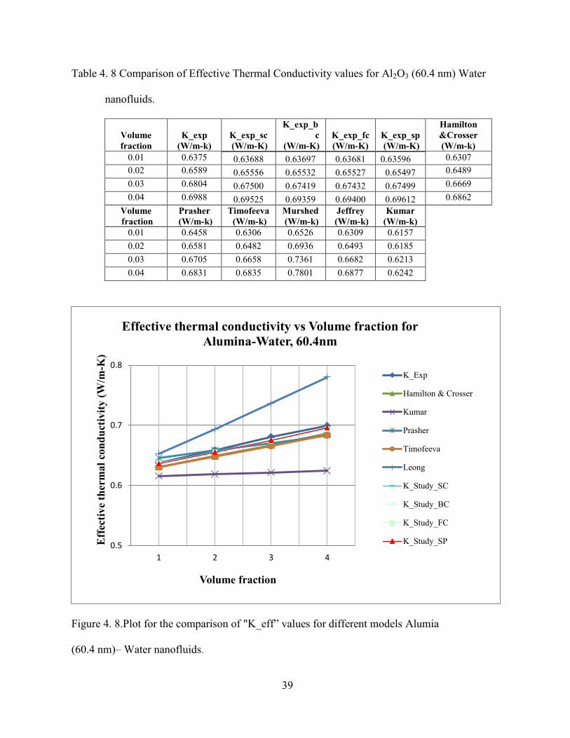
39

Table 4. 8 Comparison of Effective Thermal Conductivity values for Al2O3 (60.4 nm) Water

nanofluids.

Volume

fraction

K_exp

(W/m-k)

K_exp_sc

(W/m-K)

K_exp_b

c

(W/m-K)

K_exp_fc

(W/m-K)

K_exp_sp

(W/m-K)

Hamilton

&Crosser

(W/m-k)

0.01 0.6375 0.63688 0.63697 0.63681 0.63596 0.6307

0.02 0.6589 0.65556 0.65532 0.65527 0.65497 0.6489

0.03 0.6804 0.67500 0.67419 0.67432 0.67499 0.6669

0.04 0.6988 0.69525 0.69359 0.69400 0.69612 0.6862

Volume

fraction

Prasher

(W/m-k)

Timofeeva

(W/m-k)

Murshed

(W/m-k)

Jeffrey

(W/m-k)

Kumar

(W/m-k)

0.01 0.6458 0.6306 0.6526 0.6309 0.6157

0.02 0.6581 0.6482 0.6936 0.6493 0.6185

0.03 0.6705 0.6658 0.7361 0.6682 0.6213

0.04 0.6831 0.6835 0.7801 0.6877 0.6242

Figure 4. 8.P ot for the compar son of "K_eff” va ues for d fferent mode s Alumia

(60.4 nm)– Water nanofluids.

0.5

0.6

0.7

0.8

1 2 3 4

Eff

ecti

ve

ther

mal

con

du

ctiv

ity (

W/m

-K)

Volume fraction

Effective thermal conductivity vs Volume fraction for

Alumina-Water, 60.4nm

K_Exp

Hamilton & Crosser

Kumar

Prasher

Timofeeva

Leong

K_Study_SC

K_Study_BC

K_Study_FC

K_Study_SP

40

– EG 26 nm

The experimental data was collected from Feng et al. [40]. The experimental conditions

are identical to that described in Section 4.2. The parametric values used for prediction are:

p = 42.34 W/m-k, f . 5 W/m-k, Cp = 2145 J/kg k, f = 0.0157 N s m ,

f 1.5 1 -5 N s m , T = 300K,

f 111 . g m , tp 4.146 x -1 m.

To further validate the developed model,, it was used for the prediction of another

alumina-ethylene nanofluids wherein the diameter of nanoparticle is 26 nm. The effective

thermal conductivity values were estimated and the results are tabulated in Table 4.10 and

plotted as a function of volume fraction in Figure 4.9. Once again, the experimental values

coincide with the mathematical model values and slightly deviate at lower volume fractions

(Figure 4.9).

Table 4. 9. Volume fraction and mean diameter of cluster for Al2O3 (26 nm) – EG nanofluids.

Nanocluster

Simple

Cubic

Body

centered Face Centered Spherical

ɸc 0.4875 0.6056 0.6891 0.3793

p (nm) 32.2582 32.2582 71.4892 80.4877

41

Table 4. 10.Comparison of Effective Thermal Conductivity values for Al2O3 (26 nm)– EG

nanofluids.

Volume

fraction

K_exp

(W/m-k)

K_exp_sc

W/m-K)

K_exp_b

c

(W/m-K)

K_exp_fc

(W/m-K)

K_exp_sp

(W/m-K)

Hamilton

&Crosser

(W/m-k)

0.01 0.2625 0.27799 0.26784 0.27796 0.26701 0.2595

0.02 0.272 0.28590 0.27561 0.28577 0.27507 0.2682

0.03 0.2834 0.29417 0.28361 0.29386 0.28360 0.276

0.04 0.2909 0.30281 0.29186 0.30224 0.29265 0.284

Volume

fraction

Prasher

(W/m-k)

Timofeeva

(W/m-k)

Murshed

(W/m-k)

Jeffrey

(W/m-k)

Kumar

(W/m-k)

0.01 0.2745 0.2594 0.2676 0.2595 0.2612

0.02 0.2797 0.2669 0.2836 0.2673 0.2707

0.03 0.285 0.2743 0.3002 0.2753 0.2803

0.04 0.2904 0.2817 0.3173 0.2836 0.2898

Figure 4. 9. Plot for the comparison of "K_eff " values for different model

Al2O3 (26 nm)– EG 26 nanofluids.

0.25

0.26

0.27

0.28

0.29

0.3

0.31

0.32

0.33

1 2 3 4

Eff

ecti

ve

Th

erm

al

con

du

ctiv

ity (

W/m

-K)

Volume fraction

Effective thermal conductivity vs Volume fraction,

Alumima- water, 26 nm

K_exp

Hamilton & Crosser

Kumar

Prasher

Timofeeva

Leong

Jeffery

K_Study_SC

K_Study_BC

K_Study_FC

K_Study_SP

42

- Water 10 nm

The experimental data was collected from Kim et al. [49]. For the experiment, Kim et al.

[49] used transient hot - wire method with an anodized tantalum wire to measure the thermal

conductivity. A bare tantalum wire was electrically heated at an electrical potential of 50 v in

citric-acid solution to form an oxide layer on the surface. The hot wire was calibrated in a

constant temperature bath and the measured resistance was expressed in temperatures. Using

this temperature Kim et al. [49] calculated the thermal conductivity. The electric current was

adjusted to cause about 2 K temperature rise for 1 s. The voltage signal from the Wheatstone

bridge was amplified by approximately 1000 times and a digital Oscilloscope reads the signal at

a 2.5 kHz.

The parametric values used for model prediction in this case are as follows: p = 8.37

W/m-k, f W/m-k, Cp = 4170 J/kg k, f = 8.55× 1

-4 N s m , f 8.55 1

- N s m , T

= 300K, f g m , tp .844 x -1 m.

Table 4.12 summarizes the effective thermal conductivity of titanium-dioxide nanofluids

–both experimental and model predicted. The data is plotted as a function of volume fraction in

Figure 4.10. From the Figure 4.10 it is clear that the present model is better than the competing

models and is in concord with the experimental data. In addition, it is also observed that (Figure

4.10) the thermal conductivity values obtained by Prasher et al. [16] decreases with the increase

in the volume fraction of the nanoparticles which is in the contrast to the results that Prasher et

al. [37] got for other nanofluids. The results obtained from other models disagreed with the

experimental data. Up to now the effective thermal conductivity results were presented for

nanoparticle volume fractions 0.01, 0.02, 0.03 and 0.04. But in the case of Titanium oxide–

Water/EG and Zinc oxide– Water/EG nanofluids the results are presented only for 0.01, 0.02

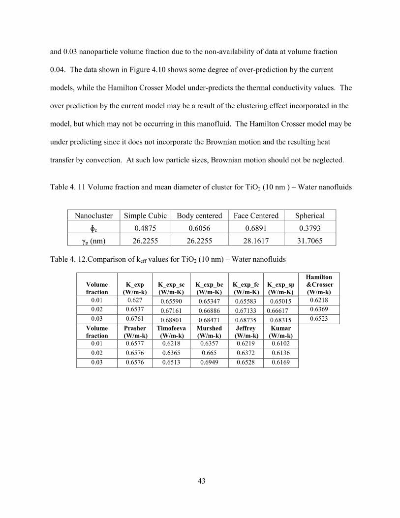
43

and 0.03 nanoparticle volume fraction due to the non-availability of data at volume fraction

0.04. The data shown in Figure 4.10 shows some degree of over-prediction by the current

models, while the Hamilton Crosser Model under-predicts the thermal conductivity values. The

over prediction by the current model may be a result of the clustering effect incorporated in the

model, but which may not be occurring in this manofluid. The Hamilton Crosser model may be

under predicting since it does not incorporate the Brownian motion and the resulting heat

transfer by convection. At such low particle sizes, Brownian motion should not be neglected.

Table 4. 11 Volume fraction and mean diameter of cluster for TiO2 (10 nm ) – Water nanofluids

Nanocluster Simple Cubic Body centered Face Centered Spherical

ɸc 0.4875 0.6056 0.6891 0.3793

p (nm) 26.2255 26.2255 28.1617 31.7065

Table 4. 12.Comparison of keff values for TiO2 (10 nm) – Water nanofluids

Volume

fraction

K_exp

(W/m-k)

K_exp_sc

(W/m-K)

K_exp_bc

(W/m-K)

K_exp_fc

(W/m-K)

K_exp_sp

(W/m-K)

Hamilton

&Crosser

(W/m-k)

0.01 0.627 0.65590 0.65347 0.65583 0.65015 0.6218

0.02 0.6537 0.67161 0.66886 0.67133 0.66617 0.6369

0.03 0.6761 0.68801 0.68471 0.68735 0.68315 0.6523

Volume

fraction

Prasher

(W/m-k)

Timofeeva

(W/m-k)

Murshed

(W/m-k)

Jeffrey

(W/m-k)

Kumar

(W/m-k)

0.01 0.6577 0.6218 0.6357 0.6219 0.6102

0.02 0.6576 0.6365 0.665 0.6372 0.6136

0.03 0.6576 0.6513 0.6949 0.6528 0.6169

44

Figure 4. 10. Plot for the comparison of "K_eff " values for different TiO2 (10 nm)–Water

nanofluids.

- Water 34 nm

The experimental data was collected from Kim et al. [49]. The experimental conditions

are identical as in the previous case. The parametric values used for the models are as follows:

p = 8.37 W/m-k, f W/m-k, Cp = 4170 J/kg k, f = 8.55× 1

-4 N s m ,

f 8.55 1 - N s m , T = 300K,

f g m , tp .844 x -1 m.

The thermal conductivity values were calculated for Titanium-oxide nanofluids and

provided in table 4.14. From the figure 4.11 it is seen distinctly that thermal conductivity values

are closer to the experimental data. The results from Jeffrey [46], Timofeeva et al. [44], Prasher

et al. [16] and

Hamilton & Crosser [32] lie closer to the experimental data at different cases, but the

0.58

0.6

0.62

0.64

0.66

0.68

0.7

1 2 3Eff

ecti

ve

Th

erm

al

Co

nd

uct

ivit

y (

W/m

-k)

Volume fraction


fraction, Titanium oxide - water, 10 nm

K_exp

Hamilton & Crosser

Kumar

Prasher

Timofeeva

Leong

Jeffrey

K_Study_SC

K_Study_BC

K_Study_FC

K_Study_SP

45

mathematical model displays better results in the entire range.

Table 4. 13 Volume fraction and mean diameter of cluster for TiO2 (34 nm)– Water nanofluids

Nanocluster

Simple

Cu

bic

Body

cente

red

Face

Cent

ered Spherical

ɸc 0.4875 0.6056 0.6891 0.3793

p (nm) 85.7791 85.7791 92.1121 103.7065

Table 4. 14 Comparison of Effective Thermal Conductivity values TiO2 (34 nm) – Water

nanofluids

Volume

fraction

K_exp

(W/m-k)

K_exp_sc

(W/m-K)

K_exp_bc

(W/m-K)

K_exp_fc

(W/m-K)

K_exp_sp

(W/m-K)

Hamilton

&Crosser

(W/m-k)

0.01 0.6239 0.6323 0.6315 0.6323 0.6306 0.6218 0.02 0.6452 0.6479 0.6468 0.6477 0.6465 0.6369 0.03 0.6598 0.6641 0.6625 0.6635 0.6632 0.6523

Volume

fraction

Prasher (

W/m-k)

Timofeeva

(W/m-k)

Murshed

(W/m-k)

Jeffrey

(W/m-k)

Kumar

(W/m-k)

0.01 0.6432 0.6218 0.6338 0.6219 0.608

0.02 0.6519 0.6365 0.6611 0.6372 0.6089

0.03 0.6607 0.6513 0.6888 0.6528 0.6099

46

Figure 4. 11 Plot for the comparison of K _eff values for different models TiO2 (33 nm) – Water

nanofluids

- Water 27 nm

The experimental data was collected from Xuan et al. [31]. The parametric values used for

0.56

0.58

0.6

0.62

0.64

0.66

0.68

0.7

1 2 3

Eff

ecti

ve

Th

erm

al

Co

nd

uct

ivit

y

(W/m

-K)

Volume Fraction


Fraction for Titanium Oxide-water, 34 nm

K_exp

Hamilton & Crosse

Kumar

Prasher

Timofeeva

Leong

Jeffrey

K_Study_SC

K_Study_BC

K_Study_FC

K_Study_SP

47

model predictions are: p = 8.37 W/m-k, f W/m-k, Cp = 4170 J/kg k, f =

8.55× 1 -4 N s m , f 8.55 1

- N s m , T = 300K,

f g m ,

tp .844 x -1 m.

The third set of validations was conducted to verify the consistency of the present model

with the Titanium-oxide nanofluids. The results are tabulated in Table 4.16 and the data was

plotted as function of volume fraction in Figure 4.12. It is seen in Figure 4.12 that thermal

conductivity values are in excellent agreement with the experimental data. For this type of

nanofluids combination the Kumar et al. [44] model did not show any significant enhancement

which indicates the dominance of present model. The results from Hamilton & Crosser [32],

Prasher et al. [16] and Timofeeva et al. [25] were able to explain significant portion of the

enhancement but were not thorough enough to explain the unusual thermal conductivity of the

nanofluids observed during experimentation.

Table 4. 15 Volume fraction and mean diameter of cluster for TiO2 (27 nm) – water

nanofluids

Nanocluster

Simple

Cubic

Body

centered

Face

Centered Spherical

ɸc 0.4875 0.6056 0.6891 0.3793

p (nm) 68.4093 68.4093 73.4599 82.7065

48

Table 4. 16 Comparison of Effective Thermal Conductivity values for TiO2 (27 nm) – water

nanofluids

Volume

fraction

K_exp

(W/m-k)

K_exp_sc

(W/m-K)

K_exp_bc

(W/m-K)

K_exp_fc

(W/m-K)

K_exp_sp

(W/m-K)

Hamilton

&Crosser

(W/m-k)

0.01 0.6314 0.64124 0.64025 0.64118 0.63907 0.628

0.02 0.6498 0.65697 0.65569 0.65671 0.65508 0.6432

0.03 0.6651 0.67330 0.67153 0.67272 0.67192 0.6587

Volume

fraction

Prasher

(W/m-k)

Timofeeva

(W/m-k)

Murshed

(W/m-k)

Jeffrey

(W/m-k)

Kumar

(W/m-k)

0.01 0.651 0.6279 0.6402 0.628 0.6142

0.02 0.6581 0.6427 0.6678 0.6434 0.6154

0.03 0.6653 0.6576 0.6959 0.6592 0.6167

Figure 4. 12 Plot for the comparison of "K_eff " values for different models TiO2 (27 nm) –

Water nanofluids

0.56

0.58

0.6

0.62

0.64

0.66

0.68

0.7

0.72

1 2 3

Eff

ecti

ve

Th

erm

al

Con

du

ctiv

ity

(W/m

-K)

Volume Fraction



K_exp

Hamilton & Crosse

Kumar

Prasher

Timofeeva

Leong

Jeffrey

K_Study_SC

K_Study_BC

K_Study_FC

K_Study_SP

49

- EG 34 nm

The experimental data was collected from Kim et al. [49]. The experimental procedures

are identical to that described in Section 4.6. The parametric values used for predicting thermal

conductivities are as follows: p = 8.37 W/m-k, f . 5 W/m-k, Cp = 2145 J/kg k, f =

0.0157 N s m , f 1.5 1 -5 N s m , T = 300K,

f 111 . g m , tp 4.146 x -1 m. The

developed model (for all cluster structures) was tested for Titanium oxide – Ethylene Glycol.

The results are shown in Table 4.18 and plotted in Figure 4.13. As seen from the figure 4.13, it

is once again shown that the model developed in this thesis explains the conductivity

enhancement in nanofluids more comprehensively than competing models. As observed earlier,

the results predicted by Prasher et al. [16] and Leong et al. [45] models overestimated the

experimental data whereas the other models underestimated the data.

Table 4. 17 Volume fraction and mean diameter of cluster for TiO2 (34 nm) - EG 34 nanofluids

Nanocluster

Simple

Cu

bic

Body

cente

red

Face

Cent

ered Spherical

ɸc 0.4875 0.6056 0.6891 0.3793

p (nm) 86.4253 86.4253 92.8060 104.4877

50

Table 4. 18 Comparison of Effective Thermal Conductivity values for TiO2 (34 nm) - EG 34

nanofluids

Figure 4. 13 P ot for the compar son of "K_eff” va ues for d fferent mode s

TiO2 (34 nm) - EG 34 nanofluids

0.24

0.25

0.26

0.27

0.28

0.29

0.3

1 2 3Eff

ecti

ve

ther

mal

con

du

ctiv

ity (

W/m

-K)

Volume fraction

Effective thermal conductivity vs volume

fraction, Titanium oxide, EG 34 nm

K_exp

Hamilton & Crosser

Kumar

Prasher

Timofeeva

Leong

Jeffrey

K_Study_SC

K_Study_BC

K_Study_FC

K_Study_SP

Volume

fraction

K_exp

(W/m-k)

K_exp_sc

(W/m-K)

K_exp_bc

(W/m-K)

K_exp_fc

(W/m-K)

K_exp_sp

(W/m-K)

Hamilton

&Crosser

(W/m-k)

0.01 0.261 0.26593 0.26541 0.26590 0.26478 0.2589

0.02 0.2719 0.27327 0.27262 0.27315 0.27226 0.267

0.03 0.2829 0.28092 0.28003 0.28064 0.28015 0.2733

Volume

fraction

Prasher

(W/m-k)

Timofeeva

(W/m-k)

Murshed

(W/m-k)

Jeffrey

(W/m-k)

Kumar

(W/m-k)

0.01 0.2734 0.2599 0.2664 0.26 0.2544

0.02 0.2782 0.2669 0.28 0.2673 0.2558

0.03 0.2831 0.2738 0.2939 0.2747 0.2573

51

ZnO – Water 10 nm

The experimental data was collected from Kim et al. [49]. The experimental procedure

is identical to that described in Section 4.6. The modeling parameters used are: p = 29 W/m-

k, f W/m-k, Cp = 4170 J/kg k, f = 8.55× 1

-4 N s m , f 8.55 1

- N s m , T =

300K, f g m , tp .884 x -1 m.

Here the study investigated the validity of the model for ZnO – Water nanofluids. So far

no previous models have shown their validation against ZnO - Water or Ethylene Glycol

nanofluids. The present study has shown some good results for ZnO in Water or Ethylene

Glycol. The values are calculated and tabulated in Table 4.20. Figure 4.14 shows that the

thermal conductivity agreement with the experimental data at higher volume fraction and at

lower fraction the mathematical model predicted values are slightly higher than the

experimental data. The deviation may be a result of the fact that the clustering is either too low

or thus single particle cases need to be considered. The trend seems to be similar to the

previous case of 10 nm nanoparticle based nanofluids.

Table 4. 19 Volume fraction and mean diameter of cluster for ZnO (10 nm) -Water nanofluids

Nanocluster

Simple

Cu

bic

Body

cente

red

Face

Cent

ered Spherical

ɸc 0.4875 0.6056 0.6891 0.3793

p (nm) 26.2255 26.2255 28.1617 31.7065

52

Table 4. 20 Comparison of Effective Thermal Conductivity values for ZnO (10 nm) -Water

nanofluids

Figure 4. 14 Plot for the comparison of "K_eff " values for different models ZnO-water 10 nm

0.56

0.58

0.6

0.62

0.64

0.66

0.68

0.7

0.72

0.74

1 2 3

Eff

ecti

ve

Th

erm

al

Con

du

ctiv

ity

(W/m

-K)

Volume Fraction


Fraction for ZnO-water, 10 nm

K_exp

Hamilton &Crosser

Kumar

Prasher

Timofeeva

Murshed

Jeffrey

K_Study_SC

K_Study_BC

K_Study_FC

K_Study_SP

Volume

fraction

K_exp

(W/m-k)

K_exp_sc

(W/m-K)

K_exp_bc

(W/m-K)

K_exp_fc

(W/m-K)

K_exp_sp

(W/m-K)

Hamilton &

Crosser

(W/m-k)

0.01 0.6367 0.65833 0.65589 0.65825 0.65260 0.6242

0.02 0.6652 0.67663 0.67382 0.67631 0.67127 0.6419

0.03 0.6931 0.69579 0.69232 0.69503 0.69110 0.6579

Volume

fraction

Prasher

(W/m-k)

Timofeeva

(W/m-k)

Murshed

(W/m-k)

Jeffrey

(W/m-k)

Kumar

(W/m-k)

0.01 0.6637 0.6303 0.6482 0.6305 0.6242

0.02 0.6635 0.6475 0.6843 0.6486 0.6357

0.03 0.6634 0.6648 0.7215 0.6671 0.6474

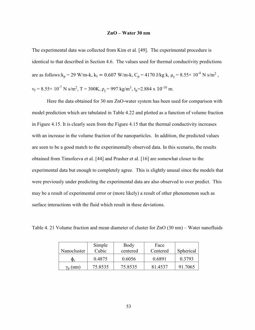
53

ZnO – Water 30 nm

The experimental data was collected from Kim et al. [49]. The experimental procedure is

identical to that described in Section 4.6. The values used for thermal conductivity predictions

are as follows: p = 29 W/m-k, f W/m-k, Cp = 4170 J/kg k, f = 8.55× 1

-4 N s m ,

f 8.55 1 - N s m , T = 300K,

f g m , tp .884 x -1 m.

Here the data obtained for 30 nm ZnO-water system has been used for comparison with

model prediction which are tabulated in Table 4.22 and plotted as a function of volume fraction

in Figure 4.15. It is clearly seen from the Figure 4.15 that the thermal conductivity increases

with an increase in the volume fraction of the nanoparticles. In addition, the predicted values

are seen to be a good match to the experimentally observed data. In this scenario, the results

obtained from Timofeeva et al. [44] and Prasher et al. [16] are somewhat closer to the

experimental data but enough to completely agree. This is slightly unusal since the models that

were previously under predicting the experimental data are also observed to over predict. This

may be a result of experimental error or (more likely) a result of other phenomenon such as

surface interactions with the fluid which result in these deviations.

Table 4. 21 Volume fraction and mean diameter of cluster for ZnO (30 nm) – Water nanofluids

Nanocluster

Simple

Cubic

Body

centered

Face

Centered Spherical

ɸc 0.4875 0.6056 0.6891 0.3793

p (nm) 75.8535 75.8535 81.4537 91.7065

54

Table 4. 22 Comparison of Effective Thermal Conductivity values for ZnO (30 nm) – Water

nanofluids

Volume

fraction

K_exp

(W/m-k)

K_exp_sc

(W/m-K)

K_exp_bc

(W/m-K)

K_exp_fc

(W/m-K)

K_exp_sp

(W/m-K)

Hamilton &

Crosser

(W/m-k)

0.01 0.627 0.63615 0.63524 0.63608 0.63423 0.6242

0.02 0.65 0.65432 0.65308 0.65403 0.65273 0.6419

0.03 0.6768 0.67324 0.67143 0.67257 0.67224 0.6598

Volume

fraction

Prasher

(W/m-k)

Timofeeva

(W/m-k)

Murshed

(W/m-k)

Jeffrey

(W/m-k)

Kumar

(W/m-k)

0.01 0.6501 0.6303 0.6468 0.6305 0.6167

0.02 0.658 0.6475 0.6814 0.6486 0.6206

0.03 0.666 0.6648 0.7166 0.6671 0.6245

Figure 4. 15 Plot for the comparison of "K_eff " values for different models

ZnO (30 nm) – Water nanofluids

0.58

0.6

0.62

0.64

0.66

0.68

0.7

0.72

0.74

0.01 0.02 0.03

Eff

ecti

ve

ther

nal

con

du

ctiv

ity (

W/m

-K)

Volume fraction

Effective thermal conductivity vs Volume

fraction, ZnO- Water 30 nm

K_exp

Hamilton & Crosser

Kumar

Prasher

Timofeeva

Leong

Jeffery

K_Study_SC

K_Study_BC

K_Study_FC

K_Study_SP

55

ZnO – EG 60 nm

The experimental data was collected from Kim et al. [49]. The experimental conditions

are identical to that described in Section 4.6. The nanofluids characteristic values used for the

model predictions are: p = 29 W/m-k, f . 5 W/m-k Cp = 2145 J/kg k, f = 0.0157 N s m ,

f 1.5 1 -5 N s m , T = 300K,

f 111 . g m , tp 4.146 x -1 m.

The present model was also validated for ZnO-EG nanofluids. Table 4.24 epitomizes the

thermal conductivity values for different volume fractions. This time also the model completely

agreed with the experimental data. The results are plotted as shown in the figure 4.16. The

other model predations followed the same pattern as that observed for previous nanofluids. For

ZnO-Water/EG nanofluids Prasher et al. [16], Timofeeva et al. [44], Hamilton & Crosser [32]

and Jeffrey [46] models performed significantly well but not the predictions were not as close as

that obtained from the current model

Table 4. 23 Volume fraction and mean diameter of cluster for ZnO (60 nm) – EG

nanofluids

Nanocluster

Simple

Cubic

Body

centered

Face

Centered Spherical

ɸc 0.4875 0.6056 0.6891 0.3793

p (nm) 150.9418 150.9418 162.0856 182.4877

56

Table 4. 24 Comparison of Effective Thermal Conductivity values for ZnO (60 nm) – EG

nanofluids

Volume

fraction

K_exp

(W/m-k)

K_exp_sc

(W/m-K)

K_exp_bc

(W/m-K)

K_exp_fc

(W/m-K)

K_exp_sp

(W/m-K)

Hamilton &

Crosser

(W/m-k)

0.01 0.2601 0.26345 0.26313 0.26342 0.26281 0.2594

0.02 0.2699 0.27127 0.27081 0.27115 0.27077 0.267

0.03 0.279 0.27942 0.27872 0.27913 0.27917 0.2747

Volume

fraction

Prasher

(W/m-k)

Timofeeva

(W/m-k)

Murshed

(W/m-k)

Jeffrey

(W/m-k)

Kumar

(W/m-k)

0.01 0.2693 0.2594 0.2667 0.2595 0.2547

0.02 0.2752 0.2667 0.2816 0.2672 0.2575

0.03 0.2813 0.2741 0.2969 0.2751 0.2604


ZnO (60 nm) – EG nanofluids

0.23

0.24

0.25

0.26

0.27

0.28

0.29

0.3

0.31

0.01 0.02 0.03

Eff

ecti

ve

ther

na

l co

nd

uct

ivit

y (

W/m

-K)

Volume fraction


fraction, ZnO-EG, 60 nm

K_exp

Hamilton & Crosser

Kumar

Prasher

Tmofeeva

Leong

Jeffrey

K_Study_SC

K_Study_BC

K_Study_FC

K_Study_SP

57

Cu-Water 100 nm

The experimental data was collected from Xuan et al. [31]. The nanofluids parameters

used for the model predictions are as follow: p = 401 W/m-k, f W/m-k, Cp = 4170

J/kg k, f = 8.55× 1

-4 N s m , f 8.55 1

- N s m , T = 300K,

f g m ,

tp .844 x -1 m.

The thermal conductivity values are calculated sign the various models and tabulated in

Table 4.26. It is seen in Figure 4.17 that the developed model does not model the 100nm Cu-

Water nanofluids system. The reason may be due to the larger diameter of the nanoparticles. Till

date there is no procedure for accurate calculation of the nanolayer thickness and the previous

investigators arbitrarily chose the nanolayer thickness without proof. As stated by Tillman [51]

the nanolayer thickness is dependent on the diameter of the nanoparticles. From the figure 4.13

it is visible that the present model does not match with experimental data except the Leong et al.

[45] model but it overestimated the experimental data.

Table 4. 25 Volume fraction and mean diameter of cluster for Cu (100 nm) – Water nanofluids

Nanocluster

Simple

Cubic

Body

centered

Face

Centered Spherical

ɸc 0.4875 0.6056 0.6891 0.3793

p (nm) 249.5517 249.5517 267.9757 301.7065

58

Table 4. 26 Comparison of Effective Thermal Conductivity values for Cu (100 nm) – Water

nanofluids

Volume

fraction

K_exp

(W/m-k)

K_exp_sc

(W/m-K)

K_exp_bc

(W/m-K)

K_exp_fc

(W/m-K)

K_exp_sp

(W/m-K)

Hamilton

&Crosser

(W/m-k)

0.01 0.6559 0.63526 0.63490 0.63519 0.63474 0.6315

0.02 0.711 0.65468 0.65399 0.65438 0.65450 0.6504

0.03 0.7539 0.67490 0.67361 0.67420 0.67533 0.6696

0.04 0.8091 0.69597 0.69381 0.69468 0.69730 0.6893

Volume

fraction

Prasher

(W/m-k)

Timofeeva

(W/m-k)

Murshed

(W/m-k)

Jeffrey

(W/m-k)

Kumar

(W/m-k)

0.01 0.6435 0.6313 0.6664 0.6316 0.6286

0.02 0.6581 0.6496 0.7219 0.6508 0.6444

0.03 0.6729 0.6679 0.7795 0.6705 0.6606

0.04 0.688 0.6862 0.8395 0.6909 0.6772


Cu (100 nm) – Water nanofluids

0.6

0.65

0.7

0.75

0.8

0.85

0.9

0.01 0.02 0.03 0.04

Eff

ecti

ve

Th

erm

al

Con

du

ctiv

ity

(W/m

-K)

Volume Fraction


Fraction for Cu-water, 100 nm

K_exp

Hamilton & Crosser

Kumar

Prasher

Timofeeva

Jeffrey

Leong

K_Study_SC

K_Study_BC

K_Study_FC

K_Study_SP

59

Al-Water 20 nm

The experimental data was collected from Xuan et al. [31]. The model parameters are:

p = 237 W/m-k, f W/m-k, Cp = 4170 J/kg k, f = 8.55× 1

-4 N s m ,

f 8.55 1 - N s m , T = 300K,

f g m , tp .844 x -1 m.

The developed model was also validated for Al-Water nanofluids. The results are

calculated and tabulated in Table 4.28 also It is seen in Figure 4.18 that the present model is in

excellent agreement with the experimental data. The other models repeated the same trends in

over prediction and underestimation as observed earlier. An interesting phenomenon was

observed from Kumar et al. [39] model. Up to this point the results predicted by the model

developed by Kumar was always under predicting the experimental data. However, in this

system it overestimated not only experimental data but also all other models. The study could

not figure any conclusions from this eccentric behavior of the Kumar et al. [39] model.

Table 4. 27 Volume fraction and mean diameter of cluster for Al (20 nm) – Water

nanofluids

Nanocluster Simple Cubic

Body

centered

Face

Centered Spherical

ɸc 0.4875 0.6056 0.6891 0.3793

p (nm) 51.0395 51.0395 54.8077 61.7065

60

Table 4. 28 Comparison of Effective Thermal Conductivity values for Al (20 nm) – Water

nanofluids

Volume

fraction

K_exp

(W/m-k)

K_exp_sc

(W/m-K)

K_exp_bc

(W/m-K)

K_exp_fc

(W/m-K)

K_exp_sp

(W/m-K)

Hamilton

&Crosser

(W/m-k)

0.01 0.6345 0.64919 0.64787 0.64911 0.64604 0.6314

0.02 0.659 0.66863 0.66694 0.66831 0.66512 0.6502

0.03 0.6878 0.68892 0.68660 0.68818 0.68478 0.6694

0.04 0.7049 0.71014 0.70687 0.70876 0.70505 0.689

Volume

fraction

Prasher

(W/m-k)

Timofeeva

(W/m-k)

Murshed

(W/m-k)

Jeffrey

(W/m-k)

Kumar

(W/m-k)

0.01 0.6538 0.6312 0.6529 0.6315 0.659

0.02 0.6587 0.6495 0.6941 0.6506 0.7059

0.03 0.6637 0.6677 0.7369 0.6703 0.7537

0.04 0.6686 0.686 0.7811 0.6906 0.8026

Figure 4. 18 Plot for the comparison of "K_eff " values for different model

Al (20 nm) – Water nanofluids

0.6

0.65

0.7

0.75

0.8

0.85

0.01 0.02 0.03 0.04Eff

ecti

ve

ther

mn

al

con

du

ctiv

ity (

W/m

K)

Volume fractioin


fraction, Al - Water, 20 nm

K_exp

Hamilton & Crosser

[20]Kumar [26]

Prasher [11]

Timofeeva [18]

Leong [27]

Jeffrey [28]

K_Study_SC

61

Fe-EG 10nm

The experimental data was taken from Hong and Yang [50]. For the experiment, Hong

and Yang [50] used transient hot wire method for calculating thermal conductivity of

nanofluids. The experiment procedure is the same as that of Eastman et al. [48] except that the

wire used was Teflon-coated pure platinum wire. The model parameters used are: p = 80.4

W/m-k, f . 5 W/m-k, Cp = 2145 J/kg k, f = 0.0157 N s m , f 1.5 1

-5 N s m , T =

300K, f 111 . g m , tp .844 x -1 m.

The model predictions are shown in figure 4.19. At the first glance the model does not

seem to model the nanofluids system well. However a closer scrutiny showed some interesting

information. This time the Prasher et al. [16] model and Kumar et al. [39] model prediction

were is close agreement to the experimental data, when compared to the developed model. In all

the cases discussed thus far in the thesis, the model by Leong et al. [45] overestimated the

thermal conductivities but in this case it underestimated the experimental data. So this

hypothesized that a very low volume fraction may be responsible for the disagreement of the

results. In addition, the thermal conductivity values of nanofluids are measured after sonicating

the nanofluids for 70 mins. After sonicating, the thermal conductivity was increased to 6.5% for

the volume fractions given below [50]. This directly indicates that the solids dispersion was not

efficient in the beginning and a good dispersion may yield better thermal conductivites –closer

to the predicted values.

62

Table 4. 29 Volume fraction and mean diameter of cluster for Fe (10 nm) – Water nanofluids

Nanocluster

Simple

Cu

bic Body centered

Face

Cent

ered Spherical

ɸc 0.4875 0.6056 0.6891 0.3793

p (nm) 26.2255 26.2255 28.1617 31.7065

Table 4. 30 Comparison of Effective Thermal Conductivity values for Fe (10 nm) – Water

nanofluids

Volume

fraction

K_exp

(W/m-K)

K_exp_sc

(W/m-K)

K_exp_bc

(W/m-K)

K_exp_fc

(W/m-K)

K_exp_sp

(W/m-K)

Hamilton &

Crosser

(W/m-K)

0.002 0.2693 0.27479 0.27377 0.27476 0.27241 0.2545

0.003 0.2758 0.28284 0.28166 0.28270 0.28062 0.2552

0.004 0.2779 0.29129 0.28981 0.29095 0.28936 0.256

0.0055 0.2802 0.30014 0.29824 0.29952 0.29867 0.2571

Volume

Fraction

Prasher

(W/m-K)

Timofeeva

(W/m-K)

Leong

(W/m-K)

Jeffrey

(W/m-K)

Kumar

(W/m-K)

0.002 0.2811 0.2515 0.2529 0.2545 0.262

0.003 0.2812 0.2522 0.2543 0.2553 0.2666

0.004 0.2814 0.253 0.2558 0.256 0.2711

0.0055 0.2815 0.2541 0.258 0.2572 0.2779

63


Fe-EG 10 nm

The above mentioned experimental thermal conductivities at all volume fractions are

decreased by about 6.5 % and tabulated in Table 4.15. The reason for the decrease is that the

values were measured after sonicating the nanofluid for 70 min. Now the calculated values

represent the natural thermal conductivity of the nanofluids. The new results were plotted in

Figure 4.6. As seen from Figure the present model has shown a decent behavior by getting

closer to experimental data. Previously predictions by Prasher et al. [16] model were a better,

match to experimental data but now it overestimated the experimental data. Also looking

closely, as the volume fraction of nanoparticles increased, no enhancement of thermal

conductivity values was predicted by the Prasher et al. [16] model. This is in contrast to theory

0.22

0.23

0.24

0.25

0.26

0.27

0.28

0.29

0.3

0.31

0.002 0.003 0.004 0.0055

Eff

ecti

ve

ther

mal

con

du

ctiv

ity (

W/m

k)

Volume fraction


Fraction for Fe-EG, 10 nm

K_exp

Hamilton &

CrosserKumar

Prasher

Timofeeva

64

because the thermal conductivity should increase when concentration of nanoparticles are

increased. So far Kumar et al. [39] model did not explain the unusual behavior of nanofluids.

But as seen from Figure 4.2 it is the only model that successfully agreed to the experimental

data. This shows that Kumar et al. [39] model is not consistent but may have some

characteristic that is worth investigating to improve the current model.

Conclusion

From the discussions above and all the graphs, the study concluded that the developed

model is more accurate than the other models. The model was validated for a wide range of

available nanofluid combinations. Previous studies by many researchers did not include the

results as depicted in the present study. The value of the constant C = 0.7*Pr is used for all

Water and Ethylene Glycol based nanofluids. The thermal conductivity of the nanofluids

increased with increase in volume fraction of the nanoparticles. The model is in good agreement

with experimental data for almost all the nanofluids except for Cu –water and Fe – EG. The

reasons for the discrepancy were explained in their respective sections (4.13 and 4.15). The

assumptions and estimation of possible critical factors for explaining the thermal conductivity

of nanofluids is justified.

The predictions from four cluster models are in good agreement with the experimental

values. The spherical cluster is the one which has the least deviation from the experimental

values. Hence we assume that the analyzed nanofluids form a spherical cluster and the

Brownian motion and the nanolayer formed around the cluster, the volume fraction of the

cluster and the nanofluid trapped in the clusters helps to increase the thermal conductivity in

nanofluids.

65

CHAPTER 5

PARAMETRIC STUDY OF THE PROPERTIES OF NANOFLUIDS

The study has developed a mathematical model for thermal conductivity of nanofluids.

This chapter deals with issues that would help us understand the properties which affect the

thermal conductivity of nanofluids. The effect of volume fraction and nanoclustering effect on

thermal conductivity were seen in chapter 4, where the thermal conductivity increases linearly

with increase in the volume fraction of the nanoparticles. Three other factors such as nanolayer

thickness, diameter of the nanoparticles and effect of Brownian motion are also considered for

study. The results are determined by varying one factor while keeping others constant.

A. Effect of Nanolayer thickness on the overall thermal conductivity of nanofluids:

The nanolayer thickness was considered as a critical parameter for thermal conductivity

enhancement. The nanolayer thickness values for water and Ethylene Glycol was calculated.

The nanolayer thickness for water as a base fluid was found to be 0.2884 nm. The values of the

nanolayer thickness were varied from 0.01 nm to 1 nm in case of water used as a base fluid. In

case of Ethylene Glycol, the nanolayer thickness was found to be 0.414 nm. The thickness was

varied from 0.2 to 1 nm to carry out the parametric study. The volume fraction was varied from

0.01 to 0.04. Spherical clusters was considered for the thermal conductivity calculations. The

values of thermal conductivity were calculated for various nanofluids and the graphs are plotted

and are shown below.

66

CuO – Water / EG

Table 5. 1 Variation of effective thermal conductivity with nanolayer thickness

CuO (18 nm) - Water nanofluids

Nanolayer Thickness

(nm)

Volume Fraction

0.01 0.02 0.03 0.04

0.01 0.6485 0.66656 0.68555 0.70553

0.05 0.64842 0.6665 0.68552 0.70556

0.1 0.64833 0.66643 0.6855 0.7056

0.2 0.64815 0.6663 0.68545 0.70568

0.2884 0.648 0.66619 0.68542 0.70576

0.3 0.64797 0.66617 0.68541 0.70578

0.4 0.6478 0.66605 0.68538 0.70589

0.6 0.64746 0.66582 0.68534 0.70614

0.8 0.64715 0.66562 0.68534 0.70645

1 0.64685 0.66543 0.68537 0.70681

Figure 5. 1 Effective thermal conductivity versus the nanolayer thickness for CuO (18 nm) -

Water nanofluids

0.64

0.65

0.66

0.67

0.68

0.69

0.7

0.71

0 0.5 1 1.5

K_ef

f (W

/m-K

)

Nanolayer Thickness (nm)

K_eff for CuO - Water 18 nm

0.01

0.02

0.03

0.04

67

Table 5. 2 Variation of effective thermal conductivity with nanolayer thickness CuO

(23.6 nm) - Water nanofluids

Nanolayer Volume fraction

thickness

(nm) 0.01 0.02 0.03 0.04

0.01 0.6442 0.6622 0.6812 0.7012

0.05 0.6441 0.6622 0.6812 0.7012

0.1 0.6441 0.6622 0.6812 0.7013

0.2 0.6440 0.6621 0.6812 0.7014

0.2884 0.6440 0.6621 0.6812 0.7014

0.3 0.6439 0.6620 0.6812 0.7015

0.4 0.6438 0.6620 0.6812 0.7016

0.6 0.6436 0.6618 0.6812 0.7018

0.8 0.6434 0.6617 0.6813 0.7021

1 0.6432 0.6616 0.6813 0.7024

Figure 5. 2 Effective thermal conductivity versus the nanolayer thickness for CuO

(23.6 nm) - Water nanofluids

0.6400

0.6500

0.6600

0.6700

0.6800

0.6900

0.7000

0.7100

0 0.5 1 1.5

K_ef

f (W

/m-K

)


K_eff for CuO - Water 23.6 nm

0.01

0.02

0.03

0.04

68

CuO – EG 30.8 nm

Table 5. 3. Variation of effective thermal conductivity with nanolayer thickness CuO (30.8 nm)

– EG nanofluids

Nanolayer Volume Fraction

thickn

ess(n

m) 0.01 0.02 0.03 0.04

0.2 0.2659 0.2739 0.2823 0.2912

0.3 0.2659 0.2739 0.2823 0.2913

0.4 0.2659 0.2739 0.2823 0.2913

0.414 0.2658 0.2739 0.2823 0.2913

0.6 0.2658 0.2738 0.2823 0.2914

0.8 0.2657 0.2738 0.2823 0.2914

1 0.2656 0.2737 0.2823 0.2915

2 0.2653 0.2736 0.2825 0.2921

3 0.2651 0.2735 0.2827 0.2928

4 0.2649 0.2735 0.2831 0.2938

Figure 5. 3 Effective thermal conductivity versus the nanolayer thickness for

0.2600

0.2650

0.2700

0.2750

0.2800

0.2850

0.2900

0.2950

0.3000

0 1 2 3 4 5

K_

eff

(W/m

-K)


K_eff for CuO - EG 30.8 nm

0.01

0.02

0.03

0.04

69


The values are calculated and tabulated in table 5.1, 5.2, 5.3 and plotted in figures 5.1,

5.2 and 5.3. As seen from the figures, the effective thermal conductivity decreased with increase

in the nanolayer thickness except for higher volume fractions. The results suggest that nanolayer

formation is a crucial factor for the abnormal thermal conductivity of the nanofluids.

Al2O3– Water / EG

Table 5. 4 Variation of effective thermal conductivity with nanolayer thickness Al2O3 (60.4

nm) - Water nanofluids


thickness (nm) 0.0100 0.0200 0.0300 0.0400

0.01 0.6360 0.6550 0.6749 0.6959

0.05 0.6360 0.6550 0.6749 0.6960

0.1 0.6360 0.6550 0.6749 0.6960

0.2 0.6360 0.6550 0.6750 0.6961

0.288 0.6360 0.6550 0.6750 0.6961

0.3 0.6360 0.6550 0.6750 0.6961

0.4 0.6359 0.6550 0.6750 0.6962

0.6 0.6359 0.6550 0.6751 0.6963

0.8 0.6359 0.6550 0.6752 0.6965

1 0.6359 0.6550 0.6752 0.6966

70

Figure 5. 4 Effective thermal conductivity versus nanolayer thickness for Al2O3 (60.4 nm) -

Water nanofluids

Table 5. 5 Variation of effective thermal conductivity with nanolayer thickness Al2O3 (26

nm) – EG nanofluids


thickness

(nm) 0.01 0.02 0.03 0.04

0.2 0.2671 0.2751 0.2836 0.2926

0.3 0.2671 0.2751 0.2836 0.2926

0.4 0.2670 0.2751 0.2836 0.2926

0.414 0.2670 0.2751 0.2836 0.2926

0.6 0.2669 0.2750 0.2836 0.2927

0.8 0.2668 0.2749 0.2836 0.2928

1 0.2667 0.2749 0.2836 0.2929

2 0.2663 0.2747 0.2837 0.2936

3 0.2660 0.2745 0.2840 0.2945

4 0.2657 0.2745 0.2845 0.2959

0.6300

0.6400

0.6500

0.6600

0.6700

0.6800

0.6900

0.7000

0 0.5 1 1.5

K_ef

f (W

/m-K

)


K_eff for Al2O3 - Water 60.4 nm

0.01

0.02

0.03

0.04

71

Figure 5. 5 Effective thermal conductivity versus nanolayer thickness for Al2O3 (26 nm) – EG

nanofluids

Similar results are obtained as that of the above nanofluid. Figures 5.4 and 5.5 depict

that at constant volume fraction the thermal conductivity decreases with the increase in

nanolayer thickness. So the study came to conclusion that nanolayer is an important

contributing factor for overall thermal conductivity of the nanofluids.

0.2600

0.2650

0.2700

0.2750

0.2800

0.2850

0.2900

0.2950

0.3000

0 1 2 3 4 5

K_ef

f (W

/m-K

)


K_eff for Al2O3 - EG 26 nm

0.01

0.02

0.03

0.04

72

TiO2- Water / EG:

Table 5. 6 Variation of effective thermal conductivity with nanolayer thickness TiO2 (10

nm) – Water nanofluids


thickness

(nm) 0.0100 0.0200 0.0300 0.0400

0.01 0.6516 0.6674 0.6840 0.7014

0.05 0.6514 0.6672 0.6839 0.7014

0.1 0.6511 0.6670 0.6837 0.7013

0.2 0.6506 0.6665 0.6834 0.7012

0.288 0.6501 0.6662 0.6831 0.7012

0.3 0.6501 0.6661 0.6831 0.7011

0.4 0.6496 0.6657 0.6829 0.7011

0.6 0.6487 0.6650 0.6825 0.7013

0.8 0.6478 0.6643 0.6822 0.7016

1 0.6470 0.6637 0.6820 0.7021


TiO2 (10 nm) - Water nanofluids

0.6400

0.6500

0.6600

0.6700

0.6800

0.6900

0.7000

0.7100

0 0.5 1 1.5

K_ef

f (W

/m-K

)


K_eff for TiO2 - Water 10 nm

0.01

0.02

0.03

0.04

73




thickness

(nm) 0.0100 0.0200 0.0300 0.0400

0.01 0.6308 0.6466 0.6632 0.6806

0.05 0.6308 0.6466 0.6632 0.6806

0.1 0.6307 0.6466 0.6632 0.6806

0.2 0.6307 0.6466 0.6632 0.6807

0.288 0.6307 0.6465 0.6632 0.6808

0.3 0.6307 0.6465 0.6632 0.6808

0.4 0.6306 0.6465 0.6632 0.6809

0.6 0.6305 0.6465 0.6633 0.6811

0.8 0.6305 0.6464 0.6633 0.6812

1 0.6304 0.6464 0.6634 0.6814

Figure 5. 7 Effective thermal conductivity versus nanolayer thickness for


0.6200

0.6300

0.6400

0.6500

0.6600

0.6700

0.6800

0.6900

0 0.5 1 1.5

K_ef

f (W

/m-K

)



0.01

0.02

0.03

0.04

74




thickness

(nm) 0.0100 0.0200 0.0300 0.0400

0.01 0.6393 0.6552 0.6719 0.6895

0.05 0.6392 0.6552 0.6719 0.6895

0.1 0.6392 0.6552 0.6719 0.6895

0.2 0.6391 0.6551 0.6719 0.6896

0.288 0.6391 0.6551 0.6719 0.6897

0.3 0.6391 0.6551 0.6719 0.6897

0.4 0.6390 0.6550 0.6719 0.6898

0.6 0.6389 0.6550 0.6720 0.6900

0.8 0.6387 0.6549 0.6720 0.6902

1 0.6386 0.6548 0.6721 0.6904

Figure 5. 8 Effective thermal conductivity versus the nanolayer thickness for TiO2 (27 nm)

- Water nanolfuids

0.6300

0.6400

0.6500

0.6600

0.6700

0.6800

0.6900

0.7000

0 0.5 1 1.5

K_ef

f (W

/m-K

)



0.01

0.02

0.03

0.04

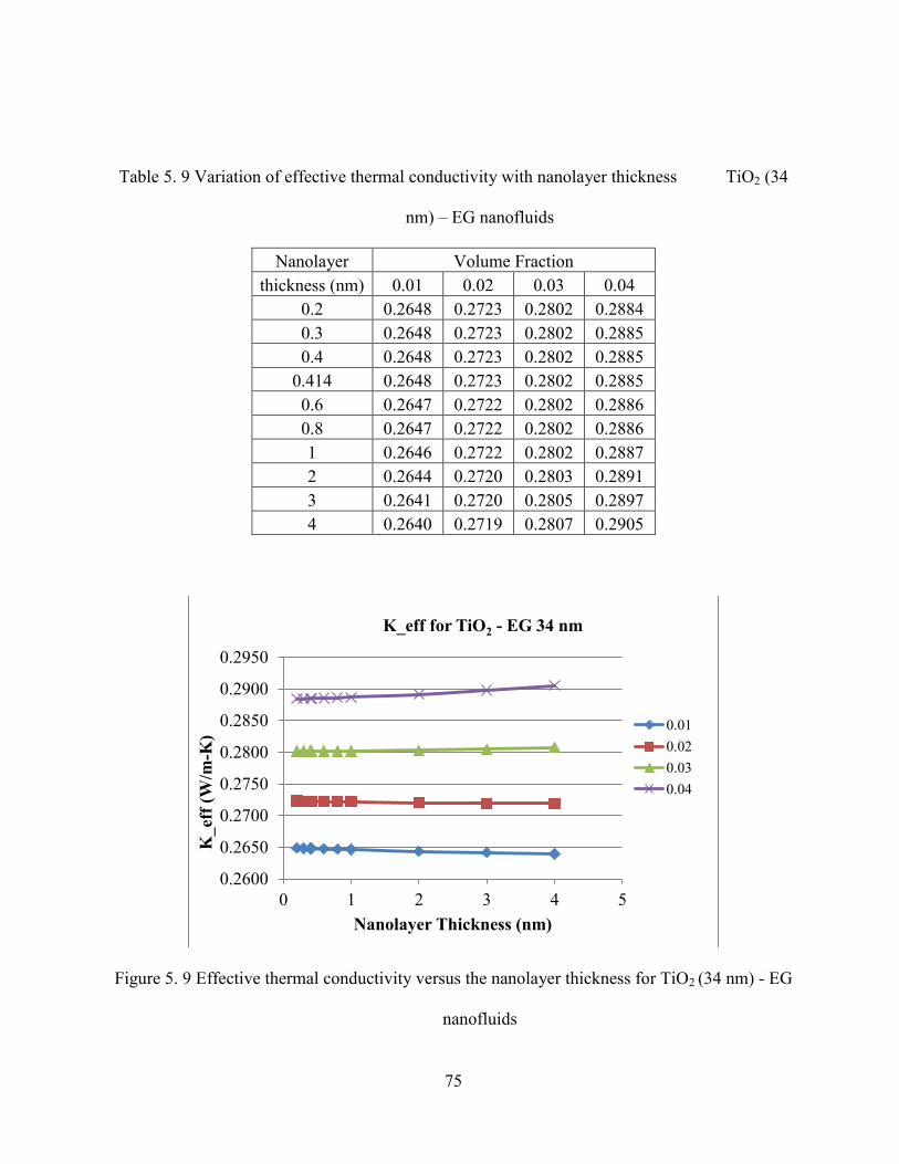
75




thickness (nm) 0.01 0.02 0.03 0.04

0.2 0.2648 0.2723 0.2802 0.2884

0.3 0.2648 0.2723 0.2802 0.2885

0.4 0.2648 0.2723 0.2802 0.2885

0.414 0.2648 0.2723 0.2802 0.2885

0.6 0.2647 0.2722 0.2802 0.2886

0.8 0.2647 0.2722 0.2802 0.2886

1 0.2646 0.2722 0.2802 0.2887

2 0.2644 0.2720 0.2803 0.2891

3 0.2641 0.2720 0.2805 0.2897

4 0.2640 0.2719 0.2807 0.2905

Figure 5. 9 Effective thermal conductivity versus the nanolayer thickness for TiO2 (34 nm) - EG

nanofluids

0.2600

0.2650

0.2700

0.2750

0.2800

0.2850

0.2900

0.2950

0 1 2 3 4 5

K_ef

f (W

/m-K

)


K_eff for TiO2 - EG 34 nm

0.01

0.02

0.03

0.04

76

The results followed the same trend as that of the previous nanofluids discussed above.

Again as seen from figures 5.6, 5.7, 5.8 and 5.9 the thermal conductivity of nanofluids

decreased with increase in the nanolayer thickness. This clearly shows the strong dependency of

nanolayer thickness on thermal conductivity of nanofluids.

ZnO – Water/EG:

Table 5. 10 Variation of effective thermal conductivity with nanolayer thickness ZnO (10



thickness (nm) 0.01 0.02 0.03 0.04

0.01 0.6541 0.6725 0.6919 0.7123

0.05 0.6538 0.6723 0.6917 0.7122

0.1 0.6536 0.6721 0.6916 0.7122

0.2 0.6530 0.6716 0.6913 0.7122

0.288 0.6526 0.6713 0.6911 0.7122

0.3 0.6525 0.6712 0.6911 0.7122

0.4 0.6520 0.6708 0.6909 0.7123

0.6 0.6511 0.6701 0.6906 0.7126

0.8 0.6503 0.6695 0.6904 0.7131

1 0.6495 0.6690 0.6903 0.7138

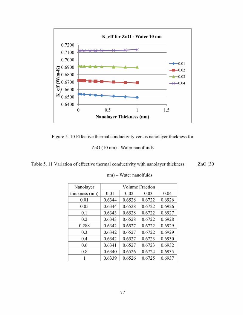
77

Figure 5. 10 Effective thermal conductivity versus nanolayer thickness for

ZnO (10 nm) - Water nanofluids


nm) – Water nanolfuids


thickness (nm) 0.01 0.02 0.03 0.04

0.01 0.6344 0.6528 0.6722 0.6926

0.05 0.6344 0.6528 0.6722 0.6926

0.1 0.6343 0.6528 0.6722 0.6927

0.2 0.6343 0.6528 0.6722 0.6928

0.288 0.6342 0.6527 0.6722 0.6929

0.3 0.6342 0.6527 0.6722 0.6929

0.4 0.6342 0.6527 0.6723 0.6930

0.6 0.6341 0.6527 0.6723 0.6932

0.8 0.6340 0.6526 0.6724 0.6935

1 0.6339 0.6526 0.6725 0.6937

0.6400

0.6500

0.6600

0.6700

0.6800

0.6900

0.7000

0.7100

0.7200

0 0.5 1 1.5

K_ef

f (W

/m-K

)


K_eff for ZnO - Water 10 nm

0.01

0.02

0.03

0.04

78


ZnO (30 nm) - Water nanofluids




thickness (nm) 0.01 0.02 0.03 0.04

0.2 0.2628 0.2708 0.2792 0.2880

0.3 0.2628 0.2708 0.2792 0.2880

0.4 0.2628 0.2708 0.2792 0.2880

0.414 0.2628 0.2708 0.2792 0.2880

0.6 0.2628 0.2708 0.2792 0.2881

0.8 0.2628 0.2708 0.2792 0.2881

1 0.2628 0.2708 0.2792 0.2882

2 0.2627 0.2707 0.2793 0.2885

3 0.2626 0.2708 0.2795 0.2889

4 0.2625 0.2708 0.2796 0.2892

0.6300

0.6400

0.6500

0.6600

0.6700

0.6800

0.6900

0.7000

0 0.5 1 1.5

K_ef

f (W

/m-K

)


K_eff for ZnO - Water 30 nm

0.01

0.02

0.03

0.04

79


ZnO (60 nm) - EG nanofluids

The results are similar for ZnO-Water/EG nanofluids also. From the table 5.10, 5.11,

5.12 and figures 5.10, 5.11 and 5.12 the study came to conclusion that nanolayer thickness is a

significant factor for unusual thermal conductivity of nanofluids.

0.2600

0.2650

0.2700

0.2750

0.2800

0.2850

0.2900

0.2950

0 2 4 6

K_ef

f (W

/m-K

)


K_eff for ZnO - EG 60 nm

0.01

0.02

0.03

0.04

80

Cu-Water/Al-Water/Fe-EG:

Table 5. 13 Variation of effective thermal conductivity with nanolayer thickness Al (20



thickness (nm) 0.01 0.02 0.03 0.04

0.01 0.6464 0.6654 0.6850 0.7051

0.05 0.6464 0.6654 0.6849 0.7051

0.1 0.6463 0.6653 0.6849 0.7051

0.2 0.6462 0.6652 0.6848 0.7050

0.288 0.6460 0.6651 0.6848 0.7050

0.3 0.6460 0.6651 0.6848 0.7050

0.4 0.6459 0.6650 0.6847 0.7051

0.6 0.6456 0.6648 0.6846 0.7051

0.8 0.6454 0.6646 0.6845 0.7051

1 0.6452 0.6644 0.6844 0.7052


Al (20 nm) – Water nanofluids

0.6400

0.6500

0.6600

0.6700

0.6800

0.6900

0.7000

0.7100

0 0.5 1 1.5

K_

eff

(W/m

-K)


K_eff for Al - Water 20 nm

0.01

0.02

0.03

0.04

81

Table 5. 14 Variation of effective thermal conductivity with nanolayer thickness Cu (100



thickness (nm) 0.01 0.02 0.03 0.04

0.01 0.6348 0.6545 0.6753 0.6972

0.05 0.6348 0.6545 0.6753 0.6972

0.1 0.6347 0.6545 0.6753 0.6972

0.2 0.6347 0.6545 0.6753 0.6973

0.288 0.6347 0.6545 0.6753 0.6973

0.3 0.6347 0.6545 0.6753 0.6973

0.4 0.6347 0.6545 0.6754 0.6974

0.6 0.6347 0.6545 0.6754 0.6975

0.8 0.6347 0.6545 0.6754 0.6976

1 0.6347 0.6545 0.6755 0.6977


Cu (100 nm) – Water nanofluids

0.6300

0.6400

0.6500

0.6600

0.6700

0.6800

0.6900

0.7000

0.7100

0 0.5 1 1.5

K_ef

f (W

/m-K

)


K_eff for Cu - Water 100 nm

0.01

0.02

0.03

0.04

82

Table 5. 15 Variation of effective thermal conductivity with nanolayer thickness Fe (10



Thickness

(nm) 0.01 0.02 0.03 0.04

0.2 0.2726 0.2808 0.2894 0.2986

0.3 0.2724 0.2806 0.2893 0.2987

0.4 0.2722 0.2804 0.2893 0.2987

0.414 0.2721 0.2804 0.2893 0.2987

0.6 0.2718 0.2802 0.2892 0.2989

0.8 0.2714 0.2799 0.2891 0.2991

1 0.2711 0.2797 0.2891 0.2995

2 0.2699 0.2792 0.2901 0.3029

3 0.2691 0.2795 0.2930 0.3110

4 0.2686 0.2809 0.2994 0.3302

Figure 5. 15 Effective thermal conductivity versus the nanolayer thickness

Fe (10 nm) – EG nanofluids

0.1000

0.1500

0.2000

0.2500

0.3000

0.3500

0 1 2 3 4 5

K_ef

f (W

/m-K

)


K_eff for Fe- EG 10 nm

0.

010.

020.

03

83

The results are replicated above but with some deviation. As seen from table 5.13 the

thermal conductivity of the nanofluid decreased with the increase in nanolayer thickness. Figure

5.14 the thermal conductivity remained almost constant for Cu-Water 100 nm nanofluid. This

might be because of the large nanoparticle diameter value. Figure 5.15 Fe – EG 10 nm, the

thermal conductivity increases at higher volume fractions with the increase in nanolayer

thickness, may be due to the smaller size of the nanoparticle.

Tillman et al. [51] also stated that an interfacial structure formed by liquid molecular

layering will play an important role. Feng et al. [40] also came to a conclusion that solid/liquid

interfacial layer is the pivotal factor for thermal conductivity of the nanofluids. Leong et al. [45]

proposed that nanolayer is one of the major mechanisms enhancing the thermal conductivity of

the nanofluids. From the above statements made by researchers, and all the graphs discussed so

far the study came to a conclusion that the nanolayer thickness is an important element in

enhancing the thermal conductivity of the nanofluids

B. Effect of particle diameter on effective thermal conductivity of nanofluids

The volume fraction and temperature were kept constant at 0.03 and 300k respectively.

These numbers were taken arbitrarily. The nanolayer thickness which was earlier used for

different nanofluid combinations in chapter 4 for model validation was used here too. All other

parameters were kept constant while varying the particle diameter. The particle diameter has

been varied from its average diameter in increments of 1 nm and decrements of 1nm for all

respective nanofluids. The values for the thermal conductivities were calculated and tabulated in

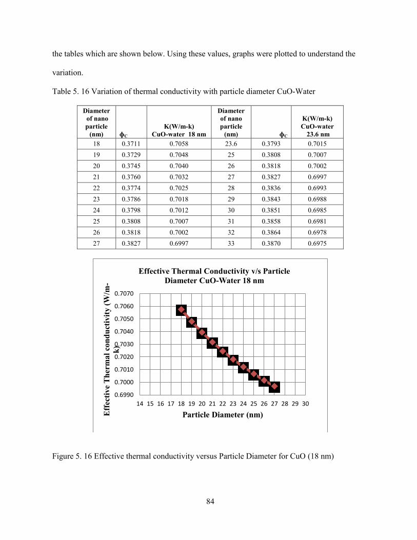
84

the tables which are shown below. Using these values, graphs were plotted to understand the

variation.

Table 5. 16 Variation of thermal conductivity with particle diameter CuO-Water

Diameter

of nano

particle

(nm) ɸC

K(W/m-k)

CuO-water 18 nm

Diameter

of nano

particle

(nm) ɸC

K(W/m-k)

CuO-water

23.6 nm

18 0.3711 0.7058 23.6 0.3793 0.7015

19 0.3729 0.7048 25 0.3808 0.7007

20 0.3745 0.7040 26 0.3818 0.7002

21 0.3760 0.7032 27 0.3827 0.6997

22 0.3774 0.7025 28 0.3836 0.6993

23 0.3786 0.7018 29 0.3843 0.6988

24 0.3798 0.7012 30 0.3851 0.6985

25 0.3808 0.7007 31 0.3858 0.6981

26 0.3818 0.7002 32 0.3864 0.6978

27 0.3827 0.6997 33 0.3870 0.6975

Figure 5. 16 Effective thermal conductivity versus Particle Diameter for CuO (18 nm)

0.6990

0.7000

0.7010

0.7020

0.7030

0.7040

0.7050

0.7060

0.7070

14 15 16 17 18 19 20 21 22 23 24 25 26 27 28 29 30

Eff

ecti

ve

Th

erm

al

con

du

ctiv

ity (

W/m

-

k)

Particle Diameter (nm)

Effective Thermal Conductivity v/s Particle

Diameter CuO-Water 18 nm

85

Figure 5. 17 Effective thermal conductivity versus Particle diameter for

CuO (23.6 nm)-Water

Table 5. 17 variation of thermal conductivity with particle diameter CuO - EG and Al2O3 -

Water

Diameter

of nano

particle

(nm) ɸC

K(W/m-k)

CuO-EG 30.8nm

Diameter of

nanoparticle

(nm) ɸC

K(W/m-k)

Al2O3-water

60.4 nm

30.8 0.3762 0.2913 60.4 0.3961 0.6961

32 0.3773 0.2911 62 0.3964 0.6960

33 0.3782 0.2909 63 0.3966 0.6959

34 0.3790 0.2907 64 0.3967 0.6958

35 0.3798 0.2905 65 0.3969 0.6958

36 0.3805 0.2904 66 0.3971 0.6957

37 0.3812 0.2902 67 0.3972 0.6956

38 0.3819 0.2901 68 0.3974 0.6956

39 0.3825 0.2899 69 0.3975 0.6955

40 0.3831 0.2898 70 0.3976 0.6954

0.6960

0.6980

0.7000

0.7020

20 21 22 23 24 25 26 27 28 29 30 31 32 33 34 35

Eff

ecti

ve

Th

erm

al

con

du

ctiv

ity

(W/m

-k)


Effective Thermal Conductivity v/s Particle Diameter

CuO-water 23.6 nm

86

Figure 5. 18 Effective thermal conductivity versus Particle diameter for CuO (30.8 nm)

Figure 5. 19 Effective thermal conductivity versus Particle diameter for Al2O3 (60.4 nm)

0.2890

0.2900

0.2910

0.2920

30 31 32 33 34 35 36 37 38 39 40

Eff

ecti

ve

Th

erm

al

con

du

ctiv

ity

(W/m

-k)



CuO-EG 30.8nm

0.6940

0.6960

0.6980

59 60 61 62 63 64 65 66 67 68 69 70 71

Eff

ecti

ve

Th

erm

al

con

du

ctiv

ity

(W/m

-k)



Al2O3-water 60.4 nm

87

As seen from the table 5.16 the diameter of the CuO-Water 18 nm has been varied from

18 nm to 27 nm with the increments of 1nm and for CuO-Water 23.6 nm the diameter has been

varied from 25 nm to 33 nm with an increment of 1nm. The increase in diameter increases the

cluster size. Spherical cluster formation has been assumed for this study. The values of thermal

conductivity were calculated and tabulated in table 5.16. It can be observed from the table 5.16

and figures 5.16 and 5.17 that at constant volume fraction, the thermal conductivity of the

nanofluid decreases as the particle diameter increases.

Also the diameter of CuO-EG 35 nm has been varied from 30 nm to 40 nm with an

increment of 1nm and for the Al2O3-Water 60.4 nm the particle diameter has been varied from

60 nm to 70 nm. The results were tabulated in table 5.17 and graphs were plotted. Similar

results were obtained as the above mentioned nanofluids. So the thermal conductivity of the

nanofluid decreases with the increase in the diameter of the nanoparticle.

Table 5. 18 Variation of thermal conductivity with particle diameter Al2O3-EG and TiO2 –

Water

Diameter

of nano

particle (nm) ɸC

K(W/m-k)

Al2O3-EG 26

nm

Diameter

of nano

particle

(nm) ɸC

K(W/m-k)

TiO2-Water

10 nm

26 0.3708 0.2926 10 0.3451 0.7012

27 0.3721 0.2924 11 0.3502 0.6986

28 0.3733 0.2921 12 0.3546 0.6965

29 0.3744 0.2919 13 0.3583 0.6946

30 0.3754 0.2916 14 0.3615 0.6931

31 0.3764 0.2914 15 0.3644 0.6917

32 0.3773 0.2912 16 0.3669 0.6905

33 0.3782 0.2910 17 0.3691 0.6894

34 0.3790 0.2909 18 0.3711 0.6885

35 0.3798 0.2907 19 0.3729 0.6876

88


Al2O3 (26 nm)


0.2905

0.2910

0.2915

0.2920

0.2925

0.2930

25 26 27 28 29 30 31 32 33 34 35 36 37

Eff

ecti

ve

Th

erm

al

con

du

ctiv

ity

(W/m

-k)



Diameter Al2O3-EG 26 nm

0.6860

0.6880

0.6900

0.6920

0.6940

0.6960

0.6980

0.7000

0.7020

8 9 10 11 12 13 14 15 16 17 18 19 20 21 22

Eff

ecti

ve

Th

erm

al

con

du

ctiv

ity

(W

/m-k

)



TiO2-Water 10 nm

89

TiO2 – Water 10 nm

Table 5. 19 Variation of thermal conductivity with particle diameter TiO2 – Water 34 nm and

TiO2 – Water 27 nm

Diameter of

nanoparticle

(nm) ɸC

K(W/m-k)

TiO2-Water

34 nm

Diameter of

nanoparticle

(nm) ɸC

K(W/m-k)

TiO2-Water

27 nm

34 0.3876 0.6808 27 0.3827 0.6897

35 0.3882 0.6805 28 0.3836 0.6893

36 0.3887 0.6803 29 0.3843 0.6889

37 0.3892 0.6801 30 0.3851 0.6886

38 0.3896 0.6799 31 0.3858 0.6882

39 0.3901 0.6797 32 0.3864 0.6879

40 0.3905 0.6795 33 0.3870 0.6877

41 0.3909 0.6793 34 0.3909 0.6859

42 0.3913 0.6791 35 0.3913 0.6857

43 0.3917 0.6789 36 0.3917 0.6855


TiO2 – Water

0.6780

0.6790

0.6800

0.6810

32 33 34 35 36 37 38 39 40 41 42 43 44 45Eff

ecti

ve

Th

erm

al

con

du

ctiv

ity

(W/m

-k)



TiO2-Water 34 nm

90

Figure 5. 23 Effective thermal conductivity versus Particle diameter for TiO2 – Water

Table 5.18 summarizes the dependency of thermal conductivity on particle diameter for

Al2O3– EG 26 nm. The diameter has been varied from 26 nm to 35 nm for

As seen from figures 5.20 and 5.21 the thermal conductivity decreased with increase in

the particle diameter.

Table 5.19 provides information on TiO2 – Water combination. The results were

repetitive as shown in the graphs above that the thermal conductivity decreases with

nanoparticle size.

0.6840

0.6860

0.6880

0.6900

25 26 27 28 29 30 31 32 33 34 35 36 37Eff

ecti

ve

Th

erm

al

con

du

ctiv

ity

(W/m

-k)


Effective Thermal Conductivity v/s Particle Diamter

TiO2-Water 27 nm

91

Table 5. 20 Variation of thermal conductivity with particle diameter TiO2 – EG 34 nm and ZnO

– Water 10 nm

Diameter of

nanoparticle

(nm) ɸC

K(W/m-k)

TiO2-EG 34 nm

Diameter of

nanoparticle

(nm) ɸC

K(W/m-k)

ZnO-Water 10 nm

34 0.3790 0.2885 10 0.3451 0.7122

35 0.3798 0.2883 11 0.3502 0.7096

36 0.3805 0.2882 12 0.3546 0.7075

37 0.3812 0.2880 13 0.3583 0.7056

38 0.3819 0.2879 14 0.3615 0.7041

39 0.3825 0.2877 15 0.3644 0.7027

40 0.3831 0.2876 16 0.3669 0.7015

41 0.3837 0.2875 17 0.3691 0.7004

42 0.3842 0.2874 18 0.3711 0.6994

43 0.3847 0.2873 19 0.3729 0.6986


TiO2 - EG 34 nm

0.2872

0.2874

0.2876

0.2878

0.2880

0.2882

0.2884

0.2886

30 31 32 33 34 35 36 37 38 39 40 41 42 43 44 45Eff

ecti

ve

Th

erm

al

con

du

ctiv

ity

(W/m

-k)


Effective Thermal Conductivity v/s particle

diameter TiO2-EG 34 nm

92


ZnO - Water 10 nm

Table 5. 21 Variation of thermal conductivity with particle diameter ZnO – Water and ZnO –

EG

Diameter of

nanoparticle

(nm) ɸC

K(W/m-k)

ZnO-

Water 30 nm

Diameter of

nanoparticle (nm) ɸC

K(W/m-k)

ZnO-

EG 60 nm

30 0.3851 0.6929 60 0.3910 0.2880

31 0.3858 0.6925 61 0.3912 0.2880

32 0.3864 0.6922 62 0.3915 0.2879

33 0.3870 0.6919 63 0.3917 0.2879

34 0.3876 0.6917 64 0.3920 0.2878

35 0.3882 0.6914 65 0.3922 0.2878

36 0.3887 0.6912 66 0.3924 0.2877

37 0.3892 0.6910 67 0.3926 0.2877

38 0.3896 0.6907 68 0.3929 0.2876

39 0.3901 0.6905 69 0.3931 0.2876

0.6960

0.6980

0.7000

0.7020

0.7040

0.7060

0.7080

0.7100

0.7120

0.7140

8 9 10 11 12 13 14 15 16 17 18 19 20 21 22

Eff

ecti

ve

Th

erm

al

con

du

ctiv

ity

(W/m

-k)


Effective Thermal Conductivity v/s Particle Diameter ZnO-

Water 10 nm

93


ZnO – Water

Figure 5. 27 Effective thermal conductivity v/s Particle diameters for ZnO – Water

0.6900

0.6910

0.6920

0.6930

28 29 30 31 32 33 34 35 36 37 38 39 40 41 42Eff

ecti

ve

Th

erm

al

con

du

ctiv

ity

(W/m

-k)



Diameter ZnO-Water 30 nm

0.2860

0.2880

0.2900

58 59 60 61 62 63 64 65 66 67 68 69 70

Eff

ecti

ve

Th

erm

al

con

du

ctiv

ity

(W/m

-k)



Diameter ZnO-EG 60 nm

94

As seen from tables 5.20 and 5.21 the thermal conductivity still maintained its

decreasing nature for increasing particle diameter. The range of diameter variation of

nanoparticle for different nanofluid combination is mentioned below.For all the above nanofluid

combinations it can be seen that the thermal conductivity decreased with the increase in the

nanoparticle diameter.

Table 5. 22 Variation of thermal conductivity with particle diameter Cu – Water 100 nm and Al

– Water 20 nm

Diameter of

nanoparticle

(nm) ɸC

K(W/m-k)

Cu-

Water 100 nm

Diameter of

nanoparticle

(nm) ɸC

K(W/m-k)

Al-

Water 20 nm

100 0.4005 0.6973 20 0.3745 0.7092

102 0.4007 0.6972 21 0.3760 0.7085

104 0.4008 0.6972 22 0.3774 0.7079

106 0.4009 0.6972 23 0.3786 0.7073

108 0.4009 0.6971 24 0.3798 0.7067

110 0.4010 0.6971 25 0.3808 0.7062

112 0.4010 0.6971 26 0.3818 0.7057

114 0.4012 0.6970 27 0.3827 0.7053

116 0.4013 0.6970 28 0.3836 0.7049

118 0.4014 0.6969 29 0.3843 0.7045

95


Cu-Water 100 nm

Figure 5. 29 Effective thermal conductivity versus Particle diameter for Al-Water 20 nm

0.6969

0.6970

0.6970

0.6971

0.6971

0.6972

0.6972

0.6973

0.6973

0.6974

96 101 106 111 116

Eff

ecti

ve

Th

erm

al

con

du

ctiv

ity

(W/m

-k)



Diameter Cu-Water 100 nm

0.7040

0.7060

0.7080

0.7100

18 19 20 21 22 23 24 25 26 27 28 29 30Eff

ecti

ve

Th

erm

al

con

du

ctiv

ity (

W/m

-

k)

Effective Thermal Conductivity v/s Particle Diameter Al-

Water 20 nm

96

From the above values and all the graphs discussed, the study came to a conclusion that

at constant volume fraction and temperature the thermal conductivity decreases with increase in

diameter of the nanoparticle. The conclusion is supported by many researchers. Kim et al. [49]

from experiments stated that thermal conductivity is inversely proportional to the mean

diameter of the suspended particles. Jang et al. [38] and Jang and choi [35] showed that as the

nanoparticle diameter is reduced, the thermal conductivity of nanofluids increases. Feng et al.

[17] examined the influence of particle diameter on the effective thermal conductivity of CuO-

Water nanofluid and found that the thermal conductivity decreased with the increase in particle

diameter. Prasher et al. [16] performed a controlled experimental investigation to observe the

impact of decreasing the particle size on thermal conductivity and came out with a similar

conclusion as the present study and other researchers concluded. Kang et al. [52] from his

experiments showed that the enhancement of thermal conductivity decreases with the increase

of particle size.

C. Effect of Brownian motion on thermal conductivity of nanofluids

As a part of the validation for the mathematical model developed, Brownian motion

effect in the thermal conductivity of nanofluids were analyzed. The mathematical model was

solved without taking the Keff due to the moving particles. The final equation which was used

to find out the Keff was

The results were plotted against the Experimental and Hamilton-Crosser model for

different volume fractions [32]. Spherical Cluster pattern was used to solve the model.

97

Hamilton-Crosser model does not address the issue of Brownian motion, and the obtained

values follows Hamilton-Crosser model values thereby indicating that the assumptions made for

the Keff of the stationary particles are true.

The experimental data was collected from Kim et al. [49]. Solving the model using

spherical clusters and ignoring the effect of Brownian motion we get the following results. The

values are compared with the experimental data [49] and Hamilton-Crosser model [32]

The two evaluation of the effect of Brownian motion in thermal conductivity indicated

that the Brownian motion plays a role in enhancement of thermal conductivity marginally.

Further evaluation on various combinations of nanofluids will provide a baseline decision on

the role of Brownian motion in the enhancement of thermal conductivity.

Table 5. 23 Variation of thermal conductivity without Brownian motion for

CuO (18 nm) - Water nanofluids

Volume

Fraction

K_exp

(W/m-K)

K_cluster

(W/m-K)

Hamilton

&Crosser

(W/m-K)

K_total

(W/m-K)

0.01

0.6

355

0.6

302 0.6297 0.6480

0.02

0.6

562

0.6

484 0.6468 0.6662

0.03

0.6

772

0.6

677 0.6643 0.6854

0.04

0.6

985

0.6

880 0.6820 0.7058

98

Figure 5. 30 Thermal conductivity without Brownian motion for CuO (18 nm) - Water

nanofluids


CuO (23.6 nm) - Water nanofluids

Volume

Fraction

K_exp

(W/m-K)

K_cluster

(W/m-K)

Hamilton&

Crosser

(W/m-K)

K_total

(W/m-K)

0.01 0.6359 0.63024 0.6297 0.6439

0.02 0.6577 0.64840 0.6468 0.6620

0.03 0.6743 0.66756 0.6643 0.6812

0.04 0.6972 0.68782 0.682 0.7015

0.60

0.62

0.64

0.66

0.68

0.70

0.72

0.74

0.76

0.78

0.80

0.01 0.02 0.03 0.04Eff

ecti

ve

Th

erm

al

Con

du

ctiv

ity

(W

/m-K

)

Volume Fraction (%)


fraction for CuO-water 18 nm

K_exp

Hamilton&Crosser

K_cluster

K_total

99

Figure 5. 31 Thermal conductivity without Brownian motion for CuO (23.6 nm) - Water

nanofluids

0.55

0.57

0.59

0.61

0.63

0.65

0.67

0.69

0.71

0.01 0.02 0.03 0.04

Eff

ecti

ve

Th

erm

al

Co

nd

uct

ivit

y

(W/m

-K)

Volume Fraction

Effective Thermal Conductivity vs Volume Fraction

for CuO-water, 23.6nm

K_exp

Hamilton&Crosser

K_Study_SP

K_sp

100


CuO (30.8 nm) - EG nanofluids

Volume

Fraction K_exp (W/m-K)

K_cluster

(W/m-K)

Hamilton&Crosser

(W/m-K)

K_total

(W/m-K)

0.01 0.26210 0.25959 0.25940 0.26585

0.02 0.27970 0.26760 0.26700 0.27386

0.03 0.28730 0.27607 0.27480 0.28233

0.04 0.29740 0.28504 0.28270 0.29130

Figure 5. 32 Thermal conductivity without Brownian motion for

CuO (30.8 nm) - EG nanofluids

0.24

0.25

0.26

0.27

0.28

0.29

0.30

0.31

0.32

0.01 0.02 0.03 0.04

Eff

ecti

ve

Th

erm

al

Con

du

ctiv

ity

(W/m

-K)

Volume Fraction


Fraction for CuO-EG, 30.8nm

K_exp

Hamilton&Crosser

K_Study_SP

K_sp

101

Table 5. 26 Variation of thermal conductivity without Brownian motion for Alumina (60.4 nm)

- Water nanofluids

Volum

Fraction K_exp (W/m-K)

K_cluster

(W/m-K)

Hamilton&

Crosser

(W/m-K)

K_total

(W/m-K)

0.01 0.6375 0.6311 0.6307 0.6360

0.02 0.6589 0.6501 0.6489 0.6550

0.03 0.6804 0.6701 0.6669 0.6750

0.04 0.6988 0.6912 0.6862 0.6961

Figure 5. 33 Thermal conductivity without Brownian motion for Alumina (60.4 nm) - Water

nanofluids

0.50

0.55

0.60

0.65

0.70

0.75

0.80

0.01 0.02 0.03 0.04

Eff

ecti

ve

ther

mal

con

du

ctiv

ity (

W/m

-K)

Volume fraction


fraction for Alumina-Water, 60.4nm

K_Exp

Hamilton &

Crosser

K_cluster

K_total

102


Alumina (26 nm) - EG nanofluids

VolumeFraction

K_exp

(W/m-K)

K_cluster

(W/m-K)

Hamilton&

Crosser (W/m-K)

K_total

(W/m-K)

0.01 0.2625 0.2596 0.2595 0.2670

0.02 0.272 0.2677 0.2682 0.2751

0.03 0.2834 0.2762 0.276 0.2836

0.04 0.2909 0.2853 0.284 0.2926

Figure 5. 34 Thermal conductivity without Brownian motion for Alumina (26 nm) - EG

nanofluids

0.25

0.26

0.27

0.28

0.29

0.3

0.31

0.32

0.33

0.01 0.02 0.03 0.04

Eff

ecti

ve

Th

erm

al

con

du

ctiv

ity (

W/m

-

K)

Volume fraction


Alumima- EG 26 nm

K_exp

Hamilton & Crosser

K_cluster

K_total

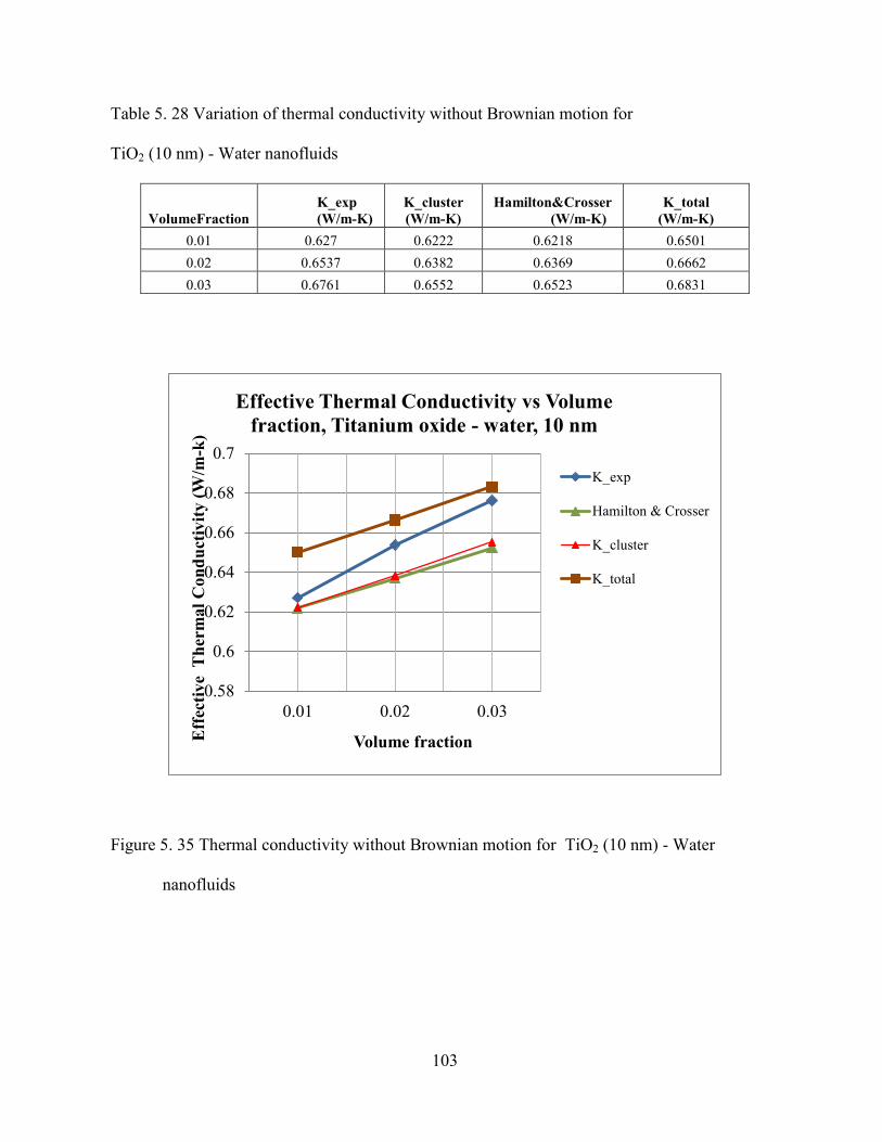
103



VolumeFraction

K_exp

(W/m-K)

K_cluster

(W/m-K)

Hamilton&Crosser

(W/m-K)

K_total

(W/m-K)

0.01 0.627 0.6222 0.6218 0.6501

0.02 0.6537 0.6382 0.6369 0.6662

0.03 0.6761 0.6552 0.6523 0.6831


nanofluids

0.58

0.6

0.62

0.64

0.66

0.68

0.7

0.01 0.02 0.03

Eff

ecti

ve

Th

erm

al

Con

du

ctiv

ity (

W/m

-k)

Volume fraction


fraction, Titanium oxide - water, 10 nm

K_exp

Hamilton & Crosser

K_cluster

K_total

104

Table 5. 29 Variation of thermal conductivity without Brownian motion for TiO2 (34 nm) -

Water nanofluids

VolumeFraction

K_exp

(W/m-K)

K_cluster

(W/m-K)

Hamilton&Crosser

(W/m-K)

K_total

(W/m-K)

0.01 0.6239 0.6221 0.6218 0.6307

0.02 0.6452 0.6380 0.6369 0.6465

0.03 0.6598 0.6547 0.6523 0.6632


nanofluids

0.6

0.61

0.62

0.63

0.64

0.65

0.66

0.67

0.01 0.02 0.03

Eff

ecti

ve

Th

erm

al

Con

du

ctiv

ity

(W/m

-K)

Volume Fraction



K_exp

Hamilton &

Crosser

K_cluster

K_total

105

Table 5. 30 Variation of thermal conductivity without Brownian motion for TiO2 (34 nm) – EG

nanofluids

VolumeFraction

K_exp

(W/m-K)

K_cluster

(W/m-K)

Hamilton&Crosser

(W/m-K)

K_total

(W/m-K)

0.01 0.261 0.2591 0.2589 0.2648

0.02 0.2719 0.2666 0.267 0.2723

0.03 0.2829 0.2745 0.2733 0.2802

Figure 5. 37 Thermal conductivity without Brownian motion for TiO2 (34 nm) –

EG nanofluids

0.24

0.245

0.25

0.255

0.26

0.265

0.27

0.275

0.28

0.285

0.29

0.01 0.02 0.03

Eff

ecti

ve

ther

mal

con

du

ctiv

ity (

W/m

-

K)

Volume fraction

Effective thermal conductivity vs volume fraction,

Titanium oxide, EG 34 nm

K_exp

Hamilton &

Crosser

K_cluster

K_total

106

Table 5. 31 Variation of thermal conductivity without Brownian motion for ZnO (10 nm) -

Water nanofluids

VolumeFraction K_exp (W/m-K)

K_cluster

(W/m-K)

Hamilton&Crosser

(W/m-K)

K_total

(W/m-K)

0.01 0.6367 0.6246 0.6242 0.6526

0.02 0.6652 0.6433 0.6419 0.6713

0.03 0.6931 0.6631 0.6579 0.6911

Figure 5. 38 Thermal conductivity without Brownian motion for ZnO (10 nm) –

Water nanofluids

0.58

0.6

0.62

0.64

0.66

0.68

0.7

0.01 0.02 0.03

Eff

ecti

ve

Th

erm

al

Con

du

ctiv

ity

(W/m

-K)

Volume Fraction


Fraction for ZnO-water, 10 nm

K_exp

Hamilton

&Crosser

K_cluster

K_total

107

Table 5. 32 Variation of thermal conductivity without Brownian motion for ZnO (30 nm) -

Water nanofluids

Volume

Fraction

K_exp

(W/m-K)

K_cluster

(W/m-K)

Hamilton&

Crosser (W/m-K)

K_total

(W/m-K)

0.01 0.627 0.6246 0.6242 0.6342

0.02 0.65 0.6431 0.6419 0.6527

0.03 0.6768 0.6626 0.6598 0.6722

Figure 5. 39 Thermal conductivity without Brownian motion for ZnO (30 nm) - Water

nanofluids

0.58

0.6

0.62

0.64

0.66

0.68

0.7

0.72

0.74

0.01 0.02 0.03

Eff

ecti

ve

ther

nal

con

du

ctiv

ity (

W/m

-K)

Volume fraction


ZnO- Water 30 nm

K_exp

Hamilton &

Crosser

K_cluster

K_total

108

Table 5. 33 Variation of thermal conductivity without Brownian motion for ZnO (60 nm) – EG

nanofluids

Volume

Fraction

K_exp

(W/m-K)

K_cluster

(W/m-K)

Hamilton&Crosser

(W/m-K)

K_total

(W/m-K)

0.01 0.2601 0.2596 0.2594 0.2628

0.02 0.2699 0.2675 0.267 0.2708

0.03 0.279 0.2759 0.2747 0.2792

Figure 5. 40 Thermal conductivity without Brownian motion for ZnO (60 nm) – EG nanofluids

0.245

0.25

0.255

0.26

0.265

0.27

0.275

0.28

0.285

0.01 0.02 0.03

Eff

ecti

ve

ther

nal

con

du

ctiv

ity (

W/m

-K)

Volume fraction


fraction, ZnO-EG, 60 nm

K_exp

Hamilton &

Crosser

K_cluster

K_total

109

Table 5. 34 Variation of thermal conductivity without Brownian motion for Al (20 nm) - Water

nanofluids

Volume

Fraction

K_exp

(W/m-K)

K_cluster

(W/m-K)

Hamilton&Crosser

(W/m-K)

K_total

(W/m-K)

0.01 0.6344 0.6315 0.6314 0.6460

0.02 0.6589 0.6506 0.6502 0.6651

0.03 0.6877 0.6703 0.6694 0.6848

Figure 5. 41 Thermal conductivity without Brownian motion for Al (20 nm) - Water nanofluids

The mathematical models were solved without the Brownian motion and the graphs

were plotted aga nst exper menta data’s pu shed and am ton-Crosser equation for various

combinations of nanofluids and the total thermal conductivity values. The above graphs lie on

par with the Hamilton-Crosser equation values, which validates that the mathematical model.

The graphs also shows that the thermal conductivity values lie below the experimental values,

which indicate that the Brownian motion contributes to the thermal conductivity enhancements

0.6

0.65

0.7

0.75

0.8

0.85

0.01 0.02 0.03Eff

ecti

ve

ther

mn

al

con

du

ctiv

ity

(W/m

K)

Volume fractioin


Al - Water, 20 nm

K_exp

Hamilton & Crosser

K_cluster

K_total

110

in nanofluids. It was found that the contribution of Brownian Motion was around 5% in lower

nanoparticle size ( 10 nm) and gradually decreased as the nanoparticle size increases. This also

validates the mathematical data developed. The size increase of the nanoparticle may have less

Brownian Motion thereby having a low impact in larger nanoparticles.

D. Effect of Cluster Stacking

The final parametric study that was done to study the effect of thermal conductivity by

stacking the nanoclusters. The clusters were assumed to stack together and the effective lengths

of the clusters were assumed to range from 0.33 to 2. The mathematical model was solved for

volume fractions 0.01 to 0.04. The values were plot as shown below for various nanofluid

combinations.

Table 5. 35 Effect of Cluster Stacking CuO ( 18 nm) – Water nanofluids

Mean Volume Fraction

cunit cell 0.01 0.02 0.03 0.04

0.33 0.6840 0.7022 0.7215 0.7418

0.5 0.6657 0.6839 0.7032 0.7235

1 0.6480 0.6662 0.6854 0.7058

1.2599 0.6443 0.6625 0.6818 0.7021

1.4423 0.6426 0.6607 0.6800 0.7003

1.5874 0.6414 0.6596 0.6788 0.6992

1.71 0.6406 0.6588 0.6780 0.6984

1.8171 0.6400 0.6582 0.6774 0.6978

1.9129 0.6395 0.6577 0.6769 0.6973

2 0.6391 0.6573 0.6765 0.6969

111

Figure 5. 42 Effect of Cluster Stacking on thermal conductivity for CuO(18 nm) –Water

nanofluids

Table 5. 36 Effect of Cluster Stacking CuO (23.6 nm) – Water nanofluids

Number of Volume Fraction

cunit cell 0.01 0.02 0.03 0.04

0.33 0.6840 0.7022 0.7215 0.7418

0.5 0.6657 0.6839 0.7032 0.7235

1 0.6480 0.6662 0.6854 0.7058

1.2599 0.6443 0.6625 0.6818 0.7021

1.4423 0.6426 0.6607 0.6800 0.7003

1.5874 0.6414 0.6596 0.6788 0.6992

1.71 0.6406 0.6588 0.6780 0.6984

1.8171 0.6400 0.6582 0.6774 0.6978

1.9129 0.6395 0.6577 0.6769 0.6973

2 0.6391 0.6573 0.6765 0.6969

0.6200

0.6400

0.6600

0.6800

0.7000

0.7200

0.7400

0.7600

0 1 2 3

K_ef

f (W

/m-K

)

c/unit cell (-)

K_eff for CuO - Water 18 nm

0.01

0.02

0.03

0.04

112

Figure 5. 43 Effect of Cluster Stacking on thermal conductivity for CuO (23.6 nm)–

Water nanofluids

Table 5. 37 Effect of Cluster Stacking CuO (30.8 nm) – EG nanofluids


cunit cell 0.01 0.02 0.03 0.04

0.33 0.2786 0.2866 0.2950 0.3040

0.5 0.2721 0.2801 0.2886 0.2976

1 0.2658 0.2739 0.2823 0.2913

1.2599 0.2646 0.2726 0.2810 0.2900

1.4423 0.2639 0.2719 0.2804 0.2894

1.5874 0.2635 0.2715 0.2800 0.2890

1.71 0.2632 0.2713 0.2797 0.2887

1.8171 0.2630 0.2710 0.2795 0.2885

1.9129 0.2629 0.2709 0.2793 0.2883

2 0.2627 0.2707 0.2792 0.2882

0.6200

0.6400

0.6600

0.6800

0.7000

0.7200

0.7400

0 1 2 3

K_ef

f (W

/m-K

)

K_eff for CuO - Water 23.6 nm

0.01

0.02

0.03

0.04

113

Figure 5. 44 Effect of Cluster Stacking on thermal conductivity


Table 5. 38 Effect of Cluster Stacking Al2O3 (60.4 nm) – Water

nanofluids


cunit cell 0.01 0.02 0.03 0.04

0.33 0.6459 0.6649 0.6849 0.7061

0.5 0.6409 0.6599 0.6799 0.7010

1 0.6360 0.6550 0.6750 0.6961

1.2599 0.6350 0.6540 0.6740 0.6951

1.4423 0.6345 0.6535 0.6735 0.6946

1.5874 0.6341 0.6532 0.6732 0.6943

1.71 0.6339 0.6529 0.6730 0.6941

1.8171 0.6338 0.6528 0.6728 0.6939

1.9129 0.6336 0.6526 0.6727 0.6938

2 0.6335 0.6525 0.6725 0.6937

0.2600

0.2650

0.2700

0.2750

0.2800

0.2850

0.2900

0.2950

0.3000

0.3050

0.3100

0 0.5 1 1.5 2 2.5

K_ef

f (W

/m-K

)

K_eff for CuO - EG 30.8 nm

0.01

0.02

0.03

0.04

114

Figure 5. 45 Effect of Cluster Stacking on thermal conductivity Al2O3 (60.4 nm) – Water

nanofluids

Table 5. 39 Effect of Cluster Stacking Al2O3 (26 nm) – EG nanofluids


cunit cell 0.01 0.02 0.03 0.04

0.33 0.2820 0.2900 0.2986 0.3076

0.5 0.2744 0.2824 0.2910 0.3000

1 0.2670 0.2751 0.2836 0.2926

1.2599 0.2655 0.2735 0.2821 0.2911

1.4423 0.2647 0.2728 0.2813 0.2904

1.5874 0.2643 0.2723 0.2809 0.2899

1.71 0.2639 0.2720 0.2805 0.2896

1.8171 0.2637 0.2718 0.2803 0.2893

1.9129 0.2635 0.2716 0.2801 0.2891

2 0.2633 0.2714 0.2799 0.2890

0.6200

0.6300

0.6400

0.6500

0.6600

0.6700

0.6800

0.6900

0.7000

0.7100

0 0.5 1 1.5 2 2.5

K_ef

f (W

/m-K

)

K_eff for Al2O3-Water 60.4 nm

0.01

0.02

0.03

0.04

115

Figure 5. 46 Effect of Cluster Stacking on thermal conductivity for Al2O3 (26 nm) – EG

nanofluids

Table 5. 40 Effect of Cluster Stacking TiO2 (10 nm) – Water nanofluids


cunit cell 0.01 0.02 0.03 0.04

0.33 0.7070 0.7230 0.7400 0.7580

0.5 0.6781 0.6942 0.7111 0.7291

1 0.6501 0.6662 0.6831 0.7012

1.2599 0.6444 0.6604 0.6774 0.6954

1.4423 0.6416 0.6576 0.6746 0.6926

1.5874 0.6398 0.6558 0.6728 0.6908

1.71 0.6385 0.6546 0.6715 0.6895

1.8171 0.6376 0.6536 0.6706 0.6886

1.9129 0.6368 0.6528 0.6698 0.6878

2 0.6362 0.6522 0.6692 0.6872

0.2600

0.2650

0.2700

0.2750

0.2800

0.2850

0.2900

0.2950

0.3000

0.3050

0.3100

0 0.5 1 1.5 2 2.5

K_ef

f (W

/m-K

)

K_eff for Al2O3-EG 26 nm

0.01

0.02

0.03

0.04

116

Figure 5. 47 Effect of Cluster Stacking on thermal conductivity for

TiO2 (10 nm) – Water nanofluids



cunit cell 0.01 0.02 0.03 0.04

0.33 0.6480 0.6639 0.6806 0.6982

0.5 0.6392 0.6551 0.6718 0.6893

1 0.6307 0.6465 0.6632 0.6808

1.2599 0.6289 0.6448 0.6615 0.6790

1.4423 0.6280 0.6439 0.6606 0.6782

1.5874 0.6275 0.6434 0.6601 0.6776

1.71 0.6271 0.6430 0.6597 0.6772

1.8171 0.6268 0.6427 0.6594 0.6769

1.9129 0.6266 0.6425 0.6591 0.6767

2 0.6264 0.6423 0.6589 0.6765

0.6200

0.6400

0.6600

0.6800

0.7000

0.7200

0.7400

0.7600

0.7800

0 0.5 1 1.5 2 2.5

K_ef

f (W

/m-K

)

K_eff for TiO2-Water 10 nm

0.01

0.02

0.03

0.04

117


nanofluids



cunit cell 0.01 0.02 0.03 0.04

0.33 0.6611 0.6771 0.6939 0.7117

0.5 0.6499 0.6659 0.6828 0.7005

1 0.6391 0.6551 0.6719 0.6897

1.2599 0.6368 0.6528 0.6697 0.6874

1.4423 0.6357 0.6518 0.6686 0.6864

1.5874 0.6351 0.6511 0.6679 0.6857

1.71 0.6346 0.6506 0.6674 0.6852

1.8171 0.6342 0.6502 0.6671 0.6848

1.9129 0.6339 0.6499 0.6668 0.6845

2 0.6337 0.6497 0.6665 0.6843

0.6200

0.6300

0.6400

0.6500

0.6600

0.6700

0.6800

0.6900

0.7000

0.7100

0 0.5 1 1.5 2 2.5

K_ef

f (W

/m-K

)


0.01

0.02

0.03

0.04

118


nanofluids

Table 5. 43 Effect of Cluster Stacking TiO2 (34 nm) – EG nanofluids


cunit cell 0.01 0.02 0.03 0.04

0.33 0.2763 0.2838 0.2917 0.3000

0.5 0.2705 0.2779 0.2858 0.2942

1 0.2648 0.2723 0.2802 0.2885

1.2599 0.2636 0.2711 0.2790 0.2873

1.4423 0.2630 0.2705 0.2784 0.2868

1.5874 0.2627 0.2702 0.2780 0.2864

1.71 0.2624 0.2699 0.2778 0.2861

1.8171 0.2622 0.2697 0.2776 0.2859

1.9129 0.2621 0.2695 0.2774 0.2858

2 0.2619 0.2694 0.2773 0.2857

0.6200

0.6300

0.6400

0.6500

0.6600

0.6700

0.6800

0.6900

0.7000

0.7100

0.7200

0 0.5 1 1.5 2 2.5

K_ef

f (W

/m-K

)


0.01

0.02

0.03

0.04

119

Figure 5. 50 Effect of Cluster Stacking on thermal conductivity for TiO2 (34 nm) – EG

nanofluids

Table 5. 44 Effect of Cluster Stacking ZnO (10 nm) – Water nanofluids


cunit cell 0.01 0.02 0.03 0.04

0.33 0.7094 0.7281 0.7479 0.7690

0.5 0.6806 0.6993 0.7191 0.7402

1 0.6526 0.6713 0.6911 0.7122

1.2599 0.6468 0.6655 0.6853 0.7064

1.4423 0.6440 0.6627 0.6825 0.7036

1.5874 0.6422 0.6609 0.6807 0.7018

1.71 0.6410 0.6596 0.6795 0.7006

1.8171 0.6400 0.6587 0.6785 0.6996

1.9129 0.6392 0.6579 0.6777 0.6988

2 0.6386 0.6573 0.6771 0.6982

0.2600

0.2650

0.2700

0.2750

0.2800

0.2850

0.2900

0.2950

0.3000

0.3050

0 0.5 1 1.5 2 2.5

K_

eff

(W/m

-K)

K_eff for TiO2-EG 34 nm

0.01

0.02

0.03

0.04

120

Figure 5. 51 Effect of Cluster Stacking on thermal conductivity for ZnO (10 nm) – Water

nanofluids

The above graphs indicate that the thermal conductivity decreases as the nanoclusters

begin to stack. There is a steep reduction in thermal conductivity as the nanocluster is divided in

half and then decreases linearly when the clusters join to combine. Further study can be done to

find out the reason behind the strange behavior.

E. Discussion of results of the parametric studies

Based on the preliminary results and validation, it is found that the clustering of

nanoparticles in a nanofluid, the nanolayer thickness around the nanoparticles and the Brownian

motion play a critical role in the thermal conductivity enhancement of nanofluids. The

mathematical model developed lies on par with experimental data which confirms that the

assumptions made for the development of mathematical model are accurate and well within the

practical limitations. The contribution due to the Brownian motion due to moving nanoparticles

in nanofluids is negligible when compared to the clustering effect of nanoparticles. The effect of

0.6000

0.6500

0.7000

0.7500

0.8000

0.8500

0.9000

0 0.5 1 1.5 2 2.5

K_ef

f (W

/m-K

)

K_eff for ZnO-Water 10 nm

0.01

0.02

0.03

0.04

121

nanoparticle diameter on the Brownian motion will be further analyzed using different sample

sets from various research and experimental data. The influence of zeta potential and the

nanolayer thickness will also be further analyzed. The factors governing the overall

enhancement of thermal conductivity will be understood better by solving the mathematical

model using the various assumptions. Validation of these results will provide an insight to

increase the thermal conductivity of nanofluids.

122

CHAPTER 6

CONCLUSION

A model for effective thermal conductivity of nanofluids was developed based on the

clustering of nanoparticles, nanolayer thickness, Brownian motion of the nanoparticle and

volume fraction of nanoclusters. The mathematical model developed to calculate the thermal

conductivity is a function of the thermal conductivities of the fluid and the nanoparticle,

clustering effect, the nanolayer, volume fraction, nanoparticle diameter. The developed equation

was compared to other models in the literature to understand the proximity of the results.

Parametric studies were conducted to know the effect of different factors on thermal

conductivity of nanofluids.

Based on the results obtained and validation, it is found that the clustering of

nanoparticles in a nanofluid, the nanolayer thickness around the nanoparticles and the Brownian

motion play a critical role in the thermal conductivity enhancement of nanofluids. The

mathematical model developed lies on par with experimental data which confirms that the

assumptions made for the development of mathematical model are accurate and well within the

practical limitations. The contribution due to the Brownian motion due to moving nanoparticles

in nanofluids is negligible when compared to the clustering effect of nanoparticles. The factors

governing the overall enhancement of thermal conductivity is also understood better by solving

the mathematical model using the various assumptions.

The conclusions drawn from this study are as follows: Kinetic theory was found to be

negligible in explaining the thermal conductivity behavior of nanofluids. Clustering of the

particles proved to be an important factor in enhancing the thermal conductivity of the

123

nanofluids. The model developed was found to be applicable for almost all the nanofluids.

Thermal conductivity of nanofluids increases with increase in the concentration of the

nanoparticles, nanolayer thickness and spherical clustering of nanofluids. The thermal

conductivity of nanofluids decreases with increase in the diameter of the nanoparticles.

Overall, the model predictions were found to be in good agreement with experimental

data. The study can be further scrutinized by varying some of the parameters such as

nanocluster structure formation, such as a nanoparticle chain, the effect on thermal conductivity

when the nanoparticle combine to form various shapes based on the surface charge in the

nanoparticle and the base fluid. The mathematical model solved for nanolayer thickness resulted

in decreased thermal conductivity for low volume fraction 0.01 and remained almost steady for

volume fractions 0.02 and 0.03 and increased at 0.04 volume fraction. Exploring the limiting

factors based on this result can be a topic for future studies. So this advanced technology of

suspending nanoparticles in base fluids might provide answers to improved thermal

management. Improved understanding of complex nanofluids will have an even broader impact.

124

REFERENCES

1. ang, B. ., Sheng, .Y., and Peng, .F., , “A nove stat st ca c uster ng mode for

pred ct ng therma conduct v t of nanof u d”, Internat ona ourna of Thermoph s cs, 30, pp.

1992-1998.

. V s nee, T., and Somcha , ., 1 , ‘‘Cr t ca rev e of heat transfer characteristics of Nano

fluids, Renewable and Sustainable Energy Reviews, 11, pp. 512-523.

3. L u, .S., L n, .C.C., uang, I.T., and , C.C., 6, “Enhancement of therma

conductivity with CuO for Nanofluids, Chemical Engineering and Technology, 29,

pp. 72-77.

4. K a , K., and K m, C., 5, “V scos t and therma conduct v t of copper ox de nanof u d

d spersed n eth ene g co ”, Korea-Australia Rheology Journal, 17, pp. 35-40.

5. L , Q., and uan, Y. ., , “Convect ve heat transfer and flow characteristics of Cu–

ater nano f u d”, Science in China, 45E, pp. 408–416.

6. Guo, S. Z., L , Y., ang, . S., e, . Q., 1 , “Nanof u ds Conta n ng gamma- -

Fe2O3 Nanopart c es and The r eat Transfer Enhancements”, Nanosca e es Lett, pp. 1222-

1227.

7. ang, . Q., ujumdar, A. S., , “ eat transfer character st cs of nanof u ds: a rev e ”,

International Journal of Thermal Sciences, 46, pp. 1-19.

8. Pa e , K., effre , A., and av d, G. C., 5, “Nanof u ds for therma transport”, ater a s

today, 8, pp. 36-44.

125

. V ja , K. K., “ ode for energ transport n nanof u ds”

10. Eapen, ., L , ., and Y p, S., 6, “Pro ng transport mechan sms n nanofluids by

mo ecu ar d nam cs s mu at ons”, Proceed ng of the 18th Nat ona and th IS T–ASME

Heat and Mass Transfer Conference, IIT Guwahati, India.

11. Ke ns , P., Ph pot, S. ., Cho , S. U. S., and Eastman, . A., , “ echan sms of heat

flow in suspensions of nano-s zed part c es (nanof u ds)”, Internat ona ourna of eat and

Mass Transfer, 45, pp. 855-863.

12. Eapen, J., 2004, “ ode ng Transport echan sm n Nanof u ds”, Project Report. 2.57,

Nano–to–Micro Transport Processes.

13. uan, Y., L , Q., and u, ., , “Aggregated Structure and Therma Conduct v t of

Nanof u ds”, AIChE ourna , 49, pp.1038-1043.

14. Shu a, . K., and h r, V. K., 5, “Stud of the effect ve therma conduct v t of

nanof u ds”, AS E Internat ona echan ca Eng neer ng Congress and Expos t on, F or da,

USA.

15. Prasher, R., Phelan, P. E., and Bhattacharya, P., 2006, “Effect of Aggregat on net cs on

the Therma conduct v t of nanosca e co o da so ut ons”, NANO LETTE S, 6, pp. 1529-

1534.

16. Prasher, ., Bhattachar a, P., and Phe an, P. E., 5, “Therma Conduct v t of Nanosca e

Colloidal Solutions (Nanofluids)”, The Amer can Ph s ca Soc et , 94, pp.

025901-1- 025901-4.

17. Feng, Y., Yu, B., u P., and Zou ., , “The effect ve therma conduct v t of

nanof u ds ased on the nano a er and the aggregat on of nanopart c es”, ourna of Ph s cs :

Applied Physics, 40, pp. 3164-3171.

http://www.tandfonline.com/action/doSearch?action=runSearch&type=advanced&result=true&prevSearch=%2Bauthorsfield%3A(Eapen%2C+J.)

126

18. XU, J., Bo-Ming, Y., and Mei- uan, Y., 6, “Effect of C usters on Therma conduct v t

n Nanof u ds”, Ch nese ph s cs etters, 23, pp. 2819- 2822.

19. Pate , . E., Sundararajan, T., and as, S. K., 6, “A ce approach model for thermal

conduct v t of nanof u ds”, ourna of Nanopart c e esearch, 10, pp. 87-97.

20. Prasher, P., Evans, ., F sh, ., ea n, P., Phe an, P., and Ke ns , P., 6, “Effect of

Aggregat on on Therma Conduct on n Co o da Nanof u ds”, Applied Physics Letters, 89, pp.

143119-1-143119-3.

21. Patel, H. E., Sundararajan, T., Pradeep, T., Dasgupta, A., Dasgupta, N., and Das, S. K.,

5, “A m cro-convect on mode for therma conduct v t of nanof u ds”, ourna of Ph s cs,

65, pp. 863-869.

22. urugesan, C., S van, S., 1 , “L m ts for therma conduct v t of nanof u ds” Therma

Science, 14, pp 65-71.

23. Tr sa sr , V., ong ses, S., , “Cr t ca rev e of heat transfer character st cs of

nanof u ds”, ene a e and Susta na e Energ ev e s, 11, pp. 512-523.

24. Zhou, L. P., ang, B. ., Peng, . F., u, . Z., Yang, Y. P., , “ On the spec f c heat

capac t of CuO”, Advances n echan ca Eng neer ng, 2010, pp 1-4.

25. Evans, ., F sh, ., and Ke ns , P., 6, “ o e of Bro n an mot on hydrodynamics on

nanof u d therma conduct v t ”, Amer can Inst tute of Ph s cs, 88, pp. 093116-1 – 093116-3.

26. Sh ma, P., ., Ph p, ., aj, B., , “ o e of m cro convent on nduced ro n an

motion of nanoparticles in the enhanced thermal conduct v t of sta e nanof u ds”, App ed

Physics Letters, 94, 223101-1-223101-3.

27. Kath e an, N. ., Ph p, ., aj, B., 8, “Effect of c uster ng on the therma conduct v t

of nanof u ds”, ater a s Chem str and Ph s cs, 109, pp. 50-55.

127

28. Hong, K.S., Hong, T-.K., Yang, H-.S., 6, “Therma conduct v t of Fe nanof u ds

depend ng on the c uster s ze of nanopart c es” App ed Ph s cs Letters, 88, pp. 031901-1-

031901-3.

29. u, C., Cho, T. ., u, ., Lee, ., Yang, B., Zachar ah, . ., 1 , “Effect of nanopart c e

c uster ng on the effect ve therma conduct v t of concentrated s ca co o ds”, Ph s ca

Review E, 81, pp. 011406-1-011406-6.

30. Lee, ., K m, . ., K m, B.G., 6, “A ne parameter to contro heat transport n

nanof u ds: Surface charge state of the part c e n suspens on”, The ourna of Ph s ca

Chemistry B, 110, pp. 4323-4328.

31. Xuan, Y., Li, Q., Zhang, X., and Fujii, M., 20 6, “Stochast c therma transport of

nanopart c e suspens ons”, ourna of App ed Ph s cs, 100, pp. 043507-1 – 043507-6.

32. am ton, .L., and Crosser, O.K., 1 6 , “Therma Conduct v t of heterogeneous t o-

component systems, I&EC Fundamentals, 1, pp. 182-191.

33. Koo, ., and K e nstreuer, C., 5, “A ne therma conduct v t mode for nanof u ds”,

Journal of Nanoparticle Research, 6, pp. 577-588.

34. Kang, . U., K m, S. ., and Oh, . ., 6, “Est mat on of Therma Conduct v t of

Nanofluid Using Exper menta Effect ve Part c e Vo ume”, Exper menta eat Transfer, 19, pp.

181-191.

35. ang, S.P., and Cho , S.U.S., 4, “ o e of Bro n an mot on n the enhanced therma

conduct v t of nanof u ds”, App ed Ph s cs etter, 84, pp. 4316-4318.

36. Bejan, A., 4, “Convect on eat Transfer”, rd

edition, John Wiley & sons.

128

. Prasher, P., Bhattachar a, P., and Phe an, P. E., 6, “Bro n an-Motion-Based

Convective-Conduct ve ode for the Effect ve Therma Conduct v t of Nanof u ds”, ourna

of Heat Transfer, 128, pp. 588-595.

38. ang, S.P., and Cho , S.U.S., , “Effects of var ous parameters on Nanof u d Therma

Conduct v t ”, ourna of eat Transfer, 129, pp. 617- 623.

39. Kumar, H. D., Patel, H. E., Kumar, R. V. R., Sundararajan, T., Pradeep, T., and Das, S. K.,

4, “ ode for eat Conduct on n Nanof u ds”, The Amer can Ph s ca Soc et , 93, pp.

144301-1 – 144301-4.

40. Feng, Y., Yu, B., u, P., Zou, ., 8, “Therma conduct v t of nanof u ds and s ze

distribution of nanoparticles by Monte Car o s mu at ons”, ourna of Nanopart c e esearch.

41. B rd, B. ., Ste art, . E., and L ghtfoot, E. N., , “Transport Phenomenon”, Second

Edition, John Wiley & sons, Inc.

42. ang, B. ., Zhou, L. P., and Peng, . F., , “A fracta mode for predicting the

effect ve therma conduct v t of u d th suspens on of nanopart c es”, Internat ona ourna

of Heat and Mass transfer, 46, pp. 2265-2672.

43. Yu, B., Z, ., and F, Y., 5, “Permea t of fracta porous med a onte Car o

Simulations”, Internat ona ourna of eat and ass transfer, 48, pp. 2787-2794.

44. Timofeeva, E. V., Gavrilov, A. N., McCloskey, J. M., and Tolmachev, Y. V., 2007,

“Therma conduct v t and part c e aggregat on n a um na nanof u ds: Exper ment and theor ”,

The American Physical Society, 76, pp. 061203-1-061203-16.

45. Leong, K.C., Yang, C., and urshed, S. .S., 6, “A ne mode for therma conduct v t

of nanofluids – the effect of nterfac a a er”, ourna of Nanopart c e esearch, 8, pp. 245-254.

129

46. Jeffre , . ., 1 , “Conduct on through suspens on of spheres”, o a Soc et of London

Series A, Mathematical and Physical Sciences, 335, pp. 355-367.

47. Lee, S., Cho , S.U.S., L , S., and Eastman, . A., 1 , “ easur ng Therma Conduct v t

of fluids conta n ng ox de nanopart c es”, AS E . eat Transfer, 121, pp. 280-289.

48. Eastman, .A., Cho , S.U.S., L , S., Yu, ., and Thompson, L. ., 1, “Anoma ous

increased effective thermal conductivities of ethylene glycol-based nanofluids containing

copper nanopart c es”, Amer can Inst tute of Ph s cs, 78, pp. 718-720.

49. K m, S. ., Cho , S. ., and K m, ., , “Therma conduct v t of eta -Oxide

Nanof u ds: Part c e S ze ependence and Effect of Laser Irrad at on”, ourna of eat Transfer,

129, pp. 298-307.

50. ong, T.K., and Yang, .S., 5, “Stud of the enhanced therma conduct v t of Fe

nanof u ds”, ourna of App ed Ph s cs, 97, pp. 064311-1 – 064311-4.

51. T man, P., and , . ., 6, “A ne mode for Therma Conduct v t n Nanof u ds”,

IEEE , pp. 673-676.

52. Kang, . U. ., K m, S. ., and Oh, . ., 6, “Est mat on of Therma Conduct v t of

Nanof u d Us ng Exper menta Effect ve Part c e Vo ume”, Exper menta eat Transfer, 19, pp.

181-19.

130

APPENDICES

131

VITA

Graduate School

Southern Illinois University


[email protected]

Bharathiyar University

Bachelor of Engineering, Mechanical Engineering, May 2004

Thesis Title: Thermal Conductivity Enhancement of Nanofluids – Mathematical Model

Major Professor: Dr. Kanchan Mondal

mailto:[email protected]

thermal conductivity enhancement in nanofluids

Documents