Header for SPIE use

Theory of Geometrical Methods for Design of Laser Beam Shaping Systems

David L. Shealy∗

University of Alabama at Birmingham Department of Physics, 1530 3rd Avenue South, CH310

Birmingham, AL 35294-1170 USA

ABSTRACT From geometrical optics, the laws of reflection and refraction, ray tracing techniques, conservation of energy within a bundle of rays, and the condition of constant optical path length provide a foundation for design of laser beam shaping systems. Geometrical optics design methods are presented for shaping the irradiance profile of both rotationally and rectangular symmetric laser beams. Applications of these techniques to design reflective and refractive laser beam shaping systems are presented. Keywords: laser; beaming shaping; geometrical optics; optical design; irradiance mapping

1. INTRODUCTION Geometrical optics is used to shape the irradiance profile as part of the optical design of laser beam shaping systems. The laws of reflection and/or refraction, ray tracing, conservation of energy within a bundle of rays, and constant optical path length condition are used to design laser beam profile shaping optical systems. Interference or diffraction effects are not considered as part of the design process. Only lenses and mirrors are used for the optical components of the beam shaping systems presented in this paper. Reference 1 also describes how to use geometrical optics to design laser beam shaping systems.

There are many diverse applications of lasers in science and technology.2 These applications use a variety of the unique properties of lasers, such as, the high intensity, coherent, monochromatic light of lasers. For illumination applications, it is important for the laser beam to uniformly illuminate the target surface. Truncating a Gaussian beam with an aperture is a way to more uniformly illuminate the target surface with a laser beam. However, intensity apodization techniques are inefficient. Both reflective3, 4, 5 and refractive6, 7, 8 optical systems have been used to shape laser beam profiles.

McDermit and Horton3 use conservation of energy within a bundle of rays to design rotationally symmetric reflective optical systems for illuminating a receiver surface in a prescribed manner using a non-uniform input beam profile. Malyak5 has designed a two-mirror laser profile shaping system where the second mirror is decentered relative to the first mirror to eliminate the central obscuration present in the axially symmetric design for reflective systems. Cornwell9, 10 presents general results that can be used to design laser beam shaping systems with rotational, rectangular, or polar symmetry about the optical axis.

Kreuzer6 has patented a coherent-light optical system using two aspherical surfaces to yield an output beam of desired intensity distribution and wavefront shape. Rhodes and Shealy7 derived a set of differential equations using intensity mapping to calculate the shape of two-aspherical surfaces of a lens system that expands and converts a Gaussian laser beam profile into a collimated, uniform irradiance output beam. Using their method, two-plano-aspherical lenses have been designed, fabricated and used for laser beam shaping in a holographic projection system.11, 12, 13

A theory for designing the optics of a laser beam shaping system is presented in section 2. A brief overview of the concepts of rays, wavefronts, and energy propagation within geometrical optics is presented. Then, specific attention is devoted to using conservation of energy within a bundle of rays, ray tracing, and the constant optical path length condition as constraints on the optics figure of laser beam shaping systems. Section 3 presents three applications of this theory of laser beam shaping using one-mirror, two-lens, and two-mirror configurations.

Copyright 2000 Society of Photo-Optical Instrumentation Engineers. This paper will be published in Proc. SPIE 4095 and is made available as an electronic preprint with permission of SPIE. One print or electronic copy may be made for personal use only. Systematic or multiple reproduction, distribution of multiple locations via electronic or other means, duplication of any material in this paper for a fee or for commercial purposes, or modification of the content of the paper are prohibited.

∗ Other author information: E-mail: dls@uab.edu ; Telephone: 205-934-8068; Fax: 205-934-8042.

2. THEORY OF LASER BEAM SHAPING

2.1. Overview of the Concepts of Rays, Wavefronts, and Energy Propagation within Geometrical Optics The concepts of rays, wavefront, and energy propagation are fundamental to understanding and using geometrical optics14, 15

to design a laser beam shaping system. In order to determine or optimize the irradiance within an optical system, the optical field must be determined throughout the system. The optical field is a local plane wave solution of Maxwell's equations or the scalar wave equation.16, 17 For an isotropic, non-conducting, charge-free medium, the optical field may be written as:

u u ik S( ) ( ) exp ( )r r= 0 0 r (1)

where represents the components of the electric field at any point r , is the index of refraction at r , u( )r nk c0 = = 02ω π λ is the wave number in free space, ω is the frequency of the wave, c is the speed of light, and λ 0 is the wavelength of light. and are unknown functions of r . Requiring from Eq. (1) satisfy the scalar wave equation leads to the following conditions which must be satisfied by u and

u0( )r S( )r (r)u0(r) S( )r :

∇ =S nb g2 2 (2)

2 00 0 02 2u S u u S∇ ⋅∇ + ∇ = (3)

where the term proportional to 1 02kc h has been neglected. Equation (2) is known as the eikonal equation and is a basic

equation of geometrical optics. The surfaces S .x y z const( , , ) = are constant phase fronts of the optical field, have a constant optical path length from the source or reference surface, and are known as the geometrical wavefronts. For isotropic media, rays are normal to the wavefront. A unit vector normal to the wavefront and along a ray at the point r is given by

( )LOP

a r rr

rr

( ) ( )( )

( )( )

=∇∇

=∇S

SS

n. (4)

Equation (3) is equivalent to conservation of radiant energy within a bundle of rays and leads to the geometrical optics intensity law for propagation of a bundle of rays. Using the vector identity ∇⋅ = ∇⋅ + ⋅∇( )f fv v v f , Eq. (3) can be

rewritten as . Then, recognizing that the energy density of a field is proportional to the square

of the field amplitude u and that the intensity

∇⋅ ∇ = ∇⋅ =u S u n02

02 0c h c ha

o2 I is equal to the energy density of the field times the speed of propagation

within medium, Eq. (3) can be written as

( ) 0I∇⋅ =a . (5)

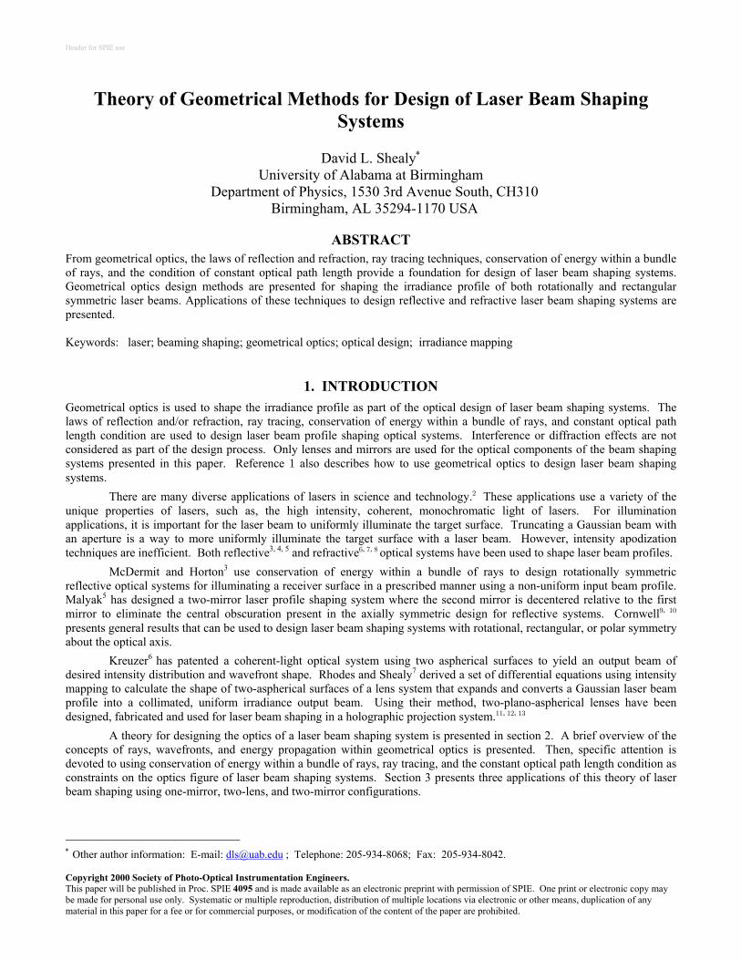
For beam shaping systems with collimated input and output beams as illustrated in Figure 1, a useful expression for the energy within a bundle of rays18 as it passes through the system follows by integrating Eq. (5) over reference planes (or wavefronts) normal to the input and output beam and then applying Gauss’ theorem

in outI dw I dW= . (6)

Equation (6) expresses conservation of energy along a bundle of rays between input element of area and the

corresponding output element of area dW on the wavefront or the reference planes normal to beam. Equation (6) is a basic equation used to design laser beam shaping systems.

( )2dw rdrπ=

( 2 Rdrπ= )

For some beam shaping configurations, it is necessary to introduce the conservation of energy condition into the optical design by using reference surfaces, such as for detectors, which are curved and/or have an arbitrary orientation with respect to the direction of the beam propagation. In these cases it is necessary to take into account projecting the element of

area of a reference surface perpendicular to direction of beam propagation when applying Eq. (6). Several examples will be presented later in this paper to illustrate cases using Eq. (6) as part of the design of laser beam shaping systems.

According to geometrical optics, the phase and amplitude of the optical field are evaluated independently. First, the ray paths are evaluated throughout the optical system, which enables computing the phase in terms of the optical path length of rays passing thought the system. The amplitude of the optical field is determined by monitoring the intensity variations along each ray.19, 20, 21

Figure 1. Schematic layout of a laser beam profile shaping system.

Rays generally characterize the direction of propagation of radiant energy, except near foci or the edge of a shadow where interference and diffraction takes place. As such, a ray is a mathematical construct rather than a physical quantity. Snell's law relates the direction of incident and refracted rays at an interface between media of different indices of refraction, which can be written in vector form22

′ = + ′ ′ −n n n i n iA a cos cos n (7)

where and are unit vectors along the incident and refracted rays, is a unit vector along the normal to the interface surface with the general orientation of the incident ray, ( ,

a A n)n n′ are the indices of refraction of the incident and refracting

media, are the angles of incidence and refraction, (i i, ′) ˆ and cos = ˆicos ,i′ = ⋅A n a n⋅ . When mirrors are involved, Eq. (7) can be used to compute the direction of the reflected ray by setting ′ = −n n and using the optics sign convention.23 Explicitly, a unit vector A along a reflected ray is given by

ˆ ˆ2 )= − ⋅A a n(a n . (8)

Beam propagation is commonly described by wavefronts. A wavefront is a surface of constant phase of the wave or optical path length from the source or reference surface. Each ray generally follows the path of shortest time through the optical system according to Fermat's Principle which states that a ray from points P to Q is the curve C connecting these two points such that the integral

(OPL)

dsOPL( ) ( , , )C

C n x y z= ∫ (9)

is an extremum (maximum, minimum, or stationary). The quantity is the index of refraction of the medium, and is the infinitesimal arc-length of the curve. For a homogeneous medium, the optical path length between P and Q is the

geometrical path length between the two points times the index of refraction of the medium. In general, the optical path length divided by the speed of light in free space, c , gives the time for light to travel from point P to Q along the ray path C. The ray path C can be determined using the calculus of variations.

n x y z( , , )ds

24 When the index of refraction, , is a smooth function, it can be shown

n( )r17 that the ray path C satisfies the differential equation

dds

n dds

n( ) ( )r r rFHG

IKJ = ∇ (10)

where is the position vector of any point on the ray. Equation (10) is known as the ray equation and is difficult to solve in many cases. For homogeneous medium ( ), the ray path is represented by a straight line

rn const=

r a( )s s= + b (11)

where and are constant vectors, and is the ray path length. Constant index of refraction materials are used in many optical systems. When the index of refraction is a function of position, such as, the axial distance, , the ray paths are curved.

a b sz

2.2. Conservation of Energy Condition An overview of using the conservation of energy condition to design laser beam shaping systems is presented in this section. First, systems in the configuration of Figure 1 are considered. It is shown how to relate the input and output beam diameters to conserve energy for a Gaussian input beam. Then, it is shown how to use conservation of energy, Eq. (6), to design beam shaping optics when a non-collimated output beam is incident upon a curved detector.

2.2.1. Collimated Input and Output Beams Assume the incident beam is a laser in the fundamental, Gaussian TEM00 mode with central intensity normalized to unity. Then,

20( ) exp[ 2( ) ]inI r r= − r (12)

where is the radius of the beam. The conventional definitionr025 of the diameter of a laser beam or waist is the location at

which the field amplitude is of its peak value. At the beam waist the beam intensity is of its axial value. For a Gaussian beam, 86.5% of the total energy of the beam is contained within the waist. This beam leaves the optical system at a radial distance

1e− 2e−

R from the optical axis with a power density of ( )outI R which is commonly sought to be constant as a result of the beam shaping design process.

Integrating Eq. (6) over the input and output planes gives

2 2

0 0 0 0

( ) ( )r R

in outd I r r dr d I R R dRπ π

θ θ=∫ ∫ ∫ ∫ (13)

where reflection and absorption losses have not been considered. When ( )outI R( )

is constant, the radius of beam in the exit aperture

R can be evaluated by carrying out the integration using Eq. (12) for inI r to obtain

( )2

2 2001 exp 2

2 out

rR r rI

= − − (14)

where

( )2

2 20out max 02

max

I 1 exp 22

r r rR

= − − . (15)

In Eq. (15), r is the working input aperture of the optical system, and is the corresponding point on the output plane. Equation (14) is used during the optical design process to reduce the number of independent variables and determine the shape of the reflecting or refracting surfaces of the beam shaping system. Equation (14) relates the output beam radius to that of input beam,

max Rmax

( )R r , for system configurations illustrated in Figure 1.

2.2.2. Uniform Irradiance over Curved Detector When a beam shaping system does not have either a collimated input or output beam as illustrated in Figure 1 or the output reference surface is curved, the conservation of energy condition, Eq. (6), needs to be revised to incorporate the actual geometry. In these cases, it is generally not possible to integrate the resulting conservation of energy condition [revised Eq. (6)] and then to solve for ( )R r as done in Eq. (14). Rather, the optical design of these types of beam shaping systems can

be accomplished by incorporating the mapping ( , of the ray trace equations into the expression of conservation of energy for the beam shaping system, and then solve the resulting differential equation for the contour of the reflecting or refracting surfaces. This procedure is illustrated in section 3.1 for a one-mirror beam shaping system.

) ,r z R Z⇒ b g

2.3. Ray Trace Equations For the refractive beam shaping system shown in Figure 2, rays are refracted at surface s according to Snell's law. The direction of refracted ray traveling from the point ( , on surface s to the point ( , on surface S is given by Eq. (7)

where the incident rays are along the optical axis, that is, aA )r z )R Z

k= . Explicitly, a unit vector along the refracted rays over surface s is given by

A k= +γ Ωn (16)

where 0n nγ = ; ( )z dz r d′ = r ; and

Ω =− + + ′ −

+ ′

γ γ1 1

1

2 21 2

2 1 2

z

z

b g c ho tb g

, (17)

n r k= − ′ + + ′z zd i b g1 2 1 2. (18)

The unit vectors are along the ( , )r k r z− directions. According to Eq. (11), the ray path connecting and ( , is a straight line with slope given by Eq. (16) and can be represented by

( , )r z )R Z

( )( ) ( )(R r Z zz r− = −A A) (19)

where and ( are the (r, z) components of given by Eq. (16). Combining Eqs. (16) and (19) yields, after squaring, collecting terms in powers of , and simplifying:

( )A r )A z A′z

1 22 2 2 2 2 2− − − − ′ + − − ′ + − =γ γc hb g b g b g b gb g b gZ z R r z R r Z z z R r 0 . (20)

In Eq. (20), R is given by Eq. (14), and is the solution to the differential equation as a function of the entrance aperture coordinate

zr . Z in Eq. (20) is not yet known. For beam shaping applications, which seek to illuminate a specific surface S

with uniform intensity, the equation of the surface S expressed as Z Z R= ( ) will be adequate to solve the differential equation (20) for the shape of the surface s. For other beam shaping applications, which seek to also control the shape of the output wavefront, the constant optical path length condition for rays passing through the system is used to determine the shapes of the surfaces s and S, when solved simultaneously with Eq. (20).

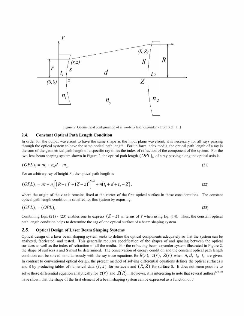
Figure 2. Geometrical configuration of a two-lens laser expander. (From Ref. 11.)

2.4. Constant Optical Path Length Condition In order for the output wavefront to have the same shape as the input plane wavefront, it is necessary for all rays passing through the optical system to have the same optical path length. For uniform index media, the optical path length of a ray is the sum of the geometrical path length of a specific ray times the index of refraction of the component of the system. For the two-lens beam shaping system shown in Figure 2, the optical path length ( of a ray passing along the optical axis is )

2

OPL 0

( )OPL nt n d nt0 1 0= + + . (21)

For an arbitrary ray of height r , the optical path length is

( )OPL nz n R r Z z n t d t Zr = + − + − + + + −02 2 1 2

1 2b g b g b g . (22)

where the origin of the z-axis remains fixed at the vertex of the first optical surface in these considerations. The constant optical path length condition is satisfied for this system by requiring

( ) ( )OPL OPL r0 = . (23)

Combining Eqs. (21) - (23) enables one to express ( )Z z− in terms of r when using Eq. (14). Thus, the constant optical path length condition helps to determine the sag of one optical surface of a beam shaping system.

2.5. Optical Design of Laser Beam Shaping Systems Optical design of a laser beam shaping system seeks to define the optical components adequately so that the system can be analyzed, fabricated, and tested. This generally requires specification of the shapes of and spacing between the optical surfaces as well as the index of refraction of all the media. For the refracting beam expander system illustrated in Figure 2, the shape of surfaces s and S must be determined. The conservation of energy condition and the constant optical path length condition can be solved simultaneously with the ray trace equations for when are given. In contrast to conventional optical design, the present method of solving differential equations defines the optical surfaces s and S by producing tables of numerical data for surface s and ( , for surface S. It does not seem possible to

solve these differential equation analytically for and . However, it is interesting to note that several authors

R r z r Z r( ), ( ), ( )

)R Z

n d t t, , ,1 2

( , )r zz r( ) Z Rb g 5, 9, 10

have shown that the shape of the first element of a beam shaping system can be expressed as a function of r

z r f r dr C( ) ( )= +z (24)

where C is a constant, and is a function relating to the optical configuration. The shape of the second surface can be computed from the following expression

f r( )

Z r z r g r( ) ( ) ( )= + (25)

where is another function from the configuration. Section 3 describes how to design a one-mirror, two-lens, and two-mirror beam shaping systems that can uniformly illuminate a detector with an input laser beam and expand or magnify the beam diameter.

g r( )

3. Optical Design of Laser Beam Shaping Systems The optical design of laser beam shaping systems involves incorporating the geometrical optics intensity law for propagation a bundle of rays (conservation of energy) and the constant optical path length condition into the ray trace equations for the optical system and then determining the geometrical shapes of several optical surfaces (or GRIN materials) so that the beam shaping design conditions are satisfied. For beam shaping applications that only need to illuminate a given surface with a specific irradiance distribution, the constant optical path length condition will not be part of the design process.

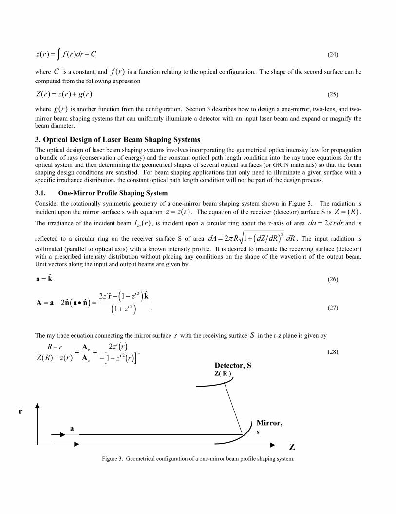
3.1. One-Mirror Profile Shaping System Consider the rotationally symmetric geometry of a one-mirror beam shaping system shown in Figure 3. The radiation is incident upon the mirror surface s with equation ( )z z r= . The equation of the receiver (detector) surface S is ( )Z R= .

The irradiance of the incident beam, ( )inI r , is incident upon a circular ring about the z-axis of area da 2 rdrπ= and is

reflected to a circular ring on the receiver surface S of area ( )22 1dA R dZ dR dRπ= + . The input radiation is collimated (parallel to optical axis) with a known intensity profile. It is desired to irradiate the receiving surface (detector) with a prescribed intensity distribution without placing any conditions on the shape of the wavefront of the output beam. Unit vectors along the input and output beams are given by

ˆ=a k (26)

( ) ( )( )

2

2

ˆˆ2 1ˆ ˆ2

1z z

z

′ ′− −= − • =

′+

r kA a n a n

. (27)

The ray trace equation connecting the mirror surface with the receiving surface s S in the r-z plane is given by

R rZ R z r

z rz r

r

z

−−

= =′

− − ′( ) ( )AA

21 2

b gb g . (28)

Detector, S Z( R )

r

Figure 3. Geometrical configuration of a one-mirror beam profil

a

Mirror,

s

e shaping system.

Z

Equation (28) can be written as

− − ′ + − ′ + − =R r z Z z z R rb g b g b g2 2 0 . (29)

Applying the differential energy balance Eq. (6) to this problem gives

( )2

1 22 22 ( )2 ( )2 1in out outdZI r rdr I R R dR dZ I R R dRdR

π π π = + = + . (30)

Displaying the term ( in Eq. (30) gives )dR dr

( )( ) 2

1

1

in

out

I rdR rdr I R R dZ

dR

= +

. (31)

Recall that ( ) ( )( ), , andin outI r I R Z R are known functions of their respective variables, and is an unknown function at this point of the analysis. Also, note that the ray trace Eq. (28) expresses a mapping between surfaces s and S:

z rb g

( , ) ,r z R Z⇒ b g (32)

which implies that R is a function of r, . By implicit differentiation of Eq. (29) with respect to r, it will be shown below how to incorporate the differential energy balance equation (31) into the ray trace equation for this problem, and therefore, obtain a differential equation for the unknown shape of the mirror surface s.

R rb g

Differentiating Eq. (29) with respect to r gives

− ′ ′′ − − ′ −FHGIKJ + ′′ − + ′ − ′L

NMOQP + −FHG

IKJ =2 1 2 22z z R r z dR

drz Z z z dZ

drz dR

drb g b g 1 0 . (33)

From the chain rule for differentiation of a function of a function, the term dZ drb in Eq. (33) can be written as gdZdr

dZdR

dRdr

Z R dRdr

= = ′( ) (34)

where ′ ≡Z R dZ R dR( ) b g can be evaluated directly from the equation of the surface S. Combining Eqs. (34) and (33) leads to

( ) ( ) ( )2 22 1 2dRz z R r Z z z z Z zdr

′′ ′ ′ ′ ′ ′ − − + − + − + − + = 1 0 . (35)

Rewriting Eq. (29) in the form

Z zR r

zz− =

−′

′ −b g b g2

12 , (36)

enables Eq. (35) to be written as

( ) ( ) ( )2 21 1 2 1z dRR r z z z Z zz dr′′ ′ ′ ′ ′ − − + + − + − + = ′

2 0′ . (37)

The term dR dr can be eliminated between Eqs. (31) and (37) , and then the following differential equation is used to

determine the sag : ( )z r

( )

( )( )

( )2

2 2

2

1 21 11 1

1

in

out

z z dZz dRzI rz r

z R r I R R dZdR

′ ′ − + ′ ′+ + ′′ = − ′ − +

. (38)

Equation (38) is equivalent to Eq. 13 of Ref. 3 and Eq. 3.14 of Ref. 4. When appropriate boundary conditions are given, Eq. (38) can be solved for the shape of the mirror used to illuminate the receiver surface S with a prescribed intensity ( )outI R

for a given source intensity profile ( )inI r . References 3 and 4 develop an extension of this analysis to two-mirror intensity profile shaping systems. A number of specific solutions for both one- and two-mirror systems are given in Refs. 3 and 4 including two laser beam profile shaping systems, such as, uniform illumination of a plane perpendicular to the incident beam using a one-mirror system for an input Gaussian beam, Fig. 7.3 of Ref. 4, and uniform illumination of a plane on the optical axis with a two-mirror system for an input Gaussian beam, Fig. 7.9 of Ref. 4.

3.2. Two-Lens Beam Shaping System For optical systems when the sag of two surfaces can be used in the optical design process, it is possible to shape the output beam intensity profile and to keep the optical path length constant (retain the wavefront shape) for all rays passing through the system. Further, it is often desirable to expand the laser beam diameter. To achieve these design goals, the optical surface shapes or index of refraction profiles may be used as design variables. Consider the geometrical configuration of a refracting laser beam profile shaping system shown in Figure 2. For applications using monochromatic laser beams, there are no chromatic aberrations present, and it is satisfactory to use the same material (index of refraction) for all lenses. The two curved surfaces (reflecting or refracting, depending on the application) are used to satisfy the design conditions for the beam shaping system.

Rays are refracted at surface s according to Snell's law. The direction of refracted ray traveling from the point on surface s to the point ( , on surface S is given by Eq. (16). The ray path connecting ( , and ( , is a

straight line according to Eq. (11) and is explicitly given by Eq. (19) which can be rearranged as a quadratic equation for

A( , )r z )R Z )r z )R Z

z′ , Eq. (20). Solving Eq. (20) as a quadratic equation for ′z gives

( ) ( ) ( ) ( ) ( ) ( )( ) ( ) ( ) ( )

2 20

2 2 2 20 0(1 )

R r Z z n n R r Z z R rz

n n Z z n n R r

− − − ± − − + −′ =

− − − − (39)

where the positive solution for is used for the laser shaping lens configuration shown in Figure 2 so that the first lens is divergent. For this lens system, the constant irradiance of the output beam is computed from Eq. (15); t e height of a ray

′zh R

at the second lens for each ray in the entrance pupil with height r is computed from Eq. (14). b is determine by the constant optical path length condition, Eqs. (21) - (23), or explicitly

Z z− g

n R r Z z n Z z d n n02 2 1 2

0− + − = − − −b g b g b g b g , (40)

which can be viewed as a quadratic equation for ( )Z z− as a function of entrance pupil aperture radius r . After squaring Eq. (40) and collecting terms, the solution of the resulting quadratic equation for ( )Z z− is

( )( ) ( ) ( )( )

Z zn n n d n n d n n R r

n n− =

− + − + − −

−0 0

2 2 2 202 2 1 2

202

1 (41)

where the positive sign of the radical has been used so that the solution reduces to the appropriate value of ( )Z z d− = when r R= = 0 .

It is interesting to note that combining Eqs. (39) and (41) permits ′z to be expressed as a function of r , thus, enabling to be evaluated by an integration, as illustrated in Eq. (24). Then, the shape of S is computed from Eq. (41), which has the functional form of Eq. (25). Cornwell

z r( )9, 10 and Malyak5 have reached a similar conclusion. Explicitly for the

two-lens beam shaping system shown in Figure 2, it follows from Eqs. (14) and (41)

( )

1 222 2

2 2 2 2 2 00 0 0 2

0

2 20

( ) ( 1) ( ) 1 exp 22

( )ou

r rn n n d n n d n n rI r

g r zn n

− + − + − − − − =−

t

Z= − . (42)

Similarly, comparing Eqs. (24) and (39) leads to the following expression for ( )f r

f r b r b r a r c ra r

( ) ( ) ( ) ( ) ( )( )

=− ± −2 24

2 (43)

where

( )( ) ( ) ( ) (2 22 20 0( ) 1a r n n g r n n c r= − − ) , (44)

b r c r g r( ) ( ) ( )= 2 , (45)

2 20

20

( ) ( ) 1 exp 22 out

r rc r R r rI r

= − = − − −

. (46)

Then, is determined by numerically integrating z ′z from Eq. (24) or (39), and Z is evaluated from Eq. (25) or (41). A FORTRAN program for computing ( , and is given in Appendix A of Ref. 12. Solving the differential equations using these programs defines the optical surfaces s and S by producing tables of numerical data ( , for surface s and

for surface S.

)r z ( , )R Z)r z

( ,R Z)To analyze the performance of these laser beam shaping optical systems with conventional optical design packages

(CODE V26, OSLO27, or ZEMAX28), the data representing the surfaces s and S has been fit to the conventional optics surface equation29 of a conic term plus rotationally symmetric aspherical deformation terms for the laser shaping system. The optics surface equation can be written in the

z rr

A rii

i

N

=+ − +

+=∑c

c2

2 2 22

11 1 1 κb g (47)

where (vertex curvature), c κ (conic constant), and (coefficients of the polynomial deformation terms) are surface parameters that are determined by the fitting process for each surface. A nonlinear least squares fitting program based on the simplex method

A i2

30 has been successfully used11, 12, 13 to represent the optical surfaces of a laser profile shaping system. The flux flow equation20 has been used to compute the irradiance along a ray as it propagates through the optical system.7, 8 Alternatively, radiometric calculations for optical systems can be performed by using “unit sphere” method19 or by writing a macro for optical design software package to compute the irradiance over an output surface of the laser shaping system.31 Reference 32 presents results for design, fabrication, and testing of a two-lens laser beam shaping system in the configuration shown in Figure 2.

3.3. Two-Mirror Beam Shaping System As the final application of the beam shaping theory developed in section 2, a two-mirror laser beam shaping system with rectangular symmetry will be described. For more details and applications of two-mirror beam shaping optics, the interested

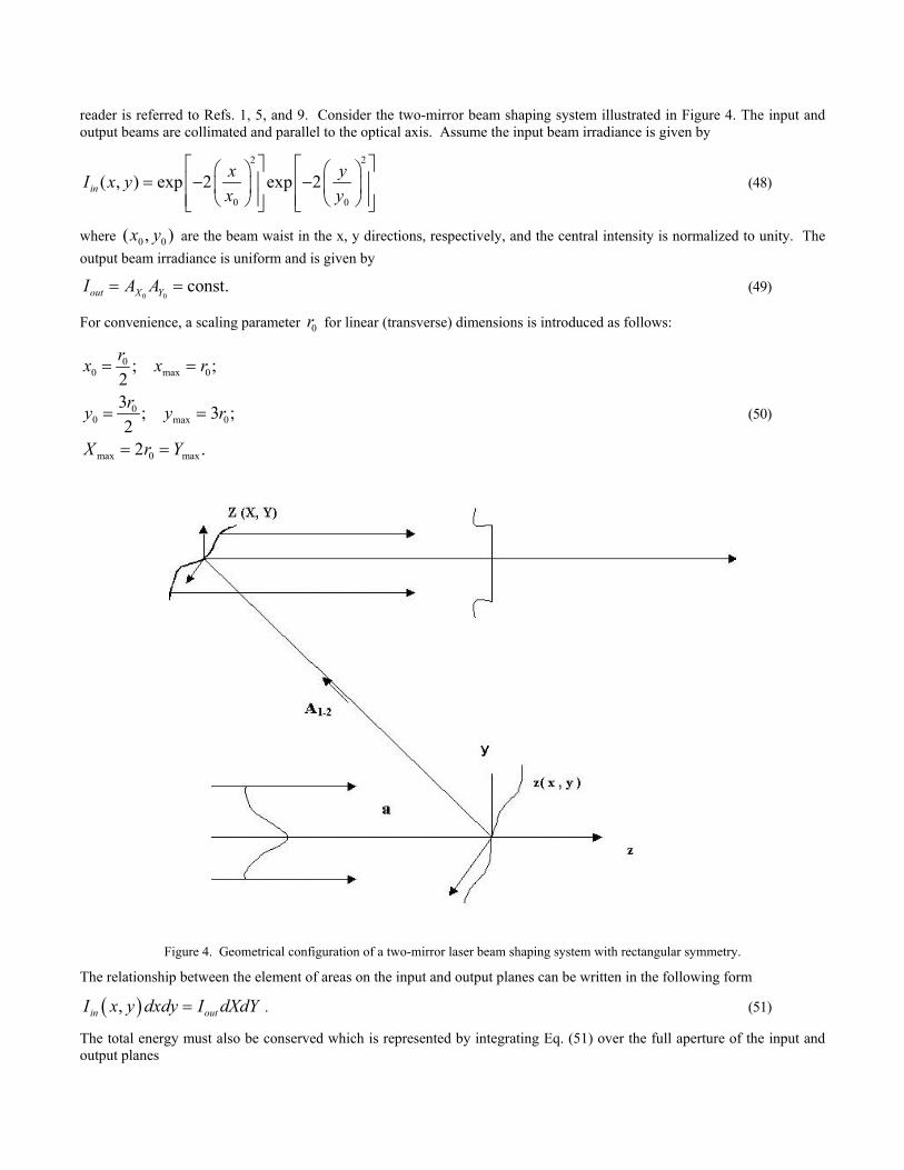
reader is referred to Refs. 1, 5, and 9. Consider the two-mirror beam shaping system illustrated in Figure 4. The input and output beams are collimated and parallel to the optical axis. Assume the input beam irradiance is given by

2 2

0 0

( , ) exp 2 exp 2inx yI x yx y

= − −

(48)

where 0 0( , )x y are the beam waist in the x, y directions, respectively, and the central intensity is normalized to unity. The output beam irradiance is uniform and is given by

0 0const.out X YI A A= = (49)

For convenience, a scaling parameter for linear (transverse) dimensions is introduced as follows: 0r

00 max

00 max

max 0 max

; ;23 ; 32

2 .

rx x r

ry y

X r Y

= =

= =

= =

0

0;r (50)

Figure 4. Geometrical configuration of a two-mirror laser beam shaping system with rectangular symmetry.

The relationship between the element of areas on the input and output planes can be written in the following form

( ),in outI x y dxdy I dXdY= . (51)

The total energy must also be conserved which is represented by integrating Eq. (51) over the full aperture of the input and output planes

max max max max

0

max max max max

2 2

0 0

exp 2 exp 2x y X

in X Yx y X

x yE dx dy A dXx y− − −

0

Y

Y

A dY−

= − − =

∫ ∫ ∫

∫ . (52)

or explicitly after evaluating the integrals

( ) ( ) 20 0in 0

2 3 2E = 2 2 2 2 164 4 out

r rerf erf I rπ π =

(53)

from which it follows that

( ) 23 2 2 0.07362175017128outI erfπ = = . (54)

For interesting applications, it is desirable to have a non-uniform shaping of the laser beam profile in orthogonal directions. Therefore, assume that there is an independent and non-uniform magnification of the x and y ray coordinates between the input and output planes:

X m xx= ( )x

y

, (55)

Y m y yy= b g . (56)

The rectangular magnifications can be determined by imposing the incremental expression of conservation of energy, Eq. (51), for the separated intensity functions, Eqs. (48) and (49).

m x m yx ( ) and b gUsing approach proposed by Ref. 9, the output irradiance expressions along the x, y directions are given by

(0

0

2

0 00

1 2 2exp 2 2 22 16

r

XxA dx

r rπ

= − =

∫ )erf , (57)

(0

0

23

0 00

1 2 3 2exp 2 2 22 3 16

r

YyA dy

r rπ

= − =

∫ )erf , (58)

and the output plane position coordinates X, Y are given by

( )0

20

000

2 21 2exp 2 2

2 2

x

X

xerfruX du r

A r erf

= − =

∫ (59)

( )0

20

000

2 231 2exp 2 2

3 2 2

y

Y

yerfrvY dv r

A r erf

= − =

∫ (60)

Equations (59) and (60) can be used to evaluate numerical tables relating ( ),x y to ( ),X Y , which can then be used to invert

numerically the magnification equations (55) and (56) so that one can express ( ),x y in terms of ( , )X Y when evaluating

( , )Z X Y in Eq. (78) below.

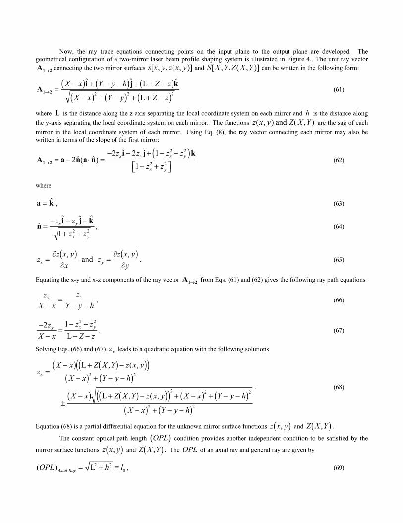
Now, the ray trace equations connecting points on the input plane to the output plane are developed. The geometrical configuration of a two-mirror laser beam profile shaping system is illustrated in Figure 4. The unit ray vector

connecting the two mirror surfaces and can be written in the following form: A1 2→ s x y z x y[ , , ( , )] S X Y Z X Y[ , , ( , )]

Ai j

1 2→ =− + − − + + −

− + − + + −

X x Y y h Z z

X x Y y Z z

b g b g bb g b g b g

L2 2 L

kg2

(61)

where is the distance along the z-axis separating the local coordinate system on each mirror and is the distance along the y-axis separating the local coordinate system on each mirror. The functions are the sag of each mirror in the local coordinate system of each mirror. Using Eq. (8), the ray vector connecting each mirror may also be written in terms of the slope of the first mirror:

L hY,z x y Z X( , ) ( )and

( )2 2

2 2

ˆ ˆ ˆ2 2 1ˆ ˆ2 ( )

1x y x y

x y

z z z zz z→

− − + − −= − ⋅ =

+ + 1 2

i j kA a n a n (62)

where

a k= , (63)

ni j

=− − +

+ +

z z

z zx y

x y1 2 2

k, (64)

zz x y

xz

z x yyx y=

∂∂

=∂∂

, ,b g b gand . (65)

Equating the x-y and x-z components of the ray vector from Eqs. (61) and (62) gives the following ray path equations A1 2→

zX x

zY y h

x y

−=

− −, (66)

−−

=− −+ −

2 1 2 2zX x

z zZ z

x x y

L. (67)

Solving Eqs. (66) and (67) leads to a quadratic equation with the following solutions zx

zX x Z X Y z x y

X x Y y h

X x Z X Y z x y X x Y y h

X x Y y h

x =− + −

− + − −

±− + − + − + − −

− + − −

b g b gc hd ib g b gb g b gc hd i b g b g

b g b g

L

L

, ( ,

, ( ,

2 2

2 2 2

2 2

. (68)

Equation (68) is a partial differential equation for the unknown mirror surface functions and . z x y,b g Z X Y,b g The constant optical path length b condition provides another independent condition to be satisfied by the

mirror surface functions and . The OPL of an axial ray and general ray are given by

OPLgY, gz x y,b g Z Xb

2 20( ) LAxial RayOPL h l= + ≡ , (69)

( ) ( ) ( ) ( )( ) (22 2 L , ( , ) ( , ) ,General Ray

OLP X x Y y h Z X Y z x y Z X Y z x y= − + − − + + − + − )

)

. (70)

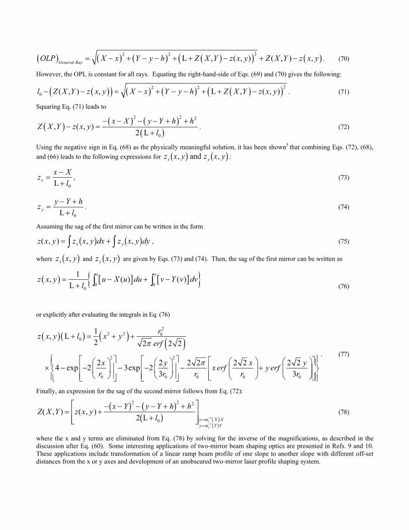
However, the OPL is constant for all rays. Equating the right-hand-side of Eqs. (69) and (70) gives the following:

( )( ) ( ) ( ) ( )( 22 20 ( , ) , L , ( , )l Z X Y z x y X x Y y h Z X Y z x y− − = − + − − + + − . (71)

Squaring Eq. (71) leads to

( ) ( ) ( )( )

2 2 2

0

, ( , )2 L

x X y Y hZ X Y z x y

l− − − − + +

− =+

h. (72)

Using the negative sign in Eq. (68) as the physically meaningful solution, it has been shown5 that combining Eqs. (72), (68), and (66) leads to the following expressions for : z x y z x yx y, ,b g b gand

z x Xlx =

−+L 0

, (73)

z y Y hly =

− ++L 0

. (74)

Assuming the sag of the first mirror can be written in the form

z x y z x y dx z x y dyx y( , ) , ,= + zz b g b g , (75)

where and are given by Eqs. (73) and (74). Then, the sag of the first mirror can be written as z x yx ,b g z x yy ,b g( ) [ ] [ ] 0 0

0

1, ( )L

x yz x y u X u du v Y v dv

l= − + −

+ ∫ ∫ ( ) (76)

or explicitly after evaluating the integrals in Eq. (76)

( ) ( ) ( ) ( )2

2 2 00

2 2

0 0 0 0

1, L2 2 2 2

2 2 2 2 2 2 2 24 exp 2 3exp 23 3

rz x y l x yerf

x y xx erf y erfr r r r

π

π

+ = + +

0

yr

× − − − − − +

. (77)

Finally, an expression for the sag of the second mirror follows from Eq. (72):

Z X Y z x yx Y y Y h h

l x m X Xy m Y Y

x

y

( , ) ( , )= +− − − − + +

+

LNMM

OQPP =

=

−

−

b g b gb g b g

b g

2 2 2

02 1

1L

(78)

where the x and y terms are eliminated from Eq. (78) by solving for the inverse of the magnifications, as described in the discussion after Eq. (60). Some interesting applications of two-mirror beam shaping optics are presented in Refs. 9 and 10. These applications include transformation of a linear ramp beam profile of one slope to another slope with different off-set distances from the x or y axes and development of an unobscured two-mirror laser profile shaping system.

4. SUMMARY AND CONCLUSIONS A geometrical optics theory for the design of laser beam shaping systems has been presented. This theory of laser beam shaping is based on conservation of radiant energy within a bundle of rays, which is also known as the intensity law for propagation of a bundle of rays, the ray trace equations, and the constant optical path length condition for cases when the contour of the incident wavefront is maintained as the beam passes through the system. This theory has been used to develop equations for the shapes of the optical surfaces for one-mirror, two-plano-aspheric lenses, and two-mirror beam shaping systems, that will transform a Gaussian input beam into a uniform irradiance output beam. Parametric equations, which define the contour of the two-mirror surfaces required to transform a Gaussian input beam with an elliptical cross-section into a circular output beam with uniform irradiance, are presented.

REFERENCES 1. D. L. Shealy, “Geometrical Methods,” in Laser Beam Shaping: Theory and Techniques, Marcel Dekker, Inc., New York, in print. 2. W.T. Silfvast, Laser Fundamentals, Cambridge University Press, New York, 1996. 3. J.H. McDermit and T.E. Horton, “Reflective optics for obtaining prescribed irradiative distributions from collimated sources,”

Applied Optics 13, pp. 1444-1450, 1974. 4. J.H. McDermit, Curved reflective surfaces for obtaining prescribed irradiation distributions, Ph.D. Dissertation, University of Mississippi,

Oxford, 1972. 5. P.W. Malyak, “Two-mirror unobscured optical system for reshaping the irradiance distribution of a laser beam,” Applied Optics 31, pp.

4377-4383, 1992. 6. J.L. Kreuzer, “Coherent light optical system yielding an output beam of desired intensity distribution at a desired equiphase surface,” U. S.

Patent 3,476,463, 4 November, 1969. 7. P.W. Rhodes and D.L. Shealy, “Refractive optical systems for irradiance redistribution of collimated radiation: their design and analysis,”

Applied Optics 19, pp. 3545-3553, 1980. 8. P.W. Rhodes, Design and analysis of refractive optical systems for irradiance redistribution of collimated radiation, M. S. Thesis, The

University of Alabama in Birmingham, 1979. 9. D. F. Cornwell, Non-projective transformations in optics, Ph.D. Dissertation, University of Miami, Coral Gables, 1980. 10. D. F. Cornwell, “Non-projective transformations in optics,” Proc. SPIE 294, pp. 62-72, 1981. 11. W. Jiang, D.L. Shealy, and J.C. Martin, “Design and testing of a refractive reshaping system,” Proc. SPIE 2000, pp. 64-75, 1993. 12. W. Jiang, Application of a laser beam profile reshaper to enhance performance of holographic projection systems, Ph.D. Dissertation, The

University of Alabama at Birmingham, 1993. 13. W. Jiang, D.L. Shealy, and K.M. Baker, “Optical design and testing of a holographic projection system,” Proc. SPIE 2152, pp. 244-252,

1994. 14. P. Mouroulis and J. Macdonald, Geometrical Optics and Optical Design, Oxford University Press, New York, 1997. 15. M. Born and E. Wolf, Principles of Optics, Fifth Edition, Pergamon Press, New York, 1975. 16. S. Solimeno, B. Crosignani, and P. DiPorto, Guiding, Diffraction, and Confinement of Optical Radiation, p. 49, Academic Press, Orlando,

1984. 17. A.K. Ghatak and K. Thyagarajan, Contemporary Optics, p. 24, Plenum Press, New York, 1980. 18. Born and Wolf, p. 115. 19. D.G. Koch, “Simplified Irradiance/Illuminance Calculations in Optical Systems,” presented at the International Symposium on Optical

Systems Design, Berlin, Germany, September 14, 1992, and published in Proc. SPIE 1780-14, 1992. 20. D.G. Burkhard, and D.L. Shealy, “Simplified formula for the illuminance in an optical system,” Applied Optics 20, pp. 897-909, 1981. 21. D.G. Burkhard and D.L. Shealy, “A Different Approach to Lighting and Imaging: Formulas for Flux Density, Exact Lens and Mirror

Equations and Caustic Surfaces in Terms of the Differential Geometry of Surfaces,” Proc. SPIE 692, pp. 248-272, 1986. 22. O.N. Stavroudis, The Optics of Rays, Wavefronts, and Caustics, pp. 82-84, Academic Press, New York, 1972. 23. Military Standardization Handbook - Optical Design, section 6.8, volume MIL-HDBK-141, Defense Supply Agency, Washington 25, DC, 5

October, 1962. 24. Stavroudis, Chapter II. 25. Silfvast, pp. 337-45. 26. CODE V is a registered trademark of Optical Research Associates, 3280 E. Foothill Blvd., Pasadena, CA 91107. 27. OSLO is a registered trademark of Sinclair Optics, Inc., 6780 Palmyra Road, Fairport, NY 14450. 28. ZEMAX is a registered trademark of Focus Software, Inc., P.O. Box 18228, Tucson, AZ 85731. 29. W.J. Smith and Genesee Optics Software, Inc., Modern Lens Design, p. 51, McGraw-Hill, New York , 1992. 30. A. Meddler and R. Mead, “A simplex method for function minimization,” Computer Journal 7, pp. 308, 1965. 31. N.C. Evans and D.L. Shealy, “Design and optimization of an irradiance profile shaping system with a genetic algorithm method,” Applied

Optics 37, pp. 5216-5221, 1998. 32. W. Jiang and D.L. Shealy, “Development and Testing of a Refractive Laser Beam Shaping System.” Proc. SPIE 4095-19, 2000.