Geometrical methods for Physics

Iberê Kuntz1 and Christopher Fritz2

Physics & Astronomy, University of Sussex

Falmer, Brighton, BN1 9QH, United Kingdom

1E-mail: ibere.kuntz@sussex.ac.uk2E-mail: c.fritz@sussex.ac.uk

Contents

I Geometry and Topology 3

1 Preliminaries 41.1 Maps and Sets . . . . . . . . . . . . . . . . . . . . . . . . . . . . . . . . . . 41.2 Morphisms . . . . . . . . . . . . . . . . . . . . . . . . . . . . . . . . . . . . 71.3 Topological spaces and manifolds . . . . . . . . . . . . . . . . . . . . . . . 81.4 Tensors . . . . . . . . . . . . . . . . . . . . . . . . . . . . . . . . . . . . . 10

2 Homotopy groups 142.1 Fundamental groups . . . . . . . . . . . . . . . . . . . . . . . . . . . . . . 142.2 Properties of the fundamental group . . . . . . . . . . . . . . . . . . . . . 162.3 Examples of fundamental groups . . . . . . . . . . . . . . . . . . . . . . . 17

3 Differential Topology 203.1 Charts and Coordinates . . . . . . . . . . . . . . . . . . . . . . . . . . . . 203.2 Functions and Curves . . . . . . . . . . . . . . . . . . . . . . . . . . . . . . 243.3 Vectors and One-forms . . . . . . . . . . . . . . . . . . . . . . . . . . . . . 263.4 Induced maps and Flows . . . . . . . . . . . . . . . . . . . . . . . . . . . . 283.5 Lie Derivatives and Brackets . . . . . . . . . . . . . . . . . . . . . . . . . . 323.6 Differential Forms and Tensors . . . . . . . . . . . . . . . . . . . . . . . . . 35

4 Differential Geometry 414.1 Metric . . . . . . . . . . . . . . . . . . . . . . . . . . . . . . . . . . . . . . 414.2 Connections . . . . . . . . . . . . . . . . . . . . . . . . . . . . . . . . . . . 454.3 Geodesics . . . . . . . . . . . . . . . . . . . . . . . . . . . . . . . . . . . . 504.4 Torsion and Curvature . . . . . . . . . . . . . . . . . . . . . . . . . . . . . 51

1

II Applications 53

5 General Relativity 545.1 Postulates . . . . . . . . . . . . . . . . . . . . . . . . . . . . . . . . . . . . 545.2 Tetrad formalism . . . . . . . . . . . . . . . . . . . . . . . . . . . . . . . . 555.3 Hodge Map . . . . . . . . . . . . . . . . . . . . . . . . . . . . . . . . . . . 595.4 Curvature and Torsion . . . . . . . . . . . . . . . . . . . . . . . . . . . . . 635.5 Electromagnetism and Einstein’s Equations . . . . . . . . . . . . . . . . . 64

6 Topological defects on condensed matter 676.1 Topological charges . . . . . . . . . . . . . . . . . . . . . . . . . . . . . . . 72

2

Part I

Geometry and Topology

3

Chapter 1

Preliminaries

In the present chapter we are going to introduce a few basic mathematical conceptsthat will be necessary in this course. We will discuss only briefly each new concept andwill stick mainly to the basic definitions, without proving anything in detail. The reasonfor this is that it would take a whole course to go through the theory underlying each ofthem. The good news is that we do not need the whole theory to start doing geometry.The only prerequisites for this chapter (and for the rest of course) are calculus and linearalgebra.

1.1 Maps and SetsFrom the point of view of a physicist, perhaps the most daunting aspect of differential

geometry is its comparative rigor and accompanying notation. So before diving headlonginto the subject, it might be worth spending the space of a chapter just elucidating someof the more basic concepts and notations that can make texts on differential geometryseem a bit alien. Hopefully it will become clear that this is simply another way of lookingat objects (like functions) which are already familiar, but allow for the concept to begeneralized.

If that seems a bit incoherent, let’s start by looking at an example. Take the function

f(x) = x2 + 5. (1.1)

Now what is this actually saying? Well if we insert some value x into our function, it isinstructing us to square that value and then add five. The result is another number, sowe could take x = 1 and get 6 or x = 5 and get 30. So what is actually happening hereis that the function f is assigning a number to each value of x (also a number). Since

4

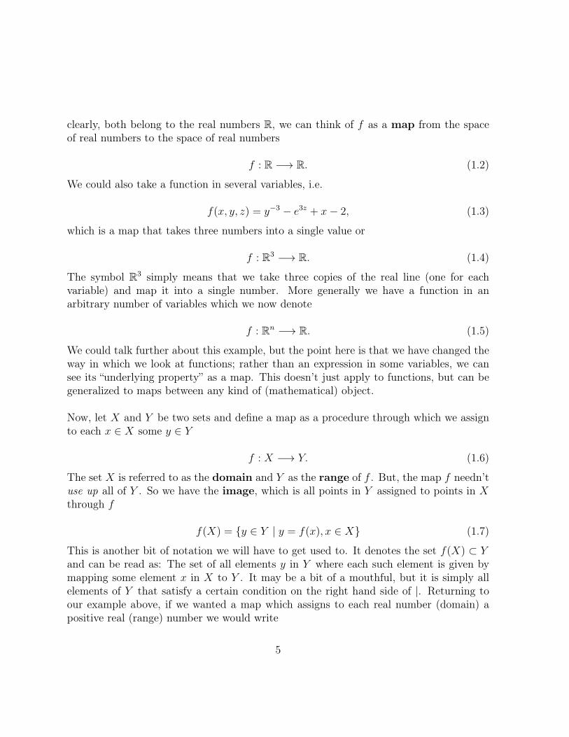
clearly, both belong to the real numbers R, we can think of f as a map from the spaceof real numbers to the space of real numbers

f : R −→ R. (1.2)

We could also take a function in several variables, i.e.

f(x, y, z) = y−3 − e3z + x− 2, (1.3)

which is a map that takes three numbers into a single value or

f : R3 −→ R. (1.4)

The symbol R3 simply means that we take three copies of the real line (one for eachvariable) and map it into a single number. More generally we have a function in anarbitrary number of variables which we now denote

f : Rn −→ R. (1.5)

We could talk further about this example, but the point here is that we have changed theway in which we look at functions; rather than an expression in some variables, we cansee its “underlying property” as a map. This doesn’t just apply to functions, but can begeneralized to maps between any kind of (mathematical) object.

Now, let X and Y be two sets and define a map as a procedure through which we assignto each x ∈ X some y ∈ Y

f : X −→ Y. (1.6)

The set X is referred to as the domain and Y as the range of f . But, the map f needn’tuse up all of Y . So we have the image, which is all points in Y assigned to points in Xthrough f

f(X) = y ∈ Y | y = f(x), x ∈ X (1.7)

This is another bit of notation we will have to get used to. It denotes the set f(X) ⊂ Yand can be read as: The set of all elements y in Y where each such element is given bymapping some element x in X to Y . It may be a bit of a mouthful, but it is simply allelements of Y that satisfy a certain condition on the right hand side of |. Returning toour example above, if we wanted a map which assigns to each real number (domain) apositive real (range) number we would write

5

f : R −→ R>0 (1.8)

and define the range as the set

R>0 = x ∈ R | x > 0 (1.9)

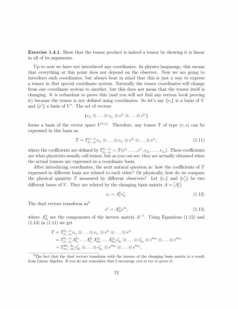
whose elements are strictly greater than zero. We will look at more examples shortly, butfirst let us consider some properties of maps. Firstly a map f : X −→ Y can have certainproperties (see Figure 1.1):

Figure 1.1: a) Injective function, b) surjective function and c) bijective function.

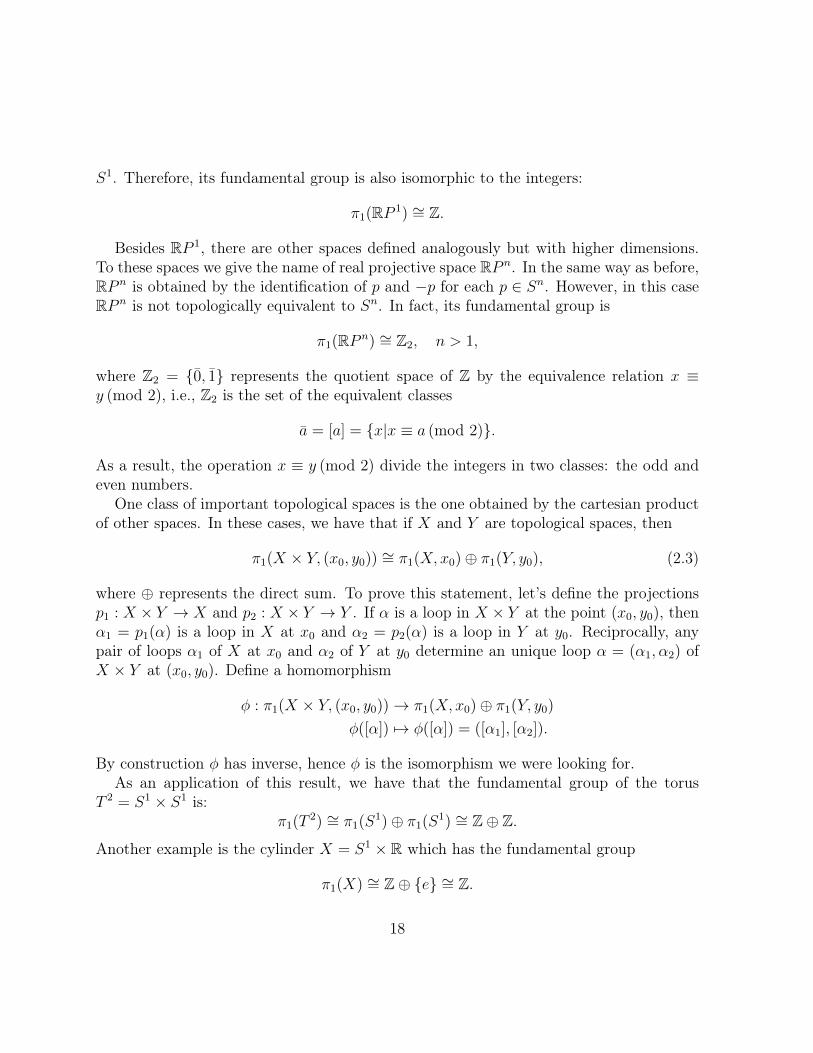
• Injective (or one-to-one): Each element in the domain maps to one and only oneelement of the range i.e. ∀x, x′ ∈ X if x 6= x′ then f(x) 6= f(x′).

• Surjective (or onto): Each element in the domain maps to at least one element ofthe range i.e. ∀y ∈ Y there exists at least one x ∈ X such that y = f(x).

• Bijective (one-to-one correspondence): Each element in the domain maps to oneand only one element of the entire range i.e. a map f is both injective and surjective.A map f has an inverse if and only if it is bijective.

Although a map needn’t be any of these. So, to take an example, if we let f :R → R and f(x) = cos(x), then this function is neither injective nor surjective: Sincecos(0) = cos(2π) = cos(4π) = · · · = 1, injectivity fails, and since cos(x) only takesvalues in the range from −1 to 1 so does surjectivity. However, we can define the setsX = x ∈ R | 0 ≤ x ≤ 2π and Y = x ∈ R | −1 ≤ x ≤ 1 and take these to be thedomain and range respectively. Now the map f : X −→ Y is bijective, so both surjectiveand injective.

6

Another important property is that maps can be composed: If we have f : X → Zand g : Z → Y then we also have a map h : X → Y given by the composition

h = g f. (1.10)

Which is instructing us to first apply f followed by g. Note that this only works if thedomain of g corresponds to the range of f . For example, consider f, g : R → R (whichmay be a bit reductive, but ought to illustrate the point) where this is clearly satisfiedand fix f, g to be the functions f(x) = cos(x) and g(x) = x2 − 1. Now we can find thecomposite function h = gf of some number x by h(x) = gf(x) = g(f(x)) = cos2(x)−1.

We also note the existence of inverse maps; that is for some f : X → Y there mayalso (but not necessarily) exist an inverse f−1 : Y → X. They can be composedf−1 f = f f−1 = id where id is the identity operator and simply maps elements ofa set back to themselves. So once again we take f : R → R as f(x) = cos(x) which alsogives us f−1 : R→ R as f−1(x) = cos−1(x) and f−1 f(x) = cos−1(cos(x)) = x.

1.2 MorphismsThe modern way to deal with mathematics is through structures. A mathematical

structure is to be viewed as some sort of relations imposed over a set of objects (thiscould be numbers, or matrices, or bananas, etc). A set A together with some structureΩ forms what we will call space and which will be denoted as an ordered pair (A,Ω).Essentially there are two types of structures: the algebraic structures and the geometricalones. How to define them and consequently classify all of the mathematical structuresin these two categories is not a trivial task, but this will not bother us here. In fact, inthis course we will only assume that a structure is algebraic whenever there is a product between the elements of the set A, denoted (A, ).

In this sense, the trend in mathematics is to isolate some structure from the rest and tryto understand everything about it, exhausting all of the possible definitions, theorems andso on. The way this usually happens is through the generalization of intuitive concepts.The idea of distance, for example, is very intuitive to all of us, but the mathematicianshave gone beyond that and have introduced a new structure called metric space, turningthe results we know from Euclidian space into axioms. This way we can get a deepunderstanding of what distance is without getting confused due to other concepts thatare also present in Euclidian space.

7

In order to better understand some structure, we have to know when two spaces areequivalent with respect to this structure. To this notion of equivalence we give the nameof morphism. More precisely, if A and B are two sets together with some structure, then amorphism between A and B is a map φ : A→ B which preserves the underlying structure.In the special case that φ has an inverse φ−1 : B → A that is also a morphism, we callφ an isomorphism. If there is an isomorphism between A and B, then A and B are saidto be isomorphic. When the structure is algebraic, a morphism φ : (A, )→ (B, ·) meansthat

φ(a b) = φ(a) · φ(b),

for every a, b ∈ A. In this case the word homomorphism is often used instead of morphism.

Example 1.2.1.

1. If A and B are sets with no structure, then any function f : A→ B is a morphism.If f is invertible, then it is an isomorphism.

2. If V and W are vector spaces, then any linear transformation T : V → W is ahomomorphism.

As we go ahead in this course we will find different structures and different types ofmorphisms with respect to it. Our job here is to study these structures and to identifythem in physics. By the way, this is essentially the role of mathematical physics.

1.3 Topological spaces and manifoldsOne the most important concepts in mathematics and that also appears everywhere in

physics is the idea of the continuum. We assume almost everywhere in physics that thefunctions are continuous, even though this is not always explicitly mentioned. The readermight be wondering right now how we could talk about continuity if the only thing wehave is a set of numbers. The answer is in another structure called topology1.

Definition 1. Let X be a set. A topology on X is a collection τ of subsets of X, calledopen sets, satisfying:

a) The entire set X and the empty set ∅ are open;1The word topology might refer to either the structure or the field/subject itself.

8

Figure 1.2: A map f : V → U . (a) f is continuous and the inverse image of U is open.(b) f is discontinuous and the inverse image of U is not open; V includes its end points.

b) The union of any family of open sets is open;

c) The intersection of any finite family of open subsets is open.

The pair (X, τ) is called a topological space. Whenever the topology τ is clear from thecontext, we will write X for the topological space.

Note that the notion of open sets was not defined previously and here they appearas mere objects belonging to a topological space. In topology, open sets are not definedindeed, but they are characterized by the rules of the above definition. This happensquite often in mathematics and for this reason we give these non-defined objects a name:primitive concepts. In summary we do not know what they are but we know how tooperate them. Likewise, vector is a primitive concept, so if you cannot accept open setsbecause they are not defined, always remember that you have been operating vectors sinceyour childhood.

Before we jump to continuity, here is an useful definition: a neighborhood of p ∈ Xis an open set containing p. Now we are able to talk about continuity. Let X and Y betopological spaces. A function F : X → Y is continuous if for every open set U ⊂ Ythe preimage F−1(U) is open in X. In other words, a continuous function is simply afunction which maps open sets into open sets in the reverse direction. This is the essenceof continuity (see the illustration in 1.2). When X = Y = R, it can be proved that thisdefinition reduces to that one you propably have seen in your calculus course.

Further, a map (in the sense of a function) has associated to it a so-called differentia-bility class denoted by Cn. This relates to its properties under differentiation so that, forexample, a continuous map whose first order derivative is also continuous, but where thesecond order isn’t, is in C1. All continuous maps are automatically in C0. All functionswhose kth order derivatives exist and are continuous, are in Ck. E.g. f(x) = |x|, whichis obviously in C0. However, its derivative f ′(x) = 1 if x > 0 and f ′(x) = −1 if x < 0 isnot continuous and hence is not an element of C1. Meanwhile, the function f(x) = |x|2

9

has first order derivative f ′(x) = |x| if x > 0 and f ′(x) = −|x| if x < 0 which is con-tinuous, but its second order derivative is not. Hence |x|2 is in C1. In general we have|x|n ∈ Cn−1. On the other hand, if a function is infinitely many times differentiable withall derivatives being continuous then it is in the special class C∞ and is called smooth.Examples include the ordinary exponential and trigonometric functions.

Since a continuous function maps open sets into open sets, it preserves the topologystructure. Therefore, continuous functions are the morphisms of topological spaces. Theisomorphisms in this context are called homeomorphisms (be careful, this is not the sameas the homomorphisms).

As you may have realized, topological spaces are very general spaces and this allowsus to obtain very general results as well. Unfortunately, on the other hand, they are sogeneral that they include some pathological cases that are not of our interest. As anexample, consider the topology τ = X, ∅ over X, formed by the entire set itself andthe empty set; this is called the trivial topology. In this case it can be proved that everysequence converges to every point of X and that every function into X is continuous.

To avoid these cases, which appears when X does not have enough subspaces, thefollowing additional axiom is often assumed. For every pair of different points p, q ∈ X,there exist disjoint open subsets U, V ⊂ X (i.e., U ∩ V ) such that p ∈ U and q ∈ V .Topological spaces that satisfy this axiom are called Hausdorff topological space or simplyHausdorff space.

A topological manifold M of dimension n is a Hausdorff topological space M which forevery point p ∈M there exists a neighborhood of p homeomorphic to an open set of Rn.Intuitively speaking, this means that every neighborhood of M looks like the usual realspace.

1.4 TensorsIt is impossible to overstress the usefulness of tensors for us. In mathematics they play

a very important role in a broad range of fields, specially in geometry. In physics theyappear everywhere as well, from moment of inertia to quantum field theory. Sadly tensorsare still poorly introduced in physics through its components and as objects defined bysome transformation. This leads to a lot of misconceptions and confusions. Here we willintroduce them in an abstract way, without using coordinates, and then show that whenwe pick up some coordinate frame we get the usual formulas used in the physics literature.

Before anything, it is important to be clear concerning notations. We are going to usesubscripts in vectors and superscript in coordinates of vectors whenever necessary. Onthe other hand, dual vectors will receive superscripts and its coordinates subscripts. In

10

addition, we will use Einstein notation when summing over indices, that is, we will sumover repeated indices and will omit the sum sign. So for example, in a basis ei a vectorwill be expressed as v = viei, while in a basis εj a dual vector will be expressed asω = ωjεj.

From linear algebra we know that a linear functional is a map T : V → R from a vectorspace V to the real numbers which satisfies linearity:

T (αu+ βv) = αT (u) + βT (v), α, β ∈ R u, v ∈ V.

Now let V1, . . . , Vn be vector spaces. A multilinear map is a map T : V1× . . .×Vn → Rwhich satisfies linearity in each of its components. Multilinear maps can also be addedand multiplied by scalars:

(aT + bS)(v1, . . . , vn) = aT (v1, . . . , vn) + bS(v1, . . . , vn).

Therefore, the set of all multilinear maps also forms a vector space itself, denoted

V ∗1 ⊗ . . .⊗ V ∗n

and called tensor product of dual spaces. Now let’s consider s copies of a vector space Vand r copies of its dual V ∗, that is,

T : V ∗ ⊗ . . .⊗ V ∗︸ ︷︷ ︸r times

⊗V ⊗ . . .⊗ V︸ ︷︷ ︸s times

→ R.

These multilinear maps are called tensors of type (r, s) on V . Since the dual of the dualspace V ∗∗ is isomorphic to V (prove it), the vector space of tensors can be written as

V (r,s) ≡ V ⊗ . . .⊗ V︸ ︷︷ ︸r times

⊗V ∗ ⊗ . . .⊗ V ∗︸ ︷︷ ︸s times

.

We usually set V (0,0) to be the real line R and hence the tensors in this case are scalars.For V (0,1) = V ∗ we have the usual linear functionals already found in linear algebra (alsocalled covectors) and for V (1,0) = V we have the ordinary vector space.

Let T and S be tensors of type (r, s) and (p, q) respectively. We define the tensorproduct between them as the tensor of type (r + p, s+ q) given by

T ⊗ S(ω1, . . . , ωr, ρ1, . . . , ρp, u1, . . . , us, v1, . . . , vq)

= T (ω1, . . . , ωr, u1, . . . , us)S(ρ1, . . . , ρp, v1, . . . , vq).

11

Exercise 1.4.1. Show that the tensor product is indeed a tensor by showing it is linearin all of its arguments.

Up to now we have not introduced any coordinates. In physics languange, this meansthat everything at this point does not depend on the observer. Now we are going tointroduce such coordinates, but always bear in mind that this is just a way to expressa tensor in that special coordinate system. Naturally the tensor coordinates will changefrom one coordinate system to another, but this does not mean that the tensor itself ischanging. It is redundant to prove this (and you will not find any serious book provingit) because the tensor is not defined using coordinates. So let’s say ei is a basis of Vand εj a basis of V ∗. The set of vectors

ei1 ⊗ . . .⊗ eir ⊗ εj1 ⊗ . . .⊗ εjs

forms a basis of the vector space V (r,s). Therefore, any tensor T of type (r, s) can beexpressed in this basis as

T = T i1...irj1...jsei1 ⊗ . . .⊗ eir ⊗ εj1 ⊗ . . .⊗ εjs , (1.11)

where the coefficients are defined by T i1...irj1...js= T (εi1 , . . . , εir , ej1 , . . . , ejs). These coefficients

are what physicists usually call tensor, but as you can see, they are actually obtained whenthe actual tensors are expressed in a coordinate basis.

After introducing coordinates, the next natural question is: how the coefficients of Texpressed in different basis are related to each other? Or physically, how do we comparethe physical quantity T measured by different observers? Let ei and e′j be twodifferent bases of V . They are related by the changing basis matrix A = [Aji ]:

ei = Aki e′k. (1.12)

The dual vectors transform as2

εj = A′jmεm, (1.13)

where A′jm are the components of the inverse matrix A−1. Using Equations (1.12) and(1.13) in (1.11) we get

T = T i1...irj1...jsei1 ⊗ . . .⊗ eir ⊗ εj1 ⊗ . . .⊗ εjs

= T i1...irj1...jsAk1i1 . . . A

krirA′j1m1

. . . A′j1mse′k1⊗ . . .⊗ e′kr ⊗ ε

′m1 ⊗ . . .⊗ ε′ms

= T ′k1...krm1...mse′k1 ⊗ . . .⊗ e

′kr ⊗ ε

′m1 ⊗ . . .⊗ ε′ms ,2The fact that the dual vectors transform with the inverse of the changing basis matrix is a result

from Linear Algebra. If you do not remember that I encourage you to try to prove it.

12

where the unprimed coefficients are the components of T with respect to the basis ei andthe primed ones are the components of T with respect to e′j. Therefore, the componentsof the tensor T transform as

T ′k1...krm1...ms= T i1...irj1...js

Ak1i1 . . . AkrirA′j1m1

. . . A′j1ms . (1.14)

And this is the “definition” of tensors one encounters in physics.

Example 1.4.1. We will see on Chapter 4 that a metric g is a tensor of type (0, 2). Soif εi is a basis for V ∗ we can write

g = gijεi ⊗ εj.

In this case, Equation 1.14 becomes

g′ij = gmnAmi A

nj .

13

Chapter 2

Homotopy groups

Mathematically, the classification of topological defects is done with the use of homo-topy groups, which are part of a huge mathematics field known as Algebraic Topology,whose aim is to use algebra to study topological problems.

Then naturally, before learning about the physics of topological defects, we have tointroduce some tools from the homotopy theory.

2.1 Fundamental groupsLet α : I = [0, 1] → X be a curve in X such that α(0) = α(1) = x0. Such curves

are called loops based at x0. It is possible to endow the set of all of these loops with analgebraic structure as follows.

Definition 2. Let α, β : I → X be loops such that α(1) = β(0). The product αβ isdefined as:

αβ(s) =

α(2s), 0 ≤ s ≤ 1

2,

β(2s− 1),1

2≤ s ≤ 1.

Geometrically, this definition corresponds to the curve obtained by traversing the imageof α and then the image of β. It is straightforward to show that the loop αβ is continuoussince α(1) = β(0).

To proceed with the construction of the algebraic structure, we also have to define theinverse and the identity elements. With the last definition in mind it is natural to defineα−1(s) = α(1− s), for each s ∈ I, which corresponds to traversing the loop α in the other

14

way around. Finally, the identity element is defined by cx(s) = x, i.e., the image cx(I) isa single point.

These definitions could suggest that α−1α = αα−1 = cx, however this is not true ascan be easily verified. To manage this problem we need the concept of homotopy.

Definition 3. A homotopy in x0 is a continous function h : I × I → X such that:

h0(s) = α(s), h1(s) = β(s), ∀s ∈ I, (2.1)ht(0) = ht(1) = x0, ∀t ∈ I, (2.2)

where α and β are loops based at x0. Then we say that there exists a homotopy between αand β based at x0, written α ∼ β. In this conditions, α and β are said to be homotopic.

In other words, two loops are homotopic if they can be continuously deformed to eachother.

Remarkably, the relation α ∼ β is an equivalence relation and its equivalence class[α] = β|α ∼ β is called the homotopic class of α. In fact, the relation ∼ satisfies theproperties:

- Reflexivity : α ∼ α. The homotopy can be given by ht(s) = α(s) for any ∈ I.- Symmetry : Let α ∼ β with the homotopy ht(s) such that h0(s) = α(s) and h1(s) =

β(s). Then β ∼ α, where the homotopy is given by h1−t(s).- Transitivity : Let α ∼ β and β ∼ γ. Then α ∼ γ. In fact, if ft(s) is a homotopy

between α and β and gt(s) is a homotopy between β and γ, a homotopy between α andγ can be given by

ht(s) =

f2t(s), 0 ≤ t ≤ 1

2

g2t−1(s),1

2< t ≤ 1.

Equipped with the set of homotopy classes at x, denoted by π1(X, x), and defining theoperation [α][β] = [αβ], we get the so called fundamental group. The fundamental groupis a group indeed, since it satisfies all of the axioms of a group:

- Associativity : A homotopy ft(s) between (αβ)γ and α(βγ) can be given by

ft(s) =

α

(4s

1 + t

), 0 ≤ s ≤ 1 + t

4,

β(4s− t− 1),1 + t

4< s ≤ 2 + t

4,

γ

(4s− t− 2

2− t

),

2 + t

4< s ≤ 1.

15

Therefore, we can simply write [αβγ] to denote [(αβ)γ] ou [α(βγ)].- Identity element : Define a homotopy as

ft(s) =

α

(2s

1 + t

), 0 ≤ s ≤ 1 + t

2,

x,1 + t

2< s ≤ 1.

Clearly this is a homotopy between αcx and α. Analogously, a homotopy between cxαand α is given by

ft(s) =

x, 0 ≤ s ≤ 1− t

2,

α

(2s− 1 + t

1 + t

),

1− t2

< s ≤ 1.

This show that [α][cx] = [cx][α] = [α].- Inverse: Define a homotopy ft(s) by

ht(s) =

α(2s(1− t)), 0 ≤ s ≤ 1

2,

α(2(1− s)(1− t)), 1

2< s ≤ 1.

Naturally, f0(s) = αα−1 and f1(s) = cx and, consequently,

[αα−1] = [α][α−1] = [cx].

This shows that [α−1] = [α]−1.Briefly, the fundamental group π1(X, x0) is the group formed by all of the homotopy

classes at x0, where [cx] is the identity element and, given [α], [α]−1 = [α−1] is its inverseelement.

2.2 Properties of the fundamental groupIn this section some of the most important properties of the fundamental group will

be presented. It is worth noting that the fundamental group was built considering verybroad conditions. Nonetheless, if we restrict our attention to some more specific cases(but still general enough to have an enormous applicability) we could be able to proveinteresting properties.

16

In this sense, consider a path connected topological space X (i.e., a space which anytwo points x0, x1 ∈ X can be connected by a continuous curve α such that α(0) = x0 andα(1) = x1). It is possible to show that there exists an isomorphism between π1(X, x0)and π1(X, x1). The proof is out of the scope of this course and can be found in anyintroductory book about homotopy. With this result, we can omit the base point of thehomotopy in path connected spaces and simply write π1(X).

The homotopy of loops can be easily generalized to continuous functions. Let X, Ybe topological spaces and f, g : X → Y be continuous functions. If there exists anothercontinuous function F : X× I → Y such that F (x, 0) = f(x) and F (x, 1) = g(x), then wesay that f is homotopic to g and we denote f ∼ g. The function F is called the homotopybetween f and g.

Two topological spaces X and Y are of the same homotopy type, denoted X ' Y , ifthere are continuous functions f : X → Y and g : Y → X such that f g ∼ idY andg f ∼ idX . The function f is called homotopy equivalence and g is its inverse.

Now it is possible to state one of the most important properties of this section: iff : X → Y is a homotopy equivalence between X and Y , π1(X, x0) is isomorphic toπ1(Y, f(x0)). As a colorary we have that the fundamental group is invariant under home-omorphisms, i.e., it is a topological invariant.

In this sense, fundamental groups classify topological spaces in a less restrict way thanhomeomorphisms do. Nevertheless, it is necessary to emphasize that fundamental groupsare used in physics to classify maps and field configurations instead of topological spaces.

2.3 Examples of fundamental groupsAlthough there are no systematic procedure to calculate the fundamental group, it is

possible to find it in some specific cases through some simple considerations.In the case of a circumference S1 the fundamental group is isomorphic to the integers;

π1(X) ∼= Z. Although the proof of this claim is not so obvious (see [B9]), its outcome canbe easily understood. Let’s supose that we encircle a cylinder with an elastic band. If theelastic band encircles the cylinder n times, then this configuration cannot be continuouslydeformed in another which encircles the cylinder m 6= n times. Moreover, if the elasticband encircles the cylinder n times and then m times, it encircles the cylinder n+m timesin total.

Another interesting topological space is the real projective line RP 1 which is the topo-logical space made through the identification of the points of a circumference to its respec-tive antipodes. This space can be thought of as the semicircle with indentified ends. Forthis reason, the real projective line RP 1 is topologically equivalent to the circumference

17

S1. Therefore, its fundamental group is also isomorphic to the integers:

π1(RP 1) ∼= Z.

Besides RP 1, there are other spaces defined analogously but with higher dimensions.To these spaces we give the name of real projective space RP n. In the same way as before,RP n is obtained by the identification of p and −p for each p ∈ Sn. However, in this caseRP n is not topologically equivalent to Sn. In fact, its fundamental group is

π1(RP n) ∼= Z2, n > 1,

where Z2 = 0, 1 represents the quotient space of Z by the equivalence relation x ≡y (mod 2), i.e., Z2 is the set of the equivalent classes

a = [a] = x|x ≡ a (mod 2).

As a result, the operation x ≡ y (mod 2) divide the integers in two classes: the odd andeven numbers.

One class of important topological spaces is the one obtained by the cartesian productof other spaces. In these cases, we have that if X and Y are topological spaces, then

π1(X × Y, (x0, y0)) ∼= π1(X, x0)⊕ π1(Y, y0), (2.3)

where ⊕ represents the direct sum. To prove this statement, let’s define the projectionsp1 : X × Y → X and p2 : X × Y → Y . If α is a loop in X × Y at the point (x0, y0), thenα1 = p1(α) is a loop in X at x0 and α2 = p2(α) is a loop in Y at y0. Reciprocally, anypair of loops α1 of X at x0 and α2 of Y at y0 determine an unique loop α = (α1, α2) ofX × Y at (x0, y0). Define a homomorphism

φ : π1(X × Y, (x0, y0))→ π1(X, x0)⊕ π1(Y, y0)φ([α]) 7→ φ([α]) = ([α1], [α2]).

By construction φ has inverse, hence φ is the isomorphism we were looking for.As an application of this result, we have that the fundamental group of the torus

T 2 = S1 × S1 is:π1(T

2) ∼= π1(S1)⊕ π1(S1) ∼= Z⊕ Z.

Another example is the cylinder X = S1 × R which has the fundamental group

π1(X) ∼= Z⊕ e ∼= Z.

18

Up to this point we have seen the basics about homotopy to start doing physics.We could go further and generalize all of this to higher dimensions. To do so, insteadof considering the fundamental group π1(X), we would define the nth homotopy groupπn(X) as the group that classifies n-loops α : In → X, where In denotes the n-cubeI × · · ·× I. For n = 2, for example, π2(X) would classify the homotopy classes of spheresin X. As our goal here is not to explain the whole theory of homotopy in detail, we leavesome good references for the interested reader [A1,B9].

19

Chapter 3

Differential Topology

3.1 Charts and CoordinatesThe notion of a topological space ought to be clear and is the starting point to define

smooth manifolds. If what we want to do is study physics, which we take to mean themotions of particles, simply specifying a topology doesn’t get us very far. In order tointroduce and generalize such things as velocity and acceleration, we need some sort ofdifferential structure, that is to say we need to figure out how to translate our usual flatspace calculus to some arbitrary curved space. A manifold is a type of topology thatin the neighborhood of each point looks like Euclidean (or in physics Minkowski) space.This is an extremely important property as it will allow us to endow our space a so-calledcoordinate chart which gives us access to the differential structure and apply our nor-mal calculus developed in flat space. Why is this important? Conventionally, we are usedto being able to visualize (so essentially to draw pictures of) the physical process we areinterested in. What this equates to is being able to frame quantities like momentum andposition relative to some coordinate axis (so we can specify everything in terms of x,yand z (and possibly t) coordinates). And indeed, we know that at a given scale, we candescribe everything in terms of this simple 3D Euclidean (or 4D Minkowski) coordinatesystem. This may sound familiar as the equivalence principle in GR. What this means isthat any space can be considered to be flat at small enough scales, or to put it differently,every space looks locally Euclidean (or Minkowski). Another important aspect, is thatthis gives us a notions of calculus on a manifold since it is, at these sufficiently smallscales, simply the same calculus we are familiar with (that is, the calculus of Rn).

20

However, a manifold1 isn’t simply isomorphic to Rn. Rather, we use something calledan Atlas which is a set of pairs (Ui, ψi). We denote byM a topological space which iscalled a manifold if it has

• Ui an open subset Ui ⊆ M which satisfies⋃i

Ui = M. So the union of all subsets

cover the entire manifold

• ψi a homeomorphism into an open subset of Rn so that ψi : Ui → ψ(Ui) ⊆ Rn

• Given a nonempty intersection Ui∩Uj 6= ∅, there exists a transition function φij :Rn → Rn or, more precisely φij : ψi(Ui∩Uj)→ ψj(Ui∩Uj), given by φij = ψi ψ−1j .φij which is also a homeomorphism.

See the illustration in (3.1). So, if we take a point on an m-dimensional manifold p ∈ Ui ⊆M, a map ψi assigns m coordinate values xµ where 1 ≤ µ ≤ m . So think of labelingeach point with coordinates (x, y, z · · · ). Meanwhile if p ∈ Ui ∩ Uj, ψi assigns xµ andψj assigns yν where 1 ≤ µ, ν ≤ m, the transition functions relating x to y are functionsin m variables of the form xµ = xµ(y). Moreover, for physics there are particular classesof manifolds that are interesting

• Differential Manifold: A manifold whose Atlases are equipped with transitionfunctions that are differentiable i.e. φ ∈ Ck

• Smooth Manifold: Same as a differential manifold, but the transition functionsare smooth: φ ∈ C∞

We will be concentrating on the latter since all examples we will encounter here aregoing to be of smooth manifolds. Let’s illustrate this by looking at a more heuristic ex-ample: the two sphere - S2.

We take S2 with unit radius embedded in R3 where points are labeled by (x, y, z). Asphere is denoted as S2 = (x, y, z) ∈ R3 | x2 + y2 + z2 = 1 so all points equidistant fromthe origin (0, 0, 0). Now, since the sphere is a two dimensional surface, we want a mapinto R2, where points are labeled as (X, Y ), so that we need φi : S2 → R2, a functiontaking points on the sphere to the plane. There are many different ways of doing this;

1Along the rest of this chapter manifolds will mean differentiable/smooth manifolds. Do not getconfused with the more general notion of a topological manifold introduced in Chapter 1.

21

Figure 3.1: Illustration of an Atlas: The charts ψ1 and ψ2 map the open subsets U1 andU2 into Rm and Rn. In the nonempty intersection U1 ∩ U2 one has transition functionsφ12 = φ−121 between charts.

one is so-called stereographic projection (see 3.2). We take the plane to lie at the height ofthe sphere’s equator perpendicular to the z-axis and project from the north pole (0, 0, 1),denoting this map ψN which relates points as

X =x

1− z, Y =

y

1− z. (3.1)

Notice however, ψN is not well defined at the north pole where z = 1. That means ouropen set UN cannot be all of S2, but rather must be a subset excluding that point. So wehave a set UN = S2−north pole. To cover the entire sphere, we need at least one moreopen set 2 which includes the north pole. A simple choice is the south pole at (0, 0,−1),though we could choose any other as long as it results in a chart which includes (0, 0, 1).Similar to before this gives a set US = S2 − north pole with chart

X ′ =x

1 + z, Y ′ =

y

1 + z, (3.2)

covering all of the sphere except the south pole. In summary we have two projectivecharts on the sphere mapping into the subsets

2In fact, a two sphere can never be coordinated by less than two charts. If it could, it would behomeomorphic to (i.e. the same as) the plane.

22

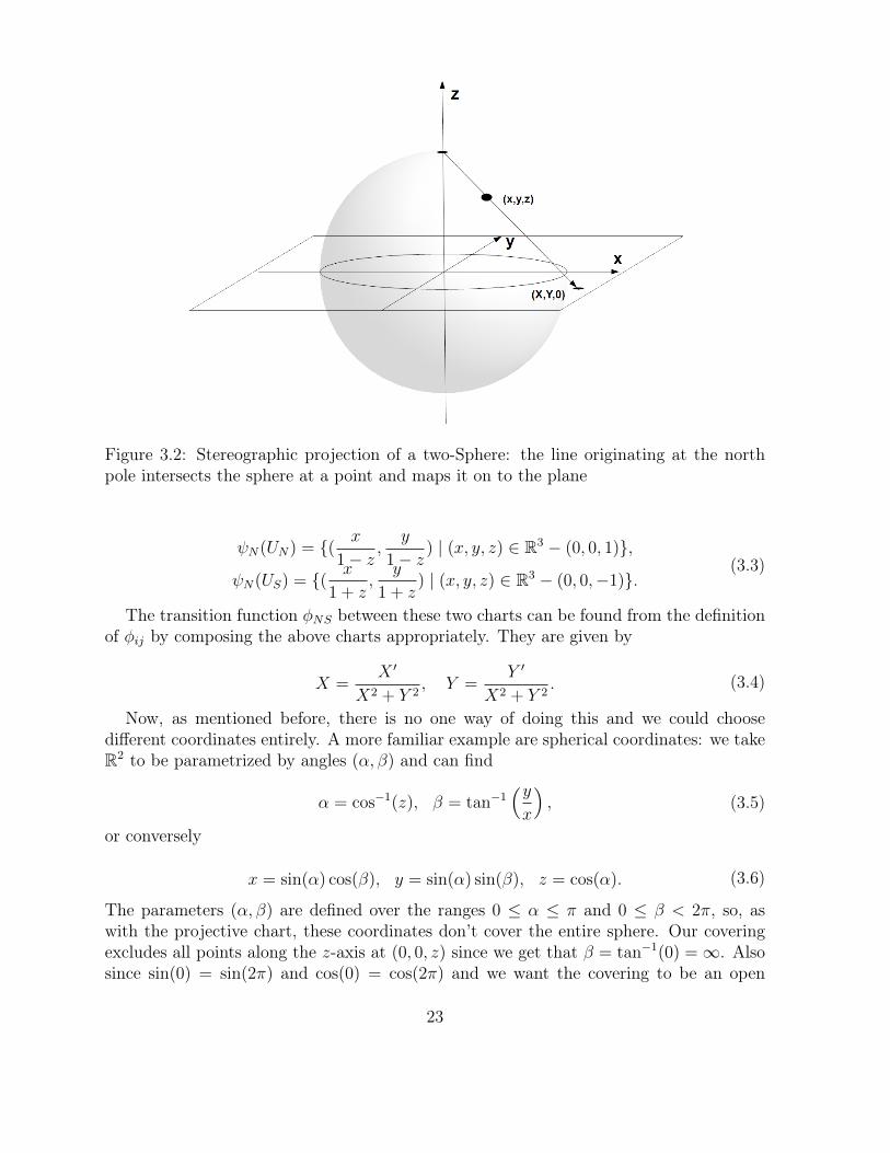
Figure 3.2: Stereographic projection of a two-Sphere: the line originating at the northpole intersects the sphere at a point and maps it on to the plane

ψN(UN) = ( x

1− z,

y

1− z) | (x, y, z) ∈ R3 − (0, 0, 1),

ψN(US) = ( x

1 + z,

y

1 + z) | (x, y, z) ∈ R3 − (0, 0,−1).

(3.3)

The transition function φNS between these two charts can be found from the definitionof φij by composing the above charts appropriately. They are given by

X =X ′

X2 + Y 2, Y =

Y ′

X2 + Y 2. (3.4)

Now, as mentioned before, there is no one way of doing this and we could choosedifferent coordinates entirely. A more familiar example are spherical coordinates: we takeR2 to be parametrized by angles (α, β) and can find

α = cos−1(z), β = tan−1(yx

), (3.5)

or conversely

x = sin(α) cos(β), y = sin(α) sin(β), z = cos(α). (3.6)

The parameters (α, β) are defined over the ranges 0 ≤ α ≤ π and 0 ≤ β < 2π, so, aswith the projective chart, these coordinates don’t cover the entire sphere. Our coveringexcludes all points along the z-axis at (0, 0, z) since we get that β = tan−1(0) =∞. Alsosince sin(0) = sin(2π) and cos(0) = cos(2π) and we want the covering to be an open

23

set, we exclude β = 2π. The end result is a single chart which covers the sphere exceptfor the poles and the great circle section connecting them. One could think of taking aninflatable ball, cutting it open along one side and flattening it out. More coverings ofthe entire sphere using this parametrization could be found by taking (α+ δ, β + γ). Wecan also find transition functions between our polar coordinates and stereographic ones.These are given by (for ψN)

X = cot(α

2

)cos(β), Y = cot

(α2

)sin(β). (3.7)

So we have at least two completely different coordinate systems for the sphere, thoughthere are many more. An everyday example of this, which also neatly demonstrates thedifficulties with choosing an appropriate mapping, can be found in every Atlas (the bookin this case). Earth, being (almost) a sphere, needs to be mapped into plane in order toproduce a map that can be drawn on a flat piece of paper. The most familiar one is theso-called Mercator projection. This has the drawback of hugely distorting the relativeproportions of landmasses the closer they are to the poles. For example, Greenlandlooks to be larger than Africa, though in actual fact the latter is about 14 times larger.Alternatives include the Gall-Peters and Dymaxion maps, the latter being a projectionfirst onto a polygon (Icosahedron) and then into the plane.

You have hopefully realized that everything we have been doing here is simply anexample of coordinate transformations. Different charts are simply different coordinatesystems and the statement that they all parametrize the same topology, albeit in differentranges, is an idea of central importance in general relativity. What we have done is tohopefully give some different intuition for something that is already quite familiar.

3.2 Functions and CurvesNow we have established what a manifold is, the next thing is to begin to look at the

structures it can possess e.g. functions, vector fields, tensors etc. Or to put it anotherway, how can one realize objects that are useful in physics within this formalism. Tobegin with, we briefly return to maps, but now specifically maps between manifolds.

So, let’s take f : M → N , where M and N are manifolds of dimension m and nrespectively and a point p ∈M is mapped to a point f(p) ∈ N . With a coordinate chart(U, ψ) on M and (V, θ) on N such that p ∈ U and f(p) ∈ V , f is assigned a coordinaterepresentation by the composition

θ f ψ−1 : Rm → Rn. (3.8)

24

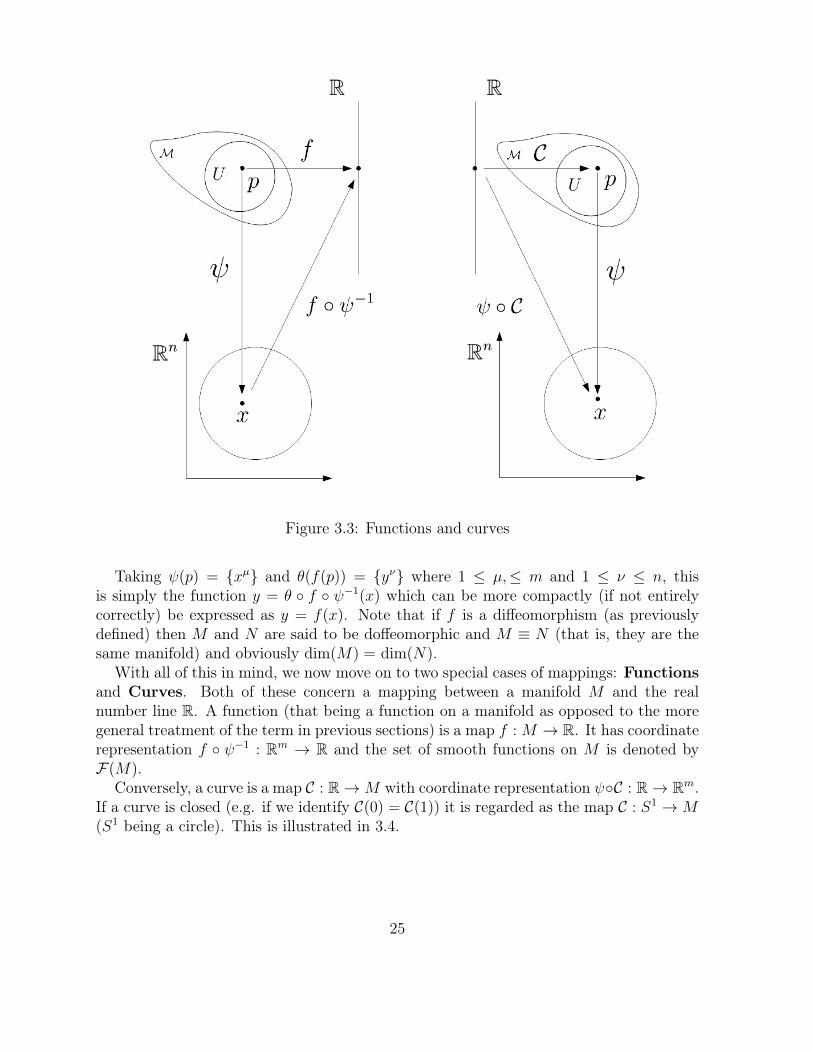
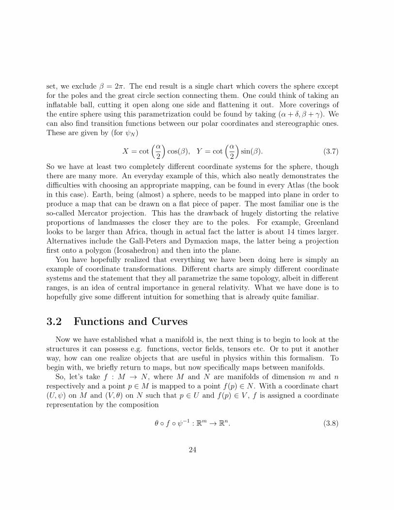
Figure 3.3: Functions and curves

Taking ψ(p) = xµ and θ(f(p)) = yν where 1 ≤ µ,≤ m and 1 ≤ ν ≤ n, thisis simply the function y = θ f ψ−1(x) which can be more compactly (if not entirelycorrectly) be expressed as y = f(x). Note that if f is a diffeomorphism (as previouslydefined) then M and N are said to be doffeomorphic and M ≡ N (that is, they are thesame manifold) and obviously dim(M) = dim(N).

With all of this in mind, we now move on to two special cases of mappings: Functionsand Curves. Both of these concern a mapping between a manifold M and the realnumber line R. A function (that being a function on a manifold as opposed to the moregeneral treatment of the term in previous sections) is a map f : M → R. It has coordinaterepresentation f ψ−1 : Rm → R and the set of smooth functions on M is denoted byF(M).

Conversely, a curve is a map C : R→M with coordinate representation ψC : R→ Rm.If a curve is closed (e.g. if we identify C(0) = C(1)) it is regarded as the map C : S1 →M(S1 being a circle). This is illustrated in 3.4.

25

3.3 Vectors and One-formsWe are now in a position to look at some more interesting objects. One may question

the purpose of the previous section, until the difficulties in defining something like a vectorbecome apparent. We are used to the notion of a vector as a straight arrow, but how isthis concept translated to a manifold? Where is the origin? What does it even mean forsomething to be ’straight’? So, we define a vector using both a function and a curve - itwill be a tangent vector. You will hopefully remember that the derivative of a functionis always tangent to that function. Let’s take two curves C1, C2 : R → M and λ ∈ R aparameter along the curves so that, for a point p ∈M , we have p = C1(0) = C2(0). Then,C1 and C2 are said to be tangent if and only if

dxµ(C1(λ))

dλ

∣∣∣∣λ=0

=dxν(C2(λ))

dλ

∣∣∣∣λ=0

. (3.9)

Note that while this does use a coordinate chart, if two curves are not tangent in aparticular chart, they won’t be in any intersecting chart. A tangent vector at a point p isthen the collection of all curves for which the above is satisfied. Formally referred to asan equivalence class, as a set it is expressed as

[C] =

C(λ) | Ci(0) = Cj(0) and

dxµ(Ci(λ))

dλ

∣∣∣∣λ=0

=dxν(Cj(λ))

dλ

∣∣∣∣λ=0

,∀i, j. (3.10)

So let’s be more explicit. Take a curve C : R→M parametrized once again by λ and afunction f : M → R. Then find the derivative of the function along the curve and expressthis in local coordinates

df(C(λ))

dλ

∣∣∣∣λ=0

=df

dxµdxµ(C(λ))

dλ

∣∣∣∣λ=0

. (3.11)

That is, we can find the derivative of a function f(C(λ)) at a point λ = 0 by applying anoperator

X = Xµ d

dxµ. (3.12)

In other words

X[f ] = Xµ df

dxµ=df(C(λ))

dλ

∣∣∣∣λ=0

. (3.13)

26

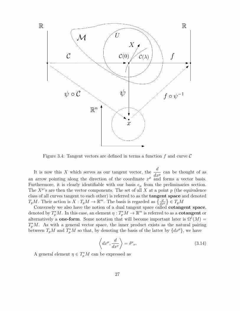
Figure 3.4: Tangent vectors are defined in terms a function f and curve C

It is now this X which serves as our tangent vector, thed

dxµcan be thought of as

an arrow pointing along the direction of the coordinate xµ and forms a vector basis.Furthermore, it is clearly identifiable with our basis eµ from the preliminaries section.The Xµ’s are then the vector components. The set of all X at a point p (the equivalenceclass of all curves tangent to each other) is referred to as the tangent space and denotedTpM . Their action is X : TpM → Rm. The basis is regarded as

ddxµ

∈ TpM

Conversely we also have the notion of a dual tangent space called cotangent space,denoted by T ∗pM . In this case, an element η : T ∗pM → Rm is referred to as a cotangent oralternatively a one-form. Some notation that will become important later is Ω1(M) =T ∗pM . As with a general vector space, the inner product exists as the natural pairingbetween TpM and T ∗pM so that, by denoting the basis of the latter by dxµ, we have⟨

dxµ,d

dxν

⟩= δµν . (3.14)

A general element η ∈ T ∗pM can be expressed as

27

η = ηµdxµ. (3.15)

Lastly, let’s take p ∈ Ui ∩Uj with charts assigning xµ and yν respectively. Then avector V ∈ TpM can be expanded as both

V = V µ ∂

∂xµ= V ν ∂

∂yν. (3.16)

So that they are related as

V µ = V ν ∂xµ

∂yν. (3.17)

The vector transforms so that V itself is invariant. Similarly for η ∈ T ∗pM

η = ηµdxµ = ηνdy

ν , (3.18)

so the relation is

ηµ = ην∂yν

∂xµ. (3.19)

A quick note on notation: Reading the preceding sections carefully ought to makeexpressions like ∂f

∂xµlook somewhat strange. That is because this is strictly speaking, an

abuse of notation and we ought to be using

∂

∂xµ(f ψ−1(x)

)(3.20)

instead (since the coordinate representation of a function depends on ψ). However, forthe sake of clarity, we will be sticking to the ’abuse of notation’ used in this chapter as itis the more familiar and compact.

3.4 Induced maps and FlowsNow that we have seen some of the structures interesting to physics emerging, we

might perhaps take some time to examine how they are manipulated. But first, wereturn, once again, to maps. Having introduced tangent spaces, we now need to examinetheir properties under mapping also. This is important since, by definition, TpM existsonly at a point and is distinct from Tp′M , the tangent space at any other point. So,it stands to reason that we somehow need to relate them. Let’s take another look at a

28

Figure 3.5: The map f : M → N induces the map f∗ : TpM → TpN on the tangentspace

smooth map f : M → N between two manifolds, recalling that it maps points p ∈ M tof(p) ∈ N . What this does, is to give us an induced map which we will denote

f∗ : TpM → Tf(p)M, (3.21)

acting on the tangent space. That is to mean, if we have some smooth map acting onpoints on the manifold, it induces a map acting on the vectors that live at those points.Explicitly, taking a vector V ∈ TpM and denoting its action on some function by V [g],we get

f∗V [g ψ−1(y)] = V [f g ψ−1(x)] (3.22)

in two coordinate charts on M and N . Ok, let’s try to be even more explicit and taketwo vectors V ∈ TpM and W ∈ Tf(p)N which are related by f∗(V ) = W . Both can be

expanded in a coordinate basis as V = V µ ∂

∂xµand W = W µ ∂

∂yµ. Then, taking g = xµ

(a coordinate function) and f : xµ → yµ, we get

V [xµ] = V α ∂xµ

∂xα= V µ (3.23)

and define our mapping so that

(f∗V )[xµ] = W [xµ(y)] = Wα∂xµ(y)

∂yα. (3.24)

So that we can relate the components as

V µ = Wα∂xµ(y)

∂yα, (3.25)

which hopefully looks familiar as a coordinate transformation. This juxtaposes before,where we showed that a coordinate transformation was to be thought of changing charts.

29

That, in fact, is what is called a passive coordinate transformation whereas whatwe just derived is an active coordinate transformation. To illustrate this let’s takeour example from before - the sphere S2 - and apply this. We look at our projectivecoordinate chart for the north pole and realize it as a map from R3 onto our sphere inR2, so f : R3 → S2 ⊂ R2 so that

f : (x, y, z)→ (X, Y ) = (x

1− z,

y

1− z). (3.26)

Now take some vector V ∈ TpR3 as V = a∂

∂x+ b

∂

∂y+ c

∂

∂zat some point p = (x, y, z) and

map it to f∗V ∈ Tf(p)R2. Then, applying this map

f∗V = V ν ∂yµ

∂xν∂

∂yµ

= a

(∂X

∂x+∂X

∂y+∂X

∂z

)∂

∂X+ b

(∂Y

∂x+∂Y

∂y+∂Y

∂z

)∂

∂Y

= a1− z − x(1− z)2

∂

∂X+ b

1− z − y(1− z)2

∂

∂Y

(3.27)

Alternatively, we could also take

f : (x, y, z)→ (α, β) = (cos−1(z), tan−1(yx

)), (3.28)

giving

f∗V = V ν ∂yµ

∂xν∂

∂yµ

= a

(∂α

∂x+∂α

∂y+∂α

∂z

)∂

∂α+ b

(∂β

∂x+∂β

∂y+∂β

∂z

)∂

∂β

= −a 1√1− z2

∂

∂α+ b

x− yx2 + y2

∂

∂β.

(3.29)

To compliment the above, we also have a second map acting on the dual tangent spacef ∗ : T ∗f(p)M → T ∗pM . The action of this map, taking one forms η : T ∗pM and ε : T ∗f(p)Mand identifying as beforef∗(η) = ε, is, in components

εµ =∂xµ

∂yνην . (3.30)

Note that it acts in the opposite direction of f∗. This directionality does in fact, lendnames to the maps: f∗ is called pushforward and f ∗ pullback.

30

Figure 3.6: Some properties of the flow σ induced by a vector field V

The next concept we want to tackle is that of flow, since it will lead us into the subjectof the next chapter. Take a curve C : R → M in some coordinate chart and a vectorV ∈ TxM (for simplicity we will denote both the point on the manifold and its coordinaterepresentation as x). Now write

d

dλ=dxµ

dλ

∂

∂xµ, (3.31)

so we are dealing with the tangent to that curve in a coordinate chart. For the vectorwrite

V [xν(λ)] = V µ ∂

∂xµxν(λ). (3.32)

Now, an integral curve, is a curve x(λ) whose tangent vector at a point xν(λ) is V |x.So using the above equations we can write

V µ(x(λ)) =d

dλxµ(λ). (3.33)

The solutions to this equation are denoted by σ(λ, x0) where x0 corresponds to thecoordinates of the point along the integral curve where λ = 0. This translates to theinitial condition

σµ(0, x0) = x0, (3.34)

and the above is written

V µ(σµ(λ, x0)) =d

dλσµ(λ, x0). (3.35)

31

We also have some of its properties illustrated in (3.6). This map is referred to as theflow generated by a vector field V .

3.5 Lie Derivatives and BracketsNow we are ready to look at some more interesting structures. It seems to be fact that

many people struggle with the intuition behind Lie Derivatives. Hopefully, this sectionwill show that as a concept these aren’t so nebulous as many suppose them to be andthat there is in fact, very simple intuition behind them.

To start with, let us take two vector fields V and W and their flows τ(λ, x) and σ(λ, x)so that we have

V µ =d

dλτµ(λ, x), W µ =

d

dλσµ(λ, x). (3.36)

Now let’s ask (and pay attention here), if we took a vector V at a point p somewhereon the integral curve generated by W (so σµ(λ, p)) and then ’pushed’ it along the curvesome distance ε (so to σµ(λ + ε, p)), how would V change? This is exactly what we aretrying to answer using the Lie Derivative and is illustrated in (3.8). For simplicity wewill speak of a single vector V , though this should of course always be vector field alsowe will suppress most of the information in σµ(λ + ε, p′) so that this becomes σε to saveon notation (and since we are only interested in the displacement). But we must bear inmind that vectors at different points on the manifold also live in different tangent spaces.So we use what we learned about induced maps in the previous section: To comparevectors that reside at different points, we must compare one to the pullback of the other.In this case, the map we are using is the flow and as you might imagine, the flow from pto σε(p) induces a pull back on the tangent space so σ∗−ε : Tσε(p) → Tp. The Lie derivativeof V along W is thus defined by

LWV = limε→0

σ∗−εV |σε(p) −V |pε

. (3.37)

To obtain an explicit expression for this, we take a chart with xµ and relate coordi-nates at a point p to those at σε(p) by

x′µ(σε(p)) ≈ x′µ(σ0(p)) + εd

dλx′µ(σε(p)) |ε=0 +O(ε2)

≈ xµ(p) + εW µ(x(p)) +O(ε2).(3.38)

This means we can write

32

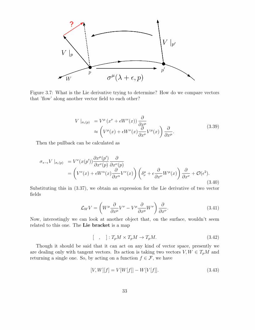
Figure 3.7: What is the Lie derivative trying to determine? How do we compare vectorsthat ’flow’ along another vector field to each other?

V |σε(p) = V µ (xν + εW ν(x))∂

∂xµ

≈(V µ(x) + εW ν(x)

∂

∂xνV µ(x)

)∂

∂xµ.

(3.39)

Then the pullback can be calculated as

σ∗−εV |σε(p) = V ν(x(p′))∂xµ(p′)

∂xν(p)

∂

∂xν(p)

=

(V ν(x) + εWα(x)

∂

∂xαV ν(x)

)(δµν + ε

∂

∂xνW µ(x)

)∂

∂xν+O(ε2).

(3.40)Substituting this in (3.37), we obtain an expression for the Lie derivative of two vectorfields

LWV =

(W µ ∂

∂xµV ν − V µ ∂

∂xµW ν

)∂

∂xν. (3.41)

Now, interestingly we can look at another object that, on the surface, wouldn’t seemrelated to this one. The Lie bracket is a map

[ , ] : TpM × TpM → TpM. (3.42)

Though it should be said that it can act on any kind of vector space, presently weare dealing only with tangent vectors. Its action is taking two vectors V,W ∈ TpM andreturning a single one. So, by acting on a function f ∈ F , we have

[V,W ][f ] = V [W [f ]]−W [V [f ]]. (3.43)

33

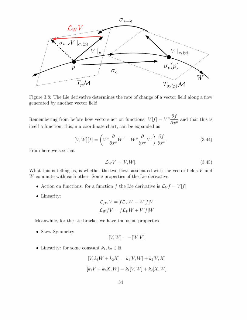
Figure 3.8: The Lie derivative determines the rate of change of a vector field along a flowgenerated by another vector field

Remembering from before how vectors act on functions: V [f ] = V µ ∂f

∂xµand that this is

itself a function, this,in a coordinate chart, can be expanded as

[V,W ][f ] =

(V µ ∂

∂xµW ν −W µ ∂

∂xµV ν

)∂f

∂xν. (3.44)

From here we see that

LWV = [V,W ]. (3.45)

What this is telling us, is whether the two flows associated with the vector fields V andW commute with each other. Some properties of the Lie derivative:

• Action on functions: for a function f the Lie derivative is LV f = V [f ]

• Linearity:LfWV = fLVW −W [f ]V

LWfV = fLVW + V [f ]W

Meanwhile, for the Lie bracket we have the usual properties

• Skew-Symmetry:[V,W ] = −[W,V ]

• Linearity: for some constant k1, k2 ∈ R

[V, k1W + k2X] = k1[V,W ] + k2[V,X]

[k1V + k2X,W ] = k1[V,W ] + k2[X,W ]

34

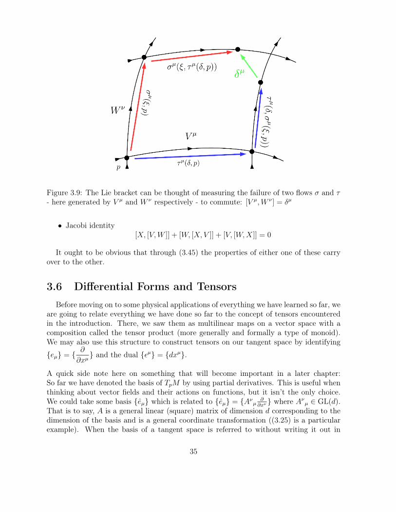
Figure 3.9: The Lie bracket can be thought of measuring the failure of two flows σ and τ- here generated by V µ and W ν respectively - to commute: [V µ,W ν ] = δµ

• Jacobi identity[X, [V,W ]] + [W, [X, V ]] + [V, [W,X]] = 0

It ought to be obvious that through (3.45) the properties of either one of these carryover to the other.

3.6 Differential Forms and TensorsBefore moving on to some physical applications of everything we have learned so far, we

are going to relate everything we have done so far to the concept of tensors encounteredin the introduction. There, we saw them as multilinear maps on a vector space with acomposition called the tensor product (more generally and formally a type of monoid).We may also use this structure to construct tensors on our tangent space by identifying

eµ = ∂

∂xµ and the dual εµ = dxµ.

A quick side note here on something that will become important in a later chapter:So far we have denoted the basis of TpM by using partial derivatives. This is useful whenthinking about vector fields and their actions on functions, but it isn’t the only choice.We could take some basis eµ which is related to eµ = Aνµ ∂

∂xν where Aνµ ∈ GL(d).

That is to say, A is a general linear (square) matrix of dimension d corresponding to thedimension of the basis and is a general coordinate transformation ((3.25) is a particularexample). When the basis of a tangent space is referred to without writing it out in

35

partial derivatives, it is known as a non-coordinate basis.

For now, we will be sticking to our normal tangent space basis. The space of tensorsof valence (q, r) at a point is denoted by T qr,pM . A tensor T ∈ T qr,pM can then be ex-panded as

T = T µ1µ2···µqν1ν2···νr∂

∂xµ1⊗ ∂

∂xµ2⊗ · · · ⊗ ∂

∂xµp⊗ dxν1 ⊗ dxν2 ⊗ · · · ⊗ dxνr (3.46)

Taking f : M → N a diffeomorphism, the pullback naturally extends to (q, 0) tensorsas a map f∗ : T q0,p → T

q0,f(p). While for (0, r) tensors the push forward is f ∗ : T rr,f(p) → T 0

r,p.As an example, we take a (1, 1) tensor and function so that in some coordinate chartf : xµ → yµ, and consider

f∗T = f∗

(T µν

∂

∂xµ⊗ dxν

)= T µνf∗

(∂

∂xµ

)⊗ f∗(dxν) = T µν

∂yα

∂xµ∂xν

∂yβ∂

∂yα⊗ dyβ (3.47)

Now, this leads us into out next topic. We note that the composition ⊗ does not sayanything about the symmetry properties of the resultant tensor. We know that fromphysics that tensors can possess symmetric and/or antisymmetric indices, however thetensor product by itself does not allow for permutations of the tensor factors and hencethe indices. What we look at then is a particularly important type of antisymmetric (0, r)tensor called a differential form. Recall from earlier that we made use of the notationΩ1M for the cotangent space calling into mind the question as to the purpose of 1. Nowwe are going to define a totally antisymmetric (0, r) tensor using the wedge product,or exterior product, which, at the simplest level, is a map

∧ : Ω1M ⊗ Ω1M → Ω2M (3.48)

Where Ω2M is the space of totally antisymmetric two forms. For example

∧ (dxµ ⊗ dxν) = dxµ ∧ dxν =1

2(dxµ ⊗ dxν − dxν ⊗ dxµ) (3.49)

so that it is simply the antisymmetrisation of the tensor product which has the property

dxµ ∧ dxν = −dxν ∧ dxµ (3.50)

from where we see that dxµ ∧ dxµ = 0. More generally we can have a differential form

36

dxµ1 ∧ dxµ2 ∧ · · · ∧ dxµr (3.51)

which is referred to as an r-form and is an element of ΩrM the integer r is called thedegree. Meanwhile the wedge product extends to higher degree forms as

∧ : ΩmM ⊗ ΩnM → Ωm+nM (3.52)

From (3.50) , we note the important property

dxµ1 ∧ dxµ2 ∧ · · · ∧ dxµr = 0 (3.53)

if any index is repeated. A general r-form ω ∈ ΩrM is expressed as

ω =1

r!ωµ1µ2···µrdx

µ1 ∧ dxµ2 ∧ · · · ∧ dxµr (3.54)

Now, something interesting to note: If we have a manifold of dimension m, then thehighest degree r of any form, will be r = m. This is because if we have m basis one-formscorresponding to the number of coordinates, we will not be able to build a form with degreehigher than m without repeating any element (according to (3.53)). More generally, dueto the antisymmetry of the wedge product, the maximum number of elements in ΩrM fora manifold with dimension m is (

m

r

)=

m!

(m− r)!r!(3.55)

Generally, for any forms of arbitrary degree ω ∈ ΩrM and ξ ∈ ΩpM we have

ω ∧ ξ = −ξ ∧ ωω ∧ ω = 0

(3.56)

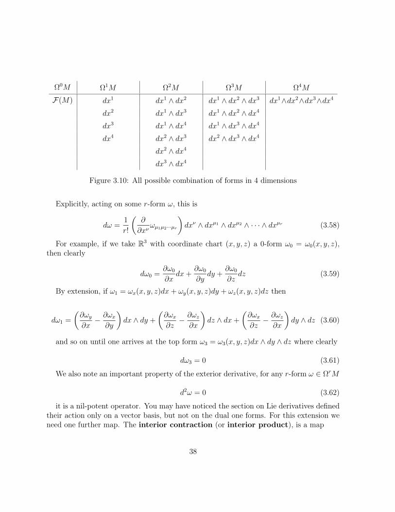
For completeness, we note that Ω0M = F(M), the space of functions. Let’s look atan example: Take a manifold with dim(M) = 4 and a chart with coordinates xµ where1 ≤ µ ≤ 4 and one form basis dxµ. Now what sort of forms can we build out of this?See 3.10.

The highest degree form is called a top-form. Next, we have the exterior derivative,a map

d : ΩrM → Ωr+1M (3.57)

37

Ω0M Ω1M Ω2M Ω3M Ω4M

F(M) dx1 dx1 ∧ dx2 dx1 ∧ dx2 ∧ dx3 dx1∧dx2∧dx3∧dx4

dx2 dx1 ∧ dx3 dx1 ∧ dx2 ∧ dx4

dx3 dx1 ∧ dx4 dx1 ∧ dx3 ∧ dx4

dx4 dx2 ∧ dx3 dx2 ∧ dx3 ∧ dx4

dx2 ∧ dx4

dx3 ∧ dx4

Figure 3.10: All possible combination of forms in 4 dimensions

Explicitly, acting on some r-form ω, this is

dω =1

r!

(∂

∂xνωµ1µ2···µr

)dxν ∧ dxµ1 ∧ dxµ2 ∧ · · · ∧ dxµr (3.58)

For example, if we take R3 with coordinate chart (x, y, z) a 0-form ω0 = ω0(x, y, z),then clearly

dω0 =∂ω0

∂xdx+

∂ω0

∂ydy +

∂ω0

∂zdz (3.59)

By extension, if ω1 = ωx(x, y, z)dx+ ωy(x, y, z)dy + ωz(x, y, z)dz then

dω1 =

(∂ωy∂x− ∂ωx

∂y

)dx ∧ dy +

(∂ωx∂z− ∂ωz

∂x

)dz ∧ dx+

(∂ωx∂z− ∂ωz

∂x

)dy ∧ dz (3.60)

and so on until one arrives at the top form ω3 = ω3(x, y, z)dx ∧ dy ∧ dz where clearly

dω3 = 0 (3.61)

We also note an important property of the exterior derivative, for any r-form ω ∈ ΩrM

d2ω = 0 (3.62)

it is a nil-potent operator. You may have noticed the section on Lie derivatives definedtheir action only on a vector basis, but not on the dual one forms. For this extension weneed one further map. The interior contraction (or interior product), is a map

38

i : TM × ΩrM → Ωr−1M (3.63)

and denotes the contraction of a vector with an r-form. Note that it is not the inverseof the exterior derivative. For V ∈ TM , W ∈ TM , ω ∈ ΩM , η ∈ ΩrM and γ ∈ ΩpM wehave

• iV ω = ω(V ) = (ωµVν)dxµ

(∂

∂xν

)= ωµV

µ

• iV (η ∧ γ) = (iV η) ∧ γ + (−1)deg(γ)η ∧ (iV γ)

• iV iWγ = −iW iV γ

• iV iV γ = 0

Where the second property allows us to extend i to forms of any degree. As an example,let’s look again at R2 and take ω1 = ωxdx + ωydy + ωzdz with a vector V1 = V ∂

∂x. The

we have the contraction

iV1ω1 = iV1(ωxdx) + iV1(ωydy) + iV1(ωzdz) = V ωx (3.64)

Meanwhile, taking ω2 = ωxdx∧dy+ωydy∧dz+ωzdz∧dx we can calculate the contraction

iV1ω2 = iV1(ωxdx ∧ dy) + iV1(ωydy ∧ dz) + iV1(ωzdz ∧ dx)

= V ωxdy − V ωzdz(3.65)

Now we can finally write the Lie derivative for differential forms as

LV ω = diV ω + iV dω (3.66)

An interesting exercise at this point might be to try and derive this expression for oneforms based on the derivation of the Lie derivative for vector fields. Out last point is theaction of the Lie derivative on tensors (since we now know how it acts on the dual basis).Generally, if we take the tensor product of an arbitrary vector and r-form and act withthe Lie derivative we get

LV (W ⊗ ω) = LV (W )⊗ ω +W ⊗ LV (ω) (3.67)

which is simply a version of the usual Leibniz rule for differentiation. So now, if wetake a (1, 1) tensor T ∈ T 1

1 the above means that we have

39

LV T = LV(T µν

∂

∂xµ⊗ dxν

)= V [T µν ]

∂

∂xµ⊗ dxν + T µνLV

(∂

∂xµ

)⊗ dxν + T µν

∂

∂xµ⊗ LV (dxν)

(3.68)

remembering that we also need to act on the scalar component T µν .

40

Chapter 4

Differential Geometry

In Chapter 3 we have studied manifolds in the most abstract way. It is very remarkablehow far we can get by studying those geometrical structures without even defining theconcept of distance. In this chapter we take a step further and we introduce the conceptof metric. This is a fundamental concept in geometry since it enables us to define everysingle geometrical quantity, including distances, angles and volumes, in terms of it. As amatter of fact, one could argue that the metric is the borderline between topology andgeometry, even though this subject is far more subtle than it seems.

The metric also appears everywhere in physics, specially in General Relativity where itplays the role of a fundamental tensor field in nature, interacting with matter accordinglyto the Einstein’s field equation. We will see more on this in the second part of this course.For the time being, let’s see how it beautifully appears in pure geometry.

4.1 MetricWe know from Euclidean geometry that the dot product satisfies the following prop-

erties for u, v ∈ Rn and a, b ∈ R:

1. Symmetry: u · v = v · u

2. Distributivity: u · (av + bw) = au · v + bu · w

3. If u · v = 0 for all v ∈ Rn, then u = 0.

It turns out that these properties are the most important properties that characterizesuch kind of product. In order to generalize this notion of product to smooth manifolds,

41

we have to keep these properties in mind and take them as axioms. Then we get thefollowing definition.

Definition 4. Let V be a real vector space of finite dimension. A real inner product onV is a map V × V → R that assigns a real number 〈u, v〉 ∈ R to every pair of vectorsu, v ∈ V satisfying the following three conditions:

1. Symmetry: 〈u, v〉 = 〈v, u〉

2. Distributivity: 〈u, av + bw〉 = a〈u, v〉+ b〈u,w〉

3. If 〈u, v〉 = 0 for all v ∈ V , then u = 0.

Now we are able to introduce the object that gives name to this section. A metrictensor (or simply metric) on a smooth manifold M is a (0, 2)-tensor field1 satisfying thefollowing axioms:

1. Symmetry: g(X, Y ) = g(Y,X)

2. Positive definiteness: g(X,X) > 0 if X 6= 0.

This means that the metric assigns an inner product structure to every tangent spaceof a manifold M , that is, for every p ∈ M the map gp : TpM × TpM → R is an innerproduct. Sometimes we will also use the notation 〈X, Y 〉p

.= gp(X, Y ) to emphasize this

last fact.See that we are assuming the existence of a new object, the metric is not a consequence

of the previous theory of smooth manifolds. That is the why we say it is an additionalstructure and we call the pair (M, g), formed by a smooth manifold M together with ametric g, by Riemannian manifold.

We may go even further relaxing the positive-definite condition of the metric andinstead assuming that it is just non-degenerate g(X, Y ) 6= 0. A manifold together withsuch a metric is called pseudo-Riemannian manifold or semi-Riemannian manifold.

Example 4.1.1.

1A tensor field on a manifold M is a bit more general than a tensor (not a field) in the followingsense. Let F(M) be the set of all smooth real-valued functions on M . Then a (r, s)-tensor field is definedto be F-linear (instead of R-linear as is the case for tensors) in each of its arguments. For example, a(0, 2)-tensor field T satisfies

Tp(fX + gY ) = f(p)Tp(X) + g(p)Tp(Y ), p ∈M and f, g ∈ F(M).

42

1. The real space Rn together with the dot product is a Riemannian manifold calledEuclidian space and denoted En

2. Spacetime together with the metric given as a solution of Einstein’s equations is apseudo-Riemannian manifold

3. Any surface immersed in En is a Riemannian manifold

4. The configuration space of a Lagrangian mechanical system is a Riemannian mani-fold

In any coordinate system (U ;xi) we can write

g = gijdxi ⊗ dxj, (4.1)

where gij = g(∂i, ∂j) are the coefficients of the metric tensor. In the physics literature gijis what is called metric tensor, but keep in mind that this is an abuse of nomenclature.If we introduce the symmetric product of two 1-forms ω and η, denoted by juxtaposition,the notation used in Equation 4.1 can be shortened:

ωη =1

2(ω ⊗ η + η ⊗ ω).

Due to the symmetry of gij, Equation 4.1 can be written in the following way:

g = gijdxidxj. (4.2)

As it was stressed before, all of the geometrical concepts can be written in terms of themetric. The canonical way of defining distance in Euclidean space, for example, is takingthe square root of the inner product. Since the metric assigns an inner product to eachpoint of a manifold, one would conclude that

‖ · ‖ =√g(·, ·).

Moreover, the length of a curve α on a manifold is defined to be

s =

∫‖α′(t)‖dt =

∫ √g(α′(t), α′(t))dt =

∫ √gijdxi

dt

dxj

dtdt.

43

Then, from the fundamental theorem of calculus, we get the formal expression (in thepoor sense2) usually taken by physicists as the “definition” of the metric

ds2 = gijdxidxj. (4.3)

It is important to note that Equation 4.3 is very formal and objects like dxidxj 3 and ds2

have no mathematical meaning here. But fortunately, the notation used in differentialand integral calculus is very good and physicists do not need to know about differentialforms to proceed with their formal calculations.

Another example is the angle between two tangent vectors X and Y on a manifold isgiven by

cos θ =g(X, Y )

‖X‖‖Y ‖=

g(X, Y )√g(X,X)g(Y, Y )

and as we can see it is written solely in terms of the vectors and of the metric.We will close this section by showing that the metric establishes an isomorphism be-

tween vectors and covectors. Let u = ui∂i be a vector on a manifold M equipped with ametric g. We can define a covector Tu by

Tu(v) =∑i

g ⊗ u(∂i, v, dxi).

Exercise 4.1.1. Convince yourself that Tu is indeed a covector.

Exercise 4.1.2. Show that Tu(v) = g(u, v).

Its coordinates are given by

ui ≡ Tu(∂i) = gijuj. (4.4)

This process is called lowering the index. Conversely, if ω = ωidxi is a covector, then the

vector Tω defined byTω(ρ) =

∑i

g−1 ⊗ ω(dxi, ρ, ∂i),

where g−1 = gij∂i ⊗ ∂j is the inverse of the metric g, has components

ωi = gijωj. (4.5)2When one speaks about formality in mathematics, he means the management of objects concerning

their form and not the mathematical concept behind them. In physics formality means exactly theopposite.

3Observe that this is not the symmetric product defined above. Instead, this is the result of “canceling”dt’s from both sides of the equation.

44

This process is called raising the index. This shows that for every vector there is acorresponding covector and vice versa. Componentwise, they are simply related throughthe metric as in Equations (4.4) and (4.5).

Exercise 4.1.3. Show that raising and lowering index in sucession produces no effect.This is the reason we can keep the same kernel letter u for the vector components ui andthe covector components ui.

4.2 ConnectionsA curve in Euclidean space is straight if and only if its acceleration vanishes identically.

As we know, this is a very important feature of Euclidean geometry and one of the mostfundamental concepts in mechanics as well. Hence, it would be great if we could keepthis idea on general smooth manifolds and then look for the “straight lines” over them. Itturns out it is completely possible to do so if we generalize the notion of acceleration and,in turn, the concept of derivative of vectors. The latter can be easily generalized since wealways expect that any notion of first derivative should satistify the linear and Leibnitzrules. As such, we are going to introduce the covariant derivative as a primitive conceptsatisfying these properties. If T (M) is the set of all smooth vector fields on a manifoldM , then an affine connection (or simply connection) ∇ is a map

∇ : T (M)× T (M)→ T (M) (4.6)(X, Y ) 7→ ∇XY (4.7)

which satisfies the axioms

∇X(Y + Z) = ∇XY +∇XZ, (4.8a)∇(X+Y )Z = ∇XZ +∇YZ, (4.8b)∇(fX)Y = f∇XY, (4.8c)∇X(fY ) = X[f ]Y + f∇XY, (4.8d)

where f : M → R is any differentiable function, X, Y, Z ∈ T (M) and X[f ] represents thedirectional derivative of f in the direction of X at p, defined by

X[f ] =d

dtf(p+ tX)

∣∣∣∣t=0

=∂f(p)

∂xiX i. (4.9)

The last equality of 4.9 was resulted through the application of the chain rule.

45

The connection produces a derivative ∇XY with the above properties, called covariantderivative. Intuitively, the value of ∇XY at a point p ∈ M is the rate of change of Y inthe direction of the unit vector X(p).

The covariant derivative of a vector field Y along a curve γ : R→M is defined to be

DY

dt= DγY,

where γ is the tangent vector to the curve. On a manifold there are infinite many differentways to define a connection that could satisfy Equations (4.8). Despite this, we can restrictthis range of options if we demand that such object obeys some other properties. In thissense, a Levi-Civita connection is a connection such that, for any X, Y, Z ∈ T (M):

∇X [g(Y, Z)] = g(∇XY, Z) + g(Y,∇XZ), (4.10)[X, Y ] = ∇XY −∇YX, (4.11)

where [X, Y ] is the Lie bracket of the vector fields X and Y .The property (4.10), known as compatibility with the metric, says the metric is pre-

served along any curve on M and, hence, angles and volumes are also kept constant. Onthe other hand, the relation (4.11) implies the symmetry of the connection and of theChristoffel symbols, as we will see later on, and is associated to torsionless connections.Unless stated otherwise, we are going to consider only Levi-Civita connections.

In what follows we will illustrate some of the concepts introduced above with concreteexamples. The simplest case is the one of vector fields in the Euclidean space R3. In thiscase the covariant derivative

∇ : T (E3)× T (E3)→ T (E3)

of W = W i∂i with respect to the vector X at p is defined by

∇XW = =d

dtW (p+ tX)(0), (4.12)

=d

dtW i(p+ tX)(0)∂i, (4.13)

= X[W i]∂i, (4.14)

i.e., the covariant derivative is the directional derivative of the vector field W in thedirection of v, which is the derivative of the Equation (4.9) calculated for each componentof W . To show that (4.13) is in fact a covariant derivative, we just need to verify it

46

satisfies the properties (4.8). To do this we just have to verify them for each componentof the Equation (4.14). Therefore, from the linearity of the usual derivative, we get (4.8a):

∇X(Y i + Zi) = X[Y i + Zi] =d

dt(Y i + Zi)(p+ tX)

∣∣∣∣t=0

=d

dt

[Y i(p+ tX) + Zi(p+ tX)

] ∣∣∣∣t=0

= X[Y i] +X[Zi] = ∇XYi +∇XZ

i.

Using the chain rule we get (4.8b):

∇X+YZi =

d

dtZi(p+ t(X + Y ))

∣∣∣∣t=0

=∂Zi

∂xj(Xj + Y j)

=∂Zi

∂xjXj +

∂Zi

∂xjY j

= X[Zi] + Y [Zi] = ∇XZi +∇YZ

i.

The relation (4.8c) is obtained through the direct application of the chain rule and of theLeibnitz rule:

∇fXYi = (fX)[Y i] =

d

dtY i(p+ tfX)

∣∣∣∣t=0

=∂Y i

∂xjd

dt(pj + tfXj)

∣∣∣∣t=0

=∂Y i

∂xj

[f + t

(∂f

∂xkxk)] ∣∣∣∣

t=0

Xj

=∂Y i

∂xjfXj

= fX[Y i] = f∇XYi.

Lastly, property (4.8d) is resulted from the application of the Leibnitz rule:

∇XfYi = X[fY i] =

d

dt(fY i)(p+ tX)

∣∣∣∣t=0

=d

dtf(p+ tX)

∣∣∣∣t=0

Y i + fd

dtY i(p+ tX)

∣∣∣∣t=0

= X[f ]Y i + fX[Y i] = X[f ]Y i + f∇XY.

47

Exercise 4.2.1. The covariant derivative of vector fields on a surface S immersed in R3

is defined by the projection of (4.13) on the surface S:

∇ : T (S)× T (S)→ T (S) (4.15)

(X, Y ) 7→ ∇XY = ∇XY − 〈∇XY,N〉N, (4.16)

whereN =

∂u × ∂v‖∂u × ∂v‖

is the normal vector field to the surface, also known as Gauss map, and ∇XY representsthe Euclidean covariant derivative given by Equation (4.14). Prove that Equation (4.16)is indeed a covariant derivative.

Geometrically, the definition (4.16) measures the rate of variation of a vector field Y ,defined over a surface S, in the direction of the unit vector X, also defined over S. Ifwe imagine γ(t) as being the curve which describes the position of a particle constrainton a surface S, then the covariant derivative ∇γ′(t)γ

′(t) has the meaning of the particle’sacceleration vector over this surface.

It is interesting to note that so far the covariant derivative has been used abstractly,that is, without the need of introducing a reference frame. However, it is useful to expressit as coordinates of such a reference system to make calculations easier. So let ∂i(p)be a basis for TpM . The covariant derivative of a vector from this basis with respect toanother vector from the same basis is again another vector of this basis. Therefore, wecan write

∇∂i∂j = Γkij∂k, (4.17)

where the coefficients Γkij are called Christoffel symbols. Moreover, from Equation (4.11)we find that:

[∂i, ∂j] = ∇∂i∂j −∇∂j∂i

= (Γkij − Γkji)∂k.

Since ∂i∂jf = ∂j∂if , it follows that:

Γkij = Γkji, (4.18)

i.e., the Christoffel symbols are symmetric in the lower indices.

48

Hence, in order to specify the covariant derivative of arbitrary vector fields is enough tospecify it for each basis vector ∂j with respect to ∂i. Then, using Equation (4.17) togetherwith the properties (4.8), we find that for generic vectors X = X i∂i and Y = Y j∂j that:

∇XY = ∇Xi∂i(Yj∂j) (4.19)

= X i∇(Y j∂j) (4.20)= X iY j∇∂i∂j +X i∂j∇∂iY

j (4.21)

= X iY jΓkij∂k +X i∂Yj

∂xi∂j. (4.22)

Since the index j in the last term is dummy, we can change it for k and we get

∇XY =

(∂Y k

∂xi+ Y jΓkij

)X i∂k. (4.23)

If we repeat the above argument for vector fields Y defined along curves γ, we wouldget

DY

dt=

(dY k

dt+ Y jΓkij

dxi

dt

)∂k. (4.24)

Exercise 4.2.2. Prove Equation (4.24).

It is possible to find the Christoffel coefficients Γkij only in terms of the metric and itsderivatives from the metric compatibility condition (see Equation (4.10)):

0 =∂gik∂xl− gmkΓmkl − gimΓmkl. (4.25)

Using that the Christoffel symbols are symmetric in the lower indices, Equation (4.25)can be solved explicitly for Γkij:

Γkij =gkl

2

(∂gjl∂xi

+∂gli∂xj− ∂gij∂xl

). (4.26)

Be aware that the Equation (4.26) only holds for the Levi-Civita connection. If torsionis included, as happens in Einstein-Cartan gravity for example, the Christoffel symbolscannot be expressed in terms of the metric and its derivatives. In fact, connections are,in general, completely independent of the metric since they form different mathematicalstructures. Fortunately, General Relativity has the Levi-Civita connection and Equation(4.26) is all we need to specify it.

49

4.3 GeodesicsA vector field Y is said to be parallel along a curve γ if its covariant derivative along

γ vanishes for all t in the curve’s parameter range, that is,

DY

dt= 0, t ∈ I ⊂ R. (4.27)

A curve whose tangent vector is parallel along itself is called a geodesic:

∇γ γ = 0, t ∈ I. (4.28)

Therefore, the geodesics are precisely the “straight lines” on manifolds that we were lookingfor, simply because their accelerations vanish.

According to Equation (4.24), in a coordinate system (U ;xi) Equation (5.1) becomes

d2xk

dt2+ Γkij

dxj

dt

dxi

dt= 0. (4.29)

This is the equation which describes the geodesics in a neighborhood U of a manifold.It must be observed that Equation (4.29) was determined without specifying any specificconnection, hence wether Christoffel symbols in this equation can be determined throughthe metric, as in Equation (4.26), or not depends upon the chosen connection.

The parameter t used to parametrize γ such that it satisfies Equation (4.29) is calledaffine parameter. Under a reparametrization of γ, say t′ = f(t), the tangent vectorbecomes

γ′ =dxi

dt′∂i =

1

f ′(t)

dxi

dt∂i,

where f ′(t) = df/dt and, using Equation (4.29), we have

d2xk

dt′2+ Γkij

dxj

dt′dxi

dt′=

1

f ′(t)

d

dt

(1

f ′(t)

)dxi

dt

= − f′′(t)

f ′(t)2dxi

dt′.

Hence the new parameter t′ is an affine parameter if, and only if, f ′′(t) = 0 or t′ = at+ bfor a, b real constants. This shows that the fact of being a geodesic depends on theparametrization. Curves that can be transformed into geodesics through a reparametriza-tion are called pre-geodesics.

50

4.4 Torsion and CurvatureIn the transformation law of Γijk, the term involving second derivatives is symmetric in

the indices jk. It follows that the antisymmetrized quantity

T ijk = Γijk − Γikj (4.30)

does transform as a tensor, due to the cancellation of the non-tensorial parts. To expressthis idea in a non-coordinate way, we define the torsion map τ : T (M)×T (M)→ T (M)by

τ(X, Y ) = ∇XY −∇YX − [X, Y ].

Exercise 4.4.1. Show that τ is antisymmetric, i.e., τ(X, Y ) = −τ(Y,X) and F -linear(see the footnote in the beginning of this chapter).

Hence τ gives rise to a tensor field T of type (1, 2) defined as

T (ω,X, Y ) = 〈ω, τ(X, Y )〉.

It is called torsion tensor of the connection ∇.

Exercise 4.4.2. By applying T to basis vectors, prove that its coefficients in a localcoordinate chart (U ;xi) is given by Equation (4.30).

We call a connection torsion-free or symmetric if its torsion tensor vanishes identically,T = 0. In this case, Equation (4.30) shows that its components are symmetric withrespect to any coordinates.

A similar problem occurs when commuting repeated covariant derivatives on a vectoror tensor field. The map P : T ∗(M)× T (M)× T (M)× T (M)→ F(M) defined by

P (ω,X, Y, Z) = 〈ω,∇X∇YZ,∇Y∇XZ〉

fails to be a tensor of type (1, 3) since it is not F -linear in the three vector field arguments.To remedy this we proceed in the same way as before for creating the torsion tensor.

For any vector fields X, Y define the operator ρX,Y : T (M)→ T (M) by

ρX,YZ = ∇X∇YZ −∇Y∇XZ −∇[X,Y ]Z.

Exercise 4.4.3. Prove that ρX,YZ is F -linear in all of its components.

51

Therefore, we can define a tensor field of type (1, 3) by setting

R(ω,X, Y, Z) = 〈ω, ρX,YZ〉,

known as Riemann curvature tensor of the connection ∇.In a local coordinate chart (U ;xi), the components of the curvature tensor is given by

Rijkl = R(dxi, ∂j, ∂k, ∂l)

= 〈dxi,∇k∇l∂j −∇l∇k∂j −∇[∂k,∂l]∂j〉= 〈dxi,∇k(Γ

mjl∂m)−∇l(Γ

mjk∂m)〉

= 〈dxi,Γmjl,k∂m + ΓmjlΓpmk∂p − Γmjk,l∂m − ΓmjkΓ

pml∂p〉,

where Γmjl,k =∂Γmjl∂xk

. Therefore

Rijkl = Γijl,k + ΓmjlΓ

imk − Γijk,l − ΓmjkΓ

iml. (4.31)

The Ricci (curvature) tensor is then defined by

Ric(X,Z) =∑i

R(dxi, X, ∂i, Z),

whose coordinates areRij ≡ Ric(∂i, ∂j) = Rk

ikj = glkRlikj. (4.32)

This process in which two indices are set equal to each other and summed over is calledcontraction. Contracting again we get the Ricci scalar

R = Rii = gijRij. (4.33)

If we are using the Levi-Civita connection, then the Riemann tensor, the Ricci tensor andthe Ricci scalar can be calculated directly from the metric. That is why the metric ischosen to be the fundamental field in General Relativity; it carries all of the geometricaland physical information we need.

52

Part II

Applications

53

Chapter 5

General Relativity

Now we have seen the basics of differential geometry, it is about time we moved onto some applications. One may wonder as to the purpose of the previous sections (inparticular why they seem so long). The answer to this, is that we are trying to obtainnew intuition for something we are already quite familiar with. For this reason, it isimportant to spend some time familiarizing oneself with the basics, in this case the notionsof topological spaces, manifolds etc. The actual application should then be almost only adetail. What we are trying to do, is not to learn new physics, but rather to think aboutthe physics we already know in a different way. The following sections are not intendedas - could never be - a re-derivation of all of physics based on differential geometry, butrather a list of specific examples. Hopefully familiar ones, they are intended to show howwe can take the contents of the previous section and apply to things we already know andhopefully, gain some insight by doing so. At the end of the day, a formalism (like tensorcalculus or path integrals) is only a tool and it is important to have the knowledge tochoose the right tool for the job. In this section we will be looking specifically at GeneralRelativity (GR). What follows assumes that the reader is already familiar with GR at thelevel of an undergraduate course. We are going to look some (hopefully) familiar examplesand then cast them in different ways based on the previous chapters.

5.1 PostulatesThe theory of GR is just a match of geometrical concepts with physical ones. Pre-

cisely, this is done by setting up the postulates of GR as follows. The universe is afour-dimensional Pseudo-Riemannian manifold (M, g) of index +2 (i.e., with a metricwhose signature has 3 plus signs corresponding to spatial coordinates and 1 minus sign

54

corresponding to time coordinate; the index is defined to be the sum of these signs) calledspacetime. Its points are called events. Test particles “free fall” along spacetime, sincethey are subjected to no external forces, following its geodesics:

d2xµ

ds2+ Γµνρ

dxν

ds

dxρ

ds= 0. (5.1)

The geodesics followed by massive particles are assumed to be time-like, whereas masslessparticles, e.g. photons, move along null-like geodesics. Since the geodesic equation (5.1)does not depend on the mass of the particle, all particles have the same geodesic. Thisis the equivalence principle: all particles undergo the same acceleration in a gravitationalfield.

The Einstein field equations are

Ric− 1

2Rg = 8πT, (5.2)

or in a coordinate chartRµν −

1

2Rgµν = 8πTµν ,

where T = Tµνdxµ ⊗ dxν is the stress-energy tensor of the matter fields and we are

using units such that Newton constant and the speed of light are G = c = 1. Keep inmind that Equation (5.2) cannot be proved, it was first obtained by brute force (justlike Newton’s second law and Schrödinger equation) in an attempt of getting a relationbetween curvature and energy. That being said, we can adopt a variational approachin which the field equations (5.2) can be deduced. This is accomplished by using theHilbert-Einstein action

S =

∫ √− det(g)R. (5.3)

Varying this action with respect to the metric field and setting the result to zero leadsus to (5.2). However, by adopting the above action we are just shifting our ignorancebecause now what cannot be proved is Equation (5.3).

5.2 Tetrad formalismTo begin with, we are going to take a closer look at something that was already touched

on in previous sections, a non-coordinate basis (also called a tetrad). In the sectionon manifolds, we formulated all out quantities in terms of the tangent space basis ∂µ.It has the drawback of explicitly depending on some choice coordinates xµ and as you

55

may recall, no one coordinate systems is unique and there is generally no canonical choice(that is, there is no preferred system of coordinates). An example of where this becomesan issue, is the Schwarzschild spacetime which, if you recall, describes black holes. Sinceit is by definition spherically symmetric, the easiest choice of coordinate chart is sphericalcoordinates. But, as you hopefully recall, this leaves us with an apparent singularity atthe black holes event horizon which can be dealt with by a change in coordinates (e.g.Eddington-Finkelstein or Kruskal-Szekeres). What we see however, is a coordinate sys-tem which makes calculations easy but suffers from a significant pathology while tryingto eliminate it, can make the analysis all the more difficult. Mathematically speaking,neither of these scenarios is preferred and both are equally valid in the regions their cov-erings overlap. However, we still need some notion of coordinates if we are to do physics.

We are going to avail ourselves of a tetrad basis eµ which is related to our tangentspace basis by some coordinate transformation

eα =∂yν

∂xα∂

∂yν(5.4)

I you recall, any coordinate bases can be related to any other by a transformation ofthis kind. Now however, we are going to denote the transformation matrix by

eνα =∂yν

∂xα(5.5)

and take a look at some of its properties. Firstly, and most obviously, we can recast(5.4) as

eα = eνα∂

∂xν(5.6)

While, conversely for the dual basis dxµ on T ∗M , we have

eα = eανdxν (5.7)

We then require that the basis eα be orthonormal, that is, the inner productsatisfies

〈eα, eβ〉 = δαβ (5.8)

This means we have a metric in this basis given by

g = gµνdxµ ⊗ dxν = gµνeα

νeβνeα ⊗ eβ = ηµνe

α ⊗ eβ = η (5.9)

56

where η is the flat space Minkowski metric

η =

−1 0 0 0

0 1 0 0

0 0 1 0

0 0 0 1

(5.10)

This is nothing more than a coordinate transformation into a frame where the metricis flat. The matrices eαν are called vierbein 1 and correspond to whichever coordinatetransformation maps one to this frame. But hold on, what about curvature, surely youcan’t just do a coordinate transformation and get rid of it? Indeed one can’t. Usually,our tangent space basis ∂µ is rather trivial, so that one has, for example, [∂µ, ∂ν ]f = 0for any function f . This is obvious since partial derivatives commute with each other.However, the basis eα isn’t as trivial, since it will generally contain some functionaldependence and then [eµ, eν ]f 6= 0 as for the general Lie bracket of vector fields. Whatthis special coordinate transformation amounts to is taking all the parametric dependenceout of the metric and putting it into the basis vectors in such a way that they are or-thonormal. The most astounding thing about this, is that it is always possible to findsuch a transformation. Also, it is worth noting that a basis given by (5.4) will have a Liebracket of the form

[eµ, eν ] |p= cµνα(p)eα |p (5.11)

Further, we note that eαµeνα = δµν and eαµeµβ = δαβ. It is important to distinguish

between the indices on this matrix when raising and lowering, since this is done in dif-ferent frames with different metrics. For example, the transformation in (5.5) one haseµα = gµνe

να and eνβ = ηαβeνα. Also note eναeνβ = ηαβ and eναeµα = gµν .

Let’s have look at some examples. First consider the standard spherical metric on S2

ds2 = dθ ⊗ dθ + sin2(θ)dφ⊗ dφ (5.12)

This can easily be converted into the form (5.9) if we take a basis

e1 = dθ e2 = sin(θ)dφ (5.13)

1Vierbein is German and translates as ’four-leg’ which is specific to four dimensions. In arbitrarydimensions the term vielbein is used (many-leg). In a specific number of dimensions one can also have,for example zweibein, dreibein etc. (receptively two-leg and three-leg)

57

The tetrad is then read of as

eαµ =

(1 0

0 sin(θ)

)(5.14)

Now, consider the Schwarzschild metric in spherical coordinates:

ds2 = −(

1− 2GM

r

)dt⊗dt+

(1− 2GM

r

)−1dr⊗dr+r2dθ⊗dθ+r2 sin2(θ)dφ⊗dφ (5.15)

Here we see similarly

e0 =

(1− 2GM

r

)1/2

dt e1 =

(1− 2GM

r

)−1/2dr

e2 = rdθ e3 = r sin(θ)dφ

(5.16)

with

eαµ =

(1− 2GM

r

)1/2

0 0 0

0

(1− 2GM

r

)−1/20 0

0 0 r 0

0 0 0 r sin(θ)

(5.17)

A more interesting example is perhaps a non-diagonal metric (in two dimensions forsimplicity)

ds2 = du⊗ dv + dv ⊗ du (5.18)

Here we can take

e1 =1√2

(du− dv) e2 =1√2

(du+ dv) (5.19)

which you can verify:

ds2 = −e1 ⊗ e1 + e2 ⊗ e2 (5.20)

Does it look familiar? This corresponds to

58

eαµ =1√2

(1 1

1 −1

)(5.21)

What all of this hopefully makes clear is that we can always choose to work in a non-coordinate basis. We also note that this basis can be composed the same way as thecoordinate basis using the wedge product i.e. eµ∧eν . The top form in this basis is specialand referred to as a volume form

ΩM = e1 ∧ e2 ∧ · · · ∧ em =√| g |dx1 ∧ dx2 ∧ · · · ∧ dxm (5.22)

where g is the determinant of the metric. This is nothing more than the volume elementfrom GR (think of integral measures

∫ √| g |dmx). Lastly, we mention for convenience

sake, a coordinate free version of raising and lowering indices. The metric can be viewedas an isomorphism g : TpM → T ∗pM and g : T ∗pM → TpM . Explicitly, for a vectorV ∈ TpM we will denote its metric dual one-form as V ∈ T ∗pM where these are relatedby by

V = g(V,−) = g(V αeα, eβ)eβ = ηαβVαeβ = Vβe

β (5.23)

For a one form ω ∈ T ∗pM its corresponding metric dual is

ω = g−1(ω,−) = g−1(ωαeα, eβ)eβ = ηαβωαeβ = ωβeβ (5.24)

It should be evident that we have ˜ω = ω and ˜V = V . A note on conventions, inthe literature you might find this method a raising and lowering indices referred to as amusical isomorphism. So, lowering the index of a vector is, independently of any basis,denoted by V [ and likewise raising the index of a one form by ω]. If you are familiar withmusical notation, you might see the logic behind this, although we will not be using thisparticular notation here.

5.3 Hodge MapI we are to examine an alternative formulation of GR, we are going to need one more,

rather useful map. Let’s take another look at the Table 5.1, but now repeat the sameexercise in a non coordinate basis of dimension four.

59

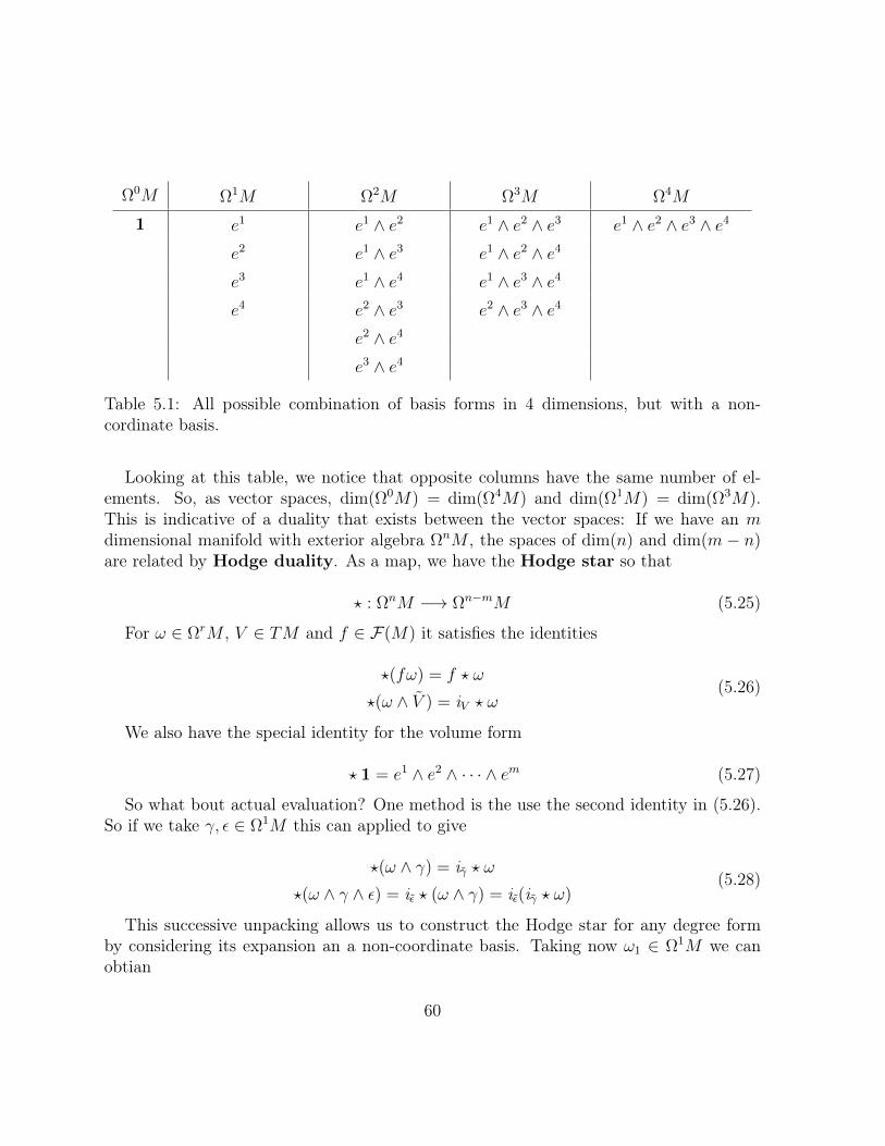
Ω0M Ω1M Ω2M Ω3M Ω4M

1 e1 e1 ∧ e2 e1 ∧ e2 ∧ e3 e1 ∧ e2 ∧ e3 ∧ e4

e2 e1 ∧ e3 e1 ∧ e2 ∧ e4

e3 e1 ∧ e4 e1 ∧ e3 ∧ e4

e4 e2 ∧ e3 e2 ∧ e3 ∧ e4

e2 ∧ e4

e3 ∧ e4

Table 5.1: All possible combination of basis forms in 4 dimensions, but with a non-cordinate basis.

Looking at this table, we notice that opposite columns have the same number of el-ements. So, as vector spaces, dim(Ω0M) = dim(Ω4M) and dim(Ω1M) = dim(Ω3M).This is indicative of a duality that exists between the vector spaces: If we have an mdimensional manifold with exterior algebra ΩnM , the spaces of dim(n) and dim(m − n)are related by Hodge duality. As a map, we have the Hodge star so that

? : ΩnM −→ Ωn−mM (5.25)

For ω ∈ ΩrM , V ∈ TM and f ∈ F(M) it satisfies the identities

?(fω) = f ? ω

?(ω ∧ V ) = iV ? ω(5.26)

We also have the special identity for the volume form

? 1 = e1 ∧ e2 ∧ · · · ∧ em (5.27)

So what bout actual evaluation? One method is the use the second identity in (5.26).So if we take γ, ε ∈ Ω1M this can applied to give

?(ω ∧ γ) = iγ ? ω

?(ω ∧ γ ∧ ε) = iε ? (ω ∧ γ) = iε(iγ ? ω)(5.28)

This successive unpacking allows us to construct the Hodge star for any degree formby considering its expansion an a non-coordinate basis. Taking now ω1 ∈ Ω1M we canobtian

60

? ω1 = ?(ω1µeµ) = ieµ ? ω1µ = ieµω1µ ? 1 (5.29)

Where the Hodge star of a scalar quantity is simply that scalar multiplied by thevolume form and eµ = eµ. To check this, remember that the action of ? is to map anr-form into an (m− r)-form. Here, we are starting with a one-form and applying ? meansthat we contract the metric dual with the volume form to give an (m− 1)-form. So if wewere in four dimensions, the above would be a three form (see 5.1). Now for ω2 ∈ Ω2M ,we can similarly calculate

? ω2 = ?(ω2µνeµ ∧ eν) = ieµ(?ω2µνe

ν) = ieµ(ieν (ω2µν ? 1)) (5.30)

Generally for ω ∈ ΩrM we can iterate this to give

? ω = ?(ωµ1···µreµ1 ∧ · · · ∧ eµr) = ωµ1···µr(ieµ1 · · · ieµr ? 1) (5.31)

Applying the Hodge star twice returns the original form up to some sign dependent onthe conventions chosen so that

? ?ω = (−1)r(m−r)ω (5.32)

if the metric is Riemannian and

? ?ω = (−1)1+r(m−r)ω (5.33)

if it is Lorentzian. Lastly, we note that we also have an inverse ?−1. By demanding??−1 = ?−1? = id, we get that

?−1ω = (−1)r(m−r) ? ω

?−1ω = (−1)1+r(m−r) ? ω(5.34)

if the metric is Riemannain or Lorentzian respectively. We can use these operationsfor an alternative definition of the inner product between two forms

〈ω, γ〉 = gαβωαγβ = ?−1(ω ∧ ?γ) (5.35)

There is a rather interesting example of this specific to three dimensions. Let’s takeR3 with the basis dx, dy, dz (obviously, in this case eµ = dxµ). The volume form is?1 = dx ∧ dy ∧ dz while for the metric we have

ds2 = dx⊗ dx+ dy ⊗ dy + dz ⊗ dz (5.36)

61

Now consider

?(dx ∧ dy) = i∂y i∂x ? 1

= i∂y i∂x(dx ∧ dy ∧ dz)

= i∂y(dy ∧ dz)

= dz

(5.37)

We are in three dimensions applying the Hodge star to a two form, so the result shouldbe a one form. Repeating, we also get

?(dx ∧ dz) = −dy, ?(dy ∧ dz) = dx (5.38)

This ought to look familiar:

ex × ey = ez, ex × ez = −ey ey × ez = ex (5.39)

What we have just obtained is, in a sense, a generalization of the cross product, butone that can be used in an arbitrary number of dimensions. The cross product in R3 isspecial since it is only in this number of dimensions that we can take the product of twovectors (co-vectors) and obtain another vector. In four dimensions, repeating the abovewould give a two form, in five dimensions a three form and so on. For completeness wealso show

? ? (dx ∧ dy) = ?dz

= i∂z ? (dx ∧ dy ∧ dz)

= dx ∧ dy(5.40)

which gives the same as applying (5.32) directly.

Lastly, we note that there exists a definition of some familiar operators in this formalismthat allows us to apply them in any number of dimensions. For some function f ∈ F(M)and vector V ∈ TpM

grad(f) = df

div(V ) = ?dV

curl(V ) = ?−1d ? V

(5.41)

As an exercise, try to relate these to the usual divergence, gradient and curl operatorsin three dimensions:

62

grad(f) = ∇fdiv(V ) = ∇ · Vcurl(V ) = ∇× V

(5.42)

5.4 Curvature and TorsionWe were introduced to the ideas of connections, curvature and torsion in a previous

chapter. In light of everything we have just covered in this chapter, one may well ask howit all applies to those ideas. To how this changes let’s first consider a connection ∇ andits action on a non-coordinate basis eµ (and its corresponding dual)

∇eνeµ = Γγνµeγ = ωγµ(eν)eγ, (5.43)

where we have introduced a set of m2 one forms ωγµ called connection one-formsrelated to the Christoffel symbols by either Γγνµeγ = ωγµ(eν)eγ = ieν (ω

γµ)eγ or Γγνµe

ν =ωγµ. We can define the curvature two-form

Rαβ =

1

2Rα

βγδeγ ∧ eδ (5.44)

using the Riemann curvature tensor and the torsion two form

Tα =1

2Tαγδe

γ ∧ eδ (5.45)

from the torsion tensor. These satisfy Cartan’s structure equations

deα + ωαβ ∧ eβ = Tα

dωαβ + ωαγ ∧ ωγβ = Rαβ

(5.46)

Further, if our connection is Levi-Civita (that is torsion free and ∇g = 0), we can findthe connection one-forms from our basis using

ωµν =1

2(ieνdeµ − ieµdeν + eαieµieνde

α) (5.47)

Once again, let’s take an example: We look at S2 with the metric

ds2 = dθ ⊗ dθ + sin2(θ)dφ⊗ dφ. (5.48)

We already demonstrated in a previous example that the basis is given by

63

e1 = dθ e2 = sin(θ)dφ (5.49)

with the dual basis

e1 = ∂θ e2 =1

sin(θ)∂φ. (5.50)

So now we can calculate the nonzero connection one-forms as

ω12 = −ω21 = − cot(θ)e2 = cos(θ)dφ. (5.51)

Since we are working with the Levi-Civita connection to obtain this expression, we knowthat the right hand side of the first of Cartan’s structure equations must be zero. Substi-tuting the above confirms the same for the left hand side:

de1 + ω12 ∧ e2 = 0,

de2 + ω21 ∧ e1 = cot(θ)e1 ∧ e2 + cot(θ)e2 ∧ e1 = 0.

(5.52)

Meanwhile, the second structure equation can be solved for the curvature two form togive

R12 = −R21 = −e1 ∧ e2 (5.53)

There are two things to note about this result. Firstly, it is frame independent. Sincethe basis eµ can be identified with the polar basis in any way (so the great circle sectionconnecting the poles can be chosen to lie anywhere) the above answer is valid in all frames.Secondly, if you have ever gone through the rigmarole of calculating the curvature byusing the Christoffel symbols, it is hopefully clear that this way is considerably shorter(Christoffel symbols have 1

2(m2 + m) components while the connection one-forms have

12(m2 −m)). This is a point we are going to illustrate further in the next section.

5.5 Electromagnetism and Einstein’s EquationsAn extremely useful application lies in electromagnetism. Expressed in conventional

vector calculus, Maxwells equations (in differential form) are

64

∇ · E = ρ,

∇ ·B = 0,

∇× E = −∂B∂t,

∇×B = J +∂E

∂t,

(5.54)

where E and B are the electric and magnetic fields respectively, ρ is the charge densityand J the current density. These are related to the vector potential A by

E =∂A

∂t,

B = ∇×A.(5.55)

As you might recall, the operators used here are not suited to general relativity owing tothem being defined only in three dimensions. Using the contents of this section however,we are in a position to recast these in a general and coordinate independent form. Now,we treat A as a one-form. The Maxwell two-form is obtained by

F = dA. (5.56)

Maxwell’s equations are now cast in a much more compact form 2

dF = 0,

d ? F = j,(5.57)

where j is the current three form. As an exercise, take this R1,3 (flat Minkowski space)and by expanding the Maxwell two-form as

F =1

2Fµνdx

µ∧dxν = Exdx∧dt+Eydy∧dt+Ezdz∧dt+Bzdx∧dy−Bydx∧dz+Bxdy∧dz(5.58)

and the current three form

? j = ρdt+ jxdx+ jydy + jzdz (5.59)

try to obtain the Maxwell equation in (5.55). We now turn to Einstein’s equations, howare they to be recast in this form? Take first the contraction

2It has been said that the progress of physics can be tracked through the ever increasing compactifi-cation of Maxwell’s equations.

65

Pµ = Rαµ(ealpha) = iealphaR

αµ (5.60)

called the Ricci one-form. This is related to the Ricci tensor by

Ric = Pµ ⊗ eµ. (5.61)

We then further consider the Einstein three-form

Gµ = Rαβ ∧ ?(eα ∧ eβ ∧ eµ), (5.62)

which we relate back to the traditional Einstein tensor by

Ein = −1

2? Gµ ⊗ eµ. (5.63)

If we then define the curvature scalar by

P = ieαieβRαβ, (5.64)

we can recast this in the more familiar form (try as an exercise)

Ein = Ric− 1

2Pg. (5.65)

We are, however, not obliged to work in this frame and can in fact write Einstein’sequations as

Gµ = 8πτµ, (5.66)

where τµ is the stress-energy-momentum three-form (SEM three-form). A commonexample, drawing on what we covered above, is the SEM three-form for the electromag-netic field

τEMµ =1

2(ieµF ∧ ?F − F ∧ ieµ ? F ) . (5.67)

Or, for a scalar field satisfying the Klein-Gordon equation

d ? dφ−m2φ ? 1 = 0, (5.68)

it is

τSµ =1

2(ieµdφ ∧ ?dφ− dφ ∧ ieµ ? dφ)− 1

2m2φ2 ? eµ. (5.69)

66

Chapter 6

Topological defects on condensedmatter

Differently from particle physics, which tries to understand the matter looking for itsfundamental constituent, condensed matter physics tries to explain it through the emer-gent behavior resulted from the interaction of zillions of electrons, atoms and molecules.To accomplish this, it is necessary to look for the variables and degrees of freedom mostimportant. These variables are often brought together in the so called order parameter,which is a (scalar, vector or tensor) field ψ : X →M that maps points from the physicalspace X into the abstract space M , known as order parameter space. The space M isdefined as the space in which the parameter ψ is varied without changing the energy ofthe system. It is for this reason that this space is also called degeneracy space, since allof the points in this space have the same energy.

Let’s see some examples to better illustrate this idea. The order parameter of a bidi-mensional ferromagnetic material, for instance, is given by the vector field possessingconstant magnitude that describes the spins direction in the material. The degeneracyspace is then a circle whose points correspond to a direction of the vector field. If u andv are orthonormal vectors on the plane, the order parameter can be given by

f(~r) = u cosφ(~r) + v sinφ(~r).

The same order parameter space describes the superfluid helium-4, in which the orderparameter is the complex scalar field with constant magnitude ψ0 but with arbitraryphase φ(~r)

ψ(~r) = ψ0 exp (iφ(~r)).

In this case the degeneracy space can be thought as a unit circle in the complex plane.Another interesting example is the nematic liquid crystal. It is one of the phases of a

67

liquid crystal whose molecules have directional symmetry. This means the molecules arealigned to a vector field N, called director. Considering bidimensional nematics, the orderparameter is the director vector N itself, which takes values on the space S1. However,the director vector also has inversion symmetry; this means that N and −N represent thesame physical state. Therefore, the topological space which describes the nematics phasestates is the projective line RP 1, that is, the space obtained by identifying the pointsp ∈ S1 with their respect antipodes (Figure 6.1).

Figure 6.1: Representation of the manifold RP 1 such that the points P and P ′ areidentified. Figure taken from http://ieeexplore.ieee.org/ieee_pilot/articles/06/ttg2009061457/article.html.

When the space M is degenerated, i.e., formed by only one point, we say ψ (andtherefore the material itself) is homogeneous. Nonetheless, the field ψ(r) in general variespoint to point and there are even regions in the material where ψ is not defined at all.These singular regions are the defects. If this defect can be removed by a continuoustransformation of the order parameter ψ, such that the field configuration be transformedinto a configuration locally homogeneous, we say the defect is topologically unstable. Onthe other hand, if the defect cannot be eliminated by continuous transformations on theorder parameter, we say the defect is topologically stable, or simply that it is a topologicaldefect. The topological defects can be points (no dimension), lines (1 dimension) orsurfaces (2 dimensions). From now on, whenever we say defect is to be understoodtopological defect, unless we explicitly state otherwise.

Let’s suppose that the topological space X is filled with a condensed matter systemto be studied. Suppose also that exists a topological defect in this media. By simplicity,let’s say that this defect is a point defect. Draw a loop α around the defect in X (Figure6.2). Through the order parameter ψ, the loop α is mapped into a loop β = ψ α inM . It is from the loops in M , more precisely from the fundamental group of M , thatwe investigate the topology of M and, consequently, classify the topological defects inX. If M has holes or offer restrictions on the deformation of an arbitrary loop β, X has

68

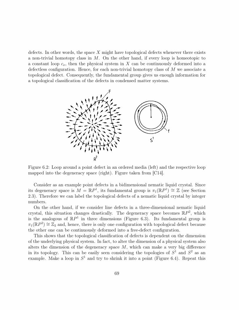
defects. In other words, the space X might have topological defects whenever there existsa non-trivial homotopy class in M . On the other hand, if every loop is homeotopic toa constant loop cx, then the physical system in X can be continuously deformed into adefectless configuration. Hence, for each non-trivial homotopy class of M we associate atopological defect. Consequently, the fundamental group gives us enough information fora topological classification of the defects in condensed matter systems.

Figure 6.2: Loop around a point defect in an ordered media (left) and the respective loopmapped into the degeneracy space (right). Figure taken from [C14].

Consider as an example point defects in a bidimensional nematic liquid crystal. Sinceits degeneracy space is M = RP 1, its fundamental group is π1(RP 1) ∼= Z (see Section2.3). Therefore we can label the topological defects of a nematic liquid crystal by integernumbers.

On the other hand, if we consider line defects in a three-dimensional nematic liquidcrystal, this situation changes drastically. The degeneracy space becomes RP 2, whichis the analogous of RP 1 in three dimensions (Figure 6.3). Its fundamental group isπ1(RP 2) ∼= Z2 and, hence, there is only one configuration with topological defect becausethe other one can be continuously deformed into a free-defect configuration.

This shows that the topological classification of defects is dependent on the dimensionof the underlying physical system. In fact, to alter the dimension of a physical system alsoalters the dimension of the degeneracy space M , which can make a very big differencein its topology. This can be easily seen considering the topologies of S1 and S2 as anexample. Make a loop in S1 and try to shrink it into a point (Figure 6.4). Repeat this

69

Figure 6.3: Representation of the manifold RP 2 whose points P and P ′ are iden-tified. Figure taken from http://ieeexplore.ieee.org/ieee_pilot/articles/06/ttg2009061457/article.html.

procedure for S2. The extra dimension in S2 enable us to shrink every loop into a singlepoint.

(a)

(b)

Figure 6.4: Difference in the topology of (a) S1 and (b) S2. In S1 it is impossible to shrinkloops into a point. Figures taken from http://en.wikipedia.org/wiki/Homotopy_groups_of_spheres.

Obtaining the degeneracy space in general is a complicate and delicate task. Thisinvolves the concept of symmetric spaces that we have not introduced and, therefore, wewill not describe this procedure in detail; the interested reader may consult [C15,C16] formore information. Although the technical proof is quite difficult, the idea is very simpleand is closely related to the one used to build Lagrangians in particle physics from known

70

symmetries. The general rule just says that the degeneracy space of an ordered media isgiven by the factor group between the total symmetry group G of the energy functional(group of disordered states) by the subgroup H (group of ordered states), whose orderparameter is invariant under the subgroup actions. Therefore, in symbols, the degeneracyspace is simply given by G/H.

As an example, let’s take a look at the bidimensional smectics liquid crystal. The smec-tics molecules have the same symmetries as the nematics, with the addition of a positionsymmetry, which forces the molecules to organize in layers (Figure 6.5). In this case, the

Figure 6.5: Illustration of a smectic liquid crystal. The red rods represent the molecules.

group G can be chosen as the Euclidian group E, that is, the group of all translations androtations in the plane. Observe in Figure 6.5 that the smectics have continuous symme-try along the layers and discrete symmetry in the direction of N. Moreover, due to thesymmetry of the molecules (N ≡ −N), smectics also have rotation symmetry of order 2(group C2), i.e., they are invariant under rotations of π around the axis normal to theplane which the molecules belong. Hence, the symmetry group of the ordered states is

H = (R× Z) o C2,

where × and o are the direct and semi-direct product1, respectively. It is easy to see(but not so easy to prove) that the factor group E/H is the Klein bottle (Figure 6.6).

1See [B10] for the definitions and for more details of groups in physics.

71

In fact, to perform a rotation of π followed by a translation of δ is equivalent to performa translation of −δ (convince yourself of this by looking at Figure 6.5). This makes thedegeneracy space to take a twisted form and the only way for this to be true is a Kleinbottle degeneracy space, whose fundamentral group is

π1(E/H) ∼= Z o Z. (6.1)

Therefore, topological defects in smectics liquid crystal are described by a ordered pairof integer numbers (b, k), where b characterizes defects in the molecules direction (calleddisclination) and k in the molecules position (called dislocation).

Figure 6.6: Klein bottle immersed in R3.

This example of smectics shows that the application of the homotopy theory for theclassification of topological defects in materials with translational order has limitations.Part of the problem is that this theory predicts the existence of defects that are notpresent in the physical system. In fact, it was shown in [C17] that smectics cannot havedisclinations with charge b greater than +1 (see next section), but charges b > +1 arestill predicted by the theory.

6.1 Topological chargesAs we have seen in the last section, there are some cases where the defects can be

totally described by an integer number. This is always the case when the fundamental

72

group is isomorphic to the additive group of integers. Defects with charges include vortexin superconductors, dislocations in crystals and point defects in isotropic ferromagnetic,nematics and smectics materials. Therefore, analogously to the electric charge, somedefects have topological charges. Mathematically, the topological charge of a defect isthe degree of a map or the Poincaré-Hopf index, which is the number of turns that theorder parameter ψ(r) performs when r runs a closed loop around the defect. This waythe charges can be expressed as functionals of the order parameter and, for this reason,are called analytical topological invariants.

In the nematics, for example, we have seen that the order parameter is described bythe vector field N. The topological charge is then defined by [A2,A3]

m =1

2π^(N,V) =

1

2π

∮γ

dφ

dsds =

φ(b)− φ(a)

2π,

where V is any unit vector field, φ is the angle between N and V and γ is a curve definedon the range a ≤ s ≤ b such that γ(a) = γ(b). Since the nematics molecules are symmetricby the inversion N 7→ −N, the possible values for this topological charge are semi-integers(Figure 6.7):

m ∈ Z2

= 0,±1

2,±1,±3

2, . . . .

However, the set Z is isomorphic to the semi-integers Z2, because for each n ∈ Z we

can assign f(n) = n2whose inverse is f−1(n) = 2n. Consequently, an isomorphism also

exists between the bidimensional nematics fundamental group π1(RP 1), which classifiesthe defect, and the semi-integers Z

2that label the topological charge. Symbolically we

writeπ1(RP 1) ∼=

Z2.

This shows that we can assign to each topological defect (that is, to each homotopy class)a topological charge and, hence, we can classify them through these charges. Therefore,defects of different topological charges cannot be transformed into each other continuously.In addition, since the group π1(RP 1) is isomorphic to the additive group of semi-integers,two defects of charges m1 and m2 can be summed, producing a single defect of chargem = m1 +m2. Consequently, defects of opposite sign and same modulus can anniquilatethemselves producing a configuration with no defects.

This also occurs partly in the smectics because they inherit the director vector fromthe nematics phase. However, in other materials like the ferromagnetic ones which do nothave that inversion symmetry (spins in opposite directions represent different physicalstates), only integer values for the topological charge m are allowed, since configurations

73

Figure 6.7: Configuration of the nematics molecules in the presence of topological defectsof different charges s. Figure taken from http://www.doitpoms.ac.uk/tlplib/liquid_crystals/printall.php.

with semi-integer charges would cost infinite energy due to the discontinuity in the fieldof spins (see Figure 6.8).

This chapter was intended to give a brief introduction to the subject and to try to showwhat has been done currently considering applications of topology, or more precisely ofhomotopy theory, in physics. It was not intended to give a deep description of the physicsof condensed matter systems though and the reader that feels uncomfortable with suchphysical concepts is encourage to take a look in the rich literature. Some good referenceson condensed matter include [B11,C18–C20]. Topological defects in these systems can befound in [C14,C21,C22]. Clearly there are a lot of other places besides topological defectswhere topology could be useful and others where it has already proved its usefulness,including geometrical phases, quantum anomalies and topological insulators. Outsidecondensed matter, topology has also been used to study quantum field theories (speciallytopological quantum field theories) and topological questions in gravity. As one canimagine, the literature is vast and we hope the reader has enjoyed the present course andcould use it as a bridge to others more profound and advanced.

74

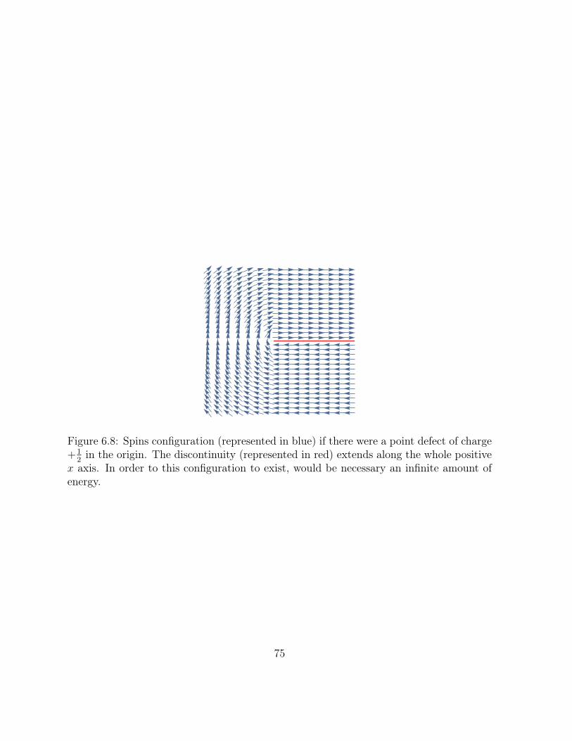
Figure 6.8: Spins configuration (represented in blue) if there were a point defect of charge+1

2in the origin. The discontinuity (represented in red) extends along the whole positive

x axis. In order to this configuration to exist, would be necessary an infinite amount ofenergy.

75

Bibliography

Geometry and Topology

[A1] A. Hatcher, Algebraic Topology. Cambridge University Press, 2009.

[A2] B. O’neill, Elementary differential geometry. Elsevier, 2 ed., 2006.

[A3] A. Pressley, Elementary Differential Geometry. Springer, 2010.

[A4] M. Carmo, Riemmanian Geometry. Birkhäuser, 1992.

[A5] M. D. Carmo, Differential geometry of curves and surfaces. Pearson, 1976.

[A6] J. Lee, Introduction to Topological Manifolds. Springer, 2010.

[A7] J. Lee, Introduction to Smooth Manifolds. Springer, 2012.

[A8] J. Lee, Riemannian Manifolds: An Introduction to Curvature. Springer, 1997.

Applications in Physics

[B9] M. Nakahara, Geometry, topology and physics. CRC Press, 2003.

[B10] J. Cornwell, Group Theory in Physics: An Introduction. Academic Press, 1997.

[B11] R. Kamien, “The geometry of soft materials: a primer,” Reviews of Modern Physics,vol. 74, no. October, 2002.

76

[B12] P. Szekeres, A Course in Modern Mathematical Physics: Groups, Hilbert Space andDifferential Geometry. Cambridge University Press, 2004.

[B13] J. Baez and J. Muniain, Gauge Fields, Knots and Gravity. World Scientific Pub-lishing Company, 1994.

Condensed Matter and Topological Defects

[C14] H. Trebin, “The topology of non-uniform media in condensed matter physics,” Ad-vances in Physics, 1982.

[C15] M. Kleman and J. Friedel, “Disclinations, dislocations and continuous defects: areappraisal,” Reviews of Modern Physics, p. 72, apr 2007.

[C16] D. Ruppel and E. Sackmann, “On defects in different phases of two-dimensionallipid bilayers,” Journal de Physique, 1983.

[C17] V. Poénaru, “Some aspects of the theory of defects of ordered media and gauge fieldsrelated to foliations,” Communications in mathematical physics, vol. 136, pp. 127–136, 1981.

[C18] P. Chaikin and T. Lubensky, Principles of condensed matter physics. CambridgeUniversity Press, 2000.

[C19] P. D. Gennes and J. Prost, The physics of liquid crystals. Oxford University Press,1993.

[C20] M. Kleman and O. D. Lavrentovich, Soft Matter Physics: An Introduction. Par-tially Ordered Systems, New York, NY: Springer New York, 2004.

[C21] N. Mermin, “The topological theory of defects in ordered media,” Reviews of ModernPhysics, no. 3, 1979.

[C22] M. Kurik and O. Lavrentovich, “Defects in liquid crystals: homotopy theory andexperimental studies,” Soviet Physics Uspekhi, vol. 196, 1988.

77