Digital Comprehensive Summaries of Uppsala Dissertationsfrom the Faculty of Science and Technology 21

Theoretical Studies of Two-Dimensional Magnetism and Chemical Bonding

OLEKSIY GRECHNYEV

ISSN 1651-6214ISBN 91-554-6164-6urn:nbn:se:uu:diva-4815

ACTAUNIVERSITATIS

UPSALIENSISUPPSALA

2005

ISBN

65

Dedicated to Gary Gygax, Dave Arne-son, George Lucas and Bioware Corp.

List of Papers

This thesis is based on the following papers, which are referred to in the textby their Roman numerals.

I Thermodynamics of a two-dimensional Heisenberg ferromag-net with dipolar interactionA. Grechnev, V. Yu. Irkhin, M. I. Katsnelson and O. ErikssonPhys. Rev. B. 71, 024427 (2005).

II Geometry of the valence transition induced surface reconstruc-tion of Sm(0001)E. Lundgren, J. N. Andersen, R. Nyholm, X. Torelles, J. Rius,A. Delin, A. Grechnev, O. Eriksson, C. Konvicka, M. Schmid, P.VargaPhys. Rev. Lett. 88, 136102 (2002).

III Balanced crystal orbital overlap population-a tool for analysingchemical bonds in solidsA. Grechnev , R. Ahuja and O. ErikssonJ. Phys.: Condens. Matter 15, 7751 (2003).

IV A new nanolayered material, Nb3SiC2, predicted from First-Principle s TheoryA. Grechnev, S. Li, R. Ahuja, O. Eriksson, U. Jansson and O.WilhelmssonAppl. Phys. Lett. 85, 3071 (2004).

V Elastic properties of Mg1−xAlxB2 from first principles theoryP. Souvatzis, J. M. Osorio-Guillen, R. Ahuja, A. Grechnev andO. ErikssonJ. Phys.: Condens. Matter 16, 5241 (2004).

VI H-H interaction and structural phase transition in Ti3SnHx

A. Grechnev, P. H. Andersson, R. Ahuja, O. Eriksson, M. Vennströmand Y. AnderssonPhys. Rev. B 66, 235104 (2002).

VII Phase relations in the Ti3SnD systemM. Vennström , A. Grechnev , O. Eriksson and Y. AnderssonJ. Alloy. Compd. 364, 127 (2004).

v

Reprints were made with permission from the publishers.

The following papers are not included in the thesis

I Ab initio calculation of depth-resolved optical anisotropy ofthe Cu(110) surfaceP. Monachesi, M. Palummo, R. Del Sole, A. Grechnev and O.ErikssonPhys. Rev. B 68, 035426 (2003).

II Unusual magnetism and magnetocrystalline anisotropy of CrPt3P. M. Oppeneer, I. Galanakis, A. Grechnev and O. ErikssonJ. Magn. Magn. Mater. 240, 371 (2002).

III Many-body projector orbitals for electronic structure theoryof strongly correlated electronsO. Eriksson, J.M. Wills, M. Colarieti-Tosti, S. Lebégue and A.GrechnevSubmitted to Int. J. Qu. Chem.

Comments on my contribution

In the papers where I am the first author I am responsible for the main part ofthe work: theory, calculations and writing the paper. In the other papers I havecontributed in different ways, such as ideas, calculations, code developmentor analysis.

vi

Contents

1 Introduction . . . . . . . . . . . . . . . . . . . . . . . . . . . . . . . . . . . . . . . . . . 12 Thermodynamics of a 2D ferromagnet with dipolar interaction . . . . 5

2.1 Heisenberg model . . . . . . . . . . . . . . . . . . . . . . . . . . . . . . . . . . 72.2 Magnons and Mermin-Wagner theorem . . . . . . . . . . . . . . . . . . 102.3 Free magnons with dipolar interaction . . . . . . . . . . . . . . . . . . . 132.4 Self-consistent spin-wave theory . . . . . . . . . . . . . . . . . . . . . . . 192.5 Calculation of the lattice sums: Ewald method . . . . . . . . . . . . . 252.6 SSWT results . . . . . . . . . . . . . . . . . . . . . . . . . . . . . . . . . . . . . 26

3 Interlude: Density functional theory . . . . . . . . . . . . . . . . . . . . . . . . 333.1 Hohenberg-Kohn theorem . . . . . . . . . . . . . . . . . . . . . . . . . . . . 343.2 Kohn-Sham equation . . . . . . . . . . . . . . . . . . . . . . . . . . . . . . . . 353.3 The FP-LMTO method . . . . . . . . . . . . . . . . . . . . . . . . . . . . . . 393.4 Pseudopotentials and the OPW method . . . . . . . . . . . . . . . . . . 403.5 Projector Augmented-Wave (PAW) method . . . . . . . . . . . . . . . 443.6 Quasiparticle excitations vs Kohn-Sham eigenvalues . . . . . . . . 45

4 Balanced crystal orbital overlap population (BCOOP) . . . . . . . . . . 494.1 Definition of COOP and COHP . . . . . . . . . . . . . . . . . . . . . . . . 494.2 Orbital population of an H2-like molecule . . . . . . . . . . . . . . . . 514.3 Definition of BCOOP . . . . . . . . . . . . . . . . . . . . . . . . . . . . . . . 524.4 BCOOP for Si, TiC, Ru, Na and NaCl . . . . . . . . . . . . . . . . . . . 534.5 Nb3SiC2 – a theoretically predicted new MAX phase . . . . . . . . 594.6 Chemical bonding in MgB2 . . . . . . . . . . . . . . . . . . . . . . . . . . . 62

5 Hydrogen–hydrogen interaction and structural stability of Ti3SnHx 655.1 Hydrogen-metal and hydrogen-hydrogen interactions . . . . . . . 665.2 Ti3SnHx as a model system . . . . . . . . . . . . . . . . . . . . . . . . . . . 675.3 The H–H pair potential . . . . . . . . . . . . . . . . . . . . . . . . . . . . . . 705.4 Physics behind the H–H repulsion . . . . . . . . . . . . . . . . . . . . . . 73

6 Sammanfattning på svenska . . . . . . . . . . . . . . . . . . . . . . . . . . . . . . 77

vii

1 Introduction

What is physics? The best definition I can come up with is "Physics is the partof natural science which is not chemistry, biology, geology or any other disci-pline". And, I must add, physics uses a lot of math, in contrast to philosophy.So, physics studies everything about the world, except for the things belong-ing to other sciences. Physics also includes many branches: particle physics,solid state (or condensed matter) physics, nonlinear dynamics etc. This thesisonly deals with the solid state physics.

Physics is divided into experimental, theoretical and computational physics.Experimental physics is the oldest kind of physics. It started with our everydayexperience (an apple falls onto your head), and later evolved into true experi-ment (shake the apple tree to achieve certain effect). Theoretical physics usesmathematical language to systemathize experimental data. Modern physicscould not exist without precisely defined experimentally meauserable quanti-ties (e.g. velocity, mass, resistivity), precisely defined but not directly mea-surable ones (e.g. entropy, wave function), and also more intuitive, qualitativeconcepts (e.g. chemical bonding). We need this language to understand theresults of any modern experiment (or even to perform one). With our appleexample, we must first define mass, force and distance in order to come upwith Newton’s law of gravity. A physical law is a generalization of the exper-imental data, usually written as a mathematical equation, which we believe tobe valid under certain circumstances.

Once the laws are established, the true theoretical physics begins. The pointis to predict new results from known laws without doing the experiment. Inthe process, new concepts, formalisms and even new laws are created. Whenwe cannot get result with pen and paper, the computational physics, histori-cally the latest of the three, comes into play. Computational physics is basedon quantum mechanics. The Schrödinger equation for the nonrelativistic caseand Dirac equation in the relativistic case are the basic equations of quan-tum mechanics. In principle, they describe all matter, from nuclei to galaxies.However, quantum-mechanical description employs wavefunction Ψ whichdepends on coordinates of all particles of the system. For solids, the numberof particles N is of the order of 1023. Even the best supercomputers cannottreat functions depending on 1023 variables. The revolution in computationalphysics happened in 1960’s when the theory known as the Density Functional

1

Theory (DFT) was developed. DFT uses the particles density n(r) which de-pends only on 3 variables instead of 3N variables. DFT is the foundation ofmodern computational physics. Like in experiment, the end result of a compu-tation is a bunch of numbers. The most interesting part of the computationalwork is analysis of the results, and it always involves a bit of theory.

Physical science works best when theoretical, experimental and computa-tional physics all work together, compare their results all the time (and findthem to disagree, which is the normal situation in practical work). It is really apity when theorist, experimentalist and computationalist speak only their ownlanguage and don’t understand each other.

I do not perform any experiments. My work lies in between theory andcomputation: while performing calculations I create simple theoretical mod-els whenever I need them. These “theoretical miniatures” are not as big andimportant as quantum mechanics or general relativity, but they suit well theproblems I am trying to solve.

The first part of my thesis is devoted to the magnetism of two-dimensional(2D) systems. A 2D magnet is the heart of any magnetic data recording. Ourwork is based not on DFT but on the model Hamiltonian called HeisenbergHamiltonian. We have studied thermodynamics of a 2D ferromagnet with thelong-range dipolar interaction, namely we wanted to know the magnetizationcurve M(T ) and the Curie temperature Tc. The existing theoretical approacheswere found to be insufficient for the task. Our task was to construct a for-malism to treat both classical and quantum Heisenberg models with dipolarinteraction. Note that for 2D systems one should use quantum and not clasicalHeisenberg model even for large spins such as S = 7/2.

The second part of my thesis deals with the problem of describing chemicalbonding from the first principles. Chemical bonding is the force that holdsmolecules and solids together. Basically, it always comes from the Coulombattraction between electrons and nuclei, however, in solids it can take manyforms: covalent bonding, metallic bonding, ionic bonding etc. When study-ing a solid, it is very important to know the precise nature of the chemicalbonding. We have found that existing chemical bonding indicators (COOP,COHP) do not work well with full-potential DFT methods. Therefore, we haddo develop a less basis set dependent indicator which we now call BalancedCrystal Orbital Overlap Population (BCOOP). The test calculations for dif-ferent systems (Si, Ru, TiC, Na and NaCl) with BCOOP has been performed.

We have also applied BCOOP to a possible new MAX phase Nb3SiC2.MAX phases are newly discovered layered materials with a great ability towithstand thermal shock and other unique propeties. Our calculation showthat Nb3SiC2 is unstable, but the formation energy is only about 0.2 eV/atom,therefore its existence in metastable form is likely. Another BCOOP exampleis MgB2, a recently discovered superconductor with Tc = 39 K. This com-

2

pound is unique since it combines covalent, ionic and metallic bonding in asingle solid.

Another project involves hydrogen–hydrogen interaction in metals. It isknown that H atoms in a metal repel each other at short distances, with theminimal H–H distance being about 2Å. For the hydrogen storage applica-tions, however, the materials with small H–H distances are desired. We haveanalyzed the H–H interaction using the pair-potential model. By the exampleof Ti3SnHx we have studied how the H–H interaction stems from the metal–hydrogen chemical bonding and how it can be responsible for structural phasetransitions in metal hydrides.

3

2 Thermodynamics of a 2D ferromagnet withdipolar interaction

In the early 80’s the ultrathin magnetic films and magnetic multilayers be-came a very active field of research[1]. Surprisingly, they are still a hottopic in 2005. That means that these two-dimensional (2D) magnetic sys-tems have important technological applications. Indeed, such systems notonly form the media of every hard disc, but also can be found in the read/writeheads of the same disc. They are also crucial for the relatively novel field ofspintronics[2, 3]. All these technological achievements stem from the uniquephysical properties of the 2D magnetic systems. For example, magnetic mul-tilayers demonstrate oscillating exchange coupling [4] and giant magnetore-sistance (GMR)[5]. Many people believe that GMR is the most importantdiscovery in physics in the last 50 years.

Superlattice

2D Quasi−2D

Multilayer

Figure 2.1: Cross section of different 2D and quasi-2D lattices.

But what is a 2D lattice? What is a quasi-2D lattice? Different types of 2Dand quasi-2D crystal lattices are shown in Fig. 2.1 in the “cross section”. A2D lattice is simply a crystal lattice periodical in two dimensions and confinedin the third dimension. It is known that 2D and 1D crystals cannot be stable atnonzero temperature. Nature tries to find the equilibrium by folding the low-

5

D crystal. Indeed, 2D carbon sheets fold into fullerenes, while 1D polymermolecules (including proteins and DNA) fold into spirals and even more com-plicated structures. How can thin films (which are 2D systems) exist in reallife then? The answer is that this theorem applies only to infinite 2D crystals,while stable films have finite size and they are also sufficiently thick (as com-pared to their other dimensions). Really thin films, on the other hand, mustbe deposited on a thicker substrate. One particular type of 2D lattice is themultilayer, which consists of several layers of different materials. A quasi-2Dlattice is, strictly speaking, 3D and not 2D lattice. However, its layered crystalstructure is strongly anisotropic. As a result, certain interactions (e.g. the ex-change interaction responsible for the magnetism) are much stronger withineach atomic layer than between the layers. In other words, the systems be-haves like an array of 2D crystals only weakly interacting with each other. Aspecial case of the quasi-2D lattice is the superlattice, the periodic multilayer.

The Heisenberg model is the most common theoretical model for magneticmaterials. It can describe dynamics and thermodynamics of a magnetic sys-tem, in particular, we can calculate the magnetization curve M(T ) and theCurie temperature Tc. The spin variable on each lattice site can be either clas-sical or quantum, therefore we speak of the classical Heisenberg model andthe quantum Heisenberg model. The Heisenberg model, in general, has noexact solution. Therefore we need either a direct numerical solution (MonteCarlo method), or some sort of approximation.

It is known (Mermin-Wagner theorem[6]) that 2D and 1D magnetic sys-tems cannot have any long-range magnetic order at T > 0, provided that onlyan isotropic, short-range exchange interaction is included (not a big surprise,really, when even the crystal lattice is unstable). In real life even low-D mag-nets still have a finite Tc (although it is generally lower than the Tc of the corre-sponding bulk materials). One reason for this is the finite size effect describedabove. A more common reason is that the magnetocrystalline anisotropy andthe dipolar interaction, despite being “small”, have a crucial effect on the1D or 2D system by breaking the conditions of the Mermin-Wagner theo-rem. Moreover, the latter interaction has a strong effect on spin waves in thinfilms[7, 8]. The competition between perpendicular anisotropy and the dipolarinteraction often results in the reorientation transition[9]. While it is relativelyeasy to include anisotropy in most theoretical approaches to the Heisenbergmodel, the dipolar interaction presents much more challenge. While the clas-sical 2D Heisenberg model with the dipolar interaction has been studied ratherextensively[10–19], the quantum results are scarce. To the best of our knowl-edge, the only approaches applied in the quantum case are spin-wave theory(free magnons) [20–22] and Tyablikov approximation [23, 24]. The motiva-tion of the present work (Paper I) is to study the latter case (thermodynamicsof a quantum 2D Heisenberg model with dipolar interaction) in more detail.

6

The chosen formalism is the self-consistent spin-wave theory (SSWT), whichdid not include dipolar interaction until the present work.

Paper II presents a completely different approach to the 2D magnetism.Besides experimental results, it includes a density functional theory calcultionof the samarium surface. It is included in the thesis to illustrate the variety ofmethods applied to the 2D magnetic systems.

2.1 Heisenberg modelThere is no single model which would describe all magnetic systems and coverall physical effects. The Heisenberg model (see e.g. [25, 26]) is a simpletheoretical model for a magnetic solid. This model assumes that each latticesite i, located at position Ri, bears a localized magnetic moment, described bya quantum-mechanical spin operator Si (or total angular momentum operatorJi).

The Heisenberg Hamiltonian consists of up to four terms

H = Hex +Han +Hdd −h∑i

Si. (2.1)

Let us look at each one in turn.The exchange term has the form

Hex = −12 ∑

i= jJi jSiS j, (2.2)

where Ji j is called exchange integral. There are various mechanisms for thisinteraction[25], and it is normally a short-range one, i.e. Ji j should decreasesufficiently fast with distance Ri j ≡ Ri −R j. Positive, or ferromagnetic, Ji j

favours parallel spin alignment, while the negative, or antiferromagnetic, Ji j

favours antiparallel spin alignment (although the AFM ground state is a diffi-cult problem by itself). One needs to include exchange interaction with manyneighbor shells (sometimes 100 or more) to describe magnetic solids quanti-tatively. However, theorists often study simpler models with only one or twoshells included.

The exchange term is isotropic in the sense that it is invariant under anyrotation applied to each and every spin in the system. Indeed, if the same ro-tation is applied to Si and S j, then the scalar product SiS j does not change.Therefore, directions in the spin space are completely uncoupled to the direc-tion of the crystal lattice. This symmetry is broken by the anisotropy term,which can have various forms, for example

Han = −K ∑i

(Szi )

2 (2.3)

7

is called single-ion quadratic uniaxial anisotropy. Anisotropy comes from therelativistic effect called spin-orbit interaction.

The dipolar, or magnetostatic term

Hdd = −12 ∑

i= jQαβ

i j Sαi Sβ

j , (2.4)

whereQαβ

i j = Jd

(3Rα

i jRβi j −δαβ R2

i j

)R−5

i j , (2.5)

describes the magnetostatic interactions between two magnetic moments. Thisis essentially the same effect as the interaction between two permanent mag-nets. The interaction constant Jd is equal to Jd ≡ (gµb)2), where µb is the Bohrmagneton, and g is the gyromagnetic ratio (g = 2 for spin magnetic moments).If we chose to measure length in the units of a, with a of the order of the latticeconstant, then vectors Ri j become unitless, and Jd = (gµb)2/a3 will have thesame dimension as Ji j (energy). However, dipolar interaction is a long rangeone (namely it decreases as R−3). It leads to new physical effects even thoughnormally Jd is much smaller than the nearest-neighbor exchange integral.

The last term is simply the Zeeman coupling to the external magnetic fieldH, and h ≡−gµbH.

To summarize, the Heisenberg model assumes that• The magnetic moment at each site is localized• It comes from a single quantum-mechanical spin operator S (or total angu-

lar momentum operator J), and the spin value S is the fixed parameter ofthe model.This model is applicable to most f-electron magnets (although one might

need to use total angular momentum J instead of the spin S), most insulating d-electron magnets, and (to less extent) many metallic d-electron magnets (suchas iron). However, other metallic d-electron magnets (such as nickel) havepoorly localized magnetic moments. The picture opposite to the Heisenbergmodel is the itinerant picture, which considers the magnetism of nearly-freeband electrons.

The classical Heisenberg model uses classical spin (a fixed-length vector)instead of the quantum-mechanical spin operator. It is often said that the clas-sical model is valid if S 1, however, this is not always true. We are going tocome back to this question soon.

As we have mentioned above, the exact solution of the Heisenberg model isnot known, and various approximations are used. Some approximations havelimited applicability: for example they can be used only for classical model, oronly for 2D lattices, or only for the model without dipolar interaction. Thereare several classes of approximate theories, which we are now going to men-tion briefly, focusing on the theories most suitable for the 2D systems.

8

Monte Carlo methods are formally exact and give a numerical solutionto the Heisenberg model with any desired accuracy. Quantum Monte Carlo(QMC) calculations have been carried out for small values of spin (such asS = 1/2 and S = 1) for 2D systems [27–30], as well as for 3D systems. QMCcalculations are quite resource demanding and they are not yet available forlarger values of spin or for the Heisenberg model with a dipolar term. Classi-cal Monte Carlo calculations are less time consuming and they are availableeven for 2D systems with dipolar interaction [11, 12, 15–17, 19]. A very in-teresting theory called pure-quantum self-consistent harmonic approximation(PQSCHA)[31, 32] gives a quantitative solution to the quantum Heisenbergmodel with a computational effort comparable to that of a classical MonteCarlo calculation (but no dipolar interaction yet).

One group of approximate theories is based on magnon operators (magnonsare interacting bosons, the quanta of spin waves), introduced via Dyson-Maleev,Holstein-Primakoff, or some other bosonic transformation. In the next twosections I am going to speak about magnons and discuss the problem of ex-tra states. Free-magnon (spin-wave, SW) theory is only a very rough startingpoint that normally overestimates Tc by a factor of 2–4. In order to get betterresults, we must take magnon-magnon interaction into account. Interactingmagnon theories use various small parameters, such as temperature, 1/S or1/N of the SU(N) model1. The magnon-magnon interaction is often treatedas a perturbation and sometimes the Feynman diagram technique is used formagnons. In two dimensions, the most useful magnon-based theory is theso-called self-consistent spin-wave theory (SSWT). It was first formulated forthe Mermin-Wagner situation [33–36], but it was later generalized to systemswith long-range order [37, 38]. SSWT can be formulated as the best possibleone-magnon theory [35, 38], the zeroth order term in the 1/N expansion ofthe SU(N) theory [36, 39] or as the mean-field magnon theory [38]. Note thathere and in the following the words “mean field” are applied to magnon occu-pation number operators and have nothing to do with the Weiss mean field forspin operators. Loosely speaking, SSWT can be called “Hartree-Fock theoryfor magnons”. The SSWT result can be further improved by renormalizingthe magnon-magnon vertex[38], often providing quantitative agreement withexperiment everywhere except the narrow critical region2. The known weakpoint of SSWT is the erroneous critical behavior in the vicinity of the phasetransition: SSWT gives either a spin-wave second-order phase transition with

1 Rotations in the spin space (for any S) are given by the SU(2) group. Different values ofspin correspond, therefore, to different representations of SU(2). SU(N) model generalizes theconcept of spin and the Heisenberg model by using the SU(N) group instead. 1/N theories use1/N as a formal small parameter and then put N = 2 in the final equations.2This approximation is often called the random phase approximation (RPA). Again, do notconfuse with “RPA” for spin operators, which is the Tyablikov approximation.

9

β = 13, or a first-order transition (β = 0). However, SSWT describes per-fectly the wide region of the short-range order (SRO) above Tc [40], which isthe unique feature of low-D systems. Until our work, the SSWT formalismdid not include dipolar interaction.

Another group of theories is based directly on spin operators, without in-troducing any magnon operators. The simplest one is the Weiss mean-fieldtheory. This theory is not good enough for low-D systems, since it is notconsistent with the Mermin-Wagner theorem. Instead, it gives Tc of the or-der of JS2 (from now on we measure temperature in the energy units). Otherwell-known approximations based on spin operators are Tyablikov[41] andAnderson-Callen[42] decouplings. There is even a perturbation theory forspin operators. But this time the unperturbed system is just the lattice of un-coupled spins in the external magnetic field, while all spin-spin interactions(including the exchange) are treated as perturbations. There is no Wick’s the-orem for spin operators, therefore it is much more difficult to build Feynmandiagram technique for spin operators than for magnon operators.

2.2 Magnons and Mermin-Wagner theorem

The most important elementary excitations of the Heisenberg model are magnons,the quanta of spin waves. Consider, for example, the ferromagnet with allspins pointing along the z axis in the ground state. In the Heisenberg represen-tation of the quantum mechanics, spin dynamics is described by the equationof motion

dS j

dt=

ih

[H,S j] . (2.6)

With the notationS±j = Sx

j ± iSyj, (2.7)

we seek the single-magnon solution of the form[25]

S−j =A√N

ei(ωkt+kR j) (2.8)

With the exchange-only Heisenberg Hamiltonian, the magnon energy as func-tion of k (dispersion law) is

Ek ≡ hωk = S (J0 − Jk) , (2.9)

3β is the critical exponent in the magnetization vs temperature dependence: M(T ) ∼ (Tc −T )β

when T → Tc −0

10

whereJk ≡ ∑

ie−ikRi Joi. (2.10)

Alternatively, this result can be obtained by the method of the next section(Holstein-Primakoff transformation).

There is one big difference between magnetism in 3D and 2D systems. The3D Heisenberg model always has long-range magnetic order at sufficientlylow temperatures, with a transition temperature of the order of JS2, whereJ is a typical value of the exchange integral. However, the Mermin-Wagnertheorem[6] states that no 2D or 1D Heisenberg system can have long-rangeorder at T > 0, provided that only isotropic short-range exchange interactionis included. Although the theorem can be proven rigorously, here we onlypresent the simple explanation of this phenomenon given by Bloch[43] longbefore the paper by Mermin and Wagner.

If the temperature is sufficiently low, the magnons can be approximatelytreated as independent bosons (free magnon theory). In that case, the magne-tization is given by

〈Sz〉 = S− 1VBZ

∫BZ

dkexp(Ek/T )−1

. (2.11)

The magnon energy (2.9) is proportional to k2 for small k, for example Ek ≈JSk2 for nearest-neighbor only exchange. For the 3D Heisenberg model

dkexp(Ek/T )−1

≈ 4πk2dkT

JSk2 , (2.12)

and the integral in (2.11) converges at small k, giving a finite number ofmagnons at low T . In two dimensions however, this is not the case. Namely,for small k

dkexp(Ek/T )−1

≈ 2πkdkT

JSk2 , (2.13)

thus the integral in (2.11) diverges logarithmically at the lower limit. Thismeans that the magnetic order breaks down at temperature above zero.

This result directly contradicts the experiment. In real life even 1D and2D magnetic systems have finite Tc. The reason for this is the presence ofadditional interactions (anisotropy, dipolar interaction or interlayer exchangein quasi-2D systems), and also the finite size of the sample. Each of thesefactors breaks the conditions of the Mermin-Wagner theorem (see e.g. Ref.[38]), resulting in a finite Tc JS2. It is interesting that the short-range order,does not disappear at or close to Tc, as for the 3D systems, but stays up toT ∼ JS2 (Ref. [40]) for the low-D systems.

In terms of Eq. (2.11) any of the additional interactions mentioned above

11

makes the integral (2.11) convergent in 2D. The easy-axis anisotropy simplyintroduces a gap JS∆ in the magnon spectrum, while for the dipolar interactionthe situation is a bit more complicated (see below). In all cases we can intro-duce the "effective gap", or low energy cutoff ∆ 1 and the magnetization isgiven by (for a 2D square lattice)

S−〈Sz〉 ≈ T4πJS

∫ T

JS∆

dEE

=T

4πJSln(

TJS∆

), (2.14)

giving a spin-wave expression for Tc

Tc ≈ 4πJS2

ln(Tc/JS∆) 4πJS2. (2.15)

Thus Tc in the 2D case is indeed much smaller than in the 3D case, so we canstill speak of the "Mermin-Wagner scenario". If we seek an approximate solu-tion to the Heisenberg model, we must be sure that the approximation used isconsistent with the Mermin-Wagner theorem. Some approximations, for ex-ample Weiss mean-field model, give finite Tc even for 1D and 2D systems.Therefore these approximations cannot be applied to the low-dimensionalcase. In order to give the Mermin-Wagner behavior, the approximation inquestion must have a correct form of magnon dispersion law at low T andk → 0.

We are now back to the question of applicability of the classical Heisenbergmodel. First note that the upper integration limit in Eq. (2.14) comes from theBose function, and it is equal to T only for the quantum model with T JS.For the classical model, or for the case T JS, the Bose function can be re-placed by T/E and the upper limit is equal to 32JS, the value that stems fromthe finite size of the Brillouin zone. The classical description is thus appro-priate if the Curie temperature is much larger than any spin-wave frequency,namely if Tc JS. For the 3D Heisenberg model Tc ∼ JS2, and this criteriontakes the well-known form S 1. That is why the classical Heisenberg modelis immensely useful for the 3D systems, especially for the Monte-Carlo cal-culations. However, for the 2D Heisenberg model Tc JS2, and the classicaldescription is only valid if S ln(1/∆) 1 (see Ref. [38]). This does nothold even for the largest spins such as S = 7/2, therefore the quantum effectsare never negligible for 2D magnetic systems, at least for a single monolayer.However, if we increase film thickness, there is a crossover from 2D to 3Dbehavior, and the classical description gets better.

12

2.3 Free magnons with dipolar interaction

Now that the long introductory part is over, it is time to formulate the model ofPaper I, which this chapter is based upon. We consider the quantum Heisen-berg model on the simple 2D square lattice in the xz plane with lattice constanta. We include nearest-neighbor ferromagnetic exchange J and the dipolar in-teraction Jd = (gµb)2/a3 (and no anisotropy or Zeeman terms for simplicity).As in the previous sections, we take the lattice constant a to be the unit oflength. If Jd is sufficiently small, the ground state is ferromagnetic with an xzeasy plane, and we take the z-axis direction for the ground state magnetization.The parameters of the model are therefore J, Jd , S (the value of spin) and T(temperature). The goal of this section is to study this model within the free-magnon (spin-wave) approximation. This has been first done by Maleev[20].The spin-wave theory is only valid at T Tc and normally gives a very badvalue for Tc, however this is a reasonable place to start.

The Hamiltonian (2.1) becomes

H = Hex +Hdd = −12 ∑

i= j

(Ji jδαβ +Qαβ

i j

)Sα

i Sβj , (2.16)

whereQαβ

i j = Jd

(3Rα

i jRβi j −δαβ R2

i j

)R−5

i j . (2.17)

With the notation (2.7) the scalar product SiS j is equal to

SiS j =12

(S+

i S−j +S−i S+j

)+Sz

i Szj, (2.18)

and the exchange term becomes

Hex = −12 ∑

i= jJi jSiS j = −1

2 ∑i= j

Ji j

[12

(S+

i S−j +S−i S+j

)+Sz

i Szj

]=

− 12 ∑

i= jJi j

[S−i S+

j +Szi S

zj

], (2.19)

since we can always assume Jji = Ji j.

13

The dipole-dipole part is equal to

Hdd =12

Jd ∑i= j

R−3i j

[S−i S+

j +Szi S

zj

]−

32

Jd ∑i= j

R−5i j

(Sz

i Zi j +12

S+i R−

i j +12

S−i R+i j

)(Sz

jZi j +12

S+j R−

i j +12

S−j R+i j

)=

12

Jd ∑i= j

R−3i j

[S−i S+

j +Szi S

zj

]− 3

2Jd ∑

i= jR−5

i j

Sz

i SzjZ

2i j +

12

R+i jR

−i jS

−i S+

j +

14

(R−

i j

)2S+

i S+j +

14

(R+

i j

)2S−i S−j +S+

i SzjR

−i jZi j +S−i Sz

jR+i jZi j

, (2.20)

whereR±

i j ≡ Xi j ± iYi j. (2.21)

Combining Eqs. (2.19) and (2.20) gives

H = ∑i= j

Φ0

i jS−i S+

j +Φzi jS

zi S

zj +Φ−

i jS+i S+

j +Φ+i jS

−i S−j +Φz−

i j S+i Sz

j +Φz+i j S−i Sz

j

,

(2.22)where

Φ0i j ≡−Ji j

2− 1

4JdR−3

i j

[1−3

Z2i j

R2i j

], (2.23)

Φzi j ≡−Ji j

2+

12

JdR−3i j

[1−3

Z2i j

R2i j

], (2.24)

Φ±i j ≡−3

8Jd

(R±

i j

)2

R5i j

, (2.25)

Φz±i j ≡−3

2Jd

R±i jZi j

R5i j

. (2.26)

The expression (2.22) is, in fact, still valid for any 2D or 3D crystal lattice,but from now on we restrict ourselves to the 2D square net.

After the Fourier transform

Sαk =

1√N ∑

Ri

e−ikRiSαi , Sα

i =1√N ∑

keikRiSα

k , (2.27)

14

with

∑k≡V

∫ d2k(2π)2 , ∑

k1 = N, (2.28)

the Hamiltonian becomes

H = ∑k

Φ0

kS−k S+−k +Φz

kSzkSz

−k +Φ−k S+

k S+−k

+ Φ+k S−k S−−k +Φz−

k S+k Sz

−k +Φz+k S−k Sz

−k

, (2.29)

where various Φk are Fourier transformed versions of respective Φi j

Φk = ∑Ri =0

e−ikRiΦ0i, Φi j =1N ∑

keik(R j−Ri)Φk. (2.30)

They are equal to

Φ0k = −Jk

2− 1

4Jd

[S1(k)− 1

2S3

], (2.31)

Φzk = −Jk

2+

12

Jd

[S1(k)− 1

2S3

], (2.32)

Φ+k = Φ−

k = −38

Jd

[S2(k)+

12

S3

], (2.33)

Φz+k = Φz−

k = −32

Jd ∑Ri =0

eikRiXiZi

R5i

, (2.34)

where three lattice sums have been introduced

S3 ≡ ∑Ri =0

R−3i ≈ 9.034 , (2.35)

S1(k) ≡ ∑Ri =0

(eikRi −1

)R−3

i

[1−3

Z2i

R2i

], (2.36)

S2(k) ≡ ∑Ri =0

(eikRi −1

) X2i

R5i, (2.37)

andJk ≡ ∑

ie−ikRi Joi. (2.38)

15

For the nearest neighbor exchange Jk is equal to 2J coskx + 2J coskz. Fromnow on and to the rest of this chapter our general equations are valid for anyform of Ji j (and therefore Jk), but all asymptotics and numerical results arepresented for the nearest-neighbor exchange. For small k the lattice sums(2.36),(2.37) have the asymptotical form

S1(k) ≈ 2πk2

z

k, S2(k) ≈−2

3πk

(2k2

z + k2x). (2.39)

Remember that the particular expressions for the different Φk-s and latticesums above are only valid for the simple square lattice.

Now we formally introduce magnons by the Holstein-Primakoff transfor-mation

S+i =

√2S(

1−a†i ai/2S

)1/2ai (2.40)

S−i =√

2Sa†i

(1−a†

i ai/2S)1/2

(2.41)

Szi = S−a†

i ai, (2.42)

and expand the Hamiltonian (2.16) into the series of S−1/2

H = S2N0 +S1N2(a†k,ak)+S1/2N3(a†

k,ak)

+S0N4(a†k,ak)+S−1/2N5(a†

k,ak)+ . . . , (2.43)

where Nn(a†k,ak) means a certain n-th order polynomial of the Bose operators

a†k, ak in the normal form (creation operators to the left). This expansion gives

rise to the problem of extra states (with 〈Sz〉 < −S) and it does not work at allfor e.g. systems with easy-plane anisotropy. The problem of extra states hasbeen studied in Ref. [38] using pseudo-fermions and was found to be notcrucial for most 2D systems. The question of convergence of the series (2.43)is irrelevant since we are only using terms up to N4 in SSWT (see below).

The free-magnon Hamiltonian is

H0 ≡ S1N2(a†k,ak)−µ ∑

ka†

kak

= ∑k

A0

ka†kak +

12

B0ka†

ka†−k +

12

B0kaka−k

, (2.44)

where

A0k = S(J0 − Jk)− 1

2JdS[

S1(k)− 32

S3

]−µ (2.45)

16

and

B0k = −3

2JdS[

S2(k)+12

S3

]. (2.46)

The “magnon chemical potential” µ is the Lagrange multiplier used in spin-wave theory and SSWT to enforce the condition < Sz >≡ S = 0 in the para-magnetic (PM) phase (in the ferromagnetic phase one has µ = 0). The nextstep is to get rid of the “anomalous” terms a†

ka†−k and aka−k by the Bogoliubov

transformation ak = cosh(ξk)bk − sinh(ξk)b†

−k

a†k = cosh(ξk)b†

k − sinh(ξk)b−k(2.47)

with

tanh(2ξk) =B0

kA0

k. (2.48)

The Hamiltonian in the new magnon operators b†k,bk has a trivial free-

bosons form

H0 = const+∑k

ε0kb†

kbk , ε0k =√(

A0k)2 − ∣∣B0

k∣∣2, (2.49)

therefore the thermodynamic average number of the “new magnons” is givensimply by the Bose function⟨

b†kbk

⟩= Nk ≡ [exp(ε0

k/T )−1]−1

. (2.50)

The thermodynamic averages involving the “old magnon” operators are foundusing the Bogoliubov transformation (2.47)⟨

a†kak

⟩=

A0k

ε0k

(⟨b†

kbk

⟩+

12

)− 1

2, (2.51)

⟨a†

ka†−k

⟩= 〈aka−k〉 = −B0

kε0

k

(⟨b†

kbk

⟩+

12

). (2.52)

Alternatively, the expectation value (2.51) can be obtained from the free-magnon Matsubara Green’s function (as it has been done in Ref. [20])

G0k(iωn) =

iωn +A0k

(iωn)2 − (ε0

k)2 , ωn ≡ 2πnT (2.53)

17

through the frequency summation⟨a†

kak

⟩= lim

τ→+0T ∑

iωn

eiτωnG0k(iωn). (2.54)

If Jd = 0, then B0k = 0 and A0

k = ε0k is given by Eq. (2.9).

The magnetization is given by

< Sz >≡ S = S− 1N ∑

k

⟨a†

kak

⟩= S− 1

N ∑k

[A0

kε0

k

(Nk +

12

)− 1

2

]. (2.55)

Let us definejd ≡ Jd/J. (2.56)

For the case jd 1 and in the quantum regime (JS j3/2d T JS) the free-

magnon (SW) magnetization is approximately equal to (after a challengingtextbook exercise in integration)

S = S− T4πJS

ln[

2TπJS

√4π f

j−3/2d

](SW), (2.57)

where f ≡ (3/8π)S3 ≈ 1.078, and our notation corresponds to that of Ref.[20] as

D = JS, Ω0 = 2πSJd , α = 2 f = (3/4π)S3. (2.58)

It gives the equation for the free-magnon Tc as

4πJS2

Tc= ln

[4S√π f

j−3/2d

]+ ln

[Tc

4πJS2

](SW). (2.59)

Note that the convergence of the integral in (2.55) at k→ 0 limit is ensured notonly by tricky |k| dependence of εk at k → 0 (as for the case of anisotropy),but rather by both radial and angular dependence of εk together with the factthat the expectation value (2.51) is no longer just Bose function.

For the classical Heisenberg model the Bose function is replaced by

Nk → Tεk

. (2.60)

The analytical expressions for S and Tc are obtained by replacing T/JS → 32under the logarithm in Eqs. (2.57),(2.59), yielding the classical spin-waveexpressions

S = S− T4πJS

ln[

32π√

π fj−3/2d

](Classic SW), (2.61)

18

Figure 2.2: The free-magnon (SW) transition temperature Tc versus dipolar interactionJd . The symbols are numerical results, while the curves are the asymptotical formulas(2.59), (2.62).

4πJS2

Tc= ln

[32

π√

π fj−3/2d

](Classic SW). (2.62)

In Figure 2.2 the free-magnon transition temperature is presented as a func-tion of jd for three values of spin: S = 1/2, S = 7/2, and the classical spin.One can immediately see that the quantum asymptotic expression (2.59) worksvery well for small jd and small S (but not for S = 7/2). The classical asymp-totic form (2.62) is also very good at small jd . It can also be observed thateven for such a large spin as S = 7/2, the transition temperature still differsby about 10% from its classical value, in agreement with our discussion in theprevious section.

2.4 Self-consistent spin-wave theory

Self-consistent spin-wave theory (SSWT) can be most easily formulated usingthe Feynman-Peierls-Bogoliubov variational principle [41]. For any Hamil-tonian H and any trial Hamiltonian Ht , the free energy F = − lnTr(e−βH)satisfies the inequality

F ≤ F′ ≡ Ft + 〈H −Ht〉t , (2.63)

19

where Ft and the expectation values are calculated using Ht . This inequalitybecomes equality if Ht = H. SSWT is defined as the best possible one-magnontheory (according to this variational principle). Namely, we take Ht to havethe free-magnon form with arbitrary dispersion law. For a ferromagnet in theabsence of dipolar interaction this means

Ht = ∑k

Eka†kak, (2.64)

but in our case we must also include the “anomalous” terms, and

Ht = ∑k

Aka†

kak +12

Bka†ka†

−k +12

B∗kaka−k

, (2.65)

where Ak and Bk are variational functions. They are found from the variationalequations

δF′

δAk= 0,

δF′

δB∗k

= 0. (2.66)

This procedure is analogous to the Hartree-Fock method for fermions, andit can be shown to be equivalent to the mean-field (MF) treatment of themagnon-magnon interaction. This simplest, “mean-field” form of SSWT doesnot always give meaningful results. For example, it works fine for exchange-only 2D and quasi-2D Heisenberg model, but fails in the presence of anisotropy[38]. We cannot know in advance whether the MF theory is applicable to thecase of dipolar interaction.

In the following, we include only the 3- and 4-operator terms in the magnon-magnon interaction: H ≡ H +V , where V ≡ S1/2N3(a†

k,ak) + S0N4(a†k,ak)

(and the N3 term does not give any contribution). Such truncation of theHamiltonian can be justified by comparison with the case of SSWT withoutdipolar interaction, where the truncated Holstein-Primakoff Hamiltonian isequivalent to the Dyson-Maleev Hamiltonian. For the dipolar case, the Dyson-Maleev representation is not suitable due to the essentially non-Hermitianform of the Hamiltonian derived, and we use the truncated Holstein-PrimakoffHamiltonian instead.

20

Thus the magnon-magnon interaction is

V ≡ S1/2N3(a†k,ak)+S0N4(a†

k,ak)

= ∑q

Φ0

q

[− 1

2N ∑k1,k2

a†qa†

k1ak2aq+k1−k2 −

12N ∑

k1,k2

a†k1

a†k2

aq+k1+k2a−q

]

+Φzq

[1N ∑

k1,k2

a†k1

a†k2

ak1+qak2−q

]

+Φ−q

[− 1

2N ∑k1,k2

a†k1

ak2aq+k1−k2a−q − 12N ∑

k1,k2

a†k1

a−qak2aq+k1−k2

]

+Φ†q

[− 1

2N ∑k1,k2

a†k1

a†k2

aq+k1+k2a†q −

12N ∑

k1,k2

a†k2

a†qa†

k1aq+k1+k2

]

+ Φz−q

[−√

2SN ∑

ka†

kaqak−q

]+Φz+

q

[−√

2SN ∑

ka†

ka†qak+q

]. (2.67)

From now on we normalize the Hamiltonian per one atom (H → H/N), andalso redefine the BZ integration as

∑k≡∫ d2k

(2π)2 , ∑k

1 = 1. (2.68)

The mean field Hamiltonian takes the form (2.65) with

AMFk = S

[J0 − Jk − 1

2JdS1(k)+

34

JdS3

]−µ +

34

Jd ∑q〈aqa−q〉

[2S2(q)+S2(k)+

32

S3

]+∑

q

⟨a†

qaq⟩[

Jq + Jk − J0 − Jq−k +12

JdS1(q)+12

JdS1(k)+ JdS1(q−k)− 32

JdS3

],

(2.69)

BMFk = −3

2SJd

[S2(k)+

12

S3

]+

34

Jd ∑q

⟨a†

qaq⟩[

2S2(k)+S2(q)+32

S3

]+∑

q〈aqa−q〉

[Jk

2+

Jq

2− Jq−k +

14

JdS1(k)+14

JdS1(q)+ JdS1(q−k)− 34

JdS3

],

(2.70)

and(BMF

k)∗ = BMF

k . This Hamiltonian is meaningful provided that∣∣BMF

k∣∣ ≤∣∣AMF

k∣∣ in the entire Brillouin zone. It can be diagonalized by the Bogoliubov

transformation (2.47)–(2.52), with AMFk ,BMF

k instead A0k,B

0k. Note that, while

AMFk and BMF

k are functionals of the expectation values 〈a†kak〉 and 〈aka−k〉,

21

the expectation values in turn depend on AMFk and BMF

k via Eqs. (2.51)–(2.52).This means that we have a system of equations which must be solved in aself-consistent cycle.

Unfortunately, our numerical tests reveal that this system of MF equationshas no physically reasonable solutions (except for very high T in the paramag-netic phase) in the presence of dipolar interaction. This is not very surprising,knowing that the MF theory does not work for anisotropic FM either. Weneed to construct a more elaborate theory, for example to restrict the varia-tional freedom of the functions Ak and Bk to a certain functional form. Wehave considered two different ways to construct such a theory.

In the first one (we call it γδ -model) we restrict the function Ak,Bk in Eq.(2.65) to the free-magnon form (2.45),(2.46) with exchange and dipolar inter-actions renormalized by parameters γ and δ respectively

J → γJ, Jd → δJd . (2.71)

The variational freedom is therefore reduced from two trial functions to justtwo real numbers. Note that the free-magnon form of Ak,Bk gives a dispersionlaw that has no gap at k → 0. The trial Hamiltonian of the γδ -model is

Ht = ∑k

At

ka†kak +

12

Btka†

ka†−k +

12

Btkaka−k

, (2.72)

Atk = γS(J0 − Jk)− 1

2δJdS

[S1(k)− 3

2S3

]−µ, (2.73)

Btk = −3

2δJdS

[S2(k)+

12

S3

]. (2.74)

Since γ renormalizes the short-range exchange interaction, it has the physicalmeaning of a short-range order (SRO) parameter. In the absence of the dipolarinteraction, the nearest-neighbor spin correlation function is equal to [38]

〈SiSi+δ 〉 = γ2. (2.75)

For 0 < jd 1 the equality (2.75) is no longer exact, but it still holds to ahigh degree of accuracy. The parameter δ renormalizes the long-range dipolarinteraction and has the meaning of some long-range order parameter, differentfrom S/S.

The variational procedure now constitutes of minimizing the trial free en-ergy F

′defined by (2.63) with respect to two parameters γ and δ . The varia-

22

tional equations are

0 =∂F

′

∂γ= ∑

k

AMFk

∂⟨

a†kak

⟩∂γ

+BMFk

∂ 〈aka−k〉∂γ

− ε tk

∂Ntk

∂γ

, (2.76)

0 =∂F

′

∂δ= ∑

k

AMFk

∂⟨

a†kak

⟩∂δ

+BMFk

∂ 〈aka−k〉∂δ

− ε tk

∂Ntk

∂δ

, (2.77)

where the functionals AMFk and BMF

k have been defined above. The equations(2.76),(2.77) should be solved self-consistently together with Eqs. (2.50)–(2.52). The Bogoliubov transformation should now employ At

k and Btk, of

course.

However, for reasons stated below, we are going to concentrate on the sec-ond approach to SSWT, which we call the γ s2-model. In this approach we giveup attempts to obtain δ from the SSWT equations. Instead, we renormalizethe dipolar interaction with a phenomenological multiplier s2 ≡ (S/S)2

Jd → Jds2 (2.78)

in the original Hamiltonian4 and ignore the dipolar contribution to the magnon-magnon interaction N3(a†

k,ak)+S0N4(a†k,ak).

This renormalization “by hand” requires a physical explanation. The effec-tive dipolar interaction can, generally speaking, have different temperature-dependent renormalization for different distances Ri j. Since the systematicattempt to build a Ri j-dependent renormalization (magnon mean-field theory)does not seem to work, some other approximation is required. In particular,for jd 1 one can neglect the specific character of the short-range dipolar in-teractions, since they are negligible compared to the short-range exchange in-teraction, and construct a renormalization which is valid in the Ri j → ∞ limit.In the latter limit, the macroscopic theory can be applied, and therefore the ef-fective dipolar interaction is proportional to the square of magnetization, i.e.Eq. (2.78). According to this approximation the effective dipolar interactionvanishes in the paramagnetic (PM) phase. In real life, it does not vanish, butit becomes a short-range one (due to the finite correlation length), and can beneglected compared to the exchange interaction if jd 1. The approximation(2.78) is very similar to the way the anisotropy is treated in Ref. [38].

4If we wanted to truly follow the scheme of the constrained variational approach, we would putδ ≡ s2 and still solve Eq. (2.76) of the γδ -theory for γ . The γ s2-model described in the textgives almost identical results, but it is numerically more efficient.

23

The initial Hamiltonian of the γ s2 model is therefore

H = ∑k

A0

ka†kak +

12

B0ka†

ka†−k +

12

B0kaka−k

+V , (2.79)

A0k = S(J0 − Jk)− 1

2s2JdS

[S1(k)− 3

2S3

]−µ, (2.80)

B0k = −3

2s2JdS

[S2(k)+

12

S3

], (2.81)

where

V = ∑q,k1,k2

Jq

2N

12

a†qa†

k1ak2aq+k1−k2

+12

a†k1

a†k2

aq+k1+k2a−q −a†k1

a†k2

ak1+qak2−q

(2.82)

is the exchange-only version of the magnon-magnon interaction vertex (2.67).

The renormalized exchange interaction J → γJ is now given by the con-strained variational approach with just one parameter γ and

Atk = γS(J0 − Jk)− 1

2s2JdS

[S1(k)− 3

2S3

]−µ, (2.83)

Btk = B0

k = −32

s2JdS[

S2(k)+12

S3

]. (2.84)

The variational equation is

0 =∂F

′

∂γ= ∑

k

AMFk

∂⟨

a†kak

⟩∂γ

+ BMFk

∂ 〈aka−k〉∂γ

− ε tk

∂Ntk

∂γ

, (2.85)

where

AMFk = S(J0−Jk)− 1

2s2JdS

[S1(k)− 3

2S3

]−µ +∑

q

⟨a†

qaq⟩[Jq + Jk − J0 − Jq−k] ,

(2.86)

BMFk = −3

2s2JdS

[S2(k)+

12

S3

]+∑

q〈aqa−q〉

[Jk

2+

Jq

2− Jq−k

]. (2.87)

Equation (2.85) should be solved self-consistently in order to obtain γ and S.

24

2.5 Calculation of the lattice sums: Ewald method

In order to solve the SSWT equations numerically, we have developed an adhoc computer code. Many technical problems appeared in the process of thecode development. One of them was the problem of calculating lattice sumsS1(k), S2(k) and S3 efficiently. It is a bad idea to calculate such sums directlysince the convergence is very slow. Instead we used a common trick known asthe Ewald method. We demonstrate the technique by the example of the sum

∑Ri =0

eikRi

Rni

, (2.88)

where n > 2. First note the identity

R−n =2

Γ(n/2)

∫ ∞

0dρe−ρ2R2

ρn−1, (2.89)

which follows directly from the definition of the Γ-function. We can split theintegration range with an arbitrary parameter η > 0

R−n =2

Γ(n/2)×∫ η

0dρe−ρ2R2)ρn−1 +

∫ ∞

ηdρe−ρ2R2

ρn−1

. (2.90)

The sum (2.88) is equal to

∑Ri =0

eikRi

Rni

=2

Γ(n/2)

∫ η

0dρρn−1 ∑

Ri =0eikRi−ρ2R2

i

+∫ ∞

ηdρρn−1 ∑

Ri =0eikRi−ρ2R2

i

. (2.91)

If η is of the order of unity, then the second term in this expression includes arapidly convergent sum, but we still have to do something with the first term.It can be made rapidly convergent using the Fourier transform with respect tothe variable Ri. The final expression for the sum (2.88) is

∑Ri =0

eikRi

Rni

=2

Γ(n/2)

π∫ η

0

dρρ3−n ∑

Gexp

[−(k−G)2

4ρ2

]

− ηn

n+∫ ∞

ηdρρn−1 ∑

Ri =0exp(ikRi −ρ2R2

i)

, (2.92)

where G are the reciprocal lattice vectors.

Instead of one slowly convergent sum we got two rapidly convergent sumsunder the integral sign. Even though the numerical integration requires eval-

25

uating these sums many times for different values of ρ , the efficiency is in-creased greatly. The sums S1,S2 and S3 are directly related to the sum (2.88),for example

S2(k) ≡ ∑Ri =0

eikRiX2

i

R5i

= − ∂ 2

∂k2x

∑Ri =0

exp(ikRi)R−5i , (2.93)

andS2(k) = S2(k)− S2(0). (2.94)

This technique gives the value of S3 = 9.03362178 (cf. Ref. [19]). However,in order to make the SSWT code yet more efficient, we have parametrized thelattice sums S1(k) and S2(k) over the entire Brillouin zone (BZ). Our analyt-ical expressions can be viewed as an improvement of the earlier expressions(2.39). They have the correct asymptotical form for k → 0 (up to the k2 terms)and an 1% accuracy over the entire BZ.

Figure 2.3: SSWT relative magnetization s and short-range order parameter γ versustemperature for S = 1/2 and jd = 10−3. For comparison, SW magnetization for jd =10−3, and γ from SSWT for jd = 0 (Mermin-Wagner situation) are also shown.

2.6 SSWT resultsFinally we are ready to present results of our SSWT calculations. We startwith a particular example (S = 1/2 and jd = 10−3). Next, we construct theanalytical form of SSWT valid in the jd → 0 limit and finally we investigate

26

the spin and jd dependence of Tc.

In Figure 2.3 we present the relative magnetization curves s(T ) given byγ s2-SSWT and SW for S = 1/2 and jd = 10−3. The two magnetization curvesare rather different. SW theory gives an almost linear S(T ) dependence anda spin-wave phase transition (second-order phase transition with β = 1). Onthe contrary, SSWT gives a first-order phase transition (formally β = 0). Thismeans that the magnetization reaches a finite minimal value smin ≈ 0.199 atTc/J ≈ 0.1976. After that point the ferromagnetic solution to the SSWT equa-tions ceases to exist abruptly and the system goes to the paramagnetic state.Both kinds of critical behavior are completely nonphysical. However, outsidethe narrow critical region, SSWT is definitely superior to SW theory, and theSSWT Tc is much smaller than the obviously overestimated SW Tc. In partic-ular, all realistic (experimental and Monte Carlo) magnetization curves havea sharp fall at T → Tc and resemble much more the SSWT curve, with a step,compared to the linear SW curve. In other words, a 2D critical behavior (e.g.,with β = 1/8) is much closer to β = 0 than to β = 1.

The SRO parameter γ as the function of T is also presented in Fig. 2.3for jd = 10−3 and for jd = 0 (Mermin-Wagner situation). It is close to unityin a wide range of temperatures, until it finally falls to zero at TSRO/J ≈ 0.75.Thus SSWT describes correctly the experimentally confirmed[40] wide regionwith considerable short-range order above Tc. The two γ(T ) curves practicallycoincide, hence SRO is rather insensitive to the strength of the dipolar inter-action and to the presence or absence of the long-range order. For S = 1/2,jd = 10−3 we have γ(Tc) ≈ 0.989, therefore we can say that practically γ = 1up to Tc. However, for larger (and classical) spins γ(Tc) takes values of theorder of 0.7–0.9, depending on jd . In the latter case, SSWT renormalizationof the exchange interaction (i.e. γ) and not only of the dipolar interaction (i.e.s2) is important. The same trend has been observed earlier for quasi-2D mag-nets, see Fig. 3 of Ref. [38], which shows stronger γ(T ) dependence for largervalues of S.

In the jd → 0 limit the γ s2-SSWT takes a particularly simple analyticalform. We can put γ = 1 and the SSWT magnetization is given by the Maleev’sformula (2.57) with Jd → Jds2

S = S− T4πJS

ln[

2TπJS

√4π f

j−3/2d s−3

]. (2.95)

The solution of this equation s(T ) gives the magnetization curve. Althoughs decreases with increasing T , it does not reach zero, but only reaches theminimal value smin > 0 at T = Tc (this is our definition of the transition tem-perature). There is no solution of Eq. (2.95) for T > Tc. smin is found as the

27

Figure 2.4: The transition temperature Tc versus dipolar interaction Jd from differentapproaches for S = 1/2. The symbols are numerical results and the curves are theasymptotical formulas (2.59), (2.98).

minimum of the function

s− 3T4πJS2 ln(s), (2.96)

namely

smin =3Tc

4πJS2 . (2.97)

Combining Eqs. (2.95) and (2.97) gives the SSWT equation for the Tc

4πJS2

Tc= ln

[4S√π f

j−3/2d

]−2ln

[Tc

4πJS2

]+3(1− ln3) . (2.98)

Note that the first-order character of the SSWT phase transition is alreadycontained in a simple equation (2.95).

For the classical case, one uses Eq. (2.61) with Jd → Jds2 and obtains theequation for classical SSWT Tc

4πJS2

Tc= ln

[32

π√

π fj−3/2d

]−3ln

[Tc

4πJS2

]+3(1− ln3) . (2.99)

The equations (2.98) and (2.99) are the SSWT equivalents of the free-magnonasymptotical formulas (2.59) and (2.62). Note that the coefficient before theln(Tc/4πJS2) term has changed its value from +1 to -2 as compared to thefree-magnon theory in the quantum case, and from 0 to -3 in the classical case

28

Figure 2.5: The transition temperature Tc versus dipolar interaction Jd from differentapproaches for classical spin. The symbols are numerical results and the curve is thefree-magnon asymptotical formula (2.62). The Monte Carlo result for Jd/J = 0.1 istaken from Ref. [12].

(cf. Ref. [38]).

The transition temperature as a function of jd is shown in Fig. 2.4 forS = 1/2. Several different approximations are presented. The γ s2-SSWT andSW curves are qualitatively similar, with SSWT-Tc being 1.5–2.5 times lowerthan the SW one. The asymptotical formulas (2.59),(2.98) work very well forS = 1/2. The γδ -SSWT, however, gives a crossover from SW to γ s2-SSWTbehavior upon changing jd . We find this result completely nonphysical andtherefore abandon the γδ -SSWT in favor of the γ s2-SSWT (which we fromnow on call simply SSWT). We have also presented the data from the SSWTwith renormalized magnon vertex (RPA theory), see Paper I for details. Thistheory is supposed to improve the SSWT result much in the same way asthe normal RPA improves the Hartree-Fock result for fermions. However, inour case the RPA correction to SSWT is negligibly small. This is surprising,since such correction was previously found to be important for quasi-2D andanisotropic 2D systems [38].

Although the Tyablikov approximation is derived from the spin-operatorformalism, it can be formulated as a magnon theory with the renormalizationJ → sJ,Jd → sJd . This approximation is very useful for 3D systems and, tosome extend, even for 2D systems[30]. However, in the latter case, this ap-proximation does not account for the short-range order above Tc. Tyablikov’sresult for Tc is also presented in Fig. 2.4 alongside the SW and SSWT results.

29

Figure 2.6: The γ s2-SSWT transition temperature Tc as a function of dipolar inter-action Jd for different values of spin. The symbols are numerical results, while thecurves are the asymptotical formulas (2.98), (2.99).

This Tc is much smaller than the SSWT one, especially for small values of jd .Tyablikov approximation predicts a first-order phase transition with an enor-mous step of smin ≈ 1/2 at Tc (which immediately follows from Eq. (2.57)upon the substitution J → sJ,Jd → sJd).

In Fig. 2.5 the Tc values from various approximations are presented again,this time for classical spins. Now we can compare our theoretical findings tothe classical Monte Carlo (MC) calculation[12] for jd = 0.1 (Tc/JS2 ≈ 0.85).One can see that the SSWT value for Tc lies within 9% of the MC result,which is a good agreement for such relatively simple and parameter-free ap-proximation as SSWT. The RPA correction lowers the Tc by 1–5%, whichis still a surprisingly small difference compared to the anisotropic FM[38].Since the SSWT-Tc is already lower that the Monte Carlo Tc for jd = 0.1, RPAapparently does not improve the SSWT result. In contrast to the SSWT, thefree-magnon and Tyablikov approximations are much less accurate. Becauseof this, and the factors mentioned above, the usefulness of the Tyablikov ap-proximation for the 2D systems with dipolar interaction can be questioned.Note that the present discussion refers to the simplest form of Tyablikov de-coupling, while more elaborate spin Green’s function approaches, such as e.g.Anderson-Callen decoupling[24, 42, 44], might give better results.

Figure 2.6 summarizes the spin dependence of the SSWT Curie tempera-ture. As for the case of the SW theory (Fig. 2.2), the quantum effects cannotbe ignored, even for such a large spin as S = 7/2. The formulas (2.98),(2.99),

30

which work fine for small spins, fail for the large and classical ones, mainlydue to the γ = 1 approximation. In the latter case, the complete (numerical)form of γ s2-SSWT must be used.

In the conclusion to this chapter, I would say that SSWT is a relatively sim-ple, computationally cheap and reliable theory for studying 2D spin systemswith dipole-dipole interaction, with the ability to treat quantum spins being itsstrongest advantage.

31

3 Interlude: Density functional theory

Quantum mechanics states that a solid or any other system of particles is de-scribed by the Schrödinger equation

HΨ = EΨ, (3.1)

or some analogous relativistic equation if relativistic effects are important.Here the wavefunction Ψ = Ψ(r1, . . . ,rN) depends on the positions of all

particles (both electrons and quarks). A few approximations can immedi-ately be made. First, for the solid state applications the internal structureof the nuclei (held together with strong nuclear forces) is of no interest andeach nucleus can be treated as one particle. Thus we are left with positivelycharged nuclei and negatively charged electrons, which interact with eachother through electromagnetic forces only. Second, the mass of any nucleusMn is much larger than the electron mass m, therefore we can fix the positionsof the nuclei (Born-Oppenheimer approximation), and consider only electrondegrees of freedom in Eq. 3.1.

The Hamiltonian can be written as

H = T +Vee +Vext , (3.2)

where

T =N

∑i=1

− h2

2m∇2

i (3.3)

is the kinetic energy,

Vee =12 ∑

i= j

e2∣∣ri − r j∣∣ (3.4)

is the electron-electron Coulomb interaction,

Vext = ∑i,ν

− Ze2

|ri −Rν | (3.5)

is the external Coulomb potential generated by the nuclei, and Rν is the posi-tion of the nucleus ν .

The idealized (defect-free and infinite) crystalline solids possess transla-

33

tional symmetry, i.e. the Hamiltonian is invariant under transformation

ri → ri +T. (3.6)

The translation vector T has the form

T = n1a1 +n2a2 +n3a3, (3.7)

where ai are the lattice vectors, and ni are arbitrary integer numbers.In principle, there exist methods for solving Eq. 3.1 with any given accu-

racy, such as the Configuration Interaction (CI) method (see. e.g. [45]) andthe Quantum Monte-Carlo (QMC) method. These methods cannot make anyuse of the translational symmetry and cannot, in fact, be applied to infinitesystems at all. The computer resources needed for a CI or QMC calculationgrow so rapidly with the number of electrons N, that only molecules and clus-ters of rather moderate size can be treated in practice. Solids, on the otherhand, have about N ∼ 1023 electrons, and there is no guarantee that a smallcluster will be a suitable model of the solid, hence the use of CI and QMC inthe solid-state physics is still rather limited.

Is there a method which has better scaling with the increase of N and makesuse of the translational symmetry? Such method indeed exists. It is calledDensity Functional Theory (DFT).

3.1 Hohenberg-Kohn theorem

In 1964 Hohenberg and Kohn [46] proposed to use the particle density n(r)instead of the wavefunction Ψ as the main variable of a many-particle system.For this work Walter Kohn was awarded the Nobel prize 1998 in chemistry.While the wavefunction Ψ depends on 1023 variables, and only a real math-ematician can imagine such a function, the electron density n depends onlyon 3 variables. It has been used long before, in the Thomas-Fermi theoryand Slater’s Xα method, but Hohenberg and Kohn provided the formal back-ground. Namely, they proved the theorem which was later named after them.

The main statement of the Hohenberg-Kohn theorem is that the externalpotential vext is uniquely determined by the ground state particle density n(r)

vext = vext [n(r)]. (3.8)

Therefore a given n(r) uniquely determines the Hamiltonian and hence thetotal energy of the ground state

E[n] = T [n]+Vee[n]+∫

drn(r)vext(r). (3.9)

34

Further, they proved that the functional (3.9) is minimized by the true groundstate density n(r) for a fixed vext . Therefore, the ground state density can befound from the variational equation

δE[n] = 0. (3.10)

In principle, we must consider only such trial functions n(r) which can berepresented as the particle density of a certain interacting system (N- and v-representability).

The H-K theorem is a very general statement. It is valid for basically allmany particle systems (both fermionic and bosonic), both for non-relativisticand relativistic Hamiltonians. The problem is that the functional F [n]≡ T [n]+Vee[n] is not known. The Hohenberg-Kohn theorem states the existence of suchfunctional, but says nothing about its explicit form. All simple approximationsto F [n] (such as the one made in the Thomas-Fermi model) give rather badresults.

3.2 Kohn-Sham equationOne year after the paper by Hohenberg and Kohn, Kohn and Sham [47] pro-posed a way to partially overcome this difficulty for a system of fermions (e.g.electrons). They rewrote the total energy functional E[n] as

E[n] ≡ T0[n]+e2

2

∫drdr′

n(r)n(r′)|r− r′| +

∫drn(r)vext(r)+Exc[n], (3.11)

where the first term T0[n] is the kinetic energy of the noninteracting electrongas, the second term is the classical form of Vee (called Hartree term), the 3-rdterm is the interaction with the external field (Coulomb field generated by thenuclei), and, finally, the last term Exc[n], which is called exchange-correlationenergy, is defined by Eq. (3.11). The ground state density is given by thevariational equation

0 =δE[n]

δn=

δT0[n]δn

+ e2∫

dr′ n(r′)|r− r′| + vext(r)+

δExc[n]δn

(3.12)

The explicit form of T0[n] and Exc[n] is not known. We still need some ap-proximations for Exc[n], but if we manage to avoid knowing T0[n] at all, wecertainly surpass Thomas-Fermi-like theories, where both T0[n] and Exc[n] areapproximated.

Consider the noninteracting electron system with the Hamiltonian

H = ∑i

hi, (3.13)

35

where the one-electron Hamiltonian hi is equal to

hi = − h2

2m∇2

i + v(ri), (3.14)

ri are the coordinates of N particles and v(r) is the one-electron potential.Such system has the electron density

n(r) = ∑i∈occ

|ψi(r)|2 , (3.15)

where εi, |ψi〉 is the eigenspectrum of the one-particle Hamiltonian (3.14)and the sum is taken over all occupied states i. Similarly, the noninteractingkinetic energy T0 is given by

T0 = ∑i∈occ

〈ψi|− h2

2m∇2 |ψi〉 . (3.16)

In other words, although we do not know T0[n] as the functional of the densityn(r), both T0 and n(r) are readily obtained from the one-electron eigenspec-trum εi, |ψi〉.

The idea of Kohn and Sham was to introduce a reference noninteractingsystem with the the same electron density n(r) as the interacting system, andto use the one-electron eigenspectrum εi, |ψi〉 as the main variable insteadof the density n(r). We assume that such system can be constructed for agiven n(r) (noninteracting N- and v-representability), and we call its potentialthe effective potential [ve f f (r)]. The total energy E0[n] of the reference systemcan be written as

E0[n] = T0[n]+∫

drn(r)ve f f (r). (3.17)

The electron density n(r) can be obtained from the variational equation forthe noninteracting system

0 =δE0[n]

δn=

δT0[n]δn

+ ve f f (r). (3.18)

However, Eqs. (3.12) and (3.18) must both give the same n(r). This meansthat

ve f f = vh + vxc + vext , (3.19)

where

vh(r) = e2∫

dr′ n(r′)|r− r′| (3.20)

36

is the Hartree potential and

vxc(r) =δExc[n]

δn(3.21)

is called the exchange-correlation potential.Now instead of solving the variational equation (3.12) we solve the effec-

tive one-electron Schrödinger equation of the noninteracting system, which iscalled Kohn-Sham equation(

− h2

2m∇2 + ve f f − ε

)ψ(r) = 0. (3.22)

Once we have the Kohn-Sham (KS) eigenspectrum, we construct the electrondensity n(r) via Eq. (3.15) and the noninteracting kinetic energy T0 via Eq.(3.16). However, we still do not know the functional T0[n], since if vxc isnot known exactly, then the Kohn-Sham eigenvalues and the noninteractingkinetic energy T0 for a given density n(r) will neither be exact.

We still need an approximation for vxc. The simplest one is called LocalDensity Approximation (LDA) [48, 49]

Exc[n] =∫

drεxc(n(r))n(r). (3.23)

In this case vxc becomes simply a function of one variable n, rather than afunctional of n(r)

vxc(n) =∂εxc(n)

∂nn+ εxc(n). (3.24)

The function vxc(n) is the same for all many-electron systems, and it is theexact exchange-correlation potential for the uniform electron gas with densityn. It was calculated once and for all times with the Quantum Monte Carlomethod [50, 51]. In practice, different parameterization of this function areused. Many attempts have been made to improve the LDA expression for vxc

by including terms dependent on the density gradient ∇n(r). Such methodsare known under the common name of Generalized Gradient Approximation(GGA). Görling and co-workers have developed a formally exact perturbationexpansion of Exc[52], although only the truncated version known as ExactExchange (EXX)[53] is widely used at present.

Within the Kohn-Sham formulation of DFT we have succeeded to reducethe many body problem to the one-electron Schrödinger-like equation with theeffective potential ve f f (r). For the crystals, the potential ve f f (r) is periodicdue to the translational symmetry (3.6). The Bloch theorem states that everysolutions ψk,n of the KS equation must have the Bloch form

ψk,n(r) = Uk,n(r)eikr, (3.25)

37

where k is the crystal momentum within the first Brillouin zone (BZ), n is theband index (it numbers the solutions for given k) and the function Un,k(r) isperiodic (invariant under lattice translation operations). If we have a spatiallylocalized (e.g. atomic like) function φ(r), we can build a Bloch sum whichhas the Bloch form

ψk(r) = ∑T

eikTφ(r−T), (3.26)

with the summation over all possible translation vectors (3.7). Instead of fix-ing the number of particles, we introduce the chemical potential (or Fermienergy) µ which is chosen so that n(r) gives the right number of electrons Ne

per unit cell ∫UC

drn(r) = Ne. (3.27)

Practical methods of solving Kohn-Sham equation introduce some kind ofbasis set in the Hilbert space of the one-electron Kohn-Sham states (wave-functions). Although this Hilbert space is infinite-dimensional, only finite size(truncated) basis sets are used in practice. The state vector (wavefunction) isexpanded in a basis set |i〉

|ψ〉 = ∑i

ci |i〉 , (3.28)

and the Kohn-Sham equation becomes

0 = ∑j(Hk j − εSk j)c j, (3.29)

whereHi j ≡ 〈i|H| j〉 (3.30)

is the Hamiltonian matrix and

Si j ≡ 〈i| j〉 (3.31)

is the overlap matrix. The only requirement for the basis vectors |i〉 is thatthey must be linear independent. They do not necessarily have to be orthogo-nal to each other or normalized.

A typical DFT calculation is the self-consistent cycle1. Build a starting guess for the electron density n(r). Usually it is the su-

perposition of atomic densities. Then ve f f (r) is calculated as the sum ofvext (nuclei), vh (Poisson equation is solved) and vxc (LDA or some otherapproximation).

2. Solve the KS equation for every k-point in the Brillouin zone (BZ). Inpractice a finite k-mesh is used. Point group symmetry allows to treat

38

the irreducible part of the BZ instead of the full BZ. The core states areusually treated separately and only valence states are included in the KSequation.• Construct a basis set |i(k)〉 for a given k-point.• Calculate matrices Hi j and Si j.• Solve the equation (3.29) by numerical matrix diagonalization. Eigen-

values εk,n and eigenvectors |ψk,n〉 are obtained.3. Calculate the new electron density n(r) as

n(r) = 2Vuc ∑n

∫BZ

d3k(2π)3 Θ(µ − εk,n) |ψk,n(r)|2 , (3.32)

Where Vuc stands for the unit cell volume. The coefficient 2 stands forspin (for non-spin polarized system). There are many methods for doingk-integration, among them the Methfessel-Paxton method [54], the tetra-hedron method [55] and the modified tetrahedron method of Blöchl [56].

4. Calculate a new ve f f (r) from n(r).5. Mix old and new ve f f to find a next guess for ve f f . If the new ve f f was used

alone, the self consistent cycle would not converge.6. Check for convergence, e.g. by comparing total energies or n(r) between

the last two iterations. If convergence to requested accuracy is not yetachieved, go to step 2.

7. Output the results. Calculate additional quantities (total energy, density ofstates, dielectric tensor) if required.The Kohn-Sham form of DFT is the main working horse of modern first-

principle calculations. However, the problem of approximating exchange-correlation functional still remains. There is a wide class of strongly corre-lated systems (systems with sufficiently localized d- or f-orbitals), for whichnone of the regular functionals (LDA, GGA, EXX) is good enough.

3.3 The FP-LMTO methodThe Full-Potential Linear Muffin-Tin Orbital (FP-LMTO) method is the mod-ern development of the LMTO method [57, 58]. It solves the KS equation(3.29) directly using an elaborately constructed, but small, basis set. We usethe FP-LMTO implementation written by John Wills [59] in our calculations.The FP-LMTO method uses the fact that ve f f (r) approximately equals theatomic potential close to the nucleus, while far away from the nucleus it isrelatively flat. Then the basis set is constructed in the following way.

The space is divided into non-overlapping muffin-tin spheres around the nu-clei and the rest of space is called the interstitial. We want each basis functionto

39

• Be localized on a certain atom τ in the unit cell and be small elsewhere.Then the Bloch sum (3.26) over all unit cells is made.

• Have Ylm(θ ,φ) angular dependence within the selected sphere and be closeto atomic l,m valence state of this atom.

ψMTτ,l,m(k,r) = ∑

TeikTYlm( r−T− τ)Rl(|r−T− τ|). (3.33)

The radial function Rl(r) is calculated numerically (see below). Here wewrote the atom (or, more precisely, the nucleus) position Rν as Rν = T+τ ,where τ is the atom position in the unit cell and T is the translation vector.

• Have a simple mathematical form in the interstitial region. In practice, aHankel or Neumann functions are used

ψ intτ,l,m(k,r) =∑

TeikT(−κ l+1)Ylm( r−T− τ)

−ih+

l (κ|r−T− τ|) ,κ2 ≤ 0nl(κ|r−T− τ|) ,κ2 > 0

.

(3.34)The parameter κ2 is called tail energy.

• Be continuous and differentiable at the sphere boundary. This puts a bound-ary condition on the radial function Rl(r) within the muffin tin sphere. Ifφ(ε,r) is the numerical solution of the radial KS equation for the spheri-cally averaged potential, then the radial function is chosen as

Rl(r) = αφ(εν ,r)+β∂φ(ε,r)

∂ε

∣∣∣∣ε=εν

, (3.35)

where εν is called linearization energy. The numbers α and β are chosento make the basis function continuous and differentiable.

One can define several basis functions with the same τ, l,m but with differentκ2 (and sometimes even with different εν ). This allows us to enlarge the basisset thus improving the accuracy of the FP-LMTO method systematically.

The procedure described above applies only to the valence states. The corestates are calculated separately on each iteration. The hybridization betweencore and valence states is neglected. The valence basis states are enforced tobe orthogonal to the core states when the radial function Rl(r) is calculated.We are not going to focus any further on technical details of the FP-LMTOmethod. Curious reader can see Refs. [59, 60].

3.4 Pseudopotentials and the OPW methodAs we have noted already, the Kohn-Sham crystal potential V (r) is approxi-mately equal to the atomic potential Vat(r) close to the nucleus. The solutionsof the Kohn-Sham equation can be divided into the low-lying core states andthe valence states, with all of them being orthogonal to each other. For the

40

atomic problem (spherically symmetric potential Vat(|r|)) the quantum num-bers l,m,n label all bound KS eigenstates, and the KS eigenfunctions have theform.

ψlmn(r) = Rln(r)Ylm(r). (3.36)

The radial wavefunction Rln(r) has n− l −1 nodes, and therefore for valenceelectrons it can oscillate rapidly. For example, for the 7s shell it has six (!)nodes.

To summarize, we have a hard (i.e. not flat) potential V (r) (which is roughlyequal to −Z e2

r close to the nucleus), and the rapidly oscillating wavefunctions.Therefore, in order to solve the KS equation efficiently, one needs to use someelaborately constructed basis set, such as the FP-LMTO basis set describedabove. Any mathematically simple basis set, e.g. plane waves, would beextremely inefficient.

However, there are other ways to handle the problem. The potential V (r) isrelatively smooth outside the core region1, and the nodes of the valence stateswavefunctions are also located in the core region. The idea of the pseudopo-tential [61] approach is to exclude core electrons from the play and map theKS problem for valence electrons into an effective Schrödinger equation

(HKS − ε) |ψ〉 = 0 −→ (Hps − ε) |ψps〉 = 0, (3.37)

where ψps(r) is called pseudo wavefunction,

Hps = − h2

2m∇2 +Vps (3.38)

is the pseudo Hamiltonian and the pseudopotential, Vps, is smooth in the wholespace. No orthogonality conditions are imposed on ψps(r), thus it has no orfew nodes. There is certain freedom in defining Vps. It is only required thateach energy eigenvalue ε must be equal to the corresponding KS eigenvalue,and that ψps(r) must be equal to ψ(r) outside the core region with smoothmatching at the core boundary. This freedom is used to make Vps as smoothas possible.

In the normal KS formalism the valence electrons are repelled from thecore region due to the orthogonality requirement, while in the pseudopotentialformalism there is no such requirement and the valence electrons are repelledfrom the core because of the shape of Vps. Since the pseudopotential Vps isnow smooth, and it goes to a constant value for r → 0 (while V (r) behaves

1Core region is the spherical region (its radius is called core radius) which contains the corestates of an atom. Since the wavefunctions formally extend to infinity, this definition is some-what arbitrary.

41

like −Z e2

r ), we can use the plane waves basis set

ψG,k(r) =1√V

ei(k+G)r, (3.39)

where G is a reciprocal lattice vector. The plane waves basis is orthonor-mal by definition, therefore the overlap matrix is equal to the identity matrix.Sometimes, other smooth basis functions, e.g. gaussians, are used.

A mathematically exact, though not very efficient, way to introduce pseudopo-tentials is the Orthogonalized Plane Waves (OPW) method [62]. An orthog-onalized plane wave is a plane wave |k+G〉 explicitly orthogonalized to allcore states |ψc〉

|k+G, ps〉 = |k+G〉−∑c|ψc〉〈ψc|k+G〉 . (3.40)

The valence-state wavefunction is expanded in this basis set2

|ψ〉 = ∑G

CG |k+G, ps〉 . (3.41)

The Kohn-Sham equation becomes

0 = (H − ε) |ψ〉 = ∑G

CG (H − ε) |k+G, ps〉

= ∑G

CG (H − ε)[|k+G〉−∑

c|ψc〉〈ψc|k+G〉

]=[

H − ε −∑c

(εc − ε) |ψc〉〈ψc|]∑G

CG |k+G〉 =(

p2

2m+Vps − ε

)|ψps〉 .

(3.42)

We got the effective Kohn-Sham equation for the pseudo wavefunction

|ψps〉 = ∑G

CG |k+G〉 (3.43)

and the pseudopotential

Vps = V (r)−∑c

(εc − ε) |ψc〉〈ψc| . (3.44)

The use of the plane waves here is purely historical. Any complete basis setused in the derivation above will result in the pseudopotential (3.44). TheOPW pseudopotential (3.44) is nonlocal, i.e. V is a quantum-mechanical op-

2 The OPW basis set is complete in the subspace of the valence states. It can be made completein the entire Hilbert space by adding core eigenstates |ψc〉 to the basis set.

42

erator rather than simply a function of coordinate as in the Schrödinger andKS formalisms. It also depends explicitly on the energy ε , and, finally, it in-volves projection to the core states which is not numerically efficient. There-fore, although the OPW method is essentially an all-electron full-potentialmethod (since no additional approximation has been done by introducing thepseudopotential), it is inefficient and therefore rarely used nowadays.

The other way to introduce the pseudopotential is to postulate

Vps(r) = vh(r)+ vxc(r)+∑ν

Vat,ν (r−Rν) , (3.45)

where the Hartree and exchange-correlation terms are calculated for the va-lence electrons only and the (possibly nonlocal) atomic pseudopotential Vat,νincludes all effects of the nucleus at position Rν and its core electrons. Theapproximation made here is that Vat,ν does not depend on the surroundingswhich we insert our atom into (kind of a frozen-core approximation).

Empirical pseudopotentials have simple mathematical form, with a few pa-rameters chosen for each atom in order to fit results to the experiment. Forinstance, the local Ashcroft empty core pseudopotential [63] is defined as

Vat(r) =

0, if r < Rc

−Nve2 exp(−r/d)1r if r > Rc,

(3.46)

where Nv = Z−Nc is the number of valence electrons, d is the screening length(the screening exponent is not really necessary if the exchange-correlationterm is properly included in Eq. 3.45), and Rc is the core radius. The ideais that valence electrons feel the Coulomb potential, generated by the chargeNv|e| (nucleus+core electrons), while the core region is excluded in order toaccount for the valence-core repulsion. The Ashcroft empty core pseudopo-tential and other empirical pseudopotentials are useful to build theoreticalmodels of metallic bonds [64], but they hardly give very accurate results.

The more accurate pseudopotentials are the first-principle pseudopotentials.They have the form

Vat = ∑l

Vl(r) |l〉〈l| . (3.47)

They are nonlocal, since they have different functional form Vl(r) for differentvalues of the angular momentum l. The functions Vl(r) are calculated fromthe atomic KS problem, and are chosen to reproduce the KS spectrum forthe atomic valence shell. Among practical implementations I should perhapsmention norm conserving pseudopotentials[65] and ultrasoft pseudopotentials[66].First-principle pseudopotentials give much better results than the empiricalones.

43

3.5 Projector Augmented-Wave (PAW) method

The important questions is, whether it is possible to develop an all-electronmethod with a smooth effective potential, or, in other words, to perform trans-formation (3.37) without making any uncontrolled approximations. The OPWmethod described above is one example. There’s a newer and more efficientmethod called the Projector Augmented-Wave (PAW) method [67, 68]. Wefirst explain this method by the example of a single atom.

The Hilbert space of the KS valence states |ψ〉 of an atom is called all-electron (AE) space. It is orthogonal to all core states. The Hilbert space ofpseudo-states |ψ〉, called PS space. Suppose, there exist a one-to-one corre-spondence between these two spaces given by a transformation T

|ψ〉 = T |ψ〉 . (3.48)

Now, in contrast to the OPW method, we demand that |ψ〉 must be exactlyequal to |ψ〉 outside a sphere with an arbitrary chosen radius Ra, which iscalled the augmentation sphere.

The explicit form of the operator T can be written if we introduce a basis|φi〉 in the AE space (AE partial waves) and a basis

|φi〉

in the PS space(PS partial waves). Now we postulate that

|φi〉 = T |φi〉 , ∀i. (3.49)

We are also going to need the conjugate basis 〈pi| in the PS space

〈pi|φ j〉 = δi j , ∑i|φi〉〈pi| = 1 (3.50)

(〈pi| = 〈φi| if the basis|φi〉

is orthogonal and normalized). The states 〈pi|are sometimes called projector functions. Now the operator T takes the form

T = ∑i|φi〉〈pi| = 1+∑

i

(|φi〉− |φi〉

)〈pi| , (3.51)

The simplest choice for the AE partial waves |φi〉 is to take the solutions ofthe Kohn-Sham equation for the valence states. They have the form

φi(r) = Ylm(r)φln(r) (3.52)

with atomic quantum numbers i = (l,m,n). This states are orthogonal to eachother and to the core states. Usually only one or two values of the main quan-tum number n are used in practice.

We still have a degree of freedom in defining PS partial waves |φi〉. We can

44

define them asφi(r) = Ylm(r)φln(r), (3.53)

but we still have to choose radial function φln(r). We exploit this freedomto build most computationally convenient PS basis. Cutoff radii rl

c ≤ Rνa are

introduced for each value of l, so that φln(r) = φln(r) if r ≥ rlc. For r < rl

c wechoose some suitable smooth function, which can differ for different partic-ular implementations of the PAW method. For instance, we can use a linearcombination of two spherical Bessel functions jl

φln(r) =

∑2

u=1 αu jl(qur) ,r < rc

φln(r) ,r > rc.(3.54)

The ln-dependent values of αu and qu are chosen so that φν ln(r) is two timescontinuously differentiable at r = rl

c.Once we know the functions |φi〉 and |φi〉, we can construct the transfor-

mation operator T . The KS equation is transformed into the PS Kohn-Shamequation (

H − ε S)|Ψ〉 = 0, (3.55)

whereH = T +HT (3.56)

is the PS Hamiltonian, andS = T +T (3.57)

is the PS overlap operator.This entire construction is meaningless for the single atom, since in order to

construct the PS basis we need to know the KS eigenspectrum first. However,in the frozen core approximation, we can construct the PAW potentials for theentire periodic table, and then construct potential of a solid from Eq. 3.45.Since the effective potential is now smooth, the plane wave basis can be usedto solve the PS Kohn-Sham equation for a solid.

3.6 Quasiparticle excitations vs Kohn-Sham eigenval-ues

Density functional theory gives the ground state of a many-electron system.But what can we say about its excited states? Knowledge of the excited statesis vital for optics, transport, interpretation of various X-Ray experiments etc.The one-electron picture introduces concepts such as one-electron spectrum

45

(band structure) εn(k) and density of states (in this section I speak about sys-tems with translational symmetry). Can these concepts be applied to a systemof interacting electrons?

The problem of excited states is trivial for the noninteracting electrons (one-electron picture). Solution of the Schrödinger equation in a periodic lattice po-tential gives the one-electron spectrum εn(k), where k is the quasi-momentumand n is the band index which numbers eigenvalues for given k in the Brillouinzone. In the ground state the electrons fill all states with εn(k) < µ (µ is theFermi level) while the states with εn(k) > µ are left empty. The simplest ele-mentary excitations are excited electrons and holes. If an electron excited fromthe Fermi level to a state n,k above the Fermi level, the energy of the excita-tion is εn(k)−µ . It can be regarded as a quasiparticle with charge −|e|, spin1/2 and energy εn(k)− µ . If an electron is excited from the state n,k belowthe Fermi level to the Fermi level, we have a hole excitation with charge +|e|,spin 1/2 and energy µ − εn(k). Any excited state can be viewed as the super-position of these elementary excitations. Therefore, the one-electron spectrumεn(k) completely describes excited states of a non-interacting electron system.

However, in real solids electrons are strongly interacting. Landau’s Fermiliquid theory states that low-energy excitations of a many-electron system of-ten can be described as a gas of weakly interacting quasiparticles. Such qua-siparticles have spin 1/2 and charge ±e and can be labeled excited electronsand holes on the analogy of the non-interacting case. Many-body theory (seee.g. [69]) introduces the concept of spectral function. The spectral functionA(k,ε) is the probability of an electron with crystal momentum k to haveenergy ε . While for noninteracting electron there is a discrete spectrum ofallowed one-electron energies εn(k) for a given k, for the interacting case thespectrum is continuous. In most cases, however, the spectral function formsclear peaks reminiscent of the band structure, although the “bands” can bepretty smeared out[70]. Density of states (DOS) is defined rigorously as thek-integrated spectral function

DOS(ε) = ∑k

A(k,ε), (3.58)

where

∑k≡ v0

∫BZ

dk(2π)3 , (3.59)

and “BZ” means integration over the Brillouin zone. Although spectral func-tion is formally a property of the thermodynamical equilibrium, it is oftenviewed as an excitation spectrum, with the width of each excitation peak be-ing inversely proportional to excitation’s lifetime.

The Kohn-Sham method introduces a noninteracting reference system. Does

46

the KS spectrum have anything to do with the quasiparticle spectrum? For-mally speaking, this is not the case. The eigenspectrum of the KS Hamiltonianis just an auxiliary construction used to build electron density via Eq. (3.15).It has nothing to do with the true excitation spectrum (which is continuousfor each k). However, the empirical knowledge from millions of DFT calcu-lations tells us that the KS eigenvalues often bear significant resemblance tothe true excitation energies for metals. For insulators and semiconductors thesituation is worse, mainly due to the LDA or GGA approximation.

For a given eigenspectrum εn(k), |nk〉 the density of states takes the form

DOS(ε) = ∑n,k

δ (ε − εn(k)) . (3.60)

The Partial density of states (PDOS) is a density of states projected to a certainstate i. Usually i means a certain atom (or type of atoms) and a certain valueof the angular momentum l. PDOS is given by

PDOSi(ε) = ∑n,k

〈nk| Pi |nk〉δ (ε − εn(k)) , (3.61)

where Pi is the projector to states i under consideration. There is no strict wayto define P in crystal, however, all suitable definitions give similar results.Obviously,

∑i

Pi = 1 (3.62)

if we sum over all states i. Therefore

∑i

PDOSi(ε) = DOS(ε). (3.63)

The density of states gives vast information about the electronic structure, andPDOS tells in addition on what atoms the electrons reside and what angularmomentum character they have.

47

4 Balanced crystal orbital overlap population(BCOOP)

Solids are held together by the chemical bonding. For every system we studywe want to know the bonding character (metallic, covalent or ionic) and therelative strength of different covalent bonds. We also want to know whichbands of the electronic structure are responsible for the bonding. Can thisinformation be extracted from a DFT calculation? One such chemical bond-ing indicator is the crystal orbital overlap population (COOP) proposed byHughbanks and Hoffmann[71] in the early 80’s. Other COOP-like indicatorsinclude crystal orbital Hamilton population (COHP) [72] and Ecov [73].

Unfortunately, COOP is a basis set dependent quantity and therefore is notan absolute bonding indicator. It is not an expectation value of any quantum-mechanical operator. Traditionally, COOP has been mostly used with thetight-binding versions of Linear Combination of Atomic Orbitals (LCAO) orLinearized Muffin Tin Orbital (LMTO) methods[57, 58]. These methods useminimal (one basis function per every nlm state of an atom) and well-localizedbasis sets. However, in order to describe solids with open crystal structureproperly, full-potential DFT methods should be used. Our study shows thatfor a non-minimal basis set the COOP of Ref. [71] is less suitable. In thischapter we propose a less basis set dependent modification of COOP whichwe name “Balanced COOP” or BCOOP. We will show a few examples ofBCOOP analysis. This chapter is based upon Paper III, and the Nb3SiC2 andMgB2 examples are based upon Papers IV and V respectively.

4.1 Definition of COOP and COHPCOOP is the solid-state generalization of the quantum-chemical quantity calledoverlap population (OP). Consider a molecule with Kohn-Sham eigenspec-trum εn, |n〉. Each eigenvector can be expanded in a basis set |i〉

|n〉 = ∑i

ci |i〉 . (4.1)

Overlap population between basis functions |i〉 and | j〉 is defined for eacheigenvector |n〉 as

OPi j = c∗i c jSi j, (4.2)

49

whereSi j = 〈i| j〉 (4.3)

is the overlap matrix. OPi j describes this eigenvector’s contribution to the co-valent bond between states |i〉 and | j〉. It is positive for bonding contributionsand negative for the antibonding ones. The absolute value of OP gives thestrength of the (anti)bonding. In order to give a meaningful chemical infor-mation, the basis set |i〉 should consist of atomic-like orbitals with quantumnumbers l,m,σ (σ is the spin projection).

For the crystalline solid the basis set |i〉, the eigenspectrum εn, |n〉, thecoefficients ci and the overlap matrix Si j all depend on the crystal momentumk. COOP is defined as the orbital-population weighted density of states

COOPi j(ε) = ∑nk

δ (ε − εn(k))c∗i c jSi j, (4.4)

where, as usual,

∑k≡ v0

∫BZ

dk(2π)3 . (4.5)

COOPi j describes the covalent bond between states |i〉 and | j〉. It is an energyresolved quantity, which is positive for bonding combinations of orbitals |i〉and | j〉 and negative for antibonding ones. COOP has a sum rule

∑i j

COOPi j(ε) = DOS(ε), (4.6)

where the sum is taken over all possible contributions to COOP, including thediagonal ones COOPii(ε), which do not correspond to any chemical bonds.

COHP is defined in a way similar to Eq. (4.4), but with Hamiltonian matrixelements Hi j instead of overlap matrix elements Si j

COHPi j(ε) = ∑nk

δ (ε − εn(k))c∗i c jHi j. (4.7)

The well-known drawback of COHP [72, 73] is the fact that it depends on theposition of the origin of the energy scale (energy zero) and cannon be definedin a unambiguous way (unless basis set |i〉 is strictly orthogonal). Indeed,upon transformation ε → ε +ε , the Hamiltonian transforms as Hi j → Hi j +εSi j, and, consequently

COHPi j(ε) → COHPi j(ε)+εCOOPi j(ε). (4.8)

The idea behind COHP is that Hi j and Si j have opposite sign, and that negativeCOHP corresponds to bonding states. However, this fact is also dependent onthe choice of the energy zero. Note that while the units of COOP are Energy−1

50

(same as DOS), COHP is dimensionless.COOP and COHP give good results for the tight-binding LCAO and LMTO

methods. Other basis sets, e.g. Full Potential LMTO (FP-LMTO)[59], areless localized, and in addition the FP-LMTO method normally uses two ormore basis functions (with different tail energies κ2) per each lm state. Themain difference between these types of basis sets is that minimal basis sets arealmost orthogonal while more complete basis sets are close to linear depen-dence. In particular, the off-diagonal overlap matrix elements are small in theformer case S2

i j SiiS j j, while in the latter case often S2i j ≈ SiiS j j holds true.

4.2 Orbital population of an H2-like moleculeWe test the basis set dependence of the orbital population by the simplestpossible example: a hydrogen-like molecule with just two basis functions,one per each atom. The LCAO equation is(

H − ε S)( c1

c2

)= 0 (4.9)

with

H =

[0 −|h|

−|h| 0

], S =

[1 S

S 1

], (4.10)

where h = −|h| is the hopping parameter, and S is the overlap integral.This equation has two solutions: the bonding state

εb =−|h|1+S

, |Ψb〉 =1√

2(1+S)

(1

1

), (4.11)

and the antibonding state

εa =|h|

1−S, |Ψa〉 =

1√2(1−S)

(−1

1

). (4.12)

It is important that the eigenvectors in (4.11) and (4.12) are normalized.The orbital populations for the two states are

OPb =S

2(1+S), OPa =

−S2(1−S)

= −OPb. (4.13)

In the limit of linear dependence S → 1 and the bonding OP becomes +1/2 ,while the OP for the antibonding state diverges as −1/2(1− S). The reasonfor this may be seen from Fig. 4.1, where we present the eigenvectors Ψb

51

Figure 4.1: Bonding and antibonding states of a hydrogen-like molecule with a largeoverlap S presented graphically as 2D vectors. The antibonding eigenstate is labeledΨa and the boding eigenstate Ψb. Since eigenvector ψ is normalized, the eigenvectorcomponents become large in the antibonding case |c1| = |c2| 1

.

and Ψa graphically as orthogonal and normalized state vectors expanded innon-orthogonal basis vectors e1 and e2. As Fig. 4.1 shows, c1 and c2 for theantibonding state must become very large when the angle between e1 and e2is small, which results in a divergent OP for the antibonding state.

In order to remedy this problem we propose the balanced overlap popula-tion

BOP12 =c∗1c2O12

O11|c1|2 +O22|c2|2 . (4.14)

This quantity differs only in sign for bonding and antibonding states

BOPb = −BOPa =S2, (4.15)

and this symmetry between the two states motivates the name.

4.3 Definition of BCOOPWe now define the balanced crystal orbital overlap population (BCOOP) asthe density of states weighted with the balanced overlap population. There aredifferent possible definitions. The simplest version is the diagonal-balancedCOOP

DBCOOPi j(ε) = ∑nk

δ (ε − εn(k))c∗i c jSi j

∑i′ Si′i′ |c∗i′ |2. (4.16)

52

Here OP in the numerator is balanced by the sum of all diagonal OPs in thedenominator.

A more general definition is the balanced COOP

BCOOPα1,α2(ε) = ∑nk

δ (ε − εn(k))∑i∈A(α1) ∑ j∈A(α2) c∗i c jSi j

∑α ∑i′, j′∈A(α) c∗i′c j′Si′ j′. (4.17)

Here the balancing denominator has the block-diagonal form. The quantumnumber α includes all quantum numbers important for the chemical analysis(e.g. the atom type t and the orbital quantum number l). For example, for TiC(an example below), α can take one of six different values α = Ti s, Ti p, Tid, C s, C p or C d. The set of all basis functions with given α (and any valuesof other quantum number) is called A(α). Definition (4.17) can be rewrittenin a more compact way

BCOOPα1,α2(ε) = ∑nk

δ (ε − εn(k))〈α1|α2〉

∑α 〈α|α〉 (4.18)

provided that we decompose the eigenvector |nk〉 as

|α〉 = ∑i∈A(α)

ci |i〉 , ∑α|α〉 = |nk〉 . (4.19)

It is very important that vectors |α〉 are not orthogonal to each other.In the limit of a nearly-orthogonal basis set the denominator in BCOOP

becomes unity and BCOOP becomes identical to COOP. For an exactly or-thogonal basis set COOP and BCOOP would vanish and one would rather useCOHP as the chemical bonding indicator. The usefulness in BCOOP lies inthe opposite limit of strongly non-orthogonal (or even near-linear-dependent)basis set.

4.4 BCOOP for Si, TiC, Ru, Na and NaClTo test COOP, COHP and BCOOP with the FP-LMTO basis set [59], wehave performed calculations for a broad spectrum of materials with differenttypes of chemical bonding (within the local-density approximation). Our testsystems include silicon (Si), titanium carbide (TiC), ruthenium (Ru), sodium(Na) and rock salt (NaCl).

Figures 4.2 and 4.3 present COOP and BCOOP for silicon, respectively,calculated between the two sublattices of the diamond structure (summed overall values of l). One can observe huge negative values of COOP (Fig. 4.2) inthe conduction band, a direct consequence of the orbital population diver-gence for antibonding states discussed above. The l-resolved COOP curves(not shown) demonstrate that the huge negative peaks are almost exclusively

53

Figure 4.2: COOP(ε) for silicon in the diamond structure. The Fermi level is at E = 0(vertical line). The legend box contains tail energies κ2 in Ry. The inset shows thevalence band region.

caused by the s-s contribution, since the overlap between two s orbitals ismuch larger than the s-p or p-p overlap. Also, as may be noted from the fig-ure, the basis set dependence is significant, even for two different double basissets, with some choices of tails giving negative values of COOP in some partsof the valence band. The negative antibonding peaks become much larger inmagnitude for a double basis set, since they represent a situation closer to lin-ear dependence, and also they are more extended for smaller negative κ2 andfor positive κ2 (less localized orbitals).

On the other hand, BCOOP (Fig. 4.3) gives the same order of magnitude forbonding states (conduction band) and antibonding states (valence band) anda much weaker basis set dependence. The BCOOP curve has clearly definedbonding and antibonding regions, which is the sign of the covalent type ofbonding. The two double basis set curves are almost identical and they are inexcellent agreement with the COHP result from a TB-LMTO calculation [72].The one-tail curve in Fig. 4.3 has an erroneous band gap width, but this is justthe measure of the crudeness of the FP-LMTO band structure calculated usingone tail. The DBCOOP curves (not shown) have a shape similar to BCOOPbut with a smaller overall magnitude.

COHP curves for silicon (Fig. 4.4) have the same problems as the COOPcurves at Fig. 4.2, including the nonphysical antibonding region just belowthe Fermi level. We presented COHP curves with a natural choice of energyzero (average potential of the FP-LMTO method [59]), plus one curve with the

54

Figure 4.3: BCOOP(ε) for silicon in the diamond structure. The Fermi level is atE = 0 (vertical line). The legend box contains tail energies κ2 in Ry.

Figure 4.4: COHP(ε) for silicon in the diamond structure. The Fermi level is at E = 0(vertical line). The legend box contains tail energies κ2 in Ry. Also a curve with ashifted energy origin (ε = −0.4563 Ry) is presented.

55

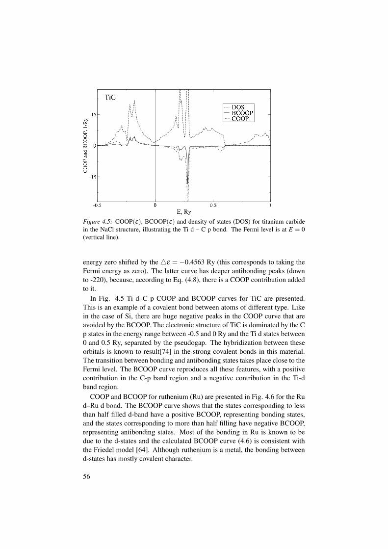
Figure 4.5: COOP(ε), BCOOP(ε) and density of states (DOS) for titanium carbidein the NaCl structure, illustrating the Ti d – C p bond. The Fermi level is at E = 0(vertical line).

energy zero shifted by the ε = −0.4563 Ry (this corresponds to taking theFermi energy as zero). The latter curve has deeper antibonding peaks (downto -220), because, according to Eq. (4.8), there is a COOP contribution addedto it.

In Fig. 4.5 Ti d–C p COOP and BCOOP curves for TiC are presented.This is an example of a covalent bond between atoms of different type. Likein the case of Si, there are huge negative peaks in the COOP curve that areavoided by the BCOOP. The electronic structure of TiC is dominated by the Cp states in the energy range between -0.5 and 0 Ry and the Ti d states between0 and 0.5 Ry, separated by the pseudogap. The hybridization between theseorbitals is known to result[74] in the strong covalent bonds in this material.The transition between bonding and antibonding states takes place close to theFermi level. The BCOOP curve reproduces all these features, with a positivecontribution in the C-p band region and a negative contribution in the Ti-dband region.

COOP and BCOOP for ruthenium (Ru) are presented in Fig. 4.6 for the Rud–Ru d bond. The BCOOP curve shows that the states corresponding to lessthan half filled d-band have a positive BCOOP, representing bonding states,and the states corresponding to more than half filling have negative BCOOP,representing antibonding states. Most of the bonding in Ru is known to bedue to the d-states and the calculated BCOOP curve (4.6) is consistent withthe Friedel model [64]. Although ruthenium is a metal, the bonding betweend-states has mostly covalent character.

56

Figure 4.6: COOP(ε), BCOOP(ε) and density of states (DOS) for hcp ruthenium,illustrating the Ru-Ru bond between two sublattices. The height of the COOP peak at+1 Ry is -660 1/Ry. The Fermi level is at E = 0 (vertical line).

Figure 4.7: BCOOP(ε) and the density of states (DOS) for bcc sodium (Na), illustrat-ing metallic bonding. The Fermi level is at E = 0 (vertical line).

57

Figure 4.8: BCOOP(ε) for the rock salt (NaCl), illustrating ionic bonding. The Fermilevel is at E = 0 (vertical line).

Our next two examples deal with other types of bonding, namely metal-lic and ionic. Only the BCOOP curves are presented. Bcc sodium (Na) isa system with nearly-free electrons and a pure metallic bonding. DOS andBCOOP curves for Na are presented in Fig. 4.7. The DOS curve has al-most free-electron (parabolic) shape. The total BCOOP curve is not unlikethe covalent-bonding curves presented above. The most profound differenceis that the total BCOOP for Na stays positive well above the Fermi level,while for the covalent-bonding systems there are clearly defined bonding andantibonding regions.

The rock salt (NaCl) is an insulator and a textbook example of the ionicbonding. The electronic structure of NaCl includes Cl 3s band at approxi-mately -0.9 Ry, Cl 3p band just below the Fermi level and the unfilled Na 3sband starting at +0.4 Ry. In the ideal case of purely ionic bonding the BCOOPwould be zero, since there is no hybridization in this limit. BCOOP is an in-dicator of the covalent bonding and it cannot measure the strength of the ionicbonding (the electrostatic Madelung energy). BCOOP of NaCl (Fig. 4.8) issmall in magnitude and negative up to the Fermi level. This is the small cova-lent contribution to the bond, which can be neglected compared to the strongionic bonding.

With these examples we have shown how BCOOP can distinguish betweendifferent types of chemical bonding. It also says which states give contributionto each covalent bond.

58

Figure 4.9: The crystal structure of Ti3SiC2 and Nb3SiC2 .

4.5 Nb3SiC2 – a theoretically predicted new MAX phaseNow it is time to apply BCOOP analysis to a more complicated systems. I amgoing to present the results for the Nb3SiC2 in this section (based on PaperIV) and for the MgB2 in the next section (based on Paper V).

Recently a new set of layered metallic ceramics have been discovered [75].They are called MAX phases because of their chemical composition Mn+1AXn,(n=1-3 have been reported) where M is an early transition metal, A is usuallya p-element and X is carbon or nitrogen. The nano-layered structure of MAXphases results in a combination of very interesting and useful properties, e.g.refractory ceramic properties, damage tolerance with the ability to withstandthermal shock, and also good electrical and tribological properties. The mostknown MAX phase is Ti3SiC2. Figure 4.9 shows its crystal structure. It canbe described as a layered structure consisting of TiC layers interleaved withSi monolayers. There are two nonequivalent positions of titanium: Ti(1) andTi(2).

In Paper IV we have investigated chemical stability of the MAX phaseNb3SiC2 from first principles theory. This phase has not been yet discoveredexperimentally. From the general trends in chemical bonding of transitionmetal carbides and silicides one would predict Nb3SiC2 to be significantlyharder than Ti3SiC2. Our total energy calculation have been done withinthe local density approximation. They demonstrate that Nb3SiC2 is unstable,

59

namely it would decompose into binary compounds as

Nb3SiC2 → 2NbC+27

NbSi2 +17

Nb5Si3. (4.20)

However, the energy gain from this reaction (formation energy of Nb3SiC2)is rather small, namely +0.02 eV/atom. Therefore we speculate that it mightexist as a metastable phase.

Our speculation is based on the comparison to the Ti-Si-C phases. TheMAX phases Ti3SiC2, Ti4SiC3, Ti5Si2C3 and Ti7Si2C5 have been recentlyobtained as thin films[76]. However, Ti5Si2C3 and Ti7Si2C5 are found tobe unstable from the DFT calculations, with the formation energies +0.04eV/atom and +0.03 eV/atom respectively. The latter phases are not observedin the bulk form, only as thin films. Since the formation energy per atom ofNb3SiC2 is even smaller than that of Ti5Si2C3 and Ti7Si2C5, it is likely thatthis compound can also be synthesized in thin film form.

The calculated bulk modulus for Nb3SiC2 is pretty high, 269 GPa (com-pared to the calculated value of 225 GPa for Ti3SiC2). Hence, our result isconsistent with the speculation that Nb-based MAX phases should be stifferthan the Ti-based ones.

In order to analyze the electronic structure and the chemical bonding weshow in Fig. 4.10a the density of states (DOS) of Nb3SiC2 and in Fig. 4.10bwe present the BCOOP for the Nb d – C p (Si p) bonds. The DOS of Nb3SiC2is fairly similar to that of Ti3SiC2 [76], except for the small gap betweenthe C 2s band and the valence band, and also the Fermi level being situatedhigher up in the band structure for Nb3SiC2. In both cases, the valence bandis dominated by the hybridizing M d – C p and M d – Si p states, which formcovalent bonds.

From Fig. 4.10b we observe that the BCOOP curves have well-definedbonding (positive) and antibonding (negative) regions with the crossover pointnear the Fermi level, which is a sign of predominantly covalent bonding char-acter. The states precisely at the Fermi level have mostly antibonding char-acter. From the BCOOP curves one can see that the Nb 4d – C 2p bonds arestronger than the Nb 4d – Si 2p ones. There is also a slight difference be-tween the Nb(1) 4d – C 2p and the Nb(2) 4d – C 2p bonds. The latter ones areweaker since they have a significant fraction of antibonding states below theFermi level. The Nb 4d – C 2p BCOOP curves are very similar to the Ti 3d –C 2p BCOOP curves in TiC (Paper III) and Ti3SiC2 [76], hence the bondingcharacter is also similar.

60

Figure 4.10: The partial DOS (a) and BCOOP (b) of Nb3SiC2 . The thin vertical lineshows the Fermi level ( E = 0). All BCOOP curves are normalized per one nearestneighbor bond.

Figure 4.11: The crystal structure of MgB2. The magnesium layer is displayed withgray circles and the boron layer is displayed with white circles.

61

-1 -0.5 0 0.5 1

Energy (Ry)

0

1

2

3

4

5

6

PDO

S (

stat

es· R

y -

1 )

B - sB - pB - d

0

1

2

3

4

Mg - sMg - pMg - d

Figure 4.12: The partial density of states (PDOS) of MgB2.

4.6 Chemical bonding in MgB2

In this section, which is based upon results of Paper V, we use BCOOP to an-alyze the chemical bonding in the famous superconductor MgB2 [77], whichhas a rather high critical temperature of 39 K. MgB2 has a layered crystalstructure which is shown in Fig. 4.11.

The chemical bonding in MgB2 is somewhat complicated. Previous studies[78, 79] suggest that the B—B in-plane bonding is of strong covalent char-acter, the Mg-–B inter-plane bonding has mainly ionic character, and the in-plane Mg-–Mg bonding is essentially metallic. This means that all three maintypes of chemical bonding coexist in MgB2, making it a tough test system forBCOOP.

We have calculated charge densities, PDOS and BCOOP for MgB2 usingthe FP-LMTO method within the generalized gradient approximation (GGA).The charge density plots (Figs. 4–6 of Paper V) clearly support the pictureoutlined above. One can see obvious covalent bonds between B atoms, but nocovalent bonds involving Mg atoms. Our calculation estimates that each Mgatom in MgB2 loses about 0.5 electron compared to the case of pure metallicmanganese. This charge transfer is a clear indication of ionic Mg–B bonding.

The partial density of states (PDOS) of MgB2 is presented in Fig. 4.12,while the BCOOP is shown in Fig. 4.13. The B–B BCOOP curves (Fig. 4.13,middle panel) show a positive region at lower energies and a negative region

62

-2-10123

BC

OO

P (s

tate

s·R

y-1) -1.5

-1

-0.5

0

-1 -0.5 0 0.5 1

Energy (Ry)

-1

-0.5

0

0.5

Mg(p) - B(p)Mg - B (total)

Mg(s) - B(s)Mg(s) - B(p)Mg(p) - B(s)

B(s) - B(s)B(s) - B(p)

B(p) - B(p)B - B (total)

Mg(p) - Mg(p)Mg - Mg (total)

Mg(s) - Mg(s)Mg(s) - Mg(p)

Figure 4.13: The BCOOP of MgB2. The upper, middle and lower panels show Mg–B,B–B and Mg–Mg BCOOP curves respectively.

at higher energies. This is a clear picture of covalent bonding, with bond-ing states (positive BCOOP) being separated from antibonding ones (negativeBCOOP). Our calculations reveal that the biggest contribution to the B–Bbonding comes from the p—p orbital overlap, while the s–s bond has someantibonding states below the Fermi level.

The upper panel of Fig. 4.13 shows the BCOOP between Mg and B. Thisis a more or less clear BCOOP picture of the ionic bonding (compare to ourNaCl example above). Remember that BCOOP is unable to describe ionicbonds adequately, and the ionic BCOOP curve is mostly negative both aboveand below the Fermi level.

Finally, the Mg–Mg BCOOP curves are presented in the lower panel ofFig. 4.13. They do not show as clear metallic picture as in our previousexample of Na (due to the much more complicated electronic structure ofMgB2), but at least there are no strong covalent bonds between Mg atoms,suggesting that the Mg–Mg bonding has predominantly metallic character. Tosummarize, BCOOP analysis is consistent with the previous studies of thechemical bonding in MgB2.

63

5 Hydrogen–hydrogen interaction andstructural stability of Ti3SnHx

Metal–hydrogen (M–H) systems are well-known for their numerous techno-logical applications, such as hydrogen storage[80, 81], fuel cells and nickel–hydrogen batteries. Many solids are able to absorb hydrogen in a certain pres-sure and temperature range. Hydrogenation can change literally any physicalproperty of the host material. It can cause a metal-insulator transition[82],change the material from ductile to brittle, or from paramagnetic to ferromag-netic etc. This can be used to tune the properties of certain materials, forexample Fe/VHx magnetic multilayers[83]. Since hydrogen atoms are small,they cannot substitute atoms of the host, instead they place themselves in theinterstitial, usually occupying tetrahedral or octahedral voids between largeratoms. Thus, an M–H system is a kind of an interstitial alloy. Due to the small-ness of the H atoms the volume change is minimal. Sometimes, however, thehost crystal structure changes upon hydrogenation.

Hydrogen storage and other applications require answers to the questions"How many H atoms can a metal take?" and "How close can the H atoms cometogether?" The answer for the first question is: the largest known H/M ratio(number of H atoms per metal atom) is 3.6 for thorium. The answer to thesecond question is the well-known "2 Å rule": the minimal H–H distance is2.1 Å. However, a few known exceptions such as Th2AlH4 [84], K2ReH9 [85]and RT InH4/3 (R = La, Ce, Pr, or Nd; T = Ni, Pd, or Pt) [86], require to putthis threshold down to about 1.8 Å. However, even this H–H distance is stilllarge compared to the one in the H2 molecule (0.74 Å). In other words, thereare no H2 molecules inside the metal host. In this chapter, which is based uponPapers VI and VII, we investigate how the M–H bonding leads to an effectiveH–H interaction in crystals. This interaction is responsible for the two limitsmentioned above. After the basics of the H–H interaction are given, we focuson the Ti3SnHx system. Upon hydrogenation, Ti3Sn undergoes a structuralphase transition, which, as shall be demonstrated, reflects the H–H interactionin a very clear way. We investigate this system using first-principles calcula-tions in order to learn the nature of the H–H interaction.

65

M

H

(a)M

(b)

Figure 5.1: (a) One H atom in the metal lattice: H–M interaction potential. (b) Twoatoms: H–H interaction comes into play.

5.1 Hydrogen-metal and hydrogen-hydrogen interactionsWhat is the metal-hydrogen interaction? What is the hydrogen-hydrogen in-teractions? Suppose we put a single hydrogen atom into the metal lattice(Fig. 5.1 a). The total energy of such a system depends on the position ofthe H atom: it has minima in the voids between M atoms, while it becomesextremely large close to the metal nuclei. We write the total energy as

E(R) = EM +EHM(R), (5.1)

where EM is the total energy of the host without hydrogen, and R is the H atomposition. The remaining contribution EHM(R) can be called hydrogen-metalinteraction potential. This is shown schematically in Fig. 5.1 a. Note thatif we put a hydrogen atom into a void, metal atoms actually shift outwards,and such structure relaxation somewhat lowers the total energy. Therefore,the hydrogen-metal interaction can be decomposed into electronic and elasticparts. To define the electronic part we assume that the structure relaxationdoes not occur, i.e. the metal atoms stay exactly where they were, and look atthe total energy. The remaining contribution to EHM comes from the structurerelaxation, hence it can be called elastic.

What happens if we put two H atoms into a metal? If two hydrogen atomsinteracted with the metal independently, the total energy would be

Enaive = EM +EHM(R1)+EHM(R2). (5.2)

In reality H atoms feel the presence of each other. The correct total energy is

E = EM +EHM(R1)+EHM(R2)+VHH(R1,R2), (5.3)

where the H–H pair potential VHH(R1,R2) is defined by Eq. 5.3, i.e. it is"everything beyond the independent H-atoms approximation" [64, 87] .

It can be rewritten as a function of R1 −R2 and (R1 + R2)/2. Why doesVHH depend on R1 −R2 and (R1 + R2)/2, and not just on the H–H distance|R1 −R2|? Because our H atoms are not placed in vacuum. The H–H inter-action in vacuum is well known: it is repulsive at short distances, attractive

66

Figure 5.2: Unit cell of Ti3SnH in (a) the D019 structure, (b) the E21 structure.

at larger distances, with the equilibrium point at dHH ≈ 0.74 Å, where the H2molecule is formed. Our VHH, however, is an effective interaction of the twoH atoms embedded into the metal, and it does depend on both R1 −R2 and(R1 +R2)/2.

What is the role of the H–H interaction? Independent H atoms would oc-cupy any suitable voids they found, and there are plenty of crystal structureswith voids located closer to each other that 2Å. However, a strong hydrogen-hydrogen repulsion or blocking exists at a range about 2Å, leading to the 2Årule. Can this effect be reproduced by any simple theoretical model? The jel-lium model (uniform electron gas with a positive background) might seem tobe a suitable model for a metal. However, two H atoms in jellium[88] form anH2 molecule with the H–H separation close to 0.74 Å for all electron densities,hence jellium is not an adequate model in this case.

H–H interaction can be decomposed into elastic and electronic contribu-tions, in the same way as the M–H interaction. The elastic H–H interactionis an extremely long range one, it can be both attractive and repulsive, de-pending on the material and strain[89]. In this chapter we focus mainly on theelectronic H–H interaction, since, as it will be shown below, it is the one thatis mainly responsible for blocking and structural phase transitions.

5.2 Ti3SnHx as a model systemThe H–H repulsion makes it energetically favorable to maximize H–H dis-tances. Therefore many metallic systems undergo a structural phase transitionupon hydrogenation. As a result, a new crystalline hydride phase is formedwith a structure different from that of the initial metal host. An example ofsuch system is Ti3Sn, and we have chosen it to study the H–H interaction forthe reasons described below. Ti3Sn has a hexagonal D019 structure (Fig. 5.2a).When we start do put hydrogen into Ti3Sn [90, 91], at first the structure doesnot change. Ti3SnHx exists in the hexagonal D019 structure for x < 0.7 as an

67

Figure 5.3: Heat of formation of Ti3SnHx versus volume. ∆E ≡ E(Ti3SnHx)−x2 E(H2)− Ehex(Ti3Sn)|V=Veq

. Squares and circles denote cubic and hexagonal phaserespectively. Empty, striped and filled symbols denote x = 0,0.5 and 1 respectively.

interstitial solution, with H atoms occupying the Ti6 octahedral voids. Uponfurther hydrogenation the Ti3SnH hydride phase is formed. Ti3SnH crystal-lizes in the cubic E21 structure (Fig. 5.2b), with H atoms still occupying theTi6 octahedral voids.

These two crystal structures are very similar despite completely differentsymmetries (D019 is hexagonal while E21 is cubic). The situation is similarto the fcc and hcp structures of transition metals1. They have different sym-metry, but almost identical nearest neighbor geometry. The biggest differencebetween the D019 and E21 structures is the H–H distance, which is quite large(≈ 4.18 Å) in the cubic phase and small (≈ 2.3 Å) in the hexagonal one (close,in fact, to the 2 Å limit). The Ti6 octahedral voids form a cubic sublattice inthe cubic phase, but they form a set of parallel chains in the hexagonal phase(Fig. 5.2). One can look at the phase transition as a way for the system todecrease its energy by increasing H–H distances. Since the two structures areotherwise very similar, the structural phase transition can be attributed to theH–H repulsion alone. This fact makes Ti3SnHx a good choice to study theH–H interaction.

We have investigated the structural stability of Ti3SnHx using the VASPplane wave code[68] with PAW potentials [67, 68]; within the LDA approx-

1Under certain experimental conditions a third, orthorhombic form of Ti3SnHx is formed. Thelatter structure is discussed in details in Paper VII.

68

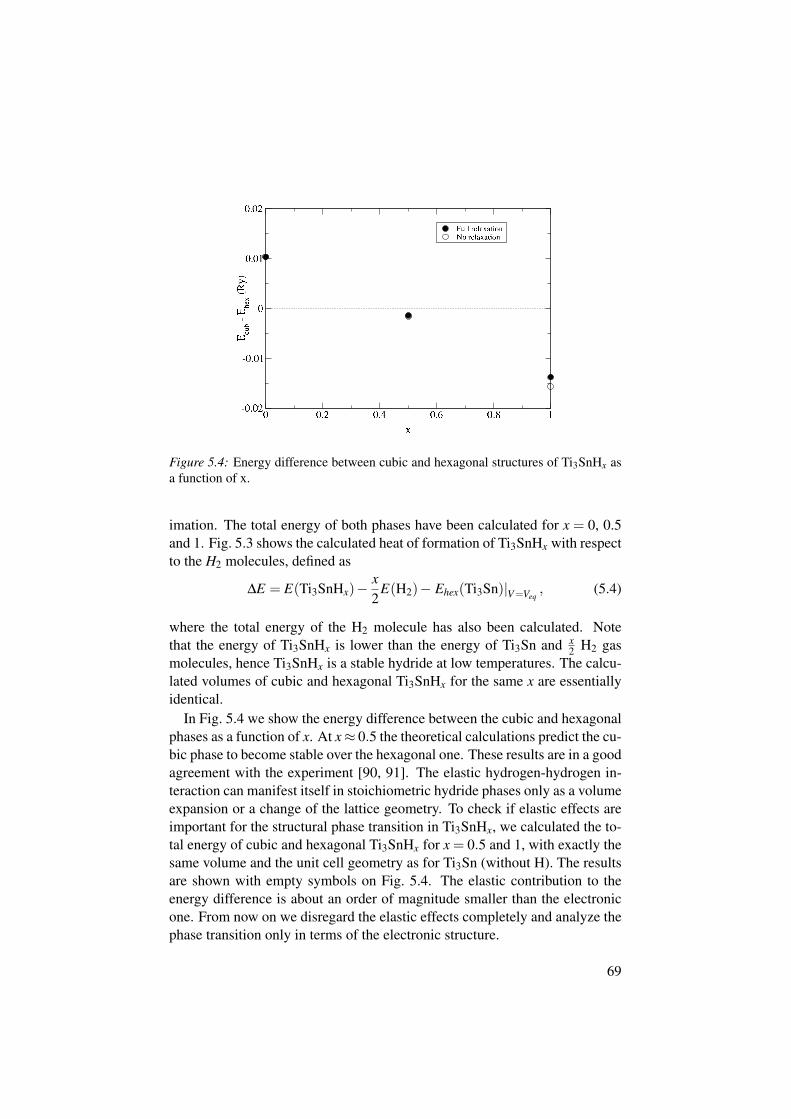
Figure 5.4: Energy difference between cubic and hexagonal structures of Ti3SnHx asa function of x.

imation. The total energy of both phases have been calculated for x = 0, 0.5and 1. Fig. 5.3 shows the calculated heat of formation of Ti3SnHx with respectto the H2 molecules, defined as

∆E = E(Ti3SnHx)− x2

E(H2)− Ehex(Ti3Sn)|V=Veq, (5.4)

where the total energy of the H2 molecule has also been calculated. Notethat the energy of Ti3SnHx is lower than the energy of Ti3Sn and x

2 H2 gasmolecules, hence Ti3SnHx is a stable hydride at low temperatures. The calcu-lated volumes of cubic and hexagonal Ti3SnHx for the same x are essentiallyidentical.

In Fig. 5.4 we show the energy difference between the cubic and hexagonalphases as a function of x. At x≈ 0.5 the theoretical calculations predict the cu-bic phase to become stable over the hexagonal one. These results are in a goodagreement with the experiment [90, 91]. The elastic hydrogen-hydrogen in-teraction can manifest itself in stoichiometric hydride phases only as a volumeexpansion or a change of the lattice geometry. To check if elastic effects areimportant for the structural phase transition in Ti3SnHx, we calculated the to-tal energy of cubic and hexagonal Ti3SnHx for x = 0.5 and 1, with exactly thesame volume and the unit cell geometry as for Ti3Sn (without H). The resultsare shown with empty symbols on Fig. 5.4. The elastic contribution to theenergy difference is about an order of magnitude smaller than the electronicone. From now on we disregard the elastic effects completely and analyze thephase transition only in terms of the electronic structure.

69

Ti

H

x

x

(a)

Ti

H

(b)

2x

Ti

H

x

x

(c)

Figure 5.5: Geometrical configurations of two hydrogen atoms displaced along the[011] direction. The unit cell is shown for the following configurations: (a) reference(b) hydrogen atoms centered on a Ti6 octahedron (1b site) and (c) hydrogen atomscentered on a Ti4Sn2 octahedron (3d site). The crystal structure is cubic and shownfor a cut spanned by the vectors [001] and [010]. The small black dot shows the Ti6site.

5.3 The H–H pair potential

In this section we analyze the structural phase transition in Ti3SnHx in termsof the H–H interaction potential introduced above. In the spirit of Eq. (5.3),the total energy of this system can be written as

E = EM +∑i

EHM(Ri)+12 ∑

i jVHH(Ri,R j). (5.5)

Here we ignore the triple and higher order interactions of the hydrogen atoms.Note that the host energy EM depends on the electron density, and thus im-plicitly on the hydrogen concentration. Can the observed phase transition bemerely a band-filling effect? Our virtual crystal approximation (VCA) calcula-tion demonstrate that the difference Ecub−Ehex for Ti3Sn is almost insensitiveto the band filling. Hence the structural phase transition is caused by the sec-ond and third terms in Eq. (5.5). Since the nearest neighbor distances coincidefor the two phases of Ti3SnHx, the nearest neighbor terms in ∑i EHM(Ri) donot contribute to Ecub−Ehex, and the third term in Eq. (5.5) is expected to givethe main contribution to the x-dependence of Ecub −Ehex.

70

Our next step is to calculate the hydrogen-hydrogen pair potential from thefirst principles. We use supercells with displaced H atoms in the rigid Ti3Snmatrix. The supercells have to be chosen carefully, our choice is presentedin Fig. 5.5. In all three cases the unit cell of cubic Ti3SnH is doubled alongthe z-direction to include two formula units, hence the supercell is small. TheH atoms are displaced along the [110] direction, along the line connectingdifferent octahedral voids, and there are no metal atoms in between. The Hatoms can move away from each other up to

√2a ≈ 5.9 Å.

In order to exclude the hydrogen–metal interaction we use the supercellwhich we call the reference configuration (Fig. 5.5a). It keeps the H–H dis-tance constant and equal to the lattice constant a = 4.2 Å. The other two con-figurations have the H–H distances varied, with the pair of H atoms centeredat the 1b site (Fig. 5.5b) or at the 3d site (Fig. 5.5c). From now on we neglectthe H–H interactions at distances larger than or equal to a. This means that theenergy of the reference configuration is given by the H–M interaction alone

Eref = EM +EHM(R1)+EHM(R2), (5.6)

where R1,2 are the positions of the hydrogen atoms and the energy is definedper supercell (two formula units). For the configurations of Fig. 5.5(b,c) theH–H interaction within the pair should be also taken into account

E = EM +EHM(R1)+EHM(R2)+VHH(d), (5.7)

where d is the H–H distance and it is equal to 2x and√

2a− 2x for the con-figurations of Fig. 5.5b and c, respectively, where x is the displacement of theH atom from the 1b site. The H–H pair potential can now be calculated fromEqs. (5.7) and (5.6) as

VHH(d) = E(x)−Eref(x). (5.8)

The total energy as a function of x for our three configurations is presentedin Fig. 5.6a. The reference curve is basically the plot of the H–M potential. Ithas the global minimum at x = 0, which means that H atoms sit at the 1b (Ti6)sites, which gives the cubic Ti3SnH phase. It also has the local minimum at 3d(Ti4Sn2) sites and a potential barrier in between. The other two curves havehigher total energy than the reference one. Both curves have a local minimumcorresponding to a molecular hydrogen-like state at the respective octahedralvoid, with d = 0.9 Å and 1 Å for 1b and 3d sites respectively. This is a bitlarger than the d = 0.7 Å for the free H2 molecule. Note that these distancesminimize the total energy, which includes both H–H and H–M interactions.

The calculated VHH(d) curves are presented in Fig. 5.6b. The 1b and 3dcurves are not exactly the same which means that the pair potential is indeeda function of not only R1 −R2, but also of (R1 +R2)/2. However, both pair

71

Figure 5.6: (a) Total energy for the three H configurations along the [011] direction asfunction of the displacement x from the 1b site. (b) H–H pair potentials in the [011]direction.

72

potentials have the same general structure. At short range there is strong re-pulsion between the H atoms, similar to that of an H2 molecule. For largerdistances the attraction caused by the covalent H–H bonding dominates. Theminimum of the H–H pair potential is reached at about 1.6 and 1.2 Å for the 1band 3d configurations, respectively. The pair potential curves at Fig. 5.6b canbe viewed as a superposition of the ’normal’ contribution (e.g. as calculatedin a jellium host [88]), and a long-range repulsive component. The ’normal’contribution alone would result in a bond distance of about 0.7 Å. The originof the repulsive component will be discussed below.

Let us apply the pair potential model to the structural phase transition inTi3SnHx. Although our VHH(d) curves were calculated for specific cubic su-percells of Fig. 5.5, we assume for the moment that these potentials havethe general character and can be also applied to the hexagonal Ti3SnHx. Weonly take into account the strongest interaction, namely the interaction of anH atom in hexagonal Ti3Sn with its two H neighbors within the chain

(Ecub −Ehex)Ti3SnH = (Ecub −Ehex)Ti3Sn −VHH(d). (5.9)

With d = 2.3 Å (the H–H distance in the hexagonal Ti3SnH phase), the ob-tained estimates of (Ecub−Ehex)Ti3SnH− (Ecub−Ehex)Ti3Sn are -21 mRy and -9mRy for the 1b and 3d curves respectively. As we remember, the total energycalculation gives the value of (Ecub −Ehex)Ti3SnH − (Ecub −Ehex)Ti3Sn = −24mRy. Thus, the 1b pair potential gives basically a quantitative agreement withthe direct DFT calculations, while the 3d one works much worse. This is nota surprise, since the H atoms in both cubic and hexagonal Ti3SnH have onlyTi nearest neighbors, while the 3d site has both Ti and Sn nearest neighbors.

5.4 Physics behind the H–H repulsionTo find the physics behind the H–H repulsion, we should take a look at theelectronic structure of Ti3SnHx. The calculated density of states (DOS) andpartial density of states (PDOS) of the cubic and hexagonal phases of Ti3SnHx

(x = 0 and 1) are presented in Fig. 5.7. The main change in DOS upon hydro-genation is the formation of a localized H s-like band about 0.5 Ry below theFermi level, between the valence band and the Sn s-like band (≈ −0.7 Ry).From the PDOS curve one can make conclusions about the character of thechemical bonding. In a purely metallic picture hydrogen would donate oneelectron into the rigid valence band of Ti3Sn. In a purely ionic picture thelocalized band of the H− ion with a pure H s character would be formed. And,finally, covalent bonding manifests itself in a strong hybridization betweenmetal and hydrogen. In our PDOS curves the localized H-induced band at 0.5Ry below EF has less than 50% H s character, with the rest coming from the

73

Figure 5.7: Partial density of states of (a) cubic Ti3Sn, (b) cubic Ti3SnH, (c) hexagonalTi3Sn, (d) hexagonal Ti3SnH.

74

Figure 5.8: Partial density of states of cubic Ti3SnH and Ti3Sn(H2)0.5. Solid curve –total DOS, dashed – H 1s, dotted – Ti 3d.

metal states, mainly Ti d states. This indicates a strong covalent bonding be-tween H atoms and their Ti nearest neighbors. As a result, Ti 3d states, whichin Ti3Sn are occupied in the region between -0.4 Ry and the Fermi level, canin the hydrogenated phase lower their energy substantially since they occupystates down to -0.6 Ry. From the PDOS curves we conclude that Ti3SnH is astable hydride due to the strong Ti–H covalent bonding.

To understand the microscopic nature of the H–H interaction, we mustknow how the electronic structure of Ti3SnHx depends on the H–H distance.In order to do that, we build a superstructure with an H2 molecule immersedinto the Ti6 octahedron, and call it Ti3Sn(H2)0.5 structure. The structure isquite similar to that of Fig. 5.5 b, but this time we align the H atoms alongthe [001] direction, purely for the purpose of convenience. We compare inFig. 5.8 the DOS and PDOS of the cubic Ti3SnH and of the Ti3Sn(H2)0.5structure (with H–H distance d = 0.66 Å). As one can see from Fig. 5.8, themain difference between the two PDOS curves is the position and characterof the localized H s-like band. For cubic Ti3SnH, it is a strongly hybridizedband about 0.5 Ry below the Fermi level. For Ti3Sn(H2)0.5, however, the H

75

1s states are situated below the Sn s band and the hybridization with all otherstates in the crystal is weak. The feature at 0.9 Ry below E f can be viewed asthe bonding state of a H2 molecule immersed in Ti3Sn. This molecule is onlyweakly influenced by the surrounding Ti and Sn atoms. The hybridizationbetween metal and hydrogen states is weak for Ti3Sn(H2)0.5.

The reason for the H–H repulsion in Ti3SnHx seems to be the competitionbetween the H–H and the M–H covalent bonding. When the H atoms arefar apart, there is a strong M–H covalent bonding. When they move closer,the H–H covalent bonding appears, which, by itself would favor short H–H distance. However, this H–H bonding weakens the stronger M–H bonds,increasing the total energy. Finally, the H2 molecule in the metallic host isenergetically unfavorable (although it may correspond to a local minimum ofthe total energy). This mechanism leads to the H–H repulsion for the H–Hdistances larger than approximately 2Å, and hence to the "2Å rule".

76

6 Sammanfattning på svenska

Teoretiska studier i tvådimensionell magnetism och kemisk bindning

Denna avhandling inkluderar flera fysiskproblem. För att lösa dessa prob-lem behöver man både lite teoretiskt arbete och datorberäkningar. Teoretisktarbete handlar om att formulera ekvationer och det kan göras bara med papperoch penna. Syftet med teoretisk fysik är att utveckla teoretiska formalismersamt även att formulera nya teorier. Beräkningsfysik använder teorier och ek-vationer som redan finns (som är redan utvecklade inom teoretisk fysik) ochtillämpar dom på realistiska system, ofta med hjälp av moderna datorer. Ar-betet i denna avhandling ligger någonstans mellan teoretisk fysik och beräkn-ingsfysik. Vi har utfört numeriska beräkningar men även utvecklat teoretiskamodeller när det behövdes.

Denna avhandling består av två delar. I den första delen studerar vi ter-modynamik av en tvådimensionell Heisenberg ferromagnet med dipolär väx-elverkan. Det är den mest teoretiska delen av avhandlingen. Låt oss härförsöka förklara den komplicerade titeln på projektet. Vad är en tvådimen-sionell Heisenberg ferromagnet? Tvådimensionella (2D) magneter är mag-neter i form av tunna folier eller multilager. En ferromagnet är en typ avmagnet som kan vara magnetiserad även utan ett externt magnetiskt fält. Met-aller som järn, kobolt och nickel är exempel på ferromagneter. Själva ordet"ferromagnet" kommer faktisk från "ferrum", det latinska ord för järn.

Tvådimensionella magnetiska system har extremt viktiga tekniska tillämp-ningar. Nämligen, tvådimensionella magneter används för magnetisk data-lagring. I hårddiskar används tvådimensionella magnetiska material bådeför hårddisken (lagringsmedia) och för avläsning- samt inspelningshuvudet.Magnetiska multilager används också i magnetiska sensorer, små perma-nenta magneter, spintronikenheter etc. Heisenbergmodellen är en populärteoretisk modell som beskriver magnetismen hos ett magnetiskt material.Denna modell fungerar för magneter med väldig lokalizerade magnetiskamoment. I Heisenbergmodellen introducerar man spinnoperatorer (kvant-Heisenbergmodellen) eller spinnvektorer (klassisk Heisenbergmodell) som ärpositionerade på noder i ett kristallgitter. Varje spinnoperator eller spinnvek-tor representerar ett lokalt magnetisk moment som ligger på en gitternod (enmagnetisk atom). Ferromagnetens magnetiska egenskaper beror bl.a. på tem-peratur. Om man värmer en magnet kommer de magnetiska momenten att

77

minska, tills dess att vid en temperatur som kallas för Curietemperatur (Tc)försvinner alla tecken på magnetisk ordning. Det är denna "termodynamik"som vi har studerat med en Heisenbergmodell. Vi har undersökt hur mag-netiseringen beror av temperatur och vi vill även veta Curietemperaturen påalla magnetiska material vi studerar. För praktiska tillämningar vill man ha såstort Tc som möjligt, åtminstone mycket högre än rumtemperatur. I vissa fall,t.ex. för elmotorer, krävs en ännu högre temperatur för att man kan användadet magnetiska materialet i tillämpningar.

Dipolväxelverkan är den "magiska" växelverkan mellan två magneter viadet magnetfält som alla barn känner till (t.ex. när man undersöker två kyl-skåpsmagneter). Två magneter kan känna av varandra på ett asvstånd avnågra centimeter. Därför säger man att dipolväxelverkan har en lång räck-vidd. Egentligen är denna kraft också viktigt för den mikroskopiska struk-turen av det magnetiska materialet. I tredimensionella (vanliga) magneterresulterar dipolväxelverkan i så kallad domänstruktur. Domänstruktur bety-der att smådelar av en magnetisk kristall (domäner) är magnetiserade i olikariktningar, så att den totala magnetiseringen för materialet är lika med noll.Domänstrukturen bildas eftersom den låter en magnetisk kropp minska dessdipolära energi, och det är det som är orsaken till att dom flesta järn- ochstålsaker inte verkar vara magnetiserade. I tvådimensionell magnetism spelardipolväxelverkan en helt annan roll. Mermin-Wagners teorem påstår att en"ideal" tvådimensionell magnet skulle inte ha någon magnetiskt ordning alls,inte vid någon temperatur förutom precis vid den absoluta nollpunkten (0grader Kelvin). Detta fenomen inträffar eftersom vid en ändlig temperaturblir Heisenbergmodellen exciterad. De viktigaste excitationerna i Heisen-bergmodellen är magnoner, kvanta av spinnvågor. Spinnvågor går genom enmagnet ungefär som ljud går genom luften och de förstör den magnetiskaordningen i tvådimensionella magneter. I verkligheten existerar 2D magneterutan problem vid ändlig temperatur, trots att de oftast har lägre Curietemper-atur än vanliga (tredimensionella) magneter. En av orsakerna till detta är justdipolväxelverkan som bryter det strikta krav som ställs av Mermin-Wagnersteorem.

I denna avhandling har vi behandlat både klassiska spinn och kvantspinn.För att studera den två-dimensionella Heisenbergmodellen har vi modifieraten teori som heter självkonsistent spinnvågsteori (SSWT) för att inkluderaden dipolära växelverkan. Denna teori beskriver magnetens termodynamikgenom att introducera magnoner och betraktar magon–magnon växelverkanpå ett visst enkelt sätt. Temperatur-renormalisering av dipolväxelverkan medkvadraten av magnetiseringen behövs också för att bygga en fungerande formav självkonsistent spinnvågsteori. Våra resultat är att Curietemperaturen berorpå spinnvärde (i kvantfall) samt på styrkan hos dipolväxelverkan. För klas-siska spinn ligger våra resultat inom 9% från exakta beräkningar med nu-

78

meriskt utmanande Monte Carlo simuleringar. Våra resultat är mycket bät-tre än "vanlig" spinnvågteori (som behandlar magnoner utan magon–magnonväxelverkan) och Tyablikov-approximationen. Ett annat markvärdigt resul-tat är att för tvådimensionella magneter är det viktigt att använda kvantspinnoch inte klassiska spinn. Även stora spinn som t. ex. S = 7/2 är inte riktigt"klassiska" utan uppvisar kvantegenskaper. För tredimensionella magneterfungerar en klassiskt behadling av spinnen ofta ganska bra. Fördelen med vårteori är att den lätt kan behandla kvantspinn, emedan andra teorier, som t. ex.Monte Carlo metoden, har mycket svårara att göra detta.

I den andra delen av avhandlingen har vi studerat kemisk bindning i fastakroppar med hjälp av elektronstrukturberäkningar. Kemisk bindning är denkraft som håller ihop alla molekyler samt fasta kroppar. Den kommer ur-sprungligen från Coulombattraktionen mellan de elektroner och kärnor sombygger upp materialet, men den kan ta många olika former i fasta kroppar(kovalent bindning, metallisk bindning, jonisk bindning etc.). Elektronstruk-turberäkningar baseras på täthetsfunktionalteori (DFT). Vad är nu detta förnågonting?

Kvantmekaniken beskriver alla kvantsystem, som t. ex. molekyler ellerfasta kroppar, med Schrödingerekvationen (eller den relativistiska Diracekva-tionen). Den använder vågfunktionen som beror på koordinater av alla elek-troner i systemet. Men en typisk kristall kan ha så många som 1023 elektroner.Man kan aldrig lösa Schrödingerekvationen för så många variabler i prak-tiken. Täthetsfunktionalsteorin kommer till hjälp då. Istället för att användavågfunktionen, så använder denna teori elektrontätheten som beror bara på trekoordinater. DFT var utvecklat på 1960-talet av Hohenberg, Kohn och Sham,och Walter Kohn fick Nobelprizet i 1998 i kemi för detta arbete.

När man utför DFT-beräkningar är målet ofta att veta vilken typ av kemiskbindning materialet har, och vilka atomer deltar i t.ex. kovalenta bindningar(kovalent bindning är när två atomer delar två elektroner och en "elektron-pinne" skapas mellan dem). De finns så kallade indikatorer för kemiskbindning som låter oss analysera den kemiska bidningen från elektronstruk-turberäkningar. I den här delen av avhandligen har vi utvecklat en ny kemisk"bindningsindikator" som vi kallat den balancerade kristallorbital överlapppopulationen (BKOOP på svenska och BCOOP på engelska). Vår metod ären utveckling av en tidigare indikator, och vi visar att vår metod är lämpli-gare för praktiska DFT beräkningar. Vi har tillämpat den nya indikatorn tillvissa, ur materialvetenskaplig synpunkt, intressanta system, som t.ex. densupraledande MgB2 föreningen och ett nytt keramiskt material, Nb3SiC2.MgB2 blir en supraledare med en kritisk temperatur Tc = 39K, som är hö-gre än Tc-n för nästan alla material (förutom hög-Tc kuprater). Detta mate-rial är också ett unikt ämne eftersom det består av element med tre typer avkemisk bindning (metallisk, jonisk och kovalent). Nb3SiC2 tillhör en familj av

79

s.k. MAX-faser, metalliska keramiker med nano-laminat struktur och kemiskformel Mn+1AXn. Vi förutspår att Nb3SiC2, om det skulle lyckas syntetiseras,kommer att vara marginellt metastabillt, och man kan förvänta sig att dennafas kan existera i tunna filmer.

I ett annat projekt har vi studerat väte–väte (H–H) växelverkan i metaller,som t. ex. i Ti3Sn. Detta problem är viktigt för väteförvaring. Vi visaratt H–H växelverkan orsakas av en tävling mellan väte–metall och väte–vätebindning. När tillräkligt mycket väte går in i Ti3Sn, byter materialet kristall-struktur, en effekt som vi kan förklara både med en enkel modell samt viaDFT beräkningar.

80

Acknowledgments

First I would like to thank my supervisor Olle Eriksson. This work would notbe possible without his inexhaustible energy, original ideas and a lot of prac-tical help. I am grateful to my other supervisors, Rajeev Ahuja and MikhailKatsnelson, for helping me learn how to be a physicist. Thank you, BörjeJohansson, for creating a unique "FYSIK4 atmosphere", which is still alivedespite us being several groups now. I thank Lars Nordström, Susanne Mirbt,Igor Abrikosov and Peter Oppeneer for making our groups function.

I thank John Wills for creating the FP-LMTO code and for helping me tohack it. My gratitude to all my collaborators and people I have discussedscience with: Marie Vennström, Yvonne Andersson, Valentin Irkhin, HelmutRathgen, Petros Souvatzis, Per Andersson, Sebastien Lebegue, Sam Shall-cross, Liviu "Lulu" Chioncel, Kay Dewhurst, Sangeeta Sharma, Anna Delin,and many others. My big thanks to Anders E., Per, Weine, Lars., Urban, Erik,Mamo, Adi, Björn, Thomas, Peter and Carlos for taking care of our computersystem.

Last, but not least, my deepest thanks to my family, and for all my friends,cofee- and beermates. That includes the people I met in Sweden: Weine, Lars,Velimir, Arkady, Sam, Sangeeta, Kay, Bengt, Thomas & Katrin & Alex, Hel-mut, Till, Ola, Petros, Björn, Jorge, Natasha "Apollonia" P., Seb, . . . ; and alsopeople I met elsewhere, Igor, Stas, Nick, Vasiliy, Andrey B., Alexei Soroka"AA" & Alexei Soroka "AK", Vera, Oksana K., Jaroslaw, Denis "Syoma"Semagin, Andrey S., Maria C., among others. I would not survive in a foreigncountry without your company.

81

References

[1] B. Heinrich and J. A. C. Bland, eds., Ultrathin Magnetic Structures I-II(Springer-Verlag, Berlin, 1994).

[2] S. A. Wolf, D. D. Awschalom, R. A. Buhrman, J. M. Daughton, S. vonMolnár, M. L. Roukes, A. Y. Chtchelkanova, and D. M. Treger, Science294, 1488 (2001).

[3] A. Taga, L. Nordström, P. James, B. Johansson, and O. Eriksson, Nature406, 280 (2000).

[4] P. Grünberg, R. Schreiber, Y. Pang, M. B. Brodsky, and H. Sowers, Phys.Rev. Lett. 57, 2442 (1986).

[5] M. N. Baibich, J. M. Broto, A. Fert, F. Nguyen Van Dau, F. Petroff,P. Eitenne, G. Creuzet, A. Friederich, and J. Chazelas, Phys. Rev. Lett.61, 2472 (1988).

[6] N. Mermin and H. Wagner, Phys. Rev. Lett. 17, 1133 (1966).

[7] H. Benson and D. L. Mills, Phys. Rev. 178, 839 (1969).

[8] R. P. Erickson and D. L. Mills, Phys. Rev. B 43, 10715 (1991).

[9] D. P. Pappas, K.-P. Kämper, and H. Hopster, Phys. Rev. Lett. 64, 3179(1990).

[10] V. L. Pokrovskii and M. V. Feigelman, Zh. Eksp. Teor. Fiz. 72, 557(1977), [Sov. Phys. JETP 45, 291 (1977)].

[11] S. T. Chui, Phys. Rev. B 50, 12559 (1994).

[12] J. Sasaki and F. Matsubara, J. Phys. Soc. Jpn. 66, 2138 (1997).

[13] A. B. MacIsaac, Physica A 239, 147 (1997).

[14] A. B. MacIsaac, J. P. Whitehead, M. C. Robinson, and K. De’Bell, Phys.Rev. B 51, 16033 (1995).

[15] A. B. MacIsaac, K. De’Bell, and J. P. Whitehead, Phys. Rev. Lett. 80,616 (1998).

83

[16] K. De’Bell, A. B. MacIsaac, and J. P. Whitehead, Rev. Mod. Phys. 72,225 (2000).

[17] O. Iglesias and A. Labarta, J. Magn. Magn. Mater. 221, 149 (2000).

[18] A. P. Levanyuk and N. Garcia, Journal of Physics: Condensed Matter 4,10277 (1992).

[19] A. Hucht, A. Moschel, and K. D. Usadel, J. Magn. Magn. Mater. 148,32 (1995).

[20] S. V. Maleev, Zh. Eksp. Teor. Fiz. 70, 2374 (1976), [Sov. Phys. – JETP43, 1240 (1976)].

[21] Y. Yafet, J. Kwo, and E. M. Gyorgy, Phys. Rev. B 33, 6519 (1986).

[22] P. Bruno, Phys. Rev. B 43, 6015 (1991).

[23] L. Hu, H. Li, and R. Tao, Phys. Rev. B 60, 10222 (1999).

[24] P. Fröbrich, P. J. Jensen, P. J. Kuntz, and A. Ecker, Eur. Phys. J. B 18,579 (2000).

[25] K. Yosida, Theory of Magnetism (Springer, Berlin, 1996).

[26] P. Mohn, Magnetism in the Solid State (Springer-Verlag, 2002).

[27] M. S. Makivic and H.-Q. Ding, Phys. Rev. B 43, 3562 (1991).

[28] J.-K. Kim, D. P. Landau, and M. Troyer, Phys. Rev. Lett. 79, 1583(1997).

[29] A. Cuccoli, T. Roscilde, V. Tognetti, R. Vaia, and P. Verrucchi, Phys.Rev. B 67, 104414 (2003).

[30] P. Henelius, P. Fröbrich, P. J. Kuntz, C. Timm, and P. J. Jensen, Phys.Rev. B 66, 094407 (2002).

[31] A. Cuccoli, V. Tognetti, R. Vaia, and P. Verrucchi, Phys. Rev. B 56,14456 (1997).

[32] A. Cuccoli, T. Roscilde, V. Tognetti, R. Vaia, and P. Verrucchi, Eur. Phys.J. B 20, 55 (2001).

[33] M. Takahashi, Prog. Theor. Phys. Suppl. 87, 233 (1986).

[34] M. Takahashi, Phys. Rev. Lett. 58, 168 (1987).

[35] M. Takahashi, Phys. Rev. B 36, 3791 (1987).

84

[36] D. P. Arovas and A. Auerbach, Phys. Rev. B 38, 316 (1988).

[37] V. Y. Irkhin, A. A. Katanin, and M. I. Katsnelson, Phys. Lett. A 157, 295(1991).

[38] V. Y. Irkhin, A. A. Katanin, and M. I. Katsnelson, Phys. Rev. B 60, 1082(1999).

[39] V. Y. Irkhin and A. A. Katanin, Phys. Rev. B 55, 12318 (1997).

[40] R. J. Birgeneau, H. J. Guggenheim, and G. Shirane, Phys. Rev. B 8, 304(1973).

[41] S. Tyablikov, Methods in the Quantum Theory of Magnetism (Plenum,New York, 1967).

[42] H. B. Callen, Phys. Rev. 130, 890 (1963).

[43] F. Bloch, Z. Phys. 61, 206 (1930).

[44] P. Fröbrich, P. J. Kuntz, and M. Saber, Ann. Phys. (Leipzig) 11, 387(2002).

[45] P. Fulde, Electron Correlations in Molecules and Solids (Springer,Berlin, 1995).

[46] P. Hohenberg and W. Kohn, Phys. Rev. 136, B864 (1964).

[47] W. Kohn and L. Sham, Phys. Rev. 140, A1133 (1965).

[48] L. Hedin and B. I. Lundqvist, J. Phys. C: Solid State Phys. 4, 2064(1971).

[49] U. von Barth and L. Hedin, J. Phys. C: Solid State Phys. 5, 1629 (1972).

[50] D. M. Ceperley and B. J. Alder, Phys. Rev. Lett. 45, 566 (1981).

[51] J. P. Perdew and A. Zunger, Phys. Rev. B 23, 5048 (1981).

[52] A. Görling and M. Levy, Phys. Rev. A 50, 196 (1994).

[53] A. Görling, Phys. Rev. B 53, 7024 (1996).

[54] M. Methfessel and A. T. Paxton, Phys. Rev. B 40, 3616 (1989).

[55] O. Jepsen and O. Andersen, Solid State Commun. 9, 1763 (1971).

[56] P. E. Blöchl, O. Jepsen, and O. K. Andersen, Phys. Rev. B 49, 16223(1994).

85

[57] O. K. Andersen, Phys. Rev. B 12, 3060 (1975).

[58] H. L. Skriver, The LMTO method: muffin-tin orbitals and electronicstructure (Springer, Berlin, 1984).

[59] J. M. Wills, O. Eriksson, M. Alouani, and D. L. Price, in Electronicstructure and physical properties of solids: the uses of the LMTO method(Springer, 2000), pp. 148–67.

[60] J. Trygg, Ph.D. thesis, Uppsala University (1995).

[61] J. C. Phillips and L. Kleinman, Phys. Rev. 116, 287 (1959).

[62] W. A. Harrison, Pseudopotentials in the Theory of Metals (W.A. Ben-jamin Inc., New York, 1966).

[63] N. W. Ashcroft, Phys. Lett. 23, 48 (1966).

[64] D. Pettifor, Bonding and Structure of Molecules and Solids (ClarendonPress, Oxford, 1995).

[65] D. R. Hamann, M. Schlüter, and C. Chiang, Phys. Rev. Lett. 43, 1494(1979).

[66] D. Vanderbilt, Phys. Rev. B 41, 7892 (1985).

[67] P. Blöchl, Phys. Rev. B 50, 17953 (1994).

[68] G. Kresse and D. Joubert, Phys. Rev. B 59, 1758 (1999).

[69] G. D. Mahan, ed., Many-Particle Physics (Plenum Press, New York andLondon, 1993).

[70] M. I. Katsnelson and A. I. Lichtenstein, J. Phys.: Condens. Matter 11,1037 (1999).

[71] T. Hughbanks and R. Hoffmann, J. Am. Chem. Soc. 105, 3528 (1983).

[72] R. Dronsowski and P. Blöchl, J. Phys. Chem. 97, 8617 (1993).

[73] N. Börnsen, B. Meyer, O. Grotheer, and M. Fähnle, J. Phys.: Condens.Matter 11, L287 (1999).

[74] C. D. Gelatt, A. R. Williams, and V. L. Moruzzi, Phys. Rev. B 27, 2005(1983).

[75] M. W. Barsoum, Prog. Solid St. Chem. 28, 201 (2000).

86

[76] J.-P. Palmquist, S. Li, P. O. Å. Persson, J. Emmerlich, O. Wilhelmsson,H. Högberg, M. I. Katsnelson, B. Johansson, R. Ahuja, O. Eriksson,et al., Phys. Rev. B 70, 165401 (2004).

[77] J. Nagamatsu, N. Nakagawa, T. Muranaka, and Y. Zenitani, Nature 410,63 (2001).

[78] P. Ravindran, P. V. R. Vidya, A. Kjekshus, and H. Fjellvåg, Phys. Rev. B64, 224509 (2001).

[79] J. M. Osorio-Guill´en, S. I. Simak, Y. Wang, B. Johansson, and R. Ahuja,Solid State Commun. 123, 257 (2002).

[80] M. W. Mallet and I. E. Campell, 73 J. Am. Chem. Soc., 4850 (1951).

[81] G. Sandrock, J. Alloys Compounds 293–295, 877 (1999).

[82] J. N. Huiberts, R. Griessen, J. H. Rector, R. J. Wijngarten, J. P. Dekker,D. G. de Groot, and N. J. Koeman, Nature 380, 231 (1996).

[83] B. Hjörvarsson, J. A. Dura, P. Isberg, T. Watanabe, T. J. Udovic, G. An-dersson, and C. F. Majkrzak, Phys. Rev. Lett. 79, 901 (1997).

[84] M. H. Sørby, H. Fjellvåg, B. C. Hauback, A. J. Maeland, and V. A.Yartys, J. Alloys Compounds 309, 154 (2000).

[85] K. Knox and A. P. Ginsberg, Inorg. Chem. 3, 555 (1964).

[86] P. Ravindran, P. V. R. Vidya, A. Kjekshus, and H. Fjellvåg, Phys. Rev.Lett. 89, 106403 (2002).

[87] V. G. Vaks and V. G. Orlov, J. Phys. F: Met. Phys. 18, 883 (1988).

[88] F. Perrot, J. Phys.: Condens. Matter 6, 431 (1994).

[89] G. Andersson, P. H. Andersson, and B. Hjörvarsson, J. Phys.: Condens.Matter 11, 6669 (1999).

[90] P. S. Rudman, J. J. Reilly, and R. H. Wiswall, Ber. Bunsenges Phys.Chem. 82, 611 (1978).

[91] M. Vennström and Y. Andersson, J. Alloys Compd. 330–332, 166(2002).

87

Acta Universitatis UpsaliensisDigital Comprehensive Summaries of Uppsala Dissertationsfrom the Faculty of Science and Technology 21

Editor: The Dean of the Faculty of Science and Technology

A doctoral dissertation from the Faculty of Science and Technology, Uppsala University, is usually a summary of a number of papers. A few copies of the complete dissertation are kept at major Swedish research libraries, while the summary alone is distributed internationally through the series Digital Comprehensive Summaries of Uppsala Dissertations from the Faculty of Science and Technology. (Prior to January, 2005, the series was published under the title "Comprehensive Summaries of Uppsala Dissertations from the Faculty of Science and Technology".)

Distribution: publications.uu.seurn:nbn:se:uu:diva-4815

ACTAUNIVERSITATIS

UPSALIENSISUPPSALA

2005