the wigglez dark energy survey: testing the cosmological...

Mon. Not. R. Astron. Soc. 000, 000–000 (0000) Printed 14 May 2011 (MN LATEX style file v2.2)

The WiggleZ Dark Energy Survey: testing the cosmologicalmodel with baryon acoustic oscillations at z = 0.6

Chris Blake1?, Tamara Davis2,3, Gregory B. Poole1, David Parkinson2,Sarah Brough4, Matthew Colless4, Carlos Contreras1, Warrick Couch1,Scott Croom5, Michael J. Drinkwater2, Karl Forster6, David Gilbank7,Mike Gladders8, Karl Glazebrook1, Ben Jelliffe5, Russell J. Jurek9, I-hui Li1,Barry Madore10, D. Christopher Martin6, Kevin Pimbblet11, Michael Pracy1,12,Rob Sharp4,12, Emily Wisnioski1, David Woods13, Ted K. Wyder6 and H.K.C. Yee14

1 Centre for Astrophysics & Supercomputing, Swinburne University of Technology, P.O. Box 218, Hawthorn, VIC 3122, Australia2 School of Mathematics and Physics, University of Queensland, Brisbane, QLD 4072, Australia3 Dark Cosmology Centre, Niels Bohr Institute, University of Copenhagen, Juliane Maries Vej 30, DK-2100 Copenhagen Ø, Denmark4 Australian Astronomical Observatory, P.O. Box 296, Epping, NSW 1710, Australia5 Sydney Institute for Astronomy, School of Physics, University of Sydney, NSW 2006, Australia6 California Institute of Technology, MC 278-17, 1200 East California Boulevard, Pasadena, CA 91125, United States7 Astrophysics and Gravitation Group, Department of Physics and Astronomy, University of Waterloo, Waterloo, ON N2L 3G1, Canada8 Department of Astronomy and Astrophysics, University of Chicago, 5640 South Ellis Avenue, Chicago, IL 60637, United States9 Australia Telescope National Facility, CSIRO, Epping, NSW 1710, Australia10 Observatories of the Carnegie Institute of Washington, 813 Santa Barbara St., Pasadena, CA 91101, United States11 School of Physics, Monash University, Clayton, VIC 3800, Australia12 Research School of Astronomy & Astrophysics, Australian National University, Weston Creek, ACT 2600, Australia13 Department of Physics & Astronomy, University of British Columbia, 6224 Agricultural Road, Vancouver, BC V6T 1Z1, Canada14 Department of Astronomy and Astrophysics, University of Toronto, 50 St. George Street, Toronto, ON M5S 3H4, Canada

14 May 2011

ABSTRACTWe measure the imprint of baryon acoustic oscillations (BAOs) in the galaxy clusteringpattern at the highest redshift achieved to date, z = 0.6, using the distribution of N =132,509 emission-line galaxies in the WiggleZ Dark Energy Survey. We quantify BAOsusing three statistics: the galaxy correlation function, power spectrum and the band-filtered estimator introduced by Xu et al. (2010). The results are mutually consistent,corresponding to a 4.0% measurement of the cosmic distance-redshift relation at z =0.6 (in terms of the acoustic parameter “A(z)” introduced by Eisenstein et al. (2005) wefind A(z = 0.6) = 0.452± 0.018). Both BAOs and power spectrum shape informationcontribute toward these constraints. The statistical significance of the detection of theacoustic peak in the correlation function, relative to a wiggle-free model, is 3.2-σ. Theratios of our distance measurements to those obtained using BAOs in the distributionof Luminous Red Galaxies at redshifts z = 0.2 and z = 0.35 are consistent with a flatΛ Cold Dark Matter model that also provides a good fit to the pattern of observedfluctuations in the Cosmic Microwave Background (CMB) radiation. The additionof the current WiggleZ data results in a ≈ 30% improvement in the measurementaccuracy of a constant equation-of-state, w, using BAO data alone. Based solely ongeometric BAO distance ratios, accelerating expansion (w < −1/3) is required with aprobability of 99.8%, providing a consistency check of conclusions based on supernovaeobservations. Further improvements in cosmological constraints will result when theWiggleZ Survey dataset is complete.

Key words: surveys, large-scale structure of Universe, cosmological parameters

c© 0000 RAS

2 Blake et al.

1 INTRODUCTION

The measurement of baryon acoustic oscillations (BAOs) inthe large-scale clustering pattern of galaxies has rapidly be-come one of the most important observational pillars of thecosmological model. BAOs correspond to a preferred lengthscale imprinted in the distribution of photons and baryonsby the propagation of sound waves in the relativistic plasmaof the early Universe (Peebles & Yu 1970, Sunyaev & Zel-dovitch 1970, Bond & Efstathiou 1984, Holtzman 1989, Hu& Sugiyama 1996, Eisenstein & Hu 1998). A full accountof the early-universe physics is provided by Bashinsky &Bertschinger (2001, 2002). In a simple intuitive descriptionof the effect we can imagine an overdensity in the primor-dial dark matter distribution creating an overpressure in thetightly-coupled photon-baryon fluid and launching a spher-ical compression wave. At redshift z ≈ 1000 there is a pre-cipitous decrease in sound speed due to recombination to aneutral gas and de-coupling of the photon-baryon fluid. Thephotons stream away and can be mapped as the Cosmic Mi-crowave Background (CMB) radiation; the spherical shellof compressed baryonic matter is frozen in place. The over-dense shell, together with the initial central perturbation,seeds the later formation of galaxies and imprints a preferredscale into the galaxy distribution equal to the sound hori-zon at the baryon drag epoch. Given that baryonic matteris secondary to cold dark matter in the clustering pattern,the amplitude of the effect is much smaller than the acousticpeak structure in the CMB.

The measurement of BAOs in the pattern of late-timegalaxy clustering provides a compelling validation of thestandard picture that large-scale structure in today’s Uni-verse arises through the gravitational amplification of per-turbations seeded at early times. The small amplitude of theimprint of BAOs in the galaxy distribution is a demonstra-tion that the bulk of matter consists of non-baryonic darkmatter that does not couple to the relativistic plasma be-fore recombination. Furthermore, the preferred length scale– the sound horizon at the baryon drag epoch – may be pre-dicted very accurately by measurements of the CMB whichyield the physical matter and baryon densities that controlthe sound speed, expansion rate and recombination time:the latest determination is 153.3± 2.0 Mpc (Komatsu et al.2009). Therefore the imprint of BAOs provide a standardcosmological ruler that can map out the cosmic expansionhistory and provide precise and robust constraints on thenature of the “dark energy” that is apparently dominatingthe current cosmic dynamics (Blake & Glazebrook 2003; Hu& Haiman 2003; Seo & Eisenstein 2003). In principle thestandard ruler may be applied in both the tangential andradial directions of a galaxy survey, yielding measures ofthe angular diameter distance and Hubble parameter as afunction of redshift.

The large scale and small amplitude of the BAOs im-printed in the galaxy distribution implies that galaxy red-shift surveys mapping cosmic volumes of order 1 Gpc3 withof order 105 galaxies are required to ensure a robust de-tection (Tegmark 1997, Blake & Glazebrook 2003, Blake etal. 2006). Gathering such a sample represents a formidable

?E-mail: [email protected]

observational challenge typically necessitating hundreds ofnights of telescope time over several years. The leading suchspectroscopic dataset in existence is the Sloan Digital SkySurvey (SDSS), which covers 8000 deg2 of sky containing a“main” r-band selected sample of 106 galaxies with medianredshift z ≈ 0.1, and a Luminous Red Galaxy (LRG) exten-sion consisting of 105 galaxies but covering a significantly-greater cosmic volume with median redshift z ≈ 0.35. Eisen-stein et al. (2005) reported a convincing BAO detection inthe 2-point correlation function of the SDSS Third Data Re-lease (DR3) LRG sample at z = 0.35, demonstrating thatthis standard-ruler measurement was self-consistent with thecosmological model established from CMB observations andyielding new, tighter constraints on cosmological parame-ters such as the spatial curvature. Percival et al. (2010)undertook a power-spectrum analysis of the SDSS DR7dataset, considering both the main and LRG samples, andconstrained the distance-redshift relation at both z = 0.2and z = 0.35 with ∼ 3% accuracy in units of the standardruler scale. Other studies of the SDSS LRG sample, pro-ducing broadly similar conclusions, have been performed byHuetsi (2006), Percival et al. (2007), Sanchez et al. (2009)and Kazin et al. (2010a). Some analyses have attemptedto separate the tangential and radial BAO signatures inthe LRG dataset, albeit with lower statistical significance(Gaztanaga et al. 2009, Kazin et al. 2010b). These studiesbuilt on earlier hints of BAOs reported by the 2-degree FieldGalaxy Redshift Survey (Cole et al. 2005) and combinationsof smaller datasets (Miller et al. 2001).

This ambitious observational program to map out thecosmic expansion history with BAOs has prompted serioustheoretical scrutiny of the accuracy with which we can modelthe BAO signature and the likely amplitude of systematic er-rors in the measurement. The pattern of clustering laid downin the high-redshift Universe is potentially subject to modu-lation by the non-linear scale-dependent growth of structure,by the distortions apparent when the signal is observed inredshift-space, and by the bias with which galaxies trace theunderlying network of matter fluctuations. In this contextthe fact that the BAOs are imprinted on large, linear andquasi-linear scales of the clustering pattern implies that non-linear BAO distortions are relatively accessible to modellingvia perturbation theory or numerical N-body simulations(Eisenstein, Seo & White 2007, Crocce & Scoccimarro 2008,Matsubara 2008). The leading-order effect is a “damping” ofthe sharpness of the acoustic feature due to the differentialmotion of pairs of tracers separated by 150 Mpc driven bybulk flows of matter. Effects due to galaxy formation andbias are confined to significantly smaller scales and are notexpected to cause significant acoustic peak shifts. Althoughthe non-linear damping of BAOs reduces to some extent theaccuracy with which the standard ruler can be applied, theoverall picture remains that BAOs provide a robust probe ofthe cosmological model free of serious systematic error. Theprinciple challenge lies in executing the formidable galaxyredshift surveys needed to exploit the technique.

In particular, the present ambition is to extend therelatively low-redshift BAO measurements provided by theSDSS dataset to the intermediate- and high-redshift Uni-verse. Higher-redshift observations serve to further test thecosmological model over the full range of epochs for whichdark energy apparently dominates the cosmic dynamics, can

c© 0000 RAS, MNRAS 000, 000–000

WiggleZ Survey: BAOs at z = 0.6 3

probe greater cosmic volumes and therefore yield more ac-curate BAO measurements, and are less susceptible to thenon-linear effects which damp the sharpness of the acousticsignature at low redshift and may induce low-amplitude sys-tematic errors. Currently, intermediate redshifts have onlybeen probed by photometric-redshift surveys which havelimited statistical precision (Blake et al. 2007, Padmanab-han et al. 2007).

The WiggleZ Dark Energy Survey at the Australian As-tronomical Observatory (Drinkwater et al. 2010) was de-signed to provide the next-generation spectroscopic BAOdataset following the SDSS, extending the distance-scalemeasurements across the intermediate-redshift range up toz = 0.9 with a precision of mapping the acoustic scale com-parable to the SDSS LRG sample. The survey, which beganin August 2006, completed observations in January 2011and has obtained of order 200,000 redshifts for UV-brightemission-line galaxies covering of order 1000 deg2 of equato-rial sky. Analysis of the full dataset is ongoing. In this paperwe report intermediate results for a subset of the WiggleZsample with effective redshift z = 0.6.

BAOs are a signature present in the 2-point clusteringof galaxies. In this paper we analyze this signature using avariety of techniques: the 2-point correlation function, thepower spectrum, and the band-filtered estimator recentlyproposed by Xu et al. (2010) which amounts to a band-filtered correlation function. Quantifying the BAO measure-ment using this range of techniques increases the robustnessof our results and gives us a sense of the amplitude of sys-tematic errors induced by our current methodologies. Us-ing each of these techniques we measure the angle-averagedclustering statistic, making no attempt to separate the tan-gential and radial components of the signal. Therefore wemeasure the “dilation scale” distance DV (z) introduced byEisenstein et al. (2005) which consists of two parts physi-cal angular-diameter distance, DA(z), and one part radialproper-distance, cz/H(z):

DV (z) =

[(1 + z)2DA(z)2

cz

H(z)

]1/3

. (1)

This distance measure reflects the relative importance ofthe tangential and radial modes in the angle-averaged BAOmeasurement (Padmanabhan & White 2008), and reducesto proper distance in the low-redshift limit. Given that ameasurement of DV (z) is correlated with the physical mat-ter density Ωmh2 which controls the standard ruler scale, weextract other distilled parameters which are far less signifi-cantly correlated with Ωmh2, namely: the acoustic parame-ter A(z) as introduced by Eisenstein et al. (2005); the ratiodz = rs(zd)/DV (z), which quantifies the distance scale inunits of the sound horizon at the baryon drag epoch, rs(zd);and 1/Rz which is the ratio between DV (z) and the distanceto the CMB last-scattering surface.

The structure of this paper is as follows. The Wig-gleZ data sample is introduced in Section 2, and we thenpresent our measurements of the galaxy correlation function,power spectrum and band-filtered correlation function inSections 3, 4 and 5, respectively. The results of these differ-ent methodologies are compared in Section 6. In Section 7 westate our measurements of the BAO distance scale at z = 0.6using various distilled parameters, and combine our result

Figure 1. The probability distribution of galaxy redshifts in eachof the WiggleZ regions used in our clustering analysis, togetherwith the combined distribution. Differences between individualregions result from variations in the galaxy colour selection crite-ria depending on the available optical imaging (Drinkwater et al.2010).

with other cosmological datasets in Section 8. Throughoutthis paper we assume a fiducial cosmological model whichis a flat ΛCDM Universe with matter density parameterΩm = 0.27, baryon fraction Ωb/Ωm = 0.166, Hubble pa-rameter h = 0.71, primordial index of scalar perturbationsns = 0.96 and redshift-zero normalization σ8 = 0.8. Thisfiducial model is used for some of the intermediate stepsin our analysis but our final cosmological constraints are,to first-order at least, independent of the choice of fiducialmodel.

2 DATA

The WiggleZ Dark Energy Survey at the Anglo AustralianTelescope (Drinkwater et al. 2010) is a large-scale galaxyredshift survey of bright emission-line galaxies mapping acosmic volume of order 1 Gpc3 over the redshift intervalz < 1. The survey has obtained of order 200,000 redshiftsfor UV-selected galaxies covering of order 1000 deg2 of equa-torial sky. In this paper we analyze the subset of the WiggleZsample assembled up to the end of the 10A semester (May2010). We include data from six survey regions in the red-shift range 0.3 < z < 0.9 – the 9-hr, 11-hr, 15-hr, 22-hr, 1-hrand 3-hr regions – which together constitute a total sampleof N = 132,509 galaxies. The redshift probability distribu-tions of the galaxies in each region are shown in Figure 1.

The selection function for each survey region was deter-mined using the methods described by Blake et al. (2010)which model effects due to the survey boundaries, incom-pleteness in the parent UV and optical catalogues, incom-pleteness in the spectroscopic follow-up, systematic varia-tions in the spectroscopic redshift completeness across theAAOmega spectrograph, and variations of the galaxy red-shift distribution with angular position. The modelling pro-cess produces a series of Monte Carlo random realizations ofthe angle/redshift catalogue in each region, which are used

c© 0000 RAS, MNRAS 000, 000–000

4 Blake et al.

in the correlation function estimation. By stacking togethera very large number of these random realizations we deducedthe 3D window function grid used for power spectrum esti-mation.

3 CORRELATION FUNCTION

3.1 Measurements

The 2-point correlation function is a common method forquantifying the clustering of a population of galaxies, inwhich the distribution of pair separations in the datasetis compared to that within random, unclustered cataloguespossessing the same selection function (Peebles 1980). Inthe context of measuring baryon acoustic oscillations, thecorrelation function has the advantage that the expectedsignal of a preferred clustering scale is confined to a single,narrow range of separations around 105 h−1 Mpc. Further-more, small-scale non-linear effects, such as the distributionof galaxies within dark matter haloes, do not influence thecorrelation function on these large scales. One disadvantageof this statistic is that measurements of the large-scale cor-relation function are prone to systematic error because theyare very sensitive to the unknown mean density of the galaxypopulation. However, such “integral constraint” effects re-sult in a roughly constant offset in the large-scale correla-tion function, which does not introduce a preferred scalethat could mimic the BAO signature.

In order to estimate the correlation function of eachWiggleZ survey region we first placed the angle/redshift cat-alogues for the data and random sets on a grid of co-movingco-ordinates, assuming a flat ΛCDM model with matter den-sity Ωm = 0.27. We then measured the redshift-space 2-pointcorrelation function ξ(s) for each region using the Landy-Szalay (1993) estimator:

ξ(s) =DD(s)−DR(s) + RR(s)

RR(s), (2)

where DD(s), DR(s) and RR(s) are the data-data, data-random and random-random weighted pair counts in sep-aration bin s, each random catalogue containing the samenumber of galaxies as the real dataset. In the constructionof the pair counts each data or random galaxy i is assigneda weight wi = 1/(1 + niP0), where ni is the survey num-ber density [in h3 Mpc−3] at the location of the ith galaxy,and P0 = 5000 h−3 Mpc3 is a characteristic power spectrumamplitude at the scales of interest. The survey number den-sity distribution is established by averaging over a large en-semble of random catalogues. The DR and RR pair countsare determined by averaging over 10 random catalogues. Wemeasured the correlation function in 20 separation bins ofwidth 10 h−1 Mpc between 10 and 180 h−1 Mpc, and de-termined the covariance matrix of this measurement usinglognormal survey realizations as described below. We com-bined the correlation function measurements in each bin forthe different survey regions using inverse-variance weightingof each measurement (we note that this procedure producesan almost identical result to combining the individual paircounts).

The combined correlation function is plotted in Figure2 and shows clear evidence for the baryon acoustic peak atseparation ∼ 105 h−1 Mpc. The effective redshift zeff of the

Figure 2. The combined redshift-space correlation function ξ(s)for WiggleZ survey regions, plotted in the combination s2 ξ(s)where s is the co-moving redshift-space separation. The best-fitting clustering model (varying Ωmh2, α and b2) is overplot-ted as the solid line. We also show as the dashed line the corre-sponding “no-wiggles” reference model, constructed from a powerspectrum with the same clustering amplitude but lacking baryonacoustic oscillations.

correlation function measurement is the weighted mean red-shift of the galaxy pairs entering the calculation, where theredshift of a pair is simply the average (z1 + z2)/2, and theweighting is w1w2 where wi is defined above. We determinedzeff for the bin 100 < s < 110 h−1 Mpc, although it does notvary significantly with separation. For the combined Wig-gleZ survey measurement, we found zeff = 0.60.

We note that the correlation function measurements arecorrected for the effect of redshift blunders in the WiggleZdata catalogue. These are fully quantified in Section 3.2 ofBlake et al. (2010), and can be well-approximated by a scale-independent boost to the correlation function amplitude of(1 − fb)

−2, where fb ∼ 0.05 is the redshift blunder fraction(which is separately measured for each WiggleZ region).

3.2 Uncertainties : lognormal realizations andcovariance matrix

We determined the covariance matrix of the correlation func-tion measurement in each survey region using a large set oflognormal realizations. Jack-knife errors, implemented by di-viding the survey volume into many sub-regions, are a poorapproximation for the error in the large-scale correlationfunction because the pair separations of interest are usuallycomparable to the size of the sub-regions, which are thennot strictly independent. Furthermore, because the WiggleZdataset is not volume-limited and the galaxy number den-sity varies with position, it is impossible to define a set ofsub-regions which are strictly equivalent.

Lognormal realizations are relatively cheap to generateand provide a reasonably accurate galaxy clustering modelfor the linear and quasi-linear scales which are important forthe modelling of baryon oscillations (Coles & Jones 1991).We generated a set of realizations for each survey regionusing the method described in Blake & Glazebrook (2003)

c© 0000 RAS, MNRAS 000, 000–000


50 100 150ri [h

−1 Mpc]

50

100

150

r j [h−

1 M

pc]

0.15

0.00

0.15

0.30

0.45

0.60

0.75

0.90

Corr

ela

tion C

oeff

icie

nt

Figure 3. The amplitude of the cross-correlation Cij/√

CiiCjj

of the covariance matrix Cij for the correlation function mea-surement plotted in Figure 2, determined using lognormal real-izations.

and Glazebrook & Blake (2005). In brief, we started with

a model galaxy power spectrum Pmod(~k) consistent withthe survey measurement. We then constructed Gaussian re-alizations of overdensity fields δG(~r) sampled from a sec-

ond power spectrum PG(~k) ≈ Pmod(~k) (defined below), inwhich real and imaginary Fourier amplitudes are drawnfrom a Gaussian distribution with zero mean and stan-dard deviation

√PG(~k)/2. A lognormal overdensity field

δLN(~r) = exp (δG) − 1 is then created, and is used to pro-duce a galaxy density field ρg(~r) consistent with the surveywindow function W (~r):

ρg(~r) ∝ W (~r) [1 + δLN(~r)], (3)

where the constant of proportionality is fixed by the sizeof the final dataset. The galaxy catalogue is then Poisson-sampled in cells from the density field ρg(~r). We note thatthe input power spectrum for the Gaussian overdensityfield, PG(~k), is constructed to ensure that the final powerspectrum of the lognormal overdensity field is consistentwith Pmod(~k). This is achieved using the relation betweenthe correlation functions of Gaussian and lognormal fields,ξG(~r) = ln [1 + ξmod(~r)].

We determined the covariance matrix between bins iand j using the correlation function measurements from alarge ensemble of lognormal realizations:

Cij = 〈ξi ξj〉 − 〈ξi〉〈ξj〉, (4)

where the angled brackets indicate an average over the re-alizations. Figure 3 displays the final covariance matrix re-sulting from combining the different WiggleZ survey regionsin the form of a correlation matrix Cij/

√CiiCjj . The mag-

nitude of the first and second off-diagonal elements of thecorrelation matrix is typically 0.6 and 0.4, respectively. Wefind that the jack-knife errors on scales of 100 h−1 Mpc typ-ically exceed the lognormal errors by a factor of ≈ 50%,which we can attribute to an over-estimation of the numberof independent jack-knife regions.

3.3 Fitting the correlation function : templatemodel and simulations

In this Section we discuss the construction of the templatefiducial correlation function model ξfid,galaxy(s) which we fit-ted to the WiggleZ measurement. When fitting the model wevary a scale distortion parameter α, a linear normalizationfactor b2 and the matter density Ωmh2 which controls boththe overall shape of the correlation function and the stan-dard ruler sound horizon scale. Hence we fitted the model

ξmod(s) = b2 ξfid,galaxy(α s). (5)

The probability distribution of the scale distortion param-eter α, after marginalizing over Ωmh2 and b2, gives theprobability distribution of the distance variable DV (zeff) =α DV,fid(zeff) where zeff = 0.6 for our sample (Eisensteinet al. 2005, Padmanabhan & White 2008). DV , defined byEquation 1, is a composite of the physical angular-diameterdistance DA(z) and Hubble parameter H(z) which governtangential and radial galaxy separations, respectively, whereDV,fid(zeff) = 2085.4 Mpc.

We note that the measured value of DV resulting fromthis fitting process will be independent (to first order) ofthe fiducial cosmological model adopted for the conversionof galaxy redshifts and angular positions to co-moving co-ordinates. A change in DV,fid would result in a shift in themeasured position of the acoustic peak. This shift wouldbe compensated for by a corresponding offset in the best-fitting value of α, leaving the measurement of DV = α DV,fid

unchanged (to first order).An angle-averaged power spectrum P (k) may be con-

verted into an angle-averaged correlation function ξ(s) usingthe spherical Hankel transform

ξ(s) =1

2π2

∫dk k2 P (k)

[sin (ks)

ks

]. (6)

In order to determine the shape of the model power spec-trum for a given Ωmh2, we first generated a linear powerspectrum PL(k) using the fitting formula of Eisenstein &Hu (1998). This yields a result in good agreement with aCAMB linear power spectrum (Lewis, Challinor & Lasenby2000), and also produces a wiggle-free reference spectrumPref(k) which possesses the same shape as PL(k) but withthe baryon oscillation component deleted. This referencespectrum is useful for assessing the statistical significancewith which we have detected the acoustic peak. We fixedthe values of the other cosmological parameters using ourfiducial model h = 0.71, Ωbh2 = 0.0226, ns = 0.96 andσ8 = 0.8. Our choices for these parameters are consistentwith the latest fits to the Cosmic Microwave Backgroundradiation (Komatsu et al. 2009).

We then corrected the power spectrum for quasi-lineareffects. There are two main aspects to the model: a dampingof the acoustic peak caused by the displacement of matterdue to bulk flows, and a distortion in the overall shape ofthe clustering pattern due to the scale-dependent growth ofstructure (Eisenstein, Seo & White 2007, Crocce & Scocci-marro 2008, Matsubara 2008). We constructed our model ina similar manner to Eisenstein et al. (2005). We first incorpo-rated the acoustic peak smoothing by multiplying the powerspectrum by a Gaussian damping term g(k) = exp (−k2σ2

v):

Pdamped(k) = g(k) PL(k) + [1− g(k)] Pref(k), (7)

c© 0000 RAS, MNRAS 000, 000–000

6 Blake et al.

where the inclusion of the second term maintains the samesmall-scale clustering amplitude. The magnitude of thedamping can be modelled using perturbation theory (Crocce& Scoccimarro 2008) as

σ2v =

1

6π2

∫PL(k) dk, (8)

where f = Ωm(z)0.55 is the growth rate of structure. In ourfiducial cosmological model, Ωmh2 = 0.1361, we find σv =4.5 h−1 Mpc. We checked that this value was consistent withthe allowed range when σv was varied as a free parameterand fitted to the data.

Next, we incorporated the non-linear boost to the clus-tering power using the fitting formula of Smith et al. (2003).However, we calculated the non-linear enhancement of powerusing the input no-wiggles reference spectrum rather thanthe full linear model including baryon oscillations:

Pdamped,NL(k) =

(Pref,NL(k)

Pref(k)

)× Pdamped(k). (9)

Equation 9 is then transformed into a correlation functionξdamped,NL(s) using Equation 6.

The final component of our model is a scale-dependentgalaxy bias term B(s) relating the galaxy correlation func-tion appearing in Equation 5 to the non-linear matter cor-relation function:

ξfid,galaxy(s) = B(s) ξdamped,NL(s), (10)

where we note that an overall constant normalization b2 hasalready been separated in Equation 5 so that B(s) → 1 atlarge s.

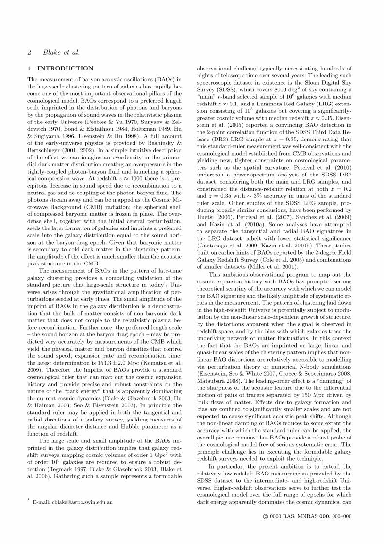
We determined the form of B(s) using halo cataloguesextracted from the GiggleZ dark matter simulation. ThisN -body simulation has been generated specifically in sup-port of WiggleZ survey science, and consists of 21603 par-ticles evolved in a 1 h−3 Gpc3 box using a WMAP5 cos-mology (Komatsu et al. 2009). We deduced B(s) using thenon-linear redshift-space halo correlation functions and non-linear dark-matter correlation function of the simulation.We found that a satisfactory fitting formula for the scale-dependent bias over the scales of interest is

B(s) = 1 + (s/s0)γ . (11)

We performed this procedure for several contiguous sub-sets of 250,000 halos rank-ordered by their maximum cir-cular velocity (a robust proxy for halo mass). The best-fitting parameters of Equation 11 for the subset which bestmatches the large-scale WiggleZ clustering amplitude ares0 = 0.32 h−1 Mpc, γ = −1.36. We note that the magnitudeof the scale-dependent correction from this term is ∼ 1%for a scale s ∼ 10 h−1 Mpc, which is far smaller than the∼ 10% magnitude of such effects for more strongly-biasedgalaxy samples such as Luminous Red Galaxies (Eisensteinet al. 2005). This greatly reduces the potential for system-atic error due to a failure to model correctly scale-dependentgalaxy bias effects.

3.4 Extraction of DV

We fitted the galaxy correlation function template modeldescribed above to the WiggleZ survey measurement, vary-

Figure 4. The scale-dependent correction to the non-linear real-space dark matter correlation function for haloes with maximumcircular velocity Vmax ≈ 125 km s−1, which possess the sameamplitude of large-scale clustering as WiggleZ galaxies. The greenline is the ratio of the real-space halo correlation function to thereal-space non-linear dark matter correlation function. The redline is the ratio of the redshift-space halo correlation functionto the real-space halo correlation function. The black line, theproduct of the red and green lines, is the scale-dependent biascorrection B(s) which we fitted with the model of Equation 11,shown as the dashed black line. The blue line is the ratio of thereal-space non-linear to linear correlation function.

ing the matter density Ωmh2, the scale distortion parame-ter α and the galaxy bias b2. Our default fitting range was10 < s < 180 h−1 Mpc (following Eisenstein et al. 2005),where 10 h−1 is an estimate of the minimum scale of va-lidity for the quasi-linear theory described in Section 3.3.In the following, we assess the sensitivity of the parameterconstraints to the fitting range.

We minimized the χ2 statistic using the full data co-variance matrix, assuming that the probability of a modelwas proportional to exp (−χ2/2). The best-fitting parame-ters were Ωmh2 = 0.132 ± 0.011, α = 1.075 ± 0.055 andb2 = 1.21±0.11, where the errors in each parameter are pro-duced by marginalizing over the remaining two parameters.The minimum value of χ2 is 14.9 for 14 degrees of freedom(17 bins minus 3 fitted parameters), indicating an accept-able fit to the data. In Figure 2 we compare the best-fittingcorrelation function model to the WiggleZ data points. Theresults of the parameter fits are summarized for ease of ref-erence in Table 1.

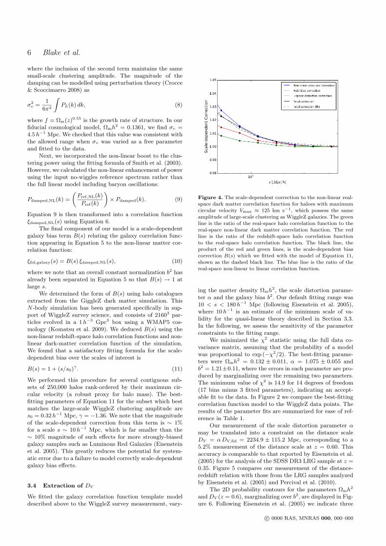
Our measurement of the scale distortion parameter αmay be translated into a constraint on the distance scaleDV = α DV,fid = 2234.9 ± 115.2 Mpc, corresponding to a5.2% measurement of the distance scale at z = 0.60. Thisaccuracy is comparable to that reported by Eisenstein et al.(2005) for the analysis of the SDSS DR3 LRG sample at z =0.35. Figure 5 compares our measurement of the distance-redshift relation with those from the LRG samples analyzedby Eisenstein et al. (2005) and Percival et al. (2010).

The 2D probability contours for the parameters Ωmh2

and DV (z = 0.6), marginalizing over b2, are displayed in Fig-ure 6. Following Eisenstein et al. (2005) we indicate three

c© 0000 RAS, MNRAS 000, 000–000


Figure 5. Measurements of the distance-redshift relation usingthe BAO standard ruler from LRG samples (Eisenstein et al. 2005,Percival et al. 2010) and the current WiggleZ analysis. The resultsare compared to a fiducial flat ΛCDM cosmological model withmatter density Ωm = 0.27.

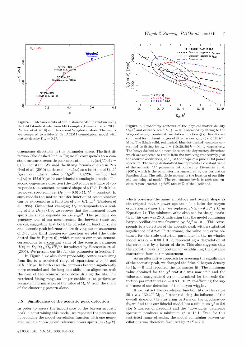
degeneracy directions in this parameter space. The first di-rection (the dashed line in Figure 6) corresponds to a con-stant measured acoustic peak separation, i.e. rs(zd)/DV (z =0.6) = constant. We used the fitting formula quoted in Per-cival et al. (2010) to determine rs(zd) as a function of Ωmh2

(given our fiducial value of Ωbh2 = 0.0226); we find thatrs(zd) = 152.6 Mpc for our fiducial cosmological model. Thesecond degeneracy direction (the dotted line in Figure 6) cor-responds to a constant measured shape of a Cold Dark Mat-ter power spectrum, i.e. DV (z = 0.6)×Ωmh2 = constant. Insuch models the matter transfer function at recombinationcan be expressed as a function of q = k/Ωmh2 (Bardeen etal. 1986). Given that changing DV corresponds to a scal-ing of k ∝ DV,fid/DV , we recover that the measured powerspectrum shape depends on DV Ωmh2. The principle de-generacy axis of our measurement lies between these twocurves, suggesting that both the correlation function shapeand acoustic peak information are driving our measurementof DV . The third degeneracy direction we plot (the dash-dotted line in Figure 6), which matches our measurement,corresponds to a constant value of the acoustic parameterA(z) ≡ DV (z)

√ΩmH2

0/cz introduced by Eisenstein et al.(2005). We present our fits for this parameter in Section 7.

In Figure 6 we also show probability contours resultingfrom fits to a restricted range of separations s > 30 and50 h−1 Mpc. In both cases the contours become significantlymore extended and the long axis shifts into alignment withthe case of the acoustic peak alone driving the fits. Therestricted fitting range no longer enables us to perform anaccurate determination of the value of Ωmh2 from the shapeof the clustering pattern alone.

3.5 Significance of the acoustic peak detection

In order to assess the importance of the baryon acousticpeak in constraining this model, we repeated the parameterfit replacing the model correlation function with one gener-ated using a “no-wiggles” reference power spectrum Pref(k),

Figure 6. Probability contours of the physical matter densityΩmh2 and distance scale DV (z = 0.6) obtained by fitting to theWiggleZ survey combined correlation function ξ(s). Results arecompared for different ranges of fitted scales smin < s < 180 h−1

Mpc. The (black solid, red dashed, blue dot-dashed) contours cor-respond to fitting for smin = (10, 30, 50) h−1 Mpc, respectively.The heavy dashed and dotted lines are the degeneracy directionswhich are expected to result from fits involving respectively justthe acoustic oscillations, and just the shape of a pure CDM powerspectrum. The heavy dash-dotted line represents a constant valueof the acoustic “A” parameter introduced by Eisenstein et al.(2005), which is the parameter best-measured by our correlationfunction data. The solid circle represents the location of our fidu-cial cosmological model. The two contour levels in each case en-close regions containing 68% and 95% of the likelihood.

which possesses the same amplitude and overall shape asthe original matter power spectrum but lacks the baryonoscillation features (i.e., we replaced PL(k) with Pref(k) inEquation 7). The minimum value obtained for the χ2 statis-tic in this case was 25.0, indicating that the model containingbaryon oscillations was favoured by ∆χ2 = 10.1. This corre-sponds to a detection of the acoustic peak with a statisticalsignificance of 3.2-σ. Furthermore, the value and error ob-tained for the scale distortion parameter in the no-wigglesmodel was α = 0.80 ± 0.17, representing a degradation ofthe error in α by a factor of three. This also suggests thatthe acoustic peak is important for establishing the distanceconstraints from our measurement.

As an alternative approach for assessing the significanceof the acoustic peak, we changed the fiducial baryon densityto Ωb = 0 and repeated the parameter fit. The minimumvalue obtained for the χ2 statistic was now 22.7 and thevalue and marginalized error determined for the scale dis-tortion parameter was α = 0.80± 0.12, re-affirming the sig-nificance of our detection of the baryon wiggles.

If we restrict the correlation function fits to the range50 < s < 130 h−1 Mpc, further reducing the influence of theoverall shape of the clustering pattern on the goodness-of-fit, we find that our fiducial model has a minimum χ2 = 5.9(for 5 degrees of freedom) and the “no-wiggles” referencespectrum produces a minimum χ2 = 13.1. Even for thisrestricted range of scales, the model containing baryon os-cillations was therefore favoured by ∆χ2 = 7.2.

c© 0000 RAS, MNRAS 000, 000–000

8 Blake et al.

3.6 Sensitivity to the clustering model

In this Section we investigate the systematic dependenceof our measurement of DV (z = 0.6) on the model used todescribe the quasi-linear correlation function. We consideredfive modelling approaches proposed in the literature:

• Model 1: Our fiducial model described in Section 3.3following Eisenstein et al. (2005), in which the quasi-lineardamping of the acoustic peak was modelled by an expo-nential factor g(k) = exp (−k2σ2

v), σv is determined fromlinear theory via Equation 8, and the small-scale power wasrestored by adding a term [1−g(k)] multiplied by the wiggle-free reference spectrum (Equation 7).• Model 2: No quasi-linear damping of the acoustic peak

was applied, i.e. σv = 0.• Model 3: The term restoring the small-scale power, [1−

g(k)]Pref(k) in Equation 7, was omitted.• Model 4: Pdamped(k) in Equation 7 was generated us-

ing Equation 14 of Eisenstein, Seo & White (2006), whichimplements different damping coefficients in the tangentialand radial directions.• Model 5: The quasi-linear matter correlation function

was generated using Equation 10 of Sanchez et al. (2009),following Crocce & Scoccimarro (2008), which includes theadditional contribution of a “mode-coupling” term. We setthe coefficient AMC = 1 in this equation (rather than intro-duce an additional free parameter).

Figure 7 compares the measurements of DV (z = 0.6)from the correlation function data, marginalized over Ωmh2

and b2, assuming each of these models. The agreementamongst the best-fitting measurements is excellent, and theminimum χ2 statistics imply a good fit to the data in eachcase. We conclude that systematic errors associated withmodelling the correlation function are not significantly af-fecting our results. The error in the distance measurementis determined by the amount of damping of the acousticpeak, which controls the precision with which the standardruler may be applied. The lowest distance error is producedby Model 2 which neglects damping; the greatest distanceerror is associated with Model 4, in which the damping isenhanced along the line-of-sight (see Equation 13 in Eisen-stein, Seo & White 2006).

4 POWER SPECTRUM

4.1 Measurements and covariance matrix

The power spectrum is a second commonly-used methodfor quantifying the galaxy clustering pattern, which is com-plementary to the correlation function. It is calculated us-ing a Fourier decomposition of the density field in which(contrary to the correlation function) the maximal signal-to-noise is achieved on large, linear or quasi-linear scales(at low wavenumbers) and the measurement of small-scalepower (at high wavenumbers) is limited by shot noise. How-ever, also in contrast to the correlation function, small-scaleeffects such as shot noise influence the measured power atall wavenumbers, and the baryon oscillation signature ap-pears as a series of decaying harmonic peaks and troughs atdifferent wavenumbers. In aesthetic terms this diffusion ofthe baryon oscillation signal is disadvantageous.

Figure 7. Measurements of DV (z = 0.6) from the galaxy corre-lation function, marginalizing over Ωmh2 and b2, comparing fivedifferent models for the quasi-linear correlation function as de-tailed in the text. The measurements are consistent, suggestingthat systematic modelling errors are not significantly affecting ourresults.

We estimated the galaxy power spectrum for each sep-arate WiggleZ survey region using the direct Fourier meth-ods introduced by Feldman, Kaiser & Peacock (1994; FKP).Our methodology is fully described in Section 3.1 of Blakeet al. (2010); we give a brief summary here. Firstly we mapthe angle-redshift survey cone into a cuboid of co-movingco-ordinates using a fiducial flat ΛCDM cosmological modelwith matter density Ωm = 0.27. We gridded the catalogue incells using nearest grid point assignment ensuring that theNyquist frequencies in each direction were much higher thanthe Fourier wavenumbers of interest (we corrected the powerspectrum measurement for the small bias introduced by thisgridding). We then applied a Fast Fourier transform to thegrid, optimally weighting each pixel by 1/(1 + nP0), wheren is the galaxy number density in the pixel (determined us-ing the selection function) and P0 = 5000 h−3 Mpc3 is acharacteristic power spectrum amplitude. The Fast Fouriertransform of the selection function is then used to constructthe final power spectrum estimator using Equation 13 inBlake et al. (2010). The measurement is corrected for theeffect of redshift blunders using Monte Carlo survey simula-tions as described in Section 3.2 of Blake et al. (2010). Wemeasured each power spectrum in wavenumber bins of width0.01 h Mpc−1 between k = 0 and 0.3 h Mpc−1, and deter-mined the covariance matrix of the measurement in thesebins by implementing the sums in Fourier space describedby FKP (see Blake et al. 2010 equations 20-22). The FKPerrors agree with those obtained from lognormal realizationswithin 10% at all scales.

In order to detect and fit for the baryon oscillation sig-nature in the WiggleZ galaxy power spectrum, we need tostack together the measurements in the individual survey re-gions and redshift slices. This requires care because each sub-region possesses a different selection function, and thereforeeach power spectrum measurement corresponds to a differ-ent convolution of the underlying power spectrum model.

c© 0000 RAS, MNRAS 000, 000–000


Table 1. Results of fitting a three-parameter model (Ωmh2, α, b2) to WiggleZ measurements of four different clustering statistics forvarious ranges of scales. The top four entries, above the horizontal line, correspond to our fiducial choices of fitting range for each statistic.The fitted scales α are converted into measurements of DV and two BAO distilled parameters, A and rs(zd)/DV , which are introducedin Section 7. The final column lists the measured value of DV when the parameter Ωmh2 is left fixed at its fiducial value and only the biasb2 is marginalized. We recommend using A(z = 0.6) as measured by the correlation function ξ(s) for the scale range 10 < s < 180 h−1

Mpc, highlighted in bold, as the most appropriate WiggleZ measurement for deriving BAO constraints on cosmological parameters.

Statistic Scale range Ωmh2 DV (z = 0.6) A(z = 0.6) rs(zd)/DV (z = 0.6) DV (z = 0.6)[Mpc] fixing Ωmh2

ξ(s) 10 < s < 180 h−1 Mpc 0.132± 0.011 2234.9± 115.2 0.452± 0.018 0.0692± 0.0033 2216.5± 78.9P (k) [full] 0.02 < k < 0.2 h Mpc−1 0.134± 0.008 2160.7± 132.3 0.440± 0.020 0.0711± 0.0038 2141.0± 97.5

P (k) [wiggles] 0.02 < k < 0.2 h Mpc−1 0.163± 0.017 2135.4± 156.7 0.461± 0.030 0.0699± 0.0045 2197.2± 119.1w0(r) 10 < r < 180 h−1 Mpc 0.130± 0.011 2279.2± 142.4 0.456± 0.021 0.0680± 0.0037 2238.2± 104.6

ξ(s) 30 < s < 180 h−1 Mpc 0.166± 0.014 2127.7± 127.9 0.475± 0.025 0.0689± 0.0031 2246.8± 102.6ξ(s) 50 < s < 180 h−1 Mpc 0.164± 0.016 2129.2± 140.8 0.474± 0.025 0.0690± 0.0031 2240.1± 104.7

P (k) [full] 0.02 < k < 0.1 h Mpc−1 0.150± 0.020 2044.7± 253.0 0.441± 0.034 0.0733± 0.0073 2218.1± 128.4P (k) [full] 0.02 < k < 0.3 h Mpc−1 0.137± 0.007 2132.1± 109.2 0.441± 0.017 0.0716± 0.0033 2148.9± 79.9

P (k) [wiggles] 0.02 < k < 0.1 h Mpc−1 0.160± 0.020 2240.7± 235.8 0.466± 0.034 0.0678± 0.0070 2277.9± 187.5P (k) [wiggles] 0.02 < k < 0.3 h Mpc−1 0.161± 0.019 2114.5± 132.4 0.455± 0.026 0.0706± 0.0037 2171.4± 98.0

w0(r) 30 < r < 180 h−1 Mpc 0.127± 0.018 2288.8± 157.3 0.455± 0.027 0.0681± 0.0037 2251.6± 111.7w0(r) 50 < r < 180 h−1 Mpc 0.164± 0.016 2190.0± 146.2 0.466± 0.023 0.0673± 0.0036 2282.1± 109.8

Furthermore the non-linear component of the underlyingmodel varies with redshift, due to non-linear evolution ofthe density and velocity power spectra. Hence the observedpower spectrum in general has a systematically-differentslope in each sub-region, which implies that the baryon os-cillation peaks lie at slightly different wavenumbers. If westacked together the raw measurements, there would be asignificant washing-out of the acoustic peak structure.

Therefore, before combining the measurements, wemade a correction to the shape of the various power spectrato bring them into alignment. We wish to avoid spuriouslyenhancing the oscillatory features when making this correc-tion. Our starting point is therefore a fiducial power spec-trum model generated from the Eisenstein & Hu (1998) “no-wiggles” reference linear power spectrum, which defines thefiducial slope to which we correct each measurement. Firstly,we modified this reference function into a redshift-space non-linear power spectrum, using an empirical redshift-space dis-tortion model fitted to the two-dimensional power spectrumsplit into tangential and radial bins (see Blake et al. 2011a).The redshift-space distortion is modelled by a coherent-flowparameter β and a pairwise velocity dispersion parameterσv, which were fitted independently in each of the redshiftslices. We convolved this redshift-space non-linear referencepower spectrum with the selection function in each sub-region, and our correction factor for the measured powerspectrum is then the ratio of this convolved function to theoriginal real-space linear reference power spectrum. Afterapplying this correction to the data and covariance ma-trix we combined the resulting power spectra using inverse-variance weighting.

Figures 8 and 9 respectively display the combined powerspectrum data, and that data divided through by the com-bined no-wiggles reference spectrum in order to reveal anysignature of acoustic oscillations more clearly. We note thatthere is a significant enhancement of power at the position ofthe first harmonic, k ≈ 0.075 h Mpc−1. The other harmonics

are not clearly detected with the current dataset, althoughthe model is nevertheless a good statistical fit. Figure 10displays the final power spectrum covariance matrix, result-ing from combining the different WiggleZ survey regions,in the form of a correlation matrix Cij/

√CiiCjj . We note

that there is very little correlation between separate 0.01 hMpc−1 power spectrum bins.

We note that our method for combining power spec-trum measurements in different sub-regions only corrects forthe convolution effect of the window function on the overallpower spectrum shape, and does not undo the smoothingof the BAO signature in each window. We therefore expectthe resulting BAO detection in the combined power spec-trum may have somewhat lower significance than that inthe combined correlation function.


We investigated two separate methods for fitting the scaledistortion parameter to the power spectrum data. Our firstapproach used the whole shape of the power spectrum in-cluding any baryonic signature. We generated a templatemodel non-linear power spectrum Pfid(k) parameterized byΩmh2, which we took as Equation 9 in Section 3.3, and fittedthe model

Pmod(k) = b2Pfid(k/α), (12)

where α now appears in the denominator (as opposed tothe numerator of Equation 5) due to the switch from realspace to Fourier space. As in the case of the correlation func-tion, the probability distribution of α, after marginalizingover Ωmh2 and b2, can be connected to the measurement ofDV (zeff). We determined the effective redshift of the powerspectrum estimate by weighting each pixel in the selectionfunction by its contribution to the power spectrum error:

c© 0000 RAS, MNRAS 000, 000–000

10 Blake et al.

Figure 8. The power spectrum obtained by stacking measure-ments in different WiggleZ survey regions using the method de-scribed in Section 4.1. The best-fitting power spectrum model(varying Ωmh2, α and b2) is overplotted as the solid line. Wealso show the corresponding “no-wiggles” reference model as thedashed line, constructed from a power spectrum with the sameclustering amplitude but lacking baryon acoustic oscillations.

Figure 9. The combined WiggleZ survey power spectrum of Fig-ure 8 divided by the smooth reference spectrum to reveal thesignature of baryon oscillations more clearly. We detect the firstharmonic peak in Fourier space.

zeff =∑

~x

z

(ng(~x)Pg

1 + ng(~x)Pg

)2

, (13)

where ng(~x) is the galaxy number density in each grid cell~x and Pg is the characteristic galaxy power spectrum am-plitude, which we evaluated at a scale k = 0.1 h Mpc−1. Weobtained an effective redshift zeff = 0.583. In order to enablecomparison with the correlation function fits we applied thebest-fitting value of α at z = 0.6.

Our second approach to fitting the power spectrummeasurement used only the information contained in thebaryon oscillations. We divided the combined WiggleZpower spectrum data by the corresponding combined no-

0.05 0.10 0.15 0.20ki [h Mpc−1 ]

0.05

0.10

0.15

0.20

kj [h M

pc−

1]

0.0

0.1

0.2

0.3

0.4

0.5

0.6

0.7

0.8

0.9

1.0

Corr

ela

tion C

oeff

icie

nt


CiiCjj

of the covariance matrix Cij for the power spectrum measure-ment, determined using the FKP estimator. The amplitude ofthe off-diagonal elements of the covariance matrix is very low.

wiggles reference spectrum, and when fitting models we di-vided each trial power spectrum by its corresponding refer-ence spectrum prior to evaluating the χ2 statistic.

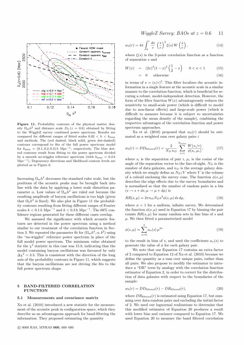
We restricted our fits to Fourier wavescales 0.02 < k <0.2 h Mpc−1, where the upper limit is an estimate of therange of reliability of the quasi-linear power spectrum mod-elling. We investigate below the sensitivity of the best-fittingparameters to the fitting range. For the first method, fittingto the full power spectrum shape, the best-fitting parame-ters and 68% confidence ranges were Ωmh2 = 0.134± 0.008and α = 1.050 ± 0.064, where the errors in each parameterare produced by marginalizing over the remaining two pa-rameters. The minimum value of χ2 was 12.4 for 15 degreesof freedom (18 bins minus 3 fitted parameters), indicatingan acceptable fit to the data. We can convert the constrainton the scale distortion parameter into a measured distanceDV (z = 0.6) = 2160.7± 132.3 Mpc. The 2D probability dis-tribution of Ωmh2 and DV (z = 0.6), marginalizing over b2,is displayed as the solid contours in Figure 11. In this Figurewe reproduce the same degeneracy lines discussed in Section3.4, which are expected to result from fits involving just theacoustic oscillations and just the shape of a pure CDM powerspectrum. We note that the long axis of our probability con-tours is oriented close to the latter line, indicating that theacoustic peak is not exerting a strong influence on fits to thefull WiggleZ power spectrum shape. Comparison of Figure11 with Figure 6 shows that fits to the WiggleZ galaxy cor-relation function are currently more influenced by the BAOsthan the power spectrum. This is attributable to the signalbeing stacked at a single scale in the correlation function, inthis case of a moderate BAO detection.

For the second method, fitting to just the baryon os-cillations, the best-fitting parameters and 68% confidenceranges were Ωmh2 = 0.163 ± 0.017 and α = 1.000 ± 0.073.Inspection of the 2D probability contours of Ωmh2 and α,which are shown as the dotted contours in Figure 11, indi-cates that a significant degeneracy has opened up parallelto the line of constant apparent BAO scale (as expected).

c© 0000 RAS, MNRAS 000, 000–000


Figure 11. Probability contours of the physical matter den-sity Ωmh2 and distance scale DV (z = 0.6) obtained by fittingto the WiggleZ survey combined power spectrum. Results arecompared for different ranges of fitted scales 0.02 < k < kmax

and methods. The (red dashed, black solid, green dot-dashed)contours correspond to fits of the full power spectrum modelfor kmax = (0.1, 0.2, 0.3) h Mpc−1, respectively. The blue dot-ted contours result from fitting to the power spectrum dividedby a smooth no-wiggles reference spectrum (with kmax = 0.2 hMpc−1). Degeneracy directions and likelihood contour levels areplotted as in Figure 6.

Increasing Ωmh2 decreases the standard ruler scale, but thepositions of the acoustic peaks may be brought back intoline with the data by applying a lower scale distortion pa-rameter α. Low values of Ωmh2 are ruled out because theresulting amplitude of baryon oscillations is too high (giventhat Ωbh2 is fixed). We also plot in Figure 11 the probabil-ity contours resulting from fitting different ranges of Fourierscales k < 0.1 h Mpc−1 and k < 0.3 h Mpc−1. The 68% con-fidence regions generated for these different cases overlap.

We assessed the significance with which acoustic fea-tures are detected in the power spectrum using a methodsimilar to our treatment of the correlation function in Sec-tion 3. We repeated the parameter fit for (Ωmh2, α, b2) usingthe “no-wiggles” reference power spectrum in place of thefull model power spectrum. The minimum value obtainedfor the χ2 statistic in this case was 15.8, indicating that themodel containing baryon oscillations was favoured by only∆χ2 = 3.3. This is consistent with the direction of the longaxis of the probability contours in Figure 11, which suggeststhat the baryon oscillations are not driving the fits to thefull power spectrum shape.

5 BAND-FILTERED CORRELATIONFUNCTION

5.1 Measurements and covariance matrix

Xu et al. (2010) introduced a new statistic for the measure-ment of the acoustic peak in configuration space, which theydescribe as an advantageous approach for band-filtering theinformation. They proposed estimating the quantity

w0(r) = 4π

∫ r

0

ds

r

(s

r

)2

ξ(s) W(

s

r

), (14)

where ξ(s) is the 2-point correlation function as a functionof separation s and

W (x) = (2x)2(1− x)2(

1

2− x

)0 < x < 1 (15)

= 0 otherwise (16)

in terms of x = (s/r)3. This filter localizes the acoustic in-formation in a single feature at the acoustic scale in a similarmanner to the correlation function, which is beneficial for se-curing a robust, model-independent detection. However, theform of the filter function W (x) advantageously reduces thesensitivity to small-scale power (which is difficult to modeldue to non-linear effects) and large-scale power (which isdifficult to measure because it is subject to uncertaintiesregarding the mean density of the sample), combining therespective advantages of the correlation function and powerspectrum approaches.

Xu et al. (2010) proposed that w0(r) should be esti-mated as a weighted sum over galaxy pairs i

w0(r) = DDfiltered(r) =2

ND nD

Npairs∑i=1

W (si/r)

φ(si, µi), (17)

where si is the separation of pair i, µi is the cosine of theangle of the separation vector to the line-of-sight, ND is thenumber of data galaxies, and nD is the average galaxy den-sity which we simply define as ND/V where V is the volumeof a cuboid enclosing the survey cone. The function φ(s, µ)describes the edge effects due to the survey boundaries andis normalized so that the number of random pairs in a bin(s → s + ds, µ → µ + dµ) is

RR(s, µ) = 2πnDNDs2φ(s, µ) ds dµ, (18)

where φ = 1 for a uniform, infinite survey. We determinedthe function φ(s, µ) used in Equation 17 by binning the paircounts RR(s, µ) for many random sets in fine bins of s andµ. We then fitted a parameterized model

φ(s, µ) =

3∑n=0

an(s) µ2n (19)

to the result in bins of s, and used the coefficients an(s) togenerate the value of φ for each galaxy pair.

We note that our Equation 17 contains an extra factorof 2 compared to Equation 12 of Xu et al. (2010) because wedefine the quantity as a sum over unique pairs, rather thanall pairs. We also propose to modify the estimator to intro-duce a “DR” term by analogy with the correlation functionestimator of Equation 2, in order to correct for the distribu-tion of data galaxies with respect to the boundaries of thesample:

w0(r) = DDfiltered(r)−DRfiltered(r), (20)

where DRfiltered(r) is estimated using Equation 17, but sum-ming over data-random pairs and excluding the initial factorof 2. We used our lognormal realizations to determine thatthis modified estimator of Equation 20 produces a resultwith lower bias and variance compared to Equation 17. Weused Equation 20 to measure the band filtered correlation

c© 0000 RAS, MNRAS 000, 000–000

12 Blake et al.

Figure 12. The band-filtered correlation function w0(r) for thecombined WiggleZ survey regions, plotted in the combinationr2w0(r). The best-fitting clustering model (varying Ωmh2, α andb2) is overplotted as the solid line. We also show the corresponding“no-wiggles” reference model, constructed from a power spectrumwith the same clustering amplitude but lacking baryon acousticoscillations. We note that the high covariance of the data pointsfor this estimator implies that (despite appearances) the solid lineis a good statistical fit to the data.

function of each WiggleZ region for 17 values of r spaced by10 h−1 Mpc between 15 and 175 h−1 Mpc.

We determined the covariance matrix Cij of our esti-mator using the ensemble of lognormal realizations for eachsurvey region. We note that for our dataset the amplitude ofthe diagonal errors

√Cii determined by lognormal realiza-

tions is typically ∼ 5 times greater than jack-knife errors and∼ 3 times higher than obtained by evaluating Equation 13in Xu et al. (2010) which estimates the covariance matrix inthe Gaussian limit. Given the likely drawbacks of jack-knifeerrors (the lack of independence of the jack-knife regions onlarge scales) and Gaussian errors (which fail to incorporatethe survey selection function), the lognormal errors shouldprovide by far the best estimate of the covariance matrix forthis measurement.

We constructed the final measurement of the band-filtered correlation function by stacking the individual mea-surements in different survey regions with inverse-varianceweighting. Figure 12 displays our measurement. We detectclear evidence of the expected dip in w0(r) at the acousticscale. Figure 13 displays the final covariance matrix of theband-filtered correlation function resulting from combiningthe different WiggleZ survey regions in the form of a corre-lation matrix Cij/

√CiiCjj . We note that the nature of the

w0(r) estimator, which depends on the correlation functionat all scales s < r, implies that the data points in differentbins of r are highly correlated, and the correlation coefficientincreases with r. At the acoustic scale, neighbouring 10 h−1

Mpc bins are correlated at the ∼ 85% level and bins spacedby 20 h−1 Mpc are correlated at a level of ∼ 55%.

50 100 150ri [h

−1 Mpc]

50

100

150

r j [h−

1 M

pc]

0.15

0.00

0.15

0.30

0.45

0.60

0.75

0.90

Corr

ela

tion C

oeff

icie

nt


CiiCjj

of the covariance matrix Cij for the band-filtered correlation func-tion measurement plotted in Figure 12, determined using lognor-mal realizations.


We determined the acoustic scale from the band-filteredcorrelation function by constructing a template functionw0,fid,galaxy(r) in the same style as Section 3.3 and then fit-ting the model

w0,mod(r) = b2 w0,fid,galaxy(α r). (21)

We determined the function w0,fid,galaxy(r) by applying thetransformation of Equation 14 to the template galaxy cor-relation function ξfid,galaxy(s) defined in Section 3.3, as afunction of Ωmh2.

The best-fitting parameters to the band-filtered corre-lation function are Ωmh2 = 0.130± 0.011, α = 1.100± 0.069and b2 = 1.32 ± 0.13, where the errors in each parameterare produced by marginalizing over the remaining two pa-rameters. The minimum value of χ2 is 10.5 for 14 degrees offreedom (17 bins minus 3 fitted parameters), indicating anacceptable fit to the data. Our measurement of the distor-tion parameter may be translated into a constraint on thedistance scale DV (z = 0.6) = αDV,fid = 2279.2±142.4 Mpc,corresponding to a 6.2% measurement of the distance scaleat z = 0.6. Probability contours of DV (z = 0.6) and Ωmh2

are overplotted in Figure 14.

In Figure 12 we compare the best fitting band-filteredcorrelation function model to the WiggleZ data points (not-ing that the strong covariance between the data gives themis-leading impression of a poor fit). We overplot a secondmodel which corresponds to our best-fit parameters but forwhich the no-wiggle reference power spectrum has been usedin place of the full power spectrum. If we fit this no-wigglesmodel varying Ωmh2, α and b2 we find a minimum valueof χ2 = 19.0, implying that the model containing acousticfeatures is favoured by ∆χ2 = 8.5.

c© 0000 RAS, MNRAS 000, 000–000


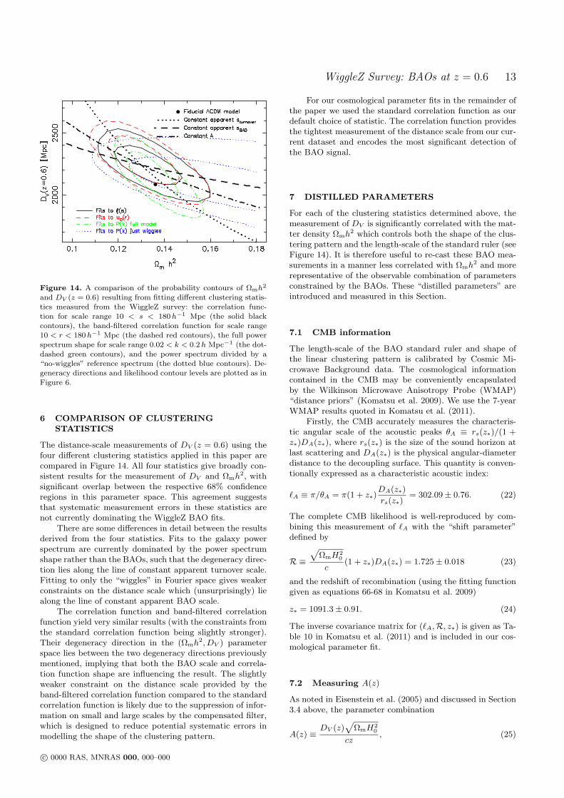
Figure 14. A comparison of the probability contours of Ωmh2

and DV (z = 0.6) resulting from fitting different clustering statis-tics measured from the WiggleZ survey: the correlation func-tion for scale range 10 < s < 180 h−1 Mpc (the solid blackcontours), the band-filtered correlation function for scale range10 < r < 180 h−1 Mpc (the dashed red contours), the full powerspectrum shape for scale range 0.02 < k < 0.2 h Mpc−1 (the dot-dashed green contours), and the power spectrum divided by a“no-wiggles” reference spectrum (the dotted blue contours). De-generacy directions and likelihood contour levels are plotted as inFigure 6.

6 COMPARISON OF CLUSTERINGSTATISTICS

The distance-scale measurements of DV (z = 0.6) using thefour different clustering statistics applied in this paper arecompared in Figure 14. All four statistics give broadly con-sistent results for the measurement of DV and Ωmh2, withsignificant overlap between the respective 68% confidenceregions in this parameter space. This agreement suggeststhat systematic measurement errors in these statistics arenot currently dominating the WiggleZ BAO fits.

There are some differences in detail between the resultsderived from the four statistics. Fits to the galaxy powerspectrum are currently dominated by the power spectrumshape rather than the BAOs, such that the degeneracy direc-tion lies along the line of constant apparent turnover scale.Fitting to only the “wiggles” in Fourier space gives weakerconstraints on the distance scale which (unsurprisingly) liealong the line of constant apparent BAO scale.

The correlation function and band-filtered correlationfunction yield very similar results (with the constraints fromthe standard correlation function being slightly stronger).Their degeneracy direction in the (Ωmh2, DV ) parameterspace lies between the two degeneracy directions previouslymentioned, implying that both the BAO scale and correla-tion function shape are influencing the result. The slightlyweaker constraint on the distance scale provided by theband-filtered correlation function compared to the standardcorrelation function is likely due to the suppression of infor-mation on small and large scales by the compensated filter,which is designed to reduce potential systematic errors inmodelling the shape of the clustering pattern.

For our cosmological parameter fits in the remainder ofthe paper we used the standard correlation function as ourdefault choice of statistic. The correlation function providesthe tightest measurement of the distance scale from our cur-rent dataset and encodes the most significant detection ofthe BAO signal.

7 DISTILLED PARAMETERS

For each of the clustering statistics determined above, themeasurement of DV is significantly correlated with the mat-ter density Ωmh2 which controls both the shape of the clus-tering pattern and the length-scale of the standard ruler (seeFigure 14). It is therefore useful to re-cast these BAO mea-surements in a manner less correlated with Ωmh2 and morerepresentative of the observable combination of parametersconstrained by the BAOs. These “distilled parameters” areintroduced and measured in this Section.

7.1 CMB information

The length-scale of the BAO standard ruler and shape ofthe linear clustering pattern is calibrated by Cosmic Mi-crowave Background data. The cosmological informationcontained in the CMB may be conveniently encapsulatedby the Wilkinson Microwave Anisotropy Probe (WMAP)“distance priors” (Komatsu et al. 2009). We use the 7-yearWMAP results quoted in Komatsu et al. (2011).

Firstly, the CMB accurately measures the characteris-tic angular scale of the acoustic peaks θA ≡ rs(z∗)/(1 +z∗)DA(z∗), where rs(z∗) is the size of the sound horizon atlast scattering and DA(z∗) is the physical angular-diameterdistance to the decoupling surface. This quantity is conven-tionally expressed as a characteristic acoustic index:

À ≡ π/θA = π(1 + z∗)DA(z∗)

rs(z∗)= 302.09± 0.76. (22)

The complete CMB likelihood is well-reproduced by com-bining this measurement of À with the “shift parameter”defined by

R ≡√

ΩmH20

c(1 + z∗)DA(z∗) = 1.725± 0.018 (23)

and the redshift of recombination (using the fitting functiongiven as equations 66-68 in Komatsu et al. 2009)

z∗ = 1091.3± 0.91. (24)

The inverse covariance matrix for (À,R, z∗) is given as Ta-ble 10 in Komatsu et al. (2011) and is included in our cos-mological parameter fit.

7.2 Measuring A(z)

As noted in Eisenstein et al. (2005) and discussed in Section3.4 above, the parameter combination

A(z) ≡DV (z)

√ΩmH2

0

cz, (25)

c© 0000 RAS, MNRAS 000, 000–000

14 Blake et al.

Figure 15. A comparison of the results of fitting different Wig-gleZ clustering measurements in the same style as Figure 14, ex-cept that we now fit for the parameter A(z = 0.6) (defined byEquation 25) rather than DV (z = 0.6).

which we refer to as the “acoustic parameter”, is particu-larly well-constrained by distance fits which utilize a com-bination of acoustic oscillation and clustering shape infor-mation, since in this situation the degeneracy direction ofconstant A(z) lies approximately perpendicular to the mi-nor axis of the measured (DV , Ωmh2) probability contours.Conveniently, A(z) is also independent of H0 (given thatDV ∝ 1/H0). Figure 15 displays the measurements result-ing from fitting the parameter set (A, Ωmh2, b2) to the fourWiggleZ clustering statistics and marginalizing over b2. Theresults of the parameter fits are displayed in Table 1; the cor-relation function yields A(z = 0.6) = 0.452±0.018 (i.e. witha measurement precision of 4.0%). For this clustering statis-tic in particular, the correlation between measurements ofA(z) and Ωmh2 is very low. Given that the CMB provides avery accurate determination of Ωmh2 (via the distance pri-ors) we do not use the WiggleZ determination of Ωmh2 inour cosmological parameter fits, but just use the marginal-ized measurement of A(z).

The measurement of A(z) involves the assumption ofa model for the shape of the power spectrum, which weparameterize by Ωmh2. Essentially the full power spectrumshape, rather than just the BAOs, is being used as a stan-dard ruler, although the two features combine in such a waythat A and Ωmh2 are uncorrelated. However, given that amodel for the full power spectrum is being employed, we re-fer to these results as large-scale structure (“LSS”) ratherthan BAO constraints, where appropriate.

7.3 Measuring dz

In the case of a measurement of the BAOs in which theshape of the clustering pattern is marginalized over, the(DV , Ωmh2) probability contours would lie along a line ofconstant apparent BAO scale. Hence the extracted distancesare measured in units of the standard-ruler scale, whichmay be conveniently quoted using the distilled parameterdz ≡ rs(zd)/DV (z) where rs(zd) is the co-moving sound

horizon size at the baryon drag epoch. In contrast to theacoustic parameter, dz provides a purely geometric distancemeasurement that does not depend on knowledge of thepower spectrum shape. The information required to com-pare the observations to theoretical predictions also variesbetween these first two distilled parameters: the predictionof dz requires prior information about h (or Ωmh2), whereasthe prediction of A(z) does not. We also fitted the parameterset (d0.6, Ωmh2, b2) to the four WiggleZ clustering statistics.The results of the parameter fits are displayed in Table 1;the correlation function yields d0.6 = 0.0692 ± 0.0033 (i.e.with a measurement precision of 4.8%). We note that, giventhe WiggleZ fits are in part driven by the shape of the powerspectrum as well as the BAOs, there is a weak residual cor-relation between d0.6 and Ωmh2.

When calculating the theoretical prediction for this pa-rameter we obtained the value of rs(zd) for each cosmologicalmodel tested using Equation 6 of Eisenstein & Hu (1998),which is a fitting formula for rs(zd) in terms of the valuesof Ωmh2 and Ωbh2. In our analysis we fixed Ωbh2 = 0.0226which is consistent with the measured CMB value (Komatsuet al. 2009); we find that marginalizing over the uncertaintyin this value does not change the results of our cosmologicalanalysis.

We note that rs(zd) is determined from the matter andbaryon densities in units of Mpc (not h−1 Mpc), and thus afiducial value of h must also be used when determining dz

from data (we chose h = 0.71). However, the quoted observa-tional result d0.6 = 0.0692± 0.0033 is actually independentof h. Adoption of a different value of h would result in ashifted standard ruler scale [in units of h−1 Mpc] and henceshifted best-fitting values of α and DV in such a way thatdz is unchanged. However, although the observed value ofdz is independent of the fiducial value of h, the model fittedto the data still depends on h as remarked above.

7.4 Measuring Rz

The measurement of dz may be equivalently expressed as aratio of the low-redshift distance DV (z) to the distance tothe last-scattering surface, exploiting the accurate measure-ment of À provided by the CMB. We note that the value ofRz depends on the behaviour of dark energy between red-shift z and recombination, whereas a constraint derived fromdz only depends on the properties of dark energy at redshiftslower than z. Taking the product of dz and À/π approx-imately cancels out the dependence on the sound horizonscale:

1/Rz ≡ À dz/π = (1 + z∗)DA(z∗)

rs(z∗)

rs(zd)

DV (z)(26)

≈ (1 + z∗)DA(z∗)

DV (z)× 1.044.

The value 1.044 is the ratio between the sound horizon atlast scattering and at the baryon drag epoch. Although thisis a model-dependent quantity, the change in redshift be-tween recombination and the end of the drag epoch is drivenby the relative number density of photons and baryons,which is a feature that does not change much across therange of viable cosmological models. Combining our mea-surement of d0.6 = 0.0692± 0.0033 from the WiggleZ corre-

c© 0000 RAS, MNRAS 000, 000–000


lation function fit with À = 302.09 ± 0.76 (Komatsu et al.2011) we obtain 1/R0.6 = 6.65± 0.32.

7.5 Measuring distance ratios

Finally, we can avoid the need to combine the BAO fits withCMB measurements by considering distance ratios betweenthe different redshifts at which BAO detections have beenperformed. Measurements of DV (z) alone are dependent onthe fiducial cosmological model and assumed standard-rulerscale: an efficient way to measure DV (z2)/DV (z1) is by cal-culating dz1/dz2 , which is independent of the value of rs(zd).Percival et al. (2010) reported BAO fits to the SDSS LRGsample in two correlated redshift bins d0.2 = 0.1905±0.0061and d0.35 = 0.1097 ± 0.0036 (with correlation coefficient0.337). Ratioing d0.2 with the independent measurement ofd0.6 = 0.0692 ± 0.0033 from the WiggleZ correlation func-tion and combining the errors in quadrature we find thatDV (0.6)/DV (0.2) = 2.753 ± 0.158. Percival et al. (2010)report DV (0.35)/DV (0.2) = 1.737 ± 0.065 (where in thislatter case the error is slightly tighter than obtained byadding errors in quadrature because of the correlation be-tween DV (0.2) and DV (0.35)). These two distance ratiomeasurements are also correlated by the common presenceof DV (0.2) in the denominators; the correlation coefficientis 0.313.

7.6 Comparison of distilled parameters

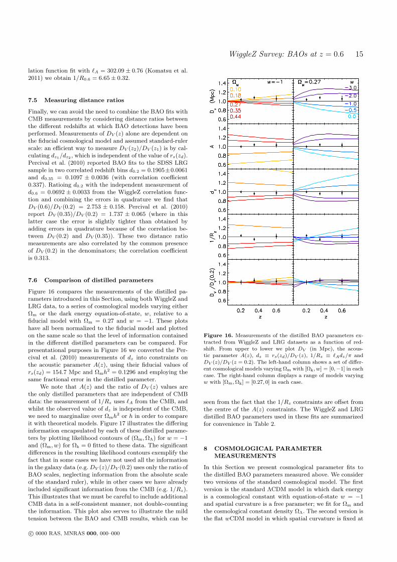
Figure 16 compares the measurements of the distilled pa-rameters introduced in this Section, using both WiggleZ andLRG data, to a series of cosmological models varying eitherΩm or the dark energy equation-of-state, w, relative to afiducial model with Ωm = 0.27 and w = −1. These plotshave all been normalized to the fiducial model and plottedon the same scale so that the level of information containedin the different distilled parameters can be compared. Forpresentational purposes in Figure 16 we converted the Per-cival et al. (2010) measurements of dz into constraints onthe acoustic parameter A(z), using their fiducial values ofrs(zd) = 154.7 Mpc and Ωmh2 = 0.1296 and employing thesame fractional error in the distilled parameter.

We note that A(z) and the ratio of DV (z) values arethe only distilled parameters that are independent of CMBdata: the measurement of 1/Rz uses À from the CMB, andwhilst the observed value of dz is independent of the CMB,we need to marginalize over Ωmh2 or h in order to compareit with theoretical models. Figure 17 illustrates the differinginformation encapsulated by each of these distilled parame-ters by plotting likelihood contours of (Ωm, ΩΛ) for w = −1and (Ωm, w) for Ωk = 0 fitted to these data. The significantdifferences in the resulting likelihood contours exemplify thefact that in some cases we have not used all the informationin the galaxy data (e.g. DV (z)/DV (0.2) uses only the ratio ofBAO scales, neglecting information from the absolute scaleof the standard ruler), while in other cases we have alreadyincluded significant information from the CMB (e.g. 1/Rz).This illustrates that we must be careful to include additionalCMB data in a self-consistent manner, not double-countingthe information. This plot also serves to illustrate the mildtension between the BAO and CMB results, which can be

Figure 16. Measurements of the distilled BAO parameters ex-tracted from WiggleZ and LRG datasets as a function of red-shift. From upper to lower we plot DV (in Mpc), the acous-tic parameter A(z), dz ≡ rs(zd)/DV (z), 1/Rz ≡ Àdz/π andDV (z)/DV (z = 0.2). The left-hand column shows a set of differ-ent cosmological models varying Ωm with [Ωk, w] = [0,−1] in eachcase. The right-hand column displays a range of models varyingw with [Ωm, Ωk] = [0.27, 0] in each case.

seen from the fact that the 1/Rz constraints are offset fromthe centre of the A(z) constraints. The WiggleZ and LRGdistilled BAO parameters used in these fits are summarizedfor convenience in Table 2.

8 COSMOLOGICAL PARAMETERMEASUREMENTS

In this Section we present cosmological parameter fits tothe distilled BAO parameters measured above. We considertwo versions of the standard cosmological model. The firstversion is the standard ΛCDM model in which dark energyis a cosmological constant with equation-of-state w = −1and spatial curvature is a free parameter; we fit for Ωm andthe cosmological constant density ΩΛ. The second version isthe flat wCDM model in which spatial curvature is fixed at

c© 0000 RAS, MNRAS 000, 000–000

16 Blake et al.

Figure 17. Likelihood contours (1-σ and 2-σ) derived from model fits to the different distilled parameters which may be used toencapsulate the BAO results from LRG and WiggleZ data. In each case the contours represent the combination of the three redshiftbins for which we have BAO data, z = [0.2, 0.35, 0.6]. The thick solid lines with grey shading show the A(z) parameter constraints,which are the most appropriate representation of WiggleZ data. The three sets of green lines show constraints from dz assuming threedifferent priors: green solid lines include a prior Ωmh2 = 0.1326 ± 0.0063 (Komatsu et al. 2009, as used by Percival et al. 2010); greendotted lines marginalize over a flat prior of 0.5 < h < 1.0; and green dashed lines marginalize over a Gaussian prior of h = 0.72± 0.03.Red dashed lines show the 1/Rz constraints, whilst fits to the ratios of BAO distances DV (z)/DV (0.2) are shown by blue dash-dotlines. The left-hand panel shows results for curved cosmological-constant universes parameterized by (Ωm, ΩΛ) and the right-hand paneldisplays results for flat dark-energy universes parameterized by (Ωm, w). Comparisons between these contours reveal the differing levels ofinformation encoded in each distilled parameter. By combining each type of distilled parameter with the CMB data in a correct manner,self-consistent results should be achieved.

Table 2. Measurements of the distilled BAO parameters at redshifts z = 0.2, 0.35 and 0.6 from LRG and WiggleZ data, which are usedin our cosmological parameter constraints. The LRG measurements at z = 0.2 and z = 0.35 are correlated with coefficient 0.337 (Percivalet al. 2010). The two distance ratios d0.2/d0.35 and d0.2/d0.6 are correlated with coefficient 0.313. The different measurements of 1/Rz

are correlated by the common presence of the `A variable and by the covariance between d0.2 and d0.35. Our default cosmological fitsuse the WiggleZ measurement of A(z = 0.6) combined with the LRG measurements of d0.2 and d0.35, indicated by bold font.

A(z) dz DV (z)/DV (0.2) 1/Rz

measured measured = d0.2/dz = `Adz/π

z = 0.2 (LRG) 0.488± 0.016 0.1905± 0.0061 — 18.32± 0.59z = 0.35 (LRG) 0.484± 0.016 0.1097± 0.0036 1.737± 0.065 10.55± 0.35

z = 0.6 (WiggleZ) 0.452± 0.018 0.0692± 0.0033 2.753± 0.158 6.65± 0.32

Ωk = 0 but the equation of state of dark energy is a freeparameter; we fit for Ωm and w.

Unless otherwise stated, we fitted these cosmologicalmodels to the WiggleZ measurement of A(z = 0.6) combinedwith the measurements of dz from LRG samples at z = 0.2and z = 0.35 (Percival et al. 2010). The distilled param-eter A(z) (measured from the galaxy correlation function)is the most appropriate choice for quantifying the WiggleZBAO measurement because it is uncorrelated with Ωmh2, asdemonstrated by Figure 15. The parameter dz provides thebest representation of the Percival et al. (2010) BAO data,because the shape of the clustering pattern was marginalizedover in that analysis.

8.1 BAO alone

As a first step in the cosmological analysis we consideredthe constraints on cosmological parameters obtained usingBAO data alone. Two of the distilled parameters allow thederivation of cosmological constraints based on only BAOmeasurements: the ratio of DV (z) measurements and theacoustic parameter, A(z).

Ratios of DV (z) measurements are of particularly inter-est because they provide constraints on the cosmic expan-sion history using geometric information alone, independentof the shape of the clustering pattern and the absolute scaleof the standard ruler. Plots of the resulting cosmologicalconstraints in our two test models (ΛCDM and wCDM) areshown in Figure 18. Using only LRG BAO data, the sin-

c© 0000 RAS, MNRAS 000, 000–000


Figure 18. Likelihood contours for cosmological parameter fits to BAO measurements using DV (z) distance ratios. We fit two differentmodels: curved cosmological-constant universes parameterized by (Ωm, ΩΛ) and flat dark-energy universes parameterized by (Ωm, w).Blue contours show the constraints using the measurement of DV (0.35)/DV (0.2) obtained by Percival et al. (2010). Red contours displaythe new constraints in DV (0.6)/DV (0.2) derived using WiggleZ data. The combination of these measurements is plotted as the greyshaded contours. One dimensional marginalized likelihoods for ΩΛ and w are displayed on the right-hand side of each contour plot. Inthe flat wCDM model, the BAO distance ratios alone require accelerating expansion (w < −1/3) with a likelihood of 99.8%. Comparedto the LRG data, WiggleZ does not favour as high values of ΩΛ or as negative values of w.

Figure 19. A comparison of the WiggleZ results and previous BAO measurements. The blue and green solid contours show theredshift z = 0.2 and z = 0.35 bins from Percival et al. (2010), using the dz parameter and including a CMB-motivated prior Ωmh2 =0.1326± 0.0063. The red contour displays the fit to the WiggleZ measurement of A(z) at z = 0.6, which is independent of any prior inΩmh2. We note that the degeneracy directions in these plots rotate with redshift, demonstrating the utility of combining measurementsat different redshifts. The grey shaded region shows the combination of d0.2 and d0.35 (including the correlation). The black solid linesare the 1, 2 and 3-σ contours of the final result combining all these BAO measurements. The addition of WiggleZ data reduces the 1-σuncertainty by about 50% in ΩΛ and about 30% in w, particularly disfavouring high values of ΩΛ and more negative values of w. We notethat in our final cosmological measurements we do not use a prior in Ωmh2 but instead combine our results with the WMAP distancepriors.

gle available distance ratio DV (0.35)/DV (0.2) provided rel-atively weak constraints on cosmological parameters and, inparticular, could not confirm the acceleration of the expan-sion of the universe. The addition of the second distance ra-tio based on WiggleZ data, DV (0.6)/DV (0.2), significantlyimproves these constraints. For the first time, purely geo-

metric distance ratios from BAO measurements demonstratethat the cosmic expansion is accelerating: assuming the flatwCDM model, a dark energy fluid with w < −1/3 is re-quired with a likelihood of 99.8% (assuming the flat prior−3 < w < 0).

The improvement in the χ2 statistic comparing the

c© 0000 RAS, MNRAS 000, 000–000

18 Blake et al.

best-fitting ΛCDM model (Ωm, ΩΛ) = (0.25, 1.1) to the Ein-stein de-Sitter model (Ωm, ΩΛ) = (1.0, 0.0) is ∆χ2 = 18,whilst comparing the best-fitting ΛCDM model to the openCDM model (Ωm, ΩΛ) = (0.27, 0.0) we obtain ∆χ2 = 8.Even given the extra parameter in the ΛCDM model, infor-mation criteria tests consider this level of improvement inχ2 to be significant evidence in favour of the ΛCDM modelcompared to a model with no dark energy.

Following the addition of the WiggleZ measurement, theBAO data alone require accelerating cosmic expansion witha higher level of statistical confidence than the initial lumi-nosity distance measurements from supernovae that are con-sidered to be the first direct evidence of accelerating expan-sion (compare the left-hand panel of Figure 18 with Figure 6of Riess et al. 1998). Although these BAO measurements arenot yet competitive with the latest supernova constraints,it is nevertheless reassuring that a standard-ruler measure-ment of the expansion of the universe, subject to an entirelydifferent set of potential systematic uncertainties, produces aresult in agreement with the standard-candle measurement.

The cosmological constraints from the acoustic param-eter A(z) are much more constraining than the DV (z) ratiosbecause they implicitly incorporate a model for the cluster-ing pattern and standard ruler scale as a function of Ωmh2.Figure 19 displays the resulting cosmological parameter fitsto the WiggleZ measurement of A(z = 0.6) combined withthe LRG measurements of dz=0.2,0.35. For the purposes ofthis Figure we combine the dz measurements with a priorΩmh2 = 0.1326 ± 0.0063 (following Percival et al. 2010);in the next sub-section we use the WMAP distance priorsinstead. The improvement delivered by the WiggleZ datacan be seen by comparing the shaded grey contour, whichis the combination of the LRG results, with the solid blackcontours representing the total BAO constraint includingthe new WiggleZ data. The current WiggleZ dataset de-livers an improvement of about 50% in the measurementof ΩΛ and about 30% in the measurement of w, based onLSS data alone. The marginalized parameter measurementsare Ωm = 0.25+0.05

−0.04 and ΩΛ = 1.1+0.2−0.4 (for ΛCDM) and

Ωm = 0.23± 0.06 and w = −1.6+0.6−0.7 (for wCDM).

The BAO results continue to prefer a more negativedark energy equation-of-state or a higher cosmological con-stant density than the CMB or supernovae data. We explorethis further in the following Section.

8.2 BAO combined with CMB and SNe

We now combine these large-scale structure (LSS) mea-surements with other cosmological datasets. We incorpo-rated the CMB data using the WMAP distance priors in(`A,R, z∗) described in Section 7.1. We fitted a model pa-rameterized by (Ωm, w, h) using flat priors 0.1 < Ωm < 0.5,0.5 < h < 1.0 and −3 < w < 0 and assuming a flat Uni-verse (Ωk = 0). Figure 20 compares the combined LSS cos-mological parameter measurements to the CMB constraintsin both the (Ωm, w) and (h, w) planes, marginalizing overh and Ωm respectively. The marginalized measurements ofeach parameter are Ωm = 0.287+0.029

−0.028, w = −0.982+0.154−0.189

and h = 0.692+0.044−0.038.

We also combined these constraints with those aris-ing from type Ia supernovae data from the “Union2” com-pilation by Amanullah et al. (2010), which includes data

from Hamuy et al. (1996), Riess et al. (1999, 2007), Astieret al. (2006), Jha et al. (2006), Wood-Vasey et al. (2007),Holtzman et al. (2008), Hicken et al. (2009) and Kessler etal. (2009). Using all of these data sets (LSS+CMB+SN)the best fitting wCDM model is (Ωm, w) = (0.284 ±0.016,−1.026 ± 0.081). This model provides a a good fit tothe data with a minimum χ2 per degree of freedom of 0.95.

The best-fitting parameter values based on LSS dataalone are offset by slightly more than one standard devi-ation from the best-fitting parameter values of the com-bined LSS+CMB+SN fit. This mild tension between LSSand CMB+SN results was already evident in the Percivalet al. (2007) measurement of BAOs in the SDSS: the LSSmeasurements prefer a slightly higher rate of acceleration,or a more negative equation of state of dark energy. The newWiggleZ results reported here serve to amplify that tension,although the level of discrepancy is not statistically signifi-cant.

In order to investigate whether more complex modelsgive a better statistical fit to these datasets we performed fitsof two additional cosmological models. The first is a wCDMmodel in which we allow curvature to be a free parameter;i.e. we fit for Ωm, Ωk and w. The second is a w(a)CDMmodel in which the equation-of-state of dark energy is al-lowed to vary linearly with scale factor (CPL parameteriza-tion; Chevallier & Polarski 2001, Linder 2003); i.e. we fit forΩm, w0, and wa. If these additional parameters are justifiedwe should find that the minimum value of the χ2 statisticdecreases significantly. However, we in fact find that the ad-dition of the extra degrees of freedom improves the χ2 valueof the best-fitting model by at most ∆χ2 = 0.6 compared tothe ΛCDM model, and significantly degrades the errors inour fitted parameters. In terms of information criteria thisdoes not represent a sufficient improvement to justify theaddition of the extra degree-of-freedom.

9 CONCLUSIONS

We summarize our conclusions as follows:

• This intermediate sample of the WiggleZ Dark EnergySurvey, containing N = 132,509 galaxies, permits a convinc-ing detection of baryon acoustic oscillations at the highestredshift achieved to date, z = 0.6. We have quantified thebaryon oscillations in both the galaxy correlation functionand power spectrum statistics. The statistical significance ofthe correlation function detection exceeds 3-σ.• We present the first measurement from a galaxy survey

of the band-filtered BAO estimator w0(r) defined by Xuet al. (2010), which also exhibits strong evidence of BAOs,and we suggest some improvements in its implementation.The distance-scale measurements resulting from w0(r) areslightly less precise than those obtained by fits to the stan-dard correlation function, likely due to the suppression bythe filtering function of clustering information on small andlarge scales.• The clustering statistics are well-fit by a non-linear

power spectrum model including a Gaussian damping fac-tor which models coherent flows on 100 h−1 Mpc scales. Weshow that our results are not sensitive to the details of thequasi-linear model by comparing five different implementa-tions suggested in the literature. We use the GiggleZ N-body

c© 0000 RAS, MNRAS 000, 000–000


Figure 20. Likelihood contours for cosmological parameter fits to LRG and WiggleZ BAO data, compared to and combined with CMBmeasurements. We have fitted for three parameters (Ωm, w and h) assuming a flat Universe. The left-hand panel of contours marginalizesover h and the right-hand panel of contours marginalizes over Ωm. The LSS constraints appear in blue, as dotted lines showing the Percivalet al. (2010) results for dz with no CMB prior, and as solid lines combining that data with the WiggleZ measurement of A(z). The redcontours show the CMB results (using the WMAP distance priors). The grey shaded contours display the combination of BAO and CMBmeasurements. One dimensional likelihood distributions for each of the parameters are shown as the insets. The BAO constraints shownhere are much wider than those plotted in Figure 19 because they do not assume any prior in Ωmh2. The improvement contributed bythe BAO, as compared to the CMB constraints alone, can be seen by comparing the black likelihood distributions, representing the totalconstraints, with the red likelihood distributions, which are for the CMB alone. (The sharp edges of the CMB likelihood distributionsarise due to the flat priors 0.5 < h < 1.0 and 0.1 < Ωm < 0.5 we adopted).

simulation to demonstrate that scale-dependent bias effectsin the WiggleZ galaxy distribution have an amplitude of 1%on 10 h−1 Mpc scales, compared to 10% for more highly-biased LRGs.

• We measured the distance-redshift relation DV (z =0.6) with an accuracy of about 5% using the scale di-lation method. The self-consistency of the measurementamongst the independent clustering statistics suggests thatsystematic measurement errors are not dominating theseresults. Our data best constrain the quantity A(z) =

DV (z)√

ΩmH20/cz, which lies perpendicular to the principal

degeneracy direction of our contours and which is measuredwith an accuracy of 4%: we find A(z = 0.6) = 0.452±0.018.

• The distance ratios between our measurements and pre-vious analyses of the Luminous Red Galaxy distribution atredshifts z = 0.2 and z = 0.35 are consistent with a flatΛCDM cosmological model which also provides a good fitto the CMB distance priors. Addition of the WiggleZ data

allows us to establish, using geometric distance ratios alone,that the equation-of-state of dark energy drives an accelerat-ing expansion (w < −1/3) with 99.8% likelihood, assuminga flat prior −3 < w < 0. The current WiggleZ dataset de-livers an improvement of about 50% in the measurement ofΩΛ and 30% in the measurement of w, based on BAO dataalone. The WiggleZ measurement confirms the mild tensionthat was previously reported between CMB and BAO mea-surements of the acceleration of the Universe, whereby theBAO data favour a slightly higher acceleration rate.

• Cosmological parameter fits using BAO and CMB dataare consistent with those based on current supernovae data;this cross-check does not yield evidence for systematic er-rors. Combining all current BAO, CMB and supernovae datawe find that the best-fitting wCDM model is (Ωm, w) =(0.284 ± 0.016,−1.026 ± 0.081). These data do not justifythe addition of another degree-of-freedom such as non-zero

c© 0000 RAS, MNRAS 000, 000–000

20 Blake et al.

spatial curvature or an evolving equation-of-state of darkenergy.

When the complete BAO dataset from the WiggleZ sur-vey is available, we plan to split our data into redshift binsand explore fitting for the BAOs separately in the tangen-tial and radial directions, improving the cosmological con-straints presented in this paper.

The WiggleZ dataset enables further tests of the cos-mological model, complementary to those involving baryonacoustic oscillations. Two such results will be published ata similar time as the current paper. Firstly, we have usedredshift-space distortions in the WiggleZ sample to measureaccurately the growth rate of structure in the redshift range0.1 < z < 0.9, finding that this is consistent with the pre-dictions of the ΛCDM model (Blake et al. 2011a). Secondly,we have used the Alcock-Paczynski test to perform non-parametric reconstructions of the cosmic expansion history(Blake et al. 2011b).

ACKNOWLEDGMENTS

We acknowledge financial support from the Australian Re-search Council through Discovery Project grants funding thepositions of SB, MP, GP and TD. SMC acknowledges thesupport of the Australian Research Council through a QEIIFellowship. MJD thanks the Gregg Thompson Dark EnergyTravel Fund for financial support.

GALEX (the Galaxy Evolution Explorer) is a NASASmall Explorer, launched in April 2003. We gratefully ac-knowledge NASA’s support for construction, operation andscience analysis for the GALEX mission, developed in co-operation with the Centre National d’Etudes Spatiales ofFrance and the Korean Ministry of Science and Technology.

Finally, the WiggleZ survey would not be possible with-out the dedicated work of the staff of the Australian Astro-nomical Observatory in the development and support of theAAOmega spectrograph, and the running of the AAT.

REFERENCES

Amanullah R., et al., 2010, ApJ, 716, 712

Astier P., et al., 2006, A&A, 447, 31

Bardeen J.M., Bond J.R., Kaiser N., Szalay A.S., 1986, ApJ, 304,15

Bashinsky S., Bertschinger E., 2001, Phys. Rev. Lett., 87, 081301

Bashinsky S., Bertschinger E., 2002, Phys. Rev. D, 65, 123008

Blake C.A, Glazebrook K., 2003, ApJ, 594, 665

Blake C.A., Parkinson D., Bassett B., Glazebrook K., Kunz M.,Nichol R.C., 2006, MNRAS, 365, 255

Blake C.A., Collister A., Bridle S., Lahav O., 2007, MNRAS, 374,1527

Blake C.A., et al., 2010, MNRAS, 406, 803

Blake C.A., et al., 2011a, MNRAS accepted

Blake C.A., et al., 2011b, MNRAS submitted

Bond J.R., Efstathiou G., 1984, ApJ, 285, L45

Chevallier M., Polarski D., 2001, Int. J. Mod. Phys., D10, 213

Cole S. et al., 2005, MNRAS, 362, 505

Coles P., Jones B., 1991, MNRAS, 248, 1

Crocce M., Scoccimarro R., 2008, Phys. Rev. D, 2008, 77, 3533

Drinkwater M., et al., 2010, MNRAS, 401, 1429

Eisenstein D.J., Hu W., 1998, ApJ, 518, 2

Eisenstein D.J. et al., 2005, ApJ, 633, 560

Eisenstein D.J., Seo H.-J., White M., 2007, ApJ, 664, 660Feldman H.A., Kaiser N., Peacock J.A., 1994, ApJ, 426, 23Gaztanaga E., Cabre A., Hui L., 2009, MNRAS, 399, 1663Glazebrook K., Blake C.A., 2005, ApJ, 631, 1Hamuy M., et al., 1996, AJ, 112, 2408Hicken M., et al., 2009, ApJ, 700, 331Holtzman J.A., 1989, ApJS, 71, 1Holtzman J.A., et al. 2008, AJ, 136, 2306Hu W., Haiman Z., 2003, Phys. Rev. D, 68, 063004Hu W., Sugiyama N., 1996, ApJ, 471, 542Huetsi G., 2006, A&A, 449, 891Jha S., et al., 2006, AJ, 131, 527Kazin E., et al., 2010a, ApJ, 710, 1444Kazin E., Blanton M.R., Scoccimarro R., McBride C.K., Berlind

A.A., 2010b, ApJ, 719, 1032Kessler R., et al., 2009, ApJS, 185, 32Komatsu E., et al., 2009, ApJS, 180, 330Komatsu E., et al., 2011, ApJS, 192, 18Landy S.D., Szalay A.S., 1993, ApJ, 412, 64Lewis A., Challinor A., Lasenby A., 2000, ApJ, 538, 473Linder E.V., 2003, PRL, 90, 091301Matsubara T., 2008, Phys. Rev. D, 78, 083519Miller C.J., Nichol R.C., Batuski D.J., 2001, ApJ, 555, 68Padmanabhan N. et al., 2007, MNRAS, 378, 852Padmanabhan N., White M., 2008, Phys. Rev. D, 77, 3540Peebles P.J.E., Yu J.T., 1970, ApJ, 162, 815Peebles P.J.E., 1980, The Large-Scale Structure of the Universe,

Princeton Univ. Press, Princeton, NJPercival W.J., et al., 2007, ApJ, 657, 51Percival W.J., et al., 2010, MNRAS, 401, 2148Riess A.G., et al., 1998, AJ, 116, 1009Riess A.G., et al., 1999, AJ, 117, 707Riess A.G., et al., 2007, ApJ, 659, 98Sanchez A.G., Crocce M., Cabre A., Baugh C.M., Gaztanaga E.,

2009, MNRAS, 400, 1643Seo H.-J., Eisenstein D.J., 2003, ApJ, 598, 720Smith R.E. et al., 2003, MNRAS, 341, 1311Sunyaev R.A., Zeldovitch, Y.B., 1970, Ap&SS, 7, 3Tegmark M., 1997, PRL, 79, 20Wood-Vasey W.M., et al., 2007, ApJ, 666, 694Xu X., et al., 2010, ApJ, 718, 1224

c© 0000 RAS, MNRAS 000, 000–000

the wigglez dark energy survey: testing the cosmological...

Documents