the volatility and density prediction performance of alternative garch models

Journal of ForecastingJ. Forecast. 31, 157–171 (2012)Published online 28 January 2011 in Wiley Online Library(wileyonlinelibrary.com) DOI: 10.1002/for.1217

The Volatility and Density PredictionPerformance of AlternativeGARCH Models

TENG-HAO HUANG1 AND YAW-HUEI WANG2*1 National Central University, Taoyuan, Taiwan2 National Taiwan University, Taipei, Taiwan

ABSTRACTThis study compares the volatility and density prediction performance of alter-native GARCH models with different conditional distribution specifications.The conditional residuals are specified as normal, skewed-t or compoundPoisson (jump) distribution based upon a nonlinear and asymmetric GARCH(NGARCH) model framework. The empirical results for the S&P 500 and FTSE100 index returns suggest that the jump model outperforms all other models interms of both volatility forecasting and density prediction. Nevertheless, thesuperiority of the non-normal models is not always significant and diminishedduring the sample period on those occasions when volatility experiences anobvious structural change. Copyright © 2011 John Wiley & Sons, Ltd.

KEY WORDS GARCH; volatility forecasting; density prediction; skewed-t ;jump

INTRODUCTION

Volatility can be defined and interpreted in numerous ways, such as realized volatility, conditionalvolatility, and implied volatility. However, since it is a measure of price uncertainty, the forecastingof volatility is important for investment, derivatives valuation and risk management. While a volatilityforecast is a number which provides only partial information about the distribution of the future priceof an asset, a far more challenging task which can be of further benefit to derivatives traders and riskmanagers alike involves the use of market information to predict the entire distribution of the futureasset price.

Density prediction is a different problem from volatility prediction but is related to it. Whencertain simulation or bootstrap techniques are applied, both tasks can be executed simulta-neously with an asset price dynamic model. Although both volatility and density forecasts can beobtained from historical and/or option prices, the focus of this study is necessarily placed upon

* Correspondence to: Yaw-Huei Wang, College of Management, National Taiwan University, No. 1, Section 4, RooseveltRoad, Taipei 10617, Taiwan. E-mail: [email protected]

Copyright © 2011 John Wiley & Sons, Ltd.

158 T.-H. Huang and Y.-H. Wang

the historical models;1 and indeed, amongst the various streams of the historical models, the gen-eralized autoregressive conditional heteroskedasticity (GARCH)-type models, initiated by Engle(1982), extended by Bollerslev (1986) and Taylor (1986), and subsequently followed by manyothers, have proven to be the most successful models for describing and predicting asset pricedynamics.

The success of the GARCH-type models comes as a result of their ability to capture many of thestylized facts of financial asset returns.2 Although the conditional distribution of returns in a GARCH-type model is typically assumed to be normal, from their review of numerous studies Poon andGranger (2003) concluded that the standardized residuals from most GARCH-type models continuedto display significant kurtosis. In other words, the higher-order features of the conditional distributionhave tended to be completely ignored (Hansen, 1994); as a result, substantial return shocks may tendto be under-fitted by the normal models.

The literature aimed at providing a remedy for this problem has assumed at least two direc-tions.3 The first approach was to directly model the stylized facts in the stochastic residuals witha flexible density (Bollerslev, 1987; Nelson, 1991; Hansen, 1994), while the second approachhas attempted to capture the unusual and sudden changes in prices by including jump dynam-ics (Maheu and McCurdy, 2004; Duan et al., 2006, 2007). To this end, it would seem naturalto ask whether these efforts can always significantly improve the performance of the GARCH-type models in terms of certain economic applications, although they are of course necessary forsuperiority in an econometric sense. We therefore regard this study as contributing to the litera-ture through its provision of a comprehensive comparison of alternative GARCH-type models (withdifferent conditional distribution specifications) in terms of their volatility and density predictionperformance.

As the asymmetric news impact has been well known for equity assets, the empirical com-parison presented here is based upon the nonlinear and asymmetric GARCH (NGARCH) frame-work proposed by Engle and Ng (1993), with the standardized residuals being assumed to benormal, to investigate whether assuming the residuals to be (i) following skewed-t distribution(Hansen, 1994) or (ii) adapting to sudden return shocks by including jump dynamics (Duan et al.,2006, 2007) can improve the precision of volatility and density prediction. Hence this study usesthe traditional normal model (NGARCH-normal) as the benchmark to explore the incrementalcontribution of the non-normal specifications, comprising the skewed-t (NGARCH- skewed-t/and jump (NGARCH-jump) models, in volatility and density prediction for the S&P 500 andFTSE 100 indices.

1 Poon and Granger (2003) provided a comprehensive review of volatility forecasting, while there has been extensive investi-gation into density prediction in many studies over recent years, such as Ritchey (1990), Madan and Milne (1994), Jackwerthand Rubinstein (1996), Melick and Thomas (1997), Malz (1996, 1997), Campa et al. (1998), Jondeau and Rockinger (2000),Rosenberg and Engle (2002), Bliss and Panigirtzoglou (2002), Liu et al. (2007), Wang (2009) and Shackleton et al. (2010),most of which were based upon the theoretical results for complete markets derived by Breeden and Litzenberger (1978); thustheir focus was on option-implied densities.2 As indicated by Taylor (2005), there are at least four general properties that can be found in almost all sets of daily returns forfinancial assets, with the GARCH-type models having the capability of capturing them all. Firstly, the distribution of returnsis non-normal; secondly, there is almost no correlation between returns for different days; thirdly, there is positive dependencebetween absolute/squared returns on nearby days; and fourthly, good news and bad news have different impacts on futurevolatility—the phenomenon referred to as asymmetry.3 An alternative way of making the models more realistic is to increase the volatility memory length (Bollerslev and Mikkelsen,1996); however, the information set used to form conditional volatility in this type of long-memory model differs from that ofa short-memory model; therefore, no long-memory model is included in this study so as to avoid any unfair comparisons.

Copyright © 2011 John Wiley & Sons, Ltd. J. Forecast. 31, 157–171 (2012)DOI: 10.1002/for

Volatility and Density Prediction 159

Based on 10,000 repeats of simulated prices and volatility values for many rolling samples,4 ourempirical results for various forecasting horizons reveal that the return processes are better describedby the non-normal specifications. Furthermore, the NGARCH-jump model is found to outperform theothers in terms of both volatility forecasting and density prediction, although the achievement in thelatter of these is less significant. Nevertheless, the advantages of these non-normal models on bothapplications are diminished for certain sample periods, in particular a period characterized by low,stable volatility. It may therefore be necessary to detect any structural changes in volatility, and toadapt to these when employing any of the historical models for time series modeling and forecasting,such as the GARCH-type models. Otherwise, a more complicated model that requires a much heaviercomputation load may not be superior to a simple one.

The remainder of this paper is organized as follows. The three volatility models employed in thisstudy are described in detail in the next section, followed in the third section by presentation ofthe measures used to evaluate the volatility forecasting and density prediction performance of thevarious models. The fourth section presents the data used for our empirical analysis, with the analysissubsequently being presented in the fifth section along with a discussion of the results. Finally, theconclusions drawn from this study are presented in the sixth section.

EMPIRICAL MODELS

Many types of GARCH models, such as the EGARCH (Nelson, 1991), NGARCH (Engle and Ng,1993) and GJR (Glosten et al., 1993) models, are capable of capturing the asymmetric news impactthat has been well documented for equity returns. As the focus of this study is on the distributionalspecifications of residuals (rather than the dynamic specifications of conditional variance) and thejump model we follow (Duan et al., 2006, 2007) is specified for the NGARCH model, we simplyuse the NGARCH-normal model of Engle and Ng (1993) as the benchmark to investigate whetherthe NGARCH-skewed-t and the NGARCH-jump models can improve the precision of volatility anddensity prediction.5 This section provides details of the specifications and estimation procedures ofthe alternative models in a nested framework.6

Let {rt} denote the daily return process, and It�1 be the information set comprising of all of theprevious returns. The generalized NGARCH process is defined by

rt D ˛t C h1=2

t Jt (1)

where Jt �D.�J , �J , �0/, and

4 Miguel and Olave (1999) and Pascual et al. (2006) use bootstrap approaches to predict volatility and density simultaneously.In particular, Pascual et al. (2006) incorporate parameter uncertainty and overcome the need for distributional assumptions.However, the procedure requires re-estimating parameters for every replication and thus using this approach will be extremelytime-consuming for a complicated model like NGARCH-jump because it usually takes hours to finish one estimation pro-cedure. The analysis here is therefore based on the results produced by conventional simulation techniques. Nonetheless, tocheck the robustness of our empirical findings, the results obtained from the approaches of Miguel and Olave (1999) andPascual et al. (2006) will be compared with those generated by the conventional simulation procedure.5 We also use the GJR framework for our empirical comparison and find that the results are very similar to those under theNGARCH framework. However, the levels of log-likelihood produced by the NGARCH-type models are higher than thoseobtained under the GJR-type models.6 It is very important to have similar models when doing this kind of comparison.



ht D ˇ0C ˇ1ht�1C ˇ2ht�1

�Jt�1 ��J

�J� c

�2(2)

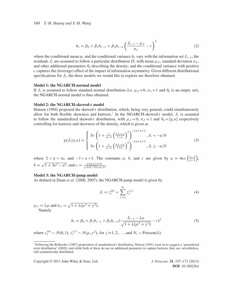
where the conditional mean ˛t and the conditional variance ht vary with the information set It�1; theresiduals Jt are assumed to follow a particular distribution D, with mean �J , standard deviation �J ,and other additional parameters �0 describing the density; and the conditional variance with positivec captures the (leverage) effect of the impact of information asymmetry. Given different distributionalspecifications for Jt , the three models we would like to explore are therefore obtained.

Model 1: the NGARCH-normal modelIf Jt is assumed to follow standard normal distribution (i.e. �JD0, �JD1 and �0 is an empty set),the NGARCH-normal model is thus obtained.

Model 2: the NGARCH-skewed-t modelHansen (1994) proposed the skewed-t distribution, which, being very general, could simultaneouslyallow for both flexible skewness and kurtosis.7 In the NGARCH-skewed-t model, Jt is assumedto follow the standardized skewed-t distribution, with �J D0, �J D1 and �0D Œ�, �� respectivelycontrolling for kurtosis and skewness of the density, which is given as

g.Jt j�, �/D

8̂̂<ˆ̂:bc

�1C 1

��2

�bJtCa

1��

�2��.�C1/=2,Jt < �a=b

bc

�1C 1

��2

�bJtCa

1C�

�2��.�C1/=2,Jt � �a=b

(3)

where 2 < � <1, and �1< �<1. The constants a, b, and c are given by a D 4�c��2

��1

�,

b Dp1C 3�2 � a2, and c D Γ..�C1/=2/

p�.��2/Γ.�=2/

.

Model 3: the NGARCH-jump modelAs defined in Duan et al. (2006, 2007), the NGARCH-jump model is given by

Jt D ´.0/

t C

NtXjD1

´.j/t (4)

�J D �� and �J Dp1C �.�2C 2/.

Namely

ht D ˇ0C ˇ1ht�1C ˇ2ht�1.Jt�1 � ��p1C �.�2C 2/

� c/2 (5)

where ´.0/t �N.0, 1/, ´.j/t �N.�, 2/, for jD1, 2, : : :, and Nt � Poisson.�/.

7 Following the Bollerslev (1987) proposition of standardized t distribution, Nelson (1991) went on to suggest a ‘generalizederror distribution’ (GED), and while both of these do use an additional parameter to capture kurtosis, they are, nevertheless,still symmetrically distributed.



The compound Poisson is employed to handle the arrival of unusual news events which have animpact on returns.8 The jump sizeZ.j/t is normally distributed with mean� and variance 2, while thenumber of jumps Nt is an invisible variable of non-negative integral with the arrival intensity � beingnon-negative. It should be noted that unless � D 0, the mean (variance) of Jt will not be 0 (1), butinstead �� and 1C�.�2C2/, respectively. The normalized Jt�1..Jt�1��/=

p1C �.�2C 2// in

the last term of equation (5) serves to make this equation comparable to the NGARCH-normal model,which typically uses a random variable with mean 0 and variance 1 (Duan et al., 2007). Intuitively,the existence of frequent large positive or negative return shocks indicates �>0 and brings signifi-cant kurtosis to the conditional distribution. A higher frequency of negative shocks, as compared topositive shocks, implies �<0 and left skewness.9 Obviously, specifying a non-normal distributionfor, and including jump dynamics in, the standardized residuals, both lead to the same consequence:a much more flexible conditional distribution of returns.

The ‘maximum likelihood estimation’ (MLE) method is employed to estimate the parameters forall models. The conditional density of the returns f .rt jIt�1, ™/ can be obtained by transforming thedensity of the standardized residuals Zt . Given that ht and Zt are functions of subset �1�� and thatthe density of Zt is determined by the subset �2�� , where �1[ �2D� , the log-likelihood functionof rt is

logL.� jr1, : : : , rn/DnXtD1

�1

2log.ht.�1//C log.f .´t.�1/j�2// (6)

The density of Zt in the NGARCH-normal model is a standard normal; therefore, �2D¿.The density of Zt in the NGARCH-skewed-t model is a standardized skewed-t density; therefore,�2D f�, �g. The conditional density of rt in the NGARCH-jump model is, however, more compli-

cated since it includes two random variables (i.e. Z.0/t andNtPjD1

´.j/t /; thus the conditional density ofrt in the NGARCH-jump model is given as10

f .rt jIt�1, �/D1XkD0

�k exp.��/

kŠN.˛t C kuh

1=2

t , ht.1C k2// (7)

PERFORMANCE EVALUATION

As compared to the NGARCH-normal model, the performance of the non-normal models is evaluatedin terms of the precision of the volatility forecasting and density prediction. Not only are we able to

8 To capture any unexpected and significant reductions or increases in price, Press (1967) introduced a basic compound eventsmodel, in which unusual news events followed the Poisson process and the size of such movements was assumed to be normal.This jump idea has since been employed in GARCH-type models by Vlaar and Palm (1993), Chan and Maheu (2002), Maheuand McCurdy (2004), and Duan et al. (2006, 2007).9 If the arrival intensity is allowed to be time-variant, the conditional skewness and conditional kurtosis will also be time-varying; however, Duan et al. (2007) indicated that in their model the variability of the arrival intensity was trivial. We alsoestimate the model with the time-varying arrival intensity following the specification of Maheu and McCurdy (2004) and ourresults coincide with the indication of Duan et al. (2007).10 As suggested by Maheu and McCurdy (2004) and Duan et al. (2007), infinity in equation (7) is proxied by 50, which islarge enough to make the summation converge.



obtain a set of simulated returns from the simulation procedure, but also a set of simulated vari-ances. Therefore, we can evaluate the performance of alternative models on both volatility and densityprediction from the same simulation procedure.

Volatility forecastingFor a GARCH-type model, given It , the one-period forecast (htC1/will be immediately known, whiletheH -period forecast can be obtained either from a simulation procedure or by taking the conditionalexpectation of the sum ofH -conditional variances. For consistency with the procedure used to predictdensity, the empirical analysis is based on the simulated results.11

Although there is only one random term per unit of time in the NGARCH-normal and theNGARCH-skewed-t models, we nevertheless have to simulate three random terms in the NGARCH-jump model. Based on the simulated variance values {htC1,htC2, . . . , htCH}, theH -period simulatedvariance can be computed as hH D htC1ChtC2C ...ChtCH . By repeating the simulation procedure10,000 times, we can obtain 10,000 simulated values of hH . The H -period volatility forecast is thesquare root of their mean.

The realized volatility calculated under the Andersen et al. (2001) approach is used as the targetfor forecasting; specifically, the daily realized variance is defined as the sum of the squared 5-minutereturns during the day, and thus the total realized volatility over H days is the square root of the sumof H daily realized variances.12

We not only use the ‘mean squared error’ (MSE) and ‘root mean squared error’ (RMSE) values,but also, as suggested by Diebold and Mariano (1995), employ Wilcoxon’s signed-rank test for eval-uation of the forecasting performance of the alternative models. By rolling over a fixed-length sampleperiod for parameter estimation m times, we have m forecasts for a particular horizon, H .

The MSE and RMSE are respectively defined as 1mmPjD1

.fj ,H � yj ,H /2 and

s1m

mPjD1

�fj ,H�yj ,H

yj ,H

�2,

where fj ,H and yj ,H respectively denote the j th forecast and realized volatility values over H days.To further compare the forecasting power statistically, we use Wilcoxon’s signed-rank test for the null

hypothesis that the median of forecasting errors, measured by .fj ,H �yj ,H /2 or

�fj ,H�yj ,H

yj ,H

�2, for the

tested model is not less than that of the benchmark model. The test statistic is

SDmXtD1

IC.dt/rank.jdt j/ (8)

where dt is the forecasting error of the tested model minus that of the benchmark model at time t .IC.dt/ = 1 if dt > 0, otherwise IC.dt/ D 0. Moreover, its standardized version is asymptoticallystandard normal:

Sa DS � m.mC1/

4qm.mC1/.2mC1/

24

�aN.0, 1/ (9)

11 The volatility forecasts generated from the latter approach will be compared later for the robustness check.12 According to Andersen et al. (2001), the 5-minute frequency is an appropriate choice due to the tradeoff betweenmicrostructure effects and measurement precision.



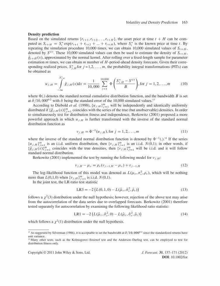
Density predictionBased on the simulated returns frtC1, rtC2, : : :, rtCH g, the asset price at time t C H can be com-puted as StCH D S�t exp.rtC1 C rtC2 C ... C rtCH /, where S�t is the known price at time t . Byrepeating the simulation procedure 10,000 times, we can obtain 10,000 simulated values of StCH ,denoted by S .i/. These 10,000 simulated values can then be used to estimate the density of StCH ,OgtCH .x/, approximated by the normal kernel. After rolling over a fixed-length sample for parameterestimationm times, we can obtainm number ofH -period-ahead density forecasts. Given their corre-sponding realized prices, S�

j ,H for j =1,2, . . . , m, the probability integral transformations (PITs) canbe obtained as

uj ,H D

S�j ,HZ�1

Ogj ,H .x/dx D1

10, 000

10,000XiD1

Φ

S�j ,H � S

.i/

B

!, for j D 1, 2, : : : ,m (10)

where Φ(.) denotes the standard normal cumulative distribution function, and the bandwidth B is setat O�=10, 0000.2 with O� being the standard error of the 10,000 simulated values.13

According to Diebold et al. (1998), fuj ,H gmjD1 will be independently and identically uniformly

distributed if f Ogj ,H .x/gmjD1 coincides with the series of the true (but unobservable) densities. In order

to simultaneously test for distribution fitness and independence, Berkowitz (2001) proposed a morepowerful approach in which uj ,H is further transformed with the inverse of the standard normaldistribution function as

j ,H D Φ�1.uj ,H /, for j D 1, 2, : : : ,m (11)

where the inverse of the standard normal distribution function is denoted by Φ�1(.).14 If the seriesfuj ,H g

mjD1 is an i.i.d. uniform distribution, then fj ,H g

mjD1 is an i.i.d. N (0,1); in other words, if

f Ogj ,H .x/gmjD1 coincides with the true densities, then fj ,H g

mjD1 will be i.i.d. and it will follow

standard normal distribution.Berkowitz (2001) implemented the test by running the following model for j ,H :

j ,H �� D ��.j�1,H ��/C "j�1,H (12)

The log-likelihood function of this model was denoted as L.�� , �2� , ��/, which will be nothingmore than L(0,1,0) when fj ,H g

mjD1 is i.i.d. N (0,1).

In the joint test, the LR-ratio test statistic

LR3D�2�L.0, 1, 0/�L. O�� , O�2� , O��/

�(13)

follows a �2(3) distribution under the null hypothesis; however, rejection of the above test may arisefrom the autocorrelation of the data series due to overlapped forecasts. Berkowitz (2001) thereforetested separately for autocorrelation by examining the following likelihood ratio statistic:

LR1D�2�L. O�� , O�2� , 0/�L. O�� , O�2� , O��/

�(14)

which follows a �2(1) distribution under the null hypothesis.

13 As suggested by Silverman (1986), it is acceptable to set the bandwidth at O�=10,0000.2 since the standardized returns haveunit variance.14 Many other tests, such as the Kolmogorov–Smirnof test and the Anderson–Darling test, can be employed to test fordistribution fitness only.



If Ogj ,H .x/ provides accurate density, we cannot reject the null of LR3 and LR1. Conversely, if LR3is rejected, this leads to two circumstances. Firstly, if LR1 is also rejected, the rejection of LR3 may bedue to the series autocorrelation of the forecasts and it will therefore prove difficult to make any deci-sion. Secondly, if LR1 is not rejected, then we can conclude that the estimated density is inaccurate.

DATA

Our empirical investigation is conducted on the S&P 500 and the FTSE 100 indices for a sampleperiod running from 1 May 1997 to 29 April 2005. The primary dataset comprises of the high-frequency (5-minute) levels of these two indices obtained from Olsen. The closing price of a singletrading day is taken from the last intraday price of the day.

The single-period returns are defined by the logarithmic price change, and thus the multi-period returns are the sums of the single-period returns. While the intraday returns are usedto compute realized volatility, the daily returns are used as the inputs for the GARCH-typemodels.

Consistent with the stylized facts for equity returns found in many of the prior studies such asAndersen et al. (2001) and Areal and Taylor (2002), both the S&P 500 and the FTSE 100 indexreturns are negatively skewed and leptokurtic. The Jarque–Bera statistics further suggest that thereturn distributions of both indices are non-Gaussian.

While there appears to be no high autocorrelation for the daily returns of the S&P 500 index,the autocorrelations at lags 2 and 3 are slightly negative for the FTSE 100 index (�0.05 and �0.1,respectively). The results of the likelihood ratio tests do not, however, provide support for any particu-lar specification for the conditional means of the returns of both indices.15 As a result, the conditionalmeans of the returns for both indices are assumed to be constant in the following analyses.

The daily realized volatility series of the S&P 500 and the FTSE 100 indices are plotted inFigure 1, from which it is clearly evident that volatility clustering is present in both indices, withthe volatility having been relatively stable and low over recent years, from about April 2003. Sincethe occurrence of extreme values seems to have been less frequent during this period, it may be quiteinteresting to explore whether the advantage of a model is dependent upon the volatility structure.This issue will be examined later in this study.

EMPIRICAL RESULTS

We apply three models to the daily returns of the S&P 500 and the FTSE 100 indices, using theNGARCH-normal model as the benchmark. Our study aims to examine whether the non-normalmodels, motivated under different perspectives, can provide any improvement on either volatility ordensity prediction. Before doing so, we first briefly summarize the model estimation or fitting results.

The MLE procedure is used to estimate the parameters in the models, with the likelihood-ratio(LR) tests and the Akaike information criteria (AIC) being used to evaluate the performance of the

15 For example, for the FTSE 100 index returns, the log-likelihoods for the NGARCH- normal model with the conditionalmean specified as AR(1), MA(1), and ARMA(1,1) are 6250.22, 6250.22 and 6251.88, respectively, which are only slightlyhigher than the likelihood from the model with a constant conditional mean (6250.21).



0

0.2

0.4

0.6

0.8

1

1.2

1.4

1.6

1.8

1997

05

1997

10

1998

04

1998

10

1999

04

1999

10

2000

04

2000

09

2001

03

2001

09

2002

03

2002

09

2003

03

2003

09

2004

03

2004

09

2005

03

Date

Ann

ualiz

ed R

ealiz

ed V

olat

ility

S&P 500 FTSE 100

Figure 1. Annualized realized volatility. The figure shows the realized volatility series of the S&P 500 and theFTSE indices for the sample period from 1 May 1997 to 29 April 2005; all volatility values are annualized

three models in terms of model fitting. Consistent with previous studies such as Bollerslev (1987),Nelson (1991), Glosten et al. (1993) and Poon and Granger (2003), the estimates of parameters revealmany well-known properties of price dynamics of equity assets, including the inappropriateness ofthe normality assumption, the existence of volatility clustering and leverage effect, and the station-arity of the volatility processes. In general, the non-normal models have both higher log-likelihoodand lower AIC values than the NGARCH-normal model, and indeed the LR tests also support thenon-normal specifications of the conditional distribution.

The empirical results for volatility forecasting and density prediction are detailed in the followingtwo subsections and followed by further discussion and robustness analysis.

Volatility forecastingWe take the observations for the last 3 years of the sample period as the out-of-sample period. Thetotal volatility over the five horizons of 1, 5, 10, 20 and 30 days are forecast under the three alternativemodels, with the whole sample being exhausted by the use of the rolling procedure. The MSE andRMSE values based on the realized volatility and the standardized statistics of the Wilcoxon’s signed-rank test based on the NGARCH-normal model are presented in Table I for the S&P 500 index, andin Table II for the FTSE 100 index.

The non-normal models generally outperform the normal model, with the NGARCH-jump modelperforming best of all, which is dependent on neither the assets nor the forecasting horizons. In par-ticular, in terms of MSE (RMSE), the jump model improves volatility forecasting performance in theS&P 500 index by as much as 12.70% (7.52%) to 17.61% (9.74%). However, while the skewed-tmodel performs rather well in terms of model fitting, its performance in volatility forecasting is less



Table I. Volatility forecasting performance, S&P 500

Model Horizon

1 day 5 days 10 days 20 days 30 days

Panel A: MSENGARCH-normal 0.00244 0.00176 0.00197 0.00250 0.00298NGARCH-skewed-t 0.00242 0.00173 0.00194 0.00248 0.00298

(–3.40) (–6.00) (–6.67) (–5.93) (–4.19)NGARCH-jump 0.00213 0.00145 0.00164 0.00213 0.00260

(–16.71) (–18.94) (–19.78) (–18.72) (–17.28)

Panel B: RMSENGARCH-normal 0.4347 0.3447 0.3554 0.4025 0.4461NGARCH-skewed-t 0.4302 0.3402 0.3507 0.3984 0.4429

(–4.98) (–6.98) (–7.67) (–6.74) (–5.42)NGARCH-jump 0.4020 0.3122 0.3207 0.3655 0.4084

(–19.20) (–20.63) (–21.42) (–21.17) (–20.30)

Note: Panel A presents the mean squared errors of volatility forecasting for the S&P 500 index returns, while panel B presentsthe root mean squared relative errors. The out-of-sample period runs from 1 May 2002 to 29 April 2005. Values in paren-theses refer to the standardized statistics of Wilcoxon’s signed-rank test for the improvement in forecasting based on theNGARCH-normal model.

Table II. Volatility forecasting performance, FTSE 100

Model Horizon

1 day 5 days 10 days 20 days 30 days

Panel A: MSENGARCH-normal 0.00311 0.00211 0.00230 0.00300 0.00356NGARCH-skewed-t 0.00302 0.00204 0.00224 0.00292 0.00345

(–0.60) (–1.74) (–2.95) (–3.22) (–2.02)NGARCH-jump 0.00291 0.00191 0.00209 0.00274 0.00325

(–8.59) (–9.69) (–10.37) (–11.35) (–10.74)

Panel B: RMSENGARCH-normal 0.4213 0.3327 0.3501 0.4034 0.4548NGARCH-skewed-t 0.4179 0.3286 0.3458 0.4008 0.4541

(–2.46) (–3.73) (–4.22) (–3.44) (–1.95)NGARCH-jump 0.3867 0.2991 0.3140 0.3634 0.4126

(–12.55) (–14.23) (–15.03) (–16.28) (–16.06)

Note: Panel A presents the mean squared errors of volatility forecasting for the FTSE 100 index returns, while panel Bpresents the root mean squared relative errors. The out-of-sample period runs from 1 May 2002 to 29 April 2005. Values inparentheses refer to the standardized statistics of Wilcoxon’s signed-rank test for the improvement in forecasting based on theNGARCH-normal model.

convincing. For both criteria under all horizons, the percentages of forecasting improvement made bythe slewed-t model are less than 1.52%, with the one exception of 30-day forecasting in the S&P 500index. Similar results can also be found for the FTSE 100 index.

These findings are also confirmed by the Wilcoxon’s signed-rank test. Based on the NGARCH-normal model, the NGARCH-jump model has significantly lowered the forecasting errors for both



indices under all horizons with the significance levels less than 1%. However, the absolute valuesof the test statistics for the NGARCH-skewed-t model are much lower and sometimes the improve-ment in reducing forecasting errors is even insignificant under the significance level of 10% (1-dayforecasting for the FTSE 100 index).

In summary, the NGARCH-jump model outperforms the other models, in terms of volatil-ity forecasting performance, for both indices and for all forecasting horizons. This finding isconsistent with that of Maheu and McCurdy (2004), although the jump component is specifieddifferently.

Density predictionDensity prediction is also executed for the five horizons of 1, 5, 10, 20 and 30 days, with the Berkowitz(2001) approach being used to evaluate the performance of the alternative NGARCH models. Tenthousand simulated values are generated to form each density, and in order to avoid producing over-lapping forecasts the forecasts are formed once per unit of horizon. For example, for the 5-dayforecast, the forecasts are formed once every 5 days.16 The results of the Berkowitz (2001) testsare presented in Table III.

The results for the S&P 500 index presented in panel A of Table III suggest that all three modelsfail to provide accurate predictions for the 1-day densities, given that the LR3 statistics are rejectedunder the significance level of 5% but the LR1 statistics are not. All three models provide accurateestimated densities for other horizons, since all LR3 statistics are smaller than the critical value underthe significance level of 5% (7.81), as are all LR1 statistics (3.84).

Thus, under the significance level of 5%, there appears to be no significant difference between thethree models, in terms of their density prediction performance; however, under the significance levelof 10%, the p-values suggest that the skewed-t and jump models provide good prediction for 5-daydensities, whereas the normal model does not.

Furthermore, for all horizons (with the exception of the 20-day horizon), the LR3 statistics pro-duced by the skewed-t and jump models are smaller than those produced by the normal model.According to Berkowitz (2001), a smaller (higher) LR3 statistic value (p-value) implies more accuratedensity prediction; hence it is reasonable to suggest that the non-normal models provide more accu-rate density prediction than the normal model, although such prediction superiority is not statisticallysignificant.

The results for the FTSE 100 index presented in panel B of Table III are quite similar to thosefor the S&P 500 index. For the 10-, 20- and 30-day forecasts, all three models provide accurate esti-mated densities, given the rejection of the nulls of LR3 and LR1 under the significance level of 5%.However, under the significance level of 1%, only the NGARCH-jump model provides satisfactorydensity prediction for the 1-day forecasts. We therefore continue to assert that the non-normal modelsprovide more accurate density prediction than the normal model. In addition, for all horizons, the LR3statistics produced by the skewed-t and jump models are smaller than those produced by the normalmodel.

Thus it seems that capturing the higher-order features of conditional density can indeed improvethe performance of density prediction, which is consistent with the finding of Wang (2009) usingoption-implied densities.

16 The total numbers of observations for the S&P 500 index are: 1-day forecasts (732); 5-day forecasts (147); 10-day forecasts(74); 20-day forecasts (37); and 30-day forecasts (25). The total numbers of observations for the FTSE 100 index are: 1-dayforecasts (758); 5-day forecasts (152); 10-day forecasts (76); 20-day forecasts (38); and 30-day forecasts (26).



Table III. Density prediction evaluation

Horizon NGARCH-normal NGARCH-skewed-t NGARCH-jump

LR3 LR1 LR3 LR1 LR3 LR1

Panel A: S&P 5001 day 10.63 2.85 8.38 2.65 8.17 2.59

(0.0139) (0.0915) (0.0387) (0.1036) (0.0426) (0.1073)5 days 6.36 0.11 6.03 0.11 6.11 0.20

(0.0953) (0.7416) (0.1099) (0.7422) (0.1062) (0.6515)10 days 4.11 0.37 3.71 0.33 3.91 0.19

(0.2498) (0.5425) (0.2944) (0.5666) (0.2710) (0.6631)20 days 3.12 0.08 2.82 0.07 3.55 0.12

(0.3732) (0.7758) (0.4202) (0.7977) (0.3137) (0.7315)30 days 3.44 0.88 3.27 0.84 3.31 0.80

(0.3287) (0.3469) (0.3521) (0.3599) (0.3468) (0.3698)

Panel B: FTSE 1001 day 13.07 4.63 11.81 4.64 10.36 5.04

(0.0045) (0.0314) (0.0081) (0.0312) (0.0158) (0.0248)5 days 10.54 0.47 8.53 0.30 7.96 0.15

(0.0145) (0.4910) (0.0362) (0.5814) (0.0468) (0.6951)10 days 4.33 0.27 3.85 0.23 3.64 0.06

(0.2275) (0.6032) (0.2778) (0.6309) (0.3035) (0.8079)20 days 2.58 0.31 2.54 0.38 2.34 0.21

(0.4603) (0.5765) (0.4688) (0.5378) (0.5048) (0.6433)30 days 4.34 1.28 3.92 1.13 3.73 0.82

(0.2265) (0.2582) (0.2706) (0.2884) (0.2919) (0.3640)

Note: The table presents the LR3 and LR1 statistics of Berkowitz (2001), with the LR3 statistics following a chi-square distri-bution with three degrees of freedom under the null hypothesis that the estimated densities coincide with the true densities, andthe LR1 statistics following a chi-square distribution with one degree of freedom under the null hypothesis. Values in paren-theses are p-values. The out-of-sample period runs from 1 May 2002 to 29 April 2005, with the forecast horizons covering1-day, 5-day, 10-day, 20-day and 30-day periods; the forecasts for all horizons are non-overlapped. The decision criteria forthe tests are: (i) if the nulls of both the LR3 and LR1 statistics are not rejected, then the estimated densities provide accurateforecasts; (ii) if the null of the LR3 statistic is rejected, but the null of the LR1 statistic is not, the estimated densities providepoor forecasts; and (iii) if the nulls of both the LR3 and the LR1 statistics are rejected, we are unable to draw any conclusion.

Further discussionAs shown in Figure 1, the volatility processes for both indices have been relatively stable andlow over recent years; thus, in order to determine whether this phenomenon affects the ade-quacy of the non-normal densities, we divide the whole sample period evenly, and reinvesti-gate the volatility and density prediction performance of the three models for the two resultantsubsamples.

Overall, the results for the second subsample, with stable, low volatility, differ significantly fromthe results for the whole sample and the first subsample, and the advantage of the non-normal modelsseems to be reduced substantially. Volatility is generally overestimated even by the NGARCH-jumpmodel for the second subsample. In particular, the forecasting errors of the S&P 500 index for thesecond half of the sample period are about 1.6 times those for the first half. Similarly, for the sec-ond subsample, all three models provide poor density prediction for all horizons, with all of the LR3



statistics being larger than the critical values under the significance level of 5%, whereas the LR1statistics are not.17

We may therefore suggest that the normal model may be appropriate for recent years, a period inwhich volatility became stably low, and the advantage of the non-normal models was quite limited.Namely, extreme events may be relatively unimportant for this period.18

In fact, the failure of all three models to provide good volatility and density prediction for theperiod with volatility becoming stably low is an inevitable shortcoming of virtually all historicalmodels, and we may need to take into account structural changes in volatility when employing suchhistorical models for volatility and density prediction.

Robustness analysisIt should be noted that not only can volatility forecasts be generated by the simulation procedure butalso by the analytical solutions derived from taking the conditional expectations of the sum of H -conditional variances. Therefore, the simulation results of volatility forecasting from the simulationare compared with those from the analytical solutions, not only as a means of checking the robustnessof our empirical results but also as a means of checking the quality of our simulation.

The MSEs and RMSEs of the alternative models for the two forecasting approaches show that thevolatility forecasts from the simulation are almost identical to those from the analytical solutions.In particular, the maximum RMSE difference for the S&P 500 index is only 0.0003. Our empiricalresults and simulation procedures are therefore deemed to be reliable.

Although the bootstrap procedure proposed by Pascual et al. (2006) can integrate volatility fore-casting and density prediction, overcome the need for the distributional assumption and incorporateparameter uncertainty, it is too computationally expensive for our study, especially for the NGARCH-jump model. Nonetheless, to further ensure the robustness of our empirical findings, we use 1000repeats to check whether the distributions of price and volatility forecasts produced by our simulationprocedure are different from those generated by the approaches of Pascual et al. (2006) as well asMiguel and Olave (1999).

The summary statistics of the distributions generated by alternative approaches show that the meanlevels (of both volatility and price forecasts) do not obviously differ. In particular, the difference involatility (price) for the S&P 500 index is smaller than 0.01 (5) in general. However, the differencebetween the 5% and 95% percentiles is generally wider for the distributions produced by the bootstrapprocedure of Pascual et al. (2006), which is regarded as a natural outcome of incorporating parameteruncertainty. These robustness findings do not depend on the forecasting horizon.

In summary, our empirical findings are robust to the approaches used to generate volatility andprice forecasts.

CONCLUSIONS

In an attempt to incorporate the higher-order features of the conditional distribution in the GARCHclass models, we can either directly model the stylized facts in the stochastic residuals, with some

17 Since the sample period is divided into two equal parts, there are too few observations for 20- and 30-day forecasts; thus theforecasts for these two horizons are omitted here.18 There is a rich literature on extreme-value-based tail estimation and density prediction. For example, see Longin (2000),McNeil and Frey (2000), Bali (2003, 2007) and Jalal and Rockinger (2008).



flexible densities, or make some attempt to capture the unusual changes in prices by including jumpdynamics. In order to examine whether these adjustment approaches can provide any improvement interms of volatility and density prediction performance as compared to the normal model, in this studywe have implemented the NGARCH-normal, NGARCH-skewed-t and NGARCH-jump models forthe S&P 500 and the FTSE 100 indices. We find that the non-normal models generally outperform thenormal model in all respects, although their level of superiority in density prediction is not statisticallysignificant.

However, we have also found that all of the advantages of the non-normal models over the normalmodel are substantially reduced when they are applied to any sample period that is characterized bystable and low volatility. In fact, a rather inevitable shortcoming of all the historical models is that theout-of-sample forecasts will tend to be seriously biased if there is any structural change in volatility.It may therefore be necessary to attempt to design a mechanism capable of adapting to structuralchanges when attempting to employ such historical models for volatility and density prediction. Thisis an issue that must be left to future research.

ACKNOWLEDGEMENTS

We are indebted to the seminar participants at National Chengchi University, National Dong HwaUniversity, National Taiwan University, and the 20th Australasian Finance and Banking Conferencein Sydney. We are also grateful to the National Science Council of Taiwan for the financial supportprovided for this study.

REFERENCES

Andersen TG, Bollerslev T, Diebold FX, Ebens H. 2001. The distribution of realized stock return volatility. Journalof Financial Economics 61: 43–76.

Areal NMPC, Taylor SJ. 2002. The realized volatility of FTSE-100 futures prices. Journal of Futures Markets 22:627–648.

Bali TG. 2003. An extreme value approach to estimating volatility and value at risk. Journal of Business 76: 83–108.Bali TG. 2007. A generalized extreme value approach to financial risk measurement. Journal of Money, Credit and

Banking 39: 1613–1649.Berkowitz J. 2001. Testing density forecasts, with applications to risk management. Journal of Business and

Economic Statistics 19: 465–674.Bliss RR, Panigirtzoglou N. 2002. Testing the stability of implied probability density functions. Journal of Banking

and Finance 26: 381–422.Bollerslev T. 1986. Generalized autoregressive conditional heteroskedasticity. Journal of Econometrics 31:

307–327.Bollerslev T. 1987. A conditionally heteroskedastic time-series model for speculative prices and rates of return.

Review of Economics and Statistics 69: 542–547.Bollerslev T, Mikkelsen H. 1996. Modeling and pricing long memory in stock market volatility. Journal of

Econometrics 73: 151–184.Breeden D, Litzenberger R. 1978. Prices of state-contingent claims implicit in options prices. Journal of Business

51: 621–651.Campa JM, Chang PH, Reider RL. 1998. Implied exchange rate distributions: evidence from OTC option markets.

Journal of International Money and Finance 17: 117–160.Chan WH, Maheu JM. 2002. Conditional jump dynamics in stock market returns. Journal of Business and Economic

Statistics 20: 377–389.



Diebold FX, Mariano RS. 1995. Comparing predictive accuracy. Journal of Business and Economic Statistics 13:253–263.

Diebold FX, Gunther TA, Tay AS. 1998. Evaluating density forecasts with applications to financial riskmanagement. International Economic Review 39: 863–883.

Duan JC, Ritchken P, Sun Z. 2006. Approximating GARCH-jump model, jump-diffusion processes and optionpricing. Mathematical Finance 16: 21–52.

Duan JC, Ritchken P, Sun Z. 2007. Jump starting GARCH: pricing and hedging options with jumps in returns andvolatilities. Working paper, Toronto University.

Engle RF. 1982. Autoregressive conditional heteroscedasticity with estimates of the variance of United Kingdominflation. Econometrica 50: 987–1007.

Engle RF, Ng VK. 1993. Measuring and testing the impact of news on volatility. Journal of Finance 48: 1749–1778.Glosten LR, Jagannathan R, Runkle DE. 1993. On the relation between the expected value and the volatility of the

nominal excess return on stocks. Journal of Finance 48: 1779–1801.Hansen BE. 1994. Autoregressive conditional density estimation. International Economic Review 35: 705–730.Jackwerth JC, Rubinstein M. 1996. Recovering probability distributions from option prices. Journal of Finance 51:

1611–1631.Jalal A, Rockinger M. 2008. Predicting tail-related risk measures: the consequences of using GARCH filters for

non-GARCH data. Journal of Empirical Finance 15: 868–877.Jondeau E, Rockinger M. 2000. Reading the smile: the message conveyed by methods which infer risk-neutral

densities. Journal of International Money and Finance 19: 885–915.Liu X, Shackleton M, Taylor SJ, Xu X. 2007. Closed-form transformations from risk-neutral to real-world

distributions. Journal of Banking and Finance 31: 1501–1520.Longin FM. 2000. From value at risk to stress testing: the extreme value approach. Journal of Banking and Finance

24: 1097–1130.Madan DB, Milne F. 1994. Contingent claims valued and hedged by pricing and investing in a basis. Mathematical

Finance 4: 223–245.Maheu JM, McCurdy TH. 2004. News arrival, jump dynamics and volatility components for individual stock

returns. Journal of Finance 59: 755–793.Malz A. 1996. Using option prices to estimate realignment probabilities in the European Monetary System: the case

of sterling–mark. Journal of International Money and Finance 15: 717–748.Malz A. 1997. Estimating the probability distribution of the future exchange rate from option prices. Journal of

Derivatives 5: 18–36.McMeil AJ, Frey R. 2000. Estimation of tail-related risk measures for heteroscedastic financial time series: an

extreme value approach. Journal of Empirical Finance 7: 271–300.Melick W, Thomas C. 1997. Recovering an asset’s implied PDF from option prices: an application to crude oil

during the Gulf crisis. Journal of Financial and Quantitative Analysis 32: 91–115.Miguel JA, Olave P. 1999. Bootstrapping forecast intervals in ARCH models. Test 8: 345–364.Nelson DB. 1991. Conditional heteroscedasticity in asset returns: a new approach. Econometrica 59: 347–370.Pascual L, Romo J, Ruiz E. 2006. Bootstrap prediction for returns and volatilities in GARCH models. Computa-

tional Statistics and Data Analysis 50: 2293–2312.Poon SH, Granger CWJ. 2003. Forecasting financial market volatility: a review. Journal of Economic Literature

41: 478–539.Press SJ. 1967. A compound events model for security prices. Journal of Business 40: 317–335.Ritchey R. 1990. Call option valuation for discrete normal mixtures. Journal of Financial Research 13: 285–295.Rosenberg JV, Engle RF. 2002. Empirical pricing kernels. Journal of Financial Economics 64: 341–372.Shackleton M, Taylor SJ, Peng Y. 2010. A multi-horizon comparison of density forecasts for the S&P 500 using

index returns and option prices. Journal of Banking and Finance 34: 2678–2693.Silverman BW. 1986. Density Estimation for Statistics and Data Analysis. Chapman & Hall: London.Taylor SJ. 1986. Modelling Financial Time Series. Wiley: Chichester.Taylor SJ. 2005. Asset Price Dynamics, Volatility and Prediction. Princeton University Press: Princeton, NJ.Vlaar P, Palm F. 1993. The message in weekly exchange rates in the European monetary system: mean reversion,

conditional heteroskedasticity and jumps. Journal of Business and Economic Statistics 11: 351–360.Wang Y-H. 2009. The impact of jump dynamics on the predictive power of option-implied densities. Journal of

Derivatives 16: 9–22.


the volatility and density prediction performance of alternative garch models

Documents