the use of raman spectroscopy for the intra-operative ... · intra-operative assessment of axillary...
TRANSCRIPT

CRANFIELD UNIVERSITY
JONATHAN D HORSNELL
The use of Raman Spectroscopy for the
Intra-Operative Assessment
of Axillary Lymph Nodes in Breast
Cancer
CRANFIELD HEALTH
DM. THESIS
Academic Year 2011-2012
Supervisors: Prof N Stone and Mr HY Chan
May 2012
Cranfield University
Cranfield Health
DM Thesis
Academic Year 2011-2012
Jonathan D Horsnell
The use of Raman Spectroscopy for the
Intra-Operative Assessment
of Axillary Lymph Nodes in Breast Cancer
Supervisors: Prof N Stone and Mr HY Chan
May 2012
This thesis is submitted in partial fulfilment of the requirements for the
Degree of DM.
© Cranfield University, 2012. All rights reserved. No part of this
publication may be reproduced without the written permission of the
copyright holder.

i
Abstract
Breast cancer remains a significant cause of morbidity and mortality. Assessment of the
axillary lymph nodes is part of the staging of the disease. Advances in surgical
management of breast cancer have seen a move towards intra-operative lymph node
assessment that facilitates an immediate axillary clearance if it is indicated. Raman
spectroscopy, a technique based on the inelastic scattering of light, has previously been
shown to be capable of differentiating between normal and malignant tissue. These
results, based on the biochemical composition of the tissue, potentially allow for this
technique to be utilised in this clinical context.
The aim of this study was to evaluate the facility of Raman spectroscopy to both assess
axillary lymph node tissue within the theatre setting and to achieve results that were
comparable to other intra-operative techniques within a clinically relevant time frame.
Initial experiments demonstrated that these aims were feasible within the context of
both the theatre environment and current surgical techniques. A laboratory based
feasibility study involving 17 patients and 38 lymph node samples achieved sensivities
and specificities of >90% in unsupervised testing .
339 lymph node samples from 66 patients were subsequently assessed within the theatre
environment. Chemometric analysis of this data demonstrated sensitivities of up to 94%
and specificities of up to 99% in unsupervised testing. The best results were achieved
when comparing negative nodes from N0 patients and nodes containing
ii
macrometastases. Spectral analysis revealed increased levels of lipid in the negative
nodes and increased DNA and protein levels in the positive nodes. Further studies
highlighted the reproducibility of these results using different equipment, users and time
from excision.
This study uses Raman spectroscopy for the first time in an operating theatre and
demonstrates that the results obtained, in real-time, are comparable, if not superior, to
current intra-operative techniques of lymph nodes assessment.

iii
Acknowledgements
The work behind, and the writing of this thesis has been made possible by a number of
people to whim I am truly grateful. I must firstly thank my supervisors, Nick and
Charlie. Nick has been a source of great advice and encouragement during the time I
have spent within his research department. He has given me freedom to explore the
topic as well as valuable guidance to ensure that this always remained productive and
relevant. Charlie has always been a source of numerous ideas and suggestions. Without
him the clinical part of this project would have been a great deal more difficult and great
deal less fun. Within the breast department at Cheltenham General I am also indebted to
the other consultant surgeons, James Bristol and Fiona Court who have been equally
supportive of this work. Dave Ryder their breast nurse specialist has helped enormously
by ensuring that I always knew when relevant operations were taking place.
The enthusiasm and belief in the potential role of Raman spectroscopy that Professor
Barr showed right from the outset was the inspiration that encouraged me to take the
time away from clinical medicine and complete this research. His visits to the
department always left us with smiling faces and renewed vigour towards the task in
hand. Within the research department itself the warmth and friendliness shown by all of
the other members of the team has ensured that coming to work was always enjoyable
and relaxing. In particular Jo and Marleen have put up with my persistent need to clean
the office and my low “Matlab age”.
Finally and most importantly I am hugely indebted to my family. The love and
encouragement of my parents have been a constant throughout my educational career.

iv
My wife Claire is the driving force behind all that I do and without her love, support
and organisational skills (!) finishing this work on time would not have been possible.
The birth of our sons Joshua and Oliver during this period has been a huge blessing and
they are very much the apples of our eyes! Whilst I have written a thesis they have
learnt to move, talk, eat, walk, drive us crazy and fill us with so much love!

v
Contents
Abstract
Acknowledgments
Contents
List of Figures
List of Tables
List of Abbreviations
1. Breast Cancer – The clinical rationale of the project
1.1. Introduction and Epidemiology of Breast Cancer
1.2. Anatomy, Histology and Pathology of the Human Breast and Lymph
Nodes
1.2.1. The human breast
1.2.2. Histopathology of Breast Cancer
1.2.2.1. Carcinoma in situ
1.2.2.2. Invasive Carcinoma
1.2.2.3. Breast Cancer and Metastases
1.3. Lymph Nodes and the Lymphatic System
1.3.1. Anatomy of the Lymph Nodes
1.3.2. Histology of the Lymph Node
1.3.2.1. The Subscapular Space
1.3.2.2. The Outer Cortex
1.3.2.3. The Para-cortex
1.3.2.4. The Medulla
i
iii
v
xi
xvii
xix
1
1
7
7
11
11
12
14
18
18
22
23
23
24
25

vi
1.3.2.5. Lymph Node Sinuses
1.4. Treatment of Breast Cancer
1.4.1. Management of Invasive Breast Cancer
1.4.2. Management of Ductal Carcinoma in Situ (DCIS)
1.5. The Assessment and Management of the axillary lymph nodes
1.5.1. Lymph node assessment
1.5.2. Sentinel Lymph Node Biopsy (SLNB)
1.5.3. Histopathological Assessment of Axillary Nodes
1.5.4. Management of the positive axilla
1.5.5. Intra-operative Assessment of Sentinel Lymph Nodes
1.5.5.1. Frozen Section Analysis
1.5.5.2. Touch Imprint Cytology
1.5.5.3. Molecular Assays
1.6. Controversies
1.6.1. What is the significance of positive nodes?
1.7. Conclusions
2. Raman Spectroscopy and clinical diagnostics
2.1. The ideal diagnostic tool
2.2. Raman Spectroscopy - An Introduction
2.3. Raman Spectroscopy - Technical Considerations
2.4. Raman Spectroscopy in a clinical setting
2.4.1. Raman Spectroscopy in Breast Tissue
2.4.2. Raman Spectroscopy in Lymph Nodes
25
27
28
29
31
32
34
36
39
40
42
43
44
45
46
53
55
55
57
64
66
67
77
vii
2.4.3. Alternative optical methods of assesing lymph nodes
2.5. Conclusions
3. Towards using a probe in theatre
3.1. Introduction
3.2. The Raman spectrometer
3.3. Experiment 1 - Depth of Spectral Acquisition
3.3.1. Experiment 1 – Methods
3.3.2. Experiment 1 – Results
3.3.3. Experiment 1 – Conclusions
3.4. Experiment 2- Feasibility Study
3.4.1. Experiment 2 – Methods
3.4.2. Experiment 2 – Results
3.4.3. Experiment 2 – Conclusions
3.5. Experiments 3 and 4 - Overcoming the effects of operative theatre
lighting
3.5.1. The Light Eliminator design
3.5.2. Experiment 3 (Light Eliminator Experiment Part A) - Methods
3.5.3. Experiment 3 – Results
3.5.4. Experiment 4 (Light Eliminator Experiment Part B)– Methods
3.5.5. Experiment 4 – Results
3.6. Experiment 5 - Effect of theatre temperature variations
3.6.1. Experiment 5 – Methods
3.6.2. Experiment 5 - Results
81
86
88
88
90
92
93
95
96
102
102
104
118
119
121
121
123
126
128
133
134
135
viii
3.7. Experiment 6 - Maintaining Sterility
3.7.1. Experiment 6 - Methods
3.7.2. Experiment 6 - Results
3.8. Experiments 7 and 8 - The effect of Patent V Blue Dye
3.8.1. Experiment 7 – Methods
3.8.2. Experiment 7 – Results
3.8.3. Experiment 8 – Methods
3.8.4. Experiment 8 – Results
4. Intraoperative Analysis of Axillary Lymph Nodes
4.1. Materials and Methods
4.1.1. Spectral Acquisition
4.1.2. Spectral Analysis
4.2. Results - Dataset 1: Macrometastases v N0 Nodes
4.2.1. Dataset 1- Diagnostic Tool
4.2.1.1. Molecular Differences
4.2.1.2. Principle Component Analysis fed Linear Discriminant
Analysis (PCA fed LDA)
4.3. Results - Dataset 2: Macrometastases v all Negative nodes
4.4. Results - Dataset 3: All Positive nodes v Negative Nodes
4.5. Measurements from the inner cut surface vs. those from the outer
surface
4.5.1. Inner vs. Outer Experiment - Methods
4.5.2. Inner vs. Outer Experiment - Results
139
139
141
143
143
144
149
150
155
156
158
159
163
173
173
180
189
194
199
199
199

ix
4.6. Intraoperative Work –Conclusions
5. Reproducibility
5.1. Reproducibility Experiment 1 Effect of time from excision
5.1.1. Reproducibility Experiment 1 – Methods
5.1.2. Reproducibility Experiment1 – Results
5.1.3. Reproducibility Experiment 1 - Conclusions
5.2. Reproducibility Experiment 2 - Use of different spectrometers
5.2.1. Reproducibility Experiment 2 – Methods
5.2.2. Reproducibility Experiment 2 – Results
5.2.3. Reproducibility Experiment 2 - Conclusions
5.3. Reproducibility Experiment 3 - Multiple Users
5.3.1. Reproducibility Experiment 3 – Methods
5.3.2. Reproducibility Experiment 3 - Results
5.4. Reproducibility Experiments Conclusions
6. Discussion
6.1. Could a portable Raman spectrometer be used within theatre?
6.2. Could a portable Raman spectrometer achieve results at differentiating
between normal and metastatic lymph nodes that were comparable to
other modalities
6.3. Future Studies
6.4. Conclusions
210
212
212
212
213
218
219
219
220
231
232
232
232
236
237
237
240
245
246
x
7. Bibliography
8. Appendices
8.1. List of Prizes
8.2. Presentations
8.2.1. Oral Presentations
8.2.1.1. International
8.2.1.2. National
8.2.2. Poster Presentations
8.2.2.1. International
8.2.2.2. National
8.3. Publications
8.3.1. Full Papers
8.3.2. Published Abstracts
247
259
259
259
259
259
260
261
261
262
262
262
263

xi
List of Figures
Figure 1: Age specific incidence and incidence rates of new cases of breast cancer in the UK, 2005.
Figure 2- Trend in age specific incidence rates of breast cancer in the UK.
Figure 3- Age standardised rates of Breast Cancer Mortality in the UK 1971-2005.
Figure 4- 0-10 year relative survival rates broken down by Stage at diagnosis for patients diagnosed
between 1990-4 in the West Midlands Cancer Screening Network.
Figure 5- The anatomy of the female breast.
Figure 6- The components of the female breast.
Figure 7- The branching network of the human breast as seen after H&E staining.
Figure 8- Percentage 5 year survival according to TNM stage or NPI score.
Figure 9- A stylised diagram representing the lymphatic system.
Figure 10- The anatomy of the axillary lymph nodes.
Figure 11-Anatomy of the Axilla.
Figure 12- The structure of an axillary lymph node.
Figure 14- Histological slide (H and E stained) showing normal lymph node tissue and metastatic
breast cancer in an axillary lymph node.
Figure 15- A stylised diagram to illustrate the principles of sentinel lymph node biopsy.
Figure 16- An intra operative photograph of an axillary lymph node.
Figure 17- An illustration of the importance of sectioning a lymph node to demonstrate how micro-
metastases could be missed.
Figure 18- A flow chart demonstrating the management of the axilla in breast cancer.
Figure 19- Disease free survival curves over 5 years after diagnosis in patients who are node
negative or who have ITCs and micrometastases (a) with and without adjuvant treatment (b).
Figure 20- The characteristics of Rayleigh, Stokes and Anti-Stokes light scattering.
Figure 21- Illustration of the energy levels of different vibrational states.
Figure 22- One half of the ethane molecule demonstrating some of the types of vibrational
conformations possible.
Figure 23- Demonstration of how the distortion of a molecules electron cloud will alter the
polarisability of the molecule but not the dipole moment
2
3
4
5
8
9
10
17
19
21
21
22
26
34
36
38
39
48
59
60
61
62

xii
Figure 24- Demonstration of how asymmetrical stretching of a molecule alters the dipole moment of
the molecule but not the polarisability.
Figure 25- Raman spectra from different biochemical compounds highlighting the variation in
spectral features.
Figure 26- Raman spectra of three distinct types of breast.
Figure 27- Normalised Raman spectra and model fits for four distinct tissue types. The percentage of
each component included is also displayed.
Figure 28- Scatter plot demonstrating the contribution of fat and collagen components in spectra
from different breast tissue types.
Figure 29- Mean Spectra of normal, malignant and benign breast tissue.
Figure 30- Scatter plots demonstrating the differences in protein, lipid and DNA peaks in malignant
and normal breast tissue.
Figure 31- Mean spectra of normal and breast tumour measured using the SORS technique.
Figure 32- Spectra of normal lymph nodes and those upstream of a silicon implant leak.
Figure 33- False colour coded scan of a node showing a single metastasis alongside its histology
image.
Figure 34- Mean Elastic scattering Spectra from 331 normal nodes and 30 metastatic nodes with
standard deviations.
Figure 34a- The complimentary spectra obtained from sections of human cervical tissue using IR
and Raman spectroscopy.
Figure 35- FTIR Mapped images that show excellent correlation with the associated histology slide.
Figure 36- Mean FTIR of Thyroid, lymph node and parathyroid tissue.
Figure 37- A stylised diagram of the Raman spectrometer device.
Figure 38- The B&W Tek © Mini Ram II on a standard theatre trolley.
Figure 39- An illustration of the importance of sampling depth using a Raman probe.
Figure 40- The experimental set up to measure the depth from which spectral information is
gathered.
Figure 41- Changes in the intensity of the 738 cm-1
peak at increasing offset form the probe tip in 4
different mediums over a 15mm range.
62
64
68
70
71
73
74
75
78
82
82
84
85
86
87
88
93
94
98

xiii
Figure 42- Changes in the Intensity of the 738 cm-1
peak at increasing offset form the probe tip in 4
different mediums over a 5mm range.
Figure 43- An illustration of the total volume of tissue within which a macro-metastases of at least
2mm in diameter could be detected.
Figure 44- 3d plot demonstrating the intensity profile of the B and W Tek Miniram II as determined
in the depth experiment.
Figure 45- Mean spectra for normal and metastatic nodes with 10 peaks indicated in the feasibility
study.
Figure 46- Plot of load for principal component 1 in the feasibility study.
Figure 47- Plot of load for principal component 2 in the feasibility study.
Figure 48- Plot of load for principal component 3 in the feasibility study.
Figure 49- Histogram plotting the scores for principal component 2 in the feasibility study.
Figure 50- Histogram plotting the scores for the linear discriminant analysis fed by the PCA in the
feasibility study
Figure 51- Sensitivity and specificity at splitting negative and positive nodes in the feasibility study.
Figure 52 - Outline design drawings for a light eliminator.
Figure 54 - Mean spectra for PTFE from four lighting conditions in theatre.
Figure 55- Mean spectra for four lighting conditions both in the presence of the light eliminator and
without it.
Figure 56 - Mean spectra from an axillary lymph node under standard laboratory conditions and
with lights on.
Figure 57- Mean spectra from an axillary lymph node under standard laboratory conditions with
and without the eliminator.
Figure 58- Spectral plots of the loads for principal components 1 and 2 in the light eliminator
experiment.
Figure 59- Plot of the scores for PC1 in all lighting conditions in the light eliminator experiment.
Figure 60- Mean spectra of Cyclo-hexane recorded at 6 different temperatures.
Figure 61- Mean peak position of the 4 main cyclo-hexane peaks across the temperature range 18-
20 ºC.
99
100
101
105
110
111
112
113
114
116
122
125
126
129
130
131
132
136
137

xiv
Figure 62- The JAD01 sterile sheath used in experiment 6.
Figure 63 – All spectra of PTFE in the presence and absence of a sterile sheath.
Figure 64- Mean spectra obtained from chicken after 24 hours in 5 concentrations of Patent V blue
dye compared to the published spectra for patent V blue dye.
Figure 65- Histogram of the scores for PC1 for all spectra in experiment 7.
Figure 66 - Mean spectra for controls (blue) and plot of the load for principal component 1 in
experiment 7.
Figure 67- Mean spectra of Patent V blue dye and PC2 in experiment 8.
Figure 68- Mean score with standard error bars for in experiment 8.
Figure 69 – Raw spectra collected from all lymph node samples in the intra-operative series.
Figure 70 – Raw spectra for green glass and cyclohexane standards in the intra-operative series.
Figure 71– Mean corrected Spectra for all node samples in the intra-operative study.
Figure 72– Mean spectra of N0 nodes and macrometastases in the intra-operative study.
Figure 73 – Mean spectra of N0 nodes and macrometastases with 95% confidence intervals in the
intra-operative study.
Figure 74 – Plot of spectral subtraction to demonstrate key areas of spectral differences between the
N0 nodes and macrometastases positive nodes in the intra-operative study.
Figure 75 – Histogram demonstrating the combined intensity of all lipid related peaks for each
spectra in dataset 1
Figure 76 – Histogram demonstrating the combined intensity of all protein related peaks for each
spectra in dataset 1
Figure 77 – Histogram demonstrated the combined intensity of all DNA related peaks for each
spectra in dataset 1
Figure 78 – Histogram demonstrating the overall score for positive and negative nodes for each
spectra in dataset 1
Figure 79 –3D plot demonstrating the ability of the three scores (lipid, protein and DNA
contribution) to separate macrometastases from N0 nodes in dataset1
Figure 80 – Box and Whisker plots demonstrating the mean and 95% confidence intervals for the
contribution of lipid, protein and DNA peaks as well as the overall molecular score for
140
142
146
147
148
152
153
160
161
162
164
165
166
175
175
176
176
177
178

xv
macrometastases positive v N0 nodes.
Figure 81 – PCA fed LDA scores for spectra from macrometastases positive samples and N0
negative samples.
Figure 82 – Plots of the loads of the 4 most statistically significant PCs as demonstrated in Figure
83.
Figure 83 – t score to assess the statistical significance of differences in the mean value of the scores
for the first 25 PCs between macrometastases and N0 nodes.
Figure 84 – Plot of PC1 from dataset 1 with key peaks marked.
Figure 85- Plot of PC2 from dataset 1 with key peaks marked.
Figure 86- Histogram demonstrating the ability of the 4 most statistically significant PCs to separate
the two tissue groups in Dataset 1.
Figure 87– Improvement in sensitivity and specificity with increasing numbers of PC in dataset 1.
Figure 88 – Improvement in the cross validation sensitivity and specificity with increasing numbers
of PC in dataset 1.
Figure 89 - Mean spectra of the two tissue groups in dataset 2.
Figure 90- Mean intensity scores for peaks related to protein, DNA and lipid and a combined score
in dataset 2.
Figure 91- Mean intensity scores for peaks related to protein, DNA and lipid and a combined score
in dataset 3.
Figure 92- 3d plot of the lipid, protein and DNA contributions in micrometastases and ITC
demonstrating two clear groups.
Figure 93 – Mean spectra collected from the outer and inner surface of the lymph nodes.
Figure 94 –The result of the t-test to demonstrate the statistical significance of the differences
between the mean intensity of each wavenumber for spectra from the inner and outer surface of each
lymph node.
Figure 95 – PCA fed LDA scores for the inner and outer surface of each node demonstrating the
difficulty separating the two datasets.
Figure 96– Mean spectra collected from the outer and inner surface of the lymph nodes with
metastatic spread and the inner surface of normal nodes.
181
182
183
184
185
186
187
188
191
192
196
198
201
202
203
205
xvi
Figure 97 – Mean intensity scores related to protein, lipid , DNA and a combined score for spectra
from the inner N0 surface , macrometastases outer surface and macrometastases inner surface.
Figure 98 – Mean spectra from all nodes taken at different times following excision.
Figure 99 –Diagrammatic representation of the diagnostic assessment of data collected at different
time intervals following excision.
Figure 100– Mean spectra of nodal tissue collected with two different portable Raman spectroscopy
devices.
Figure 101 – Mean spectra of cyclohexane standards recorded with two different Raman
spectroscopy devices.
Figure 102 – Mean spectra of nodal tissue recorded with the two different Raman spectroscopy
devices after shift correction.
Figure 103– Mean Spectra of cyclohexane standards recorded with two different Raman
spectroscopy devices.
Figure 104– Mean Spectra of nodal tissue collected with two different Raman spectroscopy devices
after shift and green glass correction.
Figure 105 – Mean Spectra of nodal tissue recorded with the two different Raman spectroscopy
devices after correction.
Figure 106 – Mean Spectra of cyclohexane standards recorded with the two different Raman
spectroscopy devices after correction.
Figure 107 – Statistical significance of the residual spectral differences after correction to overcome
the use of two different Raman spectroscopy devices.
Figure 108 – Spectra collected by all 6 individual users from sample A.
Figure 109– Spectra collected by all 6 individual users from sample B.
Figure 110– Spectra collected by all 6 individual users from sample C.
Figure 111 – Separation of the three groups based on the spectra collected by 6 different users.
206
215
216
221
222
223
224
225
227
228
229
233
234
234
235

xvii
List of Tables
Table 1 The Nottingham grading scale for breast cancer.
Table 2 The Nottingham prognostic index.
Table 3- The TNM index for staging breast cancer
Table 4- Recommendations for the adjuvant treatment of breast cancer dependent on the tumour type
and the status of the axilla.
Table 5- The features of an ideal diagnostic tool for intra-operative lymph node assessment.
Table 6- Details of data included in the feasibility study.
Table 7- The mean intensities of the 10 peaks labelled in figure 45.
Table 8- The mean value for the score of each PC in H and E negative and positive nodes in the
feasibility study.
Table 9- The sensitivity and specificity achieved in the feasibility study on a spectral basis.
Table10-The sensitivity and specificity achieved in leave one node out cross validity testing using a
range of spectra per node.
Table 11- The sensitivity and specificity achieved in the feasibility study at identifying positive and
negative axilla.
Table 12 – A comparison of the mean score for PC1 in each of the three lighting conditions in the
light eliminator experiment.
Table 13- F values for the relative positions for each of the four cyclo-hexane peaks.
Table 14 – The mean value for the score of PC1 in experiment 7.
Table 15- Numbers of nodes and total spectra in each group in experiment 8.
Table 16- The mean value for the score of PC2 in the 5 groups in experiment 8.
Table 17 – The statistical significance of the differences in the mean value for the scores of PC2 in
each group in experiment 8.
Table 18 - The number of samples and nodes in each classification in the intra-operative study.
Table 19- Peak assignments of the key spectral differences highlighted by spectral subtraction and
labelled in figure 74.
Table 20 – The total intensity of peaks attributable to lipid, protein and DNA in Dataset 1.
Table 21- Change in sensitivity and specificity at differentiating between macrometastases and N0
14
15
16
29
57
104
106
108
114
117
118
133
138
145
150
151
153
158
167
177
179
xviii
nodes using a combined biochemical score as the diagnostic cut of is altered.
Table 22- The intensity of peaks attributable to lipid, protein and DNA and a combined score in
Dataset 2.
Table 23 – Results of unpaired t-tests comparing the mean of lipid, protein DNA and combined
scores in Dataset 2.
Table 24 – Changes in sensitivity and specificity as the diagnostic cut off point is altered in Dataset
2.
Table 25 - The combined intensity of peaks attributable to lipid, protein, DNA and a combined score
in non-macrometastases.
Table 26 – The results of unpaired t-tests comparing the mean lipid, protein and DNA contribution
scores for N0, non-N0 negative and macrometastases nodes v. non-macrometastases positive nodes.
Table 27 - The combined intensity of peaks attributable to lipid, protein, DNA and a combined score
in the macrometastases (inner and outer surfaces) and N0(inner spectral collection) groups.
Table 28- The sensitivity and specificity table for spectra from the outer surface.
Table 29 – Differences between the mean LDA score at time 0, +10, +30 and +60 minutes.
Table 30- LDA based classification at time 0, +10, +30 and +60 minutes.
Table 31- Results demonstrating 100% sensitivity and specificity independent of the assessor.
190
190
193
195
195
207
208
217
218
235

xix
List of Abbreviations
ACOSOG American College of Surgeons Oncology group
ADH Atypical ductal hyperplasia
ALND Axillary lymph node dissection
AMAROS After mapping of the axilla radiotherapy or surgery (trial)
ANOVA Analysis of variance (between groups)
AU Arbitrary units
CCD Charge coupled device
CK-19 Cytokeratin 19
DCIS Ductal carcinoma in situ
DNA De-oxy ribonucleic acid
DRC Dendritic reticular cells
ER Oestrogen receptor
ESS Elastic scattering spectroscopy
FA Fatty acids
FNA Fine needle aspiration
FTIR Fourier-transform infra red (spectroscopy)
H&E Haematoxylin and eosin
HER-2 Human epidermal growth factor receptor - 2
HPF High powered field
IDC Inter-digitating dendritic cells
IHC Immuno-histochemistry
IO Intra-operative
IR Infra-red
ITC Isolated tumour cells
LCIS Lobular carcinoma in situ
LDA Linear discriminant analysis
mRNA Messenger ribonucleic acid
MDT Multi-disciplinary team
N0 No nodal metastases (from TNM classification)
NCCN National comprehensive cancer network
NEG Negative
NHS National Health Service
NICE National Institute of Health and Clinical Excellence
NIR Near infra red (light)
NPI Nottingham prognostic indicator
NSABP National surgical adjuvant breast and bowel project
NTAC NHS Technology Adoption Centre
OSNA One step nucleic acid amplification
PC Principal component
PCA Principal component analysis
PET Positive emission tomography
POS Positive

xx
PTFE Polytetrafluoroethylene
RT-
LAMP Reverse transcriptase loop mediated isothermal amplification
RT-PCR Reverse transcriptase polymerase chain reaction
Rx Treatment
SD Standard deviation
SEM Standard error of the mean
SERS Surface enhanced Raman spectroscopy
SLN Sentinel lymph node
SLNB Sentinel lymph node biopsy
SORS Spatially offset Raman spectroscopy
TDLU Terminal ductal lobular unit
TH T helper cells
TIC Touch imprint cytology
TNM tumour, node, metastases
UK United Kingdom
USS Ultrasound scan
VM Vibrational modes

1
1. Breast Cancer – The clinical rationale of the project
Breast cancer remains a huge problem that affects thousands of women and their
families each year. The introduction of breast cancer screening has resulted in an earlier
diagnosis for many women and has meant that, thankfully, the disease is increasingly
detected before metastatic spread from the breast has occurred. Improvements and
advances in the treatment and care that patients receive are continually being sought.
In this opening chapter the clinical context in which this project is set will be discussed.
A review of the epidemiology of breast cancer will allow an appreciation of the
magnitude of the clinical problem. The nature of “breast cancer” will be defined before
discussing the current treatment guidelines within the UK. This project aims to
demonstrate a new and novel technique for the intra-operative assesment of axillary
lymph nodes in breast cancer patients. Therefore the final section of the chapter will
focus on the clinical relevance and importance of the axillary lymph nodes to emphasise
the clinical setting in which this project is placed.
1.1. Introduction and Epidemiology of Breast Cancer
Breast cancer is one of the most significant causes of morbidity and mortality in the
UK. It is the second most common cause of cancer related deaths and accounts for 1 in
6 of all cancer deaths amongst women. 1 in 8 women will be affected by the disease in
their lifetime (Cancer Research UK 2011). In 2008 over 47,500 patients were diagnosed
with the disease and there are over 170,000 women who have either received or are
2
currently receiving treatment for it (National Institute for Health and Clinical
Excellence 2009; Cancer Research UK 2011). The incidence in men remains low, with
less than 350 new cases diagnosed in 2008, and thus reference will be made to women
throughout this chapter.
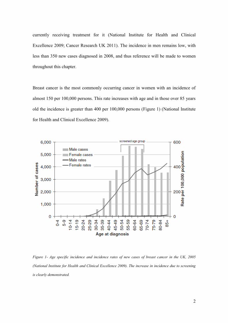
Breast cancer is the most commonly occurring cancer in women with an incidence of
almost 150 per 100,000 persons. This rate increases with age and in those over 85 years
old the incidence is greater than 400 per 100,000 persons (Figure 1) (National Institute
for Health and Clinical Excellence 2009).
Figure 1- Age specific incidence and incidence rates of new cases of breast cancer in the UK, 2005
(National Institute for Health and Clinical Excellence 2009). The increase in incidence due to screening
is clearly demonstrated.

3
The incidence of the disease has risen across all age groups in the UK over the past two
decades (Figure 2). Evidence suggested that this rate of increase may be stabilising
although figures released in 2011 reported that the incidence had risen by 3.8% in the
last decade (Cancer Research UK 2011; National Institute for Health and Clinical
Excellence 2009).
Figure 2- Trend in age specific incidence rates of breast cancer in the UK (National Institute for Health
and Clinical Excellence 2009).
Whilst the incidence rate of breast cancer has been rising over the last 20 years the
mortality rate has been consistently falling since the late 1980s (Figure 3). This may
partly be explained by the UK national screening programme but also by increasingly
effective treatment modalities (National Institute for Health and Clinical Excellence
2009).

4
Figure 3- Age standardised rates of breast cancer mortality in the UK 1971-2005(National Institute for
Health and Clinical Excellence 2009).
These improvements are reflected in the survival rates following diagnosis.
Examination of the relative survival rate, defined as the proportion of patients with a
particular condition who are alive at the end of a set period when compared to similar
people of the same age that do not have the condition, confirms this. In the 1970s the
relative survival rate of patients five years after diagnosis was less than 60%, this
increased to just less than 70% by the 1990s and now stands at 80% for women
diagnosed in the period between 2001-2003 (Early Breast Cancer Trialists'
Collaborative Group (EBCTCG) 2005; NHS Cancer Screening Programmes and West
Midlands Cancer Intelligence Unit 2009; West Midlands Cancer Intelligence Unit,
2009).

5
Closer examination of these survival figures, when categorised according to the stage of
the disease at diagnosis, reveals wide variations. Five year survival for those with stage
I disease (tumour less than 2 cm diameter and no evidence of metastases) is greater than
90%, but for those diagnosed with stage IV disease (evidence of distant metastases) the
survival rate is less than 15% (Figure 4). The importance of early diagnosis can’t be
over emphasised and in relation to prognosis diagnosis of the disease before it has
spread beyond the breast is particularly crucial.
Figure 4- 0-10 year relative survival rates broken down by stage at diagnosis for patients diagnosed
between 1990-4 in the West Midlands Cancer Screening Network (West Midlands Cancer Intelligence
Unit 2009).
The appreciation of the importance of early diagnosis was one of the key influences that
led to the introduction of the national breast screening programme in 1988 (Sant et al.
2006 ). Indeed it is thought that the recent improvements in survival and mortality rates
6
are partly due to advances in treatment for the disease but are largely as a result of the
earlier diagnosis of many patients cancer.
The introduction of the national breast screening programme has meant that women in
the UK with breast cancer present to medical services in one of three ways. This may be
either with a symptomatic lesion, such as a breast lump, or with an asymptomatic
change that was detected by either the screening programme or during an unrelated
investigation. In 2006 just over 30,000 new cases presented with symptomatic changes
and just under 16,000 patients presented via the screening programme (NHS Breast
Screening Programme 2008).
As would be anticipated patients presenting via the screening programme, with an
asymptomatic lesion, had a lower grade of disease than those who presented with a
symptomatic lesion. 83% of patients presenting via screening have disease classified in
the three most favourable prognostic index groups as opposed to 51% who present
symptomatically (Rovera et al. 2008). By definition, this means that the percentage of
patients who have spread of the disease from the breast will be lower in the group of
patients presenting via screening.
This “contemporary” cohort of patients that present via the screening programme have,
on average, a lower grade of disease, which is picked up at an earlier stage, with a
reduction in the presence of disease beyond the breast. This has encouraged the
adoption of new techniques in the surgical management of breast cancer that reduce
both the invasiveness of treatment and the morbidity and psychological effects of

7
surgery. Breast conserving surgery , breast reconstruction and sentinel node biopsy are
all examples of this change. It is hoped that Raman spectroscopy can further
compliment this by allowing for the intra-operative assessment of axillary lymph nodes.
As will be discussed later in the chapter this in turn would allow for an immediate
axillary clearence, if indicated, rather than a delayed second procedure.
1.2. Anatomy, Histology and Pathology of the Human Breast and Lymph
Nodes
The diagnosis and management of breast cancer is based on an appreciation of the
anatomy and pathology of the breast. Therefore prior to discussing the treatment of
breast cancer and reviewing in detail the management of the axilla, the key anatomical,
pathological and histological features of normal and malignant breast tissue will be
reviewed.
1.2.1. The human breast
The adult female breast sits on the anterior wall of the thorax and its base extends from
the second to the sixth rib in the anatomical position. The medial aspect borders the
lateral edge of the sternum and the lateral edge extends to the mid-axillary line. The
axillary tail (of Spence) extends into the axilla along the inferior border of pectoralis
major (Moore 2005) (Figure 5).

8
Figure 5- The anatomy of the female breast (adapted from Ellis 2003).
Histologically the breast can be viewed as a highly modified apocrine sweat gland
which radiates towards the nipple. It is made up of 15-25 independent glandular units
referred to as breast lobes (Wheater, Burkitt and Daniels 1995) (Figure 5, 6).
The lobes are surrounded by adipose tissue and are separated from each other by fibrous
septa. Working from proximal to distal within a lobe there are a number of continuous
structures. At the proximal end is a collection of secretory alveoli. The inner layer of
each alveolus is lined with luminal epithelial cells and is surrounded by both a basal
myoepithelial layer and a basement membrane.

9
Figure 6- The components of the female breast (adapted from Wheater, Burkitt and Daniels 1995).
Between 10 and 100 alveoli make up a lobule and they drain into alveolar ducts that are
lined with epithelial cells and surrounded by a basement membrane. Lobules and the
proximal end of the alveolar ducts are referred to as terminal ductal lobular units
(TDLU) and is the site where the majority of breast cancers originate (Ioachim and
Ratech 2002). A variable number of lobules are found in each lobe of the breast and the
ducts draining each lobule will eventually coalesce to form a lactiferous duct that is
specific for each lobe. This duct opens on to a unique point on the nipple surface
(Raftery 2000). The branching network of lobules and the ducts they drain into are
surrounded by collagenous stroma within which is found blood and lymphatic vessels,
fibroblasts and adipose tissue.

10
Figure 7- The branching network of the human breast as seen after H&E staining at 60x magnification
(adapted from Wheater, Burkitt and Daniels 1995).
The fibroblasts are responsible for producing the supportive capacity of the stroma
referred to as the extra cellular matrix. The stroma found within lobules, the intralobular
stroma, and that found between lobules, the interlobular stroma has different
characteristics. The intralobular stroma contains more fibroblasts and inflammatory
cells yet the connective tissue is more loosely arranged whereas the interlobular stroma
contains far less cells and has more closely packed collagen (Ioachim and Ratech 2002).
11
1.2.2. Histopathology of Breast Cancer
Cancer is defined as a disease in which a group of abnormal cells grow uncontrollably
by disregarding the normal rules of cell division. Cancer may be classified according to
the cells from which the uncontrolled growth originates (Hejmadi 2010).
Carcinoma, a cancer arising from epithelial cells, is the most common malignancy
affecting the breast and can be further sub-classified into in situ or invasive carcinoma.
Further division of the type of tumour is based on its anatomical site within the breast.
1.2.2.1. Carcinoma in situ
Carcinoma in situ (sometimes referred to as a “pre-malignant” condition) is
predominantly detected as areas of micro-calcification on mammography or following
the investigation of an invasive carcinoma. These changes can be defined as either
ductal (DCIS) or the rarer lobular (LCIS) carcinoma in situ dependent on their position
when viewed histologically. They are characterised by a neoplastic growth of the
epithelium that is limited by the basement membrane. It is often associated with
dystrophic calcification around the site and it is this that makes it visible on
mammograms.
Historically this diagnosis was rare as it seldom resulted in overt symptoms. However
since the introduction of screening programmes its incidence has risen and it now
accounts for 22% of all screen detected breast cancers (NHS Cancer Screening

12
Programmes and West Midlands Cancer Intelligence Unit 2009). DCIS maybe
classified as low, medium or high grade dependent on the atypia of the cancerous cells
and this classification is an effective method of predicting the risk of reoccurrence
following excision (National Institute for Health and Clinical Excellence 2009).
A varient of DCIS is atypical ductal hyperplasia (ADH). This is an intraductal
epithelial proliferation that either shows some but not all of the features of DCIS or has
features consistent with DCIS but is only present in a very small area. The presence of
ADH is a risk factor for the development of either DCIS or invasive ductal carcinoma.
As will be discussed in later sections, the assessment of the axillary lymph nodes is not
normally indicated in DCIS. It is therefore very unlikely that many of the patients
recruited to this study will have this condition.
1.2.2.2. Invasive Carcinoma
Invasive carcinoma, in contrast to DCIS, invades into the breast stroma and spreads
locally. It also has the potential to infiltrate the vascular and lymphatic systems and
spread beyond the breast (Johnstone et al. 2002). Classification of invasive carcinoma
may be according to anatomical cell origin (subtype) or histological grade. There are 16
subtypes of invasive breast cancer although some are very rarely encountered (Raftery
2000). These classifications are important as they help guide both initial investigations
and subsequent treatment.

13
Invasive ductal carcinoma represents approximately 75% of all invasive carcinomas.
Histologically it is characterised by malignant epithelial cells that originate in the
alveolar ducts and spread within the fibrous stroma. Invasive lobular carcinoma
accounts for between 10-15% of all cases of invasive breast cancer and arises from
epithelium within the breast lobules. It has a tendency to multifocality with indolent and
progressive characteristics that often result in a worse prognosis than ductal carcinoma
(Rhakha, El-Sayed and Powe 2008). Unlike ductal carcinoma, cancer of lobular origin
is less likely to be associated with calcification of the surrounding stroma and is
therefore more difficult to detect on mammography (Raftery 2000).
There are a variety of other types of tumour. These include mucinous carcinomas which
account for 5% of breast cancers, medullary carcinomas that account for less than 5% of
tumours and tubular cancers that represent between 1 and 2% of all breast tumours.
They each have particular characteristics which are beyond the scope of this review
(Rosen 2001).
Each individual tumour can be classified histologically as well as anatomically. This
helps predict how the tumour will progress based on the cytological and architectural
features of the tumour cells. To maintain standardisation each tumour is categorised by
a pathologist using a validated scoring systems such as the Nottingham Grading System
(Elston and Ellis 1991). This grades the tumour according to the degree of tubular
formation, the nuclear pleomorphism, and the mitotic activity into low (I), intermediate
(II) and high (III) grade groups (Table 1).

14
Degree of Tubule
formation within the tumour
Majority of tumour
Moderate Degree
Little or None
1
2
3
Mitotic Count 0-9 Mitoses/10 high power field (hpf)
10-19 Mitoses/10 hpf
20 or > Mitoses/10 hpf
1
2
3
Nuclear Pleomorphism Small Regular Uniform Cells
Moderate Nuclear Size and Variation
Marked Nuclear Variation
1
2
3
Overall grade Low Grade (I)
Intermediate Grade (II)
High Grade (III)
3-5
6-7
8-9
Table 1: The Nottingham grading scale for breast cancer (Elston and Ellis 1991).
1.2.2.3. Breast Cancer and Metastases
The presence of metastases, the migration of cells from the primary tumour to other
sites around the body, is a key indicator of the prognosis of an individual’s disease. The
most common sites of metastasis in breast cancer are to the regional lymph nodes that
drain the breast. If distant spread occurs then the three most common sites are to bone,
the lungs and the liver. The pathological grading of the tumour and the assessment of
both the local lymph nodes and common sites of distant metastasis is used to stage each
individual patient’s disease. It is a standardised way of documenting the extent of the
disease spread at the time of presentation and is used to predict survival and guide
treatment.

15
The most common staging index used across a range of malignancies is the TNM
system. This categorises the disease based on the tumour itself (T), and the presence of
nodal metastases (N) and distant metastases (M) (Johnson et al. 2004). Other staging
indices which are particular to breast cancer include the widely used Nottingham
Prognostic Index (NPI) (Tables 2, 3). There is a clear association between an increasing
NPI score or TNM stage and worsening 5 year mortality (Figure 8).
Factor Score
Lymph nodes No Metastases
1-3 Positive Nodes
>3 Positive Nodes
1
2
3
Grade Stage I
Stage II
Stage III
1
2
3
Vascular Invasion No
Yes
0
1
Tumour Size
Size in cm Multiplied by 0.2
Table 2: The Nottingham prognostic index (NPI). A score is then calculated for each patient by adding
the lymph node score, the grade score and the vascular invasion score and multiplying them by 0.2 of the
tumour size. (Sabel 2009).
Examination of the 5 years survival figures plotted against the stage of the disease
highlight the prognostic importance of metastatic spread. Patients with a T1 tumour
have a 10% reduced 5 year survival if there are lymph node metastases present and in
the presence of distant metastases the 5 year survival is less than 20% (Figure 8).

16
Stage Features
Primary Tumour (T)
Tx
T0
Tis
T1
T2
T3
T4
Not assessed
No evidence of Primary Tumour
Carcinoma in Situ
Tumour < 2cm in diameter
( <0.1=T1mic, <0.5cm = T1a, <1cm=T1b , rest = T1c)
Tumour 2-5cm in diameter
Tumour >5cm in diameter
Any size with direct spread to chest wall or skin
Lymph Node Status (N)
Nx
N0
N1
N2
N3
Regional nodes cannot be assessed
No metastases
Metastases to mobile ipsilateral nodes
Metastases to fixed ipsilateral nodes
Metastases to ipsilateral internal mammary nodes
Metastases (M)
Mx
M0
M1
Presence of distant metastases cannot be assessed
No distant metastases
Distant metastases (including supraclavicular nodes)
Stage 0= Tis, N0, M0
Stage 1= T1, N0, M0
Stage 2a= T 0/1, N1 or T2, N0 , M0
Stage 2b= T2, N1 or T3, N0. M0
Stage 3a= T3, N1 or T1-3, N2 , M0
Stage 3b= T4, Any N, or Any T, N3 , M0
Stage 4= Any T, Any N, M1
Table 3: The TNM index for staging breast cancer (Sabel, 2009)
Interrogation of the NPI also highlights the importance of the number of involved
axillary lymph nodes. A women with a Grade II, 2 cm invasive tumour with no

17
lymphovascular invasion and no distant metastases (NPI = 3.4) has an anticipated 85%
survival rate at 5 years. This is reduced to 50% if greater than 3 lymph nodes are
positive (NPI = 5.4). As will be discussed later these factors also guide further treatment
of the axilla after axillary surgery.
Figure 8- Percentage 5 year survival according to TNM stage or NPI score (Cancer Research UK 2009).

18
1.3. Lymph Nodes and the Lymphatic System
In the management of breast cancer lymph nodes are vital indicators of the spread of
cancer beyond the breast. Metastasis of the cancer to the lymph nodes is an important
factor in predicting the overall prognosis of an individual’s disease. The status of the
lymph nodes is used to help stage the disease and this helps guide treatment options and
regimes (Rovera et al. 2008; Kurosumi and Takei 2007).
1.3.1. Anatomy of the Lymph Nodes
The lymph nodes are part of the lymphatic system which is divided into lymphoid
tissues, such as the thymus, bone marrow or lymph nodes, and the circulating network
that connects them. The circulatory network consists of permeable lymphatic vessels
and capillaries which extend throughout the body.
Excess interstitial fluid within tissues drains into the lymphatic vessels and is eventually
returned to the cardiovascular circulatory system. During this process the fluid is
filtered through lymph nodes that are found at various positions throughout the body
(Figure 9). Specific lymph nodes are responsible for filtering lymph from specific
organs and regions. Within the lymph node the fluid drained from these specific areas is
exposed to a large number of lymphocytes and other cells of the immune system. If an
antigen is recognised it will trigger a cascade of events both within the lymph node and
subsequently beyond it. Immune response mediators will drain from the lymph nodes to
19
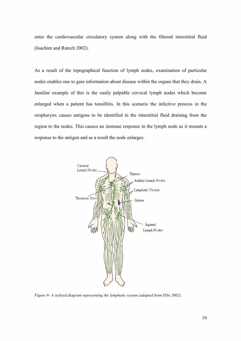
enter the cardiovascular circulatory system along with the filtered interstitial fluid
(Ioachim and Ratech 2002).
As a result of the topographical function of lymph nodes, examination of particular
nodes enables one to gain information about disease within the organs that they drain. A
familiar example of this is the easily palpable cervical lymph nodes which become
enlarged when a patient has tonsillitis. In this scenario the infective process in the
oropharynx causes antigens to be identified in the interstitial fluid draining from the
region to the nodes. This causes an immune response in the lymph node as it mounts a
response to the antigen and as a result the node enlarges.
Figure 9- A stylised diagram representing the lymphatic system (adapted from Ellis 2002).
20
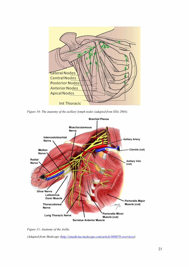
Lymphatic drainage from the breast is primarily to two groups of lymph nodes, the
ipsilateral axillary lymph nodes and the internal thoracic nodes (Figure 10). A small
percentage of lymph will drain to the supra-clavicular and contra-lateral internal
thoracic nodes. Examination of these groups of nodes gives us information about
underlying disease within the breast. Infection, inflammation and importantly in this
study cancer will result in pathological changes within the nodes. These changes may be
determined by clinical examination, radiological imaging or histopathological analysis.
Within the context of this study it is hoped that interrogation of the axillary nodes using
Raman spectroscopy will help determine whether the breast cancer has metastasised to
the lymph nodes.
The axillary nodes are divided according to either their anatomical position or their
relation to surrounding structures. Anatomically they may be defined as lateral, central,
posterior, anterior or apical (Figure 10). Surgically they are more often defined
according to their position in relation to pectoralis minor. They are termed level I if they
are inferior to the pectoralis minor, level II if they are posterior to the pectoralis minor
and level III if they are superior to the pectoralis minor (Ellis 2002). Within the axilla
the lymph nodes lie close to a number of structures including the axillary vein and
artery, the long thoraciac nerve, the thoraco-dorsal nerve and the intercostobrachial
nerve (Figure 11). Careful identification and preservation of these structures, where
possible, helps reduce the morbidity associated with operative dissection of the nodes in
this region.
21
Figure 10- The anatomy of the axillary lymph nodes (adapted from Ellis 2003).
Figure 11- Anatomy of the Axilla
(Adapted from Medscape (http://emedicine.medscape.com/article/880878-overview)).

22
1.3.2. Histology of the Lymph Node
Lymph nodes are bean shaped aggregations of lymphocytic tissue and can vary from a
few millimetres to several centimetres in diameter dependent upon the reactive status of
the node at that time (Figure 12) (Obwegeser et al. 2000).
Figure 12- The structure of an axillary lymph node (adapted from Cacaecu 2008).
Lymph nodes are intrinsically involved in both humoral, involving antibodies, and cell
mediated immunity. Antigens in the afferent lymphatic fluid will be trapped within the
node by either lymphocytes or accessory cells such as dendritic reticular cells, inter-
23
digitating reticular cells or histiocytes. The antigenic cells are then processed and
presented to further lymphocytes which trigger an immune response both locally and
further a field (Ioachim and Ratech, 2002).
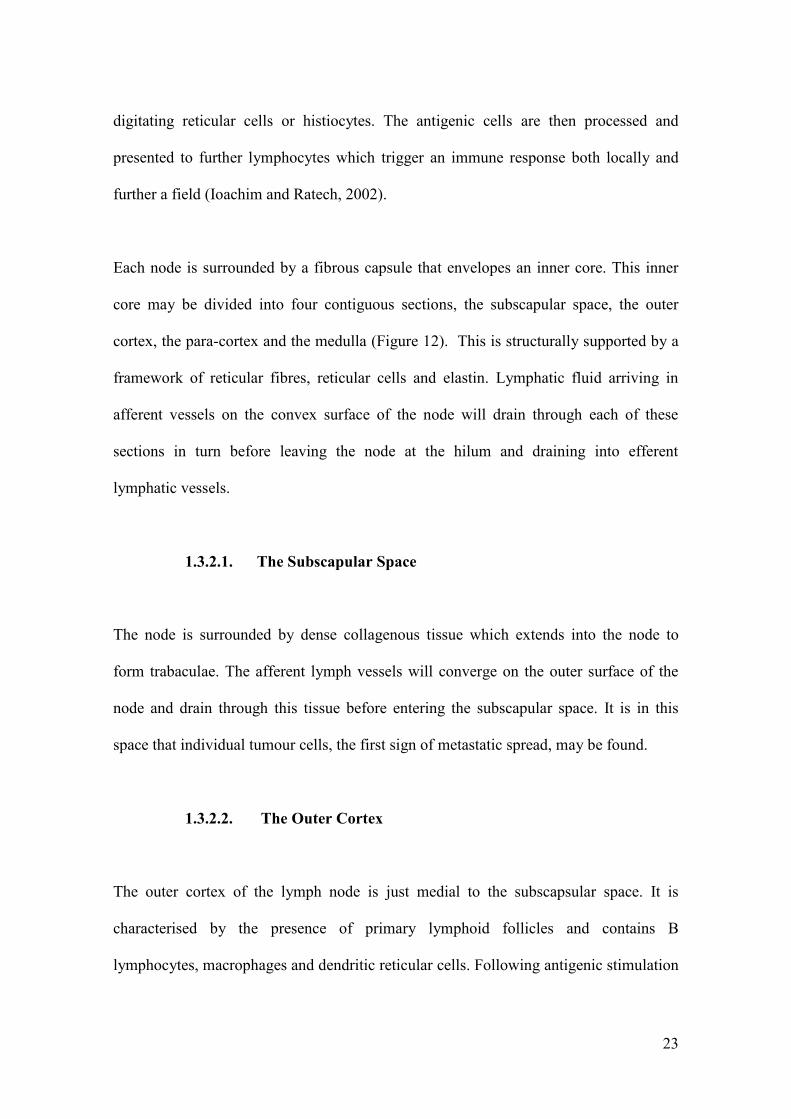
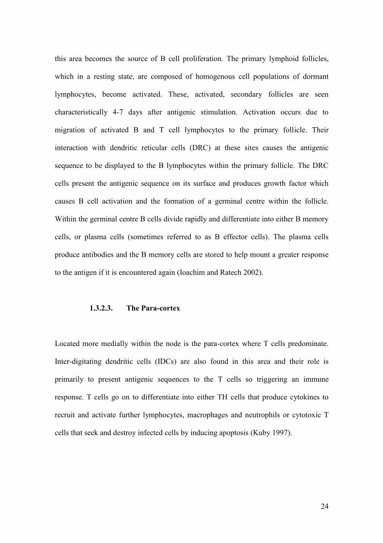
Each node is surrounded by a fibrous capsule that envelopes an inner core. This inner
core may be divided into four contiguous sections, the subscapular space, the outer
cortex, the para-cortex and the medulla (Figure 12). This is structurally supported by a
framework of reticular fibres, reticular cells and elastin. Lymphatic fluid arriving in
afferent vessels on the convex surface of the node will drain through each of these
sections in turn before leaving the node at the hilum and draining into efferent
lymphatic vessels.
1.3.2.1. The Subscapular Space
The node is surrounded by dense collagenous tissue which extends into the node to
form trabaculae. The afferent lymph vessels will converge on the outer surface of the
node and drain through this tissue before entering the subscapular space. It is in this
space that individual tumour cells, the first sign of metastatic spread, may be found.
1.3.2.2. The Outer Cortex
The outer cortex of the lymph node is just medial to the subscapsular space. It is
characterised by the presence of primary lymphoid follicles and contains B
lymphocytes, macrophages and dendritic reticular cells. Following antigenic stimulation
24
this area becomes the source of B cell proliferation. The primary lymphoid follicles,
which in a resting state, are composed of homogenous cell populations of dormant
lymphocytes, become activated. These, activated, secondary follicles are seen
characteristically 4-7 days after antigenic stimulation. Activation occurs due to
migration of activated B and T cell lymphocytes to the primary follicle. Their
interaction with dendritic reticular cells (DRC) at these sites causes the antigenic
sequence to be displayed to the B lymphocytes within the primary follicle. The DRC
cells present the antigenic sequence on its surface and produces growth factor which
causes B cell activation and the formation of a germinal centre within the follicle.
Within the germinal centre B cells divide rapidly and differentiate into either B memory
cells, or plasma cells (sometimes referred to as B effector cells). The plasma cells
produce antibodies and the B memory cells are stored to help mount a greater response
to the antigen if it is encountered again (Ioachim and Ratech 2002).
1.3.2.3. The Para-cortex
Located more medially within the node is the para-cortex where T cells predominate.
Inter-digitating dendritic cells (IDCs) are also found in this area and their role is
primarily to present antigenic sequences to the T cells so triggering an immune
response. T cells go on to differentiate into either TH cells that produce cytokines to
recruit and activate further lymphocytes, macrophages and neutrophils or cytotoxic T
cells that seek and destroy infected cells by inducing apoptosis (Kuby 1997).

25
1.3.2.4. The Medulla
The medulla is the innermost part of the lymph node and is the area most sparsely
populated with lymphocytes. The majority of cells found within the region are plasma
cells that have originated from the germinal centres in the outer cortex. Within the
medullary region they differentiate and produce antibodies. These antibodies leave the
node in the efferent lymphatics and blood vessels and circulate around the body to target
specific matching antigens.
1.3.2.5. Lymph Node Sinuses
The lymphatic fluid drained from individual tissues passes through the different sections
of the node via a series of interconnecting sinuses. These sinuses are lined with
endothelial cells and lymphocytes. Plasma cells and phagocytes can also be found
within the sinus walls. At the cellular level this is an important site for the initial
interaction between the antigens and the cells of the immune system.
The result of this complex filtering network is that the lymph node is able to rapidly
alter both its own cellular components and the composition of the efferent lymphatic
fluid that drain from it. Following immune reactions, in response to both infection and
tumour metastasis, the node becomes enlarged and the concentration of lymphocytes
and antibodies leaving the node is greatly increased. In the context of metastatic spread
this may provide a degree of regional control of cancer cell dissemination. Metastasis to
the lymph node is therefore most often seen prior to distant spread to other organs

26
(Ioachim and Ratech 2002). Within the node itself metastatic cells will first appear in
the subscapular space before progressing through the node to the sinuses, medulla and
cortex. Once established metastatic disease starts to proliferate from the medulla and
eventually the whole node can be over run by self replicating cells (Figure 14).
Figure 14- Histological slide (H and E stained) showing normal lymph node tissue and metastatic breast
cancer in an axillary lymph node (adapted from Wheater, Burkitt and Daniels 1995).
As will be discussed later, these metastatic deposits may be termed isolated tumour
cells, micrometastases or macrometastases. The clinical significance of each of these
differs and will be reviewed later in the chapter. The presence of self-replicating
metastatic cells with the lymph node activates myofibroblasts and cytokines. In turn this
will also stimulate the overgrowth of the surrounding connective tissue which may
result in the formation of scar like tissue around the metastases which is referred to as
desmoplastic change (Ioachim and Ratech 2002).

27
The histological changes seen in positive lymph nodes, when metastatic cells replicate,
reflects the histology of the underlying tumour. There is a correlation of greater than
95% between the tumour seen in the breast and the changes seen within positive axillary
lymph nodes (Ioachim and Ratech 2002). It is argued that if the changes within a
positive lymph node do not match those seen in the underlying tumour then further
examination of the breast tumour should be carried out to ensure that there is not
another primary source.
1.4. Treatment of Breast Cancer
As has been discussed patients may present with breast cancer in one of three ways.
They can present with symptomatic changes, via the national breast screening
programme, or due to an incidental finding when investigating another problem. The
initial role of the team caring for that patient is to confirm the diagnosis, remove the
tumour and then stage the disease. Armed with this information a multi-disciplinary
team will then plan the optimal treatment for each individual.
Confirmation of the diagnosis of breast cancer is made after a triple assessment. This
involves clinical examination, radiological assessment, in the form of a mammogram or
an ultrasound scan, and histopathological review of fine needle aspiration samples or
core needle biopsy samples of the suspicious area. This assessment most often takes
place in secondary care and usually at a one stop clinic. If a diagnosis of invasive breast
cancer is made then initial assessment of the axilla for evidence of metastasis should
also be offered at this early stage (National Institute of Health and Clinical Excellence

28
2009). Further details of the assessment and management of the axilla will be discussed
in subsequent sections.
The management of breast cancer continues to evolve and varies from patient to patient.
In this section a brief overview of the treatment options will be given to help set the
scene for this project although it is recognised that this is not an exhaustive review.
1.4.1. Management of Invasive Breast Cancer
The first procedure in the treatment of invasive cancer is the excision of the primary
tumour with adequate clear margins. If the tumour is locally advanced or there is
evidence of inflammatory breast cancer then a course of neo-adjuvant treatment may be
offered (whereby endocrine therapy or chemotherapy is given as the primary modality
prior to surgery) (National Institute of Health and Clinical Excellence 2009). Surgical
excision may be performed by a number of techniques including breast conserving
methods, such as a wide local excision, or by means of a mastectomy (a surgical
procedure to remove all of the breast tissue) with or without immediate or delayed
breast reconstruction. Assessment of the axillary lymph nodes, if not achieved
preoperatively, is also performed during this initial operation.
Further adjuvant treatment in the form of radiotherapy, chemotherapy or endocrine
medication (such as Tamoxifen, an oestrogen receptor antagonist or Aromatase
Inhibitors, that block production of oestrogen) is offered based on the grade of the
tumour, the stage of the disease and the receptor status of the tumour (Table 4).

29
Nodal
Status
Tumour Type
(See Table 3)
ER + and
HER +
ER + HER + ER /HER -
Normal
Nodes
T1a None
None
None
None
T1b
(well differentiated)
None
None
None None
T1b
( moderate or poorly
differentiated)
Endocrine
+/- Chemo
Endocrine
+/- Chemo
Chemo Chemo
T1c Endocrine
+ Chemo
Endocrine
+ Chemo
Chemo Chemo
T2 or above Endocrine
+ Chemo
Endocrine
+ Chemo
Chemo Chemo
Micro
Metastases
T1a Endocrine
Treatment
Endocrine
Treatment
+/- Chemo +/- Chemo
T1b Endocrine
Treatment
Endocrine
Treatment
+/- Chemo +/- Chemo
Macro
Metastases
Any T Endocrine
+ Chemo
Endocrine
+ Chemo
Chemo Chemo
Table 4- Recommendations for the adjuvant treatment of breast cancer dependent on the tumour type and
the status of the axilla (National Institute for Health and Clinical Excellence 2009). ER= Oestrogen
Receptor, HER = Human epidermal growth factor receptor-2, Chemo=Chemotherapy, Endocrine
Treatment = Tamoxifen or Aromatase Inhibitors.
1.4.2. Management of Ductal Carcinoma in Situ (DCIS)
As previously discussed the management of DCIS has become a significant part of the
breast services remit. Following the introduction of a national breast screening

30
programme up to 1 in 5 cancers detected by screening in the UK are proven to be DCIS
(National Institute for Health and Clinical Excellence 2009). It is expected that
this number will continue to rise with further technological improvements in imaging
and the expansion of the breast screening programme (Patani, Cutuli and Mokbel 2008).
Although classified as a pre invasive condition not all patients will go on to develop
invasive breast cancer following a diagnosis of DCIS. Estimates of the percentages that
will progress to invasive cancer range from 14-75% (Patani, Cutuli and Mokbel 2008).
Progression to invasive cancer is most likely to occur in high grade DCIS especially if
combined with other risk factors such as a palpable mass at presentation, a family
history of breast cancer, wide spread micro-calcifications on mammography and
extensive disease.
Similarly to invasive cancer the management of DCIS starts with the excision of the
affected area. This is most often achieved with breast conserving surgery but if the
tumour is greater than 4 cm, multi-centric or at the site of reoccurrence mastectomy is
the preferred option. Adjuvant radiotherapy to the breast has been shown in a meta-
analysis of randomised controlled trials to reduce the local recurrence by 60% and
should be offered to those patients undergoing breast conserving surgery (Patani , Cutuli
and Mokbel 2008).
The investigation and management of the axilla, in DCIS, is more controversial as by
definition the tumour cells should not have invaded beyond the basement membrane.
However, extensive DCIS may harbour foci of invasive disease and assessment should
be offered to patients with either high grade or widespread disease. A retrospective

31
study of lymph node positive DCIS patients demonstrated that careful examination of
the tumour revealed small foci of invasive disease that had not originally seen.
Therefore lymph node assessment in DCIS is reserved for patients where extensive
disease is present (Sakr et al. 2006). The role of further adjuvant treatment in the form
of tamoxifen has been evaluated in the NSABP-B24 trial and the UK/ANZ DCIS trial
(Sibbering 2009). These studies report minimal reductions in local reoccurrence and
must be balanced against the potential side effects of the treatment.
1.5. The Assessment and Management of the Axillary lymph nodes
The prognostic importance of local metastatic spread to the axillary lymph nodes can
not be over emphasised. Indeed it has consistently been shown to be the most important
marker of prognosis in patients newly diagnosed with breast cancer (Rovera et al. 2008 ;
de Boer et al. 2010). Indeed since the end of the 19th
surgical treatment of breast cancer
included axillary node dissection as standard (Kurosmi and Takei, 2007; Suami et al.
2008).
The method by which axillary node assessment and hence staging is carried out has
altered over time, reflecting the move to increasingly less extensive surgical techniques.
Like assessment of the breast, axillary lymph nodes may be examined clinically,
radiologically or by histopathological methods. In this section the current methods by
which axillary nodes are sampled and assessed will be reviewed. Current controversies
in this area will then be discussed and the potential clinical role that Raman
spectroscopy could play in lymph node assessment in the future will be highlighted.

32
1.5.1. Lymph node assessment
Initial attempts at lymph node assessment should take place after the diagnosis of breast
cancer is made. It is recommended that all patients newly diagnosed with invasive
disease undergo ultrasound examination of the axilla with guided biopsy of areas of
suspicion prior to their initial surgery (National Institute of Health and Clinical
Excellence 2009). The reported sensitivity (its ability to identify true positives) and
specificity (its ability to identify true negatives) of ultrasound scans (USS) at detecting
metastatic spread depends on the criterion of positivity (Alvarez et al. 2006). When
lymph node size is used the sensitivity is between 66 and 73% and the specificity is
between 44 and 98%. If morphological characteristics of the node are used then the
reported sensitivity ranges from 55 to 92% and the specificity from 80 to 97% (Alvarez
et al. 2006). The recommended technique is USS of the axilla and either FNA (fine
needle aspirate) or core biopsy if there are abnormal morphological features. Sensitivity
for this approach varies between 31 and 63% with reported specificities of 100%
(Damera et al. 2003 ; Alvarez et al. 2006). Factors that influence the success of this
technique are the experience of the radiologist, the imaging and biopsy equipment and
the number of aspiration or biopsy samples taken (Damera et al. 2003).
If the nodes are found to be positive then the patient is recommended to have an axillary
dissection most often at the same time as surgery to excise the tumour in the breast. Due
to the low sensitivities of this technique patients with a negative USS still require
further evaluation of their axilla.

33
The use of preoperative positive emission tomography (PET) for staging the axilla has
also been investigated. However a recent systematic review and meta-analysis reported
wide variations in both sensitivity (20-100%) and specificity (75-100%). Given these
results along with the costs and resource implications the authors concluded that the
technique should not replace USS as a pre-operative method of evaluating the axilla
(Cooper et al. 2011).
The traditional method of axillary node sampling, which took place as part of the
operation to remove the breast tumour, involved dissection of the tissue in the axilla,
referred to as axillary node dissection (ALND). Between 15 and 20 nodes were excised
along with the tissue in that area (Steele et al. 1985; Mansel et al. 2006). An alternative
approach was 4 node sampling followed by radiotherapy if they were found to be
positive (Steele et al. 1985).
Axillary sampling using these methods carried significant co-morbidities including
nerve injury, resulting in parasthesia of parts of the ipsilateral arm, lymphoedema and
shoulder stiffness (Mansel et al. 2006). With the emergence of breast conserving
surgery in the 1980s focus shifted to developing surgical techniques that reduced the
invasiveness of axillary sampling and reduced the risks to the patient. The onset of
breast screening programmes and hence the earlier stage of breast cancer at presentation
added impetus to this goal.
34
1.5.2. Sentinel Lymph Node Biopsy (SLNB)
The last decade has seen the emergence of SLNB as the standard of care for the
sampling of the axillary lymph nodes. The technique was developed on the principle
that cancer cells that have invaded lymphatic vessels draining the breast will initially
reach specific (sentinel) lymph nodes.
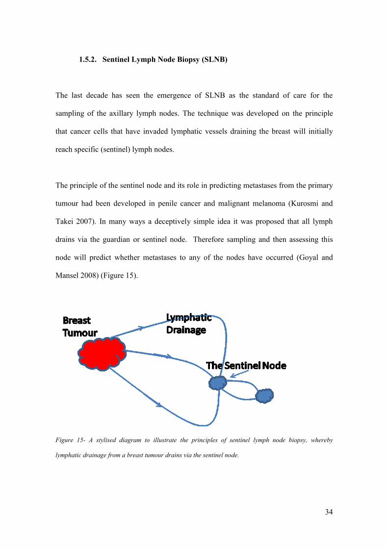
The principle of the sentinel node and its role in predicting metastases from the primary
tumour had been developed in penile cancer and malignant melanoma (Kurosmi and
Takei 2007). In many ways a deceptively simple idea it was proposed that all lymph
drains via the guardian or sentinel node. Therefore sampling and then assessing this
node will predict whether metastases to any of the nodes have occurred (Goyal and
Mansel 2008) (Figure 15).
Figure 15- A stylised diagram to illustrate the principles of sentinel lymph node biopsy, whereby
lymphatic drainage from a breast tumour drains via the sentinel node.
35
The status of the sentinel node has been demonstrated to reflect the overall status of the
axilla in 97% of cases (Layfield et al. 2011). If the sentinel nodes are negative then the
axilla is deemed clear of metastases and the rest of the nodes need not be dissected. This
has been shown to reduce the morbidity and complications associated with traditional
methods of node sampling (Mansel et al. 2006).
The technique of SLNB was first described in breast cancer in the early 90s (Krag et al.
1993; Giuliano et al. 1994). Since then a number of case series and randomised control
trials have been published documenting its use. A meta-analysis of 69 studies published
in 2006 pooled data from more than 8000 patients and concluded that the technique was
successful at identifying the sentinel node in 95% of cases and had a false negative rate
of less than 7% (Kim et al. 2006). These results, combined with the marked reduction in
morbidity has meant that SLNB has now been adopted as the standard for the initial
sampling of the axillary lymph nodes and is being used more and more widely
throughout the UK (National Institute for Health and Clinical Excellence 2009). It is
well accepted by patients due to its lower risks and the shorter associated hospital stay
(Purushotham et al. 2005).
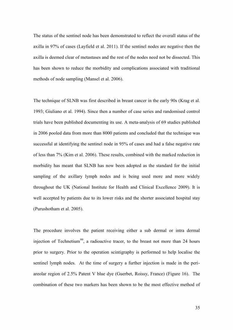
The procedure involves the patient receiving either a sub dermal or intra dermal
injection of Technetium99
, a radioactive tracer, to the breast not more than 24 hours
prior to surgery. Prior to the operation scintigraphy is performed to help localise the
sentinel lymph nodes. At the time of surgery a further injection is made in the peri-
areolar region of 2.5% Patent V blue dye (Guerbet, Roissy, France) (Figure 16). The
combination of these two markers has been shown to be the most effective method of

36
correctly identifying the sentinel lymph node (Goyal and Mansel 2008). During the
procedure the lymph node position is confirmed using a hand held gamma probe. A
small incision is then made over the site and the node is identified visually before being
excised.
Figure 16- An intra operative photograph of an axillary lymph node (arrow) stained blue identified
during a sentinel lymph node biopsy (Authors own copy).
1.5.3. Histopathological Assessment of Axillary Nodes
The presence of metastatic spread within an axillary node may be defined as either
macrometastases, cell masses greater than 2 mm in diameter, micrometastases, cell
masses between 0.2 and 2 mm in diameter or isolated tumour cells, single cells or
clusters of cells less than 0.2 mm in diameter.
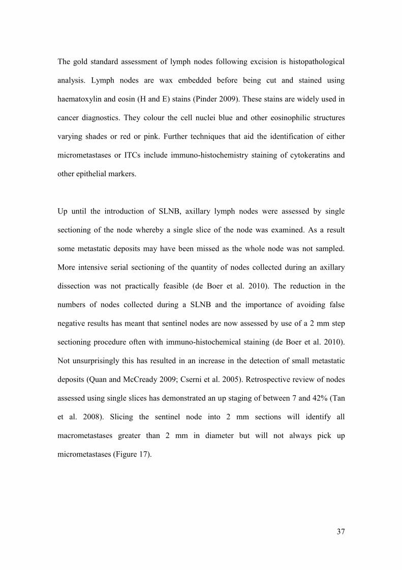
37
The gold standard assessment of lymph nodes following excision is histopathological
analysis. Lymph nodes are wax embedded before being cut and stained using
haematoxylin and eosin (H and E) stains (Pinder 2009). These stains are widely used in
cancer diagnostics. They colour the cell nuclei blue and other eosinophilic structures
varying shades or red or pink. Further techniques that aid the identification of either
micrometastases or ITCs include immuno-histochemistry staining of cytokeratins and
other epithelial markers.
Up until the introduction of SLNB, axillary lymph nodes were assessed by single
sectioning of the node whereby a single slice of the node was examined. As a result
some metastatic deposits may have been missed as the whole node was not sampled.
More intensive serial sectioning of the quantity of nodes collected during an axillary
dissection was not practically feasible (de Boer et al. 2010). The reduction in the
numbers of nodes collected during a SLNB and the importance of avoiding false
negative results has meant that sentinel nodes are now assessed by use of a 2 mm step
sectioning procedure often with immuno-histochemical staining (de Boer et al. 2010).
Not unsurprisingly this has resulted in an increase in the detection of small metastatic
deposits (Quan and McCready 2009; Cserni et al. 2005). Retrospective review of nodes
assessed using single slices has demonstrated an up staging of between 7 and 42% (Tan
et al. 2008). Slicing the sentinel node into 2 mm sections will identify all
macrometastases greater than 2 mm in diameter but will not always pick up
micrometastases (Figure 17).

38
Whilst it is recognised that this technique may miss some micrometastases it is designed
to ensure that all macrometastases are detected. More extensive techniques that have a
greater sensitivity for micrometastases have been described. The implications these
have on resources has meant that they are unlikely to be fully implemented as the low
clinical significance of micrometastases and isolated tumour cells (ITCs) becomes more
fully understood (Veronesi et al. 2001). New techniques, such as Raman spectroscopy,
may therefore have an advantage over standard histopathology as more of the node will
be sampled without the associated increased resource requirement.
Figure 17- An illustration of the importance of sectioning a lymph node to demonstrate how micro-
metastases could be missed.

39
Before the introduction of SLNB all lymph nodes with metastatic deposits of < 2 mm in
diameter were classified as lymph node positive micrometastases (de Boer et al. 2010).
However current UK guidelines state that the presence of either macro or
micrometastases renders the lymph node positive for metastatic spread but nodes with
purely isolated tumour cells are regarded as negative (Pinder 2009).
1.5.4. Management of the positive axilla
The further management of the axilla once positive nodes have been detected depends
on the method by which the metastases were detected. A summary based on current
NICE guidelines is shown in Figure 18.
Figure 18- A flow chart demonstrating the management of the axilla in breast cancer.
40
If there is evidence of metastases from the primary tumour in the SLN then it is
recommended that the patient undergoes an axillary dissection to remove all of the
lymph nodes in the region (National Institute for Health and Clincal Excellence 2009).
Until recently it has been argued that this was necessary for complete staging, improved
loco-regional control and perceived improvement in overall survival (Giuliano et al.
2010). It is also worth noting that the current NICE guidelines suggest that all node
positive patients receive docetaxal chemotherapy as part of an adjuvant chemotherapy
regimen. This is important as a false positive node assessment will result in the patient
undergoing both an unnecessary axillary dissection, and if there is no opportunity for
post operative result confirmation, a course of chemotherapy (National Institute for
Health and Clinical Excellence 2009).
Data from the recently published ACOSOG-Z0011 trial has ignited discussion in this
area and questioned our current management of patients with positive lymph nodes. It
will be discussed further in subsequent sections (Giuliano et al. 2010).
1.5.5. Intra-operative Assessment of Sentinel Lymph Nodes
Standard post operative assessment of axillary lymph nodes sampled during a SLNB
necessitates the need for a second surgical procedure, an axillary lymph node dissection
(ALND), at a later date if the sentinel node is positive. Given that 25-30% of patients
undergoing a SLNB will have positive nodes a method of intraoperative nodal (IO)
assessment has been actively sought (Layfield et al. 2011).
41
There would be advantages to IO assessment for the patient, the surgeon and the health
care system. It has been reported that the delay whilst waiting for results and the effect
of requiring a further operation adds to the psychological stress the patient experiences,
and a methodology of immediate nodal assessment and ALND, if required, is favoured
by patients (Chicken, Sivanadarajah and Keshtgar 2007). Economic analysis carried out
in the UK supports the use of intra-operative testing with estimated savings of up to
£1000 per patient receiving immediate ALND (Burke and Setters 2010). It has also
been argued that further surgery delays the onset of adjuvant treatment which may have
an impact on long term outcomes (Snook et al. 2011).
Despite these advantages caution has been expressed because of questions about the true
economic benefits of IO assessment, the psychological effect on the patient and the true
prognostic role of SLNB detected metastases. It has been argued that the number of
patients who could benefit from intra-operative analysis is less than that used in the
economic analysis of intra-operative testing (Benson and Wishart 2010). Despite 25-
30% of patients having positive nodes data from our own unit suggest that less than
10% of these will return to theatre purely for an ALND (10/121 patients over a 12
month period) (Horsnell et al. 2012). The re-excision of tumour margins, or more
significant breast surgery such as a completion mastectomy or breast reconstruction all
require second operations during which time an ALND could be performed. Further to
this the psychological impact of patients finding out in the recovery room that they have
positive nodes by discovering an axillary drain in situ (necessary because of the
increased invasiveness of the surgery) has also not been fully explored and will require

42
careful explanation by the operating surgeon prior to the surgery (Benson and Wishart
2010).
Despite this support has grown for an effective method of intra operative node
assessment and has been endorsed by the NHS Technology Adoption Centre (NTAC).
The ideal technique in this setting would therefore need to be both sensitive and specific
in comparison to the gold standard, quick and user friendly within the theatre setting,
economically viable and operable without significant added expertise.
There are currently 3 established techniques for the intra-operative assessment of
axillary lymph nodes, frozen section analysis, imprint cytology and molecular assays.
Each of these techniques has a number of disadvantages and thus despite the evident
potential benefits their use varies. A pan-European survey published in 2004 reported
that of the 240 units that responded to the authors, only 60% used some form of intra-
operative assessment (Layfield et al. 2011).
1.5.5.1. Frozen Section Analysis
Frozen section analysis is a well established technique that is familiar to all
pathologists. It is used in a number of clinical situations where the information derived
will be used to guide the patient’s immediate management. Current intra operative uses
include the differentiation of malignant and benign causes of a frozen pelvis, the
identification of resection margins in abdomino-perineal resections or the confirmation
of tissue type in parathyroidectomy. Although widely used it has a number of
43
disadvantages. These include the effect of freezing artefact, the processing time and the
need to have immediate access to both an experienced histopathologist and a skilled
biomedical scientist (Keshtgar 2009). The sensitivity of this procedure compared to the
gold standard, post operative analysis, has been reported as 57-76%, although the
specificity is consistently reported as approaching 100% (Creager and Geisinger 2002;
Chao 2004; Layfield et al. 2011). Methods of altering the technique to increase the
sensitivity have been suggested including multi serial sectioning or the use of rapid
immunohistochemistry (IHC) stains (Veronesi et al. 2001). The added workload that
this would entail is not thought to be feasible within the UK health care setting
(Keshtgar 2009).
1.5.5.2. Touch Imprint Cytology
Touch imprint cytology (TIC) is a simple and rapid method of preparing a cytological
specimen for analysis. The excised lymph node is bisected and the cut surfaces are
pressed onto a slide which is then fixed and stained. As a result there is no requirement
for specialised equipment and there is no loss of tissue that would compromise the gold
standard examination of paraffin embedded sections. There does however remain the
need for an experienced histopathologist to interpret the slides that have been created
(Keshtgar 2009). A meta-analysis of 31 studies where TIC had been used to assess the
axillary lymph nodes reported a pooled sensitivity of 63% and a specificity of 99%.
This sensitivity was improved to 82% if the presence of micro-metastases were
excluded. The authors of the meta-analysis estimated that if all the patients whose nodes
were included in the pooled studies had received intra operative TIC node assessment

44
then over 20% would have proceeded to a primary rather than an interval axillary
clearance (Tew et al. 2005). One of the problems with interpreting the results of these
studies has been the heterogenity of the sampling techniques used. In the four studies
reviewed by Layfield variations in technique occurred in all four centres. However the
pooled sensitivity of 63%, which is below that of frozen section, and the added
expertise required accounts for why the technique is less widely used than frozen
section analysis (Layfield et al. 2011).
1.5.5.3. Molecular Assays
Recently molecular assays using either reverse transcriptase polymerase chain reactions
(RT-PCR) or reverse transcriptase loop-mediated isothermal amplifications (RT-
LAMP) have been developed to detect metastasis by quantitatively measuring the
concentration of tumour specific mRNA markers. The two markers CK-19 (used in both
techniques) and mammaglobin (used in the RT-PCR only) are expressed at high levels
in cells of breast origin but are absent or a low level in normal axillary nodes. Studies
analysing the efficacy of these methods to differentiate between positive and negative
nodes have reported sensitivities of between 88 and 98% and specificities of greater
than 93% for the RT-PCR technique (Blumencranz et al. 2007; Tafe 2010). An
unpublished meta-analysis of 8 similarly run studies carried out within our group,
which included a total of 1547 patients, revealed a sensitivity of 88% and a specificity
of 95%.

45
Sensitivities of 95% and specificities of up to 97% have been reported with the RT-
LAMP technique (Tamaki et al. 2009; Visser et al. 2008). A four centre study that
included 204 patients within the UK using OSNA (the commercially available RT-
LAMP equipment) has recently published data with a sensitivity of 91.7% and a
specificity of 96.9% (Snook et al. 2011).
The advantages of these molecular assays include the ability to perform the test without
the need for a specialised histopathologist to interpret the results and in a time frame
that does not delay the surgical procedure. Disadvantages include the need to
homogenise the node which prevents subsequent gold standard histopathological
analysis. This is a particular danger as the false positives would mean that the patient is
condemned to both an unnecessary axillary clearance and a course of chemotherapy as
previously highlighted. It is worth noting that GeneSearch ® (Veridex, LLC, Warren
NJ, and USA) the first commercially available product to exploit the RT-PCR technique
has recently been withdrawn from the market. The high set up costs, logistical
difficulties and the level of false positives were all cited for the low demand that
prompted its withdrawal from the market (Loftus 2010).
1.6. Controversies
It has always been clear that the status of the axillary lymph nodes in breast cancer is
crucial for staging and prognostic prediction. Techniques to both sample and assess
these nodes have changed, particularly since the introduction of sentinel lymph node
biopsy. However in the modern breast screening era patients are often presenting at an
46
earlier stage and this has caused many to re-examine the clinical significance of the
axillary nodes and the need for an ALND if the nodes are found to be positive. This
project is based on the perceived clinical need for a new method of intra-operative
lymph node assessment that would allow immediate ALND to take place if required.
Therefore an understanding of the nature of the ongoing debate is crucial to appreciate
the implications it may have for the future applicability of this research.
1.6.1. What is the significance of positive nodes?
As has been discussed the increased thoroughness of pathological assessment now
applied to sentinel lymph nodes has resulted in up to 40% of nodes being “upstaged”.
Clinicians have therefore asked whether the clinical significance of these positive nodes,
particularly micrometastases and isolated tumour cells (ITCs), is the same as the
traditional H&E single sliced positive nodes on which their long held prognostic
importance is based.
Initially the focus of this debate had been the implication of finding micrometastases
and isolated tumour cells. A recent meta-analysis examined 12 cohort studies
comparing the 10 year outcomes of patients with single sliced H&E positive nodes
(micrometastases and ITCs) against those with negative nodes. This confirmed the
traditional view that patients had a poorer disease free survival rate and overall survival
at 10 years if micrometastases or ITCs were present on the single slice (de Boer et al.
2010).

47
This survival difference was less clear in studies that compared an “occult” group of
positive nodes (where retrospective pathological assessment of single sliced H&E
negative nodes had subsequently identified micrometastases or ITCs) with nodes that
remained negative after step sectioning. Overall survival was not reduced in 3 out of 6
studies that used multivariable analysis and disease free survival was not significantly
different in eight out of 12 studies that recorded this outcome (de Boer et al. 2010).
Analysis of data published since the advent of SLNB was more difficult as relevant
studies were “hampered by small numbers, short follow-up and lack of multi variable
analysis”. The authors went on to include some of the earlier studies that had included a
sub population of patients who underwent SLNB and this suggested a lower disease free
survival and overall survival if metastases of less than 2 mm were present (de Boer et al.
2010). This finding is supported by a retrospective cohort study of more than 2500
Dutch women who had a SLNB. Even after adjustment for diagnosis, tumour grade,
hormone receptor status and ALND there was an increased risk of events among
patients with either micrometastases (hazard ratio 1.56 (95% CI 1.15 to 2.13)) or ITCs
(hazard ratio 1.5 (95% CI 1.15 to 1.94)) as compared to node negative women (de Boer
et al. 2009) (Figure 19). This increased risk was reduced if patients who had
micrometastases or isolated tumour cells received systemic adjuvant therapy.

48
Figure 19- Disease free survival curves over 5 years after diagnosis in patients who are node negative or
who have ITCs and micrometastases (a.) with and without adjuvant treatment (b.) This demonstrates the
worse outcome in patients who had nodal metastases and how this could be mitigated with adjuvant
treatment (adapted from de Boer et al. 2009).

49
This is important as critics of the retrospective studies argue that much of this data is
based on old cohorts of patients who were identified pre-screening programmes and
who did not receive adjuvant treatments. A more contemporary American cohort study
suggested that there was no added benefit for patients with micrometastases who
underwent an ALND after a SLNB in either preventing axillary reoccurrence or overall
survival (Bilimoria et al. 2009). Both the local reoccurrence and the overall survival
were no different if the patient underwent an ALND or not (disease free survival 98% v
99% at 5 years in ITCs and 90 v 89% at 5 years in micrometastases in the no ALND v
ALND groups). This study further went on to show a marked reduction in numbers of
patients having SLND if there was evidence of micrometastases or ITCs in the period
2000 -2005.
Two recent studies that have addressed the question prospectively were the American
College of Surgeons Oncology Group Z-0010 trial and the National Surgical Adjuvant
Breast and Bowel Project (NSABP) - 32 trial. The Z-0010 trial included patients whose
clinicians were blinded to the results of immuno-histochemistry and treatment thus
relied on the single cut H and E slide. This showed that the 5 year overall survival rates
were 95.8% ,in the IHC negative, group as compared to 95.1% in the IHC positive
group (Cote et al. 2010). The NSABP-32 trial showed a slight improvement in survival
in the IHC negative group (95.8% 5 year disease free survival v 94.6%) (Weaver et al.
2011). The differences remain small and thus the role of these “extra” metastases
detected by immuno-histochemistry remains questionable.

50
Added to this debate are studies that support the concept of ITCs being found in a node
for benign reasons. It has been argued that they may be a result of previous
manipulation and instrumentation of the breast tumour. Both fine needle aspiration
(FNA) and core needle biopsy may displace epithelial cells and either benign or
malignant cells have been found in the granulation tissue along the site of the biopsy.
Part of the healing process after these procedures involves interstitial fluid draining to
the axillary lymph nodes. In this way cells of epithelial type may be transported to the
node as a result of a natural healing reaction. Comparison of the cell type may help to
clarify this. If the ITCs are different to the primary tumour it is unlikely to be related to
the tumour. Further if there is evidence of the debris from tissue trauma such as red
blood cells or haemosiderin deposits within the node then a traumatic cause is more
likely (Carter et al. 2000 ; Bleiweiss, Nagi and Jaffer 2006).
These studies support the current UK guidelines that nodes with ITCs are deemed to be
negative. Within these guidelines the presence of micrometastases, as has been
discussed, renders the node positive currently. Based on the studies above this remains a
very controversial area and the benefits of further treatment may be questioned. The
importance of the MDT in discussing the risks and potential benefits of further
treatment in individual patients with these findings is clearly crucial. Thus the place for
immediate ALND, following intra-operative diagnosis, prior to MDT discussion in
these patients may be questioned.
Until recently the position of macrometastases was much more straightforward. The
most recent contribution to the debate has been the results of the Z-OO11 trial (Giuliano
51
et al. 2011). This was a prospective randomised trial of SLNB and no further axillary
treatment versus SLNB and ALND for patients with T1 or T2 tumours and either micro
or macrometastases discovered on H&E slides, who were undergoing breast conserving
treatment and adjuvant therapy. There were a number of exclusion criteria that included
palpable nodal disease, extra nodal spread and more than 3 nodes affected. The results
of this study have shown, at a median follow up of 6.3 years, that there were no
statistically significant differences in either local or regional recurrence amongst the two
treatment groups. The authors suggested a number of possible reasons for this result.
Firstly that SLNB removed the nodes with metastatic spread, stating that in 40-60% of
cases the sentinel node is the only positive node. Secondly they proposed that not the
entire metastatic load in axillary nodes has the ability to develop into clinically
significant disease. As a result of this study they suggest that we may be over treating
the positive axilla. They do sound a note of caution by explaining that this is only
relevant to patients with T1/T2 tumours, undergoing breast conserving surgery with no
clinically palpable axillary disease and less than 3 positive nodes. They also concede
that all the patients in the study underwent opposing tangential field whole breast
irradiation which may well have treated the axilla. Further to this 96% of patients
received systemic adjuvant therapy which may confound the results. However as a
result of these findings the lead author has suggested that the role of ALND needs to be
re-examined and may in the future be eliminated as a requirement for most women with
“contemporary” breast cancer.
The latest National Comprehensive Cancer Network guidelines for the management of
invasive cancer have thus included a category of patients that meet the criteria for the Z-
52
0011 trial and should be “considered” for no further axillary surgery (National
Comprehensive Cancer Network 2012). Despite the finding of the Z0011 trial, SLNB
remains the standard of care for breast cancer patients in the UK and completion ALND
is still recommended if there are macro- or micro-metastases within an axillary lymph
node. Practice is changing and for the management of micro-metastases the place of
ALND is now questioned and thus the role of intra-operative node analysis will be
limited if there is no plan to proceed to an ALND. For macrometastases there remains a
clear place for ALND even if it is in a smaller group of patients in the post Z-0011 era.
This is clearly an issue which will continue to be debated and the results of a number of
ongoing trials will help shape the debate. Trials that look at the outcome of axillary
node dissection versus no axillary node dissection in patients positive for
micrometastases (IBCSG 23-01 Trial) and that assess whether axillary dissection or
axillary radiotherapy is the best treatment option for patients with metastatic spread
(AMAROS (After mapping of the axilla: Radiotherapy or Surgery) Trial) may add
greater pressure onto the advocates of ALND. The results of these trials will be keenly
followed and help shape future management of node positive breast cancer.
As the management of breast cancer continues to progress new methods of prognostic
assessment may also influence the future management strategies. OncotypeDX
(Genomic Health Inc) is a multi gene diagnostic assay based on the gene expression of a
tumour specimen. It is currently being marketed to quantitatively predict the likelihood
of chemotherapy benefits and distant reoccurrence. Based on the level of expression of
16 genes patients can be stratified into one of three groups. This allows patients to make
decisions based on the risk benefit ratio for each sub group, rather than the population

53
as a whole. As a result those patients who would receive the maximum benefit of
systemic treatments can be identified and given the treatment whilst those who would
receive minimal benefits could decide against it due to the side effects and toxicity of
the treatment. (Paik et al. 2006). Studies to date suggest that these techniques may also
be able improve upon standard staging although questions remain with regard to their
efficacy at predicting local reoccurrence and their use for rarer sub types (Gelmon
2010).
1.7. Conclusions
Breast cancer remains a significant cause of morbidity and mortality. It is a disease
which attracts a great deal of clinical research, of which this Raman based study, is one
such example. As a result, the management of the disease will continue to change to
embrace new technologies and techniques. It is of the authors’ opinion that ALND will
continue to retain a place in the management of breast cancer, particularly for patients
with nodes positive for macrometastases that fall outside the criteria of the Z-0011 trial.
As has been demonstrated in this chapter, determining the nodal status of each patient’s
axilla remains important both to guide treatment and to achieve the very best clinical
outcome.
There are pathological differences that exist between a normal axillary lymph node and
one in which metastatic spread has occurred. It is these differences which are exploited
by current techniques. As has been discussed they all have their own advantages and
disadvantages and have not been universally implemented. As a result there remains a

54
need for a technique that can provide patients with the benefits of intra-operative
axillary node testing, in a cost effective way that could be made available to all. It is
hoped that within this study, and thus this thesis, that the potential role of Raman
spectroscopy to fill this void will be established. To achieve this experiments performed
at a preparatory stage, prior to use within an operating theatre, will be reported before
focusing on experiments that were carried out within an operating theatre using fresh
tissue, to establish the technique as one that could be used in a real life clinical setting.

55
2. Raman Spectroscopy and Clinical Diagnostics.
As concluded at the end of the first chapter the aim of this project is to determine
whether Raman spectroscopy could be used as a means of assessing axillary lymph
nodes intra operatively in patients newly diagnosed with breast cancer. In this chapter
the technique and concepts underpinning the use of Raman spectroscopy will be
introduced. Evidence supporting its use in this project will be discussed and supported
by reviewing previously published work.
2.1. The Ideal Diagnostic Tool.
When considering the development of a new diagnostic tool it is important to first
highlight what features would constitute the ideal tool for the scenario in which it is to
be used. As previously discussed in Chapter 1 there are a number of techniques that are
already being used to assess lymph nodes intra-operatively. They all have significant
disadvantages which have prevented their universal use. Analysis of these techniques
suggests the key parameters which a new diagnostic tool entering this environment must
meet.
Firstly and most importantly the tool must be both sensitive (its ability to detect true
positives) and specific (its ability to detect true negatives) in comparison with the gold
standard histopathology assessment. The clinical consequences of a false positive result
would see a patient undergoing an ultimately unnecessary axillary node dissection and
adjuvant chemotherapy. The consequences of a false negative result whilst being less

56
severe would mean that a patient with a positive node was under-staged and potentially
under treated. This can partially be mitigated for by the ability to post-operatively cross
check the tests results. This would however mean that a false negative patient needed a
second operation and thus negate the very benefit it could provide.
Secondly the diagnostic tool must be able to produce a result without unnecessarily
disrupting or delaying the ongoing procedure. It is the author’s opinion that the best way
to achieve this is for the equipment to be used within the operating theatre. This would
reduce the added costs of having separate staff, particularly pathologists, to operate the
device outside theatre and help prevent time delays as well as reducing the risk of tissue
loss whilst transporting the node to an alternative venue. For the device to be used
within theatres it needs to be safe, unaffected by the theatre surroundings and simple to
use. It should be the aim that theatre staff can easily produce a result without significant
added expertise, either in tissue preparation or diagnostic interpretation.
Finally in the current economic environment it is important that the tool is cost
effective. Raman spectroscopy, unlike the other intra-operative methods, has the
potential to fulfil these criteria and this will be demonstrated in this project (Table 5).

57
Frozen Section
Analysis
Touch Imprint
Cytology
Molecular
Assays
Raman
Spectroscopy
Sensitive
To be
determined
Specific
To be
determined
Post Operative
Cross Check
Use within theatre
To be
determined
Time Frame
To be
determined
Cost Effective
To be
determined
Table 5- The features of an ideal diagnostic tool for intra-operative lymph node assessment. For
illustrative purposes the strengths and weakness of current intra-operative techniques are shown, along
with the areas that need to be determined for Raman spectroscopy (further details of the non-Raman
spectroscopy techniques can be found in Chapter 1).
2.2. Raman Spectroscopy - An Introduction
Raman Spectroscopy is based on the inelastic scattering of monochromatic light as it
interacts with molecules. This interaction between light and molecules was first
observed by C.V. Raman in 1928. It is one of a number of interactions that may occur
when light interacts with matter. Light may be reflected, absorbed or as in the Raman
effect, scattered. Each of these modalities may be harnessed to assess matter. To

58
appreciate these interactions we need to consider that light is a form of electromagnetic
radiation and may further be conceptualised as small packets of energy or photons that
exhibit wave particle duality. The relationship between the energy (E) of a photon of
light and its wave frequency (v) is given by the equation;
E=hv
Where h is Planck’s constant (6.63 x 10⁻³⁴
J/s molecule-1
)
The frequency is related to the wavelength (λ) of light by the equation;
v = c / λ
Where c is the velocity of light (2.998 x 10⁸ms
-1)
It is thus apparent that that the energy of a photon of light is inversely proportional to its
wavelength.
The majority of scattering interactions are elastic in nature. In this scenario a photon of
light interacts with a molecule and causes polarisation of its electron cloud and a rise in
its energy state. This new “virtual” energy state is very short lived (approximately 10-14
secs.) after which the molecule returns to its initial energy state. As it returns to its
initial energy state it releases a photon with the same energy and hence wavelength as
the incident light.

59
In contrast Raman scattering is an inelastic interaction. The incident and emitted photon
have different energies and therefore different wavelengths. This occurs because the
molecule, having been excited to a virtual energy state from its initial state, does not
return to the initial energy state but to a higher (or lower) energy state. Therefore the
photon emitted will have an energy which is lower (or higher) than the incident photon.
When the emitted photon has a lower energy it is termed Stokes Raman Scatter and
when the emitted photon has a higher energy it is termed anti-Stokes Raman Scatter.
Many times less than 1% of scattered photons have undergone Stokes Raman scattering,
with even less undergoing anti-Stokes Raman scattering (Figure 20).
Figure 20- The characteristics of Rayleigh, Stokes and Anti-Stokes light scattering, demonstrating that in
Rayleigh scattering the energy level returns to the original state and thus the wavelength of the emitted
light is the same as the incident light that caused the temporary energy level shift. In contrast in Raman
(Stokes and anti-Stokes) the energy level does not return to the original state and thus emitted light has a
different wavelength to the incident light.

60
Within each molecule there are defined numbers of energy modes. These may be related
to the position of electrons in molecular orbits or to the vibrational mode of the
molecule. The energy required to alter these energy modes differs for each molecule,
dependent on their configuration, however the energy required to alter the vibrational
state of a molecule is less than that required to alter the orbital positions of its electrons
(Figure 21).
Figure 21- Illustration of the energy levels of different vibrational states of a molecule. Moving from one
vibrational energy( V1-5) level to another requires less energy than electron position levels (Ex). The
arrows indicate the effect of Raman (Stokes) scattering (see also figure 20).
Raman scatter occurs due to changes in the vibrational modes of the molecules that the
light interacts with. The number of the different vibrational modes (vm) that each

61
molecule is capable of adopting is calculated by the equation;
vm= 3n-6
(where n equals the number of atoms in the molecule and 6 is subtracted to account for
the translations and rotations of the molecule itself.)
In ethane (C2H4) for example there are 12 vibrations possible: 4 C-H stretching, 1 C-C
stretching, 2 H-C-H bending, 2 CH2 rocking, 2 CH2 scissoring and 1 twisting mode
(Figure 22).
Figure 22- One half of the ethane molecule demonstrating some of the types of vibrational conformations
possible (adapted from http://en.wikipedia.org/wiki/Molecular_vibration).
A change in vibrational mode may be detected using Raman spectroscopy but this is not
always the case. For a change in vibrational mode to be “Raman active” it must involve
a change in the polarisability of the molecule. In its simplest form this means that the
volume of the molecule is increased. An example of this is the symmetrical stretch of
CO2 (Figure 23).

62
Figure 23- Demonstration of how the distortion of the molecules electron cloud by stretch vibrations will
alter the volume and thus the polarisability of the molecule.
By contrast some vibrational mode changes will only alter the dipole moment and not
the polarisability of the molecule (Figure 24).
Figure 24- Demonstration of how asymmetrical stretching of a molecule alters the dipole moment of the
molecule. Following the stretch part of the molecule (shaded red) becomes more “negative” and part
becomes more “positive”.
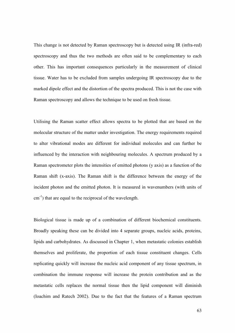
63
This change is not detected by Raman spectroscopy but is detected using IR (infra-red)
spectroscopy and thus the two methods are often said to be complementary to each
other. This has important consequences particularly in the measurement of clinical
tissue. Water has to be excluded from samples undergoing IR spectroscopy due to the
marked dipole effect and the distortion of the spectra produced. This is not the case with
Raman spectroscopy and allows the technique to be used on fresh tissue.
Utilising the Raman scatter effect allows spectra to be plotted that are based on the
molecular structure of the matter under investigation. The energy requirements required
to alter vibrational modes are different for individual molecules and can further be
influenced by the interaction with neighbouring molecules. A spectrum produced by a
Raman spectrometer plots the intensities of emitted photons (y axis) as a function of the
Raman shift (x-axis). The Raman shift is the difference between the energy of the
incident photon and the emitted photon. It is measured in wavenumbers (with units of
cm-1
) that are equal to the reciprocal of the wavelength.
Biological tissue is made up of a combination of different biochemical constituents.
Broadly speaking these can be divided into 4 separate groups, nucleic acids, proteins,
lipids and carbohydrates. As discussed in Chapter 1, when metastatic colonies establish
themselves and proliferate, the proportion of each tissue constituent changes. Cells
replicating quickly will increase the nucleic acid component of any tissue spectrum, in
combination the immune response will increase the protein contribution and as the
metastatic cells replaces the normal tissue then the lipid component will diminish
(Ioachim and Ratech 2002). Due to the fact that the features of a Raman spectrum
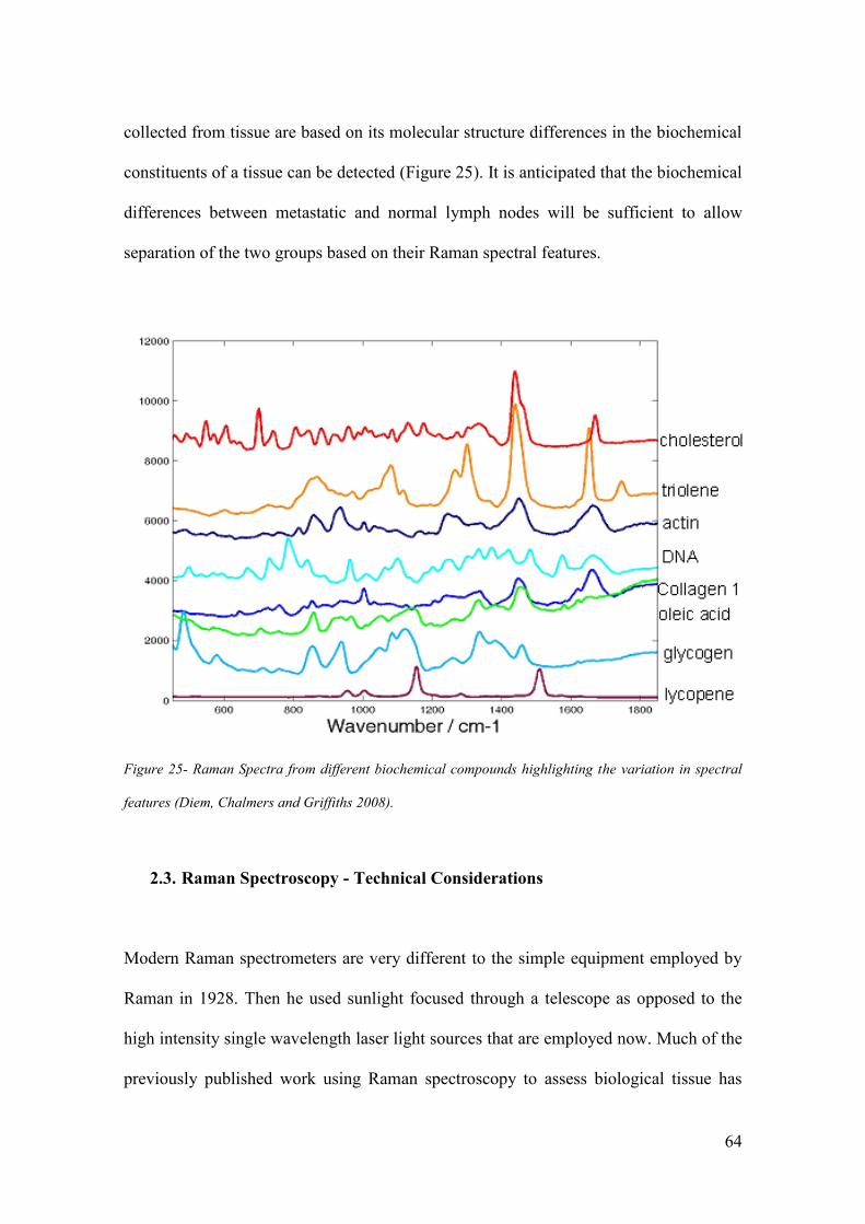
64
collected from tissue are based on its molecular structure differences in the biochemical
constituents of a tissue can be detected (Figure 25). It is anticipated that the biochemical
differences between metastatic and normal lymph nodes will be sufficient to allow
separation of the two groups based on their Raman spectral features.
Figure 25- Raman Spectra from different biochemical compounds highlighting the variation in spectral
features (Diem, Chalmers and Griffiths 2008).
2.3. Raman Spectroscopy - Technical Considerations
Modern Raman spectrometers are very different to the simple equipment employed by
Raman in 1928. Then he used sunlight focused through a telescope as opposed to the
high intensity single wavelength laser light sources that are employed now. Much of the
previously published work using Raman spectroscopy to assess biological tissue has

65
used incident light in the Near Infra Red (NIR) region. This wavelength of light is
absorbed much less readily by the tissue, causes minimal tissue damage and overcomes
the effect of fluorescence seen with visible and ultraviolet light. The wavelength of light
that is to be used in this study is 785nm.
A key consideration in Raman spectrometer design is the prevention of interference
from elastic scatter. As previously discussed the proportion of all scattered light that is
inelastic is very small. Therefore a series of filters are used to reduce this effect. In the
spectrometer used throughout this project, the B&W Tek MiniRam II (see Chapter 3), a
notch filter allows Raman peaks to be detected as close as 175cm-1
from the Rayleigh
line. Detection of the scattered light is achieved using a charged coupled device (CCD)
that allows for the measurement of a whole spectrum at once. Built into the MiniRam II
system is a thermo-electric cooler that reduces both the dark current and the background
noise. This allows the spectrometer to be used with long collection times and permits
the detection of weak optical signals.
A number of techniques have been developed to enhance the Raman signal from tissue
of interest. Although it is not intended that these techniques will be used in this project a
brief discussion is pertinent for completeness. Examples of this include resonance
Raman spectroscopy, surface enhanced Raman spectroscopy and spatially offset Raman
spectroscopy.
In resonance Raman spectroscopy the incident light is tuned so that it coincides with the
energy required for an electron to move energy level. In this way photons maybe
66
scattered up to 106 times more than using conventional Raman techniques. Thus
vibrational transitions which are too weak to be detected normally can be identified.
Surface enhanced Raman spectroscopy (SERS) is a further technique that is used to
enhance the Raman signal. In this case samples are adsorbed onto Gold or Silver
surfaces. This results in an increase in the intensity of the Raman scatter particularly
when combined with resonance Raman spectroscopy (DoItPoms 2010). The exact
mechanism for this action is still debated. It has been postulated that it may occur either
due to an increase in the electromagnetic field that then increases the interactions with
the incident light or due to the metal altering the electron energy levels of the molecule
and thus providing a resonance effect (DoItPoms 2010). The in vivo use of this
technique is currently limited by concerns about the ability of the body to excrete the
markers and thus the long term effects of retained metals. Spatially offset Raman
spectroscopy collects Raman scatter from a position several millimetres offset from the
point of excitation. This overcomes the high intensity Raman scatter from the area of
excitation which ordinarily dominates the spectra obtained. As a result this technique
has been used to probe tissue many millimetres in depth (DoItPoms 2010).
2.4. Raman Spectroscopy in a clinical setting
The use of Raman spectroscopy to identify primary tumours and differentiate them from
normal non malignant tissue has been demonstrated in a number of organs including
oesophageal (Kendall et al. 2003), laryngeal (Stone et al. 2000), bladder (Stone et al.
2004), prostate, (Stone et al. 2004) and colon (Molckovsky et al. 2003). A review of all

67
the different tissue types would be beyond the scope of this report but this section will
focus on the evidence supporting its use in breast cancer and lymph nodes.
2.4.1. Raman Spectroscopy in Breast Tissue
The first recorded spectra of human breast tissue were published in 1991 (Alfano et al.
1991). They recorded the spectra using FT-Raman spectroscopy and an excitation laser
with a wavelength of 1064 nm. Analysis was performed to compare the characteristic
spectral peaks of three normal, four benign and seven malignant specimens. They
observed differences in both the presence of particular peaks and the relative intensities.
Four key peaks were identified in normal tissue at 1078, 1300, 1445 and 1651 cm-1
. In
comparison there was an absence of these peaks at 1078 and 1300 cm-1
in the malignant
tissue. Further the intensities of peaks at 1445 and 1651 cm-1
where different in all three
tissue types. The importance of these peaks was further demonstrated in a number of
observational studies published in the 1990s and were attributed to differences in the
spectral contribution of fatty acids (FA).
Attempts to quantify what these differences equated to biochemically followed. Initial
work attributed the observed changes to contributions of fatty acids and β-Carotene
(Redd et al. 1993).
Subsequent work collected 123 spectra from 41 tissue specimens excised during breast
surgery procedures. The authors of this study used the data to compare the spectral
features of normal breast tissue with those of invasive ductal carcinoma (Frank et al.
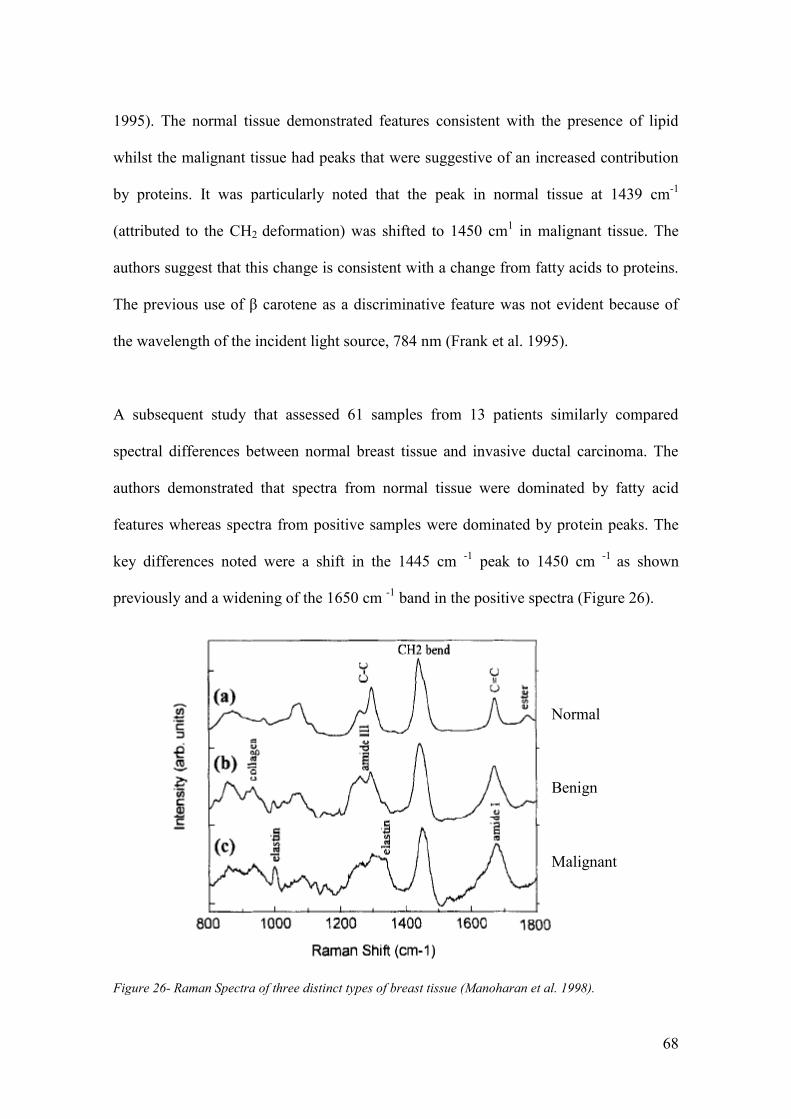
68
1995). The normal tissue demonstrated features consistent with the presence of lipid
whilst the malignant tissue had peaks that were suggestive of an increased contribution
by proteins. It was particularly noted that the peak in normal tissue at 1439 cm-1
(attributed to the CH2 deformation) was shifted to 1450 cm1 in malignant tissue. The
authors suggest that this change is consistent with a change from fatty acids to proteins.
The previous use of β carotene as a discriminative feature was not evident because of
the wavelength of the incident light source, 784 nm (Frank et al. 1995).
A subsequent study that assessed 61 samples from 13 patients similarly compared
spectral differences between normal breast tissue and invasive ductal carcinoma. The
authors demonstrated that spectra from normal tissue were dominated by fatty acid
features whereas spectra from positive samples were dominated by protein peaks. The
key differences noted were a shift in the 1445 cm -1
peak to 1450 cm -1
as shown
previously and a widening of the 1650 cm -1
band in the positive spectra (Figure 26).
Figure 26- Raman Spectra of three distinct types of breast tissue (Manoharan et al. 1998).
Normal
Benign
Malignant

69
These differences were used to differentiate between normal and malignant tissue.
Sensitivities of 100% for identifying malignant tissue, 88% for benign tissue and 94%
for normal tissue were achieved using principal component analysis (Manoharan et al.
1998). The authors of the paper accepted that the small number of samples did not allow
adequate cross validation to support these results. However the potential for the use of
Raman spectroscopy to aid clinical diagnosis of breast cancer was clearly set.
A number of groups have subsequently pursued the use of Raman spectroscopy in the
diagnosis of breast cancer. A novel approach to spectral difference analysis was adopted
by Haka et al. who in 2005 reported the creation of a breast tissue spectroscopic model.
The model was based on the analysis of 130 spectra from 58 patients undergoing breast
cancer surgery. They demonstrated that the spectra from different tissue types could be
replicated by varying the percentages of the model components, namely collagen, fat,
cholesterol, β carotene, cell cytoplasm and nucleus and calcium compounds (Figure 27).
The key spectral differences were noted to be the fat, collagen and cell cytoplasm
components. Using the component percentages they were able to distinguish between
normal and malignant tissue with 94% sensitivity and 96% specificity based on the
contributions of collagen and fat (Haka et al. 2005) (Figure 28). The authors recognised
that this was an ex vivo study based in a laser laboratory on snap frozen specimens but
they stated that it was an important step towards the clinical use of Raman spectroscopy
in breast cancer.

70
Figure 27- Normalised Raman Spectra and model fits for four distinct tissue types. The percentage of
each component included is also displayed, along with the H and E slide of the tissue type being assessed
(Haka et al. 2005.)

71
Figure 28- Scatter plot demonstrating the contribution of fat and collagen components in spectra from
different breast tissue types ( Haka et al. 2005).
The same group went on to use this analytical technique to assess the ex-vivo margin
status of tumour samples removed during breast cancer surgery. 30 samples were
assessed using Raman spectroscopy in the study from a total of 9 patients. 29 of the
samples were histopathologically reported as non malignant of which 21 were normal
tissue and 8 demonstrated benign fibrocystic change. Only 1 sample was classified as
positive , containing areas of ductal carcinoma in situ. The overall accuracy of the
algorithm was 93%, with 20/21 normal samples, 6/8 fibrocystic samples and 1/1 DCIS
samples being correctly classified. The authors recognised this as a pilot study and
accepted the limitations of such small numbers particularly in the positive group. It does

72
further demonstrate the potential diagnostic capabilities of Raman spectroscopy, based
on molecular differences, in the diagnosis of breast cancer (Haka et al. 2006).
A follow up to this study published in 2009 reported the results of real time intra
operative analysis of samples from 28 consecutive patients undergoing breast
conserving surgery. A total of 220 Raman spectra were collected from 220 samples.
Only 129 of these were deemed appropriate for analysis. The 91 that were excluded
included samples from patients who had undergone pre-operative adjuvant
chemotherapy (n=28), were having repeat surgery due to initial positive margins (n=33),
or had pathology that was positive for DCIS (n=20). 10 spectra were excluded due to
light contamination of the spectra collected. The remaining 129 spectra were classified
based on the contributions of collagen and fat to their spectra. A sensitivity of 83% (5/6)
and a specificity of 93% (114/123) was reported for the differentiation between invasive
ductal carcinoma and non malignant tissue (normal and benign pathologies)
respectively (Haka et al. 2009). However the positive predictive value of the test was
reported as only 36%. This was due to the misclassification of 4/73 and 5/9 spectra from
tissue with either fibroadenomatous or fibrocystic benign changes. As a result the
authors felt that whilst the negative predictive value of 99% was very encouraging
larger scale ex vivo and in vivo studies were required to improve their algorithm prior to
clinical implementation.
The biochemical differences between normal and malignant tissue were further
demonstrated by Chowdray et al. (Figure 29). They reported the results of 258 spectra
collected from 60 samples that were obtained from 60 patients undergoing routine
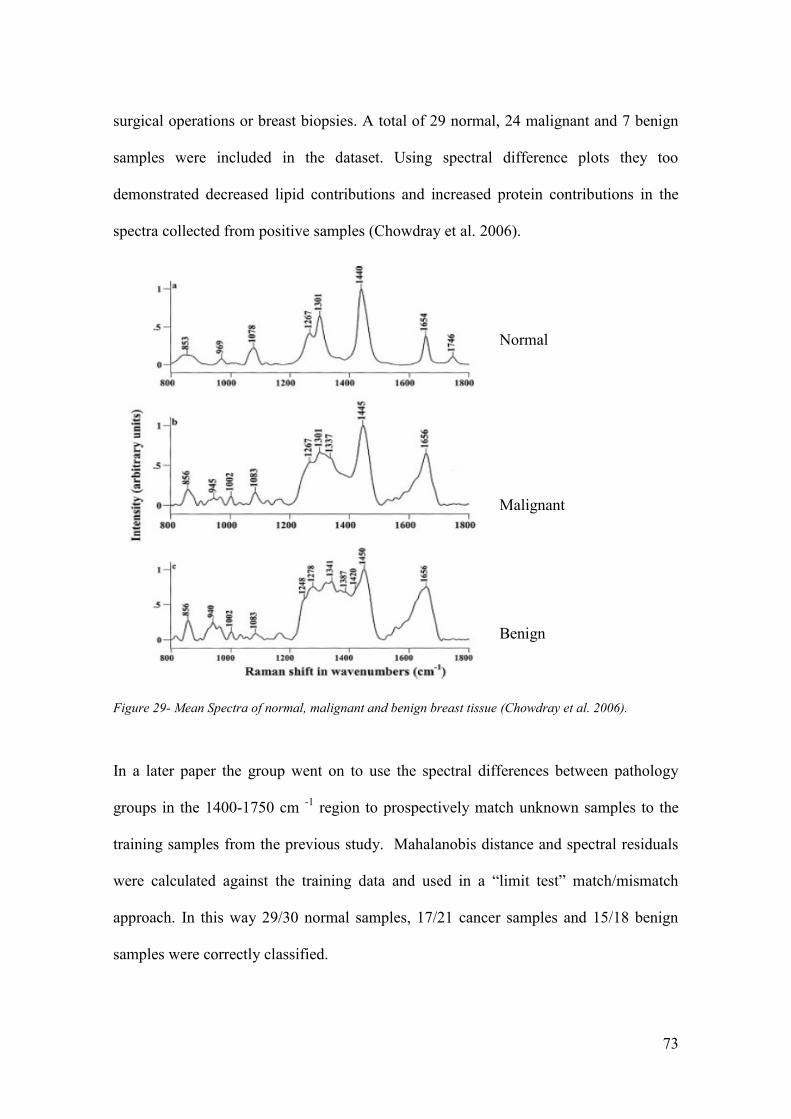
73
surgical operations or breast biopsies. A total of 29 normal, 24 malignant and 7 benign
samples were included in the dataset. Using spectral difference plots they too
demonstrated decreased lipid contributions and increased protein contributions in the
spectra collected from positive samples (Chowdray et al. 2006).
Figure 29- Mean Spectra of normal, malignant and benign breast tissue (Chowdray et al. 2006).
In a later paper the group went on to use the spectral differences between pathology
groups in the 1400-1750 cm -1
region to prospectively match unknown samples to the
training samples from the previous study. Mahalanobis distance and spectral residuals
were calculated against the training data and used in a “limit test” match/mismatch
approach. In this way 29/30 normal samples, 17/21 cancer samples and 15/18 benign
samples were correctly classified.
Normal
Malignant
Benign
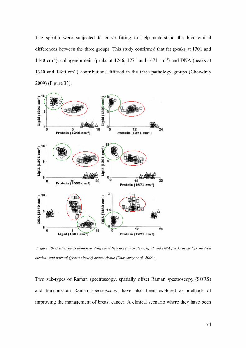
74
The spectra were subjected to curve fitting to help understand the biochemical
differences between the three groups. This study confirmed that fat (peaks at 1301 and
1440 cm-1
), collagen/protein (peaks at 1246, 1271 and 1671 cm-1
) and DNA (peaks at
1340 and 1480 cm-1
) contributions differed in the three pathology groups (Chowdray
2009) (Figure 33).
Figure 30- Scatter plots demonstrating the differences in protein, lipid and DNA peaks in malignant (red
circles) and normal (green circles) breast tissue (Chowdray et al. 2009).
Two sub-types of Raman spectroscopy, spatially offset Raman spectroscopy (SORS)
and transmission Raman spectroscopy, have also been explored as methods of
improving the management of breast cancer. A clinical scenario where they have been

75
used is the problem of positive margins after breast conserving surgery. This is a
significant cause of morbidity in breast cancer patients with up to 20% of patients
requiring further surgery to obtain adequate clearance (NHS Breast Cancer Screening
Programme 2008). One way of reducing the need for a second operation would be the
development of a technology that immediately assesses tissue margins. Research
performed on tissue models have demonstrated that using spatially offset Raman
spectroscopy (SORS) spectral features of breast cancer tumours as small as 1-2 mm in
diameter can be distinguished through up to 2 mm of normal tissue (Keller, Majumder
and Mahadevan-Jansen 2009) (Figure 31).
Figure 31- Mean Spectra of normal and breast tumour measured using SORS techniques (Keller,
Majumder and Mahadevan-Jansen 2009).
The authors state that the key spectral differences between the two tissue types are the
presence of the phenylalanine peak at 1006 cm -1
, a decreasing ratio of the 1265 to 1303
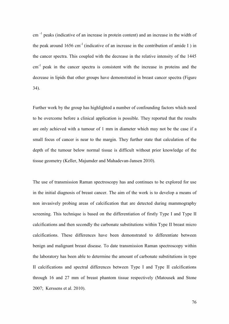
76
cm -1
peaks (indicative of an increase in protein content) and an increase in the width of
the peak around 1656 cm-1
(indicative of an increase in the contribution of amide I ) in
the cancer spectra. This coupled with the decrease in the relative intensity of the 1445
cm-1
peak in the cancer spectra is consistent with the increase in proteins and the
decrease in lipids that other groups have demonstrated in breast cancer spectra (Figure
34).
Further work by the group has highlighted a number of confounding factors which need
to be overcome before a clinical application is possible. They reported that the results
are only achieved with a tumour of 1 mm in diameter which may not be the case if a
small focus of cancer is near to the margin. They further state that calculation of the
depth of the tumour below normal tissue is difficult without prior knowledge of the
tissue geometry (Keller, Majumder and Mahadevan-Jansen 2010).
The use of transmission Raman spectroscopy has and continues to be explored for use
in the initial diagnosis of breast cancer. The aim of the work is to develop a means of
non invasively probing areas of calcification that are detected during mammography
screening. This technique is based on the differentiation of firstly Type I and Type II
calcifications and then secondly the carbonate substitutions within Type II breast micro
calcifications. These differences have been demonstrated to differentiate between
benign and malignant breast disease. To date transmission Raman spectroscopy within
the laboratory has been able to determine the amount of carbonate substitutions in type
II calcifications and spectral differences between Type I and Type II calcifications
through 16 and 27 mm of breast phantom tissue respectively (Matousek and Stone
2007; Kerssens et al. 2010).

77
These papers suggest that, by exploiting the differences in protein and lipid
contributions to spectra collected from normal and malignant breast tissue, Raman
spectroscopy could be used in a number of clinical situations pertaining to breast cancer.
As has been demonstrated this may include the assessment of margin status after breast
conserving surgery or potentially the assessment of core biopsy samples that are used in
the initial diagnosis of the disease. Differences in the calcification types can also be
detected using Raman spectroscopy and these could reduce the morbidity associated
with breast screening.
The ability of Raman spectroscopy to differentiate between normal and malignant tissue
is important in this study. Although the tumour itself will not be assessed, metastatic
cells that spread from the breast to the lymph nodes have very similar histological
properties to the original tumour. It is anticipated that the differences previously
described between normal and metastatic tissue will have different spectroscopic
features and that these differences can be exploited to differentiate between normal and
metastatic nodes.
2.4.2. Raman Spectroscopy in Lymph Nodes
To date there have been very few papers published that document the use of Raman
spectroscopy for the assessment of lymph nodes. One of the first papers that reported
Raman spectral assessment of axillary lymph nodes used the technique as a method of
examining whether silicon breast implants had split. Axillary node tissue specimens
were obtained during surgery following silicone implant leak and compared to nodes
78
from patients with lung cancer that were undergoing lymph node dissection. The
authors of the paper did not report in great detail the peak assignments of the spectra
that they acquired other than to comment that peaks above 1000 cm-1
were due to lipid
components. The presence of silicon was clearly demonstrated and the authors
concluded that Raman spectroscopy could provide a rapid diagnostic test that could be
used in this context (Frank et al. 1993) (Figure 32).
Figure 32- Spectra of normal lymph nodes and those upstream of a silicone implant leak. The added
peaks (circled in blue) between 400 and 750 cm-1
allow for the differences to be distinguished (adapted
from Frank et al. 1993).

79
A further study published in 2005 used Raman spectroscopy to confirm the presence of
silicone within the axillary lymph nodes of 71/96 patients with breast implants. The
authors did not comment on the features of the lymph node spectra other than to
highlight the presence of polymethysiloxane and polyurethane peaks in the spectra
obtained from patients with implants. The sensitivity of Raman spectroscopy at
detecting changes in the lymph node associated with silicone implants was worse than
standard pathological assessment but was felt to relate to the small area of the node that
was assessed using Raman spectroscopy (Katzin et al. 2005).
To date only one group (ours) has used Raman spectroscopy to assess the presence or
absence of metastatic cells within human lymph nodes in breast cancer. 59 lymph node
samples were collected from 58 patients undergoing axillary lymph node excision due
to breast cancer. Raman spectroscopy mapped images were created from 7 μm sections
of tissue with a step size of 100 μm in the x and y direction. The differences in the mean
spectra of positive versus negative nodes suggested that there were decreases in the
DNA and tyrosine contributions within the negative nodes. It was interesting to note
that the lipid contribution appeared to be similar in both groups, in contrast to the
findings in the breast papers previously reviewed. Principal component fed linear
discriminant analysis (PCA fed LDA) was used to create a pathology classification
model. This achieved a sensitivity of 91% and a specificity of 93% at differentiating
between the positive and negative nodes. Whilst these results were very encouraging the
authors recognised that the time taken to produce these mapped images, 12 to 120
hours, was inadequate for intra operative use (Smith 2005).

80
A potential method of overcoming the disadvantage of mapped images was to use a
probe and collect spectra from a greatly reduced but evenly spread area of tissue. The
effects of this change were modelled by selecting 5 and 10 points at equally spaced
positions across the mapped images of 53 and 47 nodes respectively . The estimated
time to collect the spectra obtained from these points was 9 and 18 minutes in the two
groups. Sensitivities of 71%, in the 5 probe point group, and 81% , in the 10 probe point
group, with specificities of 97% in both groups were achieved based on a cross
validated model (Horsnell et al. 2011). These results support the use of a Raman
spectroscopy probe for the assessment of axillary lymph nodes as they produced results
that were equivalent to both frozen section and touch imprint cytology, in a time frame
that would be suitable for intra-operative use. The low sensitivity was attributed to the
small total area of the node assessed, 2800μm3 and 5600 μm
3 in the two respective
groups. The authors felt that the increase in sensitivity that was achieved by doubling
the total area assessed in the 5 and 10 point group could be further enhanced by using
probes that collected spectral data from an even greater tissue area (Horsnell et al.
2011).
Lymph nodes from patients with oesophageal cancer have also been investigated using
Raman spectroscopy. 76 halved lymph node samples from 57 patients were collected
and snap frozen at the time of surgery. 30 of these samples were said to be positive for
cancer and 46 were negative for cancer after histopathological analysis. The samples
were then assessed using both Raman and FTIR spectroscopy within a laser laboratory.
The mean Raman spectra of positive and negative nodes were compared and
demonstrated lipid, carbohydrate and protein peaks in the negative nodes and stronger

81
nucleic acid peaks in the positive nodes. PCA fed LDA was then used to assess the
diagnostic capability of these differences. Cross validated results achieved a sensitivity
of 97% and a specificity of 89% for the differentiation of negative and positive nodes.
The authors of this study concluded that these results provided a “launchpad” for the
development of in vivo applications of Raman spectroscopy in lymph node diagnostics
(Isabelle et al. 2008).
The use of Raman spectroscopy as a diagnostic tool for the assessment of axillary
lymph nodes remains in its infancy. Whilst the studies to date have been encouraging
they have been limited by low sample numbers and have been laboratory based using
frozen tissue. This study will be the first to move the spectrometer out of the laboratory
into the operating theatre and will assess freshly excised human tissue.
2.4.3. Alternative optical methods of assesing lymph nodes
Other forms of optical spectroscopy have been used to assess lymph nodes. These
include elastic scattering and infrared spectroscopy. Elastic scattering spectroscopy
(ESS) is a technique that is based on the elastic scattering of light. Short pulses of white
light from a source such as a Xenon lamp are delivered to the tissue. Scattered light
which has the same wavelength as the incident light is collected by a collection fibre
that is offset from the light source. Spectra collected in this way are sensitive to the
sizes, refraction indices and structures contained within sub cellular tissue components.
A recent study used this technique to create a diagnostic algorithm based on the results
of 331 negative and 30 positive lymph nodes. They went on to test an independent data

82
set of 129 samples at the time of surgery and achieved a sensitivity of 76% (69% with
micrometastases) and a specificity of 96% at differentiating between positive and
negative nodes (Keshtgar et al. 2010) (Figure 33 and 34).
Figure 38- False colour coded scan of a node, using optical spectroscopy, showing a single metastasis
alongside its histology (H and E) image ( Keshtgar et al. 2010).
Figure 34- Mean elastic scattering Spectra from 331 normal nodes and 30 metastatic nodes with
standard deviations (Keshtgar et al. 2010).
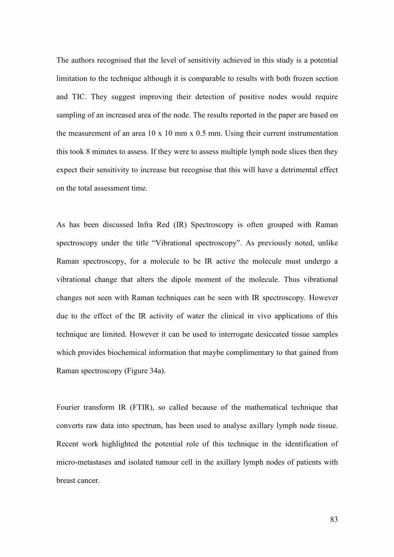
83
The authors recognised that the level of sensitivity achieved in this study is a potential
limitation to the technique although it is comparable to results with both frozen section
and TIC. They suggest improving their detection of positive nodes would require
sampling of an increased area of the node. The results reported in the paper are based on
the measurement of an area 10 x 10 mm x 0.5 mm. Using their current instrumentation
this took 8 minutes to assess. If they were to assess multiple lymph node slices then they
expect their sensitivity to increase but recognise that this will have a detrimental effect
on the total assessment time.
As has been discussed Infra Red (IR) Spectroscopy is often grouped with Raman
spectroscopy under the title “Vibrational spectroscopy”. As previously noted, unlike
Raman spectroscopy, for a molecule to be IR active the molecule must undergo a
vibrational change that alters the dipole moment of the molecule. Thus vibrational
changes not seen with Raman techniques can be seen with IR spectroscopy. However
due to the effect of the IR activity of water the clinical in vivo applications of this
technique are limited. However it can be used to interrogate desiccated tissue samples
which provides biochemical information that maybe complimentary to that gained from
Raman spectroscopy (Figure 34a).
Fourier transform IR (FTIR), so called because of the mathematical technique that
converts raw data into spectrum, has been used to analyse axillary lymph node tissue.
Recent work highlighted the potential role of this technique in the identification of
micro-metastases and isolated tumour cell in the axillary lymph nodes of patients with
breast cancer.

84
Figure 34a- Spectra obtained from the same sections of human cervical tissue using Raman (blue) and IR
(green) spectroscopy. This highlights the very different spectral information available from the two
techniques and why they can be used as complimentary tools to each other (Adapted from images held
within our own department).
In this study 20 nodal tissue sections from 20 patients were cut from formalin fixed
paraffin embedded archived tissue blocks. Spectra were collected in 6.25 μm steps such
that a 1 mm x 1 mm tissue black was represented by 160 x 160 spectra. Higher cluster
analysis was used to reproduce histological features of the cut lymph node surface
(Figure 35) (Bird et al. 2009).

85
Figure 35 - FTIR Mapped images (centre and right) that show excellent correlation with the associated
histology slide (left) (Bird et al. 2009).
Good correlation was achieved in comparison to H and E slides of the same area. Using
this technique macrometastases, micrometastases and isolated tumour cells were
identified although no attempt was made at creating a classification model based on the
results.
The use of FTIR in the assessment of lymph nodes from other areas of the body has also
been published. When used to differentiate between positive and negative lymph nodes
from patients with oesophageal cancer sensitivities of 91% and specificities of 85%
were achieved. Spectra from positive nodes displayed a greater contribution of protein
and DNA than those spectra collected from negative nodes (Isabelle et al. 2008). FTIR
was also used in a study that assessed the touch imprint samples collected during
parathyroid surgery. The ability to correctly identify the parathyroid, thyroid or lymph
nodes during a parathyoidectomy is vital and can often only be confirmed by the
pathological assessment. Clear spectral differences were evident between these tissue
types. In particular it was noted that the lymph nodes displayed strong lipid peaks at
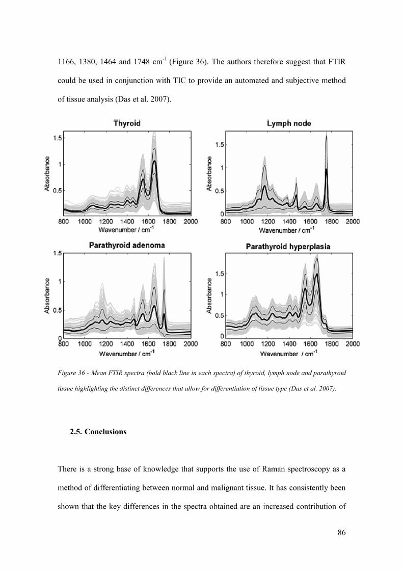
86
1166, 1380, 1464 and 1748 cm-1
(Figure 36). The authors therefore suggest that FTIR
could be used in conjunction with TIC to provide an automated and subjective method
of tissue analysis (Das et al. 2007).
Figure 36 - Mean FTIR spectra (bold black line in each spectra) of thyroid, lymph node and parathyroid
tissue highlighting the distinct differences that allow for differentiation of tissue type (Das et al. 2007).
2.5. Conclusions
There is a strong base of knowledge that supports the use of Raman spectroscopy as a
method of differentiating between normal and malignant tissue. It has consistently been
shown that the key differences in the spectra obtained are an increased contribution of

87
lipid in the normal tissue relative to malignant tissue and an increased contribution of
protein and DNA in the malignant tissue relative to the normal tissue. These results are
supported by FTIR results in axillary, oesophageal and head and neck cancers.
A number of groups are now trying to harness these techniques as a means of improving
the management of breast cancer. This project will aim to build on these previous
studies to demonstrate that Raman spectroscopy could be used within the theatre setting
to assess axillary lymph nodes. If this is proven to be the case then Raman spectroscopy
has the potential to be the first method that can fulfil all the features that were
previously highlighted as the requirements of an ideal method of intra-operative
analysis.

88
3. Towards using a probe in theatre.
3.1. Introduction
As discussed in the previous chapter earlier in vitro work has demonstrated the potential
for the use of Raman spectroscopy to differentiate between malignant and non
malignant lymph nodes in breast cancer (Smith 2005; Horsnell et al. 2011). However
this work had a number of significant draw backs that would need to be overcome if
Raman Spectroscopy were to be used in the clinical setting.
1. The time taken for spectral acquisition – The mapping images previously used to
differentiate between the two pathologies were obtained over time frames that
would have precluded their use in an intra operative setting.
2. The equipment used – Previous studies have utilised expensive laboratory based
systems that would be beyond the reach of most surgical units. The footprint of
the instruments would also have significant implications as safe and suitable
storage facilities would be difficult.
3. The environment – The previous work had been performed within a specialised
spectroscopy laboratory in standardised conditions. If, as is envisaged, the node
assessment were to take place within the operating theatre these conditions could
not be easily replicated.

89
4. Exposure to node markers – The lymph nodes in previous studies were obtained
following either axillary sampling procedures or during axillary dissections. At
the time of that study SLNB was not routinely performed. As a result there was
no dye used to identify the lymph nodes. There is significant concern with
regard to the affect this will have on the diagnostic capability of the technique
because dyes used to orientate the specimens within the lab demonstrated
significant fluorescence.
5. Sample preparation - Previous work has demonstrated the efficacy of Raman
spectroscopy using sections of lymph node material. This would significantly
add to the overall assessment time as well as render assessment within the
operating theatre impossible without significant further investment in equipment
and expertise.
In this chapter experimental work will be presented that has been designed to determine
if and how these problems could be overcome. A key part in this has been the selection
of the spectrometer. Therefore the probe based Raman spectrometer that was selected
for use in this project will be described and its capabilities in this setting reviewed.
Results of a small feasibility study that was performed using human axillary lymph
nodes will be reported before concluding the chapter with some experiments that looked
at the effect of the theatre environment on spectral acquisition.

90
3.2. The Raman Spectrometer
The first and most significant hurdle that had to be overcome in this project was the
selection of equipment that could be used outside of the laboratory. As previously
discussed mathematical modelling had suggested that a probe based system could be
used to assess axillary lymph nodes rather than the more traditional mapping techniques
that had been used in the past (Horsnell et al. 2011).
The B&W Tek MiniRam II (B&W Tek, Newark, DE, USA) Raman spectrometer was
purchased for use in this project and is utilised in all of the experimental data reported
in this thesis. This spectrometer features a 785nm laser with a spot size diameter of
85μm and a maximum power of 300mW at the probe tip. The laser light is delivered via
a hand held probe and a distance regulator, that fits the tip of this probe, ensures that
samples are positioned 59mm from the tip of the probe. This distance has been
determined by the manufacturer as the optimum position for spectral acquisition.
Collected light is passed through a spectrometer that provided spatial resolution of
10cm-1
with a built in thermo-electrically cooled CCD (Figure 37). The nominal ocular
hazard distance was calculated at less than 10cm and was a key feature of the local rules
that were designed for its use.
The whole system is both lightweight and has a small footprint that would be ideal for
use within the operating theatre setting (Figure 38). Further the price of the
spectrometer, circa £12000, is significantly less than most laboratory based systems and
the equipment used for intra-operative assessment based on molecular assays.

91
Figure 37 – A stylised diagram of the Raman spectrometer device.
Figure 38- The B&W Tek © Mini Ram II on a standard theatre trolley, with a standard 30 cm ruler in the
foreground illustrating the small footprint of the product.

92
To overcome any daily variation in spectral acquisition standard measurements were
collected at each session. Spectra from green glass, pipette tip, and cyclo-hexane were
recorded and stored and then used later to calibrate the spectral data. A dark scan was
recorded at the start of each session and is subtracted from the spectra recorded in the
subsequent session. This overcomes the “hot” pixels on the CCD and is as per the
manufacturers recommendations.
3.3. Experiment 1 - Depth of Spectral Acquisition.
Prior to embarking on clinical studies to ascertain the efficacy of the system if was felt
that a greater understanding of the capabilities of the probe based system was required.
As has been discussed previous work assessing axillary lymph nodes has been
performed using Raman spectroscopy systems that collected spectral information from
an area of 45 μm2 and from samples that were only 7 μm thick. This would not be
amenable to intraoperative use as the time taken to collect mapped images was between
12 and 120 hours. Further the time taken for tissue preparation would not be acceptable
in an intra-operative setting and is one of the disadvantages of frozen section analysis
that is used currently.
When designing an ideal diagnostic tool it was felt that minimal tissue preparation
would be desirable as this would reduce the time taken to output a result and reduce the
need for added expertise and equipment. Thus the design of the clinical part of this
study anticipated that the node would simply be denuded of surrounding axillary fat and
then bisected. Spectra would then be acquired from the two halves of the node

93
individually. An appreciation of the depth from which the probe collected scattered light
was vital both in samples with macrometastases and micrometastases (Figure 39).
Figure 39- An illustration of the importance of sampling depth using a Raman probe to try and gain an
appreciation of what might be “seen” using the system.
3.3.1. Experiment 1 – Methods.
To determine the depth from which the probe receives scattered light an experimental
model was created. This was designed such that a standard material could be advanced
towards the probe through a variety of different media. As demonstrated in figure 44 a
standard 20ml syringe (BD, Oxford, UK) was used to contain the media being tested.
Four experimental media, standard room air (i.e. an empty space), sterile water for
injection (Baxter, Newbury, UK), standard olive oil (Napolina, Liverpool, UK) and lard
(everyday value range, Tesco, UK) were used. 15 ml of each media (aside from the
room air) was placed within the syringe whilst in a liquid state. Olive oil and lard were

94
chosen as they most closely resembled the fat composition of a lymph node. This
composition has previously been estimated as containing 29% saturated fats, 57%
unsaturated fats, and 9% polyunsaturated fats (Pond and Mattacks, 2003; US and
Finnish Food Database 2009).
A 1 mm3 block of PTFE was then placed on the surface of the media. This was attached
to a translation stage (Thorlabs, Ely, UK) that allowed the block to be advanced in
0.5mm steps through the media under investigation (Figure 40).
Figure 40- The experimental set up to measure the depth from which spectral information is gathered
In the first part of the experiment the PTFE block was placed at the maximal distance
away from the probe tip (14.5mm) and then advanced in 0.5mm intervals. 5 spectra
were obtained at each of these positions and the process was repeated for all 4 media.

95
The MiniRam II was used throughout and each spectra was obtained by combining 16 x
1 sec acquisitions. Control spectra from each of the media and the PTFE were also
recorded. In the second part of the experiment an attempt was made to approximate the
volume from which spectral information was collected. The experimental set was
modified so that the PTFE standard could be moved in both the z (up and down) and y
(side to side) plane. The chamber was filled with olive oil, which not only closely
resembled the fatty composition of a lymph node but which also, due to its liquid state
at room temperature was easiest to handle. 5 spectra were collected from 25 different
positions. The PTFE block was moved in 1.0 mm steps to 4 mm from the optimum
point in the z direction and 0.25 mm steps to 1mm offset in the y direction. The initial
measurement was made with the PTFE block at 0mm offset in both the z and y plane. It
was then moved in the y plane before being returned to the initial position and then
moved in the z direction. Further spectra were obtained at each y position before
returning to the y=0 position and altering the z position again. Spectra were obtained as
described for the first part of the experiment and all data was then transferred to a
desktop PC for interpretation using Matlab ® software.
3.3.2. Experiment 1 - Results.
Examination of the spectra from the PTFE block revealed a peak at 738cm-1
that was
not present in any of the other control media. The intensity of this peak was calculated
when the PTFE block was at the optimal distance from the probe tip (5.9 mm) in all the
media. This figure was then used to calculate the relative intensity of the 738 cm-1
peak
at increasing distances from the optimal point by calculating an intensity percentage at

96
each 0.5mm step in the first experiment and each position in the second experiment.
These percentages were plotted to produce curves for the change in intensity with
increasing offset for each of the four media (Figure 41, 42). In the curves the gradient of
the slope has started to level out by 3mm from the optimal point of the probe although
the clearest peaks are recorded at less than 1.5mm. The distinct differences seen using
lard may have been explained by the solid nature of lard at room temperature. Thus
maintaining a consistent volume of the media between the probe tip and the PTFE was
difficult. The results of the second part of the experiment were plotted graphically to
give a visual idea of the volume of tissue from which spectral information is collected
using this system (Figure 44). It was evident that beyond 0.5 mm movement in the y
direction there was no discernable contribution of the PTFE block.
3.3.3. Experiment 1 – Conclusions.
Although these results were part of an observational study they do allow some
appreciation of the volume from which spectral information could be gathered using
this MiniRam II system. Before proceeding to discuss the results further it is important
to state that definitive interpretation of the results does need to be carried out cautiously
as it is likely that the optical properties of a lymph node and media used in this
experiment will differ. In particular the elastic scatter of tissue will cause many more
transverse scattering events than these media and thus the results were used as a guide
when discussing the technique with clinicians rather than an absolute.

97
Within this media it is clear that beyond 3 mm depth the contribution of the PTFE
block is negligible and that beyond 0.5 mm lateral movement the contribution is non
discernable. This is the point beyond which any surface of the block is in line with the
laser. In this media as long as a part of the block is in line with the laser then spectral
information will be acquired to a depth of 3 mm. Transposing this to tissue the best
possible volume from which spectral information from a metastatic deposit could be
detected is given by the formula
(π x (diameter of the deposit 2 )) x (height of the deposit +3 mm)
If we relate this to a macrometastases, which by definition is at least 2 mm in diameter
the maximum size of a node sample that a 2 mm deposit could be detected in is a node
visualised as a cylinder of 4 mm diameter x 5 mm depth. The volume of tissue in which
it will be detected is 62.8 mm3 (Figure 43, 44).
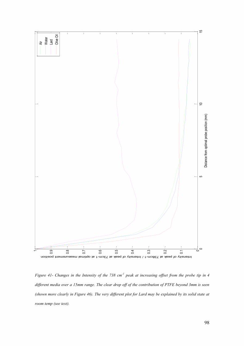
98
05
1015
0
0.1
0.2
0.3
0.4
0.5
0.6
0.7
0.8
0.91
Dis
tanc
e fro
m o
ptim
al p
robe
pos
ition
(m
m)
Intensity of peak at 738cm-1 / Intensity of peak at 73cm-1 at optimal measurement position
Air
Wat
er
Lard
Oliv
e O
il
Figure 41- Changes in the Intensity of the 738 cm-1
peak at increasing offset from the probe tip in 4
different media over a 15mm range. The clear drop off of the contribution of PTFE beyond 3mm is seen
(shown more clearly in Figure 46). The very different plot for Lard may be explained by its solid state at
room temp (see text).

99
Figure 42- Changes in the Intensity of the 738 cm-1
peak at increasing offset from the probe tip in 4
different media as shown in Figure 41. In this figure this is shown over a 5mm range to give greater
clarity.

100
Figure 43- An illustration of the total volume of tissue within which macro-metastases of at least 2mm in
diameter could be detected (not to scale).
Lymph node metastases are first found within the medulla of the nodes. It was thus
decided that all nodes will be bisected and samples taken from the inner cut surface.
Thus the MiniRam II should, if this model is projected forward, be able to detect all
macrometastases in lymph nodes that are smaller or equal to 10 mm x 4 mm. This
information was used to determine the clinical study design. It has previously been
reported in a review of 1249 axillary nodes that 47% were less than 5 mm in diameter ,
34% were between 5 and 9 mm in diameter , 17% were between 10 and 20 mm and 2%
were greater than 20 mm in diameter (Obweseger et al.2000). Therefore there was
obvious concern that as a result macrometastases may be missed in 19% of nodes. It is
reasonable to suggest that this situation would be mitigated because the first colonies of
metastatic cells will establish themselves within the medulla of the lymph node and that
spectra would be collected from the inner cut surface of the node. Further methods of
increasing the volume of node assessed would be to divide the node into further
sections. The tissue used in the real time clinical part of this study will be relied upon to

101
guide patient treatment. Further manipulation of the tissue was thus deemed
inappropriate. As will be discussed in Chapter 4, an alternative method of increasing
the volume tested would be to collect spectra from both the inner and outer surface of
the node. In this way it could be anticipated that the depth of collection may be doubled.
Accepting the assumptions commented on above, for micrometastases, of at least 0.2
mm in diameter the total depth of collection from a lymph node sample would be 3.2
mm and the volume from which micrometastases could be detected would be only 0.8
mm3.
Figure 44- 3D plot demonstrating the intensity profile of the B and W Tek Miniram II as determined in
the depth experiment.

102
3.4. Experiment 2 - Feasibility Study.
Prior to launching into a theatre based study it was felt prudent that a feasibility study
should be performed with the equipment that was planned to be used in the theatre
setting. This not only allowed confirmation that the modelling studies were reproducible
using an actual Raman spectroscopy probe but it also afforded the opportunity to
overcome any technical issues prior to carrying out spectral acquisition within the
operating theatre environment.
3.4.1. Experiment 2 – Methods.
Following local ethical approval (approval code 01/158G – “The Development of
Raman Spectroscopy in the Diagnosis of Breast Cancer”) lymph nodes were collected
from a small cohort of 20 consecutive patients presenting with newly diagnosed
invasive breast cancer. All patients were consented prior to taking part. They all
underwent either a sentinel lymph node biopsy or an axillary node dissection as part of
an operation that also included a wide local excision or a mastectomy to excise the
primary breast tumour. These procedures were performed at Russell Hall Hospital,
Dudley by a single consultant surgeon. Pre-operative preparation for the SLNB
followed national standards. Not more than 24 hours prior to surgery patients received a
peri-tumoral injection of radio-labelled Technetium 99m
and immediately prior to
surgery the surgeon injected patent V blue dye into the subcutaneous tissue overlying
the tumour.

103
During the operative procedure the node was identified and its status as the sentinel
node confirmed by measuring the radioactivity of the node, using a hand held gamma
probe. The visual “blueness” of the node was also recorded on an analogue scale of 0-3
(0= not blue, 1= faint blue, 2 = mild blue, 3= strong blue). The node was then excised
and denuded of fatty tissue before being divided into two halves. One part was sent for
routine histopathological examination and the other half was used for research purposes.
The sample for research use was placed in a cyrovial, labelled and immediately
immersed in liquid nitrogen. The sample was then transported to the histopathology
laboratory at Russell’s Hall Hospital, Dudley. Here it was stored at approximately -48ºC
prior to being transferred to the research department at Gloucestershire Hospitals NHS
Trust. Once in Gloucester the nodes were stored within the pathology laboratory freezer
at a temperature of -80ºC. Sections of each node were cut, according to local protocols,
by staff within the pathology department for preparation of a standard H&E slide. These
slides were examined by a consultant histopathologist to define the “gold standard”
result for each of the nodes.
The remaining tissue was transferred to the research laboratory where it remained
frozen at temperatures of approximately -80ºC. This tissue was used for experiments
using the portable Raman system. All samples used in these experiments were defrosted
for 30 minutes at laboratory temperature (21ºC) prior to spectroscopic analysis within a
laser laboratory. Following this spectra were collected as described in Chapter 4.2 for
freshly excised nodes. Data was then transferred to a desktop PC and all spectra were
pre-processed by a standard set of processes which will be discussed in more detail at

104
the start of Chapter 4. Matlab® software was then used to interpret the spectra. Mean
spectra were calculated for each pathological group. Peak assignment was performed
based on tables held within the department. The statistical significance of differences
between the intensities of these peaks in each group was calculated using the Student’s
t-test. Principal component analysis (PCA) and linear discriminant analysis (LDA)
(details described further in Chapter 4) was then used to split the two groups and mimic
a diagnostic process.
3.4.2 Experiment 2 – Results.
A total of 38 nodes were analysed in this study from 17 different patients (mean 2.35
nodes, range 1-4). 25 of the nodes studied were reported by histopathology as negative
(i.e. no metastases) and 13 were reported as positive (i.e. metastases present). All of the
positive nodes were be defined as macrometastases. A total of 3602 spectra were
obtained from the 38 lymph nodes assessed. A mean of 95 spectra were obtained from
each node (range 25 -100 spectra) (Table 6).
Nodal Status based on
H and E assessment
Total Number of Nodes Total Spectra Numbers Mean number of
Spectra per node
Negative 25 2384 95.4
(Range 95 -100)
Positive 13 1218 93.7
(Range 25 -100)
Table 6- Details of data included in the feasibility study split into two groups based on H and E
assessment.

105

106
Figure 45- Mean spectra for nodes defined as normal (i.e. negative) (n=25, spectra=2384) and positive
(i.e. contains metastases) (n=13, spectra=1218) by H and E assessment in the feasibility experiment. 10
peaks identified using tables held within the department marked.
The first stage in the analysis of this dataset was to calculate mean spectra for each of
the two histological groups (Figure 45). 10 peaks across the spectra were identified and
the intensities of these peaks were analysed to determine differences between the two
histological groups (Figure 45). The statistical differences between the intensities of the
ten peaks in the two histological groups were calculated using the Student’s t-test (Table
7).
Peak
Number
Peak
Position
(cm-1
)
Mean Intensity of the peak
in H and E defined negative
samples
(spectra no. = 2384)
(SD and SEM)
Positive Intensity of the peak
in H and E defined positive
samples
(spectra no. = 1218)
(SD and SEM)
P Value
(Student’s
t-test)
1 874 0.0367
(0.003,0.00006)
0.0366
(0.002, 0.00006)
0.2593
2 1087 0.0421
(0.0063, 0.00013)
0.0426
(0.005, 0.00015)
0.0209
3 1159 0.0222
(0.0028,0.00006)
0.0232
(0.0026, 0.00007)
0.0001
4 1272 0.037
(0.0053, 0.0001)
0.0379
(0.004, 0.0001)
0.0001
5 1305 0.051
(0.01, 0.00024)
0.0522
(0.01, 0.0003)
0.0033
6 1444 0.0663
(0.02, 0.0004)
0.0677
(0.017, 0.0005)
0.0039
7 1458 0.0521 0.0546 0.0001

107
(0.0132, 0.0003) (0.01, 0.0003)
8 1530 0.0142
(0.0032, 0.00007)
0.0152
(0.0028, 0.00008)
0.0001
9 1660 0.0327
(0.0067, 0.00014)
0.0331
(0.0051, 0.00015)
0.0754
10 1751 0.0142
(0.0011, 0.000023)
0.0142
(0.001,0.00003)
1.0
Table 7- The mean intensities of the 10 peaks labelled in figure 45 for H and E defined negative and
positive nodes.. The p-values given by a Student’s t-test represent the statistical significance of the
difference between the means of the intensities of each peak in the two histological groups (SD= standard
deviation , SEM= standard error of the mean)
Statistically significant differences were calculated for the intensities of 7 of the ten
peaks. These peaks were at 1087, 1159, 1272, 1305, 1444, 1458 and 1530cm-1
. These
peaks may represent a variety of biochemical constituents including lipid, protein and
nucleic acids. The implications of these differences will be discussed in greater detail
when the results of the larger intraoperative study are discussed.
In the second stage of spectral interpretation principal component analysis (PCA) was
used to help separate the two histological groups. As is explained in Chapter 4.4.1.2
PCA allows simplification of the data into fewer variables (loads) whilst retaining the
overall information. Self programmed Matlab® functions were used to determine the
loads and the contribution that they made to each spectra (scores). Differences in the
scores for the first 10 principal components of each histological group where analysed

108
using a Student’s t-test and differences between the first 9 were shown to be statistically
significant (Table 8).
Principal
Component
(PC)
Mean Value for the score of each PC
in H and E defined negative nodes
(spectra no.= 2384)
(SD and SEM)
Mean Value for the score of each
PC in H and E defined negative
nodes (spectra no.= 1218)
(SD and SEM)
p value
1 -0.0053
(0.1588, 0.0032)
0.0117
(0.1348, 0.004) 0.0019
2 -0.0056
(0.121, 0.002)
0.0125
(0.0113, 0.00034) 0.0001
3 -0.0015
(0.014, 0.000281)
0.0034
(0.009, 0.0003) 0.0001
4 -0.0018
(0.0125, 0.0003)
0.0041
(0.0067, 0.0002) 0.0001
5 -0.0009
(0.0122, 0.0002)
0.002
(0.0063, 0.0002) 0.0001
6 0.0007
(0.0097,0.0002)
-0.0016
(0.007, 0.0002) 0.0001
7 -0.0009
(0.01, 0.0002)
0.002
(0.0046, 0.0001) 0.0001
8 -0.0017
(0.0069, 0.0001)
0.0038
(0.0076, 0.0002) 0.0001
9 -0.0011
(0.0067, 0.0001)
0.0024
(0.0073, 0.0002) 0.0001
10 0
(0.0033, 0.0001)
-0.0001
(0.01, 0.0003) 0.6649
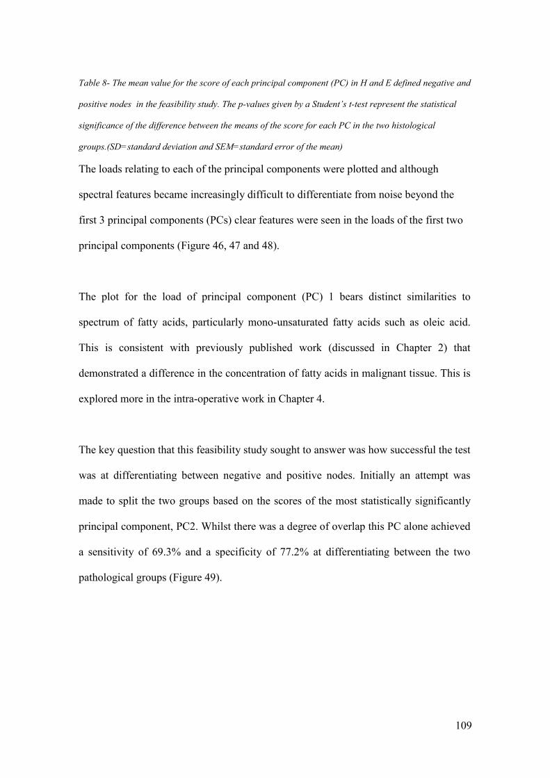
109
Table 8- The mean value for the score of each principal component (PC) in H and E defined negative and
positive nodes in the feasibility study. The p-values given by a Student’s t-test represent the statistical
significance of the difference between the means of the score for each PC in the two histological
groups.(SD=standard deviation and SEM=standard error of the mean)
The loads relating to each of the principal components were plotted and although
spectral features became increasingly difficult to differentiate from noise beyond the
first 3 principal components (PCs) clear features were seen in the loads of the first two
principal components (Figure 46, 47 and 48).
The plot for the load of principal component (PC) 1 bears distinct similarities to
spectrum of fatty acids, particularly mono-unsaturated fatty acids such as oleic acid.
This is consistent with previously published work (discussed in Chapter 2) that
demonstrated a difference in the concentration of fatty acids in malignant tissue. This is
explored more in the intra-operative work in Chapter 4.
The key question that this feasibility study sought to answer was how successful the test
was at differentiating between negative and positive nodes. Initially an attempt was
made to split the two groups based on the scores of the most statistically significantly
principal component, PC2. Whilst there was a degree of overlap this PC alone achieved
a sensitivity of 69.3% and a specificity of 77.2% at differentiating between the two
pathological groups (Figure 49).
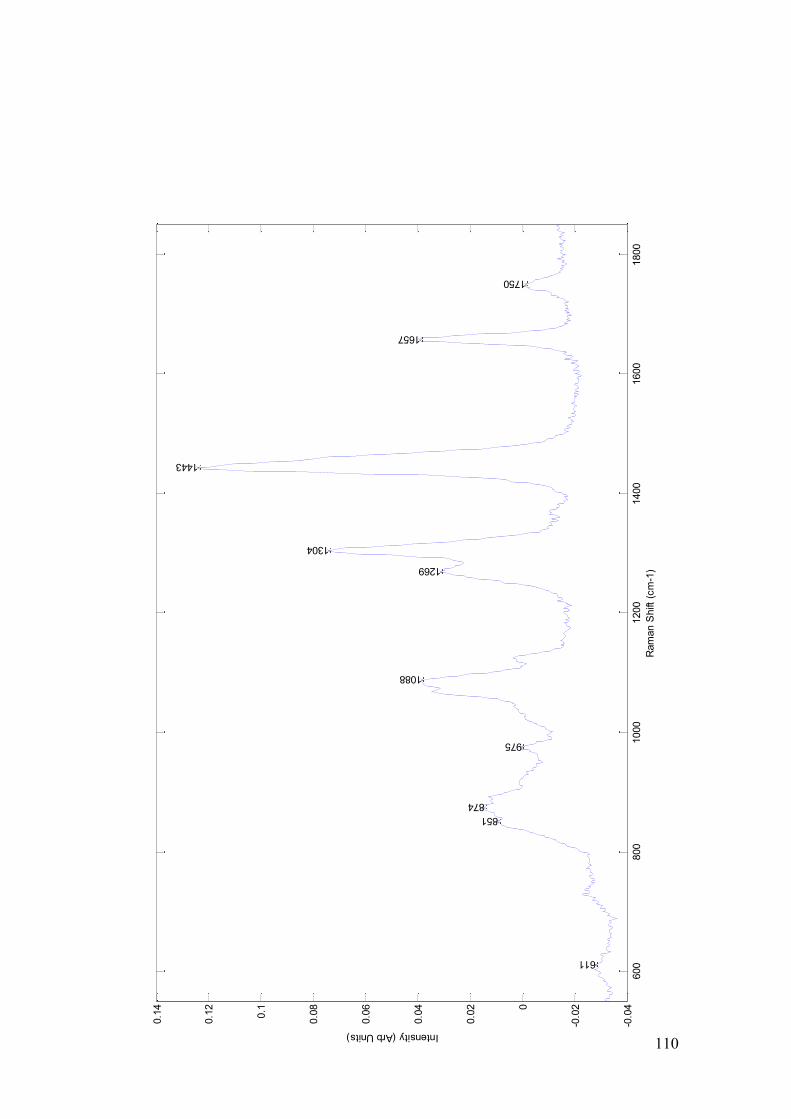
110
600
800
1000
1200
1400
1600
1800
-0.0
4
-0.0
20
0.0
2
0.0
4
0.0
6
0.0
8
0.1
0.1
2
0.1
4
Ram
an S
hift
(cm
-1)
Intensity (Arb Units)
611
874
851
975
1088
1269
1304
1443
1657
1750

111
800
900
1000
1100
1200
1300
1400
1500
1600
1700
1800
-0.0
6
-0.0
4
-0.0
20
0.0
2
0.0
4
0.0
6
0.0
8
Ram
an S
hift
cm
-1
Intensity Arb Units
1158
1530
1295
1433
1654
14651458
1671 1665
Figure 46- Spectral plot of the load for principal component 1 in the feasibility study, some peaks marked
for clarity. The contribution that this load made to the overall spectra is given by the scores (see table 8).

112
800
900
1000
1100
1200
1300
1400
1500
1600
1700
1800
-0.1
-0.0
8
-0.0
6
-0.0
4
-0.0
20
0.0
2
0.0
4
0.0
6
Ram
an S
hift
cm
-1
Intensity Arb Units
1088
1312
1447
1660
Figure 47- Spectral plot of the load for principal component 2 in the feasibility study, some peaks marked
for clarity The contribution that this load made to the overall spectra is given by the scores (see table 8).

113
Figure 48- Spectral plot of the load for principal component 3 in the feasibility study some peaks marked
for clarity. The contribution that this load made to the overall spectra is given by the scores (see table 8).
-0.06 -0.05 -0.04 -0.03 -0.02 -0.01 0 0.01 0.02 0.03 0.040
50
100
150
200
250
300
Score for PC2
Num
ber
of
spectr
a
Figure 49- Histogram plotting the scores for principal component 2 of both H and E defined negative
nodes (green) and positive nodes (red) in the feasibility study to demonstrate its ability to divide the two
groups.
In the third phase of spectral interpretation linear discriminant analysis (LDA) fed by
the principal components was used to improve the separation of the two pathological
groups by providing a supervised classification algorithm (as is explained further in
Chapter 4). In this calculation the first 25 principal components were used. The results
of this analysis revealed a sensitivity and specificity of differentiation between the two
groups of 95.7% and 98.9% respectively (Table 9) (Figure 50). This is clearly

114
comparable with many of the current methods of intra-operative analysis and strongly
supports the potential of this technology in that role.
H and E defined
Positive Nodes
H and E defined
Negative Nodes
Raman Spectra ( Positive)
1166
26
Raman Spectra (Negative)
52
2358
Sensitivity =95.7%
Specificity=98.9%
Table 9- The sensitivity and specificity achieved in the feasibility study on an individual spectral basis
using linear discriminant analysis fed by the principal components.
-0.03 -0.025 -0.02 -0.015 -0.01 -0.005 00
20
40
60
80
100
120
140
160
180
PCA fed LDA score
Num
ber
of
Spectr
a
Positive Nodes
Negative Nodes

115
Figure 50- Histogram plotting the scores for the linear discriminant analysis fed by the principal
components of both H and E defined negative (green) and positive (red) nodes in the feasibility
experiment .
The influence of each of the principal components in achieving this result were assessed
by repeating the LDA calculation with increasing numbers of PCs , starting with just
the first PC. These training results achieved a sensitivity and specificity of >90% using
only the first 8 PCs although the best results were achieved when all 25 PCs were
included (Figure 51).
In the fourth stage of spectral interpretation the strength of these findings were
scrutinised using a leave one node out validity test. Initially all spectra from one node
were removed and individual spectra projected onto the training set using 25 principal
components. This demonstrated that Raman spectroscopy was 75% sensitive and 94%
specific when differentiating between normal and metastatic tissue for this dataset. This
remains comparable to the sensitivities and specificities achieved for other intra-
operative techniques; particularly frozen section analysis and touch imprint cytology,
but a larger dataset would be expected to improve upon these results.

116
0
10
20
30
40
50
60
70
80
90
100
0 1 2 3 4 5 6 7 8 9 10 11 12 13 14 15 16 17 18 19 20 21 22 23 24 25
Principal Components
Percentage
Sensitivity
Specificity
Figure 51- Sensitivity and specificity at splitting H and E defined negative and positive nodes in the
feasibility study using increasing numbers of principal components in the linear discriminant analysis.
To help simulate acquisition of data in a time frame that was suitable for intra-operative
use the next section of analysis went on to alter the numbers of spectra from each node
that were included in the analysis. 5, 10 and 25 spectra from each node were randomly
selected from the total spectra acquired from each node. These numbers were selected
following discussions with the clinicians involved in the project. Data related to current
techniques and surgical experience suggests that there would be approximately 40
minutes per patient to process and assess all the nodes sampled. If up to 5 nodes were
sampled from each patient and divided into two then there would be less than 4 minutes
to prepare and assess each sample It was important therefore to appreciate the affect
that smaller spectral numbers would have on the results achieved.

117
A Matlab® programme was written that randomly selected 5, 10 and 25 spectra from
the total spectra sampled from each node. These were then used to create a mean
spectrum for each sample. The sensitivity and specificity of the test based on the results
of PCA fed LDA and leave one node out cross validation was then calculated based on
mean spectra containing 5, 10 and 25 spectra each (Table 10).
5 spectra per node
10 spectra per node
25 spectra per node
Sensitivity
77% (10/13)
85% (11/13)
92% (12/13)
Specificity
96% (24/25)
100% (25/25)
100% (25/25)
Table10-The sensitivity and specificity achieved in leave one node out cross validity testing using a range
of spectra per node.
In the final stage of analysis the above results from 5 spectra per node (Table 10) were
used to mimic the clinical scenario in which the system might one day be used. Of the
17 patients included in the feasibility study, 11 had a negative axilla (i.e. all nodes
negative) and 6 had at least one node positive (range 1-4). If any of these nodes
sampled were found to have evidence of metastases then an axillary node clearance
would have been recommended. Using the data presented here, 5 out of the 6 patients
who were advised to have an axillary clearance post operatively would have been
successfully identified and been able to receive the benefits of an immediate rather than
a delayed axillary clearance. One patient with a single positive node would initially
been deemed to have a negative axilla only to have this changed on post operative H

118
and E analysis. Of the 11 patients with negative axilla none would have been
recommended an axillary clearance based on the Raman results (Table 11). The only
false negative was in a node from a patient with other positive nodes. One possible
explanation for this could be that the H and E analysis had missed a metastasis which
was then picked up by the Raman analysis.
H and E defined
Positive Axilla
H and E defined
Negative Axilla
Raman Positive Axilla
5
0
Raman Negative Axilla
1
11
Sensitivity = 83%
Specificity=100 %
Table 11: The sensitivity and specificity achieved in the feasibility study at identifying positive and
negative axilla using Raman spectroscopy.
3.4.3 Experiment 2 – Conclusions.
Given the sensitivity and specificity achieved both with PCA fed LDA (supervised
testing) and leave one node out cross validation (unsupervised testing) it was felt that
these results support the potential of a hand held Raman spectroscopy device for use in
the intra-operative assessment of axillary lymph nodes. Importantly the feasibility study
also enabled one to demonstrate that equivalent results could be achieved by selecting a
smaller subset of spectra from each node. Even when only 5 spectra per node were

119
assessed the sensitivity and specificity remained consistent. Given the pressures on time
that are going to be evident when using fresh tissue in a clinical setting this is an
important concept to demonstrate. Importantly if Raman spectroscopy had been used to
guide management 5 patients would have benefited from immediate axillary surgery
and none would have been advised to have an axillary clearance that later was deemed
to be unnecessary.
3.5. Experiments 3 and 4 - Overcoming the effects of operative theatre lighting
Encouraged by the results of the feasibility study planning of an intra-operative study
using the portable probe Raman spectroscopy system continued. One of the key
problems that needed to be overcome if this was going to be possible was the effect of
theatre lighting on the spectra obtained. The first step in this process was understanding
the nature of theatre lighting. Lighting within the operating theatre includes both the
general illumination as well as the operating lights. The illumination of the surgical site
is vital to optimise the surgeon’s view of the operating field and operating lights are
therefore specifically designed to meet this goal.
The majority of operating field illumination is provided by overhead lights. These are
often white fluorescent but may also be incandescent. Whilst the level of general
illumination should be at least 200 foot candles (2095 lux) to allow the theatre staff
including the anaesthetist to work safely the surgical lights should be in the range of
2500-27,000 foot candles (26,190-290,628 lux) (Berry and Kohn 2000). These lights
need to be able to provide contrast between both tissue types and tissue depths without

120
casting shadows and focused in such a way as to avoid a dark centre. There are a wide
variety of different lights marketed by an array of different companies. Not only do the
lights in different theatres vary but the way the lights are set up and used also varies.
41% of German surgeons report that they use a single main light with a smaller satellite,
43% use two equally sized large lights and 16% use three equally sized large lights
(Matern and Koneczny 2007). Further complicating this is the preference of some
surgeons to operate with low levels of ambient or general light whilst others maintain
the general lighting throughout the procedure. Many UK hospitals have developed in
stages over a number of years with new operating suites added as the need arose. As a
result operating suites will have a variety of different theatre lights within a single
hospital.
Background lighting has an adverse effect on Raman spectroscopy as it is recorded at
intensities that swamp the low intensity of Raman scattered light. The spectral
acquisition from biological tissue is often performed in darkened laser laboratories.
Providing mechanisms to exclude background light is vital to the effective functioning
of an intra operative Raman device.
Potential solutions included switching all the theatre lights off to create a darkened
environment or applying filters to all the lights. Creating a darkened theatre was
rejected due to the potential negative consequences this may have for the patient and the
safety implications for the theatre staff. The application of filters to all the theatre lights
was considered impractical because of the variety of theatre light designs in use, as well
as the problems with infection control and the possibility of surgical site contamination

121
if the filter were to become loose. An alternative was theorised based on excluding the
light from the immediate area around the probe tip. In this way the device could be used
in all lighting conditions within the operating theatre without the potential deleterious
side effects.
3.5.1. The Light Eliminator design
The basis of the design was the standard film case used to prevent light contamination.
This was modified to allow the Raman probe to be housed within it. The design of the
probe includes a tip that ensure the optimal positioning of the matter being investigated
when it is in contact with the tip. A removable lid allows the matter to be positioned in
the correct position (Figure 52, 53).
3.5.2. Experiment 3 (The Light Eliminator Experiment, Part A) –
Methods.
The light eliminator was first tested within the operating theatres at Gloucestershire
Royal Hospitals NHS Foundation Trust. Prior to its use within this environment local
rules were designed to ensure safe use and the experiments were carried out at times
when the operating theatres were not in clinical use.

122
Figure 52 Outline design drawings for a light eliminator (not to scale)(left) and photograph of the Light
eliminator in place over the end of the probe tip(right). The probe is held facing upwards. The sterile
sheath is placed around it and the eliminator is then placed over this. The tissue can then be placed on
the central flat surface and a light resistant lid placed and secured. .
A B
Rem
ovab
le L
id –
allo
ws
easy
pos
ition
ing
of th
e sa
mpl
e at
pos
ition
A.
Pla
stic
cas
ing –
cons
truc
ted
usin
g th
e sa
me
plas
tic u
sed
to c
ase
cam
era
film
s
The
Ram
an P
robe
, mou
nted
in a
n up
right
pos
ition
Ste
rile
She
ath –
used
to
mai
ntai
n st
erili
ty
Oth
er fe
atur
es n
ot s
how
n he
re in
clud
e a
rubb
er
bung
at p
ositi
on (
B)
to a
llow
tig
ht f
ittin
g of
the
prob
e an
d lig
ht e
limin
atio
n fr
om b
enea
th th
e ca
se

123
Using the MiniRam II Raman spectrometer spectra were obtained from a standard block
of PTFE. This block measured 2cm x 1cm and was used due to its clear and
characteristic peaks. This is used as a standard measurement by the research group.
Theatre temperature was maintained at 22 ºC throughout the experiment and the laminar
ventilation system was switched off. The spectroscopy device was placed on a standard
theatre trolley in the corner of the theatre approximately 3m away from the operating
table, a position that may be mimicked when the device is used in the intra-operative
setting.
Spectra were obtained in four lighting conditions.
1. Background lights and operating lights on.
2. Background lights on and operating lights off.
3. Operating lights on and background lights off.
4. All lights within the theatre switched off.
In each of these situations 10 spectra were recorded (by combining 16 1s acquisitions)
both with and without the light eliminator device in situ. The data were transferred to a
desktop PC and analysed using Matlab® software.
3.5.3. Experiment 3 – Results.
The mean plots of spectra obtained without the eliminator demonstrated the deleterious
effects of both the background and operating lights (Figure 54). The spectra obtained
when the operating lights were on demonstrated saturation of the CCD and there were

124
multiple additional peaks in the spectrum obtained with only the general lights on.
These results confirm that both the theatre lights and the general lighting make
interpretation of the PTFE spectra either very much more difficult or impossible. Given
the relatively high intensities of the PTFE peaks it is likely that this would be replicated
or indeed made worse when using biological specimens.
The effect of the eliminator in this observational study was evident when the mean
spectra of the data were plotted for the four lighting settings both with and without it in
place (Figure 55). It was thus hoped that the light eliminator would facilitate the use of
the MiniRam II Raman spectrometer within the operating theatre. Due to the prominent
PTFE peaks further experiments were designed to assess the effect of the light
eliminator when using biological tissue.

125
Figure 54- Mean spectra (n=10) for PTFE from four lighting conditions collected in an operating theatre
to demonstrate the deleterious effects of background and operating lights.

126
400 600 800 1000 1200 1400 1600 18000
0.05
0.1
0.15
0.2
No Lights + Eliminator
400 600 800 1000 1200 1400 1600 18000
0.05
0.1
0.15
0.2
No Lights
400 600 800 1000 1200 1400 1600 18000
0.05
0.1
0.15
0.2
Background + Eliminator
400 600 800 1000 1200 1400 1600 18000
0.05
0.1
0.15
0.2
Background
400 600 800 1000 1200 1400 1600 18000
0.05
0.1
0.15
0.2
Operating Lights +Background Lights + Eliminator
400 600 800 1000 1200 1400 1600 18000
0.01
0.02
0.03
0.04
Operating Lights + Background Lights
400 600 800 1000 1200 1400 1600 18000
0.05
0.1
0.15
0.2
Operating Lights + Eliminator
400 600 800 1000 1200 1400 1600 1800-0.06
-0.04
-0.02
0
0.02Operating Lights
Figure 55- Mean spectra (n=10) for four lighting conditions both in the presence of the light eliminator
(left) and without it (right) (y axis = intensity AU and x axis = Raman Shift cm-1
).

127
3.5.4. Experiment 4 (Light Eliminator Experiment Part B) – Methods.
To determine the effect of the eliminator when obtaining spectra from biological tissue
the device was tested within the laser laboratory using axillary lymph node tissue rather
than PTFE. A single lymph node that had been collected and stored as part of the
feasibility study was used. This node was not included in the feasibility study but its
handling both at the time of collection and during the experiment was a described in
Chapter 3.4. Standard laboratory conditions were maintained except for the switching
on of all the lights as required by the experiment.
16 x 1 second acquisitions were used to collect 5 spectra from the node using the
MiniRam II Raman spectrometer. These were obtained in the following conditions;
Standard laboratory conditions (all lights off).
Standard conditions with lights on.
Standard conditions with lights on and using the eliminator device.
The data was then transferred to a standard desktop PC and interpreted using Matlab ®
software. Principal component analysis, ANOVA analysis and Student’s t-tests were
used to assess the results.

128
3.5.5. Experiment 4 – Results.
Examination of the resulting spectra demonstrated that the spectra obtained in standard
laboratory conditions were markedly different to the spectra obtained with the lights on.
As expected the spectra obtained with the lights on, but without the eliminator, were
overwhelmingly dominated by peaks resulting from the laboratory lights (Figure 56).
The spectra obtained with the eliminator in place appeared very similar to the spectra
obtained under standard laboratory conditions. There were differences in intensity and it
was felt that this may represent the different orientation of the node which had been
repositioned during the experiments (Figure 57a).
The principal components of the three sets of spectra were then calculated using self
built programmes in Matlab®. An ANOVA calculation was performed on the scores of
each principal component to determine which the most significant principal components
were. PC 1 and 2 were calculated to have f values of 110686 and 115 respectively. The
loads that pertained to these PCs were plotted and it was evident from inspection of
these plots that PC1 related to that of the laboratory lights and that PC2 related to that of
the lymph node spectra (Figure 58).
When the scores for PC1 were plotted it could be seen that the eliminator had been
successful at eliminating the light as the scores for both the spectra taken with the light
turned off and those taken with the lights on were very similar (Figure 59).

129
400
600
800
1000
1200
1400
1600
1800
0.0
05
0.0
1
0.0
15
0.0
2
0.0
25
0.0
3
0.0
35
0.0
4
0.0
45
0.0
5
0.0
55
Ram
an S
hift
(cm
-1)
Intensity (normalised Arb Units)
Lym
ph n
ode s
pectr
a u
nder
dark
labora
tory
conditio
ns
400
600
800
1000
1200
1400
1600
1800
0
0.0
2
0.0
4
0.0
6
0.0
8
0.1
0.1
2
0.1
4Lym
ph n
ode s
pectr
a w
ith labora
tory
lig
hts
on
Figure 56- Mean spectra collected from an axillary lymph node (n=5) under standard laboratory
conditions and with lights on.

130
200
400
600
800
1000
1200
1400
1600
1800
2000
0.0
05
0.0
1
0.0
15
0.0
2
0.0
25
0.0
3
0.0
35
0.0
4
0.0
45
0.0
5
0.0
55
Ram
an S
hift
(cm
-1)
Intensity (Arb Units)
Node in L
abora
tory
conditio
ns
200
400
600
800
1000
1200
1400
1600
1800
2000
0.0
05
0.0
1
0.0
15
0.0
2
0.0
25
0.0
3
0.0
35
0.0
4
0.0
45
0.0
5
0.0
55
Node in L
abora
tory
with lig
ht
on +
Elim
inato
r
Figure 57- Mean spectra (n=5) collected from an axillary lymph node under standard laboratory
conditions and with the laboratory lights on with the light eliminator.

131
400
600
800
1000
1200
1400
1600
1800
-0.0
4
-0.0
20
0.02
0.04
0.06
0.080.1
Ram
an S
hift
(cm
-1)
Intensity (arb Units)
Load
s fo
r P
C1
400
600
800
1000
1200
1400
1600
1800
-0.1
2
-0.1
-0.0
8
-0.0
6
-0.0
4
-0.0
20
0.02
0.04
0.06
Load
s fo
r P
C2
Figure 58- Spectral plots of the loads for principal components (PC) 1 and 2 in experiment 4. PC1
appears to be representative of the laboratory lights and PC2 resembles the spectra that are obtained
from an axillary lymph node.
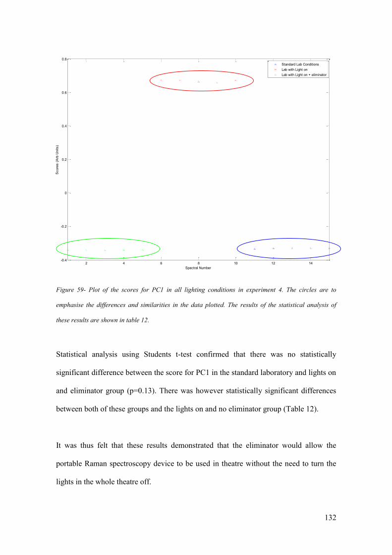
132
2 4 6 8 10 12 14-0.4
-0.2
0
0.2
0.4
0.6
0.8
Spectral Number
Score
s (
Arb
Units)
Standard Lab Conditions
Lab with Light on
Lab with Light on + eliminator
Figure 59- Plot of the scores for PC1 in all lighting conditions in experiment 4. The circles are to
emphasise the differences and similarities in the data plotted. The results of the statistical analysis of
these results are shown in table 12.
Statistical analysis using Students t-test confirmed that there was no statistically
significant difference between the score for PC1 in the standard laboratory and lights on
and eliminator group (p=0.13). There was however statistically significant differences
between both of these groups and the lights on and no eliminator group (Table 12).
It was thus felt that these results demonstrated that the eliminator would allow the
portable Raman spectroscopy device to be used in theatre without the need to turn the
lights in the whole theatre off.

133
Comparison
Mean for the score of PC1 in each group
(n=5)
(SD and SEM)
p value
Standard laboratory conditions
v.
Lights on (no eliminator)
0.349 (0.001, 0.00045)
v
0.661 (0.004, 0.002)
p<0.0001
Standard laboratory conditions
v.
Lights on (with eliminator)
0.349 (0.001, 0.00045)
v.
0.347 (0.005,0.001)
p= 0.1303
Lights on (no eliminator)
v.
Lights on (with eliminator)
0.661 (0.004, 0.002)
v.
0.347 (0.005,0.001)
p<0.0001
Table 12: A comparison of the mean score (n=5) for PC1 in each of the three lighting conditions in
experiment. The results of statistical analysis, using a Student’s t-test, to compare these results are shown
(SD= standard deviation, SEM= standard error of the mean).
3.6. Experiment 5 -Effect of theatre temperature variations.
Having determined an effective way of overcoming the effects of theatre lighting the
next variable that needed to be explored was that of temperature variations within the
operating theatre. Previous work using Raman spectroscopy to assess axillary lymph
nodes has been carried out in a laser laboratory where the temperature was regulated to
remain at 21ºC. The ambient temperature of an operating theatre may vary as a result of
the need to maintain the patient’s temperature throughout an operation. The importance
of altering the theatre temperature is demonstrated by figures that suggest that up to
70% of patients may experience a degree of inadvertent hypothermia during an

134
operative procedure (Burger and Fitzpatrick 2009). Not maintaining a suitable ambient
temperature within the operating theatre was one of the key factors linked to this
inadvertent hypothermia (Young and Watson 2006).
A review of the literature pertaining to ambient temperature published in 2006
suggested that an ambient temperature of at least 22°C should be maintained with some
authors suggesting temperatures of up to 26°C (Young and Watson 2006). The
importance of maintaining the balance between the patient’s core temperature and the
ability of the surgical team to operate is recognised by the authors especially as the
temperature rises above 22°C. Most surgeons prefer to operate at temperatures between
18.5 and 22°C (Brock 1975). American guidelines for the prevention of surgical site
infection published in 1999 suggest a slightly higher ambient temperature of between
68-73°F (20-23°C) (Mangram et al. 1999). Given these competing interests it may be
that ambient theatre temperature would vary both throughout a single operation and
across different days.
3.6.1. Experiment 5 – Methods.
This experiment investigated the effects of varying the temperature across a range of
18-28°C so as to over represent the anticipated ambient temperature range that intra
operative spectral analysis would take place within. All experimental measurements
were recorded within a laser safe laboratory which has a temperature control facility
that allowed the room to be both cooled and heated. The instrumentation within this
system allowed both the room temperature to be selected and then monitored to

135
maintain the desired setting. The temperature of the room is normally set at 21°C.
Spectra of cyclo-hexane were obtained across the seven temperatures starting at 18°C
and rising in 2°C intervals to reach 28°C. The temperature within the room reached the
new temperature setting within 15 minutes. A period of 30 minutes was allowed
between temperature alterations to ensure that a stable temperature had been achieved.
All other factors within the room were kept stable. Five spectra of cyclohexane were
recorded at each of the six temperature settings. Data analysis was performed using
Matlab® mathematical software. The statistical significance of any observed differences
was tested using ANOVA analysis.
3.6.2. Experiment 5 – Results.
Inspection of the mean spectra for each temperature revealed very few changes. As
expected for cyclohexane four very distinct peaks were visible in the range of 750-1500
cm-1
(Figure 60). The position of each of the 4 most prominent peaks (labelled in Figure
60) were recorded to ensure there was no peak position drift over the temperature range
(Figure 61).
To assess the mean peak position at 6 different temperatures ANOVA, a statistical test
that simultaneously compares two or more means, was employed to determine the
statistical significance of the small shifts that had been observed. In this test the null
hypothesis was that there was no difference between the peak positions at the six
different temperature points. Using standard tables the critical “f” value at which the
null hypothesis would be rejected can be calculated.
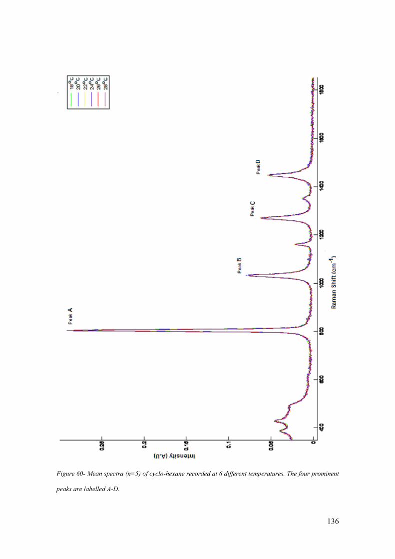
136
Figure 60- Mean spectra (n=5) of cyclo-hexane recorded at 6 different temperatures. The four prominent
peaks are labelled A-D.

137
Figure 61- Mean peak position (n=5) of the 4 cyclo-hexane peaks (labelled in Figure 60) across the
temperature range 18 -28ºC).
The position of peak A was the only one that recorded an f value greater than the critical
value. The relative peak positions of the 4 peaks were then calculated. The null
hypothesis that there was no difference between the relative positions of the 4 main
peaks at the level of p<0.01 was not rejected in any of the calculations (Table 13).
This data demonstrated that across a range of temperatures, that correlate with those
found in the operating theatre, the positions of each of the four main cyclo-hexane peaks
did not significantly differ in relation to each other. Indeed the position of peak A,
(ºC)
1 2 3 4 5 6800
802
804
806
808
810
Temp Reading 1=18, 2=20, 3=22, 4=24, 5=26. 6=28
Peak P
ositio
n (
cm
-1)
Peak A
1 2 3 4 5 61030
1032
1034
1036
1038
1040
Peak B
1 2 3 4 5 61265
1270
1275
Peak C
1 2 3 4 5 61445
1450
1455
Peak D
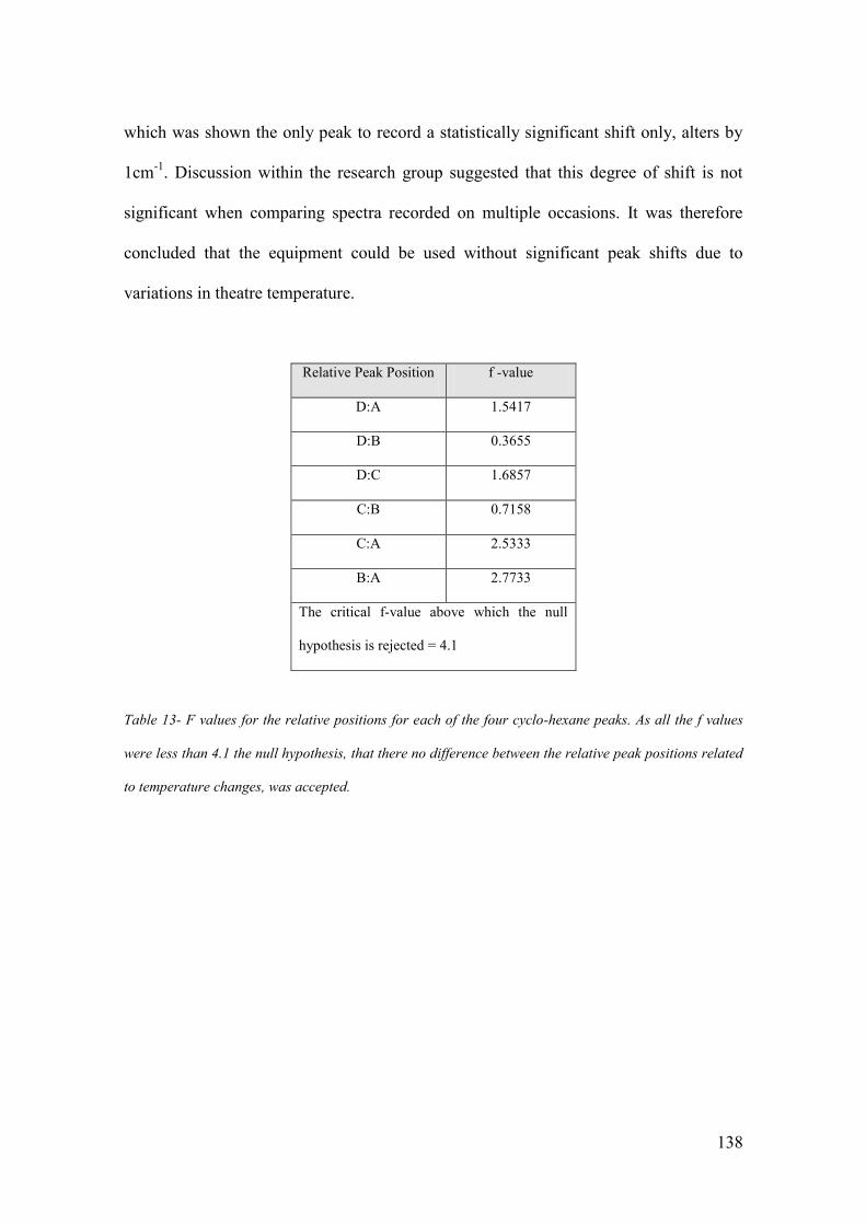
138
which was shown the only peak to record a statistically significant shift only, alters by
1cm-1
. Discussion within the research group suggested that this degree of shift is not
significant when comparing spectra recorded on multiple occasions. It was therefore
concluded that the equipment could be used without significant peak shifts due to
variations in theatre temperature.
Relative Peak Position f -value
D:A 1.5417
D:B 0.3655
D:C 1.6857
C:B 0.7158
C:A 2.5333
B:A 2.7733
The critical f-value above which the null
hypothesis is rejected = 4.1
Table 13- F values for the relative positions for each of the four cyclo-hexane peaks. As all the f values
were less than 4.1 the null hypothesis, that there no difference between the relative peak positions related
to temperature changes, was accepted.

139
3.7. Experiment 6 - Maintaining Sterility.
One of the significant concerns of the surgeons involved with this study was the need to
maintain sterility particularly if the device was to be used in an intra-operative setting.
This is of course vital to ensure there is no cross contamination from one lymph node to
the next as this could lead to false results. Further to this it is anticipated that in the
long term the device will be held by the operating surgeon possibly with the node in
situ. It must therefore also remain sterile to prevent cross contamination of the operative
field.
3.7.1. Experiment 6 – Methods.
To meet the requirement for sterility a sterile sheath that is designed for use with a hand
held ultrasound probe was identified. The JAD01 ultrasound cover (Jade Medical, RG8
9EX, UK) was used as it was readily available and due its primary purpose had a design
that was easily adapted for the Raman probe. It is made of latex free polyurethane and
measures 6 x 33 inches (Figure 62).
The sheath was placed over the whole Raman probe and secured in place with sterile
rubber bands that are supplied in each pack. The light eliminator was then placed over
the top of this. Any material being measured is only in contact with the sterile sheath.
An added advantage of mounting the sheath in this way was that small nodes could be
placed over the aperture of the inverted probe spacer without risk of them falling though
into the space above the probe tip.

140
Figure 62- The JAD01 sterile sheath used in experiment 6.
Spectra (made up of 16 x 1sec. acquisitions) were obtained from a standard block of
PTFE using the B&W Tek MiniRam II within a laser laboratory. The first ten spectra
were obtained under standard conditions and the second 10 spectra were obtained with
the sterile sheath in place (Figure 63). Data were transferred to a standard desk top PC
and interpreted using Matlab® software. ANOVA statistical analysis was then
performed to assess the positions of the 4 most prominent peaks in the PTFE spectra.
A further study was set up to ensure that there was no variation between the use of
different sheaths as it was envisaged that a separate sheath would be used for each
patient. 5 spectra were acquired from the same standard block of PTFE with the sheath
in place. This was repeated with 10 different sterile sheaths from two different batches.
Data interpretation took place using Matlab® software.

141
3.7.2. Experiment 6 – Results.
Analysis of the data from the first part of the study, using ANOVA, revealed no
statistically significant shift in the PTFE peaks. There were no additional peaks present
in the spectra obtained whilst using the sterile sheath. Similarly analysis of the 50
spectra collected in the second part of the experiment revealed that there was no
significant shift in the position or intensity of the 4 most prominent PTFE peaks
(labelled A, B, C, and D in Figure 63). Further there was no additional peaks evident for
any of the 10 different sheaths used.
It was thus concluded that the sterile sheath had little or no effect on the spectra
collected. It would therefore be used throughout the intra operative work and to
maintain sterility and avoid cross-contamination it would be changed after each patient.
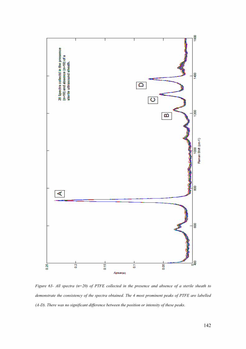
142
Figure 63- All spectra (n=20) of PTFE collected in the presence and absence of a sterile sheath to
demonstrate the consistency of the spectra obtained. The 4 most prominent peaks of PTFE are labelled
(A-D). There was no significant difference between the position or intensity of these peaks.

143
3.8. Experiments 7 and 8 -The effect of Patent V Blue Dye.
A critical part of the SLNB procedure is the correct identification of the axillary sentinel
node. As has been described, the identification of the node involves a combination of a
radio-labelled colloid and a visible dye. Locally a combination of technetium99m
labelled colloid and Patent V blue dye is used as per the national guidelines
(Somasundaram, Chicken and Keshtgar 2007). Previous work has demonstrated that the
presence of marker dyes used to orientate samples saturated the spectra obtained (Smith
2005). At that time sentinel node biopsy was not being performed routinely and the
nodes used in that study had not been exposed to blue dye. Given that the use of Patent
V blue dye is a standard part of the procedure it was vital to assess the effect that its
presence would have on the spectra that we obtained.
3.8.1. Experiment 7 – Methods.
Samples of the Patent V Blue Dye (2.5%) (Guerbet, Roissy, France) routinely used in
SLNB were obtained. There is no published data documenting the concentration of the
blue dye within the axillary lymph node itself after it passes from the breast down the
lymphatic channels. Clinically surgeons refer to the nodes on an analogue scale of 0-3
dependent on the degree of “blueness” of the excised node. The only previous work
which estimated the concentration of dye in breast tissue reported a concentration of
0.08% of methylene blue in the tissues after injection of 0.1 ml of 1% of this dye
(Hirsch et al. 1989). It is likely that the concentration of blue dye will be further diluted
by the time it reaches the lymph node. Given that there was no definitive data

144
documenting the concentration of blue dye within the node experiments were planned
that used concentrations greater than and including 0.08%.
To help determine the effect of this blue dye an experiment involving thirty 1cm3
cubes
of chicken breast (Tesco, UK) that had been dissected to mimic the size of a newly
excised lymph node was set up. The 2.5% Patent V Blue Dye was diluted using Water
for Injection (Baxter, Newbury, UK) to 1.25%. 0.63%, 0.31%, 0.16%, and 0.08%. Five
chicken cubes were placed in a tube containing 10 mls of one of the five solutions and a
further five cubes were placed in 10 mls of water for injection. These tubes were then
left at room temperature for a period of 24 hours. At the end of this period the chicken
cubes were removed from the tubes and placed on a new Petri dish.
9 spectra were obtained from each of the 30 chicken cubes using the same technique as
for axillary lymph nodes described in Chapter 4. The spectra were then transferred to a
desktop PC and interpreted using Matlab® software. Principal component analysis and
ANOVA was used to assess the differences between the different blue dye
concentrations and the controls. An unpaired t-test was used to determine the statistical
significance of the differences in the PC scores between the groups.
3.8.2. Experiment 7 - Results.
A total of 270 spectra were included in data interpretation. The mean spectra (n=45) for
the different concentrations of blue dye were calculated and compared to spectra of blue
dye previously published (Stropp et al. 2003) (Figure 64). Analysis of this spectrum,

145
obtained with an excitation wavelength of 514.5nm using surface enhanced Raman
spectroscopy techniques, revealed significant peaks at 1210 cm-1
, 1432 cm-1
and 1620
cm-1
. Similar peaks were observed in the spectra recorded from the chicken samples that
had been prepared in Patent V blue dye (Figure 64). Analysis of the spectra obtained
from the controls without the presence of blue dye was characteristic of that from
chicken breast with three evident peaks at 1328, 1455 and 1660 cm-1
( Beattie et al.
2006; Beattie et al. 2007) .
Following principle component analysis statistical testing using ANOVA calculations
revealed that the first principal component was the most significant at differentiating
between those spectra obtained in the presence of blue dye and those without ( f value
>1700). The scores obtained for the first principal component were plotted and showed
a clear difference between the two groups (Figure 65). This was confirmed with
statistical analysis (Table 14).
Mean value (and SD and SEM) of the
score for PC1 (all blue dye concentrations)
(n=225)
Mean Value (and SD and SEM) of the score
for PC1 (all controls)
(n=45)
p Value
-0.0359
(0.0121, 0.0008)
0.1673
(0.015, 0.0022)
<0.0001
Table 14: The mean value for the score of PC1 in experiment 7 in samples exposed to blue dye v controls.
The difference was highly statistically significant using an unpaired t-test. .

146
Figure 64- Mean spectra (n=45) obtained from 1 mm3 chicken breast after 24hours in 5 concentrations
of Patent V blue dye (right) compared to published spectra for patent V blue dye (left) (Stropp et al.
2003).

147
Figure 65- Histogram plotting the score for PC1 for all spectra (n=270) in experiment 7. This
demonstrates the clear separation of the scores for PC1 between the controls (red, n=45) and those
exposed to blue dye (green, n=225).
Analysis of the load associated with this principal component was very similar to that
obtained from the control chicken cubes (Figure 66). This data suggested that all the
spectra obtained in the presence of the blue dye were representative of the dye alone and
this masked the spectral features of the underlying chicken breast. This would have a
hugely detrimental effect on the proposed study as in the presence of blue dye the
underlying spectral features of the tissue might be lost and any spectral differences seen
in the tissue itself would be difficult to appreciate.
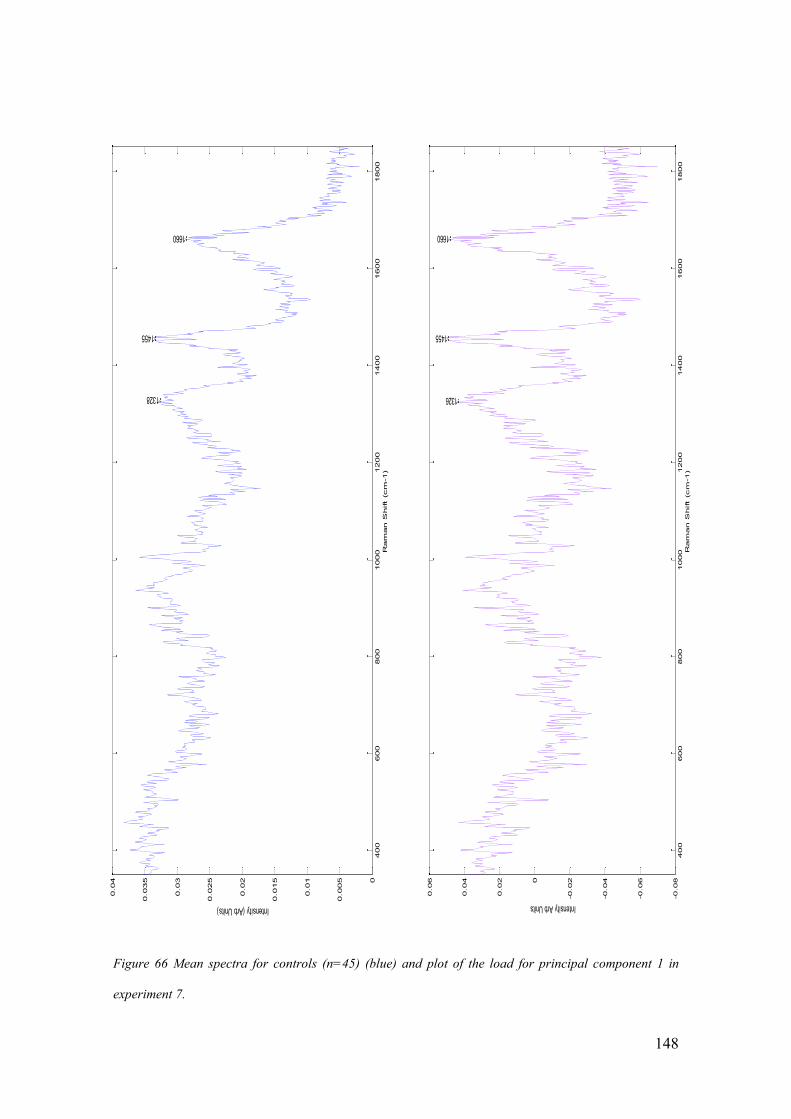
148
400
600
800
1000
1200
1400
1600
1800
0
0.005
0.01
0.015
0.02
0.025
0.03
0.035
0.04
1660
1455
1328
Ram
an S
hift (cm
-1)
Intensity (Arb Units)
400
600
800
1000
1200
1400
1600
1800
-0.08
-0.06
-0.04
-0.020
0.02
0.04
0.06
1660
1455
1326
Ram
an S
hift (cm
-1)
Intensity Arb Units
Figure 66 Mean spectra for controls (n=45) (blue) and plot of the load for principal component 1 in
experiment 7.
149
These data cast significant doubt on the validity of Raman spectroscopy at
differentiating between abnormal and normal lymph nodes in the presence of blue dye.
However the method of preparation of the tissue in this experiment is very different to
the processes which would transport the blue dye to the lymph node in vivo. It may be
that the spectral features related to the blue dye on the surface of the chicken specimens
rather than that which had diffused into the chicken tissue itself. This situation would
not occur in the lymph node where the blue dye will arrive via the lymphatic system and
then percolate its way through the node.
3.8.3. Experiment 8 – Methods.
Further studies to investigate this effect were evidently required. The results of the
feasibility study were therefore reviewed to assess the affect of the patent V blue dye
used (further details of the methodology of collecting and assessing the lymph nodes
are contained in Chapter 3.4). In the feasibility study 11 nodes had been acquired during
a sentinel lymph node biopsy and 27 had been collected during an axillary dissection.
As part of the standard SLNB procedure the “blueness” of the node is recorded after it
is excised from the patient. All the nodes in the feasibility dataset were rated on an
analogue scale of 0 to 3 by the lead surgeon at the time of surgery (0 = no blue, 1 =
faint blue, 2 = moderate blue and 3 = strong blue). It was therefore possible to create a
dataset that included nodes that had no exposure to blue dye at all and those with
visually increasing concentrations of blue dye (Table 15). In addition to this 60 spectra
were obtained, by the same methodology, from standard samples of 2.5% Patent V blue
dye (Guerbet, Roissy, France). All the spectra were assessed using Matlab® software.

150
Principal component analysis was performed along with ANOVA statistical testing to
determine which of the principal components was statistically most significant at
differentiating between the groups. The statistical significance of the difference in the
mean scores for this PC was then confirmed using an unpaired t-test.
Blueness of Node Number of Nodes Number of Spectra
0
27
2448
1
4
394
2
3
291
3
4
391
Table 15- Numbers of nodes and total spectra in each group in experiment 8 (blueness measured at the
time of surgery by the operating surgeon; 0 = no blue on visual inspection or not exposed to it, 1 = faint
blue, 2 = moderate blue and 3 = strong blue) .
3.8.4. Experiment 8 – Results.
A total of 3584 spectra were included in the dataset. Principal component analysis was
performed on the dataset to identify the principal component that was associated with
blue dye. The statistical significance of each of the PCs in differentiating between the
four different node groups and the blue dye was determined using ANOVA statistical
calculations. Principal component 2 was the most statistically significant with an f value

151
of 2103. The plot of this PC closely resembled the mean spectra of Patent V blue dye
with peaks at 1165,1219,1288 and 1610cm-1
being present in both plots (Figure 67).
Examination of the mean scores for each group supports PC2 as the PC associated with
the blue dye. This is firstly because the mean score for the pure dye spectrum is very
positive and secondly that the mean score increases as the “blueness” of the nodes
increases (Figure 68) (Table 16). The differences between the mean scores were then
assessed using an unpaired t-test (Table 17).
Group
Total Number of
Spectra
Mean score for PC2
(standard deviation and standard
error of the mean)
Blue dye score 0
2448
-0.0070
(0.015,0.0003)
Blue dye score 1
394
-0.0083
(0.014, 0.0007)
Blue dye score 2
291
-0.0054
(0.01, 0.0006)
Blue dye score 3
391
0.0004
(0.006,0.0003)
Patent V blue dye 2.5%
60
0.14
(0.0008, 0.0001)
Table 16 - Mean value for the score of PC2 in the 5 groups in experiment 8. Standard deviation and
standard error of the mean are also shown (blueness measured at the time of surgery by the operating
surgeon ; 0 = no blue or not exposed to blue dye, 1 = faint blue, 2 = moderate blue and 3 = strong blue).

152
Figure 67- Mean spectra (blue, left) of Patent V blue dye (n=60) and the load of PC2 (red, right) in
experiment 8 with the distinct similarities between the two highlighted.

153
Figure 68- Mean score with standard error bars for PC2 in experiment 8 in the five separate groups
across the range of blueness (blueness measured at the time of surgery by the operating surgeon ; 0 = no
blue (or not exposed to blue), 1 = faint blue, 2 = moderate blue and 3 = strong blue)(for numbers in each
group see table 15).
Groups being compared P value (unpaired t-test)
0 v 1 0.107
0 v 2 0.076
0 v 3 p<0.001
0 v 4 p<0.001
1 v 2 0.002
1 v 3 p<0.001
1 v 4 p<0.001
2 v 3 p<0.001
2 v 4 p<0.001
3 v 4 p<0.001
Table 17: Statistical significance of the differences in the mean value for the scores of PC2 between each
group using an unpaired t-test in experiment 8. (Group 0 = No dye, group 1= faint blue, 2=moderate
blue, 3 = strong blue and 4=Patent V blue dye 2.5%).

154
None of the loads for the other principal components appeared to have peaks suggestive
of blue dye. Further they were neither as statistically significant using ANOVA analysis
or displayed the same change in mean score as was demonstrated for PC2. This
principal component was thus deemed to most closely represent the contribution of blue
dye.
To assess the effect of this component on the ability of the system to differentiate
between the different pathologies PCA fed LDA was performed both in the presence of
and in the absence of this PC. When PC fed LDA was calculated for all the scores
trained on gold standard histopathology results the sensitivity and specificity of the
Raman system at differentiating between cancer and normal tissue was 95.7% and
98.9% respectively as discussed previously. When the same calculation was performed
using all the scores except for that from PC 2 the sensitivity and specificity remained
virtually unchanged at 95.1% and 99.6%.
Given these results it was felt, despite the results of experiment 7, that the presence of
blue dye of varying concentrations would have little effect on the spectra obtained.
Indeed further it does not significantly adversely affect the ability to differentiate
between normal and metastatic lymph nodes.

155
4. Intraoperative Analysis of Axillary Lymph Nodes
Having demonstrated that the Mini Ram II could be used within the operating theatre
context to differentiate between positive and negative nodes the next phase of the
project moved onto using the equipment within the operating theatre, on freshly excised
tissue, in real time. Prior to embarking on this phase both ethical and laser safety
approval needed to be achieved.
Ethical approval was granted by the Gloucestershire Local Ethics Committee (approval
code 01/158G – “The Development of Raman Spectroscopy in the Diagnosis of Breast
Cancer”). Patients were eligible for inclusion in the study if they had a diagnosis of
breast cancer and were undergoing lymphatic surgery as part of the management of this
condition. Patients were excluded from the study if they were unable to give informed
consent. A leaflet explaining the nature of the study was distributed to eligible patients
at the time of their pre-admission clinic. Consent forms were signed by all patients who
agreed to take part in the study prior to the operative procedure. As involvement in the
study did not change patient management in any way recruitment was fairly
straightforward and well received by patients.
To satisfy laser safety requirements the portable Mini Ram II system was used in a
room situated next to the operating theatre. This room was chosen as it was both
windowless and had a lockable door. It was deemed that despite the relative safety of
the laser within the spectrometer this location would further mitigate against potential
risk. Whilst in the future it is hoped that the tissue will be assessed and thus remain in

156
the operating theatre it was felt that this was a suitable interim step during the evolution
of the technique.
4.1. Materials and Methods
Axillary lymph nodes were analysed in the study from patients who were undergoing
either a sentinel lymph node biopsy (SLNB) or an axillary clearance. Samples were
obtained from a total of 72 operative procedures (57 SLNB and 15 axillary clearances).
6 patients had nodes assessed during both an initial SLNB and a subsequent axillary
clearance. Thus 66 individual patients were included in this phase of the study. Of these,
55 (83%) had an invasive ductal carcinoma of the breast, 6 had lobular carcinoma, 2 had
mucinous tumours, 1 had a tubular adenocarcinoma, 1 had a metaplastic tumour and 1
was having a SLNB because of extensive DCIS. Of the 55 patients with invasive ductal
carcinoma 23 (42%) had grade III disease, 27 (49%) had grade II disease and 5 (9%)
had grade I disease. These numbers were broadly consistent with the UK population as
discussed in Chapter 1.
19 (29%) patients included in the study had lymph nodes positive for either
macrometastases (n=13) or micrometastases (n=6). 15 of these patients had their
positive nodes discovered following SLNB and 4 had received preoperative diagnosis
following an USS and core biopsy. A total of 176 axillary lymph nodes were assessed
during the 72 operative procedures. To minimise the risk of nodes being assigned to the
wrong patient all analysis was performed before another patient entered theatre. Prior to
spectral analysis nodes were cleared of surrounding fat and cut into two equal halves. If
157
the node was too small for this to be done easily then the node was measured as a whole
node. This occurred in 13 cases and in all cases the maximum diameter of the node was
5 mm. As a result 339 samples were assessed. All samples were assessed post
operatively by standard histopathological protocols. Nodes sampled during SLNB were
cut at 2 mm intervals and underwent H and E and immuno histochemistry staining.
Nodes sampled during axillary clearance were cut in two planes and exposed to H and E
staining only. Histopathology classification was provided for each separate node
sample.
In the clinical context of deciding further treatment for each patient included in the
study the node was assessed based on the results from both halves of the node. Thus the
overall status of a node with a macrometastases in only one half was macro metastasis
positive. However within the context of this study the results from each separate node
half were used.
Of the 176 nodes assessed, 139 were defined as negative on histological examination,
18 were positive for macrometastases, 5 were positive for micrometastases, 8 were
positive for ITCs and 6 samples were reported as having no lymphoid tissue present
within the sample (Table 18). When the node halves were examined, 276 were negative,
32 were positive for macrometastases, 8 were positive for micro metastasis, 10 were
positive for ITCs and 13 had no evidence of lymphoid tissue present (Table 18). The
negative halves were further sub-divided into 160 that were from patients who had no
other positive nodes, N0 patients, or 116 that were from patients who had at least one
other positive node.

158
Number of Nodes Number of separate tissue samples
(either halve a node or a whole small node)
Negative
139
276
Positive – Macro
18
32
Positive – Micro
5
8
ITCs
8
10
Non Lymphoid
6
13
Table 18- The number of samples and nodes in each classification group. The whole nodes were
classified according to their highest group ( i.e. a node which had a macrometastases in one halve and
an ITC in the other half was classified as a macrometastases) and the halve node samples were classified
according to their halve only. The majority of nodes were divided into two halves. However due to their
small size 13 nodes were assessed as a whole.
4.1.1. Spectral Acquisition.
After excision and preparation each node was placed on the upturned probe. Prior to
assessment, a sterile sheath had been placed over the probe tip to prevent cross
contamination. The node was placed in an approximately central position and spectra
were obtained by combining 16 1s acquisitions. A total of 2627 spectra were collected
from the 339 samples. (Mean 7.2 spectra per node, range 5-25 per sample). Once
collected, spectral data was uploaded into Matlab® for spectral analysis.
159
Three standard spectra were collected during each session as is routine within the
research group. Standard spectra were obtained from a green glass standard,
cyclohexane, and a plastic pipette tip. Data was stored within a password protected
database that recorded patient details, the type of tumour, hospital number, the date of
surgery, the operating surgeon, the surgical procedure, the size of the node and the final
pathology data.
4.1.2. Spectral Analysis.
Spectra were collected from the lymph node samples at the time of surgery as described
previously. No spectra were removed during data processing as any spectra that were
either saturated or contained cosmic rays were identified and removed during collection.
Each spectrum was subjected to a stepwise sequence of processing. Initially all raw
spectra (Figure 69) were corrected for peak position and intensity. This was performed
using in house Matlab® functions and based on the calibration standards that were
recorded at the start of each session (Figure 70). Peak position calibration was first
performed based on the peak positions of the four highest intensity Cyclohexane peaks.
The Matlab® programme used cropped the spectra to 400-1800cm-1
. The resulting
spectra were then intensity corrected based on the spectra recorded from the green glass
standard.

160
Figure 69 – Raw spectra collected from all lymph node samples in the intra-operative series (n=2627).
This demonstrates the wide range of background intensity of the samples collected.

161
200 400 600 800 1000 1200 1400 1600 1800 20000.012
0.014
0.016
0.018
0.02
0.022
0.024
0.026
0.028
0.03
0.032
Raman Shift (cm-1)
Inte
nsity
600 700 800 900 1000 1100 1200 1300 1400 1500 16000
0.05
0.1
0.15
0.2
0.25
Inte
nsity
Raman Shift (cm-1)
Figure 70 – Raw spectra for green glass (above) and cyclohexane (below) standards obtained in the
Cheltenham series demonstrating the stability of the system over the course of the study (y axis intensity
is arbitrary units).

162
Following these steps the spectra were baseline corrected, smoothed and finally
normalised using in house and self programmed Matlab® functions. A mean spectrum
was then calculated for each of the nodes analysed (Figure 71).
Figure 71– Mean corrected spectra for all node samples (n=339) in the intra-operative study.
Using this methodology a dataset that pertained to the 339 samples was created that had
been corrected in a uniform and consistent way. This dataset was organised so that it
could easily be manipulated based on individual patients, node pathology or date of
spectral acquisition. This was referred to the “overall dataset” and separate pathology
subgroups and sub-datasets were created from it.
163
4.2. Results - Dataset 1: Macrometastases v. Negative N0 Nodes.
Of the five pathology groups identified from the histopathology results the two with the
greatest histopathological differences were the groups that were identified as containing
macrometastases (n=32) and the group that were defined as negative nodes from N0
patients (n=160). It was anticipated that the spectral differences between these groups
would be the most significant. Initial comparison of the spectra for these two subgroups
was performed after calculating the mean spectra for each one (Figure 72).
Significant areas of difference were evident simply on inspection of the mean spectra
and this was emphasised by plotting the mean spectra with 95% confidence intervals
either side of the mean value for each wavenumber (Figure 72, 73). This change was
enhanced when we subtracted the mean positive spectra from the mean negative spectra.
A plot of the result of this manipulation for each wavenumber gave further clarity to the
distinct differences (Figure 74). Those peaks that remained positive were representative
of increased relative concentrations within the N0 node subgroup and those peaks that
were negative indicated increased relative concentration within the macrometastases
subgroup of nodes.

164
Figure 72 – Mean spectra of NO Nodes (green, n=160) and macrometastases (red, n=32) in the intra-
operative study.
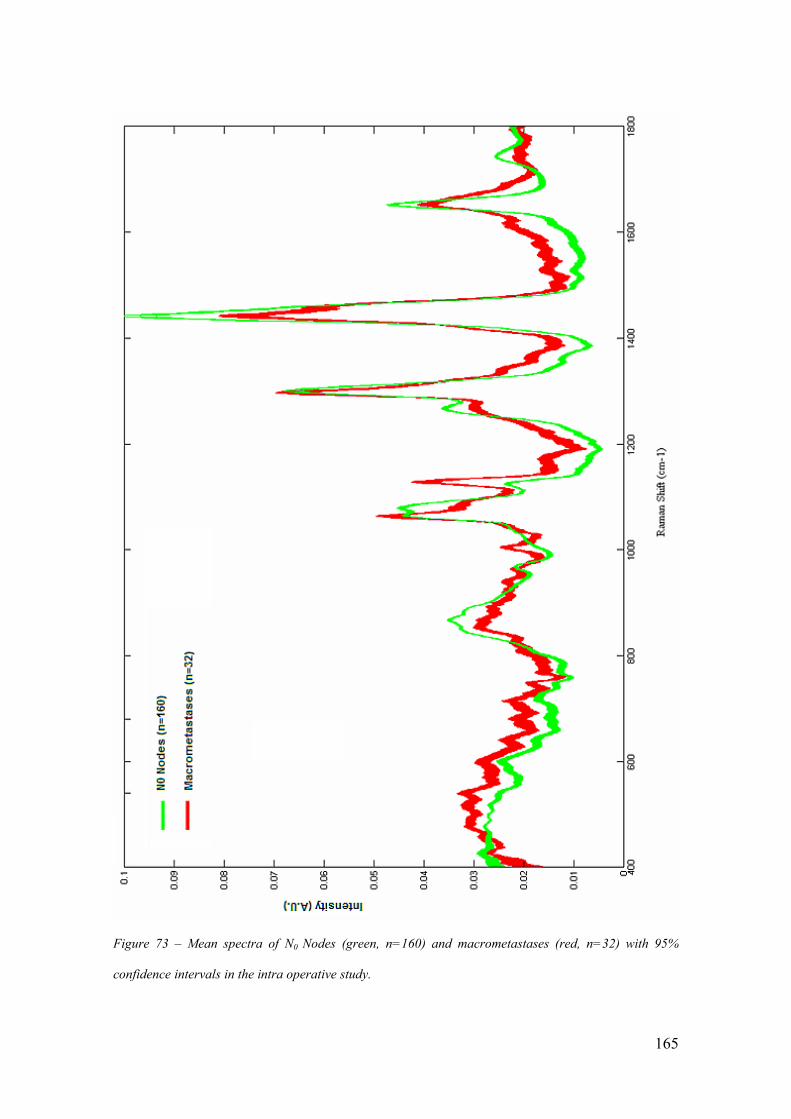
165
Figure 73 – Mean spectra of N0 Nodes (green, n=160) and macrometastases (red, n=32) with 95%
confidence intervals in the intra operative study.

166
Figure 74 – Plot of spectral subtraction to demonstrate key areas of spectral differences between N0
Nodes (n=160) and macrometastases positive nodes (n=32) in the intraoperative study . Where the plot is
green the peaks are more prominent in the N0 spectra and where the plot is red the peaks are more
prominent in macrometastases spectra. Labelled peaks are discussed further in table 19.

167
Examination of the plots of the subtracted differences enabled us to identify the
wavenumbers associated with each of the positive and negative peaks. Peak labelling
and assignation was performed using Matlab® programmes and compiled tables of peak
assignments held within the department (Kendall 2002). In this way a total of 34 peaks
that appeared significant were labelled and their biochemical association recorded
(Table 14).
Peak
Label in
Fig. 79
Peak
Position
(cm-1
)
Biochemical
assignation
Mean peak
intensity N0 nodes
(SD and SEM)
Mean peak intensity
macrometastases
(SD and SEM)
t
Value
p
Value
a 510 Disulphide 0.026
(0.002, 0.00016)
0.031
(0.0021, 0.0007)
12.8 p<0.0001
b 525 Disulphide 0.026
(0.003, 0.00026)
0.030
(0.0032,0.0006)
6.3 <0.0001
c 540 Disulphide 0.025
(0.005, 0.0004)
0.032
(0.0039,0.0007)
7.5 p<0.0001
d 571 Trytophan 0.021
(0.006, 0.0004)
0.027
(0.0038, 0.0007)
5.7 p<0.0001
e 642 Tyrosine 0.018
(0.008, 0.0006)
0.023
(0.0042, 0.0007)
3.5 p=0.0007
f 681 Guanine 0.015
(0.008, 0.0006)
0.021
(0.005, 0.0009)
4.1 p<0.0001
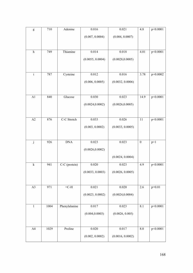
168
g 710 Adenine 0.016
(0.007, 0.0004)
0.021
(0.004, 0.0007)
4.8 p<0.0001
h 749 Thiamine 0.014
(0.0055, 0.0004)
0.018
(0.0028,0.0005)
4.01 p<0.0001
i 787 Cysteine 0.012
(0.006, 0.0005)
0.016
(0.0032, 0.0006)
3.78 p=0.0002
A1 840 Glucose 0.030
(0.0024,0.0002)
0.023
(0.0026,0.0005)
14.9 p<0.0001
A2 876 C-C Stretch 0.033
(0.003, 0.0002)
0.026
(0.0033, 0.0005)
11 p<0.0001
j 926 DNA 0.023
(0.0026,0.0002)
0.023
(0.0024, 0.0004)
0 p=1
k 941 C-C (protein) 0.020
(0.0033, 0.0003)
0.023
(0.0026, 0.0005)
4.9 p<0.0001
A3 971 =C-H 0.021
(0.0023, 0.0002)
0.020
(0.0024,0.0004)
2.6 p=0.01
l 1004 Phenylalanine 0.017
(0.004,0.0003)
0.023
(0.0026, 0.005)
8.1 p<0.0001
A4 1029 Proline 0.020
(0.002, 0.0002)
0.017
(0.0016, 0.0002)
8.0 p<0.0001

169
m 1062 ?DNA ?Lipid 0.042
(0.004,0.0003)
0.046
(0.0053,0.0009)
4.8 p<0.0001
A5 1079 C-C Stretch
Lipid
0.044
(0.007, 0.0005)
0.033
(0.0054, 0.0009)
8.4 p<0.0001
n 1130 C-N protein 0.021
(0.007, 0.0005)
0.038
(0.009, 0.0002)
12.1 p<0.0001
o 1172 C-O stretch/
Tyrosine
0.007
(0.005,0.0004)
0.016
(0.004, 0.0007)
9.5 p<0.0001
p 1205-
1213
Thiamine/
Tyrosine/
Phenylalanine
0.006
(0.005,0.0004)
0.012
(0.004,0.0007)
6.4 p<0.0001
Q 1231 Amide III 0.012
(0.005, 0.0004)
0.018
(0.004, 0.0007)
6.4 p<0.0001
A6 1263 Lipid (=C-H) 0.034
(0.004, 0.0003)
0.029
(0.003, 0.0005)
6.7 p<0.0001
R 1293 Amide III 0.055
(0.007, 0.0005)
0.059
(0.009, 0.0002)
2.8 p<0.0001
A7 1306 Lipids 0.060
(0.012, 0.0009)
0.049
(0.007, 0.001)
5.0 p<0.0001
S 1348 Nucleic Acid/
Tyrptophan/
Adenine
0.014
(0.005, 0.0004)
0.022
(0.004, 0.0007)
8.5 p<0.0001

170
T 1376-
1397
Thymine/
adenine/
guanine
0.010
(0.005,0.0004)
0.017
(0.003, 0.0005)
7.6 p<0.0001
A8 1440 Lipids 0.095
(0.022, 0.0012)
0.07
(0.013, 0.002)
6.2 p<0.0001
U 1479 Purine Bases 0.019
(0.002, 0.00016)
0.023
(0.002, 0.0004)
10.3 p<0.0001
V 1536 Tryptophan 0.009
(0.006, 0.0005)
0.015
(0.003, 0.0005)
5.5 p<0.0001
W 1609 Tyrosine 0.013
(0.006, 0.0005)
0.022
(0.004, 0.0007)
8.2 p<0.0001
A9 1652 Lipid 0.046
(0.007, 0.0005)
0.039
(0.005, 0.0009)
6.2 p<0.0001
X 1673 Amide III 0.021
(0.006, 0.0005)
0.029
(0.004, 0.0007)
7.22 p<0.0001
A10 1746 C=O stretch
lipid
0.025
(0.002, 0.0002)
0.020
(0.003, 0.0005)
11.7 p<0.0001
Table 19- Peak assignments of the key spectral differences highlighted by spectral subtraction and
labelled in Figure 74 (Kendall 2002). The mean intensity for each of these peaks in N0 nodes and
macrometastases is also given, along with their standard deviation and standard error of the mean. The
results of an unpaired t-test are also shown (both the t value and the p value) (SD=standard deviation,
SEM= standard error of the mean).

171
To add a degree of robustness to this process and to ensure that any significant peak
differences had not been missed statistical analysis of the mean intensity of each
wavenumber in the two groups was performed. An unpaired t-test was performed and
the degree of freedom for the analysis was calculated. The unpaired t-test was chosen
as it is a statistical test that compares the mean of one variable between two groups.
A null hypothesis was defined which stated that there was no difference in the mean
peak intensity between the two groups. The t value was compared to standard tables of
significance to determine whether the difference between the means was unlikely to
have occurred by chance alone. The level of statistical significance was set at 99%, thus
if the t value was greater than the published value for this significance level with 190
degrees of freedom, 2.6, then the null hypothesis could be rejected. All but 2 of the
previously identified peaks had t values which allowed us to reject the null hypothesis.
The two peaks that did not achieve this were those labelled A3 and J at 971 and 926cm-
1 respectively. These were then excluded from further evaluation.
The t values for each wavenumber were examined and used to identify further
significant differences between the two groups. It was evident that three further
wavenumbers, that had not been initially selected, recorded highly significant t values.
These were found;
below peak a at 488cm-1
(N0 mean = 0.027 (standard deviation (SD) = 0.001,
standard error of the mean (SEM) 0.0001) v. macrometastases mean 0.031 (SD
= 0.001, SEM = 0.0005)).

172
above peak a2 at 889cm-1
(N0 mean = 0.031 (SD = 0.002, SEM = 0.0002 v.
macrometastases mean 0.026 (SD = 0.003, SEM = 0.0005)).
above peak t at 1419cm-1
(N0 mean = 0.025 (SD = 0.002, SEM = 0.0002) v.
macrometastases mean 0.031 (SD = 0.003, SEM = 0.0005)).
The t values for these peaks were 13.7, 11.8 and 14.2 respectively. Potential peak
assignments of glycogen, CH2 rock and adenine/guanine were made based on available
tables. The t values for the 32 peaks identified initially and the 3 further wavenumbers
identified confirm that there are statistically significant differences between the two
groups. As spectrum recorded in Raman spectroscopy is based on the molecular
composition of the tissues being assessed these spectral differences can be assigned to
molecular differences between the two groups.
Evaluation of the different peaks associated with each pathology subgroup suggests
significant differences in the biochemical composition. Analysis demonstrated that the
positive nodes had increased relative levels of protein and nucleotides in comparison to
the true negative nodes. This is supported by the peaks associated with disulphide and
C-N bonds (510, 525, 540 and 1130 cm-1
) amide III (1293 and 1673 cm-1
) as well as
those associated with amino acids such as phenylalanine (1004 cm-1
), tryptophan (1348
and 1546 cm-1
) tyrosine (642, 1172, 1609 cm-1
) as well as the region 1205-1213 cm-1
.
Peaks associated with adenine (710 and 1348 cm-1
), cystine (787 cm-1
), thiamine (749
cm-1
) and guanine (681 cm-1
) and in the region 1376-1397 cm-1
all support the increased
intensity of DNA within metastatic nodes. Within the negative nodes peaks at 876,
1079, 1263, 1306, 1440, 1652, and 1746 cm-1
are associated with lipids and support the

173
relative increased levels of lipids within negative nodes. The peak at 840 and 894 cm-1
suggest that there may also be increased levels of glycogen and glucose in the normal
nodes. These findings are both consistent with previous studies of lymph nodes using
Raman spectroscopy and with the histological changes that occur during cancer cell
metastases. In areas where metastatic cells predominant their large nuclei account for
the increased levels of DNA and the decreased levels of lipid associated with normality.
The increased protein levels correlate with an up regulation of the immune response due
to the presence of foreign cells and the decrease in energy stores maybe accounted for
by the energy requirements of rapidly replicating cancer cells that have lost their normal
cell regulatory mechanisms.
These initial results confirmed that there were significant differences between the two
pathological groups. Further, using peak assignment, it was demonstrated that these
differences appeared to represent biochemical changes within the node. These results
were consistent with previous work, presented in Chapter 2, which has shown decreased
lipid and increased protein and DNA spectral contributions in malignant tissue.
4.2.1. Dataset 1- Diagnostic Tool.
4.2.1.1. Molecular Differences.
The next stage in the analysis of the data was to determine if the results could be used to
differentiate between the positive (macrometastases) and the N0 nodes. An initial model
was based on the relative intensities of the lipid, protein and DNA peaks that had been

174
highlighted above. The combined intensity of the 9 peaks attributed to lipids, the 15
peaks related to proteins and the 10 peaks attributed to DNA were combined for each
node to give a lipid, protein and DNA score. Separation of the two groups was then
attempted based on each of these three values and finally the combined value of the
three intensities. As it was expected that the lipid value would be higher in the negative
nodes and that the protein and DNA value would be higher in the positive nodes an
overall score was calculated based on the formula given below. The lipid score was
subtracted from 0.5 as no node achieved a value of greater than 0.45.
Overall Score= (Protein score + DNA score) + (0.5-lipid score)
Plots of each of these composition scores highlighted the differences between the
macrometastases and N0 samples (Figure75-79). Although these compositional scores
demonstrated statistically significant differences between the two pathology sub-groups,
using an unpaired t-test (Table 20) (Figure 80) they were not sufficient to separate them
with a sensitivity and specificity sufficient for clinical use.
It is interesting to note the negative nodes appear to separate into two further subgroups
based on the protein score. It is postulated that this may reflect either a greater immune
response in nodes earlier in the nodal chain or that it may represent a response to recent
breast biopsies or due to isolated histopathologically undetected metastatic cells.

175
0.25 0.3 0.35 0.4 0.45 0.50
50
100
150
200
250
Lipid Component
Spe
ctra
No.
Figure 75 – Histogram demonstrating the combined intensity of all lipid related peaks for each spectra in
dataset 1 (green = N0 negative nodes, red= macrometastases positive nodes).
0.2 0.25 0.3 0.35 0.4 0.45 0.50
20
40
60
80
100
120
140
Spe
ctra
No.
Protein Contribution
Figure 76 – Histogram demonstrating the combined intensity of all protein related peaks for each spectra
in dataset 1 (green = N0 negative nodes, red= macrometastases positive nodes).

176
0.15 0.2 0.25 0.30
20
40
60
80
100
120
140S
pect
ra N
o.
DNA contribution
Figure 77 – Histogram demonstrated the combined intensity of all DNA related peaks for each spectra in
dataset 1 (green = N0 negative nodes, red= macrometastases positive nodes).
0.4 0.5 0.6 0.7 0.8 0.9 10
50
100
150
Spe
ctra
No
Overall Score
Figure 78 – Histogram demonstrating the overall score for positive and negative nodes for each spectra
in dataset 1(green = N0 negative nodes, red= macrometastases positive nodes).

177
0.25
0.3
0.35
0.4
0.45
0.5
0.20.25
0.30.35
0.40.45
0.5
0.15
0.2
0.25
0.3
Protein Contributionlipid Contribution
DN
A C
ontr
ibution
Figure 79 –3D plot demonstrating the ability of the three scores (lipid, protein and DNA contribution) to
separate macrometastases positive nodes (red) from N0 negative nodes(green) in dataset1.
Mean
Lipid Score
(SD, SEM)
Mean
Protein Score
(SD, SEM)
Mean
DNA Score
(SD, SEM)
Mean
Combined Score
(SD, SEM)
Macrometastases
(n=32)
0.32
(0.03, 0.005)
0.40
(0.04,0.007)
0.24
(0.02, 0.004)
0.82
(0.06, 0.01)
N0 Negative
(n=160)
0.40
(0.05, 0.004)
0.30
(0.06,0.005)
0.19
(0.04, 0.003)
0.59
(0.04, 0.003)
Unpaired t-test p<0.0001
t=8.29
p<0.001
t=9.02
p<0.001
t=6.9
P<0.001
t=27
Table 20: The total intensities of peaks attributable to lipid, protein and DNA in the macrometastases and
N0 groups. Results of an unpaired t-test confirm the statistical significance of these differences.

178
Figure 80 – Box and Whisker plots demonstrating the mean and 95% confidence intervals for the
contributions of lipid, protein and DNA peaks as well as the overall molecular score for macrometastases
(positive, green) v N0 (negative, green) nodes (see also table 14a).

179
The combined compositional score was then used to assess whether it could be used to
discriminate between positive and negative nodes. Analysis of the data suggested that
the “score” which best discriminated between the two groups was 0.75. If a node had a
combined score of greater than 0.75 it was defined as positive and if the combined score
was less than 0.75 it was defined as negative. Using this score a sensitivity of 81%
(27/32) and a specificity of 84% (128/160) was achieved. Whilst the sensitivity is at
least comparable to current intraoperative techniques the specificity is significantly
worse. As has been discussed this is clinically of most significance to avoid ultimately
unnecessary axillary dissections and adjuvant chemotherapy. To investigate how the
specificity could be improved the calculation was repeated with separation scores of 0.7
to 0.9. As the score was raised the specificity did indeed improve but at the expense of
the sensitivity (Table 21).
Combined Score Diagnostic Cut
Off Point
(if > cut off = positive)
Sensitivity
(%)
Specificity
(%)
0.7
84
80
0.75
81
84
0.8
72
86
0.85
56
91
Table 21- Change in sensitivity and specificity at differentiating between macrometastases nodes and N0
nodes using a combined biochemical score ((protein + DNA contribution) + (0.5 – lipid contribution)) as
the diagnostic cut off point is altered.

180
Whilst these results are encouraging it was felt that they would not acceptable for a
diagnostic test within this clinical scenario. Therefore further methods of data analysis
were required to develop the technique as a diagnostic tool.
4.2.1.2. Principal Component Analysis fed Linear Discriminant
Analysis (PCA fed LDA)
Due to the complexity of the data contained within a spectrum many authors have used
chemometric recognition techniques to help interpret the information. A widely used
technique is linear discriminant analysis (LDA) fed by principal component analysis
(PCA). Using PCA allows one to simplify the data into fewer variables whilst retaining
the overall spectral information. Each dataset is split into a number of components
(loads) which contribute to each of the spectrum within the dataset. The contribution of
each component is different for each spectrum and is defined by the principal
component score. Each original spectrum has a different score for each load. The scores
for each principal component (PCs) can then be used to simulate a linear boundary
between the classes in the model (Sattlecker et al. 2010).
Initial data analysis used all spectra that had been collected from the nodes in the two
groups. Thus a total of 1325 negative spectra and 290 positive spectra were included.
When PCA fed LDA was performed a specificity of 99% and sensitivity of 95% was
achieved. However it was felt that in a clinical scenario all spectra acquired from a
single sample would be combined to provide a single output for each node. Therefore
the mean of the spectra collected from each sample was subsequently assessed.

181
-0.08 -0.06 -0.04 -0.02 0 0.02 0.040
20
40
60
80
100
120
140
160N
um
ber
of
Spectr
a
PCA fed LDA score
Figure 81 – PCA fed LDA scores for spectra from macrometastases positive samples (red) and N0
negative samples (green) in dataset 1.
After mean centring the processed spectral data, principal component analysis was
performed to generate 25 PC loads and scores. An unpaired t-test was performed to
assess the statistical significance of the differences between the mean of the 25 scores
for both positive and negative nodes. For each of the principal components the null
hypothesis was that there was no difference between the mean score in the two groups.
With 188 degrees of freedom the null hypothesis could be rejected at the 99%
confidence level if the t score generated was greater than 2.6. Only 4 PCs achieved this
level of significance, PC 1, 2, 11 and 12 (Figure 82, 83).
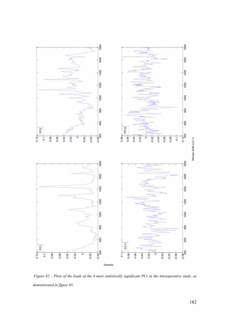
182
Figure 82 – Plots of the loads of the 4 most statistically significant PCs in the intraoperative study, as
demonstrated in figure 83.
400
600
800
1000
1200
1400
1600
1800
-0.0
4
-0.0
20
0.0
2
0.0
4
0.0
6
0.0
8
0.1
0.1
2
400
600
800
1000
1200
1400
1600
1800
-0.0
6
-0.0
4
-0.0
20
0.0
2
0.0
4
0.0
6
0.0
8
0.1
0.1
2
400
600
800
1000
1200
1400
1600
1800
-0.0
8
-0.0
6
-0.0
4
-0.0
20
0.0
2
0.0
4
0.0
6
0.0
8
0.1
400
600
800
1000
1200
1400
1600
1800
-0.1
2
-0.1
-0.0
8
-0.0
6
-0.0
4
-0.0
20
0.0
2
0.0
4
0.0
6
0.0
8
Ram
an S
hift
(cm
-1)
Intensity
PC
12
PC
11
PC
2P
C1

183
0 5 10 15 20 250
5
10
15
PC Number
T S
tatis
tic
99% statistical level
Figure 83 – t score from an unpaired t-test to assess the statistical significance of differences in the mean
value of the scores for the first 25 PCs between macrometastases and N0 node (n=32 and n= 160
respectively) .The horizontal line represents the 99% statistical level.
Closer examination of PC1 revealed peaks at positions identical or very similar to those
previously identified as representative of negative nodes (Figure 84). Examination of
PC 2 revealed that there were 20 of the peaks previously identified as positive evident in
the plot (Figure 85). It was postulated that PC1, resembling lipids, represented negative
nodes and that PC2, representing a combination of protein and DNA, was representative
of positive nodes. This is supported by the finding that the mean score for PC1 amongst
the positive nodes is -0.155 whereas that of the negative nodes is 0.03. Similarly for
PC2 the mean score for the negative nodes is -0.17 and for the positive nodes it is 0.085.

184
Figure 84- Plot of PC1 from principal component analysis of the dataset No and macrometastases nodes
with key peaks marked for clarity.
400
600
800
1000
1200
1400
1600
1800
-0.0
4
-0.0
20
0.0
2
0.0
4
0.0
6
0.0
8
0.1
0.1
2
Ram
an S
hift
cm
-1
Intensity
840
875
1079
1269
1303
1439
1651
1744
975
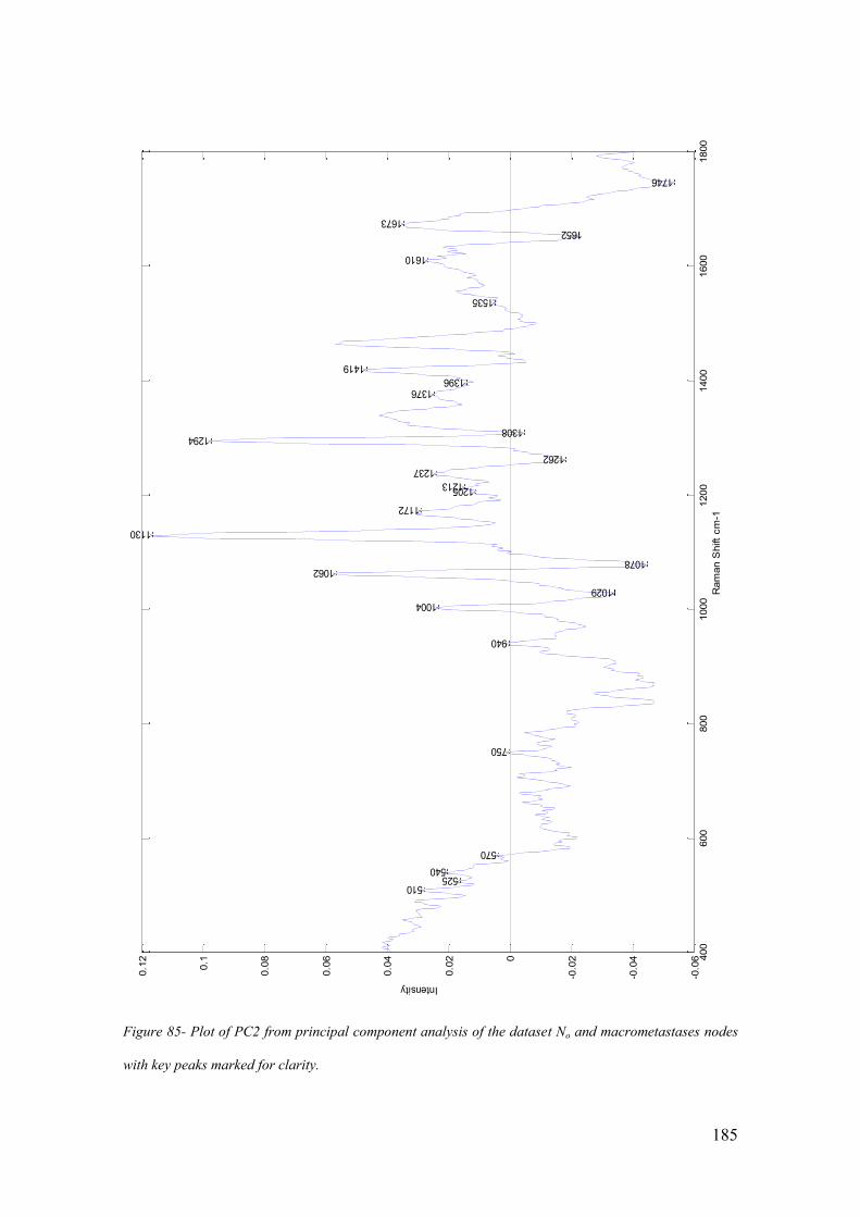
185
Figure 85- Plot of PC2 from principal component analysis of the dataset No and macrometastases nodes
with key peaks marked for clarity.
400
600
800
1000
1200
1400
1600
1800
-0.0
6
-0.0
4
-0.0
20
0.0
2
0.0
4
0.0
6
0.0
8
0.1
0.1
2
1376
Ram
an S
hift
cm
-1
Intensity
510525
540
570
750
940
1004
1062
1130
1172
12051213
1237
1294
1396
1419
1535
1610
1673
1029
1078
1262
1308
1652
1746
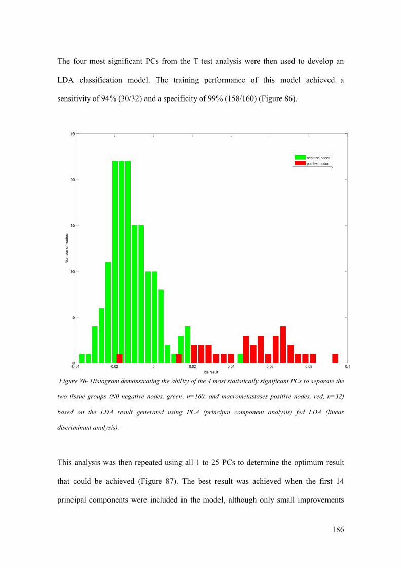
186
The four most significant PCs from the T test analysis were then used to develop an
LDA classification model. The training performance of this model achieved a
sensitivity of 94% (30/32) and a specificity of 99% (158/160) (Figure 86).
-0.04 -0.02 0 0.02 0.04 0.06 0.08 0.10
5
10
15
20
25
Num
ber
of
nodes
lda result
negative nodes
positive nodes
Figure 86- Histogram demonstrating the ability of the 4 most statistically significant PCs to separate the
two tissue groups (N0 negative nodes, green, n=160, and macrometastases positive nodes, red, n=32)
based on the LDA result generated using PCA (principal component analysis) fed LDA (linear
discriminant analysis).
This analysis was then repeated using all 1 to 25 PCs to determine the optimum result
that could be achieved (Figure 87). The best result was achieved when the first 14
principal components were included in the model, although only small improvements

187
are made beyond the first two PCs. Using PCs 1 to 14 to train the LDA model a
sensitivity of 96.9% (31/32) and a specificity of 99.4% (159/160) was achieved in the
training model.
0 5 10 15 20 250
10
20
30
40
50
60
70
80
90
100
Number of Principal Components
perc
enta
ge
Sensitivity
Specificity
Figure 87– Improvement in the sensitivity(red) and specificity (blue) with increasing numbers of PC in
dataset 1 (N0 negative and Macrometastases positive nodes) .
The robustness of this data was further tested by using leave one node out cross
validation. In this test the data from one sample is left out and the data from the
remaining samples is then used to build a training set. This training set is split according
to known pathology results and is used to predict the group membership, in this case
positive or negative node, of the sample that had been left out. The leave one node out
testing achieved a specificity of 99.4% (159/160) and a sensitivity of 93.8% (30/32)

188
when using all 25 PCS. When using only 14 PCs which we have previously shown
achieved the best training set result using LDA a specificity of 98.8%(158/160) and a
sensitivity of 90.6% (29/32) was achieved (Fig 88).
0 5 10 15 20 250
0.1
0.2
0.3
0.4
0.5
0.6
0.7
0.8
0.9
1
Specificity
Sensitivity
Figure 88- Improvement in the cross validation based sensitivity (red) and specificity (green) with
increasing numbers of PC in dataset 1 (N0 negative and Macrometastases positive nodes) .
This data was then used to assess the clinical impact it would have had on the patients
involved in the study had it been used to guide clinical decisions. This dataset included
nodes samples from 48 patients undergoing a SLNB. On subsequent histopathological
testing Of the 57 sentinel lymph node biopsies performed 40 a negative axilla and 8 had
evidence of macrometastases. If the results of the leave one node out cross validation

189
testing had been used, 38 out of 40 (95%) patients with a negative axilla would have
been correctly identified. 6 out of 8 (75%) patients with an axilla containing
macrometastases would have been correctly identified and would have benefited from
an immediate axillary clearance. Thus 2 patients would have suffered from a false
positive result and had an unnecessary axillary clearance. The two patients with false
negatives would have been identified following post operative gold standard node
assessment and recommended a delayed axillary clearance. These results are
comparable to both other Raman spectroscopic studies (outlined in Chapter 2) and the
current techniques used in the intra-operative assessment of axillary lymph nodes in
breast cancer. However it needs to be remembered that these results are for the
comparison of the two groups, macrometastases and normal nodes from N0 patients
which would be expected to demonstrate the most significant pathological differences.
4.3. Results - Dataset 2: Macrometastases v all Negative nodes.
In the second dataset a larger group of negative nodes were assessed. This included both
the negative nodes from N0 patients (n=160) and the non-N0 group (n=116). As stated
previously these nodes are those that were histopathologically negative but that came
from patients with other positive nodes. Mean spectra of the two groups were plotted
and the intensity of the same 34 peaks, that had previously been used to examine the
differences in the protein, DNA and lipid spectral contributions were calculated (Figure
89). These, along with the combined score were used to compare both between the
positive and negative groups, as well as the two negative groups.

190
The results revealed that there were slightly higher levels of DNA and protein and
slightly lower levels of lipid within the non-N0 negative group in comparison to the N0
negative group (Figure 90) (Table 22). An unpaired t-test revealed statistically
significant differences between the Non-N0 nodes and both the N0 and macrometastases
nodes (Table 23).
Mean Lipid Score
(SD, SEM)
Mean Protein
Score
(SD, SEM)
Mean DNA Score
(SD, SEM)
Mean Combined
Score
(SD, SEM)
Non N0 negative
nodes (n=116)
0.38
(0.05, 0.004)
0.32
(0.07,0.007)
0.20
(0.04, 0.004)
0.63
(0.03, 0.003)
Table 22: The intensities of peaks attributable to lipid, protein, DNA and a combined score in the non N0
negative nodes. For comparison to No nodes and macrometastases see table 20 (SD=standard deviation
and SEM= standard error of the mean).
Lipid
Score
Protein
Score
DNA
Score
Combined
Score
N0 v. Non- N0 negative nodes
p=0.009
(t=2.63)
p=0.0073
(t=2.70)
p=0.01
(t=2.60)
p<0.001
(t=9)
Macrometastases v. Non- N0
negative nodes
p<0.001
(t=8.29)
p<0.001
(t=9.02)
p<0.001
(t=6.9)
p<0.001
(t=24)
Table 23: Results of unpaired t-tests comparing the mean lipid, protein, DNA contribution and a
combined score for N0, non-N0 negative and macrometastases nodes (n=160,116 and 32 respectively).
See also tables 20 and 22 for mean, standard deviation and standard error of the mean for each group.
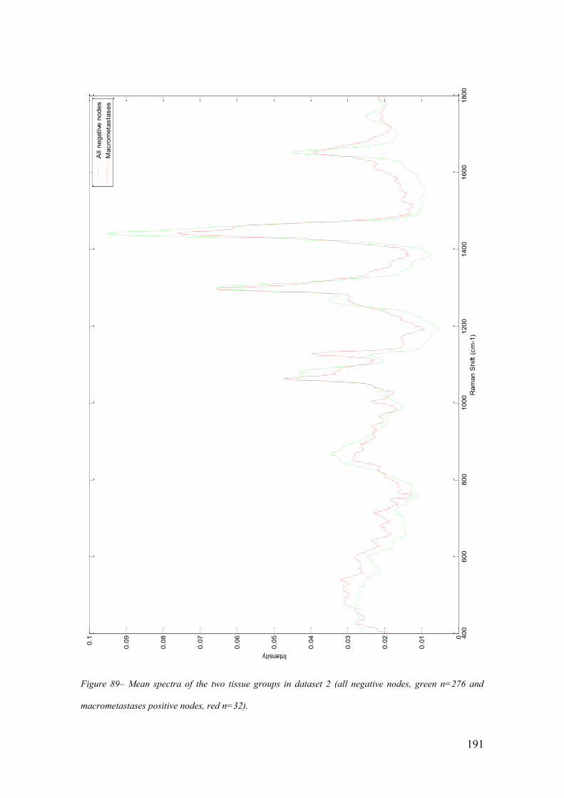
191
400
600
800
1000
1200
1400
1600
1800
0
0.0
1
0.0
2
0.0
3
0.0
4
0.0
5
0.0
6
0.0
7
0.0
8
0.0
9
0.1
Intensity
Ram
an S
hift
(cm
-1)
All n
egative
nodes
Macro
meta
sta
ses
Figure 89– Mean spectra of the two tissue groups in dataset 2 (all negative nodes, green n=276 and
macrometastases positive nodes, red n=32).

192
Figure 90- Mean intensity scores (with 95% confidence intervals) for peaks related to Protein, DNA and
lipid and a combined score in dataset 2. (N0 (green,) non-N0 negative (orange) and macrometastases
(red) nodes (n=160,116 and 32 respectively)).

193
If a combined score of 0.7 was used as a diagnostic cut of a sensitivity of 84% and a
specificity of 76% was achieved. As previously demonstrated in the first model if the
score required to differentiate between the two groups rose then the sensitivity fell and
the specificity rose (Table 24).
Combined Score Diagnostic Cut
Off Point
Sensitivity Specificity
0.7 84 76
0.75 81 80
0.8 72 84
0.85 56 89
Table 24- Change in sensitivity and specificity as the diagnostic cut off point is altered in dataset 2.
As outlined earlier in this chapter principal component fed linear discriminant analysis
was then used to differentiate between the negative and macrometastases groups. The
best sensitivity achieved was 91% (29/32) and the best specificity achieved was 98%
(270/276) when using 25 PCs. Leave one node out cross validation testing was
performed and a specificity of 96% (265/276) and a sensitivity of 84% (27/32) were
achieved. Whilst still very acceptable this result is poorer than that achieved in the true
negative v macrometastases model.
This result prompted questions as to why this was the case? It could be postulated that
there are changes in the non-N0 negative group that are due to the immune response to
metastases in another node, as detailed in Chapter 1. This is supported by the results of

194
the individual component analysis that demonstrated that the differences in the protein
score were the most statistically significant between the N0 negative nodes and the non-
N0 negative groups. The mechanism behind this difference may be explained by
immune mediators produced in response to metastatic deposits in other nodes being
filtered through nodes higher in the chain. These differences would not render the node
“positive” pathologically but could alter the spectral features of the sample sufficiently
to influence the classification model. This is an important finding to be aware of in the
future particularly if models are created based on this data. Misclassification of these
non-N0 nodes is in itself not likely to be clinically important as other nodes would
already have seen the patient classified as having a positive axilla. Their role however in
altering the model classification could render positive nodes negative as it has done in
this dataset and increase the false-negatives.
4.4. Results - Dataset 3: All Positive nodes (Macro+Micro+ITCs) v Negative
Nodes.
The final dataset included the macrometastases (n=32), the micrometastases (n=8), the
isolated tumour cells (n=10) and all the negative nodes (n=276). As the micrometastases
and ITC group sizes were so small these were combined into one group term “non-
macrometastases positive nodes” (n=18).As discussed previously the protein, lipid and
DNA scores for each sample were calculated (Table 25). The differences between the
macrometastases and the “non-macrometastases” positive nodes were statistically
significant for lipid, protein and DNA. Although none of the changes were statistically
significant for “non macrometastases” positive nodes versus N0 negative nodes and non
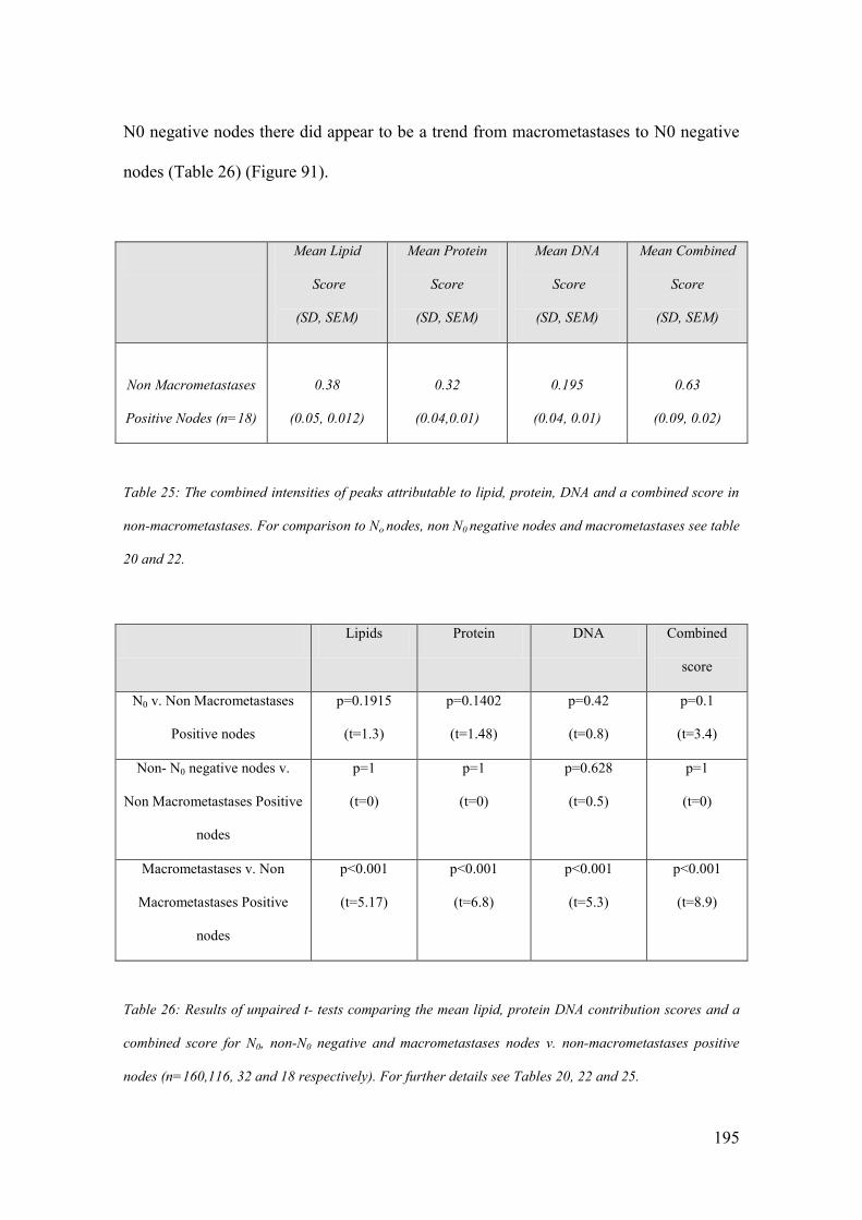
195
N0 negative nodes there did appear to be a trend from macrometastases to N0 negative
nodes (Table 26) (Figure 91).
Mean Lipid
Score
(SD, SEM)
Mean Protein
Score
(SD, SEM)
Mean DNA
Score
(SD, SEM)
Mean Combined
Score
(SD, SEM)
Non Macrometastases
Positive Nodes (n=18)
0.38
(0.05, 0.012)
0.32
(0.04,0.01)
0.195
(0.04, 0.01)
0.63
(0.09, 0.02)
Table 25: The combined intensities of peaks attributable to lipid, protein, DNA and a combined score in
non-macrometastases. For comparison to No nodes, non N0 negative nodes and macrometastases see table
20 and 22.
Lipids Protein DNA Combined
score
N0 v. Non Macrometastases
Positive nodes
p=0.1915
(t=1.3)
p=0.1402
(t=1.48)
p=0.42
(t=0.8)
p=0.1
(t=3.4)
Non- N0 negative nodes v.
Non Macrometastases Positive
nodes
p=1
(t=0)
p=1
(t=0)
p=0.628
(t=0.5)
p=1
(t=0)
Macrometastases v. Non
Macrometastases Positive
nodes
p<0.001
(t=5.17)
p<0.001
(t=6.8)
p<0.001
(t=5.3)
p<0.001
(t=8.9)
Table 26: Results of unpaired t- tests comparing the mean lipid, protein DNA contribution scores and a
combined score for N0, non-N0 negative and macrometastases nodes v. non-macrometastases positive
nodes (n=160,116, 32 and 18 respectively). For further details see Tables 20, 22 and 25.

196
Figure 91- Mean intensity scores (with 95% confidence intervals) for peaks related to Protein, DNA and
lipid and a combined score in N0 (green,) non-N0 negative(orange), non-macrometastases positive nodes
(light red) and macrometastases(dark red) nodes (n=160,116,18 and 32 respectively)

197
The width of the standard error bars for the non macrometastases positive nodes is
partly explained by the small group size but may also be explained by the presence of
what appear to be two distinct subsets within the data (Figure 98). In one subset there
are high levels of lipid with low levels of protein and DNA (resembling negative nodes)
and in the other there are low levels of lipid with high levels of protein and DNA
(resembling the macrometastases nodes). These two subsets are not related to a
comparison between the ITCs vs. Micrometastases. Chemometric analysis revealed that
only 50% (4/8) of the micrometastases and 40% (4/10) of the ITCs were correctly
categorised. The small group size made further evaluation of this finding difficult but it
could be suggested that one reason for the difference was that an insufficient volume of
the node is being sampled to detect the small areas of change associated with either
micrometastases or isolated tumour cells in those samples that appeared similar to the
negative nodes. It is not altogether surprising that those eight samples that were
correctly categorised were the eight that had features most closely resembling the
positive nodes and thus would be examples of where the nodal change was identified
from the volume of tissue analysed (Figure 92).
These results demonstrate the difficulties that may be experienced detecting
micrometastases and isolated tumour cells using this technique. As was discussed in
Chapter 1 it is likely that a decision to proceed to an ALND would not be clear cut and
that MDT discussion would be required prior to proceeding to an ALND.

198
0.2
0.25
0.3
0.35
0.4
0.45
0.3
0.32
0.34
0.36
0.38
0.4
0.42
0.16
0.18
0.2
0.22
0.24
0.26
0.28
Protein
Lipid
DN
A
Figure 92- 3d plot of the lipid, protein and DNA contributions in micrometastases and ITC
demonstrating two clear groups, one with high DNA and protein contributions and low lipid
contributions (consistent with a positive node) and one group with lower DNA and protein contributions
and high lipid contributions (consistent with a negative node). This supports the suggestion that in the
micrometastases and isolated tumour cell samples because of the small volume of disease this was not
being ”seen” by the Raman technique in all of the nodes investigated.

199
4.5. Measurements from the inner cut surface versus those from the outer
surface.
Discussion within the group at the outset of this study questioned whether spectra
needed to be obtained from the cut inner surface of lymph nodes, as had previously been
performed, or whether spectra could be collected from the outer surface of the node
without altering the sensitivity and specificity of the test. Looking forward this would
mean that lymph node analysis might be able to be performed with the node still in situ
and negate the need to excise the lymph node if it were negative. Various groups
throughout the world are beginning to develop either minimally invasive lymph node
sampling or in a few centres laparoscopic sampling techniques (Lim and Lam 2005). If
Raman spectroscopy could differentiate between positive and negative nodes based on
spectra obtained from the outer surface of the node this technique would be further
enhanced and the invasiveness of the procedure further reduced. Further, analysis of the
results, as discussed above, suggested that further volume sampling may help improve
the detection of micrometastases and isolated tumour cells.
4.5.1. Inner vs. Outer Experiment - Methods.
282 of the samples collected during the study described at the start of Chapter 4 were
assessed both from the inner cut surface and also from the outer surface. At the time of
analysis 5 spectra were obtained from the inner cut surface and then the node was
simply turned 180° and further spectra were acquired. Spectral acquisition and tissue
handling was as described at the start of Chapter 4. Data analysis was performed using
200
Matlab® software. Statistical analysis was performed using a paired t-test to compare
the mean intensity of each wavenumber in the two datasets. The null hypothesis was
that there was no difference between the two groups at each wavenumber. The null
hypothesis was rejected if the t value was greater than 2.33 (the critical value for a test
with >500 degrees of freedom at the 99% level). More detailed analysis of the
biochemical differences was performed by examining the mean intensity of the peaks
attributable to lipid, protein and DNA as described earlier in this chapter. Further
analysis using PC fed LDA was then performed as has been discussed earlier in this
chapter.
4.5.2. Inner vs. Outer Experiment - Results.
Of the 282 samples which were assessed in this way. 132 were negative nodes from N0
patients, 90 were negative nodes from non-N0 patients, 31 were samples with
macrometastases, 8 were samples with micrometastases, 9 had ITCs and 12 were from
fat (thus not included in further analysis). For comparative purposes two datasets with
spectra obtained from either the inner or the outer surface of each sample was created.
Mean spectra (n=270 in both groups) from the two datasets looked very similar on
initial inspection and this was confirmed by performing a paired t-test on each of the
wavenumbers (Figure 93, 94).

201
Figure 93 – Mean spectra collected from the outer (n=270, green) and inner surface (n=270, blue) of the
lymph nodes.
400
600
800
1000
1200
1400
1600
1800
0
0.0
1
0.0
2
0.0
3
0.0
4
0.0
5
0.0
6
0.0
7
0.0
8
0.0
9
0.1
Ram
an S
hift
(cm
-1)
Intensity
inner
measure
ments
oute
r m
easure
ments

202
Figure 94 –The results of the t-test for each wavenumber to demonstrate the statistical significance of the
differences between the mean intensity of each wavenumber for spectra from the inner and outer surface
of each lymph node. Statistical significant differences were only present if the t-value was above 1.66
(95% significance level) or 2.33 (99% significance level).

203
The null hypothesis was only rejected for one wavenumber at 1321 cm-1
. Even if the
significance level is reduced to 95% the null hypothesis is rejected at only two further
wavenumbers at 469 and 1282 cm-1
. Chemometric analysis was then performed on the
data to calculate whether the two sets of data could be categorised. The differences
between the two groups were not sufficient to differentiate between the spectra obtained
from inner or outer surfaces. The overlap between the two groups was very evident
when the scores for the LDA analysis were plotted (Figure 95). These findings therefore
support the statement that there is little difference between the mean spectra acquired
from the outer and inner half of the lymph node.
-0.03 -0.02 -0.01 0 0.01 0.02 0.03 0.040
5
10
15
20
25
30
35
40
45
50
Num
ber
of
sam
ple
s
LDA score
Spectra from inner surface
Spectra from outer surface
Figure 95–PCA fed LDA scores for spectra from the inner (blue) and outer (green) surface of each node
demonstrating the difficulty separating the two datasets.

204
Whilst the results from the overall mean spectra were encouraging it was theorised that
greater differences may be seen in the nodes with metastatic disease. As previously
discussed metastatic cells that have spread to axillary lymph nodes are first found in the
subscapular sinuses before passing to the medullary sinuses from where they penetrate
the medulla, then the cortex, and eventually can result in parenchymal replacement
(Iochim and Ratech 2009). Thus although isolated metastatic cells may be found near to
the outer surface of the node large macrometastases are more likely to be found in the
centre of the node.
Thus a dataset was created that included the spectra from the macrometastases positive
nodes (that had been acquired from both the inner and the outer surface of the node) and
the spectra obtained from the inner surface of the N0 negative nodes. When the mean
spectra of the macrometastases samples acquired from the inner surface were plotted
with the mean spectra of the macrometastases samples acquired from the outer surfaces
clear differences are evident. If the mean spectra acquired from the inner surface of the
N0 negative nodes were plotted on the same graph it is clear that the mean spectra from
the outer surface of the macrometastases nodes has shifted towards the mean spectra
from the true negative nodes (Figure 96).

205
400
600
800
1000
1200
1400
1600
1800
0
0.0
1
0.0
2
0.0
3
0.0
4
0.0
5
0.0
6
0.0
7
0.0
8
0.0
9
0.1
Ram
an S
hift
cm
-1
Intensity
inner
spectr
a
oute
r spectr
a
inner
norm
al
Figure 96 – Mean spectra collected from the outer (orange dash, n=31) and inner (red, n=32) surface of
the lymph nodes with metastatic spread and the inner surface of normal nodes (green, n=160).
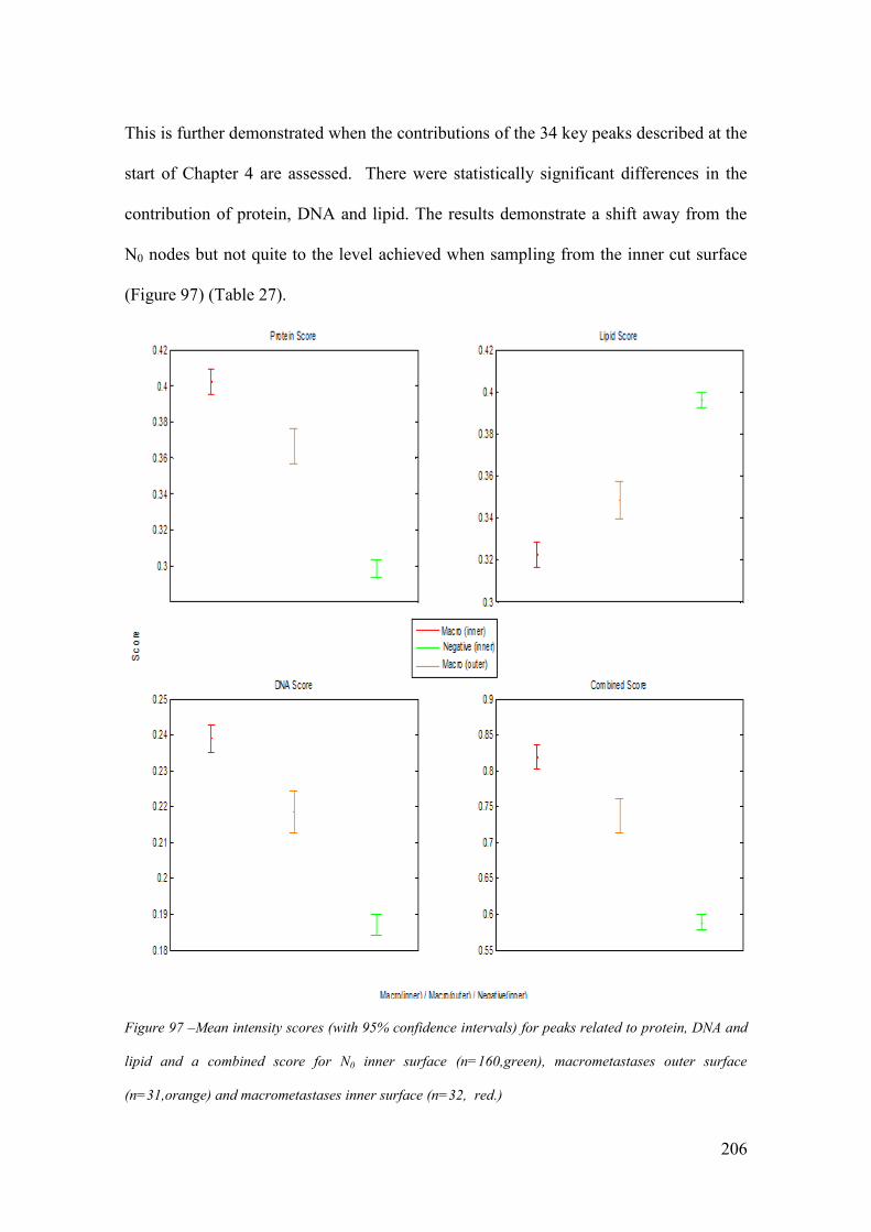
206
This is further demonstrated when the contributions of the 34 key peaks described at the
start of Chapter 4 are assessed. There were statistically significant differences in the
contribution of protein, DNA and lipid. The results demonstrate a shift away from the
N0 nodes but not quite to the level achieved when sampling from the inner cut surface
(Figure 97) (Table 27).
Figure 97 –Mean intensity scores (with 95% confidence intervals) for peaks related to protein, DNA and
lipid and a combined score for N0 inner surface (n=160,green), macrometastases outer surface
(n=31,orange) and macrometastases inner surface (n=32, red.)

207
Mean Lipid
Score
(SD, SEM)
Mean Protein
Score
(SD, SEM)
Mean DNA
Score
(SD, SEM)
Mean Combined
Score
(SD, SEM)
Macrometastases Inner
(n=32)
0.32
(0.03, 0.005)
0.40
(0.04,0.007)
0.24
(0.02, 0.004)
0.82
(0.06, 0.01)
N0 Negative
(n=160)
0.40
(0.05, 0.004)
0.30
(0.06,0.005)
0.19
(0.04, 0.003)
0.59
(0.04, 0.003)
Macrometastases Outer
(n=31)
0.35
(0.03,0.005)
0.368
(0.03, 0.005)
0.2185
(0.02,0.004)
0.73
(0.05, 0.01)
1.Unpaired t-test
Inner v. Outer
2.Unpaired t-test
N0 v. Outer
p=0.004
t=3.74
p=0.007
t=3.6
p<0.001
t=4.3
P<0.001
t=6.5
p<0.001
t=4.9
p<0.001
t=6.3
p<0.001
t=4.3
p<0.001
t=17
Table 27: The combined intensity of peaks attributable to lipid, protein and DNA in the macrometastases
(inner and outer spectral collections) and N0 (inner spectral collection) groups. Results of unpaired t-tests
confirm the statistical significance of these differences and are also shown.
This effect was further interrogated by using the data to differentiate between the
positive and negative samples. PCA fed LDA and leave one node out cross validation
was again used as discussed earlier in the chapter.

208
Using leave one node out cross validation testing the test achieved a specificity of
97.7% (129/132) and a sensitivity of 81% (25/31) at differentiating between N0 negative
nodes (spectra from the inner surface) and macrometastases samples (spectra from the
outer surface) (Table 28). This was then compared to the results of the leave one node
out cross validation testing of the samples acquired from the inner surface of the
macrometastases samples which in this dataset achieved a sensitivity of 93.6% (29/31)
and a specificity of 99.2% (131/132).
Pathology
Positive Negative
Raman Positive 25 3
Negative 6 129
Sensitivity =81% Specificity=98%
Table 28- The sensitivity and specificity table with spectra from the outer surface.
An explanation for the compositional analysis results is that there is greater contribution
to the spectra from normal areas of the node when they are acquired from the outer
surface. Therefore in the 6 false negatives it could be argued that the spectral features of
the metastases were either masked by the normal areas of the node or the probe simply
did not collect information from a deep enough volume to detect them. This will have
also affected the overall model and may explain the slightly worse specificity. The
histopathology reports for these nodes demonstrate that the 6 false negative samples
have a mean diameter of 9.33mm which is beyond the sampling depth of the probe, and
that there is no evidence of extra nodal spread in any of them. Neither of the false

209
negatives from the inner surface analysis were correctly placed by assessment of the
outer surface. This suggests that currently lymph node assessment from the outer
surface of the node is not only, not as sensitive as assessment from the inner surface, but
that it may not be complimentary to the inner surface testing either. It should however
be noted that the sensitivity remains higher than that reported for frozen section and
touch imprint cytology. It therefore appears that whilst not as good as inner surface
testing then this might be worth pursuing following the establishment of an effective
testing model if the benefits of in situ testing were clear.
The dataset was then used to examine the spectra for micrometastases and ITCs
Potentially because ITCs are found in the outer capsule of the node it is possible that
spectra acquired from the outer surface of the node would be better able to detect these
small deposits than those obtained from the inner surface. This however proved not to
be the case. Using chemometric analysis a specificity of 99% (159/160) but a sensitivity
of only 33% (3/9) was achieved when differentiating ITCs from. When differentiating
between micrometastases and N0 nodes with a specificity of 99.2% the sensitivity was
37.5% (3/8). These are broadly consistent with the results of the spectral analysis of
those collected from the inner surface. Again none of the false negatives, from analysis
of the inner surface, were correctly placed using the outer surface spectra.
Based on these results nodal analysis based on spectra obtained from the outer surface
of the node as opposed to those obtained from the inner surface of the node could not be
supported. The results are poorer both for the identification of macrometastases but also
micro metastasis and ITCs. Complimentary assessment of both the inner and outer

210
surface would have not improved the correct classification of the node as the false
negatives were present in both groups. If spectral analysis from the outer surface is to be
improved then either the benefits of in-situ testing need to be significant enough to
overcome the poorer sensitivity or probes with a greater sample depth will be required
to overcome the effects of normal tissue which surrounds the metastatic deposits.
4.6. Intraoperative Work - Conclusions
The results in this chapter for the first time demonstrate the efficacy of a portable
Raman spectroscopic device at differentiating between positive and negative nodes for
patients undergoing axillary surgery for breast cancer, in real time. They are also some
of the first results that use Raman spectroscopy at the patient “bed side” to assess tissue.
The results of dataset 1 comparing N0 negative nodes to nodes positive for
macrometastases are unsurprisingly, most promising. The best results achieved are
easily comparable, if not better, than many of the currently available techniques. The
demonstration of the molecular differences that underpin these results by both
interpretation of peak positions and evaluation of the principal components generated
using PCA adds further weight to these results. Differences in the protein, DNA and
lipid concentrations within nodal tissue are consistent with the anticipated changes that
would be expected when a colony of metastatic cells invades an axillary lymph node.
The results achieved when including the negative samples from non-N0 patients and
those with micrometastases and isolated tumour cells were less encouraging. They are
however important findings as it demonstrates that future models should be built on data

211
from samples from N0 patients and samples positive for macrometastases only.
Clinically the need to discover either micrometastases or especially ITCs is
questionable. If it was felt clinically important then samples used in future studies may
need to be multiply sectioned before spectra were acquired to help overcome the issue
of sampling depth. The results in the final section suggest that until portable devices
with greater sampling depth become available that spectral acquisition from the cut
inner surface will remain the mainstay of assessment.

212
5. Reproducibility
A key concern associated with the introduction of a new diagnostic technique is the
reproducibility of the results that it produces. This chapter will examine this by altering
key factors in the assessment of tissue using a portable Raman spectrometer. Discussion
amongst the project investigators identified three modifiable factors which could
influence the results obtained. The first of these is the time between tissue excision and
assessment using the Raman device. This along with the second factor identified, the
effect and implications of using different spectrometers, was investigated using the
nodes collected as part of the series reviewed in Chapter 4. The final factor, the effect of
different individuals using the equipment to assess the same tissue was assessed using
animal tissue within the laboratory setting. In this chapter the methods and results of the
experiments carried out to investigate the effects of altering these three factors will be
introduced and discussed.
5.1. Reproducibility Experiment 1 - The effect of alterations in the time from
excision to the time of assessment.
5.1.1. Reproducibility Experiment 1 - Methods
The project protocol, discussed in Chapter 4, stipulated that following excision of the
node, any fat would be dissected free from the node and the node would then be
bisected and assessed using the Raman spectrometer. The tissue was then returned to
theatre before the end of the case to reduce the risk of samples being mislabelled. As a
result the maximum time that tissue could be assessed post excision was estimated to be

213
40 minutes. As often more than one sample was collected from each patient the exact
time at which the sample was assessed post excision varied. To assess the effect of this
time delay on the diagnostic ability of the system an experiment was set up such that
nodes were assessed immediately post excision, and then at time delays of 10, 30 and 60
minutes.
8 of the node samples collected from 8 different patients and on 6 different days were
included in this study. Following the techniques described in the methods section of
Chapter 4, 5 spectral measurements were made immediately after excision and then
again 60 minutes later. For 7 of the eight samples intermediate measurements were also
made at 10 and 30 minutes after the initial spectrum had been acquired. In between
sample acquisitions the tissue was placed on a clean Petri dish. Acquisition of spectra
from other samples continued during the intervening time and the node was orientated
on the probe in as close to the same orientation as possible for each assessment. Spectra
were then interrogated using Matlab® software on a desktop PC. Prior to interrogation a
mean spectra (n=5) was created for each sample at each collection time. A mean spectra
containing all the spectral information from each time point (n= 40 (time 0), n=35 (+ 10
minutes), n=35 (+30 minutes), n=40 (+60 minutes)). Statistical analysis using a paired t-
test and PCA fed LDA was then performed.
5.1.2. Reproducibility Experiment 1- Results.
Histopathologically three of the nodes in this dataset were negative samples from N0
patients, 2 were non N0 negative nodes, one was positive for isolated tumour cells, one
214
for macrometastases and one contained no lymphoid material. The mean spectra for all
the spectra collected from all eight samples at each separate time interval were plotted
and demonstrated very few obvious differences on initial inspection (Figure 98). To
statistically demonstrate this, paired t-tests were performed to compare the mean
intensity of each wavenumber at time +10 minutes, +30 minutes and +60 minutes to the
intensity at time 0. The null hypothesis was that there was no difference between the
intensity of each wavenumber. With 6 and 7 degrees of freedom (in the 10 and 30
minute groups and 60 minute groups respectively) this would be rejected if the t value
was greater than 3.14 or 3. In the 10 minute group two wavenumbers at 930 and
1648cm-1
recorded t values above 3.14 and in the 30minute group two different
wavenumbers at 1074 and 1248cm-1
recorded t values above 3.14. In the 60 minute
group the greatest t value that was achieved was 2.9 and therefore the null hypothesis
was accepted for all wavenumbers. These results supported the conclusion that there
were only very minimal changes in the spectra when recorded from the same fresh
tissue sample up to 60 minutes apart. However it did not look at individual samples but
instead focused on the change in time.
As the critical end point was the diagnostic output of the system further analysis was
performed to determine whether the difference in time altered the diagnostic result
achieved for each sample. To do this an analytical experiment was designed using the
spectra collected from all the 339 lymph node samples in the series described in Chapter
4. Using PCA fed LDA and leave one node out cross validation we were able to
calculate both a score for each node at the four different time intervals and a diagnostic
result (Figure 99).

215
Figure 98 – Mean spectra (n=40 at time 0, n=35 at time +10, n=35 at time +30 and n=40 at time +60)
from all nodes taken at different times following excision.
400
600
800
1000
1200
1400
1600
1800
0
0.0
1
0.0
2
0.0
3
0.0
4
0.0
5
0.0
6
0.0
7
0.0
8
0.0
9
0.1
Ram
an S
hift
(cm
-1)
Intensity
Tim
e =
0
Tim
e =
10
Tim
e =
30
Tim
e =
60

216
Figure 99 –Diagrammatic representation of the diagnostic assessment of data collected at different time
intervals following excision.
To achieve this a dataset termed “negative” that included 289 non positive samples and
a dataset termed “positive” that included 50 samples that were positive for
macrometastases, micrometastases or isolated tumour cells was created . PCA fed LDA
was then performed and a score was generated for each sample at each time point. A
paired t-test was then used to determine the statistical significance of the differences in
these scores for each sample with changing time. The null hypothesis was that there was
no difference in the scores obtained over the different time ranges. With 6 and 7 degrees
of freedom we were unable to reject the null hypothesis at the 99% confidence level in
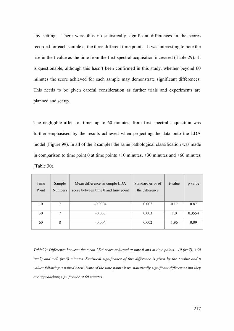
217
any setting. There were thus no statistically significant differences in the scores
recorded for each sample at the three different time points. It was interesting to note the
rise in the t value as the time from the first spectral acquisition increased (Table 29). It
is questionable, although this hasn’t been confirmed in this study, whether beyond 60
minutes the score achieved for each sample may demonstrate significant differences.
This needs to be given careful consideration as further trials and experiments are
planned and set up.
The negligible affect of time, up to 60 minutes, from first spectral acquisition was
further emphasised by the results achieved when projecting the data onto the LDA
model (Figure 99). In all of the 8 samples the same pathological classification was made
in comparison to time point 0 at time points +10 minutes, +30 minutes and +60 minutes
(Table 30).
Time
Point
Sample
Numbers
Mean difference in sample LDA
score between time 0 and time point
Standard error of
the difference
t-value
p value
10 7 -0.0004 0.002 0.17 0.87
30 7 -0.003 0.003 1.0 0.3554
60 8 -0.004 0.002 1.96 0.09
Table29: Difference between the mean LDA score achieved at time 0 and at time points +10 (n=7), +30
(n=7) and +60 (n=8) minutes. Statistical significance of this difference is given by the t value and p
values following a paired t-test. None of the time points have statistically significant differences but they
are approaching significance at 60 minutes.

218
Sample Time 0 Time 10 Time 30 Time 60
1 Neg Neg Neg Neg
2 Neg x x Neg
3 Neg Neg Neg Neg
4 Neg Neg Neg Neg
5 Neg Neg Neg Neg
6 Pos Pos Pos Pos
7 Neg Neg Neg Neg
8 Neg Neg Neg Neg
Table 30 - LDA based classification at time point 0, +10, +30 and +60 minutes. There is no difference in
any of the 8 node samples at all time points (neg=negative, pos=positive).
5.1.3 Reproducibility Experiment 1- Conclusions.
As real time clinical use of Raman spectroscopy becomes closer the results of this study
are pivotal. The vast majority of published Raman based studies to date are based on
snap frozen samples assessed within the laboratory setting. These results support the
acquisition of spectra from fresh tissue up to 60 minutes after excision. In the context of
this project this time is well beyond the time available for intra-operative analysis. As
has already been discussed this time period is approximately 40 minutes and thus these
results support the validity of results that are achieved within this time.

219
5.2. Reproducibility Experiment 2 -Use of different spectrometers.
If Raman spectroscopy driven diagnostic models are to be used clinically then it is
apparent that more than one spectrometer will need to be used. Indeed it may be that
many spectrometers are used at different sites based on a classification model derived
from one or more spectrometers. To examine the effects of using different
spectrometers a MiniRam I, a similar but earlier model of the MiniRam II was obtained
from Pacer UK, the UK distributor of B&W-Tek Raman spectrometers. This
spectrometer was then used to acquire spectra alongside the MiniRam II during 6 days
of intra-operative theatre based testing.
5.2.1. Reproducibility Experiment 2 – Methods.
To investigate the effect of using two different spectrometers an experiment protocol
was set up such that each sample could be assessed using the two systems. 5 spectra
were acquired from 14 node samples, from 9 different patients over 6 separate days in
the series described in Chapter 4. Each sample was placed on the probe and 5 spectra
were recorded using one spectrometer as described in the methods section of Chapter 4.
The collection and excitation ends of the probe were then transferred to the other
spectrometer and a further 5 spectra were obtained without moving or touching the
node. 8 nodes were assessed first with the MiniRam I and 6 with the MiniRam II to
avoid the confounding error of time. A total of 140 spectra were included in the data
analysis. All data was assessed using Matlab® software. Initial interpretation of the
results was made difficult as the computational method by which data was recorded and

220
saved by each system was slightly different and resulted in a peak shift when the raw
data was plotted. Subsequently this experiment also investigated whether the correction
methods that have previously been described (Chapter 4) would help overcome this.
PCA fed LDA was used to try and split the data based on the type of spectrometer used.
A paired t-test was then performed and finally leave one node out cross validation
testing was used to determine any differences in the classification of samples by the two
systems.
5.2.2. Reproducibility Experiment 2 – Results.
Following histopathological analysis 10 of the nodes included in this dataset were
negative; one was positive for isolated tumour cells, one for micrometastases and one
for macrometastases. As described in Chapter 4 initial spectra correction was based on
the position of the cyclohexane peaks. This helped to overcome the obvious shift that
was evident in the two groups (Figure 100, 101, 102). Despite this correction the two
groups could easily be differentiated by chemometric analysis. However the
Mahalanobis distance, which is a measure of the variability between the two groups, fell
from 4090 to 104 after this initial corrective procedure.
The second step in correcting the spectra was based on the green glass standard. The
mean green glass spectra obtained from the two spectrometers were markedly different
(Figure 103). This difference was corrected for all of the spectra acquired (Figure 104).
When PCA fed LDA was performed on this corrected dataset the Mahalanobis distance
fell further to 74.

221
400
600
800
1000
1200
1400
1600
1800
2000
4000
6000
8000
10000
12000
14000
16000
Ram
an S
hift
(cm
-1)
Intensity
Min
iRam
I
Min
iRam
II
Figure 100– Mean spectra of nodal tissue collected with two different portable Raman spectroscopy
devices (MiniRam I, n=70 (blue), MiniRam II, n=70(red)).

222
0200
400
600
800
1000
1200
1400
1600
0
0.0
2
0.0
4
0.0
6
0.0
8
0.1
0.1
2
0.1
4
0.1
6
0.1
8
0.2
Ram
an S
hift
(cm
-1)
Intensity
Min
iRam
II
Min
iRam
I
Figure 101 – Mean spectra of cyclohexane standards recorded with two different Raman spectroscopy
devices (MiniRam I, n=6 (blue), MiniRam II, n=6(red)).

223
400
600
800
1000
1200
1400
1600
1800
2000
4000
6000
8000
10000
12000
14000
16000
X: 1062
Y: 1.3
e+004
X: 1062
Y: 1.0
61e+004
X: 1299
Y: 1.0
64e+004
X: 1299
Y: 1.1
38e+004
X: 1440
Y: 1.0
58e+004
X: 1440
Y: 1.1
51e+004
X: 1652
Y: 4592
X: 1652
Y: 6520
Ram
an S
hift
(cm
-1)
Intensity
Min
iRam
II
Min
iRam
I
Figure 102 – Mean Spectra of nodal tissue recorded with the two different Raman spectroscopy devices
after shift correction (MiniRam I, n=70 (blue), MiniRam II, n=70(red)).Labels included for clarity and to
demonstrate the position of prominent peaks.

224
Figure 103 – Mean Spectra of green glass standards recorded with two different Raman spectroscopy
devices (MiniRam I, n=6(blue), MiniRam II, n=6(red)).
400
600
800
1000
1200
1400
1600
1800
0.0
05
0.0
1
0.0
15
0.0
2
0.0
25
0.0
3
0.0
35
Ram
an S
hift
(cm
-1)
Intensity
Min
iRam
I
Min
iRam
II

225
Figure 104– Mean spectra of nodal tissue collected with two different Raman spectroscopy devices after
shift correction and green glass correction (MiniRam I, n=70 (blue), MiniRam II, n=70(red)).
400
600
800
1000
1200
1400
1600
1800
2000
4000
6000
8000
10000
12000
14000
Ram
an S
hift
(cm
-1)
Intensity
Min
iRam
I
Min
iRam
II
226
Following the protocol in the previous chapter the next step involved baseline
correction the data of the data, followed by smoothing and then normalising it. After
each of these steps the Mahalanobis distance was calculated and continued to fall to 73,
64 and 26 respectively.
Following all stages of correction the mean spectra of the 14 node samples and the
cyclohexane standards collected from each spectrometer were plotted (Figure 105, 106).
The similarity of the two mean spectra was now more visible. This was supported by
the Mahalanobis distance which had fallen from 4090 to 26. Differences still remained
evident and these were highlighted when a paired t test was performed on the data.
The null hypothesis of the t-test was that there was no difference between the spectra
obtained using each spectrometer following correction. With 13 degrees of freedom the
null hypothesis would be rejected if the t value was greater than 2.65. The null
hypothesis was rejected for 35 wavenumbers suggesting that even after correcting the
data there are areas of significant difference between the spectra obtained from the two
spectrometers (Figure 107).

227
400
600
800
1000
1200
1400
1600
1800
0
0.0
1
0.0
2
0.0
3
0.0
4
0.0
5
0.0
6
0.0
7
0.0
8
0.0
9
0.1
Ram
an S
hift
(cm
-1)
Intensity
Min
iRam
II
Min
iRam
I
Figure 105 – Mean Spectra of nodal tissue recorded with two different Raman spectroscopy devices after
correction. (MiniRam I, n=70 (blue), MiniRam II, n=70(red)).

228
400
600
800
1000
1200
1400
1600
1800
0
0.0
2
0.0
4
0.0
6
0.0
8
0.1
0.1
2
0.1
4
0.1
6
0.1
8
0.2
Ram
an S
hift
(cm
-1)
Intensity
Min
iRam
I
Min
iRam
II
Figure 106 – Mean Spectra of cyclohexane standards recorded with the two different Raman
spectroscopy devices after correction (MiniRam I, n=70 (blue), MiniRam II, n=70(red)).

229
400
600
800
1000
1200
1400
1600
1800
0123456
Ram
an S
hift
(cm
-1)
t value
99%
leve
l of sta
tistical sig
nifi
cance
t va
lue for
each w
ave
num
ber
Figure 107 – Statistical significance of the residual spectral differences after correction to overcome the
use of two different Raman spectrometers (x axis = Raman Shift (cm-1), y axis = t value).

230
When these results were plotted it was clear that a significant number (24/35) of these
differences occurred in the region between 1747 and 1771 cm-1
. As detailed in Chapter
4 there were very few significant peak differences above 1747cm-1
. If the dataset was
cropped at 1748cm-1
the Mahalanobis number was further reduced to 18. Whilst
recognition of the differences was important the effect on the diagnostic outcome was
the key factor that the study hoped to demonstrate. Previous experiments, discussed in
Chapter 4, differentiating between negative v macrometastases nodes achieved a
Mahalanobis distance of 31.
Thus the differences in spectra obtained by the two spectrometers were less than the
spectral differences between the two groups. It was thus felt likely that the results from
either spectrometer could still be used to differentiate between the pathological groups.
To test this PCA fed LDA and leave one node out cross validation was used to calculate
a classification score for each sample based on the spectra collected with each
spectrometer (in a similar way to the previous experiment looking at the effects of
time). In the cross validation test the spectra from all the intra-operative node series
(n=339) that were collected with the Mini Ram II were used. The classification scores
for each sample in the series were then used to perform a paired t-test. The null
hypothesis was that there was no difference between the scores achieved using the two
systems. The null hypothesis would be rejected if the t value was greater than 2.65. The
calculated t value was 1.1281 and thus the null hypothesis was accepted. The cross
validation analysis classified each node based on the results achieved and 13/14 node
samples were placed in the same pathological category. Only one sample, a node that
had micrometastases on histopathology, was changed from a positive classification to a
negative one.

231
5.2.3. Reproducibility Experiment 2 - Conclusions
Drawing conclusions from this experiment is important for the long term viability of
Raman spectroscopy as a diagnostic tool. Although these results are drawn from a
relatively small dataset they are one of the first that directly compare spectra acquired
from human tissue in a real time clinical setting using two spectrometers. The correction
protocol, described in Chapter 4, appears to give good if not perfect spectral correction.
Although 35 of the wavenumbers show statistically significant differences only 10 of
these were between 400- 1747cm-1
which equates to 0.7% of the spectra in this region.
Data analysis in Chapter 4 did not highlight any significant peak differences between
positive and negative nodes above 1747cm-1
. Importantly there was no statistical
difference between the classification scores obtained for each node using either
spectrometer. Only one node was re-classified using the Mini Ram I. This node was in
the micrometastases group and had a classification score that placed it on the border
between the positive and negative groups. These results are therefore encouraging and
suggest that applying diagnostic models recorded with one spectrometer to prospective
data collected from multiple spectrometers could be possible. Further testing with larger
datasets and multiple spectrometers will be required prior to the clinical use of any
Raman based diagnostic model.

232
5.3. Reproducibility Experiment 3 - Multiple Users.
One of the key elements of reproducibility is that multiple users should be able to use
the equipment and still achieve the same diagnostic results. This is vital if the
spectrometer is to be used in a clinical environment by multiple users often with varying
levels of experience. An experiment was thus designed whereby three samples were
measured using the same spectrometer by 6 individuals. 1 user had extensive experience
of using the equipment, 2 had previously used the equipment on a limited basis and 3
were naïve to the system.
5.3.1. Reproducibility Experiment 3 – Methods.
In the experiment each user was given a standard instruction sheet and acquired spectra
from the three samples in the same order. They were blinded to the composition of the
samples they were measuring. 5 spectra were acquired from each sample and saved
automatically using a standard function that was built into the spectrometer. The data
was then transferred to Matlab® for further assessment. Following spectral correction
(as detailed in Chapter 4), all the spectra from each sample were plotted. PCA fed LDA
as outlined previously was employed to separate the 3 sample groups.
5.3.2. Reproducibility Experiment 3 – Results.
The spectra collected by each individual appeared broadly similar with only minimal
differences on initial inspection of each sample group (Figure 108-110).

233
PCA fed LDA was then performed to test whether the spectra recorded by each
individual could be used to differentiate the tissue into separate groups. A sensitivity
and specificity of 100% was recorded for each of the 3 groups. As can be appreciated
from reviewing the mean spectra for each sample it was much easier to differentiate the
spectra from sample c from the samples a and b (Figure 108-110). There was a degree
of variation in the spectra collected by each user but this was not significant enough to
prevent each sample being correctly grouped using PCA fed LDA (Figure 111) (Table
31). One possible explanation for these differences was a slight difference in the
position of the sample when it was placed on the probe tip. However despite this, these
results demonstrate that the equipment and technique can be used to differentiate
between different samples independent of who measured the sample.
400 600 800 1000 1200 1400 1600 18000
0.01
0.02
0.03
0.04
0.05
0.06
0.07
0.08
Raman Shift (cm-1)
Inte
nsity
Figure 108 – All spectra collected by all 6 individual users from sample A (n=30).

234
400 600 800 1000 1200 1400 1600 18000
0.01
0.02
0.03
0.04
0.05
0.06
0.07
0.08In
tensity
Raman Shift cm-1
Figure 109 – Spectra collected by all 6 individual users from sample B (n=30).
400 600 800 1000 1200 1400 1600 18000
0.05
0.1
0.15
0.2
0.25
Inte
nsity
Raman Shift (cm-1)
Figure 110 – Spectra collected by all 6 individual users from sample C (n=30).

235
Sample A
Sample B
Sample C
Sample A
30
0
0
Sample B
0
30
0
Sample C
0
0
30
Table 31- Results demonstrating 100% sensitivity and specificity independent of the assessor
Figure 111 – Separation of the three groups based on PCA fed LDA scores for all the spectra collected
by 6 different users

236
5.4 Reproducibility Experiment 3 – Conclusions.
The results presented in this chapter touch on what will in turn become a much wider
area of research. Proving that results obtained using different spectrometers by different
individuals at different times after removing the tissue from the body will be vital if this
technique is to be used as part of main stream diagnostics in breast cancer.
Much more thorough testing will of course be required to satisfy the appropriate
regulatory bodies than presented here. However these results for the first time start to
explore these concepts and as a provisional set of results they appear very promising.

237
6. Discussion
Breast cancer is a disease which attracts a great deal of clinical research, of which this
Raman based study, is one such example. There is a strong base of knowledge that
supports the use of Raman spectroscopy as a method of differentiating between normal
and malignant tissue. As systems have developed researchers have become increasingly
excited about moving the research from the laboratory to the patient’s bedside. This is
one of the first studies to take this move. By moving to the patient the study is
conducted in real time, on fresh tissue. By coupling smaller spectrometers to
mathematically based diagnostic algorithms this study supports the use of Raman
spectroscopy as a rapid, accurate, non destructive and potentially affordable diagnostic
test.
At the start of this study there were two key questions which needed to be answered.
Could a portable Raman spectrometer be used within the theatre environment and could
it achieve results at differentiating between normal and metastatic nodes that were
comparable to other modalities? If both were answered positively then the final question
would be how can the results achieved be used to take the study forward?
6.1. Could a portable Raman spectrometer be used within theatre?
Much of the clinical Raman spectroscopy work to date has been performed within the
laboratory within very stable and regulated environments. Overcoming factors

238
associated with both the operating theatre environment and the methods employed as
part of surgical technique was thus a crucial first step in this process.
Anticipated variations in temperature have been demonstrated to have a limited effect
on the spectra collected. The operating lights and ambient room lighting has been
overcome with the use of light eliminator. As it turned out, because of safety
precautions, this was not as vital as anticipated as all of the intra-operative work was
performed within a small room adjacent to theatres. None the less this work was an
important step which will allow the spectrometer to be used within theatre in the future.
One of the key concerns about any new diagnostic modality, particularly within surgical
oncology, is the importance of avoiding cross contamination. The devastating effects of
one patient undergoing, ultimately unnecessary, treatment based on the results of
another patient must be avoided. This study utilised two different mechanisms to avoid
this. The first and most important of these was ensuring that all node assessment was
performed before the patient left the operating theatre. The second technique was the
use of a sterile sheath. Early testing demonstrated that this had minimal effect on the
spectra collected and was thus used throughout the clinical phase of this study.
The time taken to collect spectra and thus “assess” the node is not only critical to avoid
clinical errors but is also important when considering the ultimate aim of guiding a
clinical decision as to the need for an axillary clearance. An intra-operative test needs to
provide results in a time frame that avoids any delays that would disrupt an operating
list and mean that the patient is anaesthetised for a longer period of time than necessary.

239
Current techniques are performed on the excised node whilst the operating surgeon
continues with the excision of the breast tumour. If an axillary clearance is deemed to be
required then this is performed as the final part of the operation. Within this study no
patient underwent further axillary surgery based on the results of either the Raman
spectrometer or any other intra-operative method. Ensuring that all assessment took
place before the patient left theatre, initially to prevent cross-contamination of samples,
also demonstrated that the results could be delivered without undue delay if an axillary
dissection was deemed necessary. It can be argued that the “assessment” carried out in
this study was not complete as there was no diagnostic output, but it is anticipated that
algorithms used to provide this answer will be rapid and measured in seconds.
The time frame of assessment took on further importance when the effects of time post
excision of tissue were investigated. The results of the reproducibility study looking at
the effects of time post excision suggest that there are no statistically significant
differences up to 60 minutes after tissue removal. The trend in the t-value does however
suggest that this may not be the case much beyond this time frame, and will need to be
considered when planning future studies.
Introducing a new step in the management of a particular condition requires that the
additional step is compatible with the established techniques. One of the concerns at the
outset of the study was the effect of Patent V blue dye on the spectra obtained from the
lymph nodes. Within the UK this dye is widely used to help identify the lymph node
and any new test will need to be compatible with it. Although initial studies suggested
that this was likely to be problematic, further studies on nodes in the Dudley series

240
disproved this. The identification of the principal component of blue dye and its
subsequent removal from reconstituted spectra had little effect on the diagnostic
potential of the results achieved. One potential problem as this project moves forward is
that, although blue dye is widely used in the UK, other markers such as Indomethacin
Green are used elsewhere and this will need to be accounted for.
6.2. Could a portable Raman probe achieve results at differentiating between
normal and metastatic nodes that were comparable to other modalities?
In any clinically based study the “buy-in” of the clinicians whose patients you hope to
recruit is vital. Before embarking on real time clinical work it was important to
demonstrate to them why a diagnostic test based on Raman spectroscopy might work.
This involves both a study of the previously published literature and early feasibility
studies using the equipment that we had selected.
Previous work, as discussed in Chapter 2, has consistently shown, within breast tissue,
that the key differences in the spectra obtained are an increased contribution of lipid in
the normal tissue relative to an increased contribution of protein and DNA in the
malignant tissue. These results are supported by FTIR studies in axillary, oesophageal
and head and neck cancers, and by mapping Raman studies on axillary lymph nodes
performed within our own unit (Smith 2005). The mapping studies and subsequent
probe modelling of the data produced were carried out on tissue with a depth of several
μm. To replicate this tissue depth in this study would have involved a significant
preparatory step. This would have extended the time frame beyond clinical relevance

241
and potentially damaged tissue that remained important for the staging and thus
management planning of the patients who agreed to take part in the study. A number of
experiments were set up to estimate the depth from which spectral information could be
collected using the MiniRam II spectrometer and probe. Whilst it is recognised that
there are a number of limitations to these studies and that interpretation should therefore
be performed with caution the results suggest that spectral information could be
detected at depths up to 3mm. This was crucial as the vast majority of lymph nodes
have been shown to be less than 9mm in diameter and metastatic deposits are initially
found within the medulla of the node before spreading to the cortex. By collecting
spectra from the inner surface there was confidence that spectral information
particularly related to macrometastases would be detected if they were present.
Prior to commencing studies within theatre a feasibility study was performed on node
samples that had been collected by collaborators at Russell’s Hall Hospital, Dudley,
UK. The feasibility study, discussed in Chapter 3, included 38 node samples from 17
different patients and revealed very encouraging results. A sensitivity of up to 90% and
a specificity of up to 96% were achieved using unsupervised leave one node out testing.
The results achieved were broadly similar even when only 5 spectra were assessed per
node and enabled the “assessment” of each node to be performed in a clinically relevant
time frame. There were a number of drawbacks to this study however. The samples
were snap frozen, it was often difficult to determine the orientation of the node and thus
definitively collect spectra from the inner half, and the “gold standard”
histopathological assessment was based on a single slice with immuno-histochemistry
staining. Therefore spectra may have been collected from the outer half of the node and

242
samples may have been mis-classified. It was however an important step in establishing
the potential of the equipment we were using and it was hoped that even better results
could be achieved in the real time study.
Building on both the feasibility study and the preparatory experimentation the clinically
based part of this study was established. With local ethical approval a total of 66
patients undergoing 72 operative procedures were recruited and from these patients 339
samples from 176 lymph nodes were assessed. The results achieved when trying to
distinguish between the two most distinct groups, the macrometastases and the N0
patients were most promising, as discussed in Chapter 4. The unsupervised test result
achieved specificity of 99.4% and a sensitivity of 93.8%, which is easily comparable if
not far better than currently available intra-operative tests. Evidence that these results
are based on differences in lipid, protein and DNA contributions is also consistent with
previous work on breast cancer and normal breast tissue and is vital in helping explain
the application of the test to clinicians. On an individual level 44/48 patients would have
benefited from intraoperative testing had the results been used to guide clinical decision
making. In particular 38 patients would have been spared the wait for their
histopathological nodal assessment, and 6 would have avoided the need for a second
operation to clear the axilla. There would have been two false positives and this will
need to be addressed as the use of Raman spectroscopy moves forward. It is vital that
the specificity should be maintained as close to 100% as possible, as the result of a false
positive would be a recommendation for an axillary clearance that ultimately was not
needed.

243
The subsequent inclusion of negative nodes from non-N0 patients into the negative
group had a deleterious effect on the specificity (96%) and sensitivity (84%). This is
suggestive that there are some differences within nodes that although not metastatic
themselves are part of a chain of nodes at least one of which is metastatic. Peak analysis
demonstrated significant differences in the contribution of proteins to the spectra of
non-N0 nodes. This may have affected the overall classification model and could
account for the increase in both false negatives and false positives. For the individual
patient involved this would not have had any deleterious effects as they would, by
definition, have had another node that was positive. They would therefore already have
been defined as having a positive axilla.
The effect of these non-N0 negative nodes is important in helping to design a
mathematical algorithm as this project progresses forward. This data suggest that any
such algorithm will need to be based on spectra from N0 patients only and not negative
nodes from non-N0 patients.
In comparison to the results achieved with the macrometastases the results from the
nodes with either micrometastases, 50% sensitivity, or isolated tumour cells, 40%
sensitivity, were disappointing. It was interesting to note that those that were
successfully identified and those that were not, appeared to be in two distinct groups
based on the contribution of lipid, protein and DNA to the spectra. It could be argued
therefore that within the samples which were correctly identified the foci of metastases
did significantly contribute to the spectra but in the other samples it either did not at all
(i.e. it was not “seen”) or the greater amount of normal tissue eclipsed it. This may be a

244
reflection on the small size of the deposits within the tissue and the difficulty detecting
them using the methodology that was employed. If it was clinically felt that the
identification of micrometastases and isolated tumour cells remained important then
samples used in future studies may need to be multiply sectioned before spectra were
acquired to help overcome this problem. The emerging data, especially from Z-0011
suggests that this is unlikely to be the case. It is likely that patients with ITCs will
continue to be classified as node negative and that those with micrometastases will
increasingly not be recommended to undergo further axillary surgery. If further surgery
is recommended then this should be following MDT discussion and would not, given
the current evidence, be following intra-operative assessment.
In situ testing from the outer surface of the node was suggested as a possible next step
forward for this project. However the results presented, a fall in sensitivity to 81% for
the identification of macrometastases, do not support this. The difference can be
explained by the initial presence of metastatic deposits within the medulla before spread
towards the cortex occurs. Therefore by placing the probe on the outer surface, light will
be scattered first by a normal cortex before it reaches a metastatic medulla. No
improvements in the results for the micrometastases or isolated tumour cells were
reported. Thus future testing should continue to collect spectra from the cut inner half of
the node.

245
6.3. Future Studies
The results presented within this thesis really do open the door to real time “bed side”
tissue testing using Raman spectroscopy. This technique which is quick, non destructive
(thus facilitating gold standard cross checking) and affordable has many advantages
over the other currently available methodologies that were outlined in Chapter 1. Before
it can guide clinical management a number of future studies need to be completed.
The first and most important next step should be the production of a classification
algorithm or model that can then be prospectively tested. It is envisaged that this model
would be based on dataset 1 that was discussed in Chapter 4. Prospectively testing this
with independent specimens could then directly compare Raman spectroscopy and its
algorithmic model to the current gold standard. Particular care will be need to be paid to
any false positive results as these are the cases that need to be avoided. Further
sectioning of the axillary node by the pathologists may be required to ensure that the
gold standard technique hasn’t missed any small deposits that the Raman device is
“seeing”. Initially this testing would be take place at one hospital site but then latterly
this could be extended to multiple units, with multiple spectrometers. The use of
multiple instruments and users would build on the reproducibility experiments outline in
Chapter 5. The results from these independent samples could then be added to the
algorithm to further increase its size and robusticity. It is hoped that with increasing
sample numbers the classification model will become more powerful resulting in further
improvements in sensitivity and specificity. This work is ongoing currently and the
results are awaited eagerly. It is hoped that these results will provide a catalyst for

246
further studies that move Raman spectroscopy away from the laboratory to the patient’s
bed side. Within breast cancer the demonstration that this equipment can differentiate
between normal and metastatic tissue opens it up to use in the immediate assessment of
core biopsy samples, within a “one-stop” breast clinic or the interrogation of margin
status during a wide local excision. Outside of breast cancer the potential for Raman
spectroscopy to be used in a wide range of clinical scenarios is very real. It could, for
example, be used in place of frozen section analysis in parathyroid or anal surgery by
giving an immediate assessment of tissue type.
6.4 Conclusions
This study has taken a very important step toward the clinical use of Raman
spectroscopy to improve patient care. After many years of offering great potential its
use within a real-time clinical situation has been demonstrated. At the start of Chapter 2
a table demonstrating the key features of a diagnostic tool for use in intra-operative
axillary node testing was shown. The ideal technology needed to be sensitive and
specific, usable within the theatre environment, fast, cost effective and non destructive.
No currently available method of node assessment offers all of these features. This
study has shown that Raman spectroscopy can and does meet all these criteria. Further
work to develop and test a diagnostic algorithm and to enhance on the reproducibility
studies described in Chapter 5 will be required, but the use of Raman spectroscopy to
improve the lives of patients with breast cancer is now within touching distance.

247
7.Bibliography
Alfano, R. R., Das, B. B., Cleary, J., Prudente, R. and Celmer, E. J. (1991), "Light sheds
light on cancer--distinguishing malignant tumors from benign tissues and
tumors", Bulletin of the New York Academy of Medicine, vol. 67, no. 2, pp. 143-
150.
Allweis, T. M., Kaufman, Z., Lelcuk, S., Pappo, I., Karni, T., Schneebaum, S., Spector,
R., Schindel, A., Hershko, D., Zilberman, M., Sayfan, J., Berlin, Y., Hadary, A.,
Olsha, O., Paran, H., Gutman, M. and Carmon, M. (2008), "A prospective,
randomized, controlled, multicenter study of a real-time, intraoperative probe for
positive margin detection in breast-conserving surgery", American Journal of
Surgery, vol. 196, no. 4, pp. 483-489.
Alvarez, S., Anorbe, E., Alcorta, P., Lopez, F., Alonso, I. and Cortes, J. (2006), "Role of
sonography in the diagnosis of axillary lymph node metastases in breast cancer:
a systematic review", American Journal of Roentgenology, vol. 186, no. 5, pp.
1342-1348
Beattie, J. R., Bell, S. E., Borgaard, C., Fearon, A. and Moss, B. W. (2006), "Prediction
of adipose tissue composition using Raman spectroscopy: average properties and
individual fatty acids", Lipids, vol. 41, no. 3, pp. 287-294.
Beattie, J. R., Bell, S. E., Borggaard, C., Fearon, A. M. and Moss, B. W. (2007),
"Classification of adipose tissue species using Raman spectroscopy", Lipids, vol.
42, no. 7, pp. 679-685.
Benson, J. R. and Wishart, G. C. (2010), "Is intra-operative nodal assessment essential
in a modern breast practice?", European Journal of Surgical Oncology, vol. 36,
no. 12, pp. 1162-1164.
Berry, E. and Kohn, M. (2000), Operating Room Technique, 9th ed, Mosby,
Philadelphia.
Bilimoria, K. Y., Bentrem, D. J., Hansen, N. M., Bethke, K. P., Rademaker, A. W., Ko,
C. Y., Winchester, D. P. and Winchester, D. J. (2009), "Comparison of sentinel
lymph node biopsy alone and completion axillary lymph node dissection for
node-positive breast cancer", Journal of Clinical Oncology, vol. 27, no. 18, pp.
2946-2953.
Bird, B., Romeo, M., Laver, N. and Diem, M. (2009), "Spectral detection of micro-
metastases in lymph node histo-pathology", Journal of Biophotonics, vol. 2, no.
1-2, pp. 37-46.
Bleiweiss, I. J., Nagi, C. S. and Jaffer, S. (2006), "Axillary sentinel lymph nodes can be
falsely positive due to iatrogenic displacement and transport of benign epithelial
cells in patients with breast carcinoma", Journal of Clinical Oncology, vol. 24,
no. 13, pp. 2013-2018.

248
Blumencranz, P., Whitworth, P. W., Deck, K., Rosenberg, A., Reintgen, D., Beitsch, P.,
Chagpar, A., Julian, T., Saha, S., Mamounas, E., Giuliano, A. and Simmons, R.
(2007), "Scientific Impact Recognition Award. Sentinel node staging for breast
cancer: intraoperative molecular pathology overcomes conventional histologic
sampling errors", American Journal of Surgery, vol. 194, no. 4, pp. 426-432.
Brock, L. (1975), "The importance of environmental conditions, especially temperature,
in the operating room and intensive care ward", British Journal of Surgery, vol.
62, no. 4, pp. 253-258.
Burger, L. and Fitzpatrick, J. (2009), "Prevention of inadvertent perioperative
hypothermia", British Journal of Nursing, vol. 18, no. 18, pp. 1114, 1116-9.
Burke, M. and Seeters, J. (2010) Breast Lymph Node Assay: Headline Report. York
Health Economics Consortium and NHS Technology Adoption Centre (NTAC)
Available at: www.ntac.nhs.uk [ Accessed Jan 2010].
Cacaecu, T. (2008), Spleen and Other Lymphatic Organs, available at:
http://education.vetmed.vt.edu/curriculum/vm8054/labs/Lab13/IMAGES/LYMP
H%20NODE%20LOW%201.jpg [Accessed January 2010].
Cancer Research UK (2009), TNM Breast Cancer Staging, available at:
http://www.cancerhelp.org.uk/type/breast-cancer/treatment/tnm-breast-cancer-
staging [Accessed January 2010].
Cancer Research UK (2011), Breast Cancer UK Statistics. Available at:
http://info.cancerresearchuk.org/cancerstats/types/breast/incidence
(Accessed March 2011).
Carter, B. A., Jensen, R. A., Simpson, J. F. and Page, D. L. (2000), "Benign transport of
breast epithelium into axillary lymph nodes after biopsy", American Journal of
Clinical Pathology, vol. 113, no. 2, pp. 259-265.
Chao, C. (2004), "The use of frozen section and immunohistochemistry for sentinel
lymph node biopsy in breast cancer", The American Surgeon, vol. 70, no. 5, pp.
414-419.
Chicken, D. W., Sivanadarajah, N. and Keshtgar, M. R. (2007), "Patients' view on
intraoperative diagnosis of sentinel nodes in breast cancer: is it an automatic
choice?", International Journal of Surgery, vol. 5, no. 2, pp. 76-80.
Chowdary, M. V., Kumar, K. K., Kurien, J., Mathew, S. and Krishna, C. M. (2006),
"Discrimination of normal, benign, and malignant breast tissues by Raman
spectroscopy", Biopolymers, vol. 83, no. 5, pp. 556-569.
Chowdary, M. V., Kalyan Kumar, K., Mathew, S., Rao, L., Krishna, C. M. and Kurien,
J. (2009), "Biochemical correlation of Raman spectra of normal, benign and

249
malignant breast tissues: a spectral deconvolution study", Biopolymers, vol. 91,
no. 7, pp. 539-546.
Cooper, K. L., Harnan, S., Meng, Y., Ward, S. E., Fitzgerald, P., Papaioannou, D.,
Wyld, L., Ingram, C., Wilkinson, I. D. and Lorenz, E. (2011), "Positron
emission tomography (PET) for assessment of axillary lymph node status in
early breast cancer: A systematic review and meta-analysis", European Journal
of Surgical Oncology vol. 37, no. 3, pp. 187-198.
Cote,R., Giuliano,A.E., Hawes,D., Ballman,K.V., Whitworth.D., Blumencranz,
P.,Reintgen,D., Morrow,M., Leitch,A.M.,Hunt,K. (2010), "ACOSOG Z0010: A
multicenter prognostic study of sentinel node (SN) and bone marrow (BM)
micrometastases in women with clinical T1/T2 N0 M0 breast cancer", Journal
of Clinical Oncology, Vol. 28:18s, (suppl; abstr CRA504).
Creager, A. J. and Geisinger, K. R. (2002), "Intraoperative evaluation of sentinel lymph
nodes for breast carcinoma: current methodologies", Advances in Anatomic
Pathology, vol. 9, no. 4, pp. 233-243.
Cserni, G., Amendoeira, I., Apostolikas, N., Bellocq, J. P., Bianchi, S., Bussolati, G.,
Boecker, W., Borisch, B., Connolly, C. E., Decker, T., Dervan, P., Drijkoningen,
M., Ellis, I. O., Elston, C. W., Eusebi, V., Faverly, D., Heikkila, P., Holland, R.,
Kerner, H., Kulka, J., Jacquemier, J., Lacerda, M., Martinez-Penuela, J., De
Miguel, C., Peterse, J. L., Rank, F., Regitnig, P., Reiner, A., Sapino, A., Sigal-
Zafrani, B., Tanous, A. M., Thorstenson, S., Zozaya, E., Wells, C. A. and
European Working Group for Breast Screening Pathology (2003), "Pathological
work-up of sentinel lymph nodes in breast cancer. Review of current data to be
considered for the formulation of guidelines", European Journal of Cancer , vol.
39, no. 12, pp. 1654-1667.
Damera, A., Evans, A. J., Cornford, E. J., Wilson, A. R., Burrell, H. C., James, J. J.,
Pinder, S. E., Ellis, I. O., Lee, A. H. and Macmillan, R. D. (2003), "Diagnosis of
axillary nodal metastases by ultrasound-guided core biopsy in primary operable
breast cancer", British Journal of Cancer, vol. 89, no. 7, pp. 1310-1313.
Das, K., Kendall, C., Isabelle, M., Fowler, C., Christie-Brown, J. and Stone, N. (2008),
"FTIR of touch imprint cytology: A novel tissue diagnostic technique", Journal
of Photochemistry and Photobiology B: Biology, vol. 92, no. 3, pp. 160-164.
de Boer, M., van Deurzen,C.H, van Dijck, J.A, Borm,G.F., Diest,P.J., Adang, E.M.,
Nortier,J.W.R,. Rutgers, E.J., Seynaeve, C., Menke-Pluymers, M., Bult, P. and
Tjan-Heijnen V.C. (2009) " Micrometastases or Isolated Tumor Cells and the
Outcome of Breast Cancer" New England Journal of Medicine vol. 361, no. 7
pp.653-663.
de Boer, M., van Dijck, J. A., Bult, P., Borm, G. F. and Tjan-Heijnen, V. C. (2010),
"Breast cancer prognosis and occult lymph node metastases, isolated tumor
250
cells, and micrometastases", Journal of the National Cancer Institute, vol. 102,
no. 6, pp. 410-425.
Diem, M., Chalmers, JM. and Griffiths, PR. ( 2008). Vibrational spectroscopy for
medical diagnosis. 1st Edition , John Wiley and Sons 2008.
DoITPoMS, University of Cambridge, UK. Raman Spectroscopy. (2010) Available
from: http://www.doitpoms.ac.uk/tlplib/raman/index.php [Accessed October
2010]
Early Breast Cancer Trialists' Collaborative Group (EBCTCG) (2005), "Effects of
chemotherapy and hormonal therapy for early breast cancer on recurrence and
15-year survival: an overview of the randomised trials", Lancet, vol. 365, no.
9472, pp. 1687-1717.
Ellis, H. (2002), Clinical Anatomy, 10th ed, Wiley Blackwell, 2002.
Ellis, H. (2003). Anatomy of the Breast. In Surgery- The Continuously Updated
Textbook of Surgery (CD-ROM). London, UK: The Medicine Publishing
Company Ltd.
Elmore, S. A. (2006), "Histopathology of the lymph nodes", Toxicologic Pathology, vol.
34, no. 5, pp. 425-454.
Elston, C. W. and Ellis, I. O. (1991), "Pathological prognostic factors in breast cancer. I.
The value of histological grade in breast cancer: experience from a large study
with long-term follow-up", Histopathology, vol. 19, no. 5, pp. 403-410.
Frank, C.J., McCreery, R L., Redd, D.C, and Gansler, T.S,.(1993) "Detection of
Silicone in Lymph Node Biopsy Specimens by Near-Infrared Raman
Spectroscopy", Applied Spectroscopy Vol 47 no. 4, pp. 387-390.
Frank, C. J., McCreery, R. L. and Redd, D. C. (1995), "Raman spectroscopy of normal
and diseased human breast tissues", Analytical Chemistry, vol. 67, no. 5, pp.
777-783.
Gelmon, K. A. (2010), "The ongoing debate about nodes", Clinical Breast Cancer, vol.
10, no. 4, pp. 265-266.
Giuliano, A. E., Kirgan, D. M., Guenther, J. M. and Morton, D. L. (1994), "Lymphatic
mapping and sentinel lymphadenectomy for breast cancer", Annals of Surgery,
vol. 220, no. 3, pp. 391-8; discussion 398-401.
Giuliano, A. E., McCall, L., Beitsch, P., Whitworth, P. W., Blumencranz, P., Leitch, A.
M., Saha, S., Hunt, K. K., Morrow, M. and Ballman, K. (2010), "Locoregional
recurrence after sentinel lymph node dissection with or without axillary
dissection in patients with sentinel lymph node metastases: the American

251
College of Surgeons Oncology Group Z0011 randomized trial", Annals of
Surgery, vol. 252, no. 3, pp. 426-32; discussion 432-3.
Giuliano, A. E., Hunt, K. K., Ballman, K. V., Beitsch, P. D., Whitworth, P. W.,
Blumencranz, P. W., Leitch, A. M., Saha, S., McCall, L. M. and Morrow, M.
(2011), "Axillary dissection vs no axillary dissection in women with invasive
breast cancer and sentinel node metastasis: a randomized clinical trial", Journal
of the American Medical Association, vol. 305, no. 6, pp. 569-575.
Goyal, A. and Mansel, R. E. (2008), "Recent advances in sentinel lymph node biopsy
for breast cancer", Current Opinion in Oncology, vol. 20, no. 6, pp. 621-626.
Haka, A. S., Shafer-Peltier, K. E., Fitzmaurice, M., Crowe, J., Dasari, R. R. and Feld,
M. S. (2005), "Diagnosing breast cancer by using Raman spectroscopy",
Proceedings of the National Academy of Sciences of the United States of
America, vol. 102, no. 35, pp. 12371-12376.
Haka, A. S., Volynskaya, Z., Gardecki, J. A., Nazemi, J., Lyons, J., Hicks, D.,
Fitzmaurice, M., Dasari, R. R., Crowe, J. P. and Feld, M. S. (2006), "In vivo
margin assessment during partial mastectomy breast surgery using raman
spectroscopy", Cancer Research, vol. 66, no. 6, pp. 3317-3322.
Haka, A. S., Volynskaya, Z., Gardecki, J. A., Nazemi, J., Shenk, R., Wang, N., Dasari,
R. R., Fitzmaurice, M. and Feld, M. S. (2009), "Diagnosing breast cancer using
Raman spectroscopy: prospective analysis", Journal of Biomedical Optics, vol.
14, no. 5, pp. 054023.
Hejmadi, M. (2010), An Introduction to Cancer Biology, Verntus Publishing
Available from: http://web.mef.hr/web/images/pdf/int_canc_b.pdf [Accessed
April 2011]
Hirsch, J. I., Banks, W. L.,Jr, Sullivan, J. S. and Horsley, J. S.,3rd (1989), "Effect of
methylene blue on estrogen-receptor activity", Radiology, vol. 171, no. 1, pp.
105-107.
Hollas, J. M. (2005), Modern Spectroscopy, 5th ed, John Wiley and Sons, London.
Horsnell, J., Smith, J., Sattlecker, M., Sammon, A., Christie-Brown, J., Kendall, C. and
Stone, N. (2011) "Raman Spectroscopy, a potential new method for the intra-
operative assessment of axillary lymph nodes" The Surgeon,
doi:10.1016/j.surge.2011.02.004.
Horsnell, J., Knight, H., Court, F., Chan, C., Bristol, J. (2012) "Intra-operative Sentinel
Lymph Node Assessment - How many patients will avoid a second operation?"
European Journal of Surgical Oncology, Vol. 38, no. 5, pp 459-460.
Ioachim, H. L. and Ratech, H. (2002), Ioachim's Lymph Node Pathology, 3rd ed,
Lippincott Williams & Wilkins, Philapdelphia, PA 19106 USA.

252
Isabelle,M., Stone,N., Barr,H., Vipond,M. Shepherd,N. and Rogers, K. (2008), "Lymph
Node Pathology using Optical Spectroscopy in Lymph Node diagnostics"
Spectroscopy, vol.22, no. 2-3, pp 97-104.
Johnson, K. S., Chicken, D. W., Pickard, D. C. O., Lee, A. C., Briggs, G., Falzon, M.,
Bigio, I. J., Keshtgar, M. R. and Bown, S. G. (2004), "Elastic scattering
spectroscopy for intraoperative determination of sentinel lymph node status in
the breast", Journal of Biomedical Optics, vol. 9, no. 6, pp. 1122-1128.
Johnstone, S. (2002), International Handbook of Breast Cancer, 1st ed, Euromed
Communications Ltd., Haslemere.
Katzin, W. E., Centeno, J. A., Feng, L. J., Kiley, M. and Mullick, F. G. (2005),
"Pathology of lymph nodes from patients with breast implants: a histologic and
spectroscopic evaluation", American Journal of Surgical Pathology, vol. 29,
no. 4, pp. 506-511.
Keller, M.D., Majumder, S. K and Mahadevan-Jansen, A. (2009) "Spatially offset
Raman spectroscopy of layered soft tissues", Optics Letters, vol. 34 no.7,
pp.926-928.
Keller, M, D., Wilson, R., Mycek, M. and Mahadevan-Jansen, A. (2010) "Monte Carlo
Model of Spatially Offset Raman Spectroscopy for Breast Tumor Margin
Analysis" Applied Spectroscopy vol. 64, no.6, pp. 607-614.
Kendall, C. (2002), A Study of Raman spectroscopy for the early detetction and
classification of malignancy in oesophageal tissue (unpublished PhD. thesis),
Cranfield University, UK, Cranfield, UK.
Kendall, C., Stone, N., Shepherd, N., Geboes, K., Warren, B., Bennett, R. and Barr, H.
(2003), "Raman spectroscopy, a potential tool for the objective identification and
classification of neoplasia in Barrett's oesophagus", Journal of Pathology, vol.
200, no. 5, pp. 602-609.
Kerssens, M. M., Matousek, P., Rogers, K. and Stone, N. (2010), "Towards a safe non-
invasive method for evaluating the carbonate substitution levels of
hydroxyapatite (HAP) in micro-calcifications found in breast tissue", The
Analyst, vol. 135, no. 12, pp. 3156-3161.
Keshtgar, M. R. (2009), "Intra-operative assessment of sentinel nodes", in Sibbering, M.
(ed.) The Association of Breast Surgery at BASO Yearbook 2009, ABS at BASO,
London WC2A 3PE, pp. 62-65.
Keshtgar, M. R., Chicken, D. W., Austwick, M. R., Somasundaram, S. K., Mosse, C.
A., Zhu, Y., Bigio, I. J. and Bown, S. G. (2010), "Optical scanning for rapid
intraoperative diagnosis of sentinel node metastases in breast cancer",
British Journal of Surgery, vol. 97, no. 8, pp. 1232-1239.

253
Kim, T., Giuliano, A. E. and Lyman, G. H. (2006), "Lymphatic mapping and sentinel
lymph node biopsy in early-stage breast carcinoma: a meta-analysis", Cancer,
vol. 106, no. 1, pp. 4-16.
Krag, D. N., Weaver, D. L., Alex, J. C. and Fairbank, J. T. (1993), "Surgical resection
and radiolocalization of the sentinel lymph node in breast cancer using a gamma
probe", Surgical Oncology, vol. 2, no. 6, pp. 335-9; discussion 340.
Kuby, J. (1997), Immunology, 3rd ed, Freeman and Company, New York.
Kurosumi, M. and Takei, H. (2007), "Significance and problems of histopathological
examination and utility of real-time reverse transcriptase-polymerase chain
reaction method for the detection of sentinel lymph node metastasis in breast
cancer", Breast Cancer, vol. 14, no. 4, pp. 342-349.
Layfield, D. M., Agrawal, A., Roche, H. and Cutress, R. I. (2011), "Intraoperative
assessment of sentinel lymph nodes in breast cancer", British Journal of
Surgery, vol. 98, no. 1, pp. 4-17.
Lim, S.M. and Lam, F.L. (2005), "Laparoscopic-assisted axillary dissection in breast
cancer surgery", American Journal of Surgery, vol.190, no.4, pp. 641-643.
Loftus P. (2010) "Doctors thought discontinued J&J cancer test was impractical."
http://online.wsj.com/article/BT-CO-20100125-710277.html. The Wall Street
Journal 25 January 2010.
Lovat, L. B., Johnson, K., Mackenzie, G. D., Clark, B. R., Novelli, M. R., Davies, S.,
O'Donovan, M., Selvasekar, C., Thorpe, S. M., Pickard, D., Fitzgerald, R.,
Fearn, T., Bigio, I. and Bown, S. G. (2006), "Elastic scattering spectroscopy
accurately detects high grade dysplasia and cancer in Barrett's oesophagus", Gut,
vol. 55, no. 8, pp. 1078-1083.
Mangram, A. J., Horan, T. C., Pearson, M. L., Silver, L. C. and Jarvis, W. R. (1999),
"Guideline for Prevention of Surgical Site Infection, 1999. Centers for Disease
Control and Prevention (CDC) Hospital Infection Control Practices Advisory
Committee", American Journal of Infection Control, vol. 27, no. 2, pp. 97-132;
quiz 133-4; discussion 96.
Manoharan, R., Shafer, K., Perelman, L., Wu, J., Chen, K., Deinum, G., Fitzmaurice,
M., Myles, J., Crowe, J., Dasari, R. R. and Feld, M. S. (1998), "Raman
spectroscopy and fluorescence photon migration for breast cancer diagnosis and
imaging", Photochemistry and Photobiology, vol. 67, no. 1, pp. 15-22.
Mansel, R. E., Fallowfield, L., Kissin, M., Goyal, A., Newcombe, R. G., Dixon, J. M.,
Yiangou, C., Horgan, K., Bundred, N., Monypenny, I., England, D., Sibbering,
M., Abdullah, T. I., Barr, L., Chetty, U., Sinnett, D. H., Fleissig, A., Clarke, D.
and Ell, P. J. (2006), "Randomized multicenter trial of sentinel node biopsy

254
versus standard axillary treatment in operable breast cancer: the ALMANAC
Trial", Journal of the National Cancer Institute, vol. 98, no. 9, pp. 599-609.
Matern, U. and Koneczny, S. (2007), "Safety, hazards and ergonomics in the operating
room", Surgical Endoscopy, vol. 21, no. 11, pp. 1965-1969.
Matousek, P. and Stone, N. (2007), "Prospects for the diagnosis of breast cancer by
non-invasive probing of calcifications using transmission Raman spectroscopy",
Journal of Biomedical Optics, vol. 12, no. 2, doi.10.1117/1.2718934
Molckovsky, A., Song, L. M., Shim, M. G., Marcon, N. E. and Wilson, B. C. (2003),
"Diagnostic potential of near-infrared Raman spectroscopy in the colon:
differentiating adenomatous from hyperplastic polyps", Gastrointestinal
Endoscopy, vol. 57, no. 3, pp. 396-402.
Moore, K. A., A. (2005), Essential Clinical Anatomy, 3rd Edition ed., Lippincott
Williams & Wilkins, London.
National Comprehensive Cancer Network (2012), "Clinical Practice Guidelines in
Oncology. Breast Cancer" National Comprehensive Cancer Network Inc
available at: www.nccn.org. [Accessed April 2012]
National Institute for Health and Clinical Excellence (February 2009), "Early and
locally advanced breast cancer", Clinical Guideline 80, National Institute for
Health and Clinical Excellence, London WC1V 6NA.
NHS Breast Screening Programme (2008), Annual Review: Saving Lives through
Screening NHSBSP, National Health Service, UK, London, UK.
NHS Cancer Screening Programmes and West Midlands Cancer Intelligence Unit
(2009), An Audit of Screen Detected Breast Cancers for the Year of Screening
April 2007 to March 2008, NHSBSP, National Health Service, UK, London,
UK.
Obwegeser, R., Lorenz, K., Hohlagschwandtner, M., Czerwenka, K., Schneider, B. and
Kubista, E. (2000), "Axillary lymph nodes in breast cancer: is size related to
metastatic involvement?” World Journal of Surgery, vol. 24, no. 5, pp. 546-550.
Paik, S., Tang, G., Shak, S., Kim, C., Baker, J., Kim, W., Cronin, M., Baehner, F. L.,
Watson, D., Bryant, J., Costantino, J. P., Geyer, C. E.,Jr, Wickerham, D. L. and
Wolmark, N. (2006), "Gene expression and benefit of chemotherapy in women
with node-negative, estrogen receptor-positive breast cancer", Journal of
Clinical Oncology, vol. 24, no. 23, pp. 3726-3734.
Patani, N., Cutuli, B. and Mokbel, K. (2008), "Current management of DCIS: a review",
Breast Cancer Research and Treatment, vol. 111, no. 1, pp. 1-10.

255
Pinder, S. (2009), "Sentinel Node Biopsy Pathology", in Sibbering, M. (ed.) The
Association of Breast Surgery at BASO Yearbook 2009, ABS at BASO, London
WC2A 3PE, pp. 66-69.
Pond, C. M. and Mattacks, C. A. (2003), "The source of fatty acids incorporated into
proliferating lymphoid cells in immune-stimulated lymph nodes", British
Journal of Nutrition, vol. 89, no. 3, pp. 375-382.
Purushotham, A. D., Upponi, S., Klevesath, M. B., Bobrow, L., Millar, K., Myles, J. P.
and Duffy, S. W. (2005), "Morbidity after sentinel lymph node biopsy in
primary breast cancer: results from a randomized controlled trial", Journal of
Clinical Oncology, vol. 23, no. 19, pp. 4312-4321.
Quan, M. L. and McCready, D. (2009), "The evolution of lymph node assessment in
breast cancer", Journal of Surgical Oncology, vol. 99, no. 4, pp. 194-198.
Raftery, A. (ed.) (2000), Applied Basic Science for Basic Surgical Training, Illustrated
Edition ed, Churchill Livingstone, London.
Redd, D. C., Feng, C., Yue, K. and Gansler, T. S. (1993), "Raman Spectroscopic
Characterization of Human Breast Tissues: Implications for Breast Cancer
Diagnosis", Applied Spectroscopy, vol. 47, no. 6, pp. 787-791.
Rhakha, E., El-Sayed, M. and Powe, D. (2008), "Invasive Lobular Carcinoma of the
Breast: Response to hormonal therapy and outcome", European Journal of
Cancer, vol.44, no.1, pp73-83.
Rosen, P. P. (2001), Rosen's Breast Pathology, 2nd ed, Lippincott Williams and
Wilkins, Philadelphia.
Rovera, F., Frattini, F., Marelli, M., Corben, A. D., Dionigi, G., Boni, L. and Dionigi, R.
(2008), "Axillary sentinel lymph node biopsy: an overview", International
Journal of Surgery, vol. 6 Suppl 1, pp. S109-12.
Sabel, M. S. (2009), Essentials of Breast Surgery, 1st ed, Mosby Elsevier, Philadelphia.
Sakr, R., Barranger, E., Antoine, M., Prugnolle, H., Darai, E. and Uzan, S. (2006),
"Ductal carcinoma in situ: value of sentinel lymph node biopsy", Journal of
Surgical Oncology, vol. 94, no. 5, pp 426-430.
Sant, M., Francisci, S., Capocaccia, R., Verdecchia, A., Allemani, C., Berrino, F.
and Francoisco, S. (2006) "Time trends of breast cancer survival in Europe
in relation to incidence and mortality" International Journal of Surgery vol.
119, no.10, pp 2417-2422.
Sattlecker, M., Bessant, C., Smith, J. and Stone, N. (2010), "Investigation of support
vector machines and Raman spectroscopy for lymph node diagnostics", The
Analyst, vol. 135, no. 5, pp. 895-901.
256
Sibbering, M. (ed.) (2009), The Association of Breast Surgery at BASO Yearbook 2009,
The Association of Breast Surgery at BASO, London WC2 3PE 2009.
Smith, E. and Dent, G. (2005), Modern Raman Spectroscopy; a practical approach, 1st
ed, John Wiley and Sons, London.
Smith, J., Kendall, C., Sammon, A., Christie-Brown, J. and Stone, N. (2003), "Raman
spectral mapping in the assessment of axillary lymph nodes in breast cancer",
Technology in Cancer Research & Treatment, vol. 2, no. 4, pp. 327-332.
Smith, J. (2005), Raman Spectroscopy in the Assessment of Axillary Lymph Nodes in
Breast Cancer (unpublished D.M. thesis), Cranfield University, UK, Cranfield,
UK.
Snook, K. L., Layer, G. T., Jackson, P. A., de Vries, C. S., Shousha, S., Sinnett, H. D.,
Nigar, E., Singhal, H., Chia, Y., Cunnick, G. and Kissin, M. W. (2011) "Multicentre evaluation of intraoperative molecular analysis of sentinel lymph
nodes in breast carcinoma" British Journal of Surgery ,vol. 98, no.4 527-535.
Somasundaram, S. K., Chicken, D. W. and Keshtgar, M. R. (2007), "Detection of the
sentinel lymph node in breast cancer", British Medical Bulletin, vol. 84, pp. 117-
131.
Steele, R.J., Forrest, A. P., Gibson, T., Stewart, H. J. and Chetty, U. (1985), "The
efficacy of lower axillary sampling in obtaining lymph node status in breast
cancer: a controlled randomized trial", British Journal of Surgery, vol. 72, no. 5,
pp. 368-369.
Stone, N., Stavroulaki, P., Kendall, C., Birchall, M. and Barr, H. (2000), "Raman
spectroscopy for early detection of laryngeal malignancy: preliminary results",
The Laryngoscope, vol. 110, no. 10 Pt 1, pp. 1756-1763
Stone, N., Kendall, C., Smith, J., Crow, P. and Barr, H. (2004), "Raman spectroscopy
for identification of epithelial cancers", Faraday Discussions, vol. 126, pp. 141-
57; discussion 169-83.
Stropp, J., Trachta, G., Brehm, G. and Schneider, S. (2003), "A new version of AgFON
substrates for high-throughput analytical SERS applications", Journal of Raman
Spectroscopy, vol. 34, no. 1, pp. 26-32.
Suami, H., Pan, W. R., Mann, G. B. and Taylor, G. I. (2008), "The lymphatic anatomy
of the breast and its implications for sentinel lymph node biopsy: a human
cadaver study", Annals of Surgical Oncology, vol. 15, no. 3, pp. 863-871.
Tafe, L. J., Schwab, M. C., Lefferts, J. A., Wells, W. A. and Tsongalis, G. J. (2010), "A
validation study of a new molecular diagnostic assay: the Dartmouth-Hitchcock
Medical Center experience with the GeneSearch BLN assay in breast sentinel
lymph nodes", Experimental and Molecular Pathology, vol. 88, no. 1, pp. 1-6.

257
Tamaki, Y., Akiyama, F., Iwase, T., Kaneko, T., Tsuda, H., Sato, K., Ueda, S., Mano,
M., Masuda, N., Takeda, M., Tsujimoto, M., Yoshidome, K., Inaji, H.,
Nakajima, H., Komoike, Y., Kataoka, T. R., Nakamura, S., Suzuki, K.,
Tsugawa, K., Wakasa, K., Okino, T., Kato, Y., Noguchi, S. and Matsuura, N.
(2009), "Molecular detection of lymph node metastases in breast cancer patients:
results of a multicenter trial using the one-step nucleic acid amplification assay",
Clinical Cancer Research, vol. 15, no. 8, pp. 2879-2884.
Tan, L. K., Giri, D., Hummer, A. J., Panageas, K. S., Brogi, E., Norton, L., Hudis, C.,
Borgen, P. I. and Cody, H. S.,3rd (2008), "Occult axillary node metastases in
breast cancer are prognostically significant: results in 368 node-negative patients
with 20-year follow-up", Journal of Clinical Oncology, vol. 26, no. 11, pp.
1803-1809.
Tew, K., Irwig, L., Matthews, A., Crowe, P. and Macaskill, P. (2005), "Meta-analysis of
sentinel node imprint cytology in breast cancer", British Journal of Surgery,
vol. 92, no. 9, pp. 1068-1080.
Tjan-Heijnen, V.C, Pepels, M.J., de Boer, M., Borm G.F., van Dijck, J.van Deurzen,
C.H., Adang E., Menke-Pluymers M., van Diest P.J.,and Bult, P. (2009)"Impact
of omission of completion axillary lymph node dissection (cALND) or axillary
radiotherapy (ax RT) in breast cancer patients with micrometastases (pN1mi) or
isolated tumor cells (pN0[i+]) in the sentinel lymph node (SN): Results from the
MIRROR study" Journal of Clinical Oncology , vol. 27, no 18s, (suppl; abstr
CRA506)
Trans-Med Network. (2000), Online Management of Breast Diseases. Available at:
www.breastdiseases.com [Accessed January 2010].
US and Finnish Food Databases (2009), "Which oils and fats are best?" Available from
http://inhumanexperimentsblogspot.co.uk/2009/10/which-oils-and-fats-are-best-
for.html [Accessed January 2011].
Veronesi, U., Zurrida, S., Mazzarol, G. and Viale, G. (2001), "Extensive frozen section
examination of axillary sentinel nodes to determine selective axillary
dissection", World Journal of Surgery, vol. 25, no. 6, pp. 806-808.
Viale, G., Dell'Orto, P., Biasi, M. O., Stufano, V., De Brito Lima, L. N., Paganelli, G.,
Maisonneuve, P., Vargo, J. M., Green, G., Cao, W., Swijter, A. and Mazzarol,
G. (2008), "Comparative evaluation of an extensive histopathologic examination
and a real-time reverse-transcription-polymerase chain reaction assay for
mammaglobin and cytokeratin 19 on axillary sentinel lymph nodes of breast
carcinoma patients", Annals of Surgery, vol. 247, no. 1, pp. 136-142.
Visser, M., Jiwa, M., Horstman, A., Brink, A. A., Pol, R. P., van Diest, P., Snijders, P.
J. and Meijer, C. J. (2008), "Intra-operative rapid diagnostic method based on
258
CK19 mRNA expression for the detection of lymph node metastases in breast
cancer", International Journal of Cancer, vol.122, no. 11, pp. 2562-2567.
Weaver,D., Takamaru A., Krag, M., Skelly, J., Anderson, S. Harlow,S., Julian,T.,
Mamounas, E., and Wolmark, N. (2011) "Effect of Occult Metastases on
Survival in Node-Negative Breast Cancer" New England Journal of Medicine,
Vol. 364 No.5 , pp. 412-421.
West Midlands Cancer Intelligence Unit (2009), Survival Figures for 10 years following
diagnosis with breast cancer, available at: www.wmpho.org.uk/wmciu [accessed
January 2010].
Wheater, P., Burkitt, H. and Daniels, V. (1995), Wheater's Functional Histology, 3rd ed,
Churchill Livingstone, New York.
Young, V. L. and Watson, M. E. (2006), "Prevention of perioperative hypothermia in
plastic surgery", Aesthetic Surgery Journal, vol. 26, no. 5, pp. 551-571.
-

259
8. Appendices
8.1 List of Prizes
Association of Breast Surgery (ABS)
Shortlisted for the BJS Presentation Prize, Liverpool 2012
Cranfield University
Winner of Translational Medicine Prize, Gloucester 2011
British Association of Surgical Oncology (BASO)
Shortlisted for Anthony Edwards Poster Prize, London 2010
South West Surgeons
Presentation Prize for Research Paper, Bristol 2010
BUPA Foundation Research Grant
Two year research grant awarded December 2009 for research
into the use of Raman spectroscopy in breast cancer
8.2 Presentations
8.2.1 Oral Presentations
8.2.1.1 Oral Presentations - International
J. Horsnell, C. Kallaway, C. Chan, J. Bristol, F. Court, N. Stone
The role of Raman Spectroscopy in the intraoperative assessment of axillary lymph
nodes in breast cancer
ASGBI Liverpool May 2012

260
J.Horsnell, C. Kallaway, C. Chan, J. Bristol, F. Court, N. Stone
Real Time Assessment of Axillary Nodes Based On Molecular Differences Using
Raman Spectroscopy
EBCC Vienna, Austria 2012
J Horsnell, N Stone
Raman Spectroscopy- A proof of concept study to determine its efficacy in
assessing axillary lymph nodes in breast cancer.
SPEC Manchester, UK 2010
L Orr, C Kendall, J Hutchings, M Isabelle, J Horsnell, N Stone
Raman spectroscopy of lymph nodes in the head and neck
SPIE San Francisco, USA 2010
8.2.1.2 Oral Presentation - National
J. Horsnell, H. Knight, F.Court, C.Chan, J.Bristol
Intra-operative Sentinel Lymph Node Assessment- How many patients will avoid a second
operation?
ABS Bournemouth May 2012 (shortlisted for the BJS Prize Papers)
J. Horsnell, P. Stonelake, G. Shetty, J. Christie-Brown, C. Kendall, N. Stone
Raman Spectroscopy a promising method of assessing axillary lymph nodes even in
the presence of blue dye.
BASO London November 2010
J. Horsnell, P. Stonelake, G. Shetty, C. Kendall, J. Hutchings, N. Stone
Assessment of axillary lymph nodes using Raman spectroscopy. Intraoperative
use is possible.
SARS Dublin January 2011

261
8.2.2 Poster Presentations
8.2.2.1 Poster Presentation - International
J. Horsnell, P. Stonelake, G. Shetty, J. Christie-Brown, C. Kendall, J. Hutchings, N.
Stone
Raman Spectroscopy a new potential method for the assessment of axillary lymph
nodes intra-operatively.
ESSO Bordeaux , France 2010
J. Horsnell, J. Hutchings, N Stone
Using a hand held Raman Spectroscopy Device in an operating theatre -simple
solutions to practical problems
SPEC Manchester, UK 2010
8.2.2.2 Poster Presentation - National
J. Horsnell, N. Stone
Raman Spectroscopy – Could it open the door for true one stop Breast Clinics?
SPEC Manchester, UK 2010
J. Horsnell, H. Knight, F.Court, C.Chan, J.Bristol
Intra-operative Sentinel Lymph Node Assessment- How many patients will avoid a second
operation?
ABS Bournemouth May 2012 (shortlisted for the BJS Prize Papers)
J. Horsnell, C. Kallaway, C. Chan, J. Bristol, F. Court, N. Stone
The role of Raman Spectroscopy in the intraoperative assessment of axillary lymph
nodes in breast cancer
ASGBI Liverpool May 2012

262
J. Horsnell, P. Stonelake, G. Shetty, J. Christie-Brown, C. Kendall, N. Stone
Raman Spectroscopy a promising method of assessing axillary lymph nodes even in
the presence of blue dye.
BASO London November 2010
J. Horsnell, P. Stonelake, G. Shetty, C. Kendall, J. Hutchings, N. Stone
Assessment of axillary lymph nodes using Raman spectroscopy. Intraoperative
use is possible.
SARS Dublin January 2011
8.3 Publications
8.3.1 Full Papers
1. J Horsnell, J. Smith, M. Sattlecker, A.Sammon, J. Christie-Brown, C.Kendall,
N.Stone
Raman Spectroscopy – A Potential New Method for the Intra-Operative Assessment
of Axillary Lymph Nodes.
Surgeon (2011), doi:10.1016/j.surge.2011.02.004
2. J. Horsnell, P. Stonelake, G. Shetty, J. Christie-Brown, C. Kendall, J. Hutchings, N.
Stone
Raman spectroscopy – A new method for the intra-operative assessment of axillary
lymph nodes.
Analyst. 2010 Dec;135(12):3042-7. Epub 2010 Nov 2.
263
8.3.2 Published Abstracts
1. J.Horsnell, C. Kallaway, C. Chan, J. Bristol, F. Court, N. Stone
Real Time Assessment of Axillary Nodes Based On Molecular Differences Using
Raman Spectroscopy
European Journal of Cancer 2012, 48 (S1) Page S169
2. J Horsnell, C. Chan, J. Bristol, F. Court, N. Stone
Real Time Intraoperative Assessment of Axillary Lymph Nodes using Raman
Spectroscopy
EJSO 2011, 37 (5) Page S6
3. J. Horsnell, P. Stonelake, G. Shetty, C. Kendall, J. Hutchings, N. Stone
Assessment of axillary lymph nodes using Raman spectroscopy. Intraoperative
Use is possible.
Br J Surg 2011, 98 (Suppl 2): 26
4. J. Horsnell, P. Stonelake, G. Shetty, J. Christie-Brown, C. Kendall, J. Hutchings, N.
Stone
Raman Spectroscopy a new potential method for the assessment of axillary lymph
nodes intra-operatively.
EJSO 2010, 36 (9) 924-925.
5. J. Horsnell, P. Stonelake, G. Shetty, J. Christie-Brown, C. Kendall, N. Stone
Raman Spectroscopy a promising method of assessing axillary lymph nodes even in
the presence of blue dye.
EJSO 2010, 36(11) 1112.
6. L. Orr, C. Kendall, J. Hutchings, M. Isabelle, J. Horsnell and N. Stone
Raman spectroscopy as a tool for the identification and differentiation of neoplasias
contained within lymph nodes of the head and neck
Head & Neck Oncology 2010, 2(Suppl 1):O4