Electronic copy available at: http://ssrn.com/abstract=1622828

The Term Structure of Implied Volatility in Symmetric Models

with applications to Heston

S. De Marco ∗ C. Martini †

September 27, 2010

Abstract

We study the term structure of the implied volatility in a situation where the smile issymmetric. Starting from the result by Tehranchi [24] that a symmetric smile generated bya continuous martingale necessarily comes from a mixture of normal distributions, we deriverepresentation formulae for the at-the-money (ATM) implied volatility level and curvaturein a general symmetric model. As a result, the ATM curve is directly related to the Laplacetransform of the quadratic variation of the log price. To deal with the remaining part of thevolatility surface, we build a time dependent SVI-type [9] approximation which matches theATM and extreme moneyness structure. As an instance of a symmetric model, we consideruncorrelated Heston: in this framework, our representation of the ATM volatility takes semi-closed (and easy to implement) form and the time-dependent SVI approximation displaysconsiderable performances in a wide range of maturities and strikes. In addition, we showhow to apply our results to a skewed smile by considering a displaced model. Finally, anoteworthy fact is that all along the paper we will deal only with Laplace transforms andnot with Fourier transforms, thus avoiding any complex-valued function.

Keywords: Implied volatility, Term structure, Symmetric smile, SVI, Heston, real-valued functions.

Mathematics Subject Classification (2010): 60G44 · 65C20 · 91B70 · 91G20

JEL Classification: G13 · C60 · C63

1 Introduction

The implied volatility is usually recovered from the prices of options by numerical inversion ofthe Black-Scholes formula. Looking at the implied volatility as a function of time to maturityand strike of the option, the non-linearity of the BS formula makes it difficult to work out theanalytical properties of such a function. In recent years, several authors have studied the (staticand dynamic) properties the implied volatility surface must exhibit in an arbitrage-free model,with a painstaking emphasis on its behaviour in limiting cases: extreme strikes, short and largematurities. Concerning the dependence with respect to strike, a few major theoretical results∗Universite Paris-Est - CERMICS, 6 et 8 avenue Blaise Pascal, 77455 Marne la Vallee Cedex 2

(France) and Scuola Normale Superiore, Piazza dei Cavalieri 7, 56126 Pisa, Italy and Zeliade Systems.de-marcs@cermics.enpc.fr†Zeliade Systems, 56 Rue Jean-Jacques Rousseau, 75001 Paris, France. CMartini@zeliade.com

1

Electronic copy available at: http://ssrn.com/abstract=1622828

are known in a model-independent framework. Lee [15] related the extreme strike slopes ofthe implied volatility to the critical moments of the underlying through the celebrated momentformula: let σ(t, x) denote the implied volatility of a European Call option with maturity t andstrike K = F0e

x, then

lim supx→+∞

tσ(t, x)2

x= ψ(u∗ − 1) (1.1)

where ψ(u) = 2 − 4(√u2 + u − u) and u∗ = u∗(t) := supu ≥ 1 : E[F ut ] < ∞ is the critical

moment of the underlying price F = (Ft)t≥0. An analogous formula holds for the left part of thesmile, i.e. for the lim supx→−∞. We mention that Benaim and Friz [2] sharpened Lee’s result,relating the lhs in (1.1) directly to the tail asymptotics of the distribution of Ft, thus givingsufficient conditions for the lim sup in (1.1) to be a true limit. In order to apply this formulain fashionable models, some authors have focused on the computation of the critical momentsu∗(t), see Andersen & Piterbarg [1] and Keller-Ressel [13] in the framework of stochastic volatil-ity. The study of short- (resp. long-) time asymptotics of the implied volatility is motivated bythe research of efficient calibration strategies to the market smile at short (resp. long) matu-rities. Short time results have been obtained following a PDE approach, as in Medvedev andScaillet [17], Berestycki et al. [3] and Lewis [16] for stochastic volatility models. Some recentworks provide deep insights on the large-time behaviour, as done by Tehranchi [23] in a generalsetting and Keller-Ressel [13] for affine stochastic volatility models. Given its high tractability, aparticular attention has been given to the Heston model [12]. Recall that under the risk-neutralmeasure, the Heston model for the forward price Ft of an asset is given by the SDE

dFt = Ft√VtdWt

dVt = κ(θ − Vt)dt+ σ√VtdZt

d〈W,Z〉t = ρdt,

(1.2)

with F0 > 0 and deterministic initial variance V0 > 0. When the two Brownian motions Wand Z are independent, i.e. ρ = 0, we refer to (1.2) as to the uncorrelated Heston model. Asurvey of the recent advances on the Heston model (in the general framework ρ ∈ [−1, 1]) canbe found in [22]. For Heston, sharp results are available on the behaviour of implied volatilityat extreme strikes (cf. again [1] and [13] for the computation of the asymptotic slopes, and therefinements from Friz et al. [8]) and at short and long maturities (cf. Forde & Jacquier [6], andForde, Jacquier & Mijatovic [7]).Parametric forms modeling the implied volatility surface must of course be consistent withthe theoretical behaviour described above. One of the most widely known is Gatheral’s SVIparameterisation [9]:

σSV I(x)2 = a+ b(r(x−m) +

√(x−m)2 + γ2

), (1.3)

where σ2SV I models the implied variance (square of implied volatility) as a function of the log-

moneyness x at fixed maturity by means of the five factors a, b, r,m, γ. The parametric format the rhs of (1.3) has been inspired by the known results on the large-time asymptotics of theATM value and the wings of implied variance in the Heston model. Very recently, Gatheral& Jacquier [11] have shown that the large maturity (t → ∞) Heston smile does belong to theSVI family (1.3), thus confirming Gatheral’s original conjecture. On the other hand, still veryrecently Friz and other authors [8] have shown that at finite maturities (t < ∞) the Heston

2

smile is not exactly described by a SVI, and that an additional term should be added to theSVI parameterisation to account for the fine behaviour of the wings. More precisely, relying onsome sharp asymptotic estimates of the probability distribution of the Heston forward price, theauthors show the validity of the following expansion for large log-moneyness x:

σ(x, t)2t ≈(β1(t)

√x+ β2(t) + β3(t)

log(x)√x

)2, (1.4)

where the coefficients β1(t), β2(t), β3(t) are explicit functions of the maturity, the critical momentu∗(t) and of the model parameters.

Despite of all the aforementioned recent advances on the asymptotics of the implied volatilitysurface, in the general setting fewer results are available on the implied volatility close to themoney and at intermediate maturities. We mention that Gatheral [10] proposes an heuristicderivation, and discusses the validity, of an approximation of the ATM implied variance in theHeston model, of the form σ(t, 0)2 = (V0 − θ′)1−e−k′t

k′t + θ′, where θ′, k′ are functions of Hestonparameters.

The main aim and contribution of this paper is to tackle the problem of the implied volatil-ity term structure in a general setting, at least in a situation where the smile is symmetric.Tehranchi [24] recently showed that a symmetric smile (symmetric meaning σ(t, x) = σ(t,−x),for all x and t) generated by an underlying continuous martingale necessarily comes from amixture of normal distributions (cf. Eq. (2.2) in this paper for the precise statement of thisproperty). Using some ad-hoc representations of the normal density and cumulative distribution,we derive representation formulae for the ATM implied volatility level and curvature in a generalsymmetric model. As a result, the ATM implied volatility curve is directly related to the Laplacetransform of the quadratic variation of the underlying log price: consequently, our representationformulae take a semi-closed form (i.e. the integral of an explicit function) as soon as this Laplacetransform is known as a function of model parameters. To deal with the remaining part of thevolatility surface, we build a time dependent SVI-type approximation which matches the ATMand “far-from-the-money” (extreme moneyness) structure. This construction provides an almostclosed form expression of the ATM implied volatility in the uncorrelated Heston model, whichis provided in section 3.1. In some numerical experiments we perform in section 5, we show thatthis formula is extremely accurate (we compare the output to the standard pricers based on theinversion of characteristic functions), and that the time-dependent SVI approximation displaysconsiderable performances in a wide range of maturities and strikes. As a side product of ourapproach, we get a new quasi-explicit form of the density and cumulative distribution (for everystrike) of the uncorrelated Heston log price (see Proposition 3.4). In addition, even though itis clear that the symmetric smile assumption is not realistic in financial markets, these resultscan be straightforwardly applied to skewed smiles by considering a displaced model, as we do insection 4. Finally, a noteworthy fact is that all along the paper we will deal only with Laplacetransforms and not with Fourier transforms, thus avoiding complex numbers and the relatedoscillatory integrals.

2 Symmetric Models and Symmetric Smiles

We consider a positive continuous martingale F = (Ft, t ≥ 0) defined on a complete probabilityspace (Ω,F ,P) with filtration (Ft, t ≥ 0) satisfying the usual conditions. We denote E the

3

expectation under P. In the standard setting, Ft will be the forward price of an asset at time tand P the risk-neutral measure. If this is the case, since Ft is a forward price the interest rate,the possible dividends and the repo rates are already included in the price itself.

We will make use of some well known relations between the probability distribution of thelog forward price Xt = log(Ft/F0) and the Black-Scholes implied functions (volatility or totalvariance). Let us recall these results briefly. We refer to x as to the (log forward) moneynessof a Call option struck at K = F0e

x. Moreover, we denote ω(t, x) = tσ(t, x)2 the so-called totalimplied variance (or total variance for short) and CBS(x, ω) the price of a Black-Scholes Calloption maturing at t, with log moneyness x and total variance ω. By the definition of ω(x, t)we have

E[(F0eXt − F0e

x)+] = CBS(x, ω(x, t)).

Differentiating the above equation w.r.t. x yields1

−F0exP(Xt > x) = ∂xCBS(x, ω(x, t)) + ∂ωCBS(x, ω(x, t))∂xω(x, t).

We use some well known identities for the derivatives of the Black-Scholes Call price,

∂xCBS(x, ω) = −F0exN(d2),

∂ωCBS(x, ω) = F0N′(d2 +

√ω)

12√ω

where N(d) =∫ d−∞

e−z2

2√2πdz is the standard normal cdf and d2 = − x√

ω−√ω

2 . Together with theidentity e−xN ′(d2 +

√ω) = N ′(d2), the previous relations yield

P(Xt > x) = N(d2)− N ′(d2)2√ω(t, x)

∂xω(t, x) (2.1)

where d2 is computed on the total variance, i.e. d2 = − x√ω(t,x)

−√ω(t,x)

2 . Eq. (2.1) holds in

a model independent framework and relates the smile to the distributional properties of theunderlying: the right hand side depends only on Black-Scholes implied quantities, while the lefthand side is the (complementary) cdf of the log forward price Xt.

In the next section we will show how, in the presence of a symmetric smile, one can providea representation formula for the left hand side of (2.1) on a very special curve in the (x, t)plane, the ATM curve x = 0. In the spirit of the paper, this will be done focusing on Laplacerather than Fourier transforms, hence avoiding any complex integration. In section (2.4) wewill show how to extend the same approach to the “away-from-the-money” case, that is to thecomputation of P(Xt > x) for any value of x ∈ R.

We consider the following situation

Assumption 1 (Symmetric Smile). The smile is symmetric, in the sense that σ(t, x) = σ(t,−x)holds for every t > 0 and x ∈ R.

1At this level, we assume that some sufficient conditions for the Call prices and the implied volatility to bedifferentiable with respect to x are satisfied. This is the case if the distribution of Ft is continuous (see for example[23]). In the situation we consider, it will be seen hereafter that the distribution of Ft admits a density for allt > 0.

4

We start by some remarks on the consequences of such an assumption. Several authors haveinvestigated the relationship existing between a symmetric smile and the properties of the un-derlying stochastic dynamics. In the context of stochastic volatility (SV), Renault and Touzi [19]showed that independent volatility gives a symmetric smile. Carr and Lee [4] proved a converse ofthis result, showing that a symmetric smile is necessarily produced by an uncorrelated SV model.Actually, Carr and Lee’s result holds for a much larger range of dynamics of the underlying. In-vestigating Put-Call symmetry relations, they prove that as soon as the underlying F is a cadlagmartingale, the implied volatility smile is symmetric if and only if F is geometrically symmetric(cf. (2.24) in this paper for the exact formulation of this property). Tehranchi [24] characterizesthe property of geometric symmetry in terms of the distributional properties of the log price.Precisely, Tehranchi shows that if F is a geometrically symmetric continuous martingale, thenfor all t the distribution of log(Ft) is a mixture of normal distributions, in the precise sense thatthe distribution of log(Ft) conditional to 〈log(F )〉t is N (−1

2〈log(F )〉t, 〈log(F )〉t), t > 0. In thenotation of the previous section (Xt = log(Ft/F0)), this property reads

P(Xt ∈ dy|〈X〉t) = N(−1

2〈X〉t, 〈X〉t

)(dy). (2.2)

Then, let us denote

pt(y|〈X〉t) =1√

2π〈X〉texp(−(2y + 〈X〉t)2

8〈X〉t

), t > 0, y ∈ R. (2.3)

Eq. (2.2) tells that pt(y|〈X〉t) is the conditional density of Xt given 〈X〉t. Therefore, unless forthe trivial case where 〈X〉t = 0 for some t > 0 (i.e. F is constant on [0, t]), we remark that (2.2)in particular implies that the law of Xt admits a density for all t > 0 and this this unconditionaldensity is given by pt(y) = E[pt(y|〈X〉t)]. Eqs (2.1) and (2.2)-(2.3) are our starting point toderive the representation formulae for the implied volatility in the next two sections.

2.1 A representation formula for the ATM implied volatility

Under Assumption 1, ∂xσ(t, x)|x=0 = ∂xω(t, x)|x=0 = 0 for all t > 0. Hence, taking x = 0 in(2.1) and inverting the normal cdf,

σ(t, 0) = − 2√tN−1

(P(Xt > 0)

), t > 0. (2.4)

We focus on the argument of N−1, P(Xt > 0). Observing that (2.2) in particular impliesP(Xt > 0|〈X〉t) = 1−N(1

2

√〈X〉t) = N(−1

2

√〈X〉t), we easily get

P(Xt > 0) = E[N(−1

2

√〈X〉t

)], t > 0. (2.5)

We now provide a “Laplace transform representation” of the normal cdf N (what we mean bythis is made clearer in Lemma 1 hereafter). This kind of result will lead to a formula relying (2.5)- hence the ATM implied volatility σ(t, 0) - to the Laplace transform of the quadratic variationof X. The motivation for this approach to the implied volatility stems from the fact that aclosed form expression for the Laplace transform of 〈X〉t is available in several financial models(e.g. Heston). As soon as this Laplace transform is known as a function of model parameters,

5

our representation formula converts into a semi-explicit formula for the ATM implied volatility(and we can obtain much more, cf. sections 2.2 and 2.4). In section 3, we work out all therelated computations in the case of the Heston model.

Lemma 1. Let N denote the standard normal cdf, N(d) =∫ d−∞

e−z2

2√2πdz. Then, for every I ≥ 0

N(−1

2

√I)

=1

4√

2π

∫ ∞0

e−(z+ 18)I

(z + 18)√zdz. (2.6)

Proof. Eq. (2.6) holds for I = 0, since the rhs is worth 14√

2π

∫∞0

1(z+ 1

8)√zdz =

14√

2π4√

2 arctan(2√

2z)|z→∞z=0 = 12 . Then, the derivative of the rhs with respect to I is

− 14√

2π

∫ ∞0

e−(z+ 18)I

√z

dz = − e−I8

4√

2π

∫ ∞0

e−zI√zdz = − e−

I8

4√

2πI

which is integrable on (0,∞) and equal to ∂IN(−12

√I).

Remark 1. It is easy to check that the function I → N(−12

√I) is completely monotonic (cf.

[18] for the definition of complete monotonicity). Lemma 1 shows that this function is indeedthe (shifted) Laplace transform of 1

(z+ 18)√z.

We plug (2.6) into the argument of N−1 in (2.5) and, exchanging the order of integrationsby means of Fubini’s theorem, we obtain

P(Xt > 0) =1

4√

2π

∫ ∞0

E[e−(z+ 1

8)〈X〉t

](z + 1

8)√z

dz, t > 0. (2.7)

Remark 2. Writing E[e−(z+ 1

8)〈X〉t

]= 1−(1−E

[e−(z+ 1

8)〈X〉t

]) and using again 1

4√

2π

∫∞0

1(z+ 1

8)√zdz =

12 , Eq (2.7) can be rewritten as

P(Xt > 0) =12− 1

4√

2π

∫ ∞0

1− E[e−(z+ 1

8)〈X〉t

](z + 1

8)√z

dz,

showing that P(Xt > 0) < 12 for all t > 0. In turn, this implies N−1(P(Xt > 0)) < 0.

Eq (2.7) allows us to make our first statement on the term structure of implied volatility.

Proposition 2.1. Under Assumption 1, the ATM implied volatility σ(t, 0) satisfies

σ(t, 0) = − 2√tN−1

( 14√

2π

∫ ∞0

E[e−(z+ 1

8)〈X〉t

](z + 1

8)√z

dz), t > 0. (2.8)

Proof. Done above.

6

2.2 A representation formula for the ATM probability density and the im-plied volatility curvature

There exists a well known relation between the second derivative of the implied volatility and thedensity of the log forward price Xt. In this section, we show how one can obtain a representationanalogous to (2.8) for the ATM probability density pt(0): using this representation and the oneobtained for the ATM implied volatility, we will deduce a similar formula for the ATM curvature∂2xσ(t, x)2|x=0 (resp. ∂2

xσ(t, x)|x=0) of implied variance (resp. implied volatility).We first recall the relationship between the density and the ATM curvature: differentiating withrespect to x once more in (2.1) yields

−pt(x) = N ′(d2)(∂xd2 + ∂ωd2 · ∂xω(t, x)

)− N ′(d2)

2√ω(t, x)

∂2xω(t, x)− d

dx

( N ′(d2)2√ω(t, x)

)∂xω(t, x)

hence, taking x = 0 and using ∂xω(t, x)|x=0 = 0,

pt(0) = N ′(d2|x=0)(−∂xd2|x=0 +

∂2xω(t, x)|x=0

2√ω(t, 0)

).

Now using d2|x=0 = −√ω(t,0)

2 , ∂xd2|x=0 = − 1√ω(t,0)

, N ′(d) = e−d2

2√2π

, we get

pt(0) =e−

ω(t,0)8√

2πω(t, 0)

(1 + ∂2

xω(t, x)|x=0

)that is

∂2xω(t, x)|x=0 = 2

(√2πω(t, 0)e

ω(t,0)8 pt(0)− 1

)or equivalently, in terms of implied volatility σ(t, x)

∂2xσ(t, x)2|x=0 =

2t

(σ(t, 0)

√2πte

tσ2(t,0)8 pt(0)− 1

). (2.9)

We remark that Eq. (2.9) is actually written for the ATM curvature of implied variance σ(t, x)2.Of course from (2.9) and (2.8) one can deduce the corresponding expression for the ATM cur-vature of implied volatility ∂2

xσ(t, x)|x=0 = ∂2xσ(t,x)2|x=0

2σ(t,0) . Since in the next section we are mainlyinterested in building SVI-type approximations for the implied variance, we keep (2.9) and donot switch to implied volatility.

Let us now focus on pt(0). By (2.3) one has

pt(0) =1√2π

E[ 1√〈X〉t

e−〈X〉t

8

], (2.10)

and the derivation of a formula analogous to (2.8) will be based on the same ingredient:

Lemma 2. For every I > 0,1√I

=1√π

∫ ∞0

e−zI√zdz. (2.11)

Proof. By direct computation of the integral.

7

Proposition 2.2. Under Assumption 1, the density pt of the log forward price Xt satisfies

pt(0) =1

π√

2

∫ ∞0

E[e−(z+ 1

8)〈X〉t

]√z

dz, t > 0. (2.12)

Moreover, the ATM curvature of the implied variance is given by

∂2xσ(t, x)2|x=0 =

2t

(σ(t, 0)

√2πte

tσ2(t,0)8 pt(0)− 1

). (2.13)

Proof. For (2.12), plug (2.11) into (2.10) and exchange the order of integrations. Eq. (2.13) is(2.9).

2.3 The optimal time-dependent SVI approximation

Recall Gatheral’s SVI parameterisation of implied variance (1.3). For this parametric form tofulfill Assumption 1, we must have r = m = 0, then (1.3) simplifies to

σSV I(x)2 = a+ b√x2 + γ2. (2.14)

We recall that (2.14) holds for fixed maturity. Our main concern is how to account for termstructure of implied variance in (2.14). Of course this can be done introducing time-dependentparameters,

σSV I(t, x)2 = a(t) + b(t)√x2 + γ(t)2, (2.15)

and the issue becomes how to choose a(t), b(t), γ(t) so that the time-dependence is both smoothenough and suitable for the description of market features.

We answer the question of how to build a parameterisation within the class (2.15) that bestmatches the implied variance of a symmetric model. The construction of the time-dependentparameters will be based on the representation formulae (2.8) and (2.12). Since these formulaedescribe the ATM term structure (both implied variance level and curvature), we have to add aningredient that accounts for the behaviour far from the money. This is easily done by recallingthat the parameter b(t) in (2.15) gives the asymptotic slopes of x → σSV I(t, x)2, in the sensethat

limx→±∞

σSV I(t, x)2

|x|= b(t)

hence b(t) can be related to the asymptotic slopes of total implied variance

lim supx→±∞

t σ(t, x)2

|x|= β(t) (2.16)

which are given by the moment formula (1.1) in a model-independent framework. Using theseelements, we can make our SVI-type parameterisation of the implied variance surface explicit.

Proposition 2.3. Let σ(t, x)2 denote the implied variance under Assumption 1. Let β(t) begiven by (2.16). Then, setting

a(t) = σ(t, 0)2 − β(t)2

t2∂2xσ(t, x)2|x=0

; b(t) =β(t)t

; γ(t) =β(t)

t∂2xσ(t, x)2|x=0

,

8

the parametric formσSV I(t, x)2 = a(t) + b(t)

√x2 + γ(t)2 (2.17)

satisfies the following “matching” properties:

σSV I(t, 0)2 = σ(t, 0)2; (ATM level)

∂2xσSV I(t, x)2|x=0 = ∂2

xσ(t, x)2|x=0; (ATM curvature)

limx→±∞

t σSV I(t, x)2

|x|= lim

x→±∞

t σ(t, x)2

|x|= β(t). (Asymptotic slopes)

Proof. The first and third equations are obvious. The second follows from the explicit compu-tation of the second derivative of x→ σSV I(t, x)2.

The performances of the parameterisation (2.17) will be illustrated in section 5 for the uncorre-lated Heston model.

2.4 Extension to “away-from-the-money” probability distribution

Propositions 2.1 and 2.2 provide the time-dependence of the ATM implied volatility σ(t, 0)(equivalently, by (2.4), of P(Xt > 0)) and of the density pt(0) on the very special ATM curvex = 0. It is actually possible to generalize the approach of the previous sections and to relatethe density pt(x) and the cumulative distribution function P(Xt > x) at any point x ∈ R to theLaplace transform of 〈X〉t, in such a way that the resulting representations avoid integration inthe complex plane. We show hereafter how this can be done: as happens for Propositions 2.1and 2.2, the fundamental ingredient is a Laplace-transform representation of the function givingthe conditional density pt(·|〈X〉t) in (2.3).

Lemma 3. For every I > 0 and x, y ∈ R, one has:

1√Ie−

(2y+I)2

8I =e−

y2

√π

∫ ∞0

cos(√

2zy)

√z

e−(z+ 18)Idz (2.18)

and∫ ∞x

1√2πI

e−(2y+I)2

8I dy

=1

4√

2πe−

x2

∫ ∞0

cos(√

2zx)− 2√

2z sin(√

2zx)√z(z + 1

8)e−(z+ 1

8)Idz. (2.19)

Remark 3. Taking y = 0 in (2.18) and x = 0 in (2.19) one finds, respectively, (2.11) and (2.6).

Proof of Lemma 3. We start from the expression of Weber’s integral ([14] p. 132, [5] Appendix)

bν

(2I)ν+1e−

b2

4I =∫ ∞

0e−u

2IJν(bu)uν+1du, I > 0, b > 0, ν > −1,

9

where Jν is the ordinary Bessel function of the first kind of order ν. Taking ν = −12 and using

J− 12(x) =

√2πx cos(x), x ∈ R, we easily obtain

e−b2

4I

√I

=2√π

∫ ∞0

e−u2I cos(bu)du

=1√π

∫ ∞0

e−zIcos(b

√z)√

zdz, I > 0, b > 0.

(2.20)

We now consider the lhs in (2.18) and, expanding the exponent (2y + I)2 and using (2.20) withb =√

2y, we get

1√Ie−

(2y+I)2

8I = e−y2− I

8 × e−y2

2I

√I

=e−

y2

√π

∫ ∞0

cos(√

2zy)

√z

e−(z+ 18)Idz

which is indeed(2.18).Now integrating (2.18) with respect to y between x and ∞ and exchanging the integrations

with respect to y and z (the integrability conditions are clearly satisfied) we get

1√2π

∫ ∞x

1√Ie−

(2y+I)2

8I dy =1

π√

2

∫ ∞0

e−(z+ 18)I

∫ ∞x

e−y2

cos(√

2zy)

√z

dy dz. (2.21)

By direct computation,∫ ∞x

e−y2

cos(√

2zy)

√z

dy = e−x2

cos(√

2zx)− 2√

2z sin(√

2zx)4√z(z + 1

8),

hence, making the substitution in (2.21), we finally get to

1√2π

∫ ∞x

1√Ie−

(2y+I)2

8I dy =1

4√

2πe−

x2

∫ ∞0

cos(√

2zx)− 2√

2z sin(√

2zx)√z(z + 1

8)e−(z+ 1

8)Idz

which is (2.19).

Let us go back to the the distribution of Xt. The consequence of Lemma 3 reads as follows.

Proposition 2.4. Under Assumption 1, for every t > 0 the density pt and the cdf P(Xt > ·) ofthe log forward price Xt satisfy

pt(y) =e−

y2

π√

2

∫ ∞0

cos(√

2zy)

√z

E[e−(z+ 1

8)〈X〉t]dz,

P(Xt > x) =1

4√

2πe−

x2

∫ ∞0

cos(√

2zx)− 2√

2z sin(√

2zx)√z(z + 1

8)E[e−(z+ 1

8)〈X〉t]dz

(2.22)

for every x, y ∈ R.

10

Proof. Recall that pt(y) = E[pt(y|〈X〉t)] with pt(y|〈X〉t) given by (2.3). Using Lemma (3), Eq.(2.18) we directly obtain the first claim in (2.22). For the cdf, repeatedly applying Fubini’stheorem we have

P(Xt > x) =∫ ∞x

pt(y)dy =∫ ∞x

E[pt(y|〈X〉t)]dy (2.23)

= E[∫ ∞

xpt(y|〈X〉t)

]dy

= E[∫ ∞

x

1√2π〈X〉t

e− (2y+〈X〉t)

2

8〈X〉t

]dy

=1

4√

2πe−

x2

∫ ∞0

cos(√

2zx)− 2√

2z sin(√

2zx)√z(z + 1

8)E[e−(z+ 1

8)〈X〉t]dz

and we have applied Lemma 3, Eq. (2.19) in the last step.

2.5 A pricing formula for symmetric models

We end this section noticing that from Proposition 2.4 we can deduce a pricing formula forVanillas in a general symmetric model.

Since F is a martingale, for any given t > 0 we can define a probability measure P∗ (sometimescalled the Share measure) setting dP∗

dP = FtF0

. The property of geometric symmetry of F (see thediscussion at the beginning of this section) reads

E[g(FtF0

)]= E

[FtF0g(F0

Ft

)](2.24)

for all bounded measurable g. Denoting E∗ the expectation under P∗, we have E[g(FtF0

)]=

E∗[g(F0Ft

)]hence F0

Fthas the same law under P∗ as Ft

F0under P. In particular, for any K > 0, we

have E[Ft1Ft>K] = F0P∗(Ft > K) = F0P∗(F0Ft< F0

K ) = F0P(FtF0< F0

K ) = F0P(Xt < −x). Hence,denoting C(t, x) the price of a European Call option maturing at t and struck at K(x) = F0e

x,we have

C(t, x) = E[Ft1Ft>K(x)

]−K(x)P(Ft > K(x))

= F0P(Xt < −x)−K(x)P(Xt > x)= F0

(1− P(Xt > −x)− exP(Xt > x)

).

(2.25)

This justifies the following

Proposition 2.5. Under Assumption 1, the price of a European Call option maturing at t andstruck at K(x) = F0e

x is given by

C(t, x) = F0

(1− 1

2√

2πex2

∫ ∞0

cos(√

2zx)√z(z + 1

8)E[e−(z+ 1

8)〈X〉t]dz.) (2.26)

Proof. Plug (2.22) in (2.25) and simplify.

11

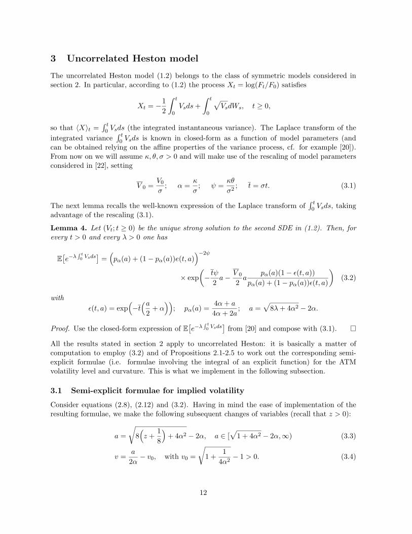
3 Uncorrelated Heston model

The uncorrelated Heston model (1.2) belongs to the class of symmetric models considered insection 2. In particular, according to (1.2) the process Xt = log(Ft/F0) satisfies

Xt = −12

∫ t

0Vsds+

∫ t

0

√VsdWs, t ≥ 0,

so that 〈X〉t =∫ t0 Vsds (the integrated instantaneous variance). The Laplace transform of the

integrated variance∫ t0 Vsds is known in closed-form as a function of model parameters (and

can be obtained relying on the affine properties of the variance process, cf. for example [20]).From now on we will assume κ, θ, σ > 0 and will make use of the rescaling of model parametersconsidered in [22], setting

V 0 =V0

σ; α =

κ

σ; ψ =

κθ

σ2; t = σt. (3.1)

The next lemma recalls the well-known expression of the Laplace transform of∫ t0 Vsds, taking

advantage of the rescaling (3.1).

Lemma 4. Let (Vt; t ≥ 0) be the unique strong solution to the second SDE in (1.2). Then, forevery t > 0 and every λ > 0 one has

E[e−λ

∫ t0 Vsds

]=(pα(a) + (1− pα(a))e(t, a)

)−2ψ

× exp(− tψ

2a− V 0

2a

pα(a)(1− ε(t, a))pα(a) + (1− pα(a))ε(t, a)

)(3.2)

withε(t, a) = exp

(−t(a

2+ α

)); pα(a) =

4α+ a

4α+ 2a; a =

√8λ+ 4α2 − 2α.

Proof. Use the closed-form expression of E[e−λ

∫ t0 Vsds

]from [20] and compose with (3.1).

All the results stated in section 2 apply to uncorrelated Heston: it is basically a matter ofcomputation to employ (3.2) and of Propositions 2.1-2.5 to work out the corresponding semi-explicit formulae (i.e. formulae involving the integral of an explicit function) for the ATMvolatility level and curvature. This is what we implement in the following subsection.

3.1 Semi-explicit formulae for implied volatility

Consider equations (2.8), (2.12) and (3.2). Having in mind the ease of implementation of theresulting formulae, we make the following subsequent changes of variables (recall that z > 0):

a =

√8(z +

18

)+ 4α2 − 2α, a ∈ [

√1 + 4α2 − 2α,∞) (3.3)

v =a

2α− v0, with v0 =

√1 +

14α2− 1 > 0. (3.4)

12

The substitution (3.3) comes into play naturally when considering (3.2), while (3.4) simplifiesthe dependence to the parameter α and shifts the integration back to (0,∞). After thesesubstitutions and the proper simplifications (remark that we have z = α2

2 v(v+ 2v0 + 2)), we get

E[e−(z+ 18)It ] = h(t, v), (3.5)

with

h(t, v) = P (t, v)−2ψ exp(−αψt(v0 + v)− αV 0(v0 + v)

P (t, v)− e(t, v))P (t, v)

);

P (t, v) = p(v) + (1− p(v))e(t, v);e(t, v) = exp(−αt(v0 + 1 + v));

p(v) =v0 + 2 + v

2(v0 + 1 + v); v0 =

√1 +

14α2− 1.

(3.6)

Equations (2.7) and (2.12) become respectively

P(Xt > 0) =1

2πα

∫ ∞0

g(v)h(t, v)dv

andpt(0) =

α

π

∫ ∞0

q(v)h(t, v)dv,

withg(v) =

v0 + 1 + v√v√

2(v0 + 1) + v (v0 + v)(v0 + 2 + v);

q(v) =v0 + 1 + v

√v√

2(v0 + 1) + v.

(3.7)

Since 12 < p(v) < 1 and 0 < e(t, v) < 1 for every v, t > 0, we observe that the function

h(t, v) is particularly well-behaved: in particular, v → h(t, v) is bounded for any value of t andexponentially decaying as v → ∞. On the other hand, the functions g and q diverge as 1√

vat

zero: to remove the singularity, we consider the additional change of variable

x =√v√

v + 1. (3.8)

The substitution (3.8) allows at the same time to remove the singularities at zero and to squeezethe integration over the bounded interval [0, 1]. So, we end up with the integral of boundedfunctions over the fixed interval [0, 1], a feature which is extremely convenient for numericalpurposes. Here are our final formulae.

Proposition 3.1 (ATM formulae). In the uncorrelated Heston model (1.2), for all t > 0 theATM implied volatility σ(t, 0) and the ATM density pt(0) of the log forward price Xt satisfy

σ(t, 0) = − 2√tN−1

( 1πα

∫ 1

0g(x)h(t, x)dx

), (3.9)

respectively

pt(0) =2απ

∫ 1

0q(x)h(t, x)dx (3.10)

13

with

g(x) =((v0 + 1)x2 + x2)x√

2(v0 + 1)x2 + x2 (v0x2 + x2)((v0 + 2)x2 + x2);

q(x) =(v0 + 1)x2 + x2

x3√

2(v0 + 1)x2 + x2;

h(t, x) = P (t, x)−2ψ exp(−αψtv0x

2 + x2

x2 − αV 0(v0x2 + x2)P (t, x)− e(t, x)

x2P (t, x)

);

P (t, x) = p(x) + (1− p(x))e(t, x); e(t, x) = exp(−αt(v0 + 1)x2 + x2

x2

);

p(x) =(v0 + 2)x2 + x2

2((v0 + 1)x2 + x2); x = (1− x); v0 =

√1 +

14α2− 1.

The ATM curvature of the implied variance is given by

∂2xσ(t, x)2|x=0 =

2t

(σ(t, 0)

√2πte

tσ2(t,0)8 pt(0)− 1

). (3.11)

Proof. Done above: the final claim is achieved performing the change of variable (3.8) in (3.6)-(3.7).

Remark 4. Actually, with the change of variable (3.8) we have introduced a singularity in thefunction q(x) as x tends to 1. But, unlike the singularity at zero, the divergence at x = 1 isstrongly dampened by the decreasing exponential in h(t, x). Hence, as happens for (3.9), theintegrand in (3.10) is smooth and bounded over [0, 1], too.

Prop 3.1 allows to compute the coefficients of the time-dependent SVI approximation given inProp 2.3. Recall that the extreme log-moneyness slope of implied variance is given by formula(1.1) in terms of the critical moment u∗. In the Heston model, the critical moment can becomputed as in Andersen and Piterbarg [1] or Keller-Ressel [13] (cf. also [22], Prop 11): theseauthors provide a closed-form formula for the explosion time t∗(u) = supt ≥ 0 : E[F ut ] < ∞,hence u∗(t) is obtained by numerical inversion of the equation t∗(u∗(t)) = t. For completenessof the presentation, we restate here this well known result (in the uncorrelated case), proposinga small variant of the statements in [1] and [13].

Proposition 3.2. Let β(t) = limx→±∞t σ(t,x)2

|x| , where σ(t, x) is the implied volatility in theuncorrelated Heston model. Then

β(t) = 4α(√

(1 + ω∗(t)2) +1

4α2−√

1 + ω∗(t)2)

(3.12)

where ω∗(t) is the unique solution in [ π2t ,πt ] of t∗(ω∗(t)) = ασ

2 t, with

t∗(ω) =2π − arccos

(1−ω2

1+ω2

)2ω

. (3.13)

This result can be proved without difficulty relying on affine principles as in [13] and performingan appropriate time rescaling of the involved Riccati equations. As it stands, the value of theasymptotic slopes given by (3.12) and (3.13) is not manifestly seen to coincide with Andersen and

14

Piterbarg’s and Keller-Ressel’s one, but it can be checked that the values of β(t) are actually thesame. The advantage of the formulation in Prop (3.2) is to make the function t∗ to be inversedindependent of model parameters: as a consequence, the values of the root ω∗ can be tabulatedonce for all, fastening the computations.

Let us come back to the SVI parameterisation. The functional form (2.17) we use to buildour approximation of implied volatility clearly belongs the original SVI class [9]. As pointedout in the Introduction, very recently Friz and other authors [8] have shown that at finitematurities (t < ∞) the Heston smile is not exactly described by the SVI parameterisation andthat an additional term should be added to SVI to account for the fine behaviour of the wings.Hence, to be consistent with Heston, we should take Friz et al.’s correction into account in ourapproximation: this would amount to an additional term of the form 2β1(t)β2(t)

√x. In our

framework, it is not obvious how to implement such a correction term for every log-moneynesswithout crushing the ATM structure: a term proportional to

√|x| would of course not have

the desired ATM convexity. Hence, even though the time-dependent SVI parameterisationwould benefit from the introduction of such a term in the far wings, the close to the moneystructure would be affected and we retain the parametric form (2.17) as it stands. This worksyet considerably well for reasonable ranges of model parameters, maturities and strikes (cf. theresults in section 5).

Here we restate Prop 2.3 in the framework of uncorrelated Heston.

Proposition 3.3. Let

a(t) = σ(t, 0)2 − β(t)2

t2∂2xσ(t, x)2|x=0

; b(t) =β(t)t

; γ(t) =β(t)

t∂2xσ(t, x)2|x=0

,

with σ(t, 0), ∂2xσ(t, x)2|x=0 and β(t) given by (3.9), (3.11) and (3.12) respectively. Then, the

parametric formσSV I(t, x)2 = a(t) + b(t)

√x2 + γ(t)2 (3.14)

has the same ATM level, ATM curvature and extreme log-moneyness slopes of the implied vari-ance under the uncorrelated Heston model (1.2) (cf. the “matching” properties of Proposition2.3).

The approximation (3.14) of the implied volatility in the uncorrelated Heston model is straight-forward to implement and computationally cheap: once the ATM implied volatility and cur-vature and the asymptotic slopes of the smile have been computed for a given maturity t, thecomputation of the whole smile (i.e. σ(t, x) for all the desired values of x) is instantaneous.The performances of this approximation for different strikes and maturities will be illustratedin section 5 by some numerical examples.

We close this section by making the statements of Proposition 2.4 specific to uncorrelatedHeston.

Proposition 3.4. In the uncorrelated Heston model (1.2), for all t > 0 and k ∈ R the density

15

pt(k) and the complementary cdf P(Xt > k) of the log forward price Xt are given by, respectively

pt(k) =2απ

∫ 1

0q(x)c(k, x)h(t, x)dx, (3.15)

P(Xt > k) =e−k/2

πα

∫ 1

0g(x)s(k, x)h(t, x)dx, (3.16)

wherec(k, x) = cos

(αkxx2 r(x)

);

s(k, x) = c(k, x)− 2αx

x2 r(x) sin(αkxx2 r(x)

);

r(x) =√

2(v0 + 1)x2 + x2;

x = (1− x); v0 =

√1 +

14α2− 1

and the functions g, h, q are the ones of Proposition 3.1.

Proof. Use (3.5) and the changes of variables (3.3)-(3.4)-(3.8) in (2.22) and (2.26).

As an immediate consequence (cf. Prop. 2.5), we obtain a formula for the price of a EuropeanCall option in the uncorrelated Heston model:

C(t, k) = F0P(Xt < log

F0

K

)−KP

(Xt > log

K

F0

)= F0

(1− 2

ek2

πα

∫ 1

0

((v0 + 1)x2 + x2)x cos(αkxx2 r(x)

)√2(v0 + 1)x2 + x2 (v0x2 + x2)((v0 + 2)x2 + x2)

h(t, x)dx),

(3.17)

where C(t, k) is a Call maturing at t and struck at K := F0ek and the function h(t, x) is given

in Prop. 3.1.

Remark 5. It seems to us that the formulation of Call options prices in (3.17) is new, sincesetting ρ = 0 in the classical solutions for Call prices based on extended Fourier transforms(cf. [12], [16] and many others) is not sufficient to get rid of the complex-valued functions.Proposition 3.4 provides indeed a fully “real” (in the algebraic sense) approach to option pricingin the Heston model.

4 An application to a skewed smile

Since market smiles are skewed, the uncorrelated Heston model (1.2) is quite unlikely to fit aset of market option prices. Nevertheless, the time-dependent SVI approximation (3.14) can bestraightforwardly applied to skewed smiles by considering a displaced model (cf. [21] and thesubsequent literature for displaced models). Let us give an example on the Heston model: let(Ft, t ≥ 0) be the forward price in a displaced Heston model,

dFt = (βFt + (1− β)F0)√VtdWt

dVt = κ(θ − Vt)dt+ σ√VtdZt,

(4.1)

16

where W,Z are independent Brownian motions and β ∈ [0, 1] is the displacement parameterintroducing the asymmetry in the model (β = 1 corresponding to zero displacement). As is wellknown, option pricing under (4.1) boils down to option pricing in the standard Heston model(1.2). Indeed, let

Ft = βFt + (1− β)F0, Vt = β2Vt, (4.2)

then the couple (F , V ) satisfies

dFt = Ft√VtdWt

dVt = κ(θ − Vt)dt+ σ√VtdZt

V0 = β2V0; θ = β2θ; σ = βσ,

(4.3)

hence (F , V ) is an uncorrelated Heston couple with “dislaced” parameters V0, θ, σ (F0 and κremain the same). The affine transformation (4.2) of the forward price and variance translatesinto the following mapping of the price CD of a Call in the displaced model onto the price in asymmetric model:

CD(t, x) := E[(Ft − F0ex)+]

=1β

E[(Ft − F0(1− β + βex)

)+],

(4.4)

hence the price of a Call on Ft equals 1/β times the price of a Call on Ft, the new log-moneynessbeing log(1− β + βex).We then simply approximate the implied volatility of the symmetric model (4.3) using the time-dependent SVI parameterisation (3.14). Denoting σSV I(t, x;V0, κ, θ, σ) the SVI approximationof the implied variance in the uncorrelated Heston model with parameters F0, V0, κ, θ, σ and(with obvious notation) CBS(t, x;σ) the price of a Black-Scholes Call, we have

CD(t, x) ≈ 1βCBS

(t, log(1− β + βex);σSV I

(t, log(1− β + βex);β2V0, κ, β

2θ, βσ)). (4.5)

Equation (4.5) gives a fast and economical approach to the pricing of Vanillas in the skeweddisplaced model (4.1).

5 Numerical Results

In this section we show the validity and accuracy of the representation formulae obtained insection 3 for the implied volatility in uncorrelated Heston. At all the time, our benchmark Calloption pricer is the usual semi-analytical pricer based on extended Fourier transforms (and thereference implied volatilities are obtained by numerical inversion of BS formula).

Table 1 compares the values of the implied volatility obtained by the standard pricing withthe ones obtained with formula (3.9), for a set of Heston parameters. The integration in (3.9)is performed using a fixed-tolerance Gaussian quadrature. The two series are perfectly in line,proving the validity of formula (3.9). Table 2 analyses the performances of the time-dependentSVI parametric form (3.14): we refer to this model as to the “Optimal SVI” in the sense ofthe matching of the ATM and far from the money structure as stated in Proposition 3.3. Only

17

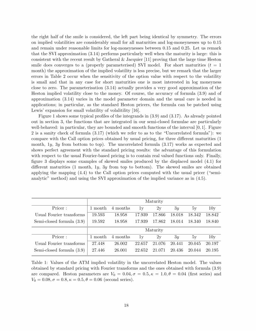
the right half of the smile is considered, the left part being identical by symmetry. The errorson implied volatilities are considerably small for all maturities and log-moneynesses up to 0.15and remain under reasonable limits for log-moneynesses between 0.15 and 0.25. Let us remarkthat the SVI approximation (3.14) performs particularly well when the maturity is large: this isconsistent with the recent result by Gatheral & Jacquier [11] proving that the large time Hestonsmile does converges to a (properly parameterised) SVI model. For short maturities (t = 1month) the approximation of the implied volatility is less precise, but we remark that the largererrors in Table 2 occur when the sensitivity of the option value with respect to the volatilityis small and that in any case for short maturities one is most interested in log moneynessclose to zero. The parameterisation (3.14) actually provides a very good approximation of theHeston implied volatility close to the money. Of course, the accuracy of formula (3.9) and ofapproximation (3.14) varies in the model parameter domain and the usual care is needed inapplications; in particular, as the standard Heston pricers, the formula can be patched usingLewis’ expansion for small volatility of volalitility [16].

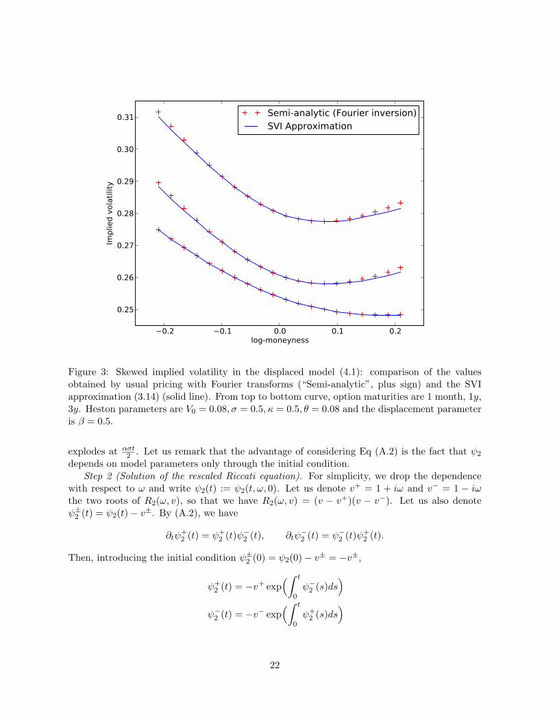
Figure 1 shows some typical profiles of the integrands in (3.9) and (3.17). As already pointedout in section 3, the functions that are integrated in our semi-closed formulae are particularlywell-behaved: in particular, they are bounded and smooth functions of the interval [0, 1]. Figure2 is a sanity check of formula (3.17) (which we refer to as to the “Uncorrelated formula”): wecompare with the Call option prices obtained by usual pricing, for three different maturities (1month, 1y, 3y from bottom to top). The uncorrelated formula (3.17) works as expected andshows perfect agreement with the standard pricing results: the advantage of this formulationwith respect to the usual Fourier-based pricing is to contain real valued functions only. Finally,figure 3 displays some examples of skewed smiles produced by the displaced model (4.1) fordifferent maturities (1 month, 1y, 3y from top to bottom). The skewed smiles are obtainedapplying the mapping (4.4) to the Call option prices computed with the usual pricer (“semi-analytic” method) and using the SVI approximation of the implied variance as in (4.5).

MaturityPricer : 1 month 4 months 1y 2y 3y 5y 10y

Usual Fourier transforms 19.593 18.958 17.939 17.866 18.018 18.342 18.842Semi-closed formula (3.9) 19.592 18.958 17.939 17.862 18.014 18.340 18.840

MaturityPricer : 1 month 4 months 1y 2y 3y 5y 10y

Usual Fourier transforms 27.448 26.002 22.657 21.076 20.441 20.045 20.197Semi-closed formula (3.9) 27.446 26.001 22.652 21.071 20.436 20.044 20.195

Table 1: Values of the ATM implied volatility in the uncorrelated Heston model. The valuesobtained by standard pricing with Fourier transforms and the ones obtained with formula (3.9)are compared. Heston parameters are V0 = 0.04, σ = 0.5, κ = 1.0, θ = 0.04 (first series) andV0 = 0.08, σ = 0.8, κ = 0.5, θ = 0.06 (second series).

18

t = 1 month log-moneynessModel: 0.0 0.025 0.05 0.10 0.15 0.20 0.25FT pricer 2.2556 1.2472 0.6256 0.1225 0.0185 0.0023 0.0002

19.59 19.68 19.92 20.71 21.68 22.70 23.72Optimal SVI 2.2556 1.2470 0.6245 0.1194 0.0167 0.0023 0.0002

19.59 19.68 19.91 20.60 21.41 22.24 23.06

t = 1 year log- moneynessModel: 0.0 0.025 0.05 0.10 0.15 0.20 0.25FT pricer 7.1461 6.0585 5.1162 3.6320 2.5830 1.8471 1.3286

17.94 17.98 18.12 18.59 19.26 20.04 20.87Optimal SVI 7.1461 6.0585 5.1152 3.6215 2.5519 1.7931 1.2570

17.94 17.98 18.11 18.56 19.16 19.84 20.54

t = 5 years log- moneynessModel: 0.0 0.025 0.05 0.10 0.15 0.20 0.25FT pricer 16.2466 15.2217 14.2421 12.4230 10.8006 9.3480 8.0792

18.34 18.35 18.37 18.43 18.56 18.70 18.89Optimal SVI 16.2466 15.2217 14.2421 12.430 10.7930 9.3585 8.0802

18.34 18.35 18.36 18.43 18.55 18.70 18.89

Table 2: Comparison of values of the implied volatility in the uncorrelated Heston model ob-tained by usual pricing with Fourier transforms (“FT pricer”) and with the time-dependent SVIapproximation (3.14) (“Optimal SVI”). Heston parameters are V0 = 0.04, σ = 0.5, κ = 1.0, θ =0.04. At each line, the first entry is the Call option price, the second entry the volatility.

Conclusion

We have obtained single-integral representation formulae for the ATM level and curvature of asymmetric smile generated by a continuous martingale. This result is based on the derivationof the corresponding representation formulae of the law (cumulative distribution and density)of the log forward price X in terms of the Laplace transform of the quadratic variation of X.These formulae take the form of the integral of an explicit real-valued function as soon as theLaplace transform in known in closed form, as e.g. in the Heston model. This result allows oneto build time-dependent SVI parameterisations which match the ATM and extreme moneynessstructure and are therefore optimal as SVI parameterisations of a symmetric smile. This time-dependent SVI model provides a very good and computationally cheap approximation of theimplied volatility in the uncorrelated Heston model, in particular close to the money. We haveaddressed how to apply this assembly to a skewed smile by considering a displaced model: asubject for future work is how to generalise this approach to the parameterisation of the smilesgenerated by a correlated stochastic volatility model.

19

Figure 1: Profiles of the function to be integrated in formula (3.9) to obtain the 1 monthATM implied volatility (left) and in formula (3.17) to obtain the price of a 1 month, log-moneyness= 0.2 Call option (right) in the uncorrelated Heston model.

Acknowledgments

We would like to thank Antoine Jacquier (TU Berlin and Zeliade Systems) and Jose da Fonseca(Auckland University of Technology, Ecole Superieure d’Ingenieurs Leonard de Vinci and ZeliadeSystems) for useful discussions on the subject of this work and for reading an earlier version ofthis manuscript, and Pierre Cohort (Zeliade Systems) for insights on displaced models.

A Proof of Proposition 3.2

The Heston model is an affine stochastic volatility model (ASVM), according to the definitionin [13]. In particular, we have

E[exp(uXt + vVt)

]= exp(φ(t, u, v) + uX0 + ψ(t, u, v)V0) (A.1)

for every (t, u, v) ∈ R+ ×R2 (allowing for the case where both sides of the identity are infinite).The functions φ and ψ satisfy the system of Riccati equations

∂tφ(t, u, v) = F (u, ψ(t, u, v)), φ(0, u, v) = 0∂tψ(t, u, v) = R(u, ψ(t, u, v)), ψ(0, u, v) = v

withF (u, v) = kθv

R(u, v) =12u(u− 1) +

σ2

2v2 − kv + ρσuv.

We aim here to compute the explosion time t∗(u) = supt ≥ 0 : E[exp(uXt)] < ∞, u > 1.Recalling that X0 = 0, by (A.1) we have E[exp(uXt)] = exp(φ(t, u, 0) + ψ(t, u, 0)V0). Sinceφ(t, u, v) = kθ

∫ t0 ψ(s, u, v)ds, it follows that t∗(u) is the explosion time of ψ(·, u, 0), that is

t∗(u) = supt ≥ 0 : ψ(t, u, 0) < ∞. Therefore we focus on the equation for ψ, in the uncorre-lated case ρ = 0.

20

Figure 2: A “sanity check” of formula (3.17) (the “Uncorrelated formula”) for Call option pricesin the uncorrelated Heston model. Comparison with the usual pricing with Fourier transformis shown. From bottom curve to top curve, option maturities are 1 month, 1y , 3y. Hestonparameters are V0 = 0.08, σ = 0.5, κ = 0.5, θ = 0.08.

Proof of Proposition 3.2. Step 1 (Rescaling of the Riccati equation). Recalling the parameterrescaling (3.1), we have

R(u,v

σ

)=

12u(u− 1) + v2 − αv =

12

(v − α)2 − 12(α2 − u(u− 1)

)Hence, defining

u(ω) :=12

+

√α2(1 + ω2) +

14, ω > 0; R2(ω, v) :=

2α2R(u(ω), α

v

σ

)we have R2(ω, v) = (v − 1)2 + ω2. It is easy to check that, for every ω > 0, the solution to theRiccati equation

∂tψ2(t, ω, v) = R2(ω, ψ2(t, ω, v)), ψ2(0, ω, v) =σ

αv (A.2)

is such thatψ(t, u(ω), v) =

α

σψ2

(ασt2, ω, v

)(A.3)

for all t. We will show (Step 3) that for u ≤ u(0), ψ(t, u, 0) is finite for all t. Hence it is sufficientto compute the explosion time of ψ2(·, ω, 0): by (A.3), ψ(·, u(ω), 0) explodes at t iff ψ2(·, ω, 0)

21

0.2 0.1 0.0 0.1 0.2log-moneyness

0.25

0.26

0.27

0.28

0.29

0.30

0.31Im

plie

d v

ola

tilit

ySemi-analytic (Fourier inversion)SVI Approximation

Figure 3: Skewed implied volatility in the displaced model (4.1): comparison of the valuesobtained by usual pricing with Fourier transforms (“Semi-analytic”, plus sign) and the SVIapproximation (3.14) (solid line). From top to bottom curve, option maturities are 1 month, 1y,3y. Heston parameters are V0 = 0.08, σ = 0.5, κ = 0.5, θ = 0.08 and the displacement parameteris β = 0.5.

explodes at ασt2 . Let us remark that the advantage of considering Eq (A.2) is the fact that ψ2

depends on model parameters only through the initial condition.Step 2 (Solution of the rescaled Riccati equation). For simplicity, we drop the dependence

with respect to ω and write ψ2(t) := ψ2(t, ω, 0). Let us denote v+ = 1 + iω and v− = 1 − iωthe two roots of R2(ω, v), so that we have R2(ω, v) = (v − v+)(v − v−). Let us also denoteψ±2 (t) = ψ2(t)− v±. By (A.2), we have

∂tψ+2 (t) = ψ+

2 (t)ψ−2 (t), ∂tψ−2 (t) = ψ−2 (t)ψ+

2 (t).

Then, introducing the initial condition ψ±2 (0) = ψ2(0)− v± = −v±,

ψ+2 (t) = −v+ exp

(∫ t

0ψ−2 (s)ds

)ψ−2 (t) = −v− exp

(∫ t

0ψ+

2 (s)ds)

22

hence, taking ratios,ψ2(t)− v+

ψ2(t)− v−=ψ+

2 (t)ψ−2 (t)

=1 + iω

1− iωexp(2iωt).

It follows that ψ2(t) is finite valued until there is a t such that the lhs is worth 1, that is a tsuch that

exp(2iωt) =1− iω1 + iω

=1− ω2

1 + ω2− 2i

ω

1 + ω2. (A.4)

As ω ranges from 0 to ∞, the lhs of this expression turns counterclockwise on the unit circle,while the rhs fills the lower half unit circle clockwise, from right to left. Hence, the smaller twhich solves Eq. (A.4) is such that π < 2ωt < 2π and that cos(2ωt) = 1−ω2

1+ω2 , that is

t∗(ω) =2π − arccos

(1−ω2

1+ω2

)2ω

.

Recalling the time scaling (A.3), the critical exponent u∗(t) = infu > 0 : E[exp(uXt)] =∞ =infu > 0 : ψ(t, u, 0) = ∞ is given by u∗(t) = u(ω∗(t)), where ω∗(t) is the unique solution in[ π2t ,

πt ] of t∗(ω∗(t)) = ασ

2 t. Eq (3.12) now follows easily from the expression of u(ω) and fromLee’s moment formula (1.1).

Step 3. Let us come back to R(u, v) : the two roots of v 7→ R(u, v) are

v± =α±

√α2 − u(u− 1)σ

.

If 0 < u < u(0) = 12 +

√α2 + 1

4 , then α2 − u(u − 1) > 0 and v+ and v− are both real with0 < v− < v+. Then, the same arguments as in Step 2 yield

ψ(t, u, 0)− v+

ψ(t, u, 0)− v−=v+

v−exp((v+ − v−)t)

and it is easy to see that this entails that ψ(t, u, 0) is finite for all t. Finally, if u = u(0), then v+ =v− = α/σ and R(u(0), v) = σ2

2

(v − α

σ

)2. The equation ∂tψ(t, u(0), 0) = σ2

2

(ψ(t, u(0), 0) − α

σ

)2can be solved by separation of variables, giving

ψ(t, u(0), 0) =α2t

ασt+ 2

hence ψ(t, u(0), 0) is finite for all t, too.

References

[1] L. Andersen and V. Piterbarg. Moment explosion in stochastic volatility models. Financeand Stochastics, 11:29–50, 2007.

[2] S. Benaim and P. Friz. Regular variation and smile asymptotics. Mathematical Finance,(1):1–12, 2006.

[3] H. Berestycki, J. Busca, and I. Florent. Computing the implied volatility in stochasticvolatility models. Communications on Pure and Applied Mathematics, pages 1352–1373,2004.

23

[4] P. Carr and R. Lee. Put-call symmetry : Extensions and applications. To appear inMathematical Finance.

[5] D. Dufresne. The integrated square-root process. Research Paper no. 90, Centre for Actu-arial Studies, University of Melbourne, 2001.

[6] M. Forde and A. Jacquier. Small-time asymptotics for implied volatility under the hestonmodel. Forthcoming in International Journal of Theoretical and Applied Finance, 2009.

[7] M. Forde, A. Jacquier, and A. Mijatovic. Asymptotic formulae for implied volatility underthe heston model. Forthcoming in Proceedings of the Royal Society A, 2009.

[8] P. Friz, S. Gerhold, A. Gulisashvili, and S. Sturm. On refined volatility smile expansion inthe heston model. Working paper, 2010.

[9] J. Gatheral. A parsimonious arbitrage-free implied volatility parameterization with appli-cation to the valuation of volatility derivatives. Presentation at Global Derivatives & RiskManagement, Madrid, May 2004.

[10] J. Gatheral. The volatility surface: A practitioner’s guide. Wiley Finance, 2006.

[11] J. Gatheral and A. Jacquier. Convergence of heston to SVI. Working Paper Series, Availableat SSRN: http://ssrn.com/abstract=1555251, 2010.

[12] S. Heston. A closed-form solution for options with stochastic volatility with applications tobond and currency options. The Review of Financial Studies, 6(2):327–343, 1993.

[13] M. Keller-Ressel. Moment explosions and long-term behavior of affine stochastic volatilitymodels. Forthcoming in Mathematical Finance, 2009.

[14] N. N. Lebedev. Special functions and their applications. Dover, New York, 1972.

[15] R. W. Lee. The moment formula for implied volatility at extreme strikes. MathematicalFinance, 14, 2004.

[16] A. L. Lewis. Option valuation under stochastic volatility, with mathematica code. Financepress, 2005.

[17] A. Medvedev and O. Scaillet. A simple calibration procedure of stochastic volatility modelswith jumps by short term asymptotic. FAME Research Paper Series rp93, InternationalCenter for Financial Asset Management and Engineering, 2004.

[18] K. S. Miller and S. G. Samko. Completely monotonic functions. Integr. Transf. and Spec.Funct., (4):389–402, 2001.

[19] E. Renault and Nizar Touzi. Option hedging and implied volatilities in a stochastic volatilitymodel. Mathematical Finance, 6(3):279–302, 1996.

[20] D. Revuz and M. Yor. Continuous Martingales and Brownian motion, third edition.Springer, 1999.

[21] M. Rubinstein. Displaced diffusion option pricing. Journal of Finance, pages 125–144, 1983.

24

[22] Zeliade Systems. Heston 2009. Zeliade Systems White Paper, 2009. available online athttp://www.zeliade.com/whitepapers/zwp-0004.pdf.

[23] M. R. Tehranchi. Asymptotics of implied volatility far from maturity. Journal of AppliedProbability, 46(3):629–650, 2009.

[24] M. R. Tehranchi. Symmetric martingales and symmetric smiles. Stochastic Processes andTheir Applications, 119(10):3785–3797, 2009.

25