interest rate models’ implied volatility function ...thomasho.com/papers/joim2005353 final.pdf ·...

JOIM (2005) 1–34 Implied Volatility Function

Interest Rate Models’ Implied Volatility FunctionStochastic Movements

Thomas S. Y. Ho, Ph.D1∗, Blessing Mudavanhu, Ph.D2†

1 President, Thomas Ho Company Ltd, 55 Liberty Street, New York, NY 100052 Vice President, Merrill Lynch & Co., 4 World Financial Center, New York, NY

10080

Received Draft; revised 21 November, 2005

Abstract: This paper presents a one factor and a two factor arbitrage-free interest rate modelswith parsimonious implied volatility functions. The models are empirically tested on the entireswaption surface in three currencies (U. S. dollar, Euro and Japanese yen) over a five yearperiod. They are shown to be robust in explaining the swaption values, and the implied volatilityfunctions are shown to exhibit a three factor movement in all three currencies.

The results show that the observed swaption prices incorporate the market conditionalexpectations of the correlations of the key interest rates and the stochastic process of theyield curve, and the interest rate models should be calibrated to such market information toprovide accurate relative valuation. Further this paper describes a modeling approach that hasimportant implications on hedging interest rate derivatives dynamically taking the stochasticvolatility risks into account.c© To appear in Journal of Investment Management. All rights reserved.

Keywords: multi-factor arbitrage-free interest rate models, binomial lattice, interest ratederivatives, implied volatility function, vega risk, swaption, stochastic volatilities, volatilitysurface, key rate duration, key rate vega

1 Introduction

Arbitrage-free interest rate models such as Ho-Lee (1986, 2005), Heath, Jarrow and Mor-

ton (1992) HJM, Brace, Gatarek and Musiela (1997) BGM have broad applications in

securities valuation. In particular, they are used extensively to value interest rate con-

tingent claims such as derivatives and balance sheet items with embedded interest rate

∗ E-mail: [email protected]† E-mail: [email protected]

2 Ho and Mudavanhu / Implied Volatility Function (2005) 1–34

options. The models are also used to determine the key rate durations or PV 01 to specify

the dynamic hedging strategies in managing interest rate risks by measuring the interest

rate derivatives sensitivities to the key rates along the yield curve.

However, interest rate derivatives’ returns can be significantly affected by the changes in

the volatility, and that means the vega measure (the proportional increase in value to a

unit increase in volatility) is not negligible. Collin-Dufresne and Goldstein (2002) uses

interest rate straddles to provide empirical evidence of “unspanned stochastic volatility”

showing that interest rate derivatives cannot be dynamically hedged or replicated by

bonds (with no embedded options), because of the significant presence of the volatility

risk. Heidari and Wu (2003) uses the principal component analysis and shows that the

volatility surface of swaptions has three orthogonal movements, independent of the prin-

cipal movements of the yield curve . Other empirical studies of interest rate models have

shown that the implied volatilities are stochastic (Amin and Morton, De Jong, Driessen,

and Pelsser (2001)). Further Amin and Ng (1997) has shown that the implied volatilities

have informational content in predicting the future interest rate volatilities. Therefore,

vega measures are important to manage the volatility risk in hedging, risk reporting,

integrating market risks on the trading floor or on the enterprize level.

To date, there are significant challenges to determine the vega buckets for interest rate

derivatives. The first challenge is the computational intensity required in determining the

measurement. Pietersz and Pelsser (2003) uses the BGM model to determine the vega

buckets confining to swaptions on the anti-diagonal buckets (where the sum of expiry

and tenor is 31 years) of the swaption volatility surface and that process requires 1 to

5.8 million scenario paths. However, Heidari and Wu shows that the volatility risk is not

confined to the anti-diagonal buckets of the volatility surface. The entire surface gener-

ates the independent movements. Therefore, to extend the key rate duration measures

to the volatility surface poses a practical problem, and dynamically hedging an interest

rate derivative position remains intractable.

Another challenge is the use of interest rate models to determine the dynamic hedging.

To determine the vega measure, we require the interest rate model to be (1) accurate in

pricing the swaptions, (2) stable in the estimated parameters without overspecification,

and (3) computationally efficient. Despite the prevalent use of arbitrage-free interest rate

models, thus far, there is a lack of empirical evidence of an interest rate model that has

the above three attributes.

Most empirical studies to date are limited to test the models using short dated interest

rate derivatives or over a short sample period (Amin and Morton (1994), Mathis and

Bierwag (1999), Gupta and Subrahmanyam (2005), Flesaker (1993)). And these tests

assume non-stochastic term structure of volatilities. As a result, scant empirical studies

have provided insights into the current practical use of the arbitrage-free interest rate

models in valuing the long dated swaptions and measuring the vega, though some recent

papers begin to deal with these issues.

Ho and Mudavanhu / Implied Volatility Function (2005) 1–34 3

Han (2005) and Jarrow, Li and Zhao (2004) extend the string model and the HJM model

respectively to incorporate the unspanned stochastic volatility. These approaches require

four stochastic factors for the yield curve movements and three stochastic factors for the

volatility risks, and over ten parameters have to be estimated. Extensive computation

may be required to compute the sensitivities of interest rate derivatives. Further, these

papers have not addressed the empirical issues raised above.

The purpose of this paper is to fill this void by providing a solution to manage the

volatility risk. We do so by using the generalized Ho-Lee model (2005). We first show

that the model has high explanatory power for the observed swaption prices across 1-

10 year expiry and 1-20 year tenor (the entire volatility surface), using a one factor and

two factor models with less than five parameters. Then we show that the volatility sur-

face movements can be represented by the movements of two volatility curves (“implied

volatility functions”) analogous to the yield curve in the volatility space. We can reduce

the movement of the volatility surface to the movements of two curves. As a result, we

can determine the vega at the key points on these curves, the “key rate vega”. Since the

generalized Ho-Lee model provides a computationally efficient method to value a broad

range of interest rate derivatives, this paper provides a methodology to manage the risk

of interest rate derivatives by combining the use of key rate durations and key rate vegas.

This paper contributes to the extensive literature in interest rate modeling in several ways.

First, this paper presents two interest rate models with parsimonious implied volatility

functions and empirically tested the models. We examine the one factor and the two

factor generalized Ho-Lee models on the a broad range of swaptions, which are central to

the derivatives market, over a five year period across three major currencies, U.S. dollar

(USD), Euro (EUR), and Japanese yen (JPY). This extension provides a validation of

the model for a key segment of the derivatives market in the major currencies. Second,

we empirically specify the stochastic movements of the implied volatility functions to

specify the principal movements of the volatility surface. As a result, this paper provides

the empirical implications of the use of arbitrage-free interest rate models in the capital

markets both in valuation and in managing the yield curve risks.

Our main results can be summarized as follows. We show that (1) the time series of resid-

ual mean square errors of both the one factor and the two factor models are generally

less than two Black volatility points, within a typical bid-ask spread for the at-the-money

swaptions in USD and EUR, and generally less than three Black volatility points in JPY;

(2) the two factor model provides a slightly higher explanatory power, and both the one

and the two factor models have the least valuation errors in the USD market; (3) the

implied volatility function has three orthogonal movements for each currency, together

explaining over 95% of the implied volatility function movements; (4) the model parame-

ters are stable, providing an effective key rate vega measure for risk management.

Our results can also provide some insights into previous empirical literature. De Jong,


Driessen, and Pelsser (2001) investigates the BGM model by studying the swaption re-

turns. Our result shows that such tests have to control the vega risk, which contributes

significantly to the swaption returns. Our approach is similar to that of Amin and Morton

in calibrating the implied volatility function. We differ in our sample data and interest

rate models. We analyze the swaptions and not the short dated Euro futures options, as in

their test, and we investigate the stochastic movements of the implied volatility functions,

beyond specifying the functions. Longstaff, Santa-Clara and Schwartz (2001) calibrates

a four factor string model to 34 at-the-money swaptions, as opposed to calibrating the

volatility surface of 91 at-the-money swaptions in this paper, with their errors ranging

between 2% to 16%. Han (2005) extends the string model to incorporate an additional

three stochastic volatility factors with lower errors. The difference in the performance of

these models in fitting the swaption prices can be explained by the alternative approaches

in modeling that we take in this paper.

The generalized Ho-Lee model differs from these models by calibrating (1) the correla-

tions of the key rates, implying the yield curve movements from the swaption prices, and

(2) the interest rate stochastic distribution (switching between two processes used in this

paper), inferring a mix of “lognormal” and “normal” distributions also from the market

prices. This approach is entirely consistent with the basic premise of the arbitrage-free

rate movement models. This way, the model incorporates the continually changing views

of the market in the yield curve movements, in the rates correlation and the distribu-

tion. By way of contrast, both the string model and the market model use historical

correlations and pre-specified interest rate distributions. Such an approach would not

incorporate the conditional expectation of the yield curve movements, for example, the

anticipation of the change of yield curve steepening and the behavior of the tails of the

distribution, to the valuation model.

The paper proceeds as follows. Section 2 describes the generalized Ho-Lee model, which

provides the theoretical framework to specify the implied volatility function. Section 3

describes the empirical estimation method and the data. Section 4 presents the empiri-

cal results of the estimated errors and the specification of the implied volatility function

movements for the one factor model of the three currencies. Section 5 compares the

results of the two factor models to those of the one factor models. Section 6 describes

the method in hedging the stochastic volatility risks and introduces the key rate vega

measure. Section 7 contains the conclusions.

2 Theoretical Model

Our approach is consistent with current practice of valuing interest rate contingent claims

and the management of interest rate risks. Brace Gatarek and Musiela (1997) and

Jamshidian (1997) proposed the market models, which are arbitrage-free models that

fit not only the spot yield curve but also the caps/floors (LIBOR model) or a sample

of swaptions (Swaption Model). In essence, these models fit the model volatilities to


the benchmark options over the entire range of tenors instead of calibrating the implied

volatility function to a sample of options as in Amin and Morton. The growing inter-

ests in such market models in capital markets underscore two important aspects of the

arbitrage-free models assumed in practice.

First, the market benchmark options, for example, the caps/floors and at-the-money

swaptions (“volatility surface”), are liquid. To many practitioners, the volatility surface

is as important as the term structure of interest rates in valuing the interest rate deriv-

atives. The entire market volatility surface, and not a volatility number, is often used

to value derivatives, and therefore the arbitrage-free interest rate model must necessar-

ily be consistent with these benchmark options. Second, the volatility function of the

arbitrage-free model is not perceived to be constant. It is implicitly assumed that “prices

in stochastic volatility models are of similar form to those in a constant volatility model,

with volatility terms in the latter replaced by their conditional expected levels in the sto-

chastic volatility environment. [Hull and White (1987)]” Thus, using a constant volatility

model with market-implied volatility parameters achieves nearly the same effect.

2.1 Implied Volatility Function

Arbitrage-free interest rate models can be uniquely specified by the term structure of

volatilities, a function of time and states. The parameters of the function can be implied

from the observed prices of the traded options. Such a function is called the “implied

volatility function”, which can be interpreted as the market perceived interest rate un-

certainties into the future.

Specifically, interest rate models may be specified as follows:

dr(t) = α(t, r)dt + σ(t, r(t))dW (t) (1)

where r is the instantaneous interest rate, α(t, r) is the drift term that fits the model

to the observed spot curve, σ(t, r(t)) is the implied volatility function and dW is the

standard Brownian motion.

Some examples of the implied volatility function are:

• Absolute (Ho-Lee): σ(·) = σ0

• Square Root (Cox, Ingersoll, Ross): σ(·) = σ0r(t)1/2

• Proportional (Courtadon): σ(·) = σ0r(t)

• Linear Absolute: σ(·) = σ0 + σ1(t)

• Exponential (Vasicek): σ(·) = σ0 exp(−ct), where c is a constant.


The generalized Ho-Lee model that we study empirically in this paper has the implied

volatility function is given by

σ(a, b, c, d, R) = ((a + bt) exp(−ct) + d) min[r(t), R] (2)

The parameters (a, b, c, d) can be interpreted as follows. When interest rates are below the

threshold rate R, (a+d) and d are the instantaneous and long term short rate volatilities

respectively. c is the exponential decay rate which is directly related to the extent of

the mean reversion process of interest rates, ensuring the long term volatility to be lower

than the short term volatility (and this parameter is also used in the Vasecek model),

and b determines the size of the hump of the volatility curve.

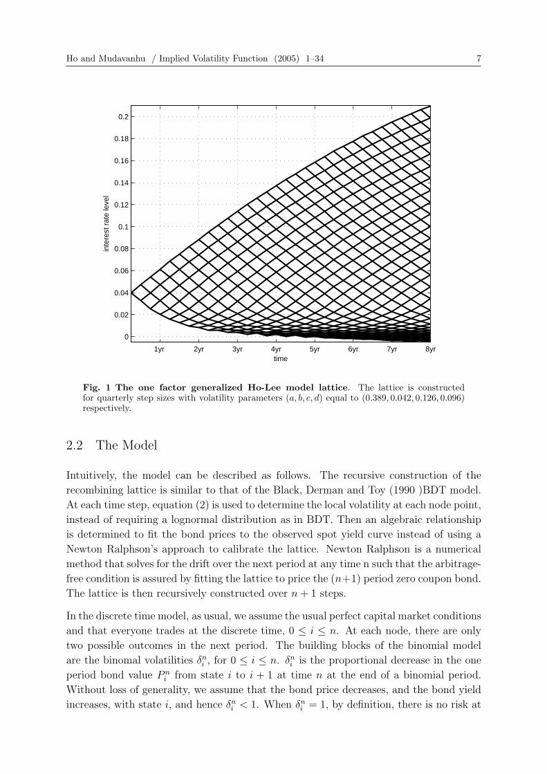
The threshold rate R, enables the model to switch from a normal model to a lognormal

model when interest rates are low. This switch of regime would determine a lower bound

for and disallow explosive rise of interest rates. If R is an arbitrarily large constant,

then the model is a lognormal model. Conversely, if R is an arbitrarily small constant,

then the model is a normal model. Figure 1 below depicts the behavior of the one factor

generalized Ho-Lee model. The lattice shows that the interest rates rise linearly on the

top boundary (a normal model) and the rates fall proportionally on the bottom boundary

(a lognormal model). For the empirical test, we will fix the threshold rate. For clarity of

the exposition, and without loss of generality, we will refer to the function below as the

“implied volatility function” for the generalized Ho-Lee model. The level of the threshold

rate R only affects the distribution of interest rates and not the specific shape of the

implied volatility function. For this reason, keeping R constant does not affect the main

conclusions of the paper.

σ(a, b, c, d) = (a + bt) exp(−ct) + d (3)

The parsimonious specification of the implied volatility function, using only four para-

meters, avoids over specification of the model. In principle, any curve fitting methods

using multiple parameters can be used to perfectly fit the implied volatility function to

observed prices of the benchmark securities. See Lee and Choi (2005), which is akin to

that employed by the market models. However, the purpose of this paper is not to show

that the interest rate model can fit the spot curve and the volatility surface. The purpose

of this paper is to show that the model with few parameters can explain many observed

swaption prices over an extensive sample period. And for this reason, we are testing the

functional form of equation (3) empirically.

The parameters (a, b, c, d) can be interpreted as follows. When interest rates are below

the threshold rate, (a + d) and d are the instantaneous long term and short rate volatili-

ties, respectively. The constant c is the exponential decay rate which is directly related

to the extent of the mean reversion process, and b determines the size of the hump of the

volatility curve.


1yr 2yr 3yr 4yr 5yr 6yr 7yr 8yr

0

0.02

0.04

0.06

0.08

0.1

0.12

0.14

0.16

0.18

0.2

time

inte

rest

rat

e le

vel

Fig. 1 The one factor generalized Ho-Lee model lattice. The lattice is constructedfor quarterly step sizes with volatility parameters (a, b, c, d) equal to (0.389, 0.042, 0.126, 0.096)respectively.

2.2 The Model

Intuitively, the model can be described as follows. The recursive construction of the

recombining lattice is similar to that of the Black, Derman and Toy (1990 )BDT model.

At each time step, equation (2) is used to determine the local volatility at each node point,

instead of requiring a lognormal distribution as in BDT. Then an algebraic relationship

is determined to fit the bond prices to the observed spot yield curve instead of using a

Newton Ralphson’s approach to calibrate the lattice. Newton Ralphson is a numerical

method that solves for the drift over the next period at any time n such that the arbitrage-

free condition is assured by fitting the lattice to price the (n+1) period zero coupon bond.

The lattice is then recursively constructed over n + 1 steps.

In the discrete time model, as usual, we assume the usual perfect capital market conditions

and that everyone trades at the discrete time, 0 ≤ i ≤ n. At each node, there are only

two possible outcomes in the next period. The building blocks of the binomial model

are the binomal volatilities δni , for 0 ≤ i ≤ n. δn

i is the proportional decrease in the one

period bond value P ni from state i to i + 1 at time n at the end of a binomial period.

Without loss of generality, we assume that the bond price decreases, and the bond yield

increases, with state i, and hence δni < 1. When δn

i = 1, by definition, there is no risk at


the binomial node with respect to the upstate and downstate outcomes. More generally,

let δni (T ) denote the binomial volatility of a T term bond. Since cash, bond with zero

maturity, has no risk, by convention, we have

δni (0) = 1 (4)

The implied volatility function equation (3) in the binomial lattice framework is re-written

as

σ(n) = (a + b · n∆t) exp(−c · n∆t) + d (5)

where ∆t is the interval of one period, for 0 ≤ i ≤ n. For example, if one period (the

step size of the lattice) is one month, then ∆t is 1/12.

The binomal volatilities δni are defined by the volatility function σ(n) in the equation (5),

as follows‡:δni = exp(−2σ(n) min[− log P n

i , R∆t]∆t1/2) (6)

R is the threshold rate, as explained in the previous section. Equation (6) translates the

volatility measure as the standard deviation of the proportional change in rates to the

proportional change in prices.

By the construction of the arbitrage-free rate model, the binomial volatilities have to

satisfy the recursive equation

δni (T ) = δn

i δn+1i (T + 1)

[1 + δn+1

i+1 (T − 1)

1 + δn+1i (T − 1)

](7)

The binomial volatilities in equation (7) specifies the one period bond pricing model at

node (n, i):

P ni =

P (n + 1)

P (n)

n∏

k=1

(1 + δk−10 (n− k))

(1 + δk−10 (n− k + 1))

i−1∏j=0

δn−1j (8)

This system of recursive equations (4)–(8) defines the binomial model of the generalized

one factor Ho-Lee model.

The two factor Ho-Lee model can be specified analogously, below

P ni,j(T ) =

P (n + 1)

P (n)×

n∏

k=1

(1 + δk−10,1 (n− k))

(1 + δk−10,1 (n− k + 1))

× (1 + δk−10,2 (n− k))

(1 + δk−10,2 (n− k + 1))

×i−1∏

k=0

δn−1k,1 (T )×

j−1∏

k=0

δn−1k,2 (T ) (9)

‡ Since this is a discrete time model, the interest rates can still become negative as a result ofthe discrete time approximation, even for some small volatilities when the rates are low. Equa-tion (6) cannot ensure that δn

i are always bounded by one. For implementation, we use δni =

exp(−2σ(n)max[min[− log Pni , R∆t]∆t1/2, ε]) for some small ε , say, 0.0001 or 1 basis point, effectively

switching the model to a normal model with an arbitrarily low volatility and determines a lower boundof the negative rates. See Ho and Lee (2005) for further extension of the model in controlling the extentof exhibiting negative rates of the model.


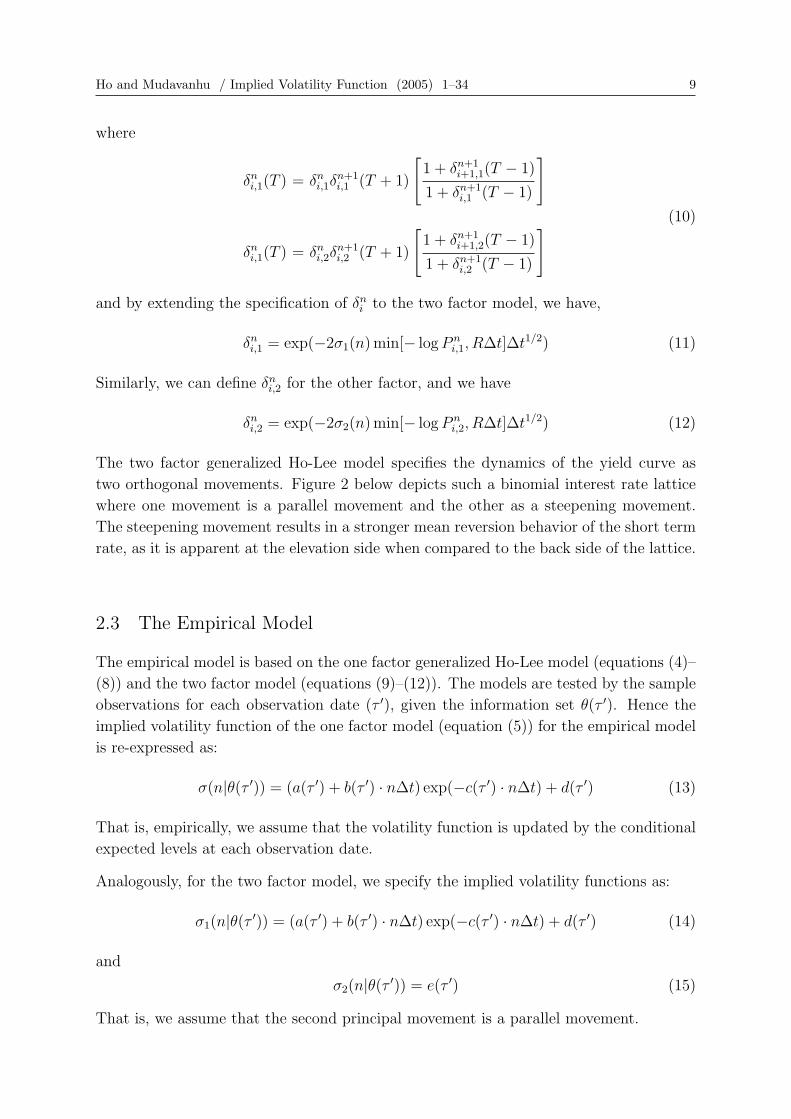
where

δni,1(T ) = δn

i,1δn+1i,1 (T + 1)

[1 + δn+1

i+1,1(T − 1)

1 + δn+1i,1 (T − 1)

]

(10)

δni,1(T ) = δn

i,2δn+1i,2 (T + 1)

[1 + δn+1

i+1,2(T − 1)

1 + δn+1i,2 (T − 1)

]

and by extending the specification of δni to the two factor model, we have,

δni,1 = exp(−2σ1(n) min[− log P n

i,1, R∆t]∆t1/2) (11)

Similarly, we can define δni,2 for the other factor, and we have

δni,2 = exp(−2σ2(n) min[− log P n

i,2, R∆t]∆t1/2) (12)

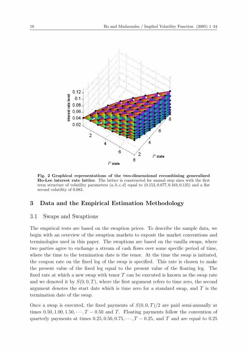
The two factor generalized Ho-Lee model specifies the dynamics of the yield curve as

two orthogonal movements. Figure 2 below depicts such a binomial interest rate lattice

where one movement is a parallel movement and the other as a steepening movement.

The steepening movement results in a stronger mean reversion behavior of the short term

rate, as it is apparent at the elevation side when compared to the back side of the lattice.

2.3 The Empirical Model

The empirical model is based on the one factor generalized Ho-Lee model (equations (4)–

(8)) and the two factor model (equations (9)–(12)). The models are tested by the sample

observations for each observation date (τ ′), given the information set θ(τ ′). Hence the

implied volatility function of the one factor model (equation (5)) for the empirical model

is re-expressed as:

σ(n|θ(τ ′)) = (a(τ ′) + b(τ ′) · n∆t) exp(−c(τ ′) · n∆t) + d(τ ′) (13)

That is, empirically, we assume that the volatility function is updated by the conditional

expected levels at each observation date.

Analogously, for the two factor model, we specify the implied volatility functions as:

σ1(n|θ(τ ′)) = (a(τ ′) + b(τ ′) · n∆t) exp(−c(τ ′) · n∆t) + d(τ ′) (14)

and

σ2(n|θ(τ ′)) = e(τ ′) (15)

That is, we assume that the second principal movement is a parallel movement.


Fig. 2 Graphical representations of the two-dimensional recombining generalizedHo-Lee interest rate lattice. The lattice is constructed for annual step sizes with the firstterm structure of volatility parameters (a, b, c, d) equal to (0.152, 0.077, 0.164, 0.125) and a flatsecond volatility of 0.083.

3 Data and the Empirical Estimation Methodology

3.1 Swaps and Swaptions

The empirical tests are based on the swaption prices. To describe the sample data, we

begin with an overview of the swaption markets to exposit the market conventions and

terminologies used in this paper. The swaptions are based on the vanilla swaps, where

two parties agree to exchange a stream of cash flows over some specific period of time,

where the time to the termination date is the tenor. At the time the swap is initiated,

the coupon rate on the fixed leg of the swap is specified. This rate is chosen to make

the present value of the fixed leg equal to the present value of the floating leg. The

fixed rate at which a new swap with tenor T can be executed is known as the swap rate

and we denoted it by S(0, 0, T ), where the first argument refers to time zero, the second

argument denotes the start date which is time zero for a standard swap, and T is the

termination date of the swap.

Once a swap is executed, the fixed payments of S(0, 0, T )/2 are paid semi-annually at

times 0.50, 1.00, 1.50, · · · , T − 0.50 and T . Floating payments follow the convention of

quarterly payments at times 0.25, 0.50, 0.75, · · · , T − 0.25, and T and are equal to 0.25


times the three-month LIBOR rate at the beginning of the quarter. A floating rate note

paying three-month LIBOR quarterly must worth par at each quarterly LIBOR reset

date. Since the initial value of the swap is zero, the initial value of the fixed leg must

also be worth par. The swap rates are available from a variety of sources, for standard

swap tenors such as 1, 2, 3, 4, 5, 7, 10, 12, 15, 20, 25 and 30 years, in real time.

We use vanilla European swaptions in this paper. The holder of the swaption has an

option to enter into a swap and receive (or pay) fixed payments. The holder of the option

has a right at time τ to enter into a swap with a remaining term T − τ , and receive (or

pay) the fixed annuity based on semi-annual compounding rate of c. This option is called

a τ into T − τ receivers (or payers) swaption, where τ is the time to expiration of the

option and T − τ is the tenor of the underlying swap.

The convention in the swaptions market is to quote prices in terms of their implied

volatilities relative to the Black (1976) model as applied to the forward swap rate. The

Black model implies that the value of a τ by T European payers swaption at time zero is

V (0, τ, T, c) =1

2A(0, τ, T )

[S(0, τ, T )Φ(d)− cΦ(d− σ

√τ)

](16)

where

d =ln(S(0, τ, T )/c) + σ2τ/2

σ√

τ(17)

where Φ(·) is the cumulative standard normal distribution function and σ is the volatility

of the forward swap rate, and A(0, τ, T ) is the present value of the annuity interest

payments. In the special case where the swaption is at the money the above valuation

formula reduces to

V (0, τ, T, S(0, τ, T )) = (D(0, τ)−D(0, T ))[2Φ(σ

√τ/2)− 1

](18)

Since this receiver swaption is at-the-money forward, the value of the corresponding

payers swaption is identical. Note that when an at-the-money swaption is quoted at an

implied volatility σ, the actual price that is paid by the purchaser of the swaption is given

by substituting σ into equation (18).

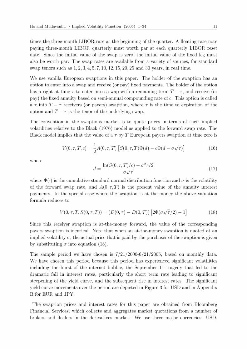
The sample period we have chosen is 7/21/2000-6/21/2005, based on monthly data.

We have chosen this period because this period has experienced significant volatilities

including the burst of the internet bubble, the September 11 tragedy that led to the

dramatic fall in interest rates, particularly the short term rate leading to significant

steepening of the yield curve, and the subsequent rise in interest rates. The significant

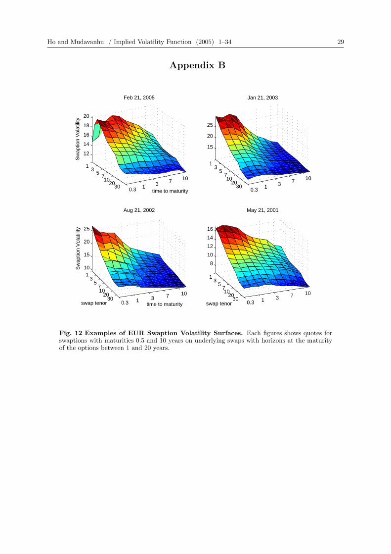
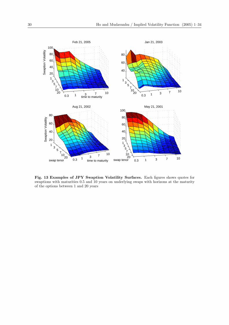
yield curve movements over the period are depicted in Figure 3 for USD and in Appendix

B for EUR and JPY.

The swaption prices and interest rates for this paper are obtained from Bloomberg

Financial Services, which collects and aggregates market quotations from a number of

brokers and dealers in the derivatives market. We use three major currencies: USD,


1m

6m

2yr

7yr

10yr

15yr

20yr

30yr

Jun05Jun04

Jun03Jun02

Jun01Jun00

1

2

3

4

5

6

7

term

US

D Z

ero

Rat

e (%

)

Fig. 3 Time Series of USD zero rates. The data set consists of monthly observations ofUSD zero curves with terms of one month to thirty years, for the period from June 2000 to June2005.

EUR and JPY, and the swaption are at-the-money options with expiration 1, 2, 3, 4,

5, 7,10 years and tenor 1, 2, 3, 4, 5, 6, 7, 8, 9,10, 12, 15, 20 years. Therefore there are

approximately 91 swaption observations for each month. There are 60 observation dates

in three currencies, in total 16,380 swaption observations. A summary description of the

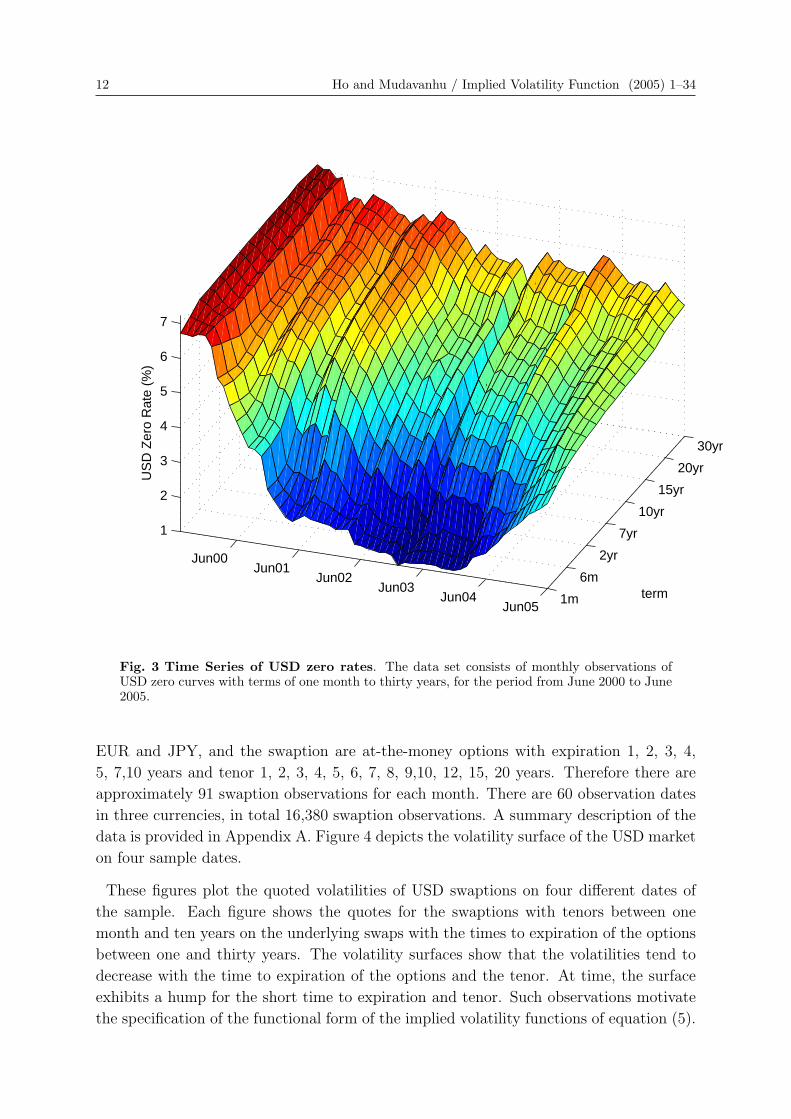
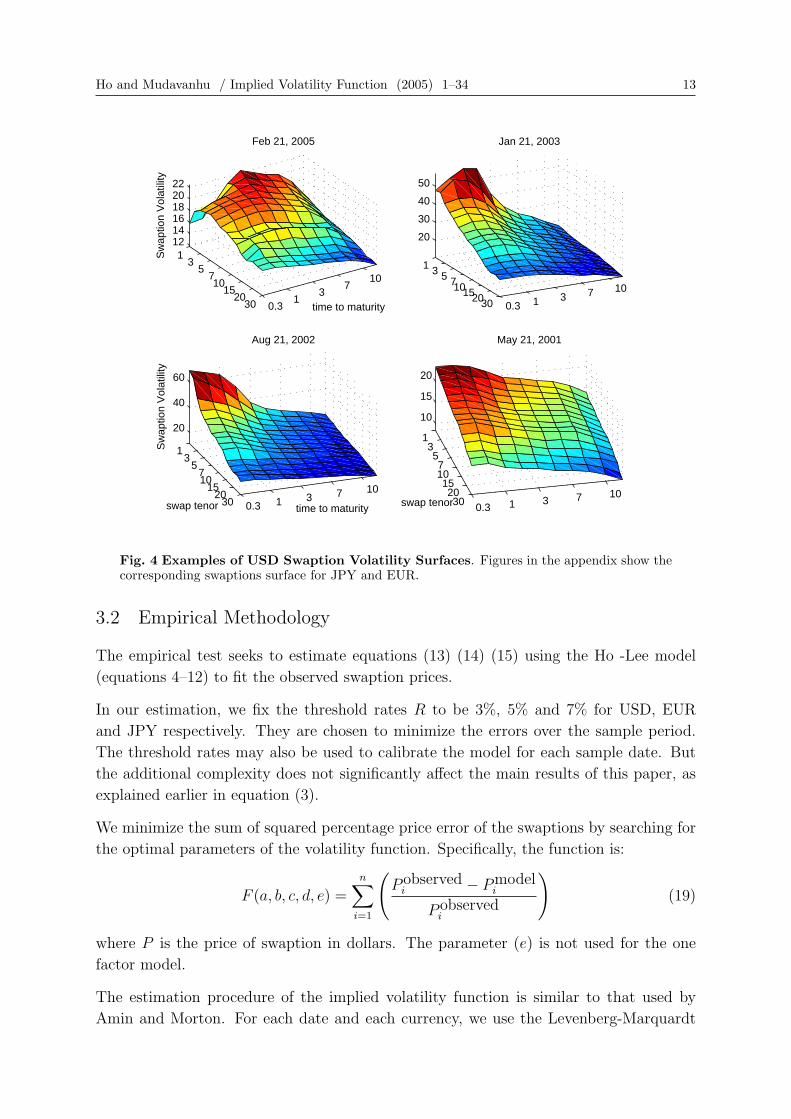
data is provided in Appendix A. Figure 4 depicts the volatility surface of the USD market

on four sample dates.

These figures plot the quoted volatilities of USD swaptions on four different dates of

the sample. Each figure shows the quotes for the swaptions with tenors between one

month and ten years on the underlying swaps with the times to expiration of the options

between one and thirty years. The volatility surfaces show that the volatilities tend to

decrease with the time to expiration of the options and the tenor. At time, the surface

exhibits a hump for the short time to expiration and tenor. Such observations motivate

the specification of the functional form of the implied volatility functions of equation (5).


13

5710

1520

30 0.31

37

10

121416182022

time to maturity

Feb 21, 2005

Sw

aptio

n V

olat

ility

1 3 5 710152030 0.3 1 3 7 10

20

30

40

50

Jan 21, 2003

13

5710

1520

30 0.3 1 3 7 10

20

40

60

time to maturity

Aug 21, 2002

swap tenor

Sw

aptio

n V

olat

ility

135710152030 0.3 1 3 7 10

10

15

20

May 21, 2001

swap tenor

Fig. 4 Examples of USD Swaption Volatility Surfaces. Figures in the appendix show thecorresponding swaptions surface for JPY and EUR.

3.2 Empirical Methodology

The empirical test seeks to estimate equations (13) (14) (15) using the Ho -Lee model

(equations 4–12) to fit the observed swaption prices.

In our estimation, we fix the threshold rates R to be 3%, 5% and 7% for USD, EUR

and JPY respectively. They are chosen to minimize the errors over the sample period.

The threshold rates may also be used to calibrate the model for each sample date. But

the additional complexity does not significantly affect the main results of this paper, as

explained earlier in equation (3).

We minimize the sum of squared percentage price error of the swaptions by searching for

the optimal parameters of the volatility function. Specifically, the function is:

F (a, b, c, d, e) =n∑

i=1

(Pobserved

i − Pmodeli

Pobservedi

)(19)

where P is the price of swaption in dollars. The parameter (e) is not used for the one

factor model.

The estimation procedure of the implied volatility function is similar to that used by

Amin and Morton. For each date and each currency, we use the Levenberg-Marquardt


algorithm, a non-linear estimation procedure, to minimize the objective function.

We use the percentage error instead of the volatility point error that Amin and Morton

uses because our measure enables us to appropriately compare across swaptions across

the currencies. Since we do not fit the volatility function to the observed swaption prices,

the goodness of the implied volatility function can be measured by the percentage errors

of the Black volatilities converted from the swaption prices. Specifically, we define the

error to be

Errori =

(νobserved

i − νmodeli

νobservedi

)(20)

for each swaption, at each date, for each currency, ν is the Black volatility measured in

percent.

4 One Factor Model Empirical Results: the Model Errors and

the Implied Volatility Function Movements

4.1 Analysis of the Model Errors

The result shows that the average percentage absolute errors over the sample period are

2.55, 3.36 and 5.74 for the USD, EUR and JPY respectively. These estimation errors are

within the bid-ask spreads in the market. To clarify the measure of errors, consider a

numerical illustration. Suppose a swaption value is quoted as 30 (Black) volatility points,

then 1% error as quoted in this paper is only 0.3 volatility point. This calibration is an

optimal search over only four parameters to fit 91 swaptions in most of the dates.

The results also show that the model can fit the USD market better than the EUR market,

which in turn is better than the JPY market. However, the coefficient of variations

(standard deviation/mean) are similar in magnitude, with the JPY value being lowest.

They are 0.34, 0.40 and 0.26 for USD, EUR and JPY respectively.

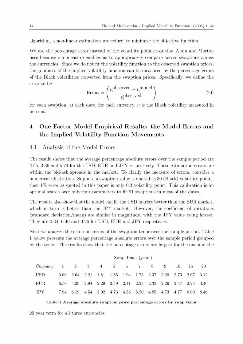
Next we analyze the errors in terms of the swaption tenor over the sample period. Table

1 below presents the average percentage absolute errors over the sample period grouped

by the tenor. The results show that the percentage errors are largest for the one and the

Swap Tenor (years)

Currency 1 2 3 4 5 6 7 8 9 10 15 20

USD 3.66 2.64 2.21 1.81 1.85 1.94 1.73 2.37 2.69 2.73 2.67 3.12

EUR 6.50 4.39 2.94 2.29 2.49 2.41 2.33 2.33 2.29 2.57 2.25 3.46

JPY 7.94 6.19 4.54 3.92 4.73 4.56 5.20 4.85 4.73 4.77 6.00 8.46

Table 1 Average absolute swaption price percentage errors by swap tenor

20 year term for all three currencies.


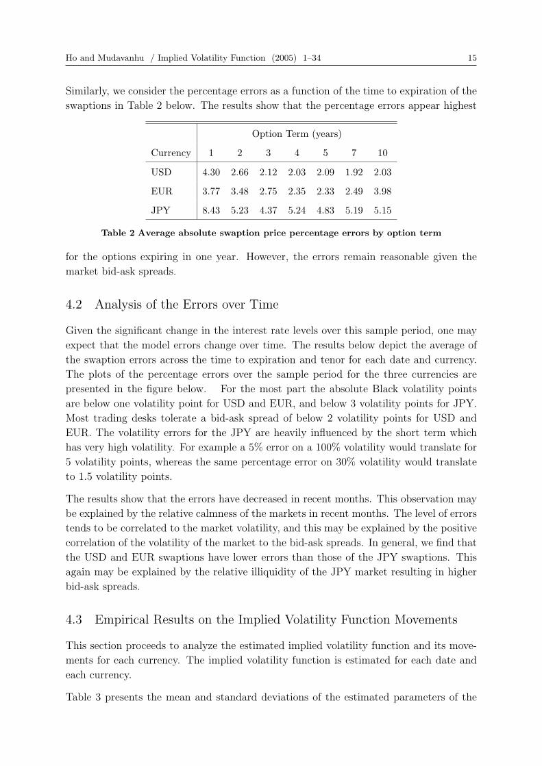
Similarly, we consider the percentage errors as a function of the time to expiration of the

swaptions in Table 2 below. The results show that the percentage errors appear highest

Option Term (years)

Currency 1 2 3 4 5 7 10

USD 4.30 2.66 2.12 2.03 2.09 1.92 2.03

EUR 3.77 3.48 2.75 2.35 2.33 2.49 3.98

JPY 8.43 5.23 4.37 5.24 4.83 5.19 5.15

Table 2 Average absolute swaption price percentage errors by option term

for the options expiring in one year. However, the errors remain reasonable given the

market bid-ask spreads.

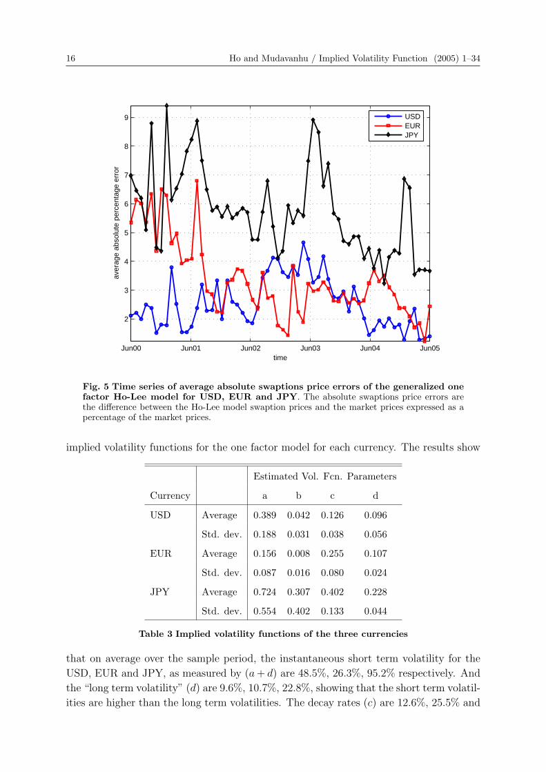
4.2 Analysis of the Errors over Time

Given the significant change in the interest rate levels over this sample period, one may

expect that the model errors change over time. The results below depict the average of

the swaption errors across the time to expiration and tenor for each date and currency.

The plots of the percentage errors over the sample period for the three currencies are

presented in the figure below. For the most part the absolute Black volatility points

are below one volatility point for USD and EUR, and below 3 volatility points for JPY.

Most trading desks tolerate a bid-ask spread of below 2 volatility points for USD and

EUR. The volatility errors for the JPY are heavily influenced by the short term which

has very high volatility. For example a 5% error on a 100% volatility would translate for

5 volatility points, whereas the same percentage error on 30% volatility would translate

to 1.5 volatility points.

The results show that the errors have decreased in recent months. This observation may

be explained by the relative calmness of the markets in recent months. The level of errors

tends to be correlated to the market volatility, and this may be explained by the positive

correlation of the volatility of the market to the bid-ask spreads. In general, we find that

the USD and EUR swaptions have lower errors than those of the JPY swaptions. This

again may be explained by the relative illiquidity of the JPY market resulting in higher

bid-ask spreads.

4.3 Empirical Results on the Implied Volatility Function Movements

This section proceeds to analyze the estimated implied volatility function and its move-

ments for each currency. The implied volatility function is estimated for each date and

each currency.

Table 3 presents the mean and standard deviations of the estimated parameters of the


Jun00 Jun01 Jun02 Jun03 Jun04 Jun05

2

3

4

5

6

7

8

9

time

aver

age

abso

lute

per

cent

age

erro

rUSDEURJPY

Fig. 5 Time series of average absolute swaptions price errors of the generalized onefactor Ho-Lee model for USD, EUR and JPY. The absolute swaptions price errors arethe difference between the Ho-Lee model swaption prices and the market prices expressed as apercentage of the market prices.

implied volatility functions for the one factor model for each currency. The results show

Estimated Vol. Fcn. Parameters

Currency a b c d

USD Average 0.389 0.042 0.126 0.096

Std. dev. 0.188 0.031 0.038 0.056

EUR Average 0.156 0.008 0.255 0.107

Std. dev. 0.087 0.016 0.080 0.024

JPY Average 0.724 0.307 0.402 0.228

Std. dev. 0.554 0.402 0.133 0.044

Table 3 Implied volatility functions of the three currencies

that on average over the sample period, the instantaneous short term volatility for the

USD, EUR and JPY, as measured by (a + d) are 48.5%, 26.3%, 95.2% respectively. And

the “long term volatility” (d) are 9.6%, 10.7%, 22.8%, showing that the short term volatil-

ities are higher than the long term volatilities. The decay rates (c) are 12.6%, 25.5% and



0.5

1

1.5

2

2.5

3

3.5

4

4.5

time

aver

age

abso

lute

vol

atili

ty p

oint

err

or (

%)

USDEURJPY

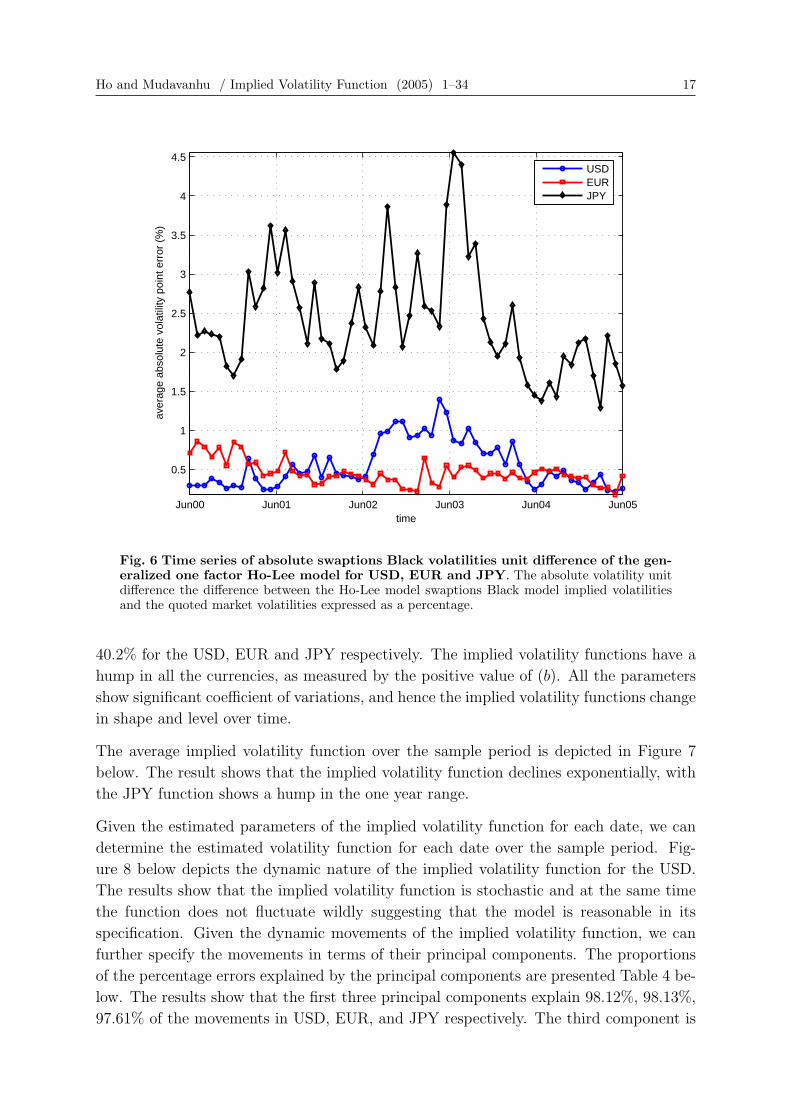
Fig. 6 Time series of absolute swaptions Black volatilities unit difference of the gen-eralized one factor Ho-Lee model for USD, EUR and JPY. The absolute volatility unitdifference the difference between the Ho-Lee model swaptions Black model implied volatilitiesand the quoted market volatilities expressed as a percentage.

40.2% for the USD, EUR and JPY respectively. The implied volatility functions have a

hump in all the currencies, as measured by the positive value of (b). All the parameters

show significant coefficient of variations, and hence the implied volatility functions change

in shape and level over time.

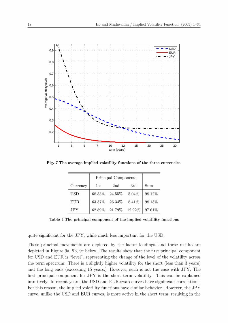
The average implied volatility function over the sample period is depicted in Figure 7

below. The result shows that the implied volatility function declines exponentially, with

the JPY function shows a hump in the one year range.

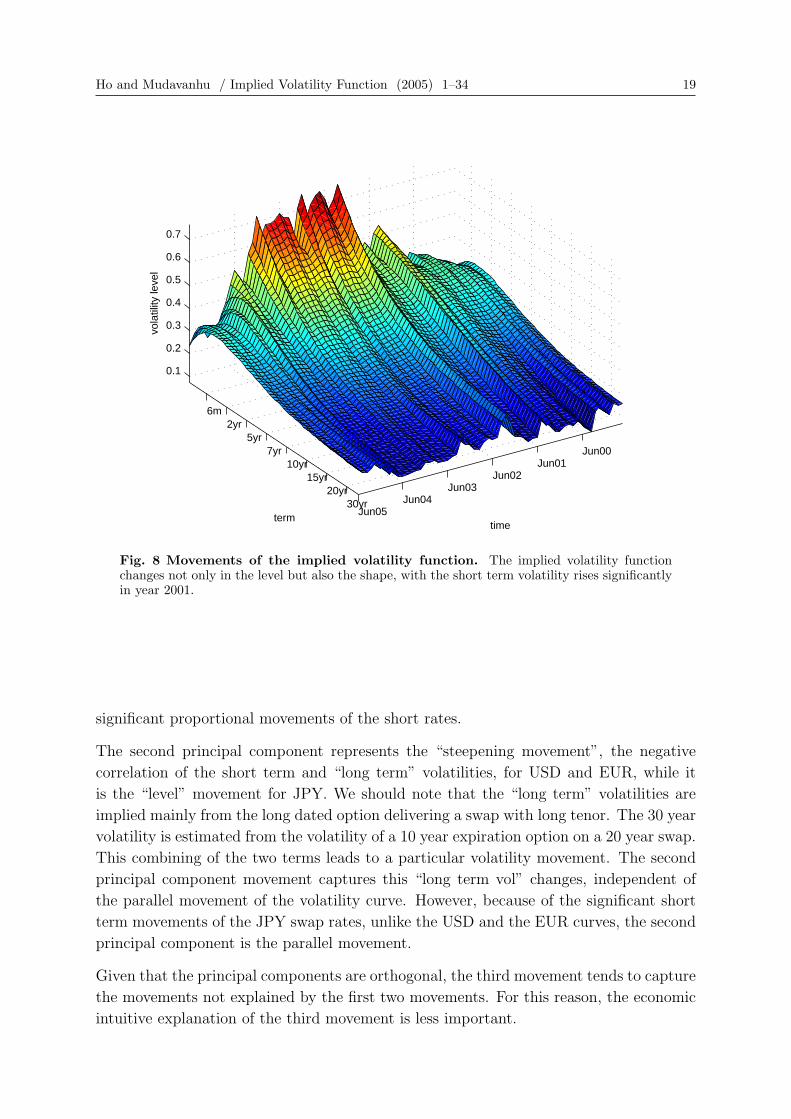
Given the estimated parameters of the implied volatility function for each date, we can

determine the estimated volatility function for each date over the sample period. Fig-

ure 8 below depicts the dynamic nature of the implied volatility function for the USD.

The results show that the implied volatility function is stochastic and at the same time

the function does not fluctuate wildly suggesting that the model is reasonable in its

specification. Given the dynamic movements of the implied volatility function, we can

further specify the movements in terms of their principal components. The proportions

of the percentage errors explained by the principal components are presented Table 4 be-

low. The results show that the first three principal components explain 98.12%, 98.13%,

97.61% of the movements in USD, EUR, and JPY respectively. The third component is


1 3 5 7 10 12 15 20 25 30

0.2

0.3

0.4

0.5

0.6

0.7

0.8

0.9

term (years)

aver

age

vola

tility

leve

lUSDEURJPY

Fig. 7 The average implied volatility functions of the three currencies.

Principal Components

Currency 1st 2nd 3rd Sum

USD 68.53% 24.55% 5.04% 98.12%

EUR 63.37% 26.34% 8.41% 98.13%

JPY 62.89% 21.79% 12.92% 97.61%

Table 4 The principal component of the implied volatility functions

quite significant for the JPY, while much less important for the USD.

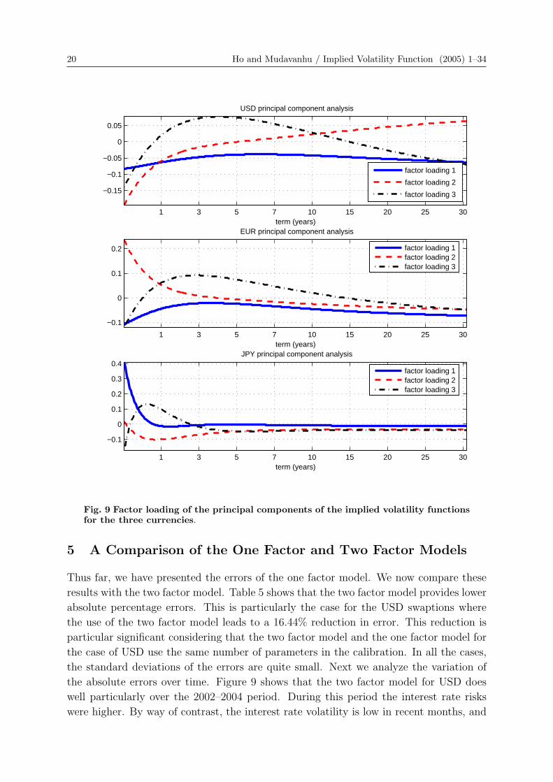
These principal movements are depicted by the factor loadings, and these results are

depicted in Figure 9a, 9b, 9c below. The results show that the first principal component

for USD and EUR is “level”, representing the change of the level of the volatility across

the term spectrum. There is a slightly higher volatility for the short (less than 3 years)

and the long ends (exceeding 15 years.) However, such is not the case with JPY. The

first principal component for JPY is the short term volatility. This can be explained

intuitively. In recent years, the USD and EUR swap curves have significant correlations.

For this reason, the implied volatility functions have similar behavior. However, the JPY

curve, unlike the USD and EUR curves, is more active in the short term, resulting in the


6m2yr

5yr7yr

10yr15yr

20yr30yr

Jun05Jun04

Jun03Jun02

Jun01Jun00

0.1

0.2

0.3

0.4

0.5

0.6

0.7

timeterm

vola

tility

leve

l

Fig. 8 Movements of the implied volatility function. The implied volatility functionchanges not only in the level but also the shape, with the short term volatility rises significantlyin year 2001.

significant proportional movements of the short rates.

The second principal component represents the “steepening movement”, the negative

correlation of the short term and “long term” volatilities, for USD and EUR, while it

is the “level” movement for JPY. We should note that the “long term” volatilities are

implied mainly from the long dated option delivering a swap with long tenor. The 30 year

volatility is estimated from the volatility of a 10 year expiration option on a 20 year swap.

This combining of the two terms leads to a particular volatility movement. The second

principal component movement captures this “long term vol” changes, independent of

the parallel movement of the volatility curve. However, because of the significant short

term movements of the JPY swap rates, unlike the USD and the EUR curves, the second

principal component is the parallel movement.

Given that the principal components are orthogonal, the third movement tends to capture

the movements not explained by the first two movements. For this reason, the economic

intuitive explanation of the third movement is less important.


1 3 5 7 10 15 20 25 30

−0.15

−0.1

−0.05

0

0.05

term (years)

USD principal component analysis

factor loading 1

factor loading 2

factor loading 3

1 3 5 7 10 15 20 25 30

−0.1

0

0.1

0.2

term (years)

EUR principal component analysis

factor loading 1factor loading 2factor loading 3

1 3 5 7 10 15 20 25 30

−0.1

0

0.1

0.2

0.3

0.4

term (years)

JPY principal component analysis

factor loading 1factor loading 2factor loading 3

Fig. 9 Factor loading of the principal components of the implied volatility functionsfor the three currencies.

5 A Comparison of the One Factor and Two Factor Models

Thus far, we have presented the errors of the one factor model. We now compare these

results with the two factor model. Table 5 shows that the two factor model provides lower

absolute percentage errors. This is particularly the case for the USD swaptions where

the use of the two factor model leads to a 16.44% reduction in error. This reduction is

particular significant considering that the two factor model and the one factor model for

the case of USD use the same number of parameters in the calibration. In all the cases,

the standard deviations of the errors are quite small. Next we analyze the variation of

the absolute errors over time. Figure 9 shows that the two factor model for USD does

well particularly over the 2002–2004 period. During this period the interest rate risks

were higher. By way of contrast, the interest rate volatility is low in recent months, and


Currency

USD EUR JPY

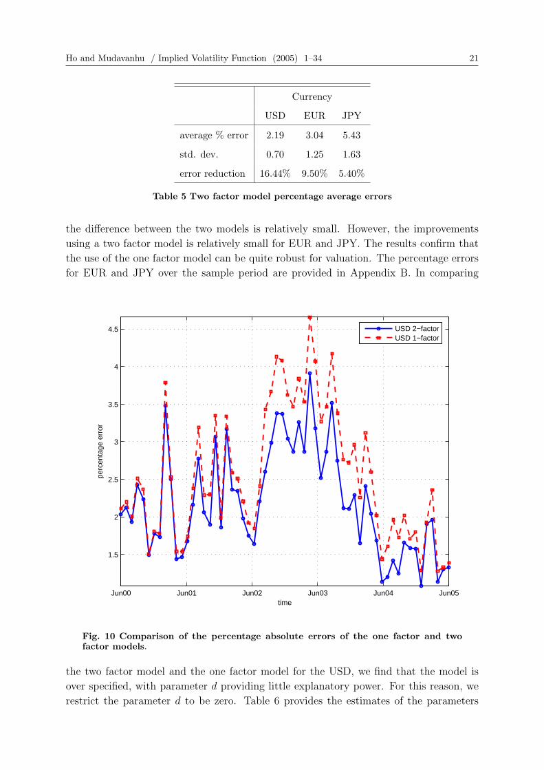
average % error 2.19 3.04 5.43

std. dev. 0.70 1.25 1.63

error reduction 16.44% 9.50% 5.40%

Table 5 Two factor model percentage average errors

the difference between the two models is relatively small. However, the improvements

using a two factor model is relatively small for EUR and JPY. The results confirm that

the use of the one factor model can be quite robust for valuation. The percentage errors

for EUR and JPY over the sample period are provided in Appendix B. In comparing


1.5

2

2.5

3

3.5

4

4.5

time

perc

enta

ge e

rror

USD 2−factorUSD 1−factor

Fig. 10 Comparison of the percentage absolute errors of the one factor and twofactor models.

the two factor model and the one factor model for the USD, we find that the model is

over specified, with parameter d providing little explanatory power. For this reason, we

restrict the parameter d to be zero. Table 6 provides the estimates of the parameters


of the implied volatility functions. In comparing the estimates of the parameters of the

Volatility 1 Volatility 2

Currency a b c d e

USD Average 0.401 0.050 0.128 0.046 0.099

Std. dev. 0.211 0.027 0.034 0.062 0.049

EUR Average 0.225 0.008 0.189 0.066 0.112

Std. dev. 0.096 0.011 0.039 0.048 0.014

JPY Average 0.739 0.399 0.430 0.159 0.122

Std. dev. 0.516 0.314 0.088 0.065 0.044

Table 6 The estimated parameters of the implied volatility functions

implied volatility function for the two factor and the one factor model, we see that the

implied volatility functions do not change significantly for USD and JPY. For the EUR,

the parameters a and b have changed but the qualitative behavior of the function remains

unchanged.

Following the analysis on the one factor model, we now proceed to analyze the dynamics of

the implied volatility function using the principal components of the movements. Consider

the results in Table 7. By introducing a second stochastic factor, the second principal

component becomes more significant in all the currencies, providing explanatory power of

more than 26% in all cases. Meanwhile, the first principal component remains significantly

dominant, exceeding 50% for all the currencies. The dynamic movements of the implied

Principal Components

Currency 1st 2nd 3rd Sum

USD 59.35% 32.56% 5.94% 97.86%

EUR 62.19% 26.7% 9.67% 98.56%

JPY 50.15% 27.55% 14.05% 91.75%

Table 7 Explanatory power of the principal components

volatility functions of the two factor model for USD are depicted below. The results show

that the volatility functions are quite dynamic, exhibiting higher volatility in the short

term.

This result is confirmed by estimating the factor loading of the principal components.

Figure 10 shows that the variation in the short term is captured by the first principal

components. We have described the results for the USD swaptions so far. However, these

observations also apply to the EUR and JPY swaptions, whose results are provided in

Appendix C.


1 3 5 7 10 15 20 25 30

−0.15

−0.1

−0.05

0

0.05

term (years)

factor loading 1

factor loading 2

factor loading 3

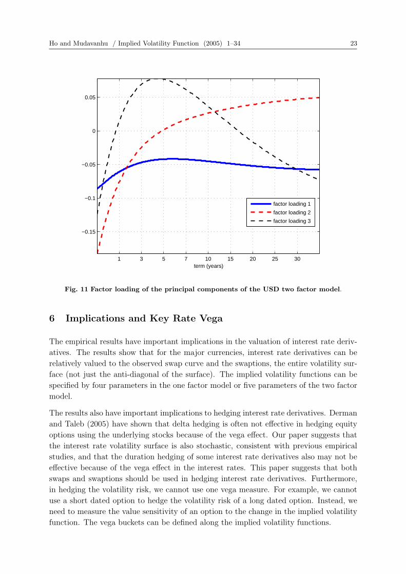
Fig. 11 Factor loading of the principal components of the USD two factor model.

6 Implications and Key Rate Vega

The empirical results have important implications in the valuation of interest rate deriv-

atives. The results show that for the major currencies, interest rate derivatives can be

relatively valued to the observed swap curve and the swaptions, the entire volatility sur-

face (not just the anti-diagonal of the surface). The implied volatility functions can be

specified by four parameters in the one factor model or five parameters of the two factor

model.

The results also have important implications to hedging interest rate derivatives. Derman

and Taleb (2005) have shown that delta hedging is often not effective in hedging equity

options using the underlying stocks because of the vega effect. Our paper suggests that

the interest rate volatility surface is also stochastic, consistent with previous empirical

studies, and that the duration hedging of some interest rate derivatives also may not be

effective because of the vega effect in the interest rates. This paper suggests that both

swaps and swaptions should be used in hedging interest rate derivatives. Furthermore,

in hedging the volatility risk, we cannot use one vega measure. For example, we cannot

use a short dated option to hedge the volatility risk of a long dated option. Instead, we

need to measure the value sensitivity of an option to the change in the implied volatility

function. The vega buckets can be defined along the implied volatility functions.


The construction of these changes is analogous to the construction of the changes on

the yield curve to determine the key rate durations. These value sensitivities are called

“key rate vegas”. The result shows that in hedging an interest rate option, we should

match the option to a portfolio of swaps and swaptions, such that the sets of both key

rate durations and key rate vegas are matched. The effectiveness of the key rate vegas

largely depends on the ability of the interest rate model in fitting the volatility surface,

something that the interest rate models presented can do. And thus the effectiveness of

the hedge should improve with the use of swaptions and swaps in matching the key rate

durations and key rate vegas. However, it is beyond the scope of this paper to present

the key rate vega measures in more details.

Key rate durations are widely used in managing interest rate risks. In managing an in-

terest rate derivative position with significant vega risks, this paper proposes to extend

the use of key rate durations to include key rate vegas, based on the implied volatility

functions. This approach is entirely consistent with the arbitrage-free interest rate mod-

eling approach. It does not seek to determine the “equilibrium model” as the unspanned

stochastic volatility models seek to do by using historical estimates of the correlation of

the interest rates. While the conditional expectations of the movements of the yield curve

and the volatility surface continually change over time, the hedging does not have to be

updated frequently, as demonstrated by the use of the key rate durations. Key rate vegas

enable us to measure the “unspanned risks”, and in this sense, the use of the implied

volatility function to determine the key rate vegas is a natural extension of the concept

of key rate durations.

7 Conclusions

This paper uses monthly data of swaptions in three major currencies to study the ro-

bustness of the generalized Ho and Lee models, their implied volatility functions and

movements. The empirical results show that the implied volatility functions are stochas-

tic and they can be used to define key rate vega to manage the volatility risk of interest

rate derivatives.

Specifically, we show that the implied volatility function exhibits movements with three

significant components. This result shows that the use of durations to implement dy-

namic hedging of derivatives or the use of short term options to hedge the vega of the

long dated options may not be effective. A more effective hedging approach would employ

also the swaptions that would match all the principal movements of the implied volatility

function, as well as the yield curve movements.

Acknowledgments

We would like to thank Yoon Seok Choi, Sang Bin Lee and Sanjay Nawalkha for their

comments and discussions. We are responsible for the remaining errors.


References

[1] Amin, Kaushik I and A. J. Morton, “Implied volatility functions in Arbitrage-freeterm structure models”, Journal of Financial economics, Vol. 35 (1994), pp. 141–180

[2] Amin, Kaushik I and Victor K. Ng, “Inferring Future Volatility from the Information inImplied Volatility in Eurodollar Options: A New Approach”, The Review of FinancialStudies, Vol. 10 (2) (summer 1997), pp. 333–367

[3] Bali, Turan G., “Modeling the Stochastic Behavior of Short-term Interest Rates:Pricing Implications for Discount Bonds”, Journal of Banking and Finance, 2003

[4] Black, Fischer, Emmanual Derman, William Toy, “A One Factor Model of InterestRates and its Applications to Treasury Bond Options”, Financial Analysts Journal,Vol. 46 (1990), 33–39

[5] Brace, A., D. Gatarek, and M. Musiela, “The Market Model of Interest RateDynamics”, Mathematical Finance, Vol. 7 (1997), pp. 127–155

[6] Buhler, Wolfgang, Marliese Uhrig-Homburg, Ulrich Walter, Thomas Weber, “AnEmpirical Comparison of Forward-Rate and Spot-rate Models for Valuing Interestrate options”, Journal of Finance, Vol. 54 (1) (February 1999), pp. 269–305

[7] Chapman, David and Neil Pearson, “Recent Advances in Estimating Term-StructureModels”, Financial Analysts Journal, July/Aug 2001, pp. 77

[8] Chan, K.C., G. Andrew Karolyi, Francis A. Longstaff, Anthony Sanders, “AnEmpirical Comparison of Alternative Models of the Short-Term Interest Rate”,Journal of Finance, Vol 47 (3), Papers and proceedings of the fifty-second annualmeeting of the American Finance Association, 1992, pp. 1209–1227

[9] Collin-Dufresne, Pierre and Robert Goldstein, “Do Bond Spans the Fixed IncomeMarkets? Theory and Evidence for Unspannned Stochastic Volatility”, Journal ofFinance, Vol LVII, No 4, August 2002

[10] Courtadon, G., “The pricing of options on Default-free Bonds”, Journal of FinancialQuantitative Analysis, Vol. 17 (1982), pp. 75–100

[11] Cox, J., J. Ingersoll, and S. Ross, “A Theory of the Term Structure of Interest Rates”,Econometrica, Vol. 53 (1985), pp. 385–407

[12] De Jong, Frank, Joost Driessen, and Antoon Pelsser, “Libor Market Models VersusSwap Market Models for Pricing Interest Rate Derivatives: an Empirical Analysis”,European Finance, Review 5 (2001), pp. 201–237

[13] Derman, E., and N. N. Taleb, “The Illusions of Dynamic Replication”, QuantitativeFinance, Vol. 5 (4) (2005), pp.323-326

[14] Flesaker, Bjorn, “Test the HJM/ HL Model of Interest Rate Contingent ClaimsPricing”, Journal of Quantitative Analysis, (1993), pp. 483–495

[15] Gupta, Anurag and Marti Subrahmanyam, “Pricing and Hedging interest rateoptions: evidence from cap-floor markets”, Journal of Banking and Finance, Vol.29 (2005), pp. 701–733

[16] Han, Bing, “Stochastic Volatilities and Correlations of Bond Yields”, Working Paper,Ohio State University, 2005

[17] Heidari, Massoud and Liuren Wu, “Are Interest Rate Derivatives Spanned by theTerm Structure of Interest Rates?”, Journal of Fixed Income, June 2003


[18] Ho, Thomas S. Y., “Key Rate Duration: a Measure of Interest Rate Risks Exposure”,Journal of Fixed Income Vol. 2 (2) (1992), pp. 29–44

[19] Ho, Thomas S. Y., and Sang Bin Lee, “Term Structure Movements and Pricing ofInterest Rate Contingent Claims”, Journal of Finance, Vol. 41 (1986), pp. 1011–1029

[20] Ho, Thomas S. Y., and Sang Bin Lee, The Oxford Guide to Financial Modeling,Oxford University Press (2004)

[21] Ho, Thomas S. Y., and Sang Bin Lee, “A Multi-Factor Binomial Interest Rate Modelwith State-Time-Dependent Volatilities”, THC Research Paper (2005)

[22] Ho, Thomas S. Y., Sang Bin Lee, and Yoon Seok Choi, “Practical Considerations inManaging the Risk of Variable Annuities”, THC Research Paper (2005)

[23] Ho, Thomas S. Y., and B. Mudavanhu, “Decomposing and Managing MultivariateRisks: The Case of Variable Annuities”, Journal of Investment Management, Vol. 3(4) (2005), pp.68-86.

[24] Hull, J. and A. White, “The Pricing of Options on Assets with StochasticVolatilities”, Journal of Finance, Vol. 42 (1987), pp. 281–300

[25] Jamshidian, Farshid, “LIBOR and Swap Market Models and Measures”, Finance andStochastics, Vol. 1 (1997), pp. 293–330

[26] Jarrow, Robert, Haitao Li, and Feng Zhao, “Interest Caps Smile Too! But Can theLIBOR Market Model Capture It?”, Working Paper, Cornell University, 2004

[27] Lee, Sang Bin and Yoon Seok Choi, “Generalized Ho-Lee Model as a Market Model:A Technical Note”, THC Research Paper (2005)

[28] Longstaff, F. A., P. Santa-Clara, and E. S. Schwartz, “The Relative Valuation ofCaps and Swaptions: Theory and Practical Evidence”, Journal of Finance, Vol. 56(6) (2001), pp. 2067–2110.

[29] Mathis lll, Roswell and Gerald Bierwag, “Pricing Eurodollar Futures Options withthe Ho and Lee and Black Derman and Toy model: an Empirical Comparison”, Journalof Financial Management, 1999

[30] Milevsky, Moshe. A., and S. D. Promislow, “Mortality Derivatives and the Optionto Annuitise”, Insurance: Mathematics and Economics, Vol. 29 (2001), pp. 299–318

[31] Pelsser, Antoon, “Pricing and Hedging Guaranteed Annuity Options via StaticOption Replication”, Insurance: Mathematics and Economics, Vol. 33 (2003), pp.283–296

[32] Pietersz, Raoul and Antoon Pelsser, “Risk-Managing Bermudan Swaptions in aLIBOR Model”, Journal of Derivatives, Vol. 11 (3) (2003), pp. 51–62

[33] Vasecek, O., “An equilibrium characterization of the term structure”, Journal ofFinancial Economics, Vol. 5 (1977), pp. 177–188


Appendix A

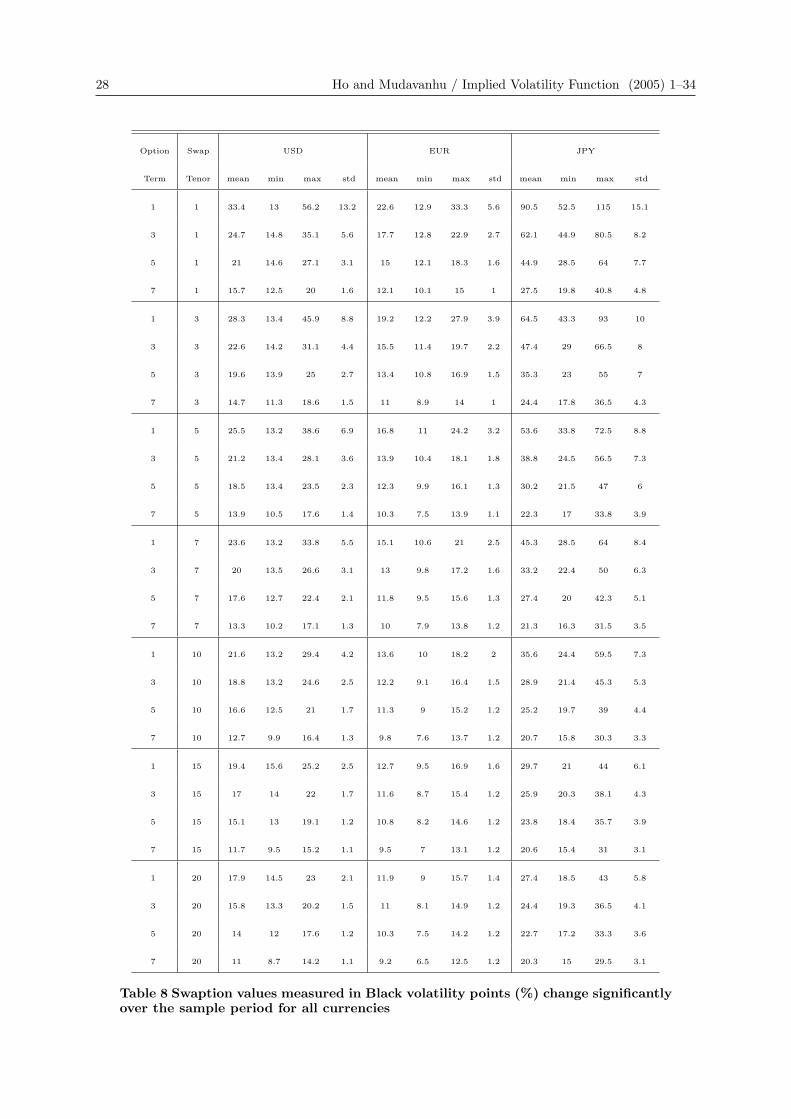
In the table below, we present the summary statistics (mean, minimum, maximum and

standard deviation) for at-the-money European swaption volatilities used for our empir-

ical study. The data consists of 60 monthly observations from July 21, 2000 to June 21,

2005 of mid-market implied Black model volatilities.


Option Swap USD EUR JPY

Term Tenor mean min max std mean min max std mean min max std

1 1 33.4 13 56.2 13.2 22.6 12.9 33.3 5.6 90.5 52.5 115 15.1

3 1 24.7 14.8 35.1 5.6 17.7 12.8 22.9 2.7 62.1 44.9 80.5 8.2

5 1 21 14.6 27.1 3.1 15 12.1 18.3 1.6 44.9 28.5 64 7.7

7 1 15.7 12.5 20 1.6 12.1 10.1 15 1 27.5 19.8 40.8 4.8

1 3 28.3 13.4 45.9 8.8 19.2 12.2 27.9 3.9 64.5 43.3 93 10

3 3 22.6 14.2 31.1 4.4 15.5 11.4 19.7 2.2 47.4 29 66.5 8

5 3 19.6 13.9 25 2.7 13.4 10.8 16.9 1.5 35.3 23 55 7

7 3 14.7 11.3 18.6 1.5 11 8.9 14 1 24.4 17.8 36.5 4.3

1 5 25.5 13.2 38.6 6.9 16.8 11 24.2 3.2 53.6 33.8 72.5 8.8

3 5 21.2 13.4 28.1 3.6 13.9 10.4 18.1 1.8 38.8 24.5 56.5 7.3

5 5 18.5 13.4 23.5 2.3 12.3 9.9 16.1 1.3 30.2 21.5 47 6

7 5 13.9 10.5 17.6 1.4 10.3 7.5 13.9 1.1 22.3 17 33.8 3.9

1 7 23.6 13.2 33.8 5.5 15.1 10.6 21 2.5 45.3 28.5 64 8.4

3 7 20 13.5 26.6 3.1 13 9.8 17.2 1.6 33.2 22.4 50 6.3

5 7 17.6 12.7 22.4 2.1 11.8 9.5 15.6 1.3 27.4 20 42.3 5.1

7 7 13.3 10.2 17.1 1.3 10 7.9 13.8 1.2 21.3 16.3 31.5 3.5

1 10 21.6 13.2 29.4 4.2 13.6 10 18.2 2 35.6 24.4 59.5 7.3

3 10 18.8 13.2 24.6 2.5 12.2 9.1 16.4 1.5 28.9 21.4 45.3 5.3

5 10 16.6 12.5 21 1.7 11.3 9 15.2 1.2 25.2 19.7 39 4.4

7 10 12.7 9.9 16.4 1.3 9.8 7.6 13.7 1.2 20.7 15.8 30.3 3.3

1 15 19.4 15.6 25.2 2.5 12.7 9.5 16.9 1.6 29.7 21 44 6.1

3 15 17 14 22 1.7 11.6 8.7 15.4 1.2 25.9 20.3 38.1 4.3

5 15 15.1 13 19.1 1.2 10.8 8.2 14.6 1.2 23.8 18.4 35.7 3.9

7 15 11.7 9.5 15.2 1.1 9.5 7 13.1 1.2 20.6 15.4 31 3.1

1 20 17.9 14.5 23 2.1 11.9 9 15.7 1.4 27.4 18.5 43 5.8

3 20 15.8 13.3 20.2 1.5 11 8.1 14.9 1.2 24.4 19.3 36.5 4.1

5 20 14 12 17.6 1.2 10.3 7.5 14.2 1.2 22.7 17.2 33.3 3.6

7 20 11 8.7 14.2 1.1 9.2 6.5 12.5 1.2 20.3 15 29.5 3.1

Table 8 Swaption values measured in Black volatility points (%) change significantlyover the sample period for all currencies


Appendix B

13

5710

2030 0.3 1 3 7 10

12

14

16

18

20

time to maturity

Feb 21, 2005

Sw

aptio

n V

olat

ility

13

5710

2030

0.3 1 3 7 10

15

20

25

Jan 21, 2003

13

5710

2030

0.3 1 3 7 10

10

15

20

25

time to maturity

Aug 21, 2002

swap tenor

Sw

aptio

n V

olat

ility

13

5710

2030

0.3 1 3 7 10

8

10

12

14

16

May 21, 2001

swap tenor

Fig. 12 Examples of EUR Swaption Volatility Surfaces. Each figures shows quotes forswaptions with maturities 0.5 and 10 years on underlying swaps with horizons at the maturityof the options between 1 and 20 years.


13571020

0.3 1 3 7 10

20

40

60

80

100

Feb 21, 2005

time to maturity

Sw

aptio

n V

olat

ility

13

5710

200.3 1 3 7 10

40

60

80

Jan 21, 2003

13

5710

200.3 1 3 7 10

20

40

60

80

time to maturity

Aug 21, 2002

swap tenor

Sw

aptio

n V

olat

ility

13571020

0.3 1 3 7 10

20

40

60

80

100May 21, 2001

swap tenor

Fig. 13 Examples of JPY Swaption Volatility Surfaces. Each figures shows quotes forswaptions with maturities 0.5 and 10 years on underlying swaps with horizons at the maturityof the options between 1 and 20 years


1m 6m 2yr 7yr 10yr 15yr 20yr 30yr

Jun05Jun04

Jun03Jun02

Jun01Jun00

2

2.5

3

3.5

4

4.5

5

5.5

6

term

EU

R Z

ero

Rat

e (%

)

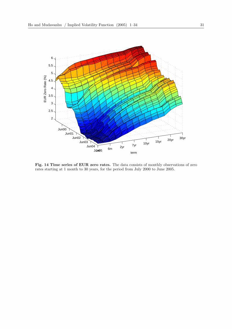
Fig. 14 Time series of EUR zero rates. The data consists of monthly observations of zerorates starting at 1 month to 30 years, for the period from July 2000 to June 2005.


1m6m

2yr7yr

10yr15yr

20yr30yr

Jun05

Jun04

Jun03

Jun02

Jun01

Jun00

0.5

1

1.5

2

2.5

term

JPY

Zer

o R

ate

(%)

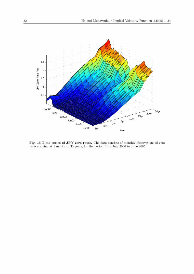
Fig. 15 Time series of JPY zero rates. The data consists of monthly observations of zerorates starting at 1 month to 30 years, for the period from July 2000 to June 2005.


Appendix C

6m 2yr 5yr 7yr 10yr 15yr 20yr 30yr

Jun05Jun04Jun03Jun02

Jun01Jun00

0.2

0.4

0.6

term

USD factor 1

vol.

leve

l

6m 2yr 5yr 7yr 10yr 15yr 20yr 30yr

Jun05Jun04Jun03Jun02

Jun01Jun000

0.1

0.2

term

USD factor 2

vol.

leve

l

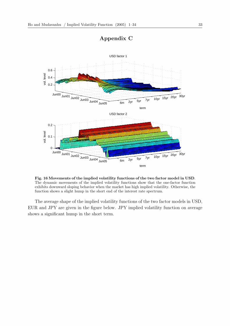
Fig. 16 Movements of the implied volatility functions of the two factor model in USD.The dynamic movements of the implied volatility functions show that the one-factor functionexhibits downward sloping behavior when the market has high implied volatility. Otherwise, thefunction shows a slight hump in the short end of the interest rate spectrum.

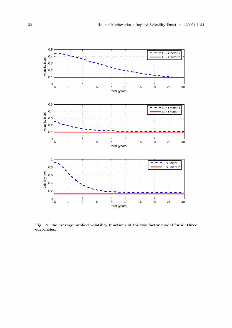
The average shape of the implied volatility functions of the two factor models in USD,

EUR and JPY are given in the figure below. JPY implied volatility function on average

shows a significant hump in the short term.


0.5 1 3 5 7 10 15 20 25 300

0.1

0.2

0.3

0.4

0.5

term (years)

vola

tility

leve

l

USD factor 1USD factor 2

0.5 1 3 5 7 10 15 20 25 300

0.1

0.2

0.3

0.4

0.5

term (years)

vola

tility

leve

l

EUR factor 1EUR factor 2

0.5 1 3 5 7 10 15 20 25 300

0.2

0.4

0.6

0.8

1

term (years)

vola

tility

leve

l

JPY factor 1JPY factor 2

Fig. 17 The average implied volatility functions of the two factor model for all threecurrencies.

interest rate models’ implied volatility function ...thomasho.com/papers/joim2005353 final.pdf ·...

Documents