the student t distribution - statpower notes/tdistribution.pdf · introduction student’s t...

IntroductionStudent’s t Distribution

Relationship to the One-Sample tRelationship to the t Test for Two Independent Samples

Relationship to the Correlated Sample tDistribution of the Generalized t Statistic

The Student t Distribution

James H. Steiger

Department of Psychology and Human DevelopmentVanderbilt University

James H. Steiger The Student t Distribution




The Student t Distribution1 Introduction

2 Student’s t Distribution

Basic Facts about Student’s t

3 Relationship to the One-Sample t

Distribution of the Test Statistic

The General Approach to Power Calculation

Power Calculation for the 1-Sample t

Sample Size Calculation for the 1-Sample t


4 Relationship to the t Test for Two Independent Samples

Distribution of the Test Statistic



5 Relationship to the Correlated Sample t

Distribution of the Correlated Sample t Statistic

6 Distribution of the Generalized t Statistic





Introduction

In this module, we review some properties of Student’s tdistribution.We shall then relate these properties to the null andnon-null distribution of some classic test statistics:

1 The 1-Sample Student’s t-test for a single mean.2 The 2-Sample independent sample t-test for comparing two

means.3 The 2-Sample “correlated sample” t-test for comparing two

means with correlated or repeated-measures data.4 The k-sample independent t-test for linear combinations of

means.

We then discuss power and sample size calculations usingthe developed facts.






Student’s t Distribution

In a preceding module, we discussed the classic z-statisticfor testing a single mean when the population variance issomehow known.Student’s t-distribution was developed in response to thereality that, unfortunately, σ2 is not known in the vastmajority of situations.Although substitution of a consistent sample-basedestimate of σ2 (such as s2, the familiar sample variance)will yield a statistic that is still asymptotically normal, thestatistic will no longer have an exact normal distributioneven when the population distribution is normal.The question of precisely what the distribution of

Y • − µ0√s2/n

(1)

is when the observations are i.i.d. normal was answered by“Student.”







The pdf and cdf of the t-distribution are readily availableonline at places like Wikipedia and Mathworld.The formulae for the functions need not concern us here —they are built into R.The key facts, for our purposes, are summarized on thefollowing slide.







The t distribution, in its more general form, has twoparameters:

1 The degrees of freedom, ν2 The noncentrality parameter, δ

When δ = 0, the distribution is said to be the “centralStudent’s t,” or simply the “t distribution.”When δ 6= 0, the distribution is said to be the “noncentralStudent’s t,” or simply the “noncentral t distribution.”The central t distribution has a mean of 0 and a varianceslightly larger than the standard normal distribution. Thekurtosis is also slightly larger than 3.The central t distribution is symmetric, while thenoncentral t is skewed in the direction of δ.






Student’s t DistributionDistributional Characterization

If Z is a N(0, 1) random variables, V is a χ2ν random

variable that is independent of Z and has ν degrees offreedom, then

tν,δ =Z + δ√V/ν

(2)

has a noncentral t distribution with ν degrees of freedomand noncentrality parameter δ.





Distribution of the Test StatisticThe General Approach to Power CalculationPower Calculation for the 1-Sample tSample Size Calculation for the 1-Sample tSample Size Calculation for the 1-Sample t

Distribution of the 1-Sample t

How does the fundamental result of Equation 2 relate tothe distribution of (Y • − µ0)/

√s2/n?

First, recall from our Psychology 310 discussion of thechi-square distribution that

s2 ∼ σ2 χ2n−1

n− 1(3)

and that, if the observations are taken from a normaldistribution, then Y • and s2 are independent.







Now let’s do some rearranging. Assume that, in this case,ν = n− 1.

t =Y • − µ0√s2/n

=(Y• − µ) + (µ− µ0)√

σ2χ2ν/(nν)

=

(Y•−µ)√σ2/n

+√n (µ−µ0)

σ√χ2ν/ν

(4)

(5)

We readily recognize that the left term in the numerator isa N(0, 1) variable, the right term is δ =

√nEs, and the

denominator is a chi-square divided by its degrees offreedom.Moreover, since Y • is the only random variable in the Zvariate in the numerator, it is independent of thechi-square variate in the denominator.So, the statistic

tn−1,δ =Y • − µ0

s/√n

(6)

must have a noncentral t distribution with n− 1 degrees offreedom, and a noncentrality parameter of δ =

√nEs.

If µ = µ0, then δ = 0 and the statistic has a centralStudent t distribution.







The general approach to power calculation is as follows:

Under the null hypothesis H0,1 Calculate the distribution of the test statistic2 Set up rejection regions that establish the probability of a

rejection to be equal to α

Then specify an alternative state of the world, H1, underwhich the null hypothesis is false. Under H1

1 Compute the distribution of the test statistic2 Calculate the probability of obtaining a result that falls in

the rejection region established under H0.







Note the following key points:

Developing expressions for the exact null and non-nulldistributions of the test statistic often requires somespecialized statistical knowledge.In general, it is much more likely that expressions for thenull distribution of the test statistic will be available thanexpressions for the non-null distribution.Fortunately, statistical simulation will often provide areasonable alternative to exact calculation.







Power calculation for the 1-Sample t is straightforward ifwe follow the usual steps.Suppose, as with the z-test example, we are pursuing a1-Sample hypothesis test that specifies H0 : µ ≤ 70 againstthe alternative that H1 : µ > 70. We will be using a sampleof n = 25 observations, with α = 0.05.If the null hypothesis is true, the test statistic will have acentral t distribution with n− 1 = 24 degrees of freedom.The (one-tailed) critical value will be

> qt(.95,24)

[1] 1.710882

What will the power of the test be if µ = 75 and σ = 10?







In this case, the non-null distribution is noncentral t, with24 degrees of freedom, and a noncentrality parameter of√nEs =

√25(75− 70)/10 = 2.5.

So power is the probability of exceeding the rejection pointin this noncentral t distribution.

> 1 - pt(qt(.95,24),24,2.50)

[1] 0.7833861

Gpower gets the identical result, as shown on the next slide.







GPower can do a lot more, including a variety of plots.Here is one showing power versus sample size whenEs = 0.50.







Of course, we could generate a similar plot in a few lines ofR, and would then be free to augment the plot in any waywe wanted.

> ###Generic Function for T Rejection Point

> T.Rejection.Point <- function(alpha,df,tails){

+ if(tails==2)return(qt(1-alpha/2,df))

+ if((tails^2) != 1) return(NA)

+ return(tails*qt(1-alpha,df))

+ }

> ### Generic Function for T-Based Power

> Power.T <- function(delta,df,alpha,tails){

+ pow <- NA

+ R <- T.Rejection.Point(alpha,df,abs(tails))

+ if(tails==1)

+ pow <- 1 - pt(R,df,delta)

+ else if (tails==-1)

+ pow <- pt(R,df,delta)

+ else if (tails==2)

+ pow <- pt(-R,df,delta) + 1-pt(R,df,delta)

+ return(pow)

+ }

> ### Power Calc for One-Sample T

> Power.T1 <- function(mu,mu0,sigma,n,alpha,tails){

+ delta = sqrt(n)*(mu-mu0)/sigma

+ return(Power.T(delta,n-1,alpha,tails))

+ }







> ### Plot Power Curve

> curve(Power.T1(75,70,10,x,0.05,1),

+ 10,100,xlab="Sample Size",

+ ylab="Power",col="red")

20 40 60 80 100

0.5

0.6

0.7

0.8

0.9

1.0

Sample Size

Pow

er







In the 1-sample z test for a single mean, we saw that it ispossible to develop an equation that directly calculates thesample size required to yield a desired level of power.However, in most cases, a closed-form solution for n is notavailable, because the shape of the test statistic changesalong with its location and spread as a function of n andthe effect size.Consequently, in most cases iterative methods must beemployed. These methods try an initial value for n,compute an “improvement direction”, and step the value ofn in that direction, until the difference between thecomputed power and desired power drops below a targetvalue.With modern software, the target n is found in less than asecond for most problems.







Modern power calculation software handles many of theclassic cases in parametric statistics. However, in morecomplex circumstances, remember that, through the use ofR’s extensive simulation and plotting capabilities, you canobtain power curves and sample-size calculations insituations that “canned” software cannot handle.The approach is simple. Plot power versus sample size,then home in on a narrow region of the plot to determinejust where sample size becomes barely large enough toyield desired power.






Sample Size Calculation for the 1-Sample tAn Example

Example (Sample Size Calculation)

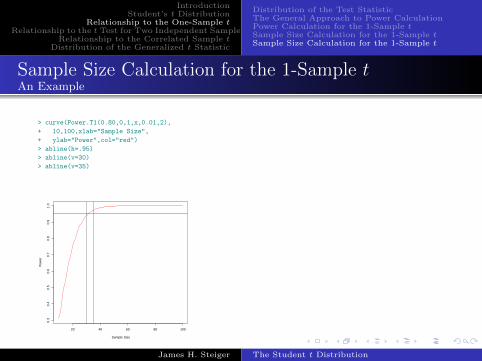
Let’s try calculating the required sample size to achieve apower of 0.95 when Es = 0.80, and the test is two-sidedwith α = 0.01. We’ll use the graphical approach. Here is apreliminary plot. Notice again that Es can be inputdirectly by setting µ0 = 0 and σ = 1 and setting µ = Es.In a couple of seconds, we have the required n narroweddown to between 30 and 35.







> curve(Power.T1(0.80,0,1,x,0.01,2),



> abline(h=.95)

> abline(v=30)

> abline(v=35)

20 40 60 80 100

0.3

0.4

0.5

0.6

0.7

0.8

0.9

1.0

Sample Size

Pow

er








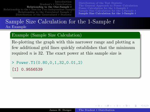
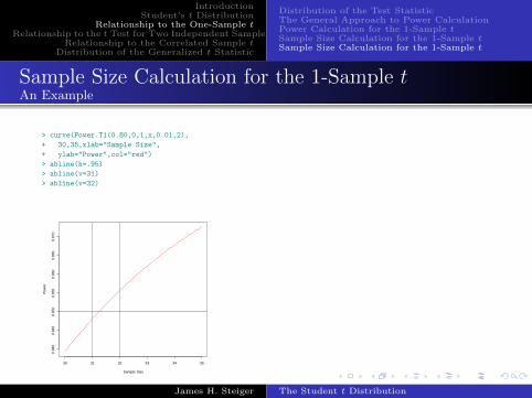
Re-plotting the graph with this narrower range and plotting afew additional grid lines quickly establishes that the minimumrequired n is 32. The exact power at this sample size is

> Power.T1(0.80,0,1,32,0.01,2)

[1] 0.9556539







> curve(Power.T1(0.80,0,1,x,0.01,2),



> abline(h=.95)

> abline(v=31)

> abline(v=32)

30 31 32 33 34 35

0.94

00.

945

0.95

00.

955

0.96

00.

965

0.97

0

Sample Size

Pow

er








GPower automates the process, and yields the identical answer,as shown below.





Distribution of the Test StatisticPower Calculation for the 2-Sample tSample Size Calculation for the 2-Sample t


Earlier, we took the general characterization of the1-sample t and, with a little algebraic manipulation, weshowed that the general distribution of the statistic isnoncentral t with a noncentrality parameter δ that is asimple function of Es and n.The 2-sample t for two independent groups is used tocompare the difference between two population means witha target value that is usually zero. It is calculated as

tn1+n2−2 =Y •1 − Y •2 − κ0√

wσ2(7)

where κ0 is the null-hypothesized value of µ1 − µ2,

w =1

n1+

1

n2=n1 + n2

n1n2(8)

and

σ2 =(n1 − 1)s2

1 + (n2 − 1)s22

n1 + n2 − 2(9)







By a process similar to our derivation in the 1-sample case,we may show that the general distribution of the 2-samplet statistic is noncentral t, with degrees of freedom equal toν = n1 + n2 − 2, and noncentrality parameter given byδ =√w−1Es =

√(n1n2)/(n1 + n2)Es. Es is the

standardized effect size, again, the amount by which thenull hypothesis is wrong, re-expressed in standarddeviation units, i.e.,

Es =µ1 − µ2 − κ0

σ(10)

Notice that, if the sample sizes are equal to a common n,then δ =

√n/2Es.







Power calculation for the 2-Sample t is straightforward.Here is a compact function for the calculations.Note how this function draws on a general purposefunction for computing power with the t distribution thatwe defined earlier.

> Power.T2 <- function(mu1,mu2,sigma,n1,n2,alpha,

+ tails,hypo.diff=0){

+ delta = sqrt((n1*n2)/(n1+n2))*

+ (mu1-mu2-hypo.diff)/sigma

+ return(Power.T(delta,n1+n2-2,alpha,tails))

+ }







Suppose we wish to calculate the power to detectEs = 0.50, when n1 = n2 = 20, α = .05, and the test is2-sided.Again, note how we “trick” the power analysis function byentering µ2 = 0, σ = 1, and replacing µ2 with Es.

> Power.T2(0.50,0,1,20,20,0.05,2)

[1] 0.337939







Clearly, the power with n = 20 per group is not adequate,and we could proceed as before to determine a sample sizeper group that would yield a desired level of power.Sample size planning in the case of two independent groupsis rendered slightly more complicated than in the case of asingle sample, because in some cases it is substantiallyeasier to get participants from one group than from theother.Suppose, for example, you were planning to compare µ1

and µ2 in two independent groups of men and women, butin your participant pool, women outnumber men by a 2 to1 ratio.Moreover, because of time constraints, you cannot afford toinvest the extra time equalizing the sizes of your twosamples.How would you proceed? (Assume desired power is 0.95,α =, 05, 2-sided test.)






Sample Size Calculation for the 2-Sample tUnequal Group Proportions

The simple solution is to “tell the program” you are goingto have unequal sample sizes.GPower offers you the choice of setting an “allocationratio” of n2/n1, and selects sample sizes for both groups onthat basis.Graphically, using R, we could proceed as follows. (Thereare several closely related methods we might try.)







> curve(Power.T2(0.50,0,1,x,2*x,0.05,2),

+ 75,100,col="red",xlab="n1 = n2/2",ylab="Power")

> abline(h=0.95)

75 80 85 90 95 100

0.94

0.95

0.96

0.97

0.98

n1 = n2/2

Pow

er







In a few seconds, we can determine that n1 = 79 andn2 = 158 will produce power slightly exceeding 0.95.In fact, we still would have power slightly exceeding 0.95 ifwe dropped n2 to 157.However, given the guesswork involved and the probabilityof at least minor assumption violations, such hairsplittingseems unnecessary and, indeed, somewhat pedantic.







In the correlated sample t statistic, n observations areobserved for two groups.These observations represent either matched (or correlated)samples, or repeated measures on the same individuals.The correlated sample t statistic is actually a 1-sample tcalculated on the difference scores.The null hypothesis compares the mean of the differencescores with a hypothesized mean difference κ0, whichusually is set equal to zero.Consequently, the distribution of the correlated sample t isnoncentral t, with n− 1 degrees of freedom, and anoncentrality parameter of

δ =√nE∗

s =√nµ1 − µ2 − κ0

σdiff(11)






Distribution of the Correlated Sample t StatisticA Caveat

Clearly, we can process the power and sample sizecalculations for the correlated sample t with essentially thesame mechanics as we used for the 1-sample t. You willnote that the GPower input dialog for the correlatedsample test looks virtually identical to the input dialog forthe 1-sample test.However, it is important to realize that, in a conceptualsense, the “standardized effect size” we input in the2-sample correlated sample test is not the same as in the2-sample independent sample case. This is why I marked itwith an asterisk.







Let’s compare having two independent groups of equal sizen, and taking two repeated measures on one group of sizen. In the former case, the total n is ntotal = 2n, while inthe latter case ntotal = n.In the correlated sample case, if we make a simplifyingassumption of equal variances on each measurementoccasion, we have

σ2diff =

1

n

(σ2 + σ2 − 2ρσ2

)=

1

n2σ2(1− ρ) (12)

So, in terms of the quantities used in the 2-sample test forindependent samples, we see that (assuming equal samplesof size n and a κ0 of zero),

1 Degrees of freedom are n− 1 in the correlated sample case,2(n− 1) in the independent sample case







The noncentrality parameter is

δ =√n/2(µ1 − µ2)/σ =

1

2

√ntotal(µ1 − µ2)/σ

in the independent sample case, and

δ = (1/√

2(1− ρ))√ntotal(µ1 − µ2)/σ

in the dependent sample case.So if we define Es = (µ1 − µ2)/σ, then in the independentcase the actual noncentrality parameter isδ =√ntotal(1/2)Es, while in the dependent case it is

δ =√ntotal(1/

√2(1− ρ))Es. So, for example, if ρ = 0.50,

we have δ = 0.5√ntotalEs in the independent case, and

δ =√ntotalEs in the dependent sample case. For the same

effect size and total sample size, δ will be twice as large inthe dependent sample case.Degrees of freedom in the independent sample test arentotal − 2 and in the dependent sample case degrees offreedom are ntotal − 1.







Notice that, in both cases, the standardized effect we areusually interested in from a substantive standpoint is(µ1 − µ2)/σ, and so the actual power in the correlatedsample test may be higher than in the comparableindependent sample case, provided ρ is positive.The relative power depends on whether the gain in δ offsetsthe halving of the degrees of freedom.In the repeated measures case, the potential gain in poweris often accompanied by a reduction of the number ofparticipants.However, one must be on guard against possible order andhistory effects when planning the administration of therepeated measures.







As an example, suppose that, in the population,(µ1−µ2)/σ = 0.30, α = 0.05, and we desire a power of 0.90.Repeated measurements are expected to correlate 0.70.We first calculate the required sample size under thesupposition that we are taking two independent samples ofsize n. Routine power calculations reveal that, for eachgroup, a sample of n = 235 is required.In the repeated measures case, however, the “effective Es”is 0.30/

√2(1− 0.70) = 0.3872983 in what is essentially a

1-sample t. It turns out that one only needs a sample ofsize n = 72 to be measured on two occasions to attain thepower of 0.90. So the total number of participants isreduced from 470 to 72, and the number of observations isreduced from 470 to 144.GPower draws attention to the fact that one needs tocalculate this somewhat different effect size. One clicks ona Determine key, which opens up a separate dialog.






Distribution of the Correlated Sample t StatisticAssumptions

The assumptions for the correlated sample t test are a bitdifferent from those of the 2-sample independent sampletest.The correlated sample test requires the assumption ofbivariate normality, which is a stronger condition thanhaving data in each condition be normally distributed.The correlated sample test, on the other hand, does notrequire the assumption of equal variances, because the twosets of observations are collapsed into one prior to the finalcalculations.





Distribution of the Generalized t Statistic

Recall that the generalized t statistic for testing the nullhypothesis κ =

∑Jj=1 cjµj = κ0 may be written in the form

tν =K − κ0√Wσ2

(13)

where W =∑

j c2j/nj , and K =

∑j cjX•j .

If we define Es, the standardized effect size as

Es =κ− κ0

σ(14)

then, using the exact same approach we used with the1-sample t, we may show easily that the distribution of thegeneralized t statistic is noncentral t, with degrees offreedom n• − J , and noncentrality parameter

δ = W−1/2Es = W−1/2κ− κ0

σ(15)

It is then a straightforward matter to write a generalroutine to calculate power for the generalized t statistic.





Power Calculation for the Generalized t

Here is simplified code for the power calculation.Note how it draws on the functions we establishedpreviously.

> Power.GT <- function(mus,ns,wts,sigma,alpha,

+ tails,kappa0=0){

+ W = sum(wts^2/ns)

+ kappa = sum(wts*mus)

+ delta = sqrt(1/W) * (kappa-kappa0)/sigma

+ df = sum(ns)-length(ns)

+ return(Power.T(delta,df,alpha,tails))

+ }

To apply the function, we simply input a vector of means,sample sizes, weigthts, and the population standarddeviation. Here is an example in which the average of twoexperimental groups is compared to a control.

> Power.GT(c(75,75,70),c(10,10,10),c(1/2,1/2,-1),10,0.05,2)

[1] 0.2380927

Is there an alternative (better?) way of thinking about thiscalculation in terms of a standardized effect size, ratherthan inputting vectors of means?


the student t distribution - statpower notes/tdistribution.pdf · introduction student’s t...

Documents