introduction to regression and correlation - statpower slides/regressionintro.pdftwo bivariate...
TRANSCRIPT

Regression AnalysisSome Examples
Revisiting Basic Regression ResultsAnscombe’s Quartet
Smoothing the Mean FunctionThe Scatterplot Matrix
Two Bivariate Regression ModelsWhere from Here?
Introduction to Regression and Correlation
James H. Steiger
Department of Psychology and Human DevelopmentVanderbilt University
P312, 2011
James H. Steiger Introduction to Regression and Correlation

Regression AnalysisSome Examples
Revisiting Basic Regression ResultsAnscombe’s Quartet
Smoothing the Mean FunctionThe Scatterplot Matrix
Two Bivariate Regression ModelsWhere from Here?
Introduction to Regression and Correlation1 Regression Analysis
Introduction
2 Some Examples
Inheritance of Height
Temperature, Pressure, and the Boiling Point of Water
3 Revisiting Basic Regression Results
Introduction
Covariance, Variance, and Correlation
The OLS Best-Fitting Straight Line
Conditional Distributions in the Bivariate NormalDistribution
Mean Functions
Variance Functions
4 Anscombe’s Quartet
5 Smoothing the Mean Function
6 The Scatterplot Matrix
7 Two Bivariate Regression Models
8 Where from Here?
James H. Steiger Introduction to Regression and Correlation

Regression AnalysisSome Examples
Revisiting Basic Regression ResultsAnscombe’s Quartet
Smoothing the Mean FunctionThe Scatterplot Matrix
Two Bivariate Regression ModelsWhere from Here?
Introduction
Introduction to Regression Analysis
Regression is the study of dependence. It is used to answer suchquestions as:
1 Do changes in diet result in changes in cholesterol level?2 Does an increase in the size of classes result in a reduction
in learning?3 Can a runner’s marathon time be predicted from her 5km
time?4 What factors in an insurance company’s database can be
used to successfully predict whether a claim is fradulent?
James H. Steiger Introduction to Regression and Correlation

Regression AnalysisSome Examples
Revisiting Basic Regression ResultsAnscombe’s Quartet
Smoothing the Mean FunctionThe Scatterplot Matrix
Two Bivariate Regression ModelsWhere from Here?
Introduction
Goals of Regression Analysis
1 The goal of regression is to summarize observed data in asimple, elegant, and useful way.
2 Our simplest examples will involve two variables, one ofwhich is predicted from the other.
3 We’ll now look at a few examples, using a tool that itabsolutely essential for the analysis of regression data – thescatterplot.
James H. Steiger Introduction to Regression and Correlation

Regression AnalysisSome Examples
Revisiting Basic Regression ResultsAnscombe’s Quartet
Smoothing the Mean FunctionThe Scatterplot Matrix
Two Bivariate Regression ModelsWhere from Here?
Inheritance of HeightTemperature, Pressure, and the Boiling Point of Water
Inheritance of Height
One of the first uses of regression was to study inheritanceof traits from generation to generation.During the period 1893–1898, E. S. Pearson organized thecollection of n = 1375 heights of mothers in the UnitedKingdom under the age of 65 and one of their adultdaughters over the age of 18.Pearson and Lee (1903) published the data, which are inthe data file heights.txt.
James H. Steiger Introduction to Regression and Correlation

Regression AnalysisSome Examples
Revisiting Basic Regression ResultsAnscombe’s Quartet
Smoothing the Mean FunctionThe Scatterplot Matrix
Two Bivariate Regression ModelsWhere from Here?
Inheritance of HeightTemperature, Pressure, and the Boiling Point of Water
Inheritance of Height
The alr3 library must be loaded before we begin. We start byloading the data and attaching it.
> data(heights)> attach(heights)
James H. Steiger Introduction to Regression and Correlation

Regression AnalysisSome Examples
Revisiting Basic Regression ResultsAnscombe’s Quartet
Smoothing the Mean FunctionThe Scatterplot Matrix
Two Bivariate Regression ModelsWhere from Here?
Inheritance of HeightTemperature, Pressure, and the Boiling Point of Water
Producing the Scatterplot
Next, we produce a scatterplot showing the height of thedaughter (Dheight) and the height of the mother (Mheight).
> plot(Mheight,Dheight,xlim=c(55,75),ylim=c(55,75),pch=20,cex=.3)
●
●
●
●
●
●
●
●
●
●
●
●
●
●
●
● ●
●
●
●
●
●
●
●
●●
●
●
●
●
●
●
●
●
●
●
●●
●●
● ●
●
●
●
●
●
●
●
●
●
●
●
●
●
●
● ●
●
●
●
● ●
●
●
●
●
●
●
●
●
●●
●
●
●
●
●
●
●
●
●
●
●
● ●
●
●
●●
●
●
●
●
●
●
●
●
●
●
●
●
●
●
●
●
●
●
●
●
●●
●
●
●
●
●
●
●
●
●● ●
●
●
●●
●
●
●
●
●
●
●
●
●
●
●
●
●
●
●
●
●●
●
●
●
●
●●
●
●
●
●
●
●
●
●
●
●
● ●●
●
●
●
● ●
●
●
●
●
●
●
●
●
●
●
●
●
●
●
●
●
●
●
●
●
●
●
●
●
●
●
●
●
●
●
●
●
●
●
●
●
●
●
●
●
●
●
●
●
●
●
●
●
●
●
●●
●
●
●
●
●
●
●
●
●
●
●
●
●●
●
●
●
●
●
●
●
●
●
●
●
●
●
●
●
●
●
●
●
●
●
●
●
●
●
●
●
●
●
●
●
●
●
●
●
●
●
● ●
●
●
●
●
●
●
●
●
●
●
●
●
●
●
●
●
●
●
●
●
●
●
●
●
●
●
●
●
●
●
●
●
●
●
●
●
●
●
●
●
●
●
●
●
●●
●
●
●
●● ●
●
●
●
●
●
●
●
●
●
●
●
●
●
●
●
●
● ●
●
●
●
●
●
●
●
●
●
●
●
●
●
●
●
●●
●
●
●
●
●
●
●
●
●
● ● ● ●
●
●
●
●● ●
●
●
●
●
●
● ●
●
●
●
●
●
●
●
●
●
●
●●
●
●
●
●
●
● ●
●
●
●●
●
●
●
●
●
●
●
●
●
● ●
●
●
●
●
●
●
●●
●
●
●
●
●
●
●
●●
●
●
●
●
●
●
●
●
●
●
●
●
●
●
●
●
●
●
●
●
●
●
●
●
●
●
●
●
●●
●
●
●
●
●
●
●
● ●
●
●
●
●
●
●
●
● ●
●
●
● ●
● ●
●
●
●
●● ●
●●
●
●
●
●
●
●
●
●
●
●
●
●
●
●
●
●
●●
●
●
●
● ●
●
●
●
●
●
● ●
●
●
●
●
●
●
●
●
●
●
●
●
●
●
●
●
●
●
●
●
●
●
●
●
●
●
●
●
●
●
●
●
●
●
●
●
●
● ●
●
●
●
●
●
●
●
●
●
●
●
●
●
●
●●
●
●
●
●
●
● ●
●
●
●
●
●
●
●
●
●
●
●
● ●
●
●
●
●
●
●
●
●
●
●
●
●
●
●
●
●
●
●
●
●
●
●
●
●
●
●
●
●
●
●●
●
●
●
●
●
●
●
●
●
●
●●
●
●
● ●
●
●
●
●
● ●
●
●
●
●
●
●
●
●
●
●
●
●
●
●
● ●
●
● ● ●
●
●
●
●
●
●
●
●
●
●
●
●
●
●
●
● ●
●
●
●
●
●
●
●
●
●
●
●
●
●
●
●
●
●
●
●
●
●
●
●
●
●
●
●
●
●
●
●
●
●
●
●●
●
●
●
●
●
●
●
●
●
●
●
●
●
●
●
●
●
●
●
●
●
●●
●
●
●
●
●
●
●
●
●
●
●
●
●
●
●
●
●
●
●
●
● ●
●
●
●
●
●
●
●
●
●
●●
●
●
●
●
● ●
●
●
●
●
●
●
●
●
●●
●
●
●
●
●
●
●
●
●
●
●
●
●●
●
●
●
●●
●
●
●
●
●
●
●●
●
●
●
●
●
●
●
●
●●
●
●
●
●
●
●
●
●●
●●
●
●
●
●
●
●
●
●
●
●
●
●
●
●
●
●
●
●
●
●
● ●
●
●
● ●
●●
●
● ●
●
●
●●
●
●
●
●
●
●
●
●
●
●
●
●
●
●
●
●
●
●
●
●
●
●
●●
●
●
●
●
●
●
●
●
●
●
●
●
●
● ●
●
●
●
●
●
●
●
● ●
●
●
●
●
●
●
●
●
●
●
●
●
●
●●
●●
●
●
●
●
●
●
●
●
●●
●
●
●
●
●
●
●
●
●
● ●
●
●
●
●
●
●
●
●
●
●
●
●
●
●
●
●
●
●
●
●
●
●
●
●
●
●
●
●
●
●
●
●
●
●
●
●
● ●
● ●
●
●
● ●
●
●●
●
●
●
●
●
●
●
●
●
●
●
●
●
●●
●
●
●
●
● ●
●
●
●
●
●
●
●
●
●
●
●
● ●
●
●
●
●
●
●
●
●
●
●
●
●●
●
●
●
●
●
●
●
●
●
●
●
●
●
●
●
●
●
●
●
●
●●
●
●
●
●
●
●
●
●
●
●
●
●
●
●
●
●
●
●
●
●
●
●
●
●
●
●
● ●
●
●
●
●
●
●
●
●
●
●
●
●
●
●●
●
●
●
●
●
●
●●
●
●
● ●
●
●
●
●
●
●
●
●
● ●
●
●
●●
●
●
●
●
●
●
●
●
●
●
●
●
●
●
●
●
●●
●
●
●
●
●
●
●
●
●
●
●
●
●
●
●
●
●
●
●
●
●
●
●
●
●
●
●
●
●
●
●
●
●
●
●
●●●
●
●
●
●
●
●●
●
●
●
●
●
●
●
●
● ●
●
●
●
●
●
●
●
●
●
●
●
●
●
●
●
●
●
● ●
●
●
●
●
●
●
●
●
●
●
●
●
●
●
●
●
●
●
●
●
●
●
●
●
● ●
●
●
●
●
●
●
●●
●
●
● ●
●
●
●
●
●●
●
● ●
●
●
●
● ●
●
●
● ●
●
●
●
●
●
●
●
●
●
●●
●●
●
●
●
●
●
●
●
● ●
● ●
●
●
●
●
●
●
●
●
●
●
●
●
●
●
●
●
●
●
●
●
●
●
●
●
●
●
●
●
●
● ●
●
●
●
●
●
●
●
●
●
●
●
●
●
●
●
55 60 65 70 75
5560
6570
75
Mheight
Dhe
ight
James H. Steiger Introduction to Regression and Correlation

Regression AnalysisSome Examples
Revisiting Basic Regression ResultsAnscombe’s Quartet
Smoothing the Mean FunctionThe Scatterplot Matrix
Two Bivariate Regression ModelsWhere from Here?
Inheritance of HeightTemperature, Pressure, and the Boiling Point of Water
Producing the Scatterplot
Some comments are in order.
The range of heights appears to be about the same formothers and for daughters.Because of this, we draw the plot so that the lengths of thehorizontal and vertical axes are the same, and the scalesare the same. We forced this by use of the xlim and ylimoptions.Some computer programs automate the sizing of the X andY axes, but others may require you to do this for yourself.Fortunately, in R it is very easy to experiment.
James H. Steiger Introduction to Regression and Correlation

Regression AnalysisSome Examples
Revisiting Basic Regression ResultsAnscombe’s Quartet
Smoothing the Mean FunctionThe Scatterplot Matrix
Two Bivariate Regression ModelsWhere from Here?
Inheritance of HeightTemperature, Pressure, and the Boiling Point of Water
Jittering the Scatterplot
Weisberg tells us in the text that the original data aspublished were rounded to the nearest inch.In order to avoid an unfortunate problem with suchrounded data, Weisberg displaced the data randomly in theX and Y directions by using a uniform random numbergenerator on the range from −0.5 to +0.5, then roundingto a single decimal place.This type of operation is called jittering the scatterplot.What problem was he fixing?
James H. Steiger Introduction to Regression and Correlation

Regression AnalysisSome Examples
Revisiting Basic Regression ResultsAnscombe’s Quartet
Smoothing the Mean FunctionThe Scatterplot Matrix
Two Bivariate Regression ModelsWhere from Here?
Inheritance of HeightTemperature, Pressure, and the Boiling Point of Water
Jittering and Un-jittering
We can round the data back to the nearest inch by usingthe round function in R. This will give us an idea of whatwe would see if we did not jitter the plot.Let’s do that, then plot the rounded variables, and seewhat the new scatterplot looks like. Code is shown below.
James H. Steiger Introduction to Regression and Correlation

Regression AnalysisSome Examples
Revisiting Basic Regression ResultsAnscombe’s Quartet
Smoothing the Mean FunctionThe Scatterplot Matrix
Two Bivariate Regression ModelsWhere from Here?
Inheritance of HeightTemperature, Pressure, and the Boiling Point of Water
Jittering and Un-jittering
> X<-round(Mheight)> Y<-round(Dheight)> plot(X,Y,xlim=c(55,75),ylim=c(55,75),pch=20,cex=.3)
●
● ●
●
●
●
●
●
●●
●
●
● ●
●
● ●●
●
●●
●
●
●
●●
●●●
●
●●
●
●
●
●
●●
●●● ●●
● ●●
●
●
●
●●
●
●
●
●
●● ●
●●
● ●●●● ●● ●
●
●
●
●●
●
●●
● ●●
●
●
●
●●
● ●
●
●●●
●
●
●
●
● ●
●
●
●
● ●
●
●●
●
●
●●
●●
●●
● ●●
●
●●
●
●
●● ●
●
●
●● ●●●● ●●
●
●● ●
●
●●●
●
● ●●
●●
● ●●●●
●
●
●●
●
●
● ●●
●●●
●●●
● ●
●
●
●●●
●
●●●
●● ●
●
●●
●
●
●
●
●● ●●●
●●
●
●
●●
●
●
●●
●
●
●
●
●●
● ●
●
●
●●●
●
●●
●●●
●
●
● ●●
●● ●● ●
● ●●
●
●
●
●
● ●●
●●●●
●
●
●●●
●●●● ●
●
●
●●
●●●●● ●
●
●
●● ●
●
●●
● ●
●
●
●
●●● ●●
●
●
●●●
●●●
● ●
●●
●
●●
● ●
●
● ●
●●
●
●
●
●●
●● ●●
●●
●
●●●
●
●
●●●
●
●●
●
● ●
● ●
●
●● ●
●
●●
●
● ●● ●
●
● ●
●
● ●
●
●●
●
●●
●
●●●●● ●●●
●
●
● ●●● ●
●●
●
●● ●●
●
●●
●
●●
● ●
●
●
●
●
●●
●●●●
●●●
●●
●●●
●
●● ●
● ●
●●
●
●●●● ●● ●●
●
●●●●● ●
●
●
●
●● ●●
●
●
●
●●●
●
●
●
●
●
●
●●
●●
●●
●
●
●
● ●
●● ●
●●
●●●
●
●
●●●
●
●●●
● ●●
●
●●●●●●
●●
● ●●●●●● ● ●●●
● ●
● ●●
●
●●● ●
●
●
●
●●
●●●
●● ●●
●
●
●
●
●
●●
●
●
●
●
●●
●
●
●
● ●
●●
●●
● ●
●●
●
●
●● ●●
●●
●●●
●●
●●
●●
●
● ●●
●●
●
●
●
●
●
●
●
●● ●
● ●●●
●●
●●●●
● ●
● ●
●
●●
●●●●●●
●
● ●
●
●
●
●●
●
● ●●
●●● ●
●●●●
●
●
●
●
●
●
●
●
●
●●●● ●
●
●
●
●
●●●●● ●●
● ●
●● ●
●
●●
●●
●●
●● ●●
●
●
●
●
●
●
● ●
●●● ●
●●
● ●●
●● ●
● ●●●
●
●
●
● ●
●● ●
●
● ●
●
●●
●
●●
●
●●●
●
●
●● ●
● ●●●●
●
● ●●● ●
●●
●●
● ● ●●
●
●●
●
●●
●●
●
●●
●●
●
●●●●●
●●●
●
●
●
●
●
●●
●●● ●
●
●●
●●
●● ●
●
●
●
●
●●
●
●
●
●● ●
●●
●●●● ●
●
●●
●●●
●●
●●
●
● ●●●● ●
●
●● ●● ●
●
●●●
●
●●●● ●
●●
●●●
●
●
●
●
●
●●
●
●● ●
●
●
●
●●
●● ●●
●● ●
●●
●
●
●●
●
●●
●
●
●
●
●
●●●
●
●●●
●●
●
●●
●
●
●●● ●
●
●●●●●●
●●
● ●●●●●●● ●
●
●●●● ●
●
●●●
●●
●
●
●●
●● ●
● ●● ●●
●
●●● ●
●
● ●●
●
●
●●
●
● ●
●
●●
●●●●
●●● ●●●●●●●
●●
● ●
●●
● ● ●●● ●●●
●●●● ●
●●
●
●
●
●
●●●
●
●● ●
●●
●
●
●
●
●●
●
●
●
●
●
● ●
● ●
●
●● ●
●
●●
● ●
●●
●
● ●
●
●
●
●● ●●● ●
●●
●
● ●●●●
●●
●
●
●●●●
●●
● ●
●
● ●●● ●●●
●
●●
●●● ●● ●
●●● ●
●
●
●●●●● ●
●
●
●●
●
●
●
●
●
● ●● ●●
●
●
●●●
●
●●
●
● ●● ●
●
●●●●
●
●
●●
●
●
●●
●●●●
● ●●
●●
● ●●
●
●●●● ●● ●
●
●
●
● ●
●
●●●●●●●
●●
●● ●
●
●●
●●
● ●
● ●
●
●
●●
●
●
●●
●●
● ●
●
●●
●●
●
●
●
● ●● ●●
●
● ●
●
●●
●●
●
●
●●
●
● ●●●●
●
●●●
●●
●
●
● ●●
●
●
● ● ●
●
●●
●●
● ●
●
●
●
●●●
●
●
●
●● ●●●●
●
●
● ●●
●
●
● ●●
●
●
●
●●
●
●● ● ●
● ●●● ●●
●
●
● ●● ● ●
●●●
●●●
●●
●
● ●
●
●
●
● ●●●
●●●
●● ●
●●●
● ●●● ●●
●
●
●●
●●
●
●●
●●●●
●●
● ●● ●
●
● ●
● ●●
● ●
●
●●
●
●
● ●
●
● ●●
●●● ●
●
●
●
●
●
●
●
●
●
●●
●
● ●
●
55 60 65 70 75
5560
6570
75
X
Y
James H. Steiger Introduction to Regression and Correlation

Regression AnalysisSome Examples
Revisiting Basic Regression ResultsAnscombe’s Quartet
Smoothing the Mean FunctionThe Scatterplot Matrix
Two Bivariate Regression ModelsWhere from Here?
Inheritance of HeightTemperature, Pressure, and the Boiling Point of Water
Jittering and Un-jittering
R has a built-in jitter functionLet’s try it with our rounded data.
James H. Steiger Introduction to Regression and Correlation

Regression AnalysisSome Examples
Revisiting Basic Regression ResultsAnscombe’s Quartet
Smoothing the Mean FunctionThe Scatterplot Matrix
Two Bivariate Regression ModelsWhere from Here?
Inheritance of HeightTemperature, Pressure, and the Boiling Point of Water
Jittering and Un-jittering
> X.jittered <- jitter(X,amount=.5)> Y.jittered <- jitter(Y,amount=.5)> plot(X.jittered,Y.jittered,xlim=c(55,75),ylim=c(55,75),pch=20,cex=.3)
●
●
●
●
●
●
●
●
●
●
●
●
●
●
●
●
●
●
●
●
●
●
●
●
●
●
●
●
●
●
●
●
●
●
●
●
●●
●
●
●
● ●
●
●
●
●
●
●
●
●
●
●
●
●
● ●
●
●
●
●
●
●
●
●
●
●
●
●
●
●
●
●
●
● ●
●
●
●
●
●
●
●
●
●
●
●
●
●
●
●
●
●
●
●
●
●
●
●
●
●
●
●●
●
●
●●
●
●
●
●
●
●
●
●
●
●
●
●
●●
●
●
●
●
●
●●●
●
●
●
●
●
●
●●
●
●
●
●
●●
●
●
●
●
●
●
●
●
●
●
●
●
●
●
●
●
●
●
●
●
●●
●
●
●
●
●
● ●
●
●
●
●●
●
●
●
●
●
●
●
●
●
●
●
●
●
●
●
●
●
●
●
●
●
●
●
●
●
●
●
●
●
●
●
●
●
●
●
●●
●
●
●
●
●
●
●
●
●
●
●
●
●
●
●
●
●
●
●
●
●
●
●
●
●
●
●
● ●
●
●
●
●
●
●
●
●
●
●●
●
●
●
●
●
●●
●●
●
●
●
●
●
●
●
●
●
●
●
●
●
●
●
●
●
●
●
●
●
●
●●●
●
●
●
● ●
●
●
●
●
●
●●
●
●
●
●
●
●
●
●
●
●
●
●
●
●
●
●
●
●
●
●
●
●
●
●
●
●
●
●
●
●
●
●●
●
●
●
●
●
●
●
●
●
●
●
●
●
●
●
●
●
●
●
●
●
●
●
●
●
●
●
●
●●
●
●
●
●
●
●
●
●●
●
●●
●
●
●
●
●
●
●●
●
●
●
●●
●
●
●
●
●
●
●
●
●●
●
●
●
●
●
●
●
●
●
●
●
●
●
●
●●
●
●●
●
●●
●
●
●
●
●
●
●
●
●
●
●
●
●
●
● ●
● ●
●
●
●
●
●
●
●
●
●
●
●
●
●
●
●
●
●
●
●
●
●
●
●
●
●
●
●
●
●
●
●
●
●
●●
●
●
●●
●
●
●
●
●
●●
●
●
●
●●
●
●
●
●
●
●●
●
●
●●
●
●
●
●
●
●
●●
●
●
●
●
●
●
●
●
●●
●
●
●●
●
●
●
●
●
●●
●
●
●
●
●
●
●
●
●
●
●
●
●
●
●
●
●
●
●
●
●
●
●
●
●
● ●
●
●
●
●
●
●
●
●
●
●
●
●●
●
●
●
●
●
●
●
●
●
●●
●
●
●
●
●
●
●
●
●●
●
●
●
●
●
●
●
●
●
●
●
● ●
●
●
● ●
●
●
●
●
●
●
●
●
●
●
●
●
●
●
●
●
●
●
●
●
●
●
●
●
●
●
●
●
●
●
●
●
●
●
●
●
●
●
●
●
●
●
●
●
●
●
●
●
●
●
●
●
●
●
●
●
●●
●
●
●
●
●
●
●
●
●
●●
●
●
●
●
●
●
●●
●
●
●
●
●
●
●
●
●
●
●
●
●
●
●
●
●
●
●
●
●
●
●
●
●
●
●
●
●
●
●
●
●
●
●
●
●
● ●
●
●
●
●
●
●
●
●
●
●
●
●
●
●
●
●
●
●
●
●
●
●
●
●
●
●
●●
●
●
●
●
●
●
●
●
●
●
●
●
●
●
●
●
●
●
●
●
●
●
●●
●
●
●
●
●
●
●
●
●
●● ●
●
●
●
●
●
●
●
●
●
●
●
●
●
●
●
●
●
●
●
●●
●
●●
●
●
●
●
●
●
●
●
●
●
●
●
●
●
●
●
●
●
●
●
●
●
●
●
●
●
●
●
●
●
●●
●
●
●
●●
●
●
●
●
●●
●
●
●
●
●
●
●
●
●
●
●
●
●
●
●
●
●
●
●
●
●
●
●
●
●
●
●
●
●
●
●●
●
●
●
●
●●
●
●
●
●
●
●
●
●●
●●
●
●
●
●
●●
●
●
●
●
●●
●
●
●
●
●●
●●
●
●
●●
●
●
●
●
●
●
●
●
●
●
●
●
●
●
●
●
●
●
●
●
●
●●
●
●
●●
●
●
●
●●
●
●●
●
●
●
●
●
●
●
●
●●
●
●
●
●
●
●
●●
●
●
●
●
●
●
●
●
●
●
●
●
●
●
●
●
●
●
●
●
●
●
●
●
●
●
●
●
●
●●
●
●
●
●
●
●
●
●
●
●
●
●
●
●
●
●
●
●
●
●
●
●
●
●
●
●
●
●●
●
●
●
●
●
●
●●
●
●
●
●
●●
●
●
●
●
●
●
●
●
●
●
●
●
●
●
●●
●
●
●
●
●
●
●
●● ●
●
●
●
●
●
●
●
●
●
●
●
●
●
●
●
●
●
●
●
●
●
●
●
●
●
●
●
●
●
●
●
●
●
●
●
●
●
●
●
●
●
●
●
●
●
●
●
●
●
●
●
●
●
●
●
●
●●
●
●
●
●
●
●
●
●
●
●
●
●
●
●
●
●
●
●
●●
●
●
●
●
●
●
●
●
●
●
●
●
●
●
●
●
●
●
●●
●
●
●
●
●
●
●
●
●
●
●
●
●
●
●
●
●
●
●
●
●
●
●
●
●
●
●
●
●
●
●
●
●
●
●
●
● ●
●
●
●
●
●
●
●
●
●
●
●
●
●
●
●
●
●
●
●
●
●
●
●
●
●
●
●
●
●
●
●
●●
●
●
●
●
●
●●
●
●
● ●
●
●
●
●
●●
●
●
● ●
●
●
●
●
● ●
●
●
●
●
●●●
●
●
●
●
●
●
●
●
●
●
●
●
●
●
●
●
●
●
●
●
●
●
●
●
●
●
●
●
●
●
●
●
●
●
●
●
●
●
●
●
●
●
●
●
●
●
●
●●
●
●
●●
●
●
●
●
●
●
●
●
●
●●
●
●
●
●
●
●
●
●
●
●
●
●
●
●
●
●
●
●
●
●
●
●
●
●
●
●
●
55 60 65 70 75
5560
6570
75
X.jittered
Y.jit
tere
d
James H. Steiger Introduction to Regression and Correlation

Regression AnalysisSome Examples
Revisiting Basic Regression ResultsAnscombe’s Quartet
Smoothing the Mean FunctionThe Scatterplot Matrix
Two Bivariate Regression ModelsWhere from Here?
Inheritance of HeightTemperature, Pressure, and the Boiling Point of Water
Examining the Scatterplot
We examine the scatterplot to see if there is an identifiabledependency.If X and Y were independent, then the conditionaldistribution of Y for a given value of X would not change.This is clearly not the case here since as we move acrossthe scatterplot from left to right, the scatter of points isdifferent for each value of the predictor.
James H. Steiger Introduction to Regression and Correlation

Regression AnalysisSome Examples
Revisiting Basic Regression ResultsAnscombe’s Quartet
Smoothing the Mean FunctionThe Scatterplot Matrix
Two Bivariate Regression ModelsWhere from Here?
Inheritance of HeightTemperature, Pressure, and the Boiling Point of Water
Examining the Scatterplot
●
●
●
●
●
●
●
●
●
●
●
●
●
●
●
● ●
●
●
●
●
●
●
●
●●
●
●
●
●
●
●
●
●
●
●
●●
●●
● ●
●
●
●
●
●
●
●
●
●
●
●
●
●
●
● ●
●
●
●
● ●
●
●
●
●
●
●
●
●
●●
●
●
●
●
●
●
●
●
●
●
●
● ●
●
●
●●
●
●
●
●
●
●
●
●
●
●
●
●
●
●
●
●
●
●
●
●
●●
●
●
●
●
●
●
●
●
●● ●
●
●
●●
●
●
●
●
●
●
●
●
●
●
●
●
●
●
●
●
●●
●
●
●
●
●●
●
●
●
●
●
●
●
●
●
●
● ●●
●
●
●
● ●
●
●
●
●
●
●
●
●
●
●
●
●
●
●
●
●
●
●
●
●
●
●
●
●
●
●
●
●
●
●
●
●
●
●
●
●
●
●
●
●
●
●
●
●
●
●
●
●
●
●
●●
●
●
●
●
●
●
●
●
●
●
●
●
●●
●
●
●
●
●
●
●
●
●
●
●
●
●
●
●
●
●
●
●
●
●
●
●
●
●
●
●
●
●
●
●
●
●
●
●
●
●
● ●
●
●
●
●
●
●
●
●
●
●
●
●
●
●
●
●
●
●
●
●
●
●
●
●
●
●
●
●
●
●
●
●
●
●
●
●
●
●
●
●
●
●
●
●
●●
●
●
●
●● ●
●
●
●
●
●
●
●
●
●
●
●
●
●
●
●
●
● ●
●
●
●
●
●
●
●
●
●
●
●
●
●
●
●
●●
●
●
●
●
●
●
●
●
●
● ● ● ●
●
●
●
●● ●
●
●
●
●
●
● ●
●
●
●
●
●
●
●
●
●
●
●●
●
●
●
●
●
● ●
●
●
●●
●
●
●
●
●
●
●
●
●
● ●
●
●
●
●
●
●
●●
●
●
●
●
●
●
●
●●
●
●
●
●
●
●
●
●
●
●
●
●
●
●
●
●
●
●
●
●
●
●
●
●
●
●
●
●
●●
●
●
●
●
●
●
●
● ●
●
●
●
●
●
●
●
● ●
●
●
● ●
● ●
●
●
●
●● ●
●●
●
●
●
●
●
●
●
●
●
●
●
●
●
●
●
●
●●
●
●
●
● ●
●
●
●
●
●
● ●
●
●
●
●
●
●
●
●
●
●
●
●
●
●
●
●
●
●
●
●
●
●
●
●
●
●
●
●
●
●
●
●
●
●
●
●
●
● ●
●
●
●
●
●
●
●
●
●
●
●
●
●
●
●●
●
●
●
●
●
● ●
●
●
●
●
●
●
●
●
●
●
●
● ●
●
●
●
●
●
●
●
●
●
●
●
●
●
●
●
●
●
●
●
●
●
●
●
●
●
●
●
●
●
●●
●
●
●
●
●
●
●
●
●
●
●●
●
●
● ●
●
●
●
●
● ●
●
●
●
●
●
●
●
●
●
●
●
●
●
●
● ●
●
● ● ●
●
●
●
●
●
●
●
●
●
●
●
●
●
●
●
● ●
●
●
●
●
●
●
●
●
●
●
●
●
●
●
●
●
●
●
●
●
●
●
●
●
●
●
●
●
●
●
●
●
●
●
●●
●
●
●
●
●
●
●
●
●
●
●
●
●
●
●
●
●
●
●
●
●
●●
●
●
●
●
●
●
●
●
●
●
●
●
●
●
●
●
●
●
●
●
● ●
●
●
●
●
●
●
●
●
●
●●
●
●
●
●
● ●
●
●
●
●
●
●
●
●
●●
●
●
●
●
●
●
●
●
●
●
●
●
●●
●
●
●
●●
●
●
●
●
●
●
●●
●
●
●
●
●
●
●
●
●●
●
●
●
●
●
●
●
●●
●●
●
●
●
●
●
●
●
●
●
●
●
●
●
●
●
●
●
●
●
●
● ●
●
●
● ●
●●
●
● ●
●
●
●●
●
●
●
●
●
●
●
●
●
●
●
●
●
●
●
●
●
●
●
●
●
●
●●
●
●
●
●
●
●
●
●
●
●
●
●
●
● ●
●
●
●
●
●
●
●
● ●
●
●
●
●
●
●
●
●
●
●
●
●
●
●●
●●
●
●
●
●
●
●
●
●
●●
●
●
●
●
●
●
●
●
●
● ●
●
●
●
●
●
●
●
●
●
●
●
●
●
●
●
●
●
●
●
●
●
●
●
●
●
●
●
●
●
●
●
●
●
●
●
●
● ●
● ●
●
●
● ●
●
●●
●
●
●
●
●
●
●
●
●
●
●
●
●
●●
●
●
●
●
● ●
●
●
●
●
●
●
●
●
●
●
●
● ●
●
●
●
●
●
●
●
●
●
●
●
●●
●
●
●
●
●
●
●
●
●
●
●
●
●
●
●
●
●
●
●
●
●●
●
●
●
●
●
●
●
●
●
●
●
●
●
●
●
●
●
●
●
●
●
●
●
●
●
●
● ●
●
●
●
●
●
●
●
●
●
●
●
●
●
●●
●
●
●
●
●
●
●●
●
●
● ●
●
●
●
●
●
●
●
●
● ●
●
●
●●
●
●
●
●
●
●
●
●
●
●
●
●
●
●
●
●
●●
●
●
●
●
●
●
●
●
●
●
●
●
●
●
●
●
●
●
●
●
●
●
●
●
●
●
●
●
●
●
●
●
●
●
●
●●●
●
●
●
●
●
●●
●
●
●
●
●
●
●
●
● ●
●
●
●
●
●
●
●
●
●
●
●
●
●
●
●
●
●
● ●
●
●
●
●
●
●
●
●
●
●
●
●
●
●
●
●
●
●
●
●
●
●
●
●
● ●
●
●
●
●
●
●
●●
●
●
● ●
●
●
●
●
●●
●
● ●
●
●
●
● ●
●
●
● ●
●
●
●
●
●
●
●
●
●
●●
●●
●
●
●
●
●
●
●
● ●
● ●
●
●
●
●
●
●
●
●
●
●
●
●
●
●
●
●
●
●
●
●
●
●
●
●
●
●
●
●
●
● ●
●
●
●
●
●
●
●
●
●
●
●
●
●
●
●
55 60 65 70 75
5560
6570
75
Mheight
Dhe
ight
James H. Steiger Introduction to Regression and Correlation

Regression AnalysisSome Examples
Revisiting Basic Regression ResultsAnscombe’s Quartet
Smoothing the Mean FunctionThe Scatterplot Matrix
Two Bivariate Regression ModelsWhere from Here?
Inheritance of HeightTemperature, Pressure, and the Boiling Point of Water
Examining the Scatterplot
We can see this even more clearly in Weisberg’s figure 1.2, inwhich we show only points corresponding to mother-daughterpairs with Mheight rounding to either 58,64, or 68 inches.
We establish a selection condition with the code below.
> sel <- (57.5 < Mheight) & (Mheight <= 58.5) |+ (62.5 < Mheight) & (Mheight <= 63.5) |+ (67.5 < Mheight) & (Mheight <= 68.5)
James H. Steiger Introduction to Regression and Correlation

Regression AnalysisSome Examples
Revisiting Basic Regression ResultsAnscombe’s Quartet
Smoothing the Mean FunctionThe Scatterplot Matrix
Two Bivariate Regression ModelsWhere from Here?
Inheritance of HeightTemperature, Pressure, and the Boiling Point of Water
Examining the Scatterplot
Then we plot the figure.
> plot(Mheight[sel],Dheight[sel],xlim=c(55,75),ylim=c(55,75),pch=20,cex=.3,+ xlab="Mheight",ylab="Dheight")
●
●
●
● ●
●
●
●
●
●
●
●
●
●
●
● ●
●
●
●
●
●
●
● ●
●
●
●
●
●
●
●
●
●
●
●
●
●
●
●
●
●
●
●
●
●
●
●
●
●
●
●
●
●
●
●
●
●
●
●
● ●
● ●
●
●
●
●
●
●
●
●
●
●
●
●
●
●
●
●
● ●
●
●
●
●
●
●
●● ●
●
●
●
●
●
●
●
●
●
● ●
●
●
●
●
●
●
●
●
●
●
●
●
●
●
●
● ●
● ●
●
●
●
●
● ●
●
●
●
●
●
●
●
●
●
●
●
●
●
●
●
●
●
●
●
●
●
●
●
●●
●
●
●
●
●
●
●
●
●●
●
●
●
●
●
●
●
●
●
●
● ●
●
●
●
●
●
●
●
●
●
●
●
●
●
●
●
●
●
●
●
●
●
●●
●
●
●
●●
●
●
●
● ●
●
●
●●● ●
●
●
●
● ●
●
●●
●
● ●
●
●●
●
●
●
●●
●
●
●
●
●
●
●
●
●
●
●
●
●
●
●●
●
●
●
●
●
●
●
●
●
●
●
●
●
●
●
●
●
●
●
●
●
●
●
●
55 60 65 70 75
5560
6570
75
Mheight
Dhe
ight
James H. Steiger Introduction to Regression and Correlation

Regression AnalysisSome Examples
Revisiting Basic Regression ResultsAnscombe’s Quartet
Smoothing the Mean FunctionThe Scatterplot Matrix
Two Bivariate Regression ModelsWhere from Here?
Inheritance of HeightTemperature, Pressure, and the Boiling Point of Water
Examining the Scatterplot
We see that within each of these three strips or slices
The mean of Dheight is increasing from left to right, andThe vertical variability in Dheight seems to be more or lessthe same for each of the fixed values of Mheight in the strip.
James H. Steiger Introduction to Regression and Correlation

Regression AnalysisSome Examples
Revisiting Basic Regression ResultsAnscombe’s Quartet
Smoothing the Mean FunctionThe Scatterplot Matrix
Two Bivariate Regression ModelsWhere from Here?
Inheritance of HeightTemperature, Pressure, and the Boiling Point of Water
Examining the Scatterplot
The scatter of points in the graph appears to be more or lesselliptically shaped, with the axis of the ellipse tilted upward.Summary graphs that look like this one suggest use of thesimple linear regression model.
This model is discussed in detail in Chapter 2 of Weisberg’sALR.
James H. Steiger Introduction to Regression and Correlation

Regression AnalysisSome Examples
Revisiting Basic Regression ResultsAnscombe’s Quartet
Smoothing the Mean FunctionThe Scatterplot Matrix
Two Bivariate Regression ModelsWhere from Here?
Inheritance of HeightTemperature, Pressure, and the Boiling Point of Water
Finding Unusual Cases
Scatterplots are also important for finding separated points,which are either points with values on the horizontal axisthat are well separated from the other points or points withvalues on the vertical axis that, given the value on thehorizontal axis, are either much too large or too small.In terms of this example, this would mean looking for verytall or short mothers or, alternatively, for daughters whoare very tall or short, given the height of their mother.
James H. Steiger Introduction to Regression and Correlation

Regression AnalysisSome Examples
Revisiting Basic Regression ResultsAnscombe’s Quartet
Smoothing the Mean FunctionThe Scatterplot Matrix
Two Bivariate Regression ModelsWhere from Here?
Inheritance of HeightTemperature, Pressure, and the Boiling Point of Water
Finding Unusual Cases
These two types of separated points have different namesand roles in a regression problem. Extreme values on theleft and right of the horizontal axis are points that arelikely to be important in fitting regression models and arecalled leverage points by Weisberg.The separated points on the vertical axis, here unusuallytall or short daughters given their mother’s height, arepotentially outliers in Weisberg’s terminology. These arecases that are somehow different from the others in thedata.
James H. Steiger Introduction to Regression and Correlation

Regression AnalysisSome Examples
Revisiting Basic Regression ResultsAnscombe’s Quartet
Smoothing the Mean FunctionThe Scatterplot Matrix
Two Bivariate Regression ModelsWhere from Here?
Inheritance of HeightTemperature, Pressure, and the Boiling Point of Water
Forbes’ Data
In an 1857 article, a Scottish physicist named James D.Forbes discussed a series of experiments that he had doneconcerning the relationship between atmospheric pressureand the boiling point of water.Forbes knew that altitude could be determined fromatmospheric pressure, measured with a barometer, withlower pressures corresponding to higher altitudes.In the middle of the nineteenth century, barometers werefragile instruments, and Forbes wondered if a simplermeasurement of the boiling point of water could substitutefor a direct reading of barometric pressure.
James H. Steiger Introduction to Regression and Correlation

Regression AnalysisSome Examples
Revisiting Basic Regression ResultsAnscombe’s Quartet
Smoothing the Mean FunctionThe Scatterplot Matrix
Two Bivariate Regression ModelsWhere from Here?
Inheritance of HeightTemperature, Pressure, and the Boiling Point of Water
Forbes’ Data
Forbes collected data from n = 17 locations in the Alpsand in Scotland.He measured at each location pressure in inches of mercurywith a barometer and boiling point in degrees Fahrenheit.Let’s take a look at the scatterplot.
James H. Steiger Introduction to Regression and Correlation

Regression AnalysisSome Examples
Revisiting Basic Regression ResultsAnscombe’s Quartet
Smoothing the Mean FunctionThe Scatterplot Matrix
Two Bivariate Regression ModelsWhere from Here?
Inheritance of HeightTemperature, Pressure, and the Boiling Point of Water
Examining the Scatterplot
Here is the scatterplot. Of course we have to load the data first.After plotting the data, we add the best-fitting OLS line to theplot. This is the straight line that best fits the data accordingto the Ordinary Least Squares criterion, which we shall discussin detail later.
James H. Steiger Introduction to Regression and Correlation

Regression AnalysisSome Examples
Revisiting Basic Regression ResultsAnscombe’s Quartet
Smoothing the Mean FunctionThe Scatterplot Matrix
Two Bivariate Regression ModelsWhere from Here?
Inheritance of HeightTemperature, Pressure, and the Boiling Point of Water
Examining the Scatterplot
Figure 1.3 in the text shows the plot, along side a plot of themodel residuals.
> data(forbes)> attach(forbes)> oldpar <-par(mfrow=c(1,2),mar=c(4,3,1,.5)+.1,mgp=c(2,1,0))> plot(Temp,Pressure,xlab="Temperature",+ ylab="Pressure",bty="l")> m0 <- lm(Pressure~Temp)> abline(m0)> abline(m0)> plot(Temp,residuals(m0), xlab="Temperature",+ ylab="Residuals",bty="l")> abline(h=0,lty=2)> par(oldpar)
James H. Steiger Introduction to Regression and Correlation

Regression AnalysisSome Examples
Revisiting Basic Regression ResultsAnscombe’s Quartet
Smoothing the Mean FunctionThe Scatterplot Matrix
Two Bivariate Regression ModelsWhere from Here?
Inheritance of HeightTemperature, Pressure, and the Boiling Point of Water
Examining the Scatterplot
●●
●
●
●
●
●●●●
●
●
●
●
●
●●
195 200 205 210
2224
2628
30
Temperature
Pre
ssur
e
●
●
●●
●
●●●
●
●
●
●
●
●
●
●
●
195 200 205 210
−0.
20.
00.
20.
40.
6
Temperature
Res
idua
ls
James H. Steiger Introduction to Regression and Correlation

Regression AnalysisSome Examples
Revisiting Basic Regression ResultsAnscombe’s Quartet
Smoothing the Mean FunctionThe Scatterplot Matrix
Two Bivariate Regression ModelsWhere from Here?
Inheritance of HeightTemperature, Pressure, and the Boiling Point of Water
Evaluating Residuals
Look closely at the graph on the left, and you will see thatthere is a small systematic error with the straight line: apartfrom the one point that does not fit at all, the points in themiddle of the graph fall below the line, and those at the highestand lowest temperatures fall above the line. This is much easierto see in the residual plot on the right.
In examining the residual plot, we look for residuals that aresmall and that are dispersed around the zero line withapproximately equal variability as we move from left to rightalong the horizontal axis.
In this case, we can see that the residuals do not have thepattern that we want.
James H. Steiger Introduction to Regression and Correlation
Regression AnalysisSome Examples
Revisiting Basic Regression ResultsAnscombe’s Quartet
Smoothing the Mean FunctionThe Scatterplot Matrix
Two Bivariate Regression ModelsWhere from Here?
Inheritance of HeightTemperature, Pressure, and the Boiling Point of Water
Transforming the Dependent Variable
The variable on the vertical axis is the dependent variable in theanalysis. The variable on the horizontal axis is the independentvariable. Often, transforming the dependent variablenon-linearly can improve the linearity of the scatterplot.
Forbes had a physical theory that suggested that log(Pressure)is linearly related to Temp. Forbes (1857) contains what maybe the first published summary graph corresponding to hisphysical model.
James H. Steiger Introduction to Regression and Correlation

Regression AnalysisSome Examples
Revisiting Basic Regression ResultsAnscombe’s Quartet
Smoothing the Mean FunctionThe Scatterplot Matrix
Two Bivariate Regression ModelsWhere from Here?
Inheritance of HeightTemperature, Pressure, and the Boiling Point of Water
Plotting the Transformed Variables
> oldpar <- par(mfrow=c(1,2),mar=c(4,3,1,.5)+.1,+ mgp=c(2,1,0),bty="l")> plot(Temp,logb(Pressure,10),+ xlab="Temperature",ylab="log(Pressure)")> m0 <- lm(logb(Pressure,10)~Temp)> abline(m0)> plot(Temp,residuals(m0),+ xlab="Temperature", ylab="Residuals")> abline(h=0,lty=2)> par(oldpar)> detach("forbes")
James H. Steiger Introduction to Regression and Correlation

Regression AnalysisSome Examples
Revisiting Basic Regression ResultsAnscombe’s Quartet
Smoothing the Mean FunctionThe Scatterplot Matrix
Two Bivariate Regression ModelsWhere from Here?
Inheritance of HeightTemperature, Pressure, and the Boiling Point of Water
Residuals of the Transformed Model
●●
●
●
●
●
●●●●
●
●
●
●
●
●●
195 200 205 210
1.35
1.40
1.45
Temperature
log(
Pre
ssur
e)
●
●●
●●
●
●●
●
●
●
●
●
●
●
●●
195 200 205 210
0.00
00.
005
0.01
0
Temperature
Res
idua
ls
James H. Steiger Introduction to Regression and Correlation

Regression AnalysisSome Examples
Revisiting Basic Regression ResultsAnscombe’s Quartet
Smoothing the Mean FunctionThe Scatterplot Matrix
Two Bivariate Regression ModelsWhere from Here?
IntroductionCovariance, Variance, and CorrelationThe OLS Best-Fitting Straight LineConditional Distributions in the Bivariate Normal DistributionMean FunctionsVariance Functions
Introduction
In Psychology 310, we discussed the basic algebra of regressionand correlation, and how it relates to conditional distributionsin the case where the data are well-approximated by a bivariatenormal distribution.
These ideas are presented in a slightly different way by Weisbergin ALR. Let’s review the key ideas. For more detail, go to thePsychology 310 website and read the relevant handouts.
James H. Steiger Introduction to Regression and Correlation
Regression AnalysisSome Examples
Revisiting Basic Regression ResultsAnscombe’s Quartet
Smoothing the Mean FunctionThe Scatterplot Matrix
Two Bivariate Regression ModelsWhere from Here?
IntroductionCovariance, Variance, and CorrelationThe OLS Best-Fitting Straight LineConditional Distributions in the Bivariate Normal DistributionMean FunctionsVariance Functions
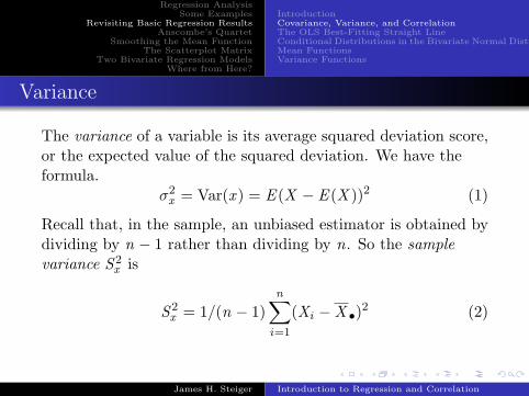
Variance
The variance of a variable is its average squared deviation score,or the expected value of the squared deviation. We have theformula.
σ2x = Var(x ) = E (X − E (X ))2 (1)
Recall that, in the sample, an unbiased estimator is obtained bydividing by n − 1 rather than dividing by n. So the samplevariance S 2
x is
S 2x = 1/(n − 1)
n∑i=1
(Xi −X •)2 (2)
James H. Steiger Introduction to Regression and Correlation

Regression AnalysisSome Examples
Revisiting Basic Regression ResultsAnscombe’s Quartet
Smoothing the Mean FunctionThe Scatterplot Matrix
Two Bivariate Regression ModelsWhere from Here?
IntroductionCovariance, Variance, and CorrelationThe OLS Best-Fitting Straight LineConditional Distributions in the Bivariate Normal DistributionMean FunctionsVariance Functions
Covariance
The covariance of a two variables is the average cross-productof their deviation scores, or the expected value of the product oftheir deviations. We have the formula.
σxy = Cov(x , y) = E (X − E (X ))(Y − E (Y )) (3)
The sample covariance Sxy is
Sxy = 1/(n − 1)n∑
i=1
(Xi −X •)(Yi −Y •) (4)
James H. Steiger Introduction to Regression and Correlation

Regression AnalysisSome Examples
Revisiting Basic Regression ResultsAnscombe’s Quartet
Smoothing the Mean FunctionThe Scatterplot Matrix
Two Bivariate Regression ModelsWhere from Here?
IntroductionCovariance, Variance, and CorrelationThe OLS Best-Fitting Straight LineConditional Distributions in the Bivariate Normal DistributionMean FunctionsVariance Functions
Correlation
The correlation ρxy between two variables is the averagecross-product of their standard scores, or
ρxy = E (ZxZy) =σxy
σxσy(5)
James H. Steiger Introduction to Regression and Correlation

Regression AnalysisSome Examples
Revisiting Basic Regression ResultsAnscombe’s Quartet
Smoothing the Mean FunctionThe Scatterplot Matrix
Two Bivariate Regression ModelsWhere from Here?
IntroductionCovariance, Variance, and CorrelationThe OLS Best-Fitting Straight LineConditional Distributions in the Bivariate Normal DistributionMean FunctionsVariance Functions
The OLS Best-Fitting Straight Line
The Ordinary Least Squares line of best fit to a data set is theline that minimizes the sum of squared residuals in the up-down(Y ) direction. Using some straightforward calculus, we canprove that this line has a slope ofβ1 = ρyxσy/σx = σyx/σ
2x = σyxσ
−1xx and an intercept of
β0 = µy − β1µx , with corresponding (non-Greek) formulas inthe sample.
With modern software like R, of course we will never have tocompute any of these quantities, unless it is for fun.
However, our predicted scores are of the form
Y = β1X + β0 (6)
James H. Steiger Introduction to Regression and Correlation

Regression AnalysisSome Examples
Revisiting Basic Regression ResultsAnscombe’s Quartet
Smoothing the Mean FunctionThe Scatterplot Matrix
Two Bivariate Regression ModelsWhere from Here?
IntroductionCovariance, Variance, and CorrelationThe OLS Best-Fitting Straight LineConditional Distributions in the Bivariate Normal DistributionMean FunctionsVariance Functions
Conditional Distributions — The Mean
When Y and X have a bivariate normal distribution, theconditional distribution of Y given X is normal, with aconditional mean that follows the OLS linear regression rule,that is
E (Y |X = x ) = β0 + β1x (7)
where β1 and β0 are the slope and intercept of the OLSregression line.
James H. Steiger Introduction to Regression and Correlation

Regression AnalysisSome Examples
Revisiting Basic Regression ResultsAnscombe’s Quartet
Smoothing the Mean FunctionThe Scatterplot Matrix
Two Bivariate Regression ModelsWhere from Here?
IntroductionCovariance, Variance, and CorrelationThe OLS Best-Fitting Straight LineConditional Distributions in the Bivariate Normal DistributionMean FunctionsVariance Functions
Conditional Distributions – The Variance
The conditional distribution of Y given X has a variance thatis constant, specifically,
Var(Y |X = x ) = σ2ε = (1− ρ2
xy)σ2y (8)
James H. Steiger Introduction to Regression and Correlation

Regression AnalysisSome Examples
Revisiting Basic Regression ResultsAnscombe’s Quartet
Smoothing the Mean FunctionThe Scatterplot Matrix
Two Bivariate Regression ModelsWhere from Here?
IntroductionCovariance, Variance, and CorrelationThe OLS Best-Fitting Straight LineConditional Distributions in the Bivariate Normal DistributionMean FunctionsVariance Functions
Conditional Distribution of Heights
Weisberg discusses the conditional distribution ideas wereviewed above in Section 1.2–1.3 of ALR. The ”MeanFunction” that gives the conditional mean of Y given X issimply the OLS regression line.
James H. Steiger Introduction to Regression and Correlation

Regression AnalysisSome Examples
Revisiting Basic Regression ResultsAnscombe’s Quartet
Smoothing the Mean FunctionThe Scatterplot Matrix
Two Bivariate Regression ModelsWhere from Here?
IntroductionCovariance, Variance, and CorrelationThe OLS Best-Fitting Straight LineConditional Distributions in the Bivariate Normal DistributionMean FunctionsVariance Functions
Mean Function
In Figure 1.8, Weisberg presents the conditional mean lineestimated by the OLS regression line, and contrasts it withan “identity” line that represents daughters having, onaverage, the same height as their mothers.By contrasting the two lines, you can see that daughters oftall mothers tend to be taller than average, but somewhatshorter than their mothers.Likewise, daughters of short mothers tend to be shorterthan the average woman, but taller than their mothers.This is the well-known phenomenon of “regression towardthe mean” discussed in detail in Psychology 310.
James H. Steiger Introduction to Regression and Correlation

Regression AnalysisSome Examples
Revisiting Basic Regression ResultsAnscombe’s Quartet
Smoothing the Mean FunctionThe Scatterplot Matrix
Two Bivariate Regression ModelsWhere from Here?
IntroductionCovariance, Variance, and CorrelationThe OLS Best-Fitting Straight LineConditional Distributions in the Bivariate Normal DistributionMean FunctionsVariance Functions
Regression Toward the Mean
> ## Scatterplot Mheight on horizontal,> ## Dheight on vertical> ## In an L-shaped box> ## Smaller than normal points> ## Point character is a bullet> plot(Mheight,Dheight,bty="l",cex=.3,pch=20)> ## Next draw line with b0=0> ## b1=1 dotted red> abline(0,1,lty=2,col="red")> ## Next draw regression line> ## Dheight~Mheight solid blue> abline(lm(Dheight~Mheight),lty=1,col="blue")
James H. Steiger Introduction to Regression and Correlation

Regression AnalysisSome Examples
Revisiting Basic Regression ResultsAnscombe’s Quartet
Smoothing the Mean FunctionThe Scatterplot Matrix
Two Bivariate Regression ModelsWhere from Here?
IntroductionCovariance, Variance, and CorrelationThe OLS Best-Fitting Straight LineConditional Distributions in the Bivariate Normal DistributionMean FunctionsVariance Functions
Regression Toward the Mean
●
●
●
●
●
●
●
●
●
●
●
●
●
●
●
● ●
●
●
●
●
●
●
●
●●
●
●
●
●
●
●
●
●
●
●
●●
●●
● ●
●
●
●
●
●
●
●
●
●
●
●
●
●
●
● ●
●
●
●
● ●
●
●
●
●
●
●
●
●
●●
●
●
●
●
●
●
●
●
●
●
●
● ●
●
●
●●
●
●
●
●
●
●
●
●
●
●
●
●
●
●
●
●
●
●
●
●
●●
●
●
●
●
●
●
●
●
●● ●
●
●
●●
●
●
●
●
●
●
●
●
●
●
●
●
●
●
●
●
●●
●
●
●
●
●●
●
●
●
●
●
●
●
●
●
●
● ●●
●
●
●
● ●
●
●
●
●
●
●
●
●
●
●
●
●
●
●
●
●
●
●
●
●
●
●
●
●
●
●
●
●
●
●
●
●
●
●
●
●
●
●
●
●
●
●
●
●
●
●
●
●
●
●
●●
●
●
●
●
●
●
●
●
●
●
●
●
●●
●
●
●
●
●
●
●
●
●
●
●
●
●
●
●
●
●
●
●
●
●
●
●
●
●
●
●
●
●
●
●
●
●
●
●
●
●
● ●
●
●
●
●
●
●
●
●
●
●
●
●
●
●
●
●
●
●
●
●
●
●
●
●
●
●
●
●
●
●
●
●
●
●
●
●
●
●
●
●
●
●
●
●
●●
●
●
●
●● ●
●
●
●
●
●
●
●
●
●
●
●
●
●
●
●
●
● ●
●
●
●
●
●
●
●
●
●
●
●
●
●
●
●
●●
●
●
●
●
●
●
●
●
●
● ● ● ●
●
●
●
●● ●
●
●
●
●
●
● ●
●
●
●
●
●
●
●
●
●
●
●●
●
●
●
●
●
● ●
●
●
●●
●
●
●
●
●
●
●
●
●
● ●
●
●
●
●
●
●
●●
●
●
●
●
●
●
●
●●
●
●
●
●
●
●
●
●
●
●
●
●
●
●
●
●
●
●
●
●
●
●
●
●
●
●
●
●
●●
●
●
●
●
●
●
●
● ●
●
●
●
●
●
●
●
● ●
●
●
● ●
● ●
●
●
●
●● ●
●●
●
●
●
●
●
●
●
●
●
●
●
●
●
●
●
●
●●
●
●
●
● ●
●
●
●
●
●
● ●
●
●
●
●
●
●
●
●
●
●
●
●
●
●
●
●
●
●
●
●
●
●
●
●
●
●
●
●
●
●
●
●
●
●
●
●
●
● ●
●
●
●
●
●
●
●
●
●
●
●
●
●
●
●●
●
●
●
●
●
● ●
●
●
●
●
●
●
●
●
●
●
●
● ●
●
●
●
●
●
●
●
●
●
●
●
●
●
●
●
●
●
●
●
●
●
●
●
●
●
●
●
●
●
●●
●
●
●
●
●
●
●
●
●
●
●●
●
●
● ●
●
●
●
●
● ●
●
●
●
●
●
●
●
●
●
●
●
●
●
●
● ●
●
● ● ●
●
●
●
●
●
●
●
●
●
●
●
●
●
●
●
● ●
●
●
●
●
●
●
●
●
●
●
●
●
●
●
●
●
●
●
●
●
●
●
●
●
●
●
●
●
●
●
●
●
●
●
●●
●
●
●
●
●
●
●
●
●
●
●
●
●
●
●
●
●
●
●
●
●
●●
●
●
●
●
●
●
●
●
●
●
●
●
●
●
●
●
●
●
●
●
● ●
●
●
●
●
●
●
●
●
●
●●
●
●
●
●
● ●
●
●
●
●
●
●
●
●
●●
●
●
●
●
●
●
●
●
●
●
●
●
●●
●
●
●
●●
●
●
●
●
●
●
●●
●
●
●
●
●
●
●
●
●●
●
●
●
●
●
●
●
●●
●●
●
●
●
●
●
●
●
●
●
●
●
●
●
●
●
●
●
●
●
●
● ●
●
●
● ●
●●
●
● ●
●
●
●●
●
●
●
●
●
●
●
●
●
●
●
●
●
●
●
●
●
●
●
●
●
●
●●
●
●
●
●
●
●
●
●
●
●
●
●
●
● ●
●
●
●
●
●
●
●
● ●
●
●
●
●
●
●
●
●
●
●
●
●
●
●●
●●
●
●
●
●
●
●
●
●
●●
●
●
●
●
●
●
●
●
●
● ●
●
●
●
●
●
●
●
●
●
●
●
●
●
●
●
●
●
●
●
●
●
●
●
●
●
●
●
●
●
●
●
●
●
●
●
●
● ●
● ●
●
●
● ●
●
●●
●
●
●
●
●
●
●
●
●
●
●
●
●
●●
●
●
●
●
● ●
●
●
●
●
●
●
●
●
●
●
●
● ●
●
●
●
●
●
●
●
●
●
●
●
●●
●
●
●
●
●
●
●
●
●
●
●
●
●
●
●
●
●
●
●
●
●●
●
●
●
●
●
●
●
●
●
●
●
●
●
●
●
●
●
●
●
●
●
●
●
●
●
●
● ●
●
●
●
●
●
●
●
●
●
●
●
●
●
●●
●
●
●
●
●
●
●●
●
●
● ●
●
●
●
●
●
●
●
●
● ●
●
●
●●
●
●
●
●
●
●
●
●
●
●
●
●
●
●
●
●
●●
●
●
●
●
●
●
●
●
●
●
●
●
●
●
●
●
●
●
●
●
●
●
●
●
●
●
●
●
●
●
●
●
●
●
●
●●●
●
●
●
●
●
●●
●
●
●
●
●
●
●
●
● ●
●
●
●
●
●
●
●
●
●
●
●
●
●
●
●
●
●
● ●
●
●
●
●
●
●
●
●
●
●
●
●
●
●
●
●
●
●
●
●
●
●
●
●
● ●
●
●
●
●
●
●
●●
●
●
● ●
●
●
●
●
●●
●
● ●
●
●
●
● ●
●
●
● ●
●
●
●
●
●
●
●
●
●
●●
●●
●
●
●
●
●
●
●
● ●
● ●
●
●
●
●
●
●
●
●
●
●
●
●
●
●
●
●
●
●
●
●
●
●
●
●
●
●
●
●
●
● ●
●
●
●
●
●
●
●
●
●
●
●
●
●
●
●
55 60 65 70
5560
6570
Mheight
Dhe
ight
James H. Steiger Introduction to Regression and Correlation

Regression AnalysisSome Examples
Revisiting Basic Regression ResultsAnscombe’s Quartet
Smoothing the Mean FunctionThe Scatterplot Matrix
Two Bivariate Regression ModelsWhere from Here?
IntroductionCovariance, Variance, and CorrelationThe OLS Best-Fitting Straight LineConditional Distributions in the Bivariate Normal DistributionMean FunctionsVariance Functions
Nonlinear Mean Functions
Depending on the type of data and the nature of therelationship between X and Y , the conditional mean functionneed not be linear. We’ll have a lot more to say about that.
James H. Steiger Introduction to Regression and Correlation

Regression AnalysisSome Examples
Revisiting Basic Regression ResultsAnscombe’s Quartet
Smoothing the Mean FunctionThe Scatterplot Matrix
Two Bivariate Regression ModelsWhere from Here?
IntroductionCovariance, Variance, and CorrelationThe OLS Best-Fitting Straight LineConditional Distributions in the Bivariate Normal DistributionMean FunctionsVariance Functions
Variance Functions
A frequent assumption in fitting linear regression models is thatthe variance function is the same for every value of X . This isusually written as
Var(Y |X = x ) = σ2 (9)
where σ2 is a generally unknown positive constant.
However, we’ll also deal with a variety of situations where thevariance function is non-constant.
James H. Steiger Introduction to Regression and Correlation

Regression AnalysisSome Examples
Revisiting Basic Regression ResultsAnscombe’s Quartet
Smoothing the Mean FunctionThe Scatterplot Matrix
Two Bivariate Regression ModelsWhere from Here?
Anscombe’s Quartet
It is essential to always examine the scatterplot for bivariatedata. The same summary statistics and regression coefficients(means, variances, covariances, correlation, b0, b1) can yieldvery different scatterplots.
Anscombe (1973) dramatized this phenomenon with 4 smalldata sets that have come to be known as “Anscombe’s Quartet.”
They are plotted on the next slide. What do we see (C.P.)?
James H. Steiger Introduction to Regression and Correlation

Regression AnalysisSome Examples
Revisiting Basic Regression ResultsAnscombe’s Quartet
Smoothing the Mean FunctionThe Scatterplot Matrix
Two Bivariate Regression ModelsWhere from Here?
Anscombe’s Quartet
> par(mfrow=c(2,2))> data(anscombe)> attach(anscombe)> plot(x1,y1,xlim=c(4,20),ylim=c(3,13))> abline(lm(y1~x1),col="red")> plot(x2,y2,xlim=c(4,20),ylim=c(3,13))> abline(lm(y2~x2),col="red")> plot(x3,y3,xlim=c(4,20),ylim=c(3,13))> abline(lm(y3~x3),col="red")> plot(x4,y4,xlim=c(4,20),ylim=c(3,13))> abline(lm(y4~x4,col="red"))
James H. Steiger Introduction to Regression and Correlation
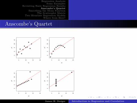
Regression AnalysisSome Examples
Revisiting Basic Regression ResultsAnscombe’s Quartet
Smoothing the Mean FunctionThe Scatterplot Matrix
Two Bivariate Regression ModelsWhere from Here?
Anscombe’s Quartet
●
●
●
●
●
●
●
●
●
●
●
5 10 15 20
46
810
12
x1
y1
●
●
●●
●
●
●
●
●
●
●
5 10 15 20
46
810
12
x2
y2
●
●
●
●
●
●
●
●
●
●
●
5 10 15 20
46
810
12
x3
y3
●
●
●
●●
●
●
●
●
●
●
5 10 15 20
46
810
12
x4
y4
James H. Steiger Introduction to Regression and Correlation

Regression AnalysisSome Examples
Revisiting Basic Regression ResultsAnscombe’s Quartet
Smoothing the Mean FunctionThe Scatterplot Matrix
Two Bivariate Regression ModelsWhere from Here?
The Loess Smoother
We can estimate the mean function with a model, as we havedone with linear regression assuming bivariate normality.
However, we can also “let the data speak for themselves” withvarious nonparametric techniques. One approach is smoothing.The loess smoother:
1 Steps across the plot and, for each value x of X , gathers allthe points within a certain span of x .
2 A regression line is fit to these data (not, in general, bysimple linear regression!), and then
3 The conditional mean at x is calculated from thatregression line.
4 The points resulting from this process are then graphed asa continuous line.
The original acronym LOWESS (LOcally WEighted ScatterplotSmoothing) is now often spelled as “loess.”
James H. Steiger Introduction to Regression and Correlation

Regression AnalysisSome Examples
Revisiting Basic Regression ResultsAnscombe’s Quartet
Smoothing the Mean FunctionThe Scatterplot Matrix
Two Bivariate Regression ModelsWhere from Here?
The Loess Smoother
R automates the calculation and plotting of the loess smoother.Here is some code to generate a smoothed line for the heightsdata.
> plot(Dheight~Mheight,cex=.1,pch=20,bty="l")> abline(lm(Dheight~Mheight),lty=1)> lines(lowess(Dheight~Mheight,f=6/10,iter=1),lty=2)> legend("bottomright", c("OLS", "loess"),+ lty = c(1, 2),col=c("blue","red"))
James H. Steiger Introduction to Regression and Correlation

Regression AnalysisSome Examples
Revisiting Basic Regression ResultsAnscombe’s Quartet
Smoothing the Mean FunctionThe Scatterplot Matrix
Two Bivariate Regression ModelsWhere from Here?
The Loess Smoother
●
●
●
●
●
●
●
●
●
●
●
●
●
●
●
● ●
●
●
●
●
●
●
●
●●
●
●
●
●
●
●
●
●
●
●
●●
●●
● ●
●
●
●
●
●
●
●
●
●
●
●
●
●
●
● ●
●
●
●
● ●
●
●
●
●
●
●
●
●
●●
●
●
●
●
●
●
●
●
●
●
●
● ●
●
●
●●
●
●
●
●
●
●
●
●
●
●
●
●
●
●
●
●
●
●
●
●
●●
●
●
●
●
●
●
●
●
●● ●
●
●
●●
●
●
●
●
●
●
●
●
●
●
●
●
●
●
●
●
●●
●
●
●
●
●●
●
●
●
●
●
●
●
●
●
●
● ●●
●
●
●
● ●
●
●
●
●
●
●
●
●
●
●
●
●
●
●
●
●
●
●
●
●
●
●
●
●
●
●
●
●
●
●
●
●
●
●
●
●
●
●
●
●
●
●
●
●
●
●
●
●
●
●
●●
●
●
●
●
●
●
●
●
●
●
●
●
●●
●
●
●
●
●
●
●
●
●
●
●
●
●
●
●
●
●
●
●
●
●
●
●
●
●
●
●
●
●
●
●
●
●
●
●
●
●
● ●
●
●
●
●
●
●
●
●
●
●
●
●
●
●
●
●
●
●
●
●
●
●
●
●
●
●
●
●
●
●
●
●
●
●
●
●
●
●
●
●
●
●
●
●
●●
●
●
●
●● ●
●
●
●
●
●
●
●
●
●
●
●
●
●
●
●
●
● ●
●
●
●
●
●
●
●
●
●
●
●
●
●
●
●
●●
●
●
●
●
●
●
●
●
●
● ● ● ●
●
●
●
●● ●
●
●
●
●
●
● ●
●
●
●
●
●
●
●
●
●
●
●●
●
●
●
●
●
● ●
●
●
●●
●
●
●
●
●
●
●
●
●
● ●
●
●
●
●
●
●
●●
●
●
●
●
●
●
●
●●
●
●
●
●
●
●
●
●
●
●
●
●
●
●
●
●
●
●
●
●
●
●
●
●
●
●
●
●
●●
●
●
●
●
●
●
●
● ●
●
●
●
●
●
●
●
● ●
●
●
● ●
● ●
●
●
●
●● ●
●●
●
●
●
●
●
●
●
●
●
●
●
●
●
●
●
●
●●
●
●
●
● ●
●
●
●
●
●
● ●
●
●
●
●
●
●
●
●
●
●
●
●
●
●
●
●
●
●
●
●
●
●
●
●
●
●
●
●
●
●
●
●
●
●
●
●
●
● ●
●
●
●
●
●
●
●
●
●
●
●
●
●
●
●●
●
●
●
●
●
● ●
●
●
●
●
●
●
●
●
●
●
●
● ●
●
●
●
●
●
●
●
●
●
●
●
●
●
●
●
●
●
●
●
●
●
●
●
●
●
●
●
●
●
●●
●
●
●
●
●
●
●
●
●
●
●●
●
●
● ●
●
●
●
●
● ●
●
●
●
●
●
●
●
●
●
●
●
●
●
●
● ●
●
● ● ●
●
●
●
●
●
●
●
●
●
●
●
●
●
●
●
● ●
●
●
●
●
●
●
●
●
●
●
●
●
●
●
●
●
●
●
●
●
●
●
●
●
●
●
●
●
●
●
●
●
●
●
●●
●
●
●
●
●
●
●
●
●
●
●
●
●
●
●
●
●
●
●
●
●
●●
●
●
●
●
●
●
●
●
●
●
●
●
●
●
●
●
●
●
●
●
● ●
●
●
●
●
●
●
●
●
●
●●
●
●
●
●
● ●
●
●
●
●
●
●
●
●
●●
●
●
●
●
●
●
●
●
●
●
●
●
●●
●
●
●
●●
●
●
●
●
●
●
●●
●
●
●
●
●
●
●
●
●●
●
●
●
●
●
●
●
●●
●●
●
●
●
●
●
●
●
●
●
●
●
●
●
●
●
●
●
●
●
●
● ●
●
●
● ●
●●
●
● ●
●
●
●●
●
●
●
●
●
●
●
●
●
●
●
●
●
●
●
●
●
●
●
●
●
●
●●
●
●
●
●
●
●
●
●
●
●
●
●
●
● ●
●
●
●
●
●
●
●
● ●
●
●
●
●
●
●
●
●
●
●
●
●
●
●●
●●
●
●
●
●
●
●
●
●
●●
●
●
●
●
●
●
●
●
●
● ●
●
●
●
●
●
●
●
●
●
●
●
●
●
●
●
●
●
●
●
●
●
●
●
●
●
●
●
●
●
●
●
●
●
●
●
●
● ●
● ●
●
●
● ●
●
●●
●
●
●
●
●
●
●
●
●
●
●
●
●
●●
●
●
●
●
● ●
●
●
●
●
●
●
●
●
●
●
●
● ●
●
●
●
●
●
●
●
●
●
●
●
●●
●
●
●
●
●
●
●
●
●
●
●
●
●
●
●
●
●
●
●
●
●●
●
●
●
●
●
●
●
●
●
●
●
●
●
●
●
●
●
●
●
●
●
●
●
●
●
●
● ●
●
●
●
●
●
●
●
●
●
●
●
●
●
●●
●
●
●
●
●
●
●●
●
●
● ●
●
●
●
●
●
●
●
●
● ●
●
●
●●
●
●
●
●
●
●
●
●
●
●
●
●
●
●
●
●
●●
●
●
●
●
●
●
●
●
●
●
●
●
●
●
●
●
●
●
●
●
●
●
●
●
●
●
●
●
●
●
●
●
●
●
●
●●●
●
●
●
●
●
●●
●
●
●
●
●
●
●
●
● ●
●
●
●
●
●
●
●
●
●
●
●
●
●
●
●
●
●
● ●
●
●
●
●
●
●
●
●
●
●
●
●
●
●
●
●
●
●
●
●
●
●
●
●
● ●
●
●
●
●
●
●
●●
●
●
● ●
●
●
●
●
●●
●
● ●
●
●
●
● ●
●
●
● ●
●
●
●
●
●
●
●
●
●
●●
●●
●
●
●
●
●
●
●
● ●
● ●
●
●
●
●
●
●
●
●
●
●
●
●
●
●
●
●
●
●
●
●
●
●
●
●
●
●
●
●
●
● ●
●
●
●
●
●
●
●
●
●
●
●
●
●
●
●
55 60 65 70
5560
6570
Mheight
Dhe
ight
OLSloess
James H. Steiger Introduction to Regression and Correlation

Regression AnalysisSome Examples
Revisiting Basic Regression ResultsAnscombe’s Quartet
Smoothing the Mean FunctionThe Scatterplot Matrix
Two Bivariate Regression ModelsWhere from Here?
The Scatterplot Matrix
When we have several potential predictors, a scatterplotmatrix can help us immediately spot which predictors havean exploitable relationship with the criterion, andAlso make it relatively easy to spot categorical variablesand outliers
Section 1.6 of ALR discusses construction of a scatterplotmatrix for data from an analysis of fuel consumption in theU.S.. Let’s load the data
> data(fuel2001)> attach(fuel2001)
and take a quick look.
> edit(data)
James H. Steiger Introduction to Regression and Correlation

Regression AnalysisSome Examples
Revisiting Basic Regression ResultsAnscombe’s Quartet
Smoothing the Mean FunctionThe Scatterplot Matrix
Two Bivariate Regression ModelsWhere from Here?
Variable Definitions
James H. Steiger Introduction to Regression and Correlation

Regression AnalysisSome Examples
Revisiting Basic Regression ResultsAnscombe’s Quartet
Smoothing the Mean FunctionThe Scatterplot Matrix
Two Bivariate Regression ModelsWhere from Here?
Additional Calculated Variables
Both Drivers and FuelC are state totals, so these will be largerin states with more people and smaller in less populous states.Income is computed per person. To make all these comparableand to attempt to eliminate the effect of size of the state, we:
Compute rates Dlic = Drivers/Pop andFuel = FuelC/Pop, and rescale Income to be in thousands.Also replace Miles by its (base-two) logarithm before doingany further analysis. (Justification for replacing Miles withlog(Miles) is deferred to ALR Problem 7.7.)
> fuel2001$Dlic <- 1000*fuel2001$Drivers/fuel2001$Pop> fuel2001$Fuel <- 1000*fuel2001$FuelC/fuel2001$Pop> fuel2001$Income <- fuel2001$Income/1000> fuel2001$logMiles <- logb(fuel2001$Miles,2)> names(fuel2001)
[1] "Drivers" "FuelC" "Income" "Miles" "MPC" "Pop"[7] "Tax" "State" "Dlic" "Fuel" "logMiles"
James H. Steiger Introduction to Regression and Correlation
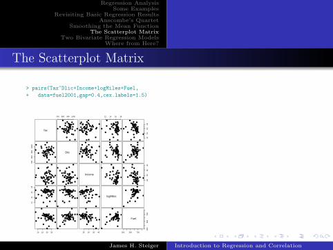
Regression AnalysisSome Examples
Revisiting Basic Regression ResultsAnscombe’s Quartet
Smoothing the Mean FunctionThe Scatterplot Matrix
Two Bivariate Regression ModelsWhere from Here?
The Scatterplot Matrix
> pairs(Tax~Dlic+Income+logMiles+Fuel,+ data=fuel2001,gap=0.4,cex.labels=1.5)
Tax
700 800 900 1000
●
●
●
●
●
●
●
●
●
●
●
●
●
●
●
●●
●
●
●
●
●
●●
●●
●
●●
●
●
●
●
●
●●
●
●
●
●
●
●
●●
●
●
●
●
●
●
●
●
●
●
●
●
●
●
●
●
●
●
●
●
●
●
●●
●
●
●
●
●
●●
●●
●
● ●
●
●
●
●
●
●●
●
●
●
●
●
●
● ●
●
●
●
●
●
●
●
12 14 16 18
●
●
●
●
●
●
●
●
●
●
●
●
●
●
●
●●
●
●
●
●
●
●●
●●
●
●●
●
●
●
●
●
●●
●
●
●
●
●
●
● ●
●
●
●
●
●
●
●
1015
2025
●
●
●
●
●
●
●
●
●
●
●
●
●
●
●
●●
●
●
●
●
●
●●
●●
●
●●
●
●
●
●
●
●●
●
●
●
●
●
●
● ●
●
●
●
●
●
●
●
700
800
900
1000
●●
●
●
●
● ●
●
●
●
●
●
●
●
●●
●
●
●
●
●
●●
●
●
●
●●
●
●
●
●
●
●
●
●
●
●
●
●
●
●●
●
●
●
●
●
●●
●
Dlic
● ●
●
●
●
● ●
●
●
●
●
●
●
●
●●
●
●
●
●
●
●●
●
●
●
●●
●
●
●
●
●
●
●
●
●
●
●
●
●
●●
●
●
●
●
●
●●
●
●●
●
●
●
●●
●
●
●
●
●
●
●
●●
●
●
●
●
●
● ●
●
●
●
●●
●
●
●
●
●
●
●
●
●
●
●
●
●
●●
●
●
●
●
●
●●
●
●●
●
●
●
●●
●
●
●
●
●
●
●
●●
●
●
●
●
●
● ●
●
●
●
●●
●
●
●
●
●
●
●
●
●
●
●
●
●
●●
●
●
●
●
●
●●
●
●
●
●
●
●●
●
●
●
●● ●
●
●
● ●●
●●
●
●
●
●
●
●
●
●
●
●
●
●
●
●
●
●
●
●
●● ●
●
●●
●
●
●
● ●
●
●●
●
●
●
●
●●
●
●
●
●●●
●
●
●●●
●●
●
●
●
●
●
●
●
●
●
●
●
●
●
●
●
●
●
●
●●●
●
●●
●
●
●
● ●
●
●●
Income
●
●
●
●
●●
●
●
●
●●●
●
●
●●●
●●
●
●
●
●
●
●
●
●
●
●
●
●
●
●
●
●
●
●
●●●
●
●●
●
●
●
●●
●
●●
2530
3540
●
●
●
●
●●
●
●
●
● ●●
●
●
●●●
●●
●
●
●
●
●
●
●
●
●
●
●
●
●
●
●
●
●
●
●●●
●
●●
●
●
●
●●
●
●●
1214
1618
●
●
●
●
●
●
●
●
●
●●
●
●
●
●●
●
●●
●●
●
●●
●
●
●●
●
●
●
●
● ●●
●●
●
●
●
●●●
●
●
●
● ●
●
●
●
●
●
●
●
●
●
●
●
●
●●
●
●
●
●●
●
●●
●●
●
●●
●
●
●●
●
●
●
●
● ●●
●●
●
●
●
●●●
●
●
●
● ●
●
●
●
●
●
●
●
●
●
●
●
●
●●
●
●
●
●●
●
●●
●●
●
● ●
●
●
●●
●
●
●
●
●●●
●●
●
●
●
●●●
●
●
●
●●
●
●
● logMiles
●
●
●
●
●
●
●
●
●
● ●
●
●
●
●●
●
●●
●●
●
● ●
●
●
●●
●
●
●
●
● ●●
● ●
●
●
●
●●●
●
●
●
●●
●
●
●
10 15 20 25
●
●
●●
●
●
●
●
●
●
●
●
●
●
●●
●
●●
●●
●
●●●●
●
●●
●
●
●
●
●●
●
●
●
●
●
●●
●
●
●
●●
● ●●
●
●
●
●●
●
●
●
●
●
●
●
●
●
●
●●
●
●●
●●
●
●● ● ●
●
●●
●
●
●
●
●●
●
●
●
●
●
●●
●
●
●
●●
●●●
●
25 30 35 40
●
●
●●
●
●
●
●
●
●
●
●
●
●
●●
●
●●
●●
●
●●● ●
●
● ●
●
●
●
●
●●
●
●
●
●
●
●●
●
●
●
● ●
●●●
●
●
●
●●
●
●
●
●
●
●
●
●
●
●
●●
●
●●
●●
●
●●● ●
●
●●
●
●
●
●
●●
●
●
●
●
●
●●
●
●
●
● ●
●●●
●
300 500 700
300
500
700
Fuel
James H. Steiger Introduction to Regression and Correlation

Regression AnalysisSome Examples
Revisiting Basic Regression ResultsAnscombe’s Quartet
Smoothing the Mean FunctionThe Scatterplot Matrix
Two Bivariate Regression ModelsWhere from Here?
The Scatterplot Matrix
The row of the scatterplot matrix determines the variable thatis on the vertical axis, and the column of the scatterplot matrixdetermines the variable that is on the horizontal axis of anyscatterplot.
For example, the upper-right plot is in row 1 and column 5. Itshows a plot of Fuel on the vertical axis and Tax on thehorizontal axis.
James H. Steiger Introduction to Regression and Correlation

Regression AnalysisSome Examples
Revisiting Basic Regression ResultsAnscombe’s Quartet
Smoothing the Mean FunctionThe Scatterplot Matrix
Two Bivariate Regression ModelsWhere from Here?
Two Regression ModelsThe Bivariate Normal Model
In Psychology 310, we introduced least squares linearregression as a data analysis problem. We have these datapoints in the X −Y plane, and we wish to plot line thatcomes as close to the points as possible, in the least squaressense of minimizing the sum of squared residuals.Then, we pointed out that if X and Y are bivariate normal,the conditional distribution of Y given X is normal, withconditional mean function given by the regression line, andconstant conditional variance given by σ2
e .
James H. Steiger Introduction to Regression and Correlation

Regression AnalysisSome Examples
Revisiting Basic Regression ResultsAnscombe’s Quartet
Smoothing the Mean FunctionThe Scatterplot Matrix
Two Bivariate Regression ModelsWhere from Here?
Two Regression ModelsThe Fixed Regressors Model
Now we introduce a somewhat more general model.The X scores are considered fixed, and the Y scoresrandom.The conditional distribution of Y given X = x is normal,with constant variance σ2, and mean functionE (Y |X = x ) = β0 + β1x .
James H. Steiger Introduction to Regression and Correlation

Regression AnalysisSome Examples
Revisiting Basic Regression ResultsAnscombe’s Quartet
Smoothing the Mean FunctionThe Scatterplot Matrix
Two Bivariate Regression ModelsWhere from Here?
Where from Here?
If the data fall (pretty much) on a straight line, and theconditional variance is fairly constant, then the standardregression model will work well, and we can use its machineryfor computing estimates and (their) estimated standard errors.
However, if the model is inappropriate, as revealed in anonlinear function or inappropriate conditional variances, morework will be required. There are many possibilities that areinvestigated in detail in Psychology 313:
Fit a polynomial, as a special case of multiple regression.Transform the X and/or Y variables. An advantage of thisis that the machinery for gauging a transform iswell-established. There are also disadvantages.Try a different kind of model, like nonlinear regression or ageneralized linear model.
In this course, we will move quickly to multiple linear regressionand look at it briefly as an entree into more complex forms ofmultivariate analysis.
James H. Steiger Introduction to Regression and Correlation