The Step Decay Schedule: A Near Optimal, Geometrically Decaying Learning Rate Schedule

for Least Squares

Rong Ge*, Sham M. Kakade**, Rahul Kidambi*** and Praneeth Netrapalli****

* Duke University, Durham NC

** University of Washington Seattle WA

*** Cornell University, Ithaca NY

**** Microsoft Research India

Paper ID: 8546, NeurIPS 2019

SGD: Theory Vs. Practice

• Stochastic Gradient Descent (SGD) [Robbins & Monro, ‘51]• Simple to implement, drives modern Machine Learning applications.

• In theory [Ruppert ‘88, Polyak & Juditsky ‘92]• Relies on iterate averaging [Rakhlin et al. 2012, Bubeck 2014].• Employs polynomially decaying stepsizes.• Minimax optimal predictive guarantees.

• In practice [Bottou & Bousquet 2008]• Implementations predominantly use the final iterate of SGD.• Employs a geometrically decaying “step decay” schedule.• Strong computation vs. generalization tradeoffs.

This Paper: SGD’s Final Iterate For Least Squares

• Streaming Least Squares Regression – compute:

𝑤∗ ∈ argmin𝑤 𝑓 𝑤 = 12⋅E 𝑥,𝑦 ∼𝐷 𝑦 − 𝑤. 𝑥 2 ,

• Several recent works e.g. [Bach & Moulines 2013, Jain et al. 2016, 2017].

• Constant step size SGD + iterate averaging achieves minimax optimal rates.

• This paper: SGD’s final iterate behavior.

• Several works [Widrow et al. ‘60, Nagumo et al. ‘67, Proakis ‘74] etc.

• These efforts do not achieve minimax rates.

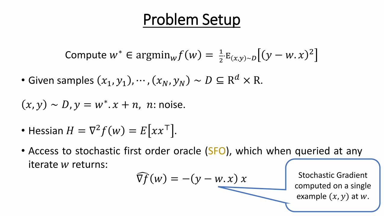
Problem Setup

Compute 𝑤∗ ∈ argmin𝑤𝑓 𝑤 = 1

2⋅E 𝑥,𝑦 ∼𝐷 𝑦 − 𝑤. 𝑥 2

• Given samples 𝑥1, 𝑦1 , ⋯ , 𝑥𝑁 , 𝑦𝑁 ∼ 𝐷 ⊆ R𝑑 × R.

𝑥, 𝑦 ∼ 𝐷, 𝑦 = 𝑤∗. 𝑥 + 𝑛, 𝑛: noise.

• Hessian 𝐻 = ∇2𝑓 𝑤 = 𝐸 𝑥𝑥⊤ .

• Access to stochastic first order oracle (SFO), which when queried at anyiterate 𝑤 returns:

∇𝑓 𝑤 = − 𝑦 − 𝑤. 𝑥 𝑥 Stochastic Gradient computed on a single example (𝑥, 𝑦) at 𝑤.

Problem Setup (2)

• Assumptions (for precise statements, refer to paper):

• A1. Strong convexity, i.e., 𝐻 ≻ 0 ⇒ 𝜇 = 𝜆𝑚𝑖𝑛 𝐻 > 0.

• A2. Bounded Inputs, i.e., ||𝑥||2 < R2 almost surely.

• Denote the condition number 𝜅 ≔ R2/𝜇.

• A3. Bounded noise, i.e., ∀ 𝑥, 𝑦 ∼ 𝐷, |𝑦 − 𝑤∗𝑥| < 𝜎 almost surely.

• Under A1-3, any algorithm outputting ෝ𝑤𝑡 with t-calls to an SFO [Vaart

2000] has error at least:

𝐹 ෝ𝑤𝑡 − 𝐹 𝑤∗ ≥𝑑𝜎2

𝑡.

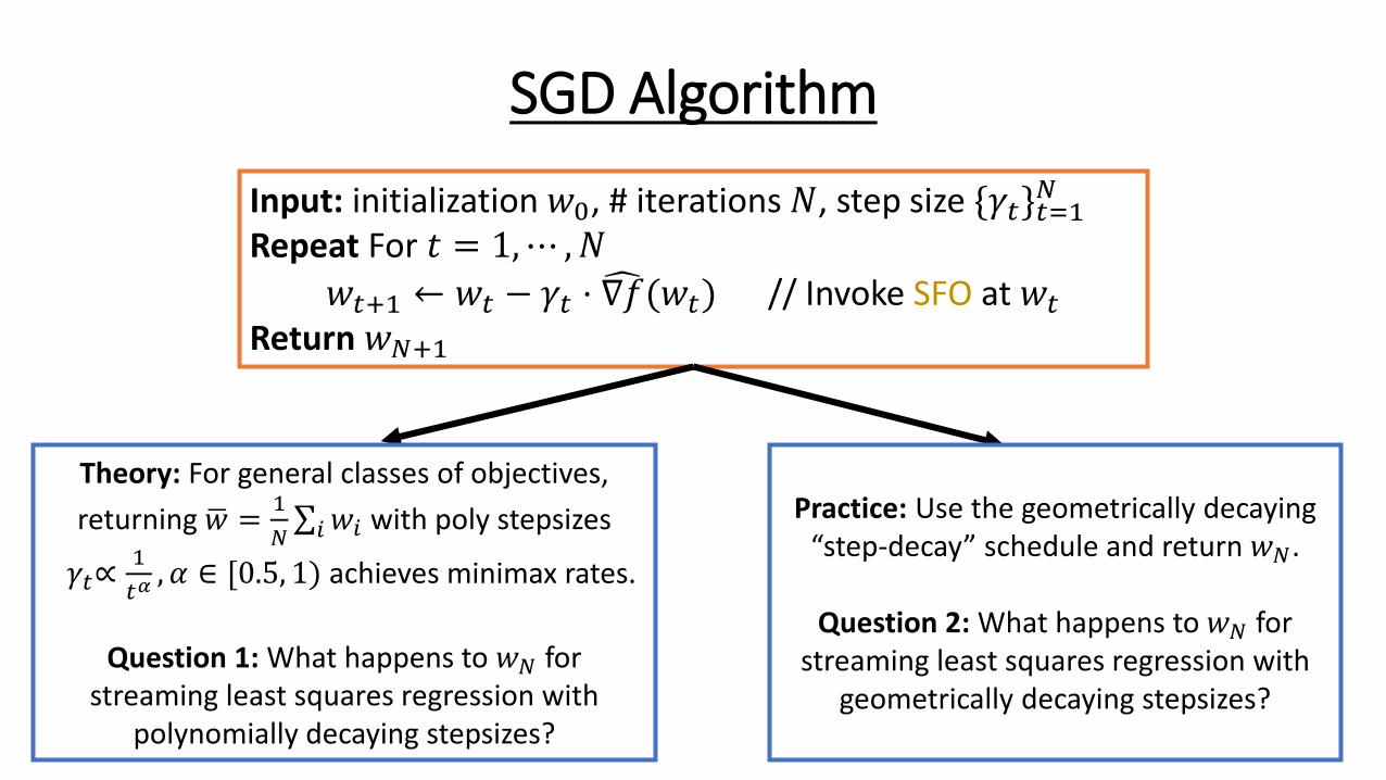
SGD Algorithm

Input: initialization 𝑤0, # iterations 𝑁, step size {𝛾𝑡}𝑡=1𝑁

Repeat For 𝑡 = 1,⋯ ,𝑁

𝑤𝑡+1 ← 𝑤𝑡 − 𝛾𝑡 ⋅ ∇𝑓(𝑤𝑡) // Invoke SFO at 𝑤𝑡

Return 𝑤𝑁+1

Theory: For general classes of objectives,

returning ഥ𝑤 =1

𝑁σ𝑖𝑤𝑖 with poly stepsizes

𝛾𝑡∝1

𝑡𝛼, 𝛼 ∈ [0.5, 1) achieves minimax rates.

Question 1: What happens to 𝑤𝑁 for streaming least squares regression with

polynomially decaying stepsizes?

Practice: Use the geometrically decaying “step-decay” schedule and return 𝑤𝑁.

Question 2: What happens to 𝑤𝑁 for streaming least squares regression with

geometrically decaying stepsizes?

Q1: SGD’s Final Iterate with Polynomially Decaying Stepsizes

Theorem (informal):For a given end time N, under assumptions A1-3, there exists a streaming least squares regression problem such that every step

size scheme 𝛾𝑡 =𝑎

𝑏+𝑡𝛼, with 𝛼 ∈ [0.5,1] suffers the error:

𝐸 𝐹 𝑤𝑁 − 𝐹 𝑤∗ ≥ 𝜅 ⋅𝑑𝜎2

𝑁.

Comments:

[1] Final iterate + poly decay: highly sub-optimal (by a condition number).

[2] Recall, iterate averaging + poly decay: optimal behavior.

SGD With The Step-Decay Schedule

• Remarks: Final iterate 𝑤 returned – similar to practice.• To run the algorithm: we require initial stepsize 𝛾0 and # iterations 𝑁.

• Used heavily in algorithms for modern ML/AI models [Krizhevsky et al. 2012].

Input: initialization 𝑤0, # iterations 𝑁, initial step size 𝛾0

Repeat for 𝑒 = 1,⋯ , log 𝑁:

𝛾𝑒 ← 𝛾0/2𝑒−1 // Halve learning rate every epoch

Repeat for 𝑡 = 1,⋯ ,𝑁/log 𝑁:

𝑤 ← 𝑤 − 𝛾𝑒 ⋅ ∇𝑓(𝑤) // Invoke SFO at 𝑤Return 𝑤

Q2: SGD’s Final Iterate with Step-Decay Schedule

• Variance term: Near-optimal rate (upto log 𝑁 ) factors.

• SGD with step-decay requires knowing # iterations N in advance.

• Significant difference compared to polynomially decaying stepsizes.

• Related work: Shamir & Zhang (2012), Jain, Nagaraj & Netrapalli (2019).

Theorem (informal):

Under assumptions A1-3, SGD with an initial learning rate 𝛾 =1

R2and the

step decay schedule offers the following guarantee:

𝐸 𝐹 𝑤 − 𝐹 𝑤∗ ≤ exp −𝑁

𝜅 ⋅ log 𝑁⋅ 𝐹 𝑤0 − 𝐹 𝑤∗ + log 𝑁 ⋅

𝑑𝜎2

𝑁.

Simulations: Synthetic Streaming Least Squares

• Plot of final iterate’s error (y-axis) against condition number (x-axis)

Polynomially Decaying Stepsizes: Error grows linearly

wrt Condition Number.

Step Decay: Error is near constant as a function of condition number

(sub-optimal by log(𝑇) factors)

Non-Convex Optimization: CIFAR-10 With ResNet-44

• Grid search three schemes (with a fixed end time):

(a) 𝜂𝑡 =𝜂0

1+𝑏⋅𝑡, (b) 𝜂𝑡 =

𝜂0

1+𝑏 𝑡, (c) 𝜂𝑡 = 𝜂0 ⋅ exp(−𝑏𝑡)

11.6%

10.2%

7.6%

Towards Anytime Algorithms

• This paper’s results: assumes the # iterations 𝑁 to be fixed apriori.

• How about anytime algorithms?

• Anytime ⇒ Doesn’t require knowing # iterations N in advance.

• Iterate averaging + polynomially decaying stepsizes ⇒ anytime optimal.

• What about the final iterate?

• The next slide presents anytime behavior of SGD’s final iterate for thestreaming least squares regression problem.

Q2: SGD’s Final Iterate with Step-Decay Schedule

• Related work: See Harvey et al. (2019) for a similar statement in non-

smooth stochastic convex optimization.

• See also the related work of Ge et al. (2019), a COLT open problem about

understanding the sub-optimality of query points more generally.

Theorem (informal):

Under assumptions A1-3, SGD’s final iterate with stepsizes 𝛾𝑡 ≤ 1/(2 R2)queries highly sub-optimal iterates infinitely often. In particular,

limsup𝑇→∞

𝐸 𝑓 𝑤𝑇 − 𝑓(𝑤∗)

𝑑𝜎2/𝑇≥ 𝐶 ⋅

𝜅

log 𝜅

Other Empirical Results on CIFAR-10 with ResNet-44

• Suffix iterate averaging versus final iterate with polynomiallydecaying stepsizes:• Empirical evidence indicates that suffix averaging (regardless of the suffix

length) offers little advantage over the final iterate behavior for non-convexoptimization involving training a ResNet-44 model on CIFAR-10 dataset.

• Hyper-parameter optimization with truncated runs:• The broader issues concerning design of anytime optimal SGD methods tends

to imply hyper-parameter search methods based on truncated runs maybenefit from a round of rethinking.

Conclusions

• For the streaming least squares problem, SGD’s final iterate behavior:• With polynomially decaying stepsizes is highly sub-optimal.

• With step-decay schedule is near-optimal (upto logarithmic factors).

• The behavior of SGD’s final iterate in an anytime sense is sub-optimalin that SGD needs to query highly sub-optimal points infinitely often.

• Empirical results and ramifications towards the use of iterateaveraging and for hyper-parameter optimization is shown throughoptimizing a ResNet-44 on the CIFAR-10 dataset.