The Stability of an Inverted Pendulum

Mentor: John Gemmer

Sean Ashley

Avery Hope D’Amelio Jiaying Liu

Cameron Warren Abstract: The inverted pendulum is a simple system in which both stable and unstable state are easily observed. The upward inverted state is unstable, though it has long been known that a simple rigid pendulum can be stabilized in its inverted state by oscillating its base at an angle. We made the model to simulate the stabilization of the simple inverted pendulum. Also, the numerical analysis was used to find the stability angle.

Introduction

The model of the simple pendulum problem is one the most well studied dynamical systems.

Imagine a weight attached to the end of weightless rod that is freely swinging back and forth about some

pivot without friction. The governing equation for this idealized mathematical model is given as  

€

d2θdt 2

+ glsinθ = 0 , where

€

g   is gravitational acceleration, 𝑙 is the length of the pendulum, and 𝜃 is the

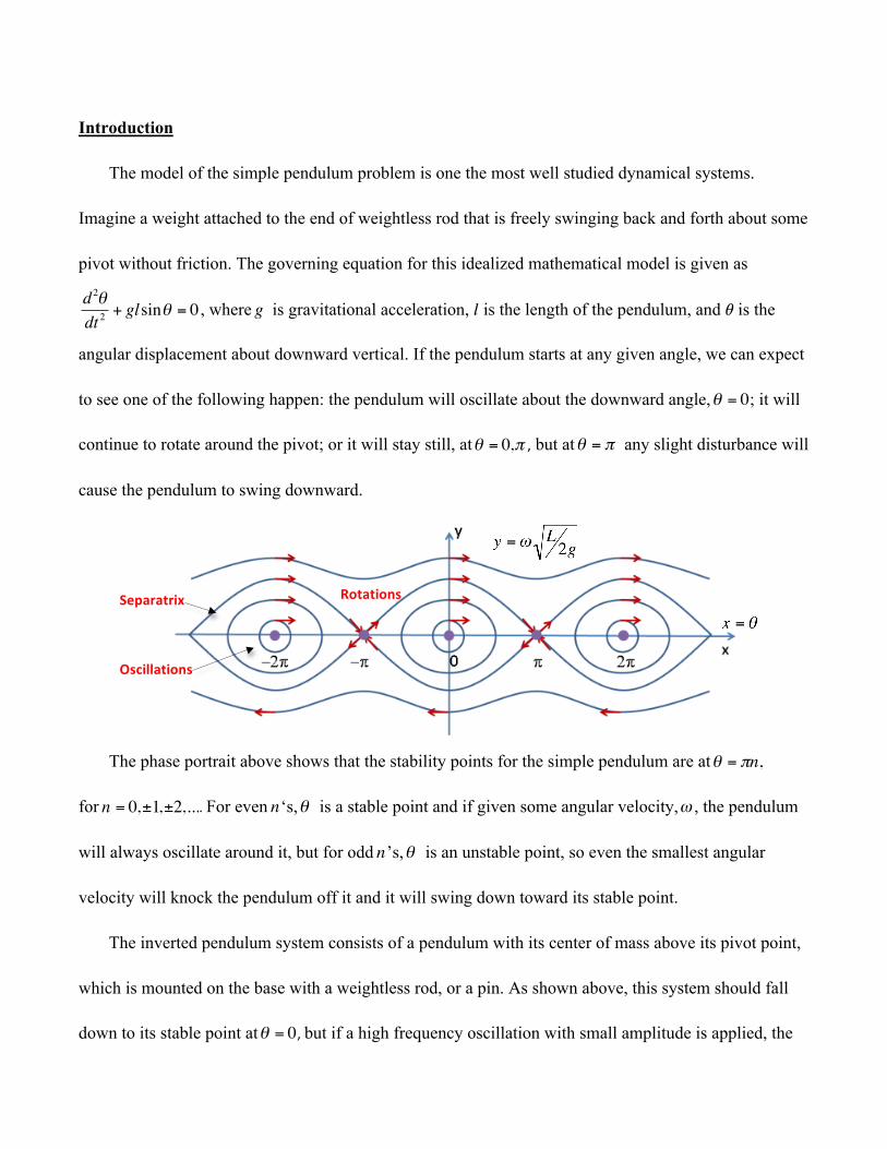
angular displacement about downward vertical. If the pendulum starts at any given angle, we can expect

to see one of the following happen: the pendulum will oscillate about the downward angle,

€

θ = 0; it will

continue to rotate around the pivot; or it will stay still, at

€

θ = 0,π , but at

€

θ = π   any slight disturbance will

cause the pendulum to swing downward.

The phase portrait above shows that the stability points for the simple pendulum are at

€

θ = πn,

for

€

n = 0,±1,±2,....  For even

€

n‘s,

€

θ is a stable point and if given some angular velocity,

€

ω , the pendulum

will always oscillate around it, but for odd

€

n’s,

€

θ is an unstable point, so even the smallest angular

velocity will knock the pendulum off it and it will swing down toward its stable point.

The inverted pendulum system consists of a pendulum with its center of mass above its pivot point,

which is mounted on the base with a weightless rod, or a pin. As shown above, this system should fall

down to its stable point at

€

θ = 0,  but if a high frequency oscillation with small amplitude is applied, the

Separatrix  

Oscillations  

Rotations  

inverted pendulum will stabilize. If this high frequency

oscillation is driven at an angle, it will create another oscillation

about its new stable point,

€

θ = π . This other oscillation has large

amplitude but low frequency. The goal of our study is to analyze

and simulate the stabilization of the inverted pendulum.

The study of the inverted pendulum system is more than

getting a pendulum to stay up right, its using the idea of

combining two different oscillations, one with high frequency

and small amplitude and the other with low frequency and large

amplitude, to stabilize an unstable point. The most obvious

application of the inverted pendulum is the segway because it is self-balancing, two-wheeled vehicle.

Another application that isn’t as straight forward would be a magnetic levitron. Permant magnets have

continuously changing electromagnetic field for a small distance away from it. So as one magnet lays on

a flat surface and another is placed on top, it will be repelled by the electromagnetic field, but if the top

magnet is spinning, than it can stabalize its leviate position above the other magnet. This also works for

any object that can be magnetized.

In our study, we will use a couple different methods to explain and prove this stability phenomenon.

First, like the simple pendulum problem, we will formulate an idealized model equation that describes

the pendulum’s motion over time. Using the Euler- Lagrange equation to derive the idealized model

equation of motion in dimensionless form,

€

d2θdτ 2

+ γ sinθ +αD(θ,τ ) = 0 . Next we will study the effective

potential energy of the driven pendulum. By averaging the potential energy over a period of the driving

oscillation, we can derive effective potential equation. Now we can study the stability of the pendulum

for different angles by applying the derivative test to the effective potential and create bifurcation

diagram based on our analysis. Then, with numerical analysis, we can confirm the stable angle using

MATlab’s ODE 45 method. MATlab solves the derived governing equation with three driving angles of

the pendulum and plots the result in phase portrait. In the future, we will look into graphically modeling

the behavior of the driven pendulum with a dynamic manifold. And after studying the theoretical

inverted pendulum, we will observe a real driven pendulum and compare the our predictions to the

actual behavior of the pendulum.

Model Equations

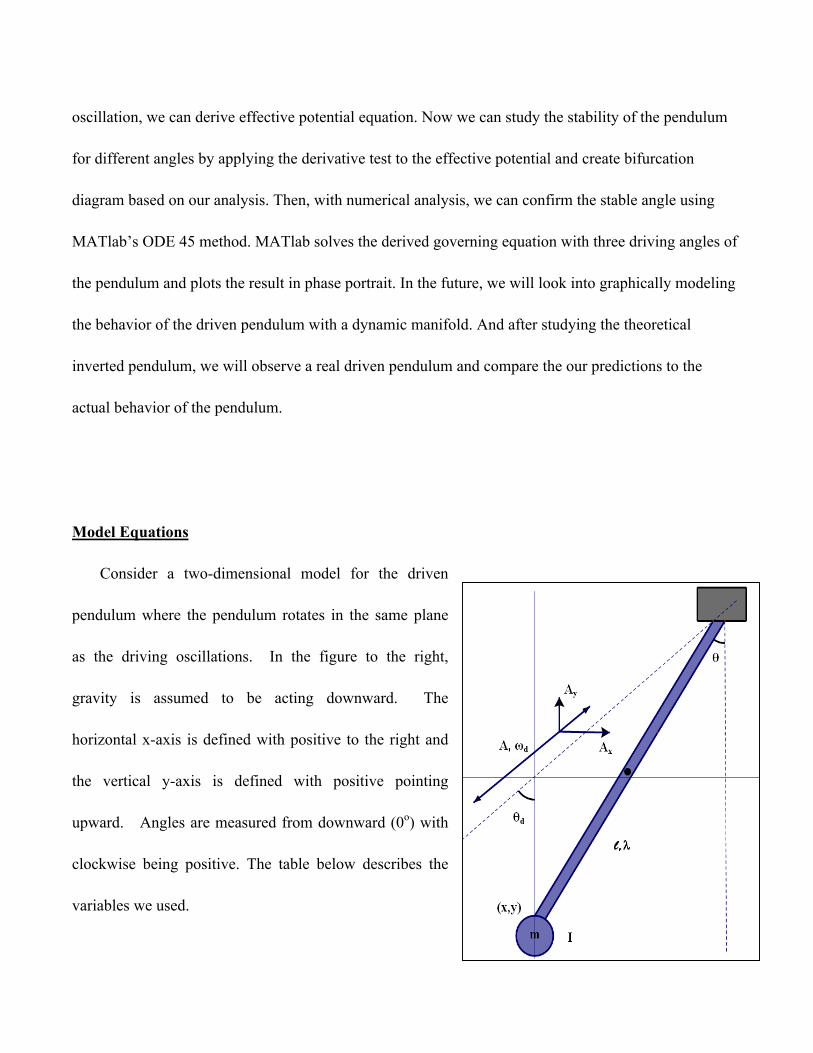
Consider a two-dimensional model for the driven

pendulum where the pendulum rotates in the same plane

as the driving oscillations. In the figure to the right,

gravity is assumed to be acting downward. The

horizontal x-axis is defined with positive to the right and

the vertical y-axis is defined with positive pointing

upward. Angles are measured from downward (0o) with

clockwise being positive. The table below describes the

variables we used.

Symbol Meaning

𝑡 Time

𝑥  ,  𝑦 Position of pendulum’s center of mass

𝑔 Acceleration due to gravity

𝜃 Angle of deviation of pendulum

𝑚 Mass of pendulum

𝑙 Distance from center of mass to base

𝐼𝑜 Rotational inertia about base

𝜆 Effective length of pendulum 𝐼𝑜𝑚𝑙2

𝜔𝑜 Natural frequency of pendulum 𝑔𝑙

𝜃𝑑 Drive angle of the base

𝜔𝑑 Drive frequency

𝐴𝑥  ,  𝐴𝑦 x- and y- amplitudes of the driving

We applied principles from Lagrangian mechanics and the Euler-Lagrange equation to the driven

pendulum in order to find the governing equation of motion. The Lagrangian for Newtonian

mechanics is the difference between the kinetic T and potential 𝑉 energies:

(1)

The equation of motion is derived from the Euler-Lagrange equation:

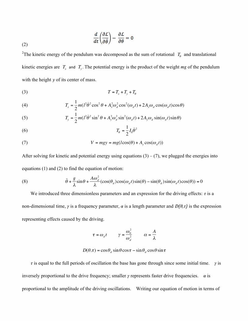
(2) 2The kinetic energy of the pendulum was decomposed as the sum of rotational

€

Tθ   and translational

kinetic energies are  

€

Tx   and  

€

Ty .  The potential energy is the product of the weight 𝑚𝑔 of the pendulum

with the height 𝑦 of its center of mass.

(3)

€

T = Tx +Ty +Tθ

(4)

€

Tx =12m(l2 ˙ θ 2 cos2θ + Ax

2ω d2 cos2(ω d t) + 2Axω d cos(ω d t)cosθ)

(5)

€

Ty =12m(l2 ˙ θ 2 sin2θ + Ay

2ω d2 sin2(ω d t) + 2Ayω d sin(ω d t)sinθ)

(6)

€

Tθ =12I0

˙ θ 2

(7)

€

V = mgy = mg(lcos(θ ) + Ay cos(ω d t))

After solving for kinetic and potential energy using equations (3) – (7), we plugged the energies into

equations (1) and (2) to find the equation of motion:

(8)

€

˙ ̇ θ +gλ

sinθ +Aω d

2

λ(cos(θd )cos(ω d t)sin(θ) − sin(θd )sin(ω d t)cos(θ)) = 0

We introduced three dimensionless parameters and an expression for the driving effects: 𝜏 is a

non-dimensional time, 𝛾 is a frequency parameter, 𝛼 is a length parameter and 𝐷(𝜃,𝜏) is the expression

representing effects caused by the driving.

€

τ =ω d t

€

γ =ω 02

ω d2    

€

α =Aλ

€

D(θ,τ ) = cosθd sinθ cosτ − sinθd cosθ sinτ

𝜏 is equal to the full periods of oscillation the base has gone through since some initial time. 𝛾 is

inversely proportional to the drive frequency; smaller 𝛾 represents faster drive frequencies. 𝛼 is

proportional to the amplitude of the driving oscillations. Writing our equation of motion in terms of

these dimensionless parameters gives us the non-dimensional form of the equation of motion:

(9)

€

d2θdτ 2

+ γ sinθ +αD(θ,τ ) = 0

Averaging Methods & Effective Potential

We applied averaging techniques and found the average or effective potential energy of the driven

pendulum. 1The effective potential 𝑈𝑒𝑓𝑓 will be a measure of the average potential energy the

pendulum has at certain pendulum angles of deviation 𝜃. We did this by averaging the potential energy

over a period of the driving oscillation. The first step is to separate the slow and fast components of

the pendulum. 𝜙 is the slower angle of the pendulum while 𝜉 is the rapid oscillations of the base. 𝐹(𝜃)

is the slower force of gravity while 𝑓(𝜃,𝜏) is the rapidly oscillating force from the driving.

(10)

€

I0˙ ̇ θ = I0( ˙ ̇ φ + ˙ ̇ ξ ) = (F(θ) + f (θ,t))

Considering 𝜉 as the difference between 𝜙 and 𝜃, we can do a first-order Taylor approximation to

(10). Making the assumption that 𝜉 is insignificantly small and 𝜔𝑑 is significantly large, we can ignore

negligible terms. After averaging the equation (10) over the period of oscillations of the base, we

derived equation (11).

(11)

€

I0˙ ̇ φ ≅ F(φ) +

ddθ

f (φ,t)ξ

Now, let’s define the 𝑈𝑒𝑓𝑓:

(12)

€

I0˙ ̇ φ = −

dUeff

dφ

Writing the forces using the terms from the equation of motion, we have:

€

F(θ) = −I0γ sinθ      

€

f (θ,t) = −I0αD(θ,t)

Using these expressions for force and plugging them into (11) and (12), we solved for 𝑈𝑒𝑓𝑓:

(13)

€

Ueff = I0 −γ cosθ +α 2

4(cos2θd sin

2θ + sin2θd cos2θ)

⎛

⎝ ⎜

⎞

⎠ ⎟

With 𝑈𝑒𝑓𝑓, we analyzed the stability of the pendulum for different 𝜃. Equilibrium angles 𝜃𝑒𝑞 are

predicted to occur where the derivative of (13) evaluates to zero:

(14)

€

dUeff

dθ= 0 = I0 sinθ

α 2

2(cos2θd cosθ eq ) + γ

⎛

⎝ ⎜

⎞

⎠ ⎟  

There are three different types of equilibrium angles: hanging down 𝜃𝑒𝑞=0, standing up 𝜃𝑒𝑞=𝜋, or

leaning to the side

€

θeq = ±arccos2(γα 2)cos2θd .  To  see  whether  these  equilibrium  angles  are  stable  

or  unstable,  we  looked  to  see  if  the  second  derivative  of  (13)  at  these  angles  is  positive  –  meaning  

stable  –  or  negative  –  meaning  unstable.  

(15)            

€

d2Ueff

dθ 2= I0

α 2

2(cos2θd cos

2θ eq ) + γ cosθ eq

⎛

⎝ ⎜

⎞

⎠ ⎟  

The conditions for stability are summarize in the table below for each equilibrium:

𝜽𝒆𝒒 Stable Unstable

0

€

γ >α 2

2cos2θd

€

γ < −α 2

2cos2θ

€

±arccos2(γα 2)cos2θd

€

4γ 2α 2 −α 2

2cos2θd > 0

€

4γ 2α 2 −α 2

2cos2θd < 0

𝜋

€

γ <α 2

2cos2θd

€

γ >α 2

2cos2θd

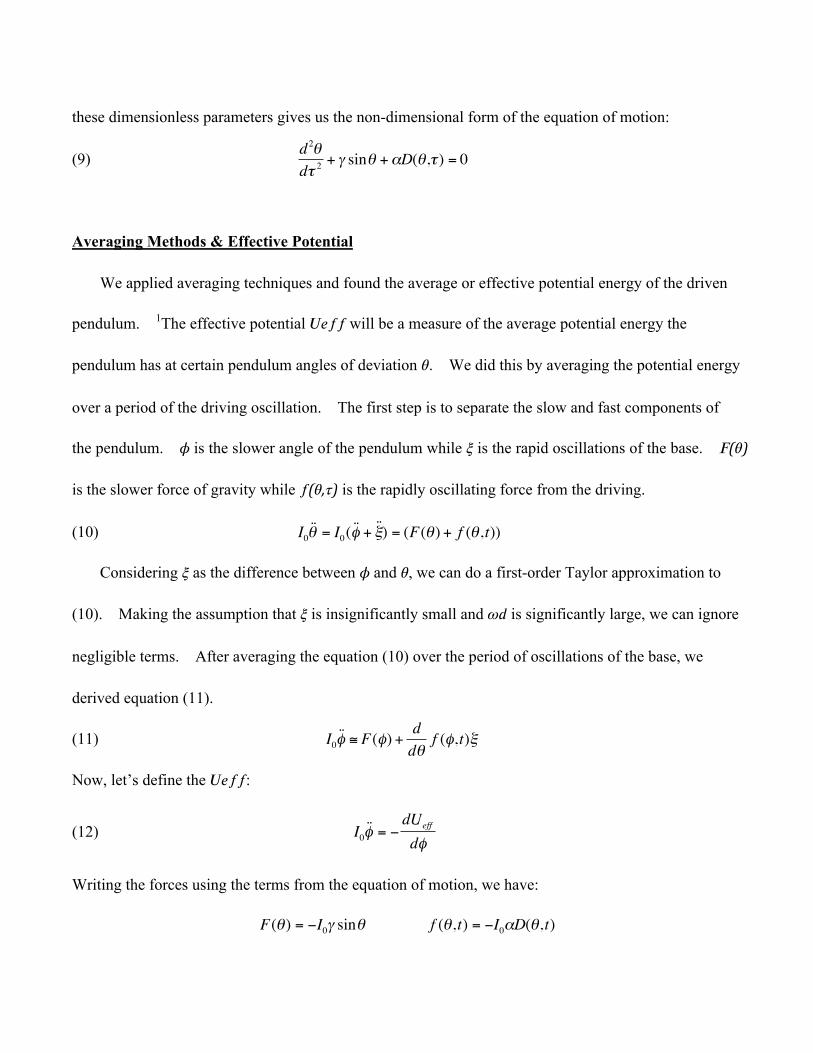
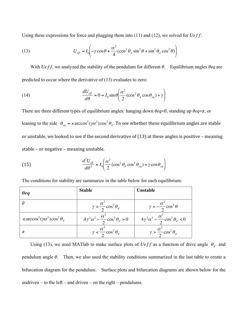
Using (13), we used MATlab to make surface plots of 𝑈𝑒𝑓𝑓 as a function of drive angle

€

θd and

pendulum angle 𝜃. Then, we also used the stability conditions summarized in the last table to create a

bifurcation diagram for the pendulum. Surface plots and bifurcation diagrams are shown below for the

undriven – to the left – and driven – on the right – pendulums.

Numerical Study

Using the derived governing equation of motion (9) from the Lagrangian analysis, we can take a

numerical look at how any particular pendulum will behave when driven at any particular angle. For the

purposes of our analysis, we are using the parameters associated with our Black and Decker jigsaw,

including its effective length, driving frequency, and driving amplitude, and will change our angular

displacement to be about the upward vertical. By implementing MATlab’s ODE45 method, we can set

the initial angle and initial velocity for the pendulum and plot the solution for the pendulum’s angle vs.

the time passed since the pendulum’s release. ODE45 uses a Runge-Kutta variable step method to solve

our differential equation, which MATlab then plots. First we plot the non-driven pendulum so that we

can compare the graphs of a pendulum driven at high and low frequencies with a simple case.

• stable  • unstable  

Still using this method, we will compare the behavior of a driven pendulum at three different driving

angles: 𝜃=0,  drives  about  the  vertical; 𝜃=𝜋/4, drives about the diagonal; and 𝜃=𝜋/2,  drives about the

horizontal.

For the sake of avoiding redundancy, symmetrical angles have been disregarded. By setting

appropriate initial conditions, we have observed oscillatory behavior for each driving angle, indicating

the stability points therein. As expected, the stability point for the horizontal driving angle is located

below the horizontal, due to gravity. Notably, the diagonal driving angle has produced differing results

from the other two driving angles. It oscillates about 𝜃=0, as expected, but with lengthy and wide

oscillations. This is most likely due to the volatility of the equilibrium angle as the angle slightly

increases from 𝜃=𝜋/4. Further analysis and experimentation will test the accuracy of this model with the

actual behavior of the jigsaw.

Work Cited

1Shew,  Woody.   “Inverted   Equilibrium   of   a   Vertically   Driven   Pendulum”.  wooster.edu.   College   of  

Wooster.  24  Apr,  1997.  Web.  23  Mar,  2013.  

2VanDalen  J.,  Gordon.  “The  driven  pendulum  at  arbitrary  drive  angles”.  arvix.org.  Department  of  

Physics  at  University  of  California  and  Embry-­‐Riddle  Aeronautical  University.  2  Feb,  2008.  

Web.  24  Mar,  2013.