THE INVERTED PENDULUM

A Design Project Report

Presented to the Engineering Division of the Graduate School

of Cornell University

in Partial Fulfillment of the Requirements for the Degree of

Master of Engineering (Electrical)

By

John Stang

Project Advisor: Dr. Bruce Land

Degree Date: May, 2005

II

Abstract

Master of Electrical Engineering Program

Cornell University

Design Project Report

Project Title: The Inverted Pendulum

Author: John Stang

Abstract: The inverted pendulum is a classical control problem, which involves developing a

system to balance a pendulum. For visualization purposes, this is similar to trying to balance a

broomstick on a finger. To study this problem, this project incorporated a full system design

including all of the mechanical, hardware, and software design at minimal cost. There are three

main subsystems that compose this design: (1) the mechanical system, (2) the feedback network

which includes sensors and a method to read them, and (3) a controller and its interface to the

mechanical system. After determining sets of requirements between the subsystems, each one

can be designed independent of the other two, simplifying the design process. The mechanical

design involved building a track, cart, pendulum, and drive mechanism. The track, cart, and

pendulum were developed out of primarily aluminum and wood. The drive mechanism is a DC

motor with a sprocket mounted onto its shaft to pull a chain, which the cart connects to. The

feedback network consisted of rotational potentiometers, which were sampled by an analog-to-

digital converter, to measure the angle of the pendulum and the displacement of the cart. The

controller was implemented by an Atmel Mega32 which varies the speed of motor by using pulse

width modulation. The final system results in a cart that could balance a pendulum for a limited

amount of time. This was due to many imperfections in the mechanical system and the inability

to model the dynamics of these imperfections along with the calculation limitations of the Atmel

Meg32.

Report Approved by

Project Advisor: _______________________________________________Date:_____________

III

Executive Summary

The classic control problem of the inverted pendulum is interesting in that it can be solved using

a wide variety of systems and solutions. This problem is similar to trying to balance a

broomstick on a finger. The flexibility of this problem invites those interested in system design,

control theory, and just plain problem solving to try and develop a working system. For this

project, the motivation was to translate the mathematical models developed in control theory

classes into a real-time system. This design is a full system design including all of the

mechanical, hardware, and software aspects at minimal cost.

The design process for this project required a great deal of planning and testing before deciding

on a final design since there were so many alternatives to choose from. The design problem can

be broken down into subsystems which are extremely dependent on each other. The actual

design of each subsystem was an iterative process of testing components and implementing

simple solutions until the “optimal” solution could be found. The “optimal” solution can be

defined as the solution that can be developed at minimal cost (meeting budget constraints) which

balances the pendulum the best.

During the design process, many setbacks were encountered. The most important and time

consuming setbacks all related to broken motors. When the first motor broke, a faster and higher

torque motor was obtained because the original one was not able to react fast enough in order to

balance the pendulum. Since the new motor had different dimensions than the first, the whole

mechanical system needed to be redesigned. The next two motors broke when the control effort

was too high and changing direction rapidly, putting too much stress on the internal gears. To

fix this, the controller was redesigned with a tighter constraint on the control effort.

In the end, a system and controller were designed to balance the pendulum for about 3-5 seconds

before reaching the edge of the track. Applying small “taps” to the pendulum in the opposite

direction would allow for much longer control. The final result of this design process can be

deemed a success since a working mechanical system was developed with an optimal controller

designed by minimizing the Linear Quadratic Regulator cost equation, given the maximum

desired angle, displacement, and control effort.

IV

Table of Contents

INVERTED PENDULUM IABSTRACT IIEXECUTIVE SUMMARY III1. INTRODUCTION 1 1.1 MOTIVATION 1 1.2 BACKGROUND 12. DESIGN PROBLEM AND REQUIREMENTS 3 2.1 THE PROBLEM 3 2.2 THE CONSTRAINTS 3 2.3 THE REQUIREMENTS 33. THE RANGE OF POSSIBLE SOLUTIONS 5 3.1 MECHANICAL SYSTEM 5 3.1.1 TRACK, CART, AND PENDULUM 6 3.1.2 THE MOTOR AND THE CONTROL CIRCUIT 8 3.2 FEEDBACK NETWORK 9 3.2.1 DISPLACEMENT SENSORS 10 3.2.2 ANGLE SENSORS 12 3.3 CONTROLLER SOLUTIONS 12 3.3.1 MODELING THE SYSTEM DYNAMICS 13 3.3.1.1 MODELING ASSUMPTIONS 13 3.3.1.2 LINEARITY 13 3.3.1.3 COMPLEXITY 13 3.3.2 CONTROLLER DESIGN 14 3.3.2.1 CLASSICAL CONTROL 14 3.3.2.2 MODERN CONTROL 14 3.3.2.3 ROBUST CONTROL 16 3.3.2.4 MODEL PREDICTIVE CONTROL 17 3.3.3 CONTROLLER IMPLEMENTATION 18 3.3.4 THE FINAL DESIGN CHOICES AND REASONING 19 3.3.4.1 THE FINAL DESIGN CHOICES 19 3.3.4.2 THE REASONING BEHIND THE CHOICES 194. DESIGN PROCESS AND IT’S IMPLEMENTATION 21 4.1 MECHANICAL SYSTEM 21 4.2 FEEDBACK NETWORK 26 4.3 CONTROL CIRCUIT 27 4.4 SYSTEM MODEL AND CONTROLLER IMPLEMENTATION 27 4.4.1 THE SYSTEM DYNAMICS 28 4.4.2 THE STATE SPACE MODEL 32 4.4.3 LQR CONTROLLER DESIGN 35 4.4.4 USING THE MEGA32 TO APPLY THE CONTROL LAW 39 4.4.4.1 PARAMETERIZING THE MOTOR 39 4.4.4.2 IMPLEMENTING THE CONTROL LAW 41 4.5 EVOLUTION OF THE REQUIREMENTS 425. RESULTS COMPARED TO EXPECTATIONS 43

V

6.CONCLUSION 467. REFERENCES 478. ACKNOWLEDGEMENTS 48APPENDIX A: SCHEMATICS 49APPENDIX B: INSTRUCTION MANUALS 50 B.1. HOW TO PARAMETERIZE THE MOTOR 50 B.2. HOW TO OPERATE THE CONTROLLER 50APPENDIX C: C SOURCE FILES AND MATLAB M-FILES FOR PARAMETERIZING THE MOTOR

51

C.1. C SOURCE FILE 51 C.2. MATLAB DATA ACQUISITION PROGRAM 58 C.3. MATLAB PARAMETER CALCULATIONS 60APPENDIX D: MATLAB FILE FOR DESIGNING A CONTROLLER 65APPENDIX E: C SOURCE FILE FOR THE CONTROLLER 68APPENDIX F: PARTS LIST AND COST 73APPENDIX G: PICTURES OF THE OVERALL DESIGN 74

1

1. Introduction

1.1 Motivation

My educational experience at Cornell University has given me a broad background in many of

the fields in Electrical and Computer Engineering such as microcontroller design, digital signal

processing (DSP), control theory, etc. For a Master’s of Engineering project, I hoped to integrate

design techniques from multiple fields in creating a system. Since my current interests lie within

microcontroller design, control theory, and DSP, I decided to design and build an unstable

system and then a controller that would stabilize it using feedback control techniques. Most of

my control experience had been simulating mathematical models using Matlab. My hopes were

to design a controller that would work in theory and then figure out how to translate a

mathematical representation of that controller into a working model. After much thought, I

decided the classic control problem of the inverted pendulum was the perfect problem to do this

with. I had dealt with this problem in ECE 472, Feedback Control Systems, in two of the

laboratory experiments, but the extent of the design was to come up with a mathematical model

of a controller and then upload it into an existing system to test the controller. On the other

hand, this project will be the complete system design including all of the mechanical, hardware,

and software design that can be done at minimal cost.

1.2 Background

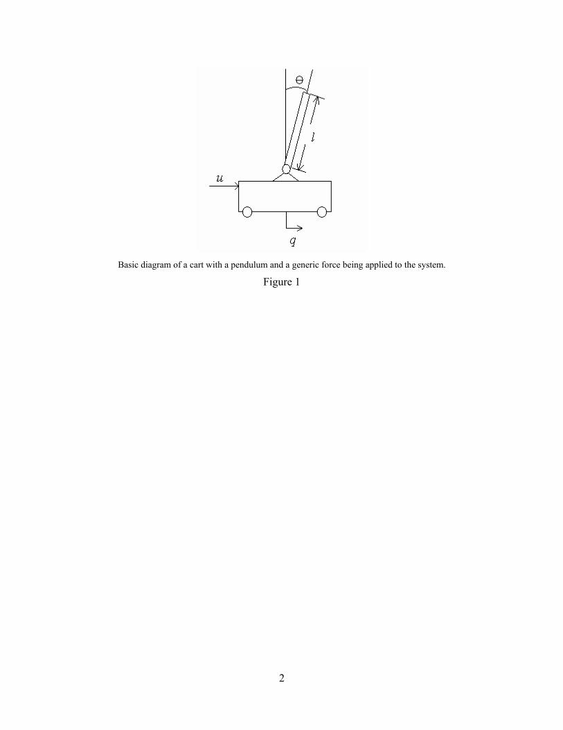
The inverted pendulum is a system that has a cart which is programmed to balance a pendulum

as shown by a basic block diagram in Figure 1. This system is adherently instable since even the

slightest disturbance would cause the pendulum to start falling. Thus some sort of control is

necessary to maintain a balanced pendulum. An ideal controller would keep the pendulum

balanced with very little change in the angle, θ, or cart displacement, q. Obviously limitations

would be imposed based on the actual parameters of the system as well as the method for

implementing a controller. Thus designing a controller that is close to ideal is a challenging

design problem.

2

Basic diagram of a cart with a pendulum and a generic force being applied to the system.

Figure 1

3

2. Design Problem and Requirements

2.1. The Problem

The goal of this project is to design a mechanical system for the inverted pendulum problem and

then implement a feasible controller using the Atmel Mega32 as the main processing unit. The

controller should minimize both the displacement of the cart and the angle of the pendulum. The

system should be standalone and easy to use such that other controllers can be implemented as

desired.

2.2. The Constraints

The assembly of the mechanical system, requires access to a variety of tools and the assistance of

certified users of various machine shops. Since assistance is required, the ability to machine

parts is limited, and thus the design has to be relatively simple such that the number of iterations

of building and testing the system are relatively few.

Another limiting factor in this design is the budget. Since this project does not support any

research at Cornell University, it is not funded by the university. Thus the project needs to be

low cost. To minimize cost, some parts were sampled and others were chosen not because they

were the best choice, but the best choice that was affordable. Components such as the motor

suffer because of this constraint.

2.3. The Requirements

To design any system, a set of requirements is necessary to have guidelines when making

decisions about implementation. This project is no different. Taking the constraints into

consideration, a set of requirements and goals was established for this project as follows:

• Working mechanical system.

• Good Interface between the Atmel Mega32 and the mechanical system.

• Well designed accurate sensors.

• Matlab interface (Visual and data extraction).

• Easily programmable through user interface to allow other solutions.

• Main solution should balance for an extended period of time (at least 10 seconds).

4

• System is self-contained except for programming purposes and data extraction.

• Nonlinear Control (if time permits).

• Double inverted pendulum (if time permits).

• Wireless Sensors (if time permits).

As the project progresses it is expected that some of these requirements will change as necessary.

A modified list of requirements will be included at the end of the design section outlining what

was actually feasible.

5

3. The Range of Possible Solutions

Due to the modularity of this project, the system can be broken up into many subsystems, as

shown in Figure 2, that can each be solved in a variety of ways.

Block Diagram of the Overall System.

Figure 2

It is necessary to realize that each module can be solved in its own way, but to design a solution

for a specific module, it is imperative to have some knowledge of the other modules. Thus this

design process must take a gray box approach. For this discussion, each module will be

discussed with a variety of solutions presented. The final design choices will be outlined at the

end of this section explaining the reasoning for the choice and demonstrating how the

dependence between subsystems had an affect on these decisions. Note that the solutions given

in this section are not inclusive. One could easily imagine many other solutions to this problem.

3.1. Mechanical System

The design of a mechanical system for this project involves integrating four main components:

(1) the cart, (2) the pendulum, (3) the track, and (4) the mechanism used to move the cart. There

are many ways to implement these, though each component is quite dependent on the other three.

These components also have to meet some basic requirements such that it is possible to design a

controller to balance the pendulum. These requirements are as follows,

• The cart motion needs to be limited to one degree of freedom which is in the horizontal

plane.

• The pendulum motion needs to be limited to two degrees of freedom, one of which is the

same as the cart’s degree of freedom.

6

• The friction that impedes the cart and pendulum motion must be reduced as much as

possible.

3.1.1. Track, Cart, and Pendulum Solutions

One solution would be to have a U-channel track within which the cart would move. Ideally, the

cart would fit well in the track and slide smoothly with little friction. Also needed in this design

is a mechanism to apply force on the cart in either direction. This could be done in one of two

ways. The first way would be to mount a motor at the end of the track with a drive

wheel/sprocket attached to the shaft and another wheel/sprocket free-spinning at the opposite end

of the track. Around the two wheels would be a pulley or chain with which the cart can be fixed

to. The second way would be to have a motor directly drive wheels on the bottom of the cart.

This solution will not be considered since the design of adding a motor to the cart for a

reasonable size U-channel (2 inch width) would be too complex and intricate. Below is a simple

rating of this solution based primarily on the basic requirements outlined at the beginning of this

section.

• Pros

o 2 degrees of freedom for the pendulum.

o 1 degree of freedom for the cart.

o Simple cart design.

• Cons

o Friction could be a problem.

o Drive Mechanism could be complicated.

o More room for error with the integration of multiple systems (drive mechanism

can be considered its own system).

A second option for the mechanical design could have the motor as the main component of the

cart. In this design, depending on the size of the motor, the cart can be built around the motor.

The motor would have a teethed drive wheel mounted on its shaft which would fit into a teethed

track that is flat on the surface. In order to guarantee that the drive wheel does not come off the

track, a guide will need to implemented such that it is parallel to the track that the cart would be

7

attached too. One possible guide could be a long steel rod with which the cart could have an arm

to wrap around.

• Pros

o Overall System is compact.

o Could be self contained if controller is mounted on the cart as well.

o Reduced Friction.

o Good ability to change direction quickly.

• Cons

o Cart design may be complex.

o Guide may be hard to integrate.

o Possible slip condition with drive wheel and track.

A variation of the second option would be to not have a track- just have a cart with the pendulum

still mounted on top. This cart would be self contained with the whole system integrated in the

cart itself. The motor would control a set of wheels that would move to keep the pendulum

balanced. This design would not need a guide since the center of mass of this design would be

low to the ground. A gear assembly may be necessary to drive to wheels simultaneously. It

could be possible to have one wheel centered on one side with free spinning wheels on the other

that could work satisfactory without any gear assembly.

• Pros

o Overall System is compact.

o Self Contained.

• Cons

o Reaction time is dependent on motor torque and the strength of the friction

between the wheels and ground surface.

o Cart may have more than 1 degree of freedom.

o Pendulum may have more than 2 degrees of freedom.

o Displacement may be hard to measure since there is no reference point to measure

against.

8

One other intriguing solution would be to have the motor with a rod mounted on the shaft such

that when the motor turns, the rod is parallel to the ground. Attached to the end of this shaft

would be the pendulum. Thus this system would have a circular motion instead of the linear

displacement previously discussed.

• Pros

o Cart is simply the rod.

• Cons

o Strong motor needed.

o System must be well built such that the rod is strongly attached to the motor shaft.

o Nonlinearities of the motion of the cart will be difficult to model.

Other variations of the mechanical system include using any of the suggested solutions with

pendulums of different shapes, lengths, mass distributions, etc. The ideal case for the inverted

pendulum problem, which is the easiest to model is the pendulum with all the mass located at the

tip. This allows for the approximation of the moment of inertia of the pendulum to be zero.

3.1.2. The Motor And The Control Circuit

There are three main choices to use for motors for this project: (1) a DC motor, (2) a stepper

motor, and (3) a servo motor. The two main considerations in choosing a motor are the needs for

high torque and high speed. The torque is necessary for the cart to change direction quickly in

order to keep the pendulum balanced. High speed is needed such that the cart can move faster

than the pendulum can fall.

The DC motor could have high torque and high speed, but it comes at a cost. First of all, when

the torque and speed of a DC motor increase, it requires more power to run the motor. This will

be limited by the circuitry used to control the motor. The control circuitry for a DC motor is

typically an H-bridge which controls the direction of current across the motor based on the

directional signal. Another input to the H-bridge controls the speed of the motor. The second

cost of having a good DC motor is that they can be quite expensive.

9

The stepper motor could provide high torque, but it would lack sufficient speed. A bi-polar

stepper would be necessary to ensure that the motor turns both directions. For this motor, there

are four inputs lines that need to be toggled in the correct order to have the motor turn in a

certain direction and in the opposite order for the motor to move in the reverse direction. This

control can be done externally through the use of digital logic components that would require

just a directional signal and a speed control, but this would make the design more complex.

Instead a simpler solution would have four control lines come directly out of the MCU. Stepper

motors are also costly and consume a great deal of power.

The servo motor could supply high speed, but would suffer with the torque. It would also be

harder to incorporate into this design. First off, servo motors typically have the ability to turn

only 360°. In order to have such a motor, the drive wheel attached to the motor shaft would have

sized such that one rotation could cause the cart to travel the length of the track. This would

require a large wheel would decrease the amount of torque provided by the motor and could

possible damage the motor. Also note that controlling a servo motor could be quite difficult in

this application since the voltage level applied to the motor tells the motor which angle to be at.

There is less intuition in designing controller that operates in this way.

Regardless of which motor is chosen, a separate power supply will be necessary just for the

motor. The large power consumption by the motors and the inductive spikes created each time

the motor changes direction could be harmful to any other circuit hooked up to the same power

supply. The only way to control the motor would be through opto-islolation which completely

separates circuits with different power supplies.

3.2. Feedback Network

Designing an accurate feedback network is essential to stabilizing the system. Thus the sensors

need to relatively noiseless and have a fast response such that the information retrieved from the

sensors accurately reflects the state of the system. Determining the variables of the system to

measure can be difficult. In this case there are four parameters that govern the inverted

pendulum system (which will be derived in a later section). They are (1) the angle, (2) the

angle’s velocity, (3) the displacement of the cart, and (4) the velocity of the cart. Thus there are

10

four measurable parameters that could be used for feedback, which would determine the control

necessary to stabilize the system. Most conventional approaches to this problem only measure

the angle and displacement and derive the other two parameters from these. This project follows

in suit since those two parameters are the easiest to measure and give the most information about

the system.

When gathering information from the sensors it will be necessary to have sensors that produce a

variable voltage output that can be sampled by the Mega32. The Mega32 will be programmed to

use its internal Analog-to-Digital Converter (ADC) to convert the voltage outputs of the sensors

into a binary representation which then can be converted into a usable measurement. The

internal ADC runs as fast as 15kHz, but can only perform one conversion at a time so the

Mega32 will alternate between the two sensors. It may be possible to incorporate faster and

more accurate external ADCs, but it will require a larger I/O interface and accurate timing to

guarantee good readings.

3.2.1. Displacement Sensors

One way to measure displacement would be to attach a potentiometer to either the drive sprocket

or the free-spinning one. The voltage on the wiper of the potentiometer would then be converted

to a digital signal by an ADC. It is then possible to determine the displacement of the cart by

using the diameter of the sprocket, the measured voltage, and the number of turns the

potentiometer is capable of.

• Pros

o Easy Implementation.

• Cons

o Potentiometer output voltage may be nonlinear.

o Sampling frequency may be limited by ADC conversion time thus reaction time

by the controller is limited.

o Accuracy is limited by two factors.

Potentiometer is accurate to within a tolerance.

ADC is accurate to within a tolerance

11

Another option could be a linear potentiometer. This could be mounted to the track with the

slider attached to the cart. Similar sampling methods would then be implemented using an ADC.

• Pros

o Easy Implementation.

• Cons

o Expensive since most linear potentiometers are only tens of centimeters long and

this project may have tracks approximately 1.5 meters long.

o Sampling frequency may be limited by ADC conversion time thus reaction time

by the controller is limited.

o Accuracy is limited by two factors.

Potentiometer is accurate to within a tolerance.

ADC is accurate to within a tolerance.

Another possibility could be to have light sensors spaced parallel to the track with a receiver on

the other side of the track. These would work by signaling when the cart has passed between an

emitter and receiver breaking the signal.

• Pros

o Simple Concept.

• Cons

o Accuracy is limited to the spacing of the sensors.

o Many sensors necessary for an accurate reading.

Radar and sonar sensors are also possible. These would emit a light or sound, respectively, and

wait for the reflection. The time it takes for a reflection would be used to then calculate the

distance. Unfortunately these sensors are more expensive and could take up a great deal of

processing time which would slow down the reaction of the system. Thus they will not be

considered for this project.

12

3.2.2. Angle Sensor

One of the easiest solutions would be to mount the pendulum on a circular potentiometer.

Ideally, the potentiometer would have little friction. Though practical potentiometers will have

some friction, which could influence the dynamics of the pendulum falling. More friction would

slow down the reaction of the pendulum to any of the forces exerted on it, making it easier to

balance.

• Pros

o Easy Implementation.

• Cons

o Potentiometer output voltage may be nonlinear.

o Friction of potentiometer may influence the dynamics of the pendulum falling.

o Sampling frequency may be limited by ADC conversion time thus reaction time

by the controller is limited.

o Accuracy is limited by two factors.

Potentiometer is accurate to within a tolerance.

ADC is accurate to within a tolerance

A hub encoder could be another practical solution. This sensor reads the angle and then returns

the digital representation to the Mega32. Unfortunately this sensor is expensive and will not be

considered.

3.3. Controller Solutions

Once a mechanical system is developed with an accurate feedback network and an easy interface

for controlling the cart, a controller can be designed. As this section will show, there are many

ways to implement a working controller. The largest constraint of designing a working

controller, is how well the system is modeled. If the system has mismodeled or unmodeled

dynamics, it is quite likely the controller designed from this model will not work. This section

will discuss the modeling of the system and the necessary assumptions that required to design

and implement a working controller. Once the modeling techniques have been discussed,

possible controller design approaches will be presented.

13

3.3.1 Modeling the System Dynamics

In general, an accurate model of the system is desired. Unfortunately, modeling a system

accurately may make it very difficult to design a controller. Most control techniques hinge on

the assumption that the system is linear. Thus simplifications will need to be made in hopes that

the resulting model is still a relatively accurate model of real system.

3.3.1.1. Modeling Assumptions

A first approach to modeling would be to assume a frictionless system with all motion limited to

the desired degrees of freedom. This may not seem like a fair approach since the system indeed

has friction.. If friction was included in the model, the system may become very complex, thus

making it difficult to design for. It is also quite possible to mismodel the friction given a

mechnical system that is relatively complex. One way to compensate for not modeling the

friction is account for it while measuring certain parameters of the system. This will be

discussed in Section 4.4.4.

3.3.1.2. Linearity

The inverted pendulum is adherently a nonlinear system due to the cosine and sine terms

generated while modeling the pendulum. Assuming that the pendulum’s angle will remain

small, since there should be ample control to keep it balanced, it may be possible to approximate

sin θ = θ and cos θ = 1. Thus this will linearize the system, which will allow for controller

design methods to use linear system techniques.

Designing for a non-linear system may be quite difficult and will not be addressed in this project.

3.3.1.3. Complexity

Another assumption that may be made which will greatly reduce the complexity of the system is

that all of the mass of the pendulum is located at the tip. This will allow for the moment of

inertia of the pendulum to be zero, which simplifies the system dynamics.

14

3.3.2. Controller Design

Control Theory has evolved over the past 75 years. There has been the classic control era,

modern control era, robust control era, and now the model predictive era. Thus there are many

viable solutions for designing a controller specific to this system. Though when implementing

these solutions, the Mega32 may impose constraints in timing and calculation ability which need

to be considered.

3.3.2.1. Classical Control

One possible way to design a controller for this problem would be to use classical control

techniques. In general classical control is used on Single Input Single Output (SISO) systems,

but can be applied to Multiple Input Multiple Out (MIMO) systems using clever manipulations

of the dynamics. One possible manipulation to change a MIMO system into a SISO system

would be to combine the measurements into a “virtual” measurement. This would only work in

certain situations where the measurements can be correlated. In this case, the displacement can

be related to the angle.

• Pros

o Many design tools.

Bode Plots.

Root Locus.

Nichols/Nyquist Plots.

o Simple Implementation.

• Cons

o Better suited for SISO systems and the “virtual” measurement may be inaccurate.

o Many design variables could make for a long iterative process.

3.3.2.2. Modern Control

Modern Control may seem like the most logical choice for this design since this technique is

focuses primarily on Multiple Input Multiple Output (MIMO) systems. The main design

objective is to minimize the cost equation which is an integral over time of the weighted inputs

and outputs. There are two cost equations that are typically used for this design technique. There

15

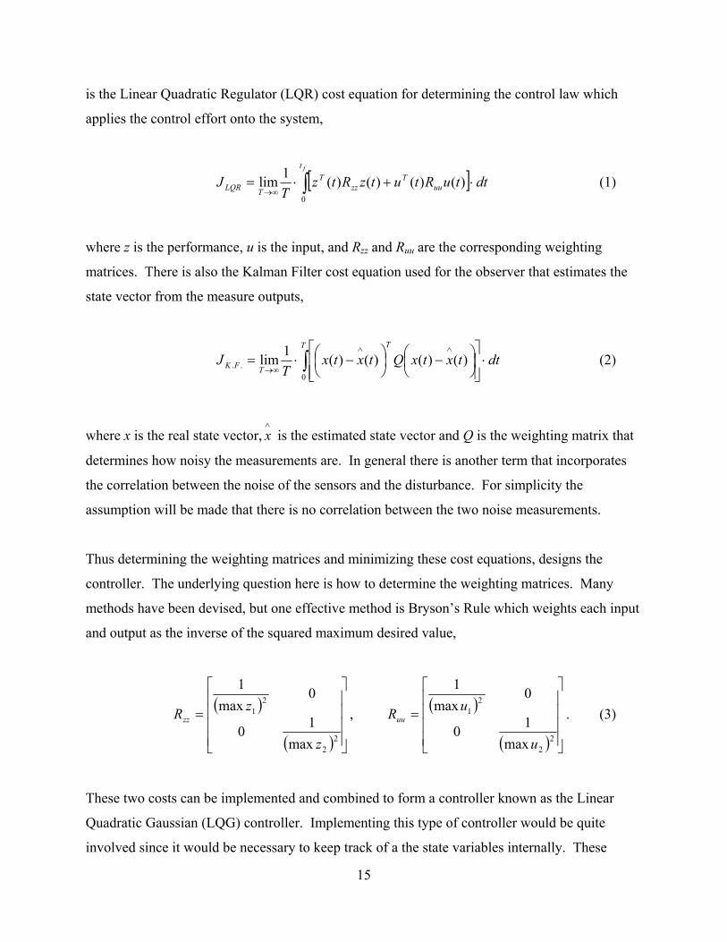
is the Linear Quadratic Regulator (LQR) cost equation for determining the control law which

applies the control effort onto the system,

[ ]∫ ⋅+⋅=∞→

ft

uuT

zzT

TLQR dttuRtutzRtzT

J0

)()()()(1lim (1)

where z is the performance, u is the input, and Rzz and Ruu are the corresponding weighting

matrices. There is also the Kalman Filter cost equation used for the observer that estimates the

state vector from the measure outputs,

∫ ⋅⎥⎥⎦

⎤

⎢⎢⎣

⎡⎟⎠⎞

⎜⎝⎛ −⎟

⎠⎞

⎜⎝⎛ −⋅=

∧∧

∞→

T T

TFK dttxtxQtxtxT

J0

.. )()()()(1lim (2)

where x is the real state vector,∧

x is the estimated state vector and Q is the weighting matrix that

determines how noisy the measurements are. In general there is another term that incorporates

the correlation between the noise of the sensors and the disturbance. For simplicity the

assumption will be made that there is no correlation between the two noise measurements.

Thus determining the weighting matrices and minimizing these cost equations, designs the

controller. The underlying question here is how to determine the weighting matrices. Many

methods have been devised, but one effective method is Bryson’s Rule which weights each input

and output as the inverse of the squared maximum desired value,

( )

( ) ⎥⎥⎥⎥

⎦

⎤

⎢⎢⎢⎢

⎣

⎡

=

22

21

max10

0max

1

z

zRzz , ( )

( ) ⎥⎥⎥⎥

⎦

⎤

⎢⎢⎢⎢

⎣

⎡

=

22

21

max10

0max

1

u

uRuu . (3)

These two costs can be implemented and combined to form a controller known as the Linear

Quadratic Gaussian (LQG) controller. Implementing this type of controller would be quite

involved since it would be necessary to keep track of a the state variables internally. These

16

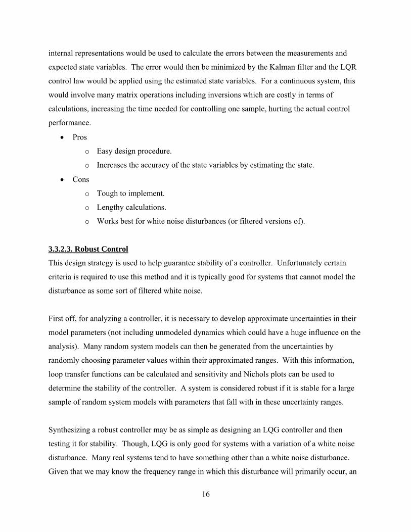
internal representations would be used to calculate the errors between the measurements and

expected state variables. The error would then be minimized by the Kalman filter and the LQR

control law would be applied using the estimated state variables. For a continuous system, this

would involve many matrix operations including inversions which are costly in terms of

calculations, increasing the time needed for controlling one sample, hurting the actual control

performance.

• Pros

o Easy design procedure.

o Increases the accuracy of the state variables by estimating the state.

• Cons

o Tough to implement.

o Lengthy calculations.

o Works best for white noise disturbances (or filtered versions of).

3.3.2.3. Robust Control

This design strategy is used to help guarantee stability of a controller. Unfortunately certain

criteria is required to use this method and it is typically good for systems that cannot model the

disturbance as some sort of filtered white noise.

First off, for analyzing a controller, it is necessary to develop approximate uncertainties in their

model parameters (not including unmodeled dynamics which could have a huge influence on the

analysis). Many random system models can then be generated from the uncertainties by

randomly choosing parameter values within their approximated ranges. With this information,

loop transfer functions can be calculated and sensitivity and Nichols plots can be used to

determine the stability of the controller. A system is considered robust if it is stable for a large

sample of random system models with parameters that fall with in these uncertainty ranges.

Synthesizing a robust controller may be as simple as designing an LQG controller and then

testing it for stability. Though, LQG is only good for systems with a variation of a white noise

disturbance. Many real systems tend to have something other than a white noise disturbance.

Given that we may know the frequency range in which this disturbance will primarily occur, an

17

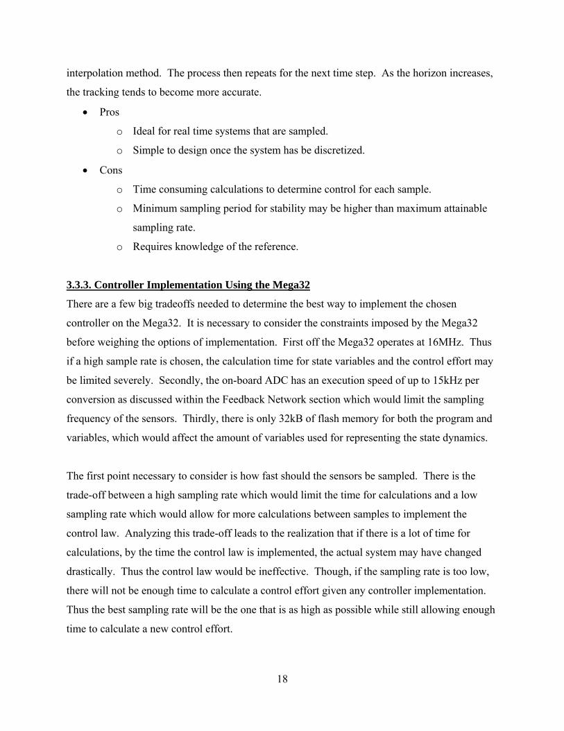
extra term with parameter γ can be added into the cost equation as shown in Eq. (4) to

incorporate the distanbance, d, when determining the controller.

[ ]∫ ⋅++⋅=∞→

ftT

uuT

zzT

TLQG dtddtuRtutzRtzT

J0

2)()()()(1lim γ (4)

Minimizing γ until the system is close to instability gives the H∞ control law. As γ approaches

infinity we get the LQG controller and anywhere in between is considered H2 control.

• Pros

o Handles non-white noise disturbances

o Better chance for stability assuming the system is not mismodeled.

• Cons

o Tough to implement

o Lengthy calculations

o Set up for analysis requires some educated guesses about the system

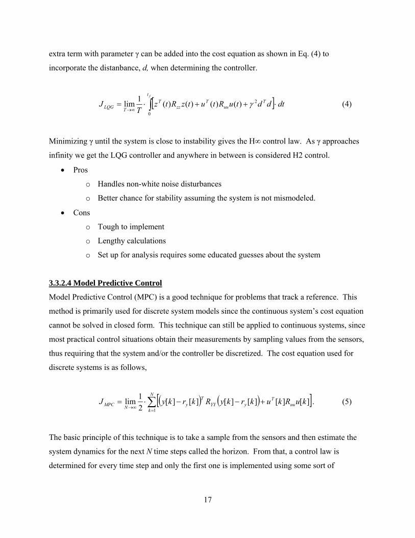
3.3.2.4 Model Predictive Control

Model Predictive Control (MPC) is a good technique for problems that track a reference. This

method is primarily used for discrete system models since the continuous system’s cost equation

cannot be solved in closed form. This technique can still be applied to continuous systems, since

most practical control situations obtain their measurements by sampling values from the sensors,

thus requiring that the system and/or the controller be discretized. The cost equation used for

discrete systems is as follows,

( ) ( )[ ]∑=

∞→+−−⋅=

N

kuu

TyYY

TyNMPC kuRkukrkyRkrkyJ

1

][][][][][][21lim . (5)

The basic principle of this technique is to take a sample from the sensors and then estimate the

system dynamics for the next N time steps called the horizon. From that, a control law is

determined for every time step and only the first one is implemented using some sort of

18

interpolation method. The process then repeats for the next time step. As the horizon increases,

the tracking tends to become more accurate.

• Pros

o Ideal for real time systems that are sampled.

o Simple to design once the system has be discretized.

• Cons

o Time consuming calculations to determine control for each sample.

o Minimum sampling period for stability may be higher than maximum attainable

sampling rate.

o Requires knowledge of the reference.

3.3.3. Controller Implementation Using the Mega32

There are a few big tradeoffs needed to determine the best way to implement the chosen

controller on the Mega32. It is necessary to consider the constraints imposed by the Mega32

before weighing the options of implementation. First off the Mega32 operates at 16MHz. Thus

if a high sample rate is chosen, the calculation time for state variables and the control effort may

be limited severely. Secondly, the on-board ADC has an execution speed of up to 15kHz per

conversion as discussed within the Feedback Network section which would limit the sampling

frequency of the sensors. Thirdly, there is only 32kB of flash memory for both the program and

variables, which would affect the amount of variables used for representing the state dynamics.

The first point necessary to consider is how fast should the sensors be sampled. There is the

trade-off between a high sampling rate which would limit the time for calculations and a low

sampling rate which would allow for more calculations between samples to implement the

control law. Analyzing this trade-off leads to the realization that if there is a lot of time for

calculations, by the time the control law is implemented, the actual system may have changed

drastically. Thus the control law would be ineffective. Though, if the sampling rate is too low,

there will not be enough time to calculate a control effort given any controller implementation.

Thus the best sampling rate will be the one that is as high as possible while still allowing enough

time to calculate a new control effort.

19

The next consideration is the method of calculations. Floating point allows for a full range of

control efforts, but unfortunately it takes a great deal of time which can further limit the

controller choices. Fixed point is less accurate, but has increased computation speed. The issue

with fixed point is that if there is a large range of values necessary for the design, it may make it

hard to develop a standard implementation. Thus the complexity of the code may increase

dramatically.

3.4. The Final Design Choices and Reasoning

3.4.1. The Final Design Choices

For this project, the U-channel track was chosen with a DC motor that has a sprocket attached to

its shaft to pull a chain. The control circuit is the H-bridge circuit designed for DC motors. The

cart is a block of wood mounted on matchbox cars with horizontal wheels on the bottom and top

to limit the degrees of freedom. The pendulum is mounted on the shaft on the angle measuring

circular potentiometer which is mounted on top of the cart. The position sensor is also a circular

potentiometer attached the drive sprocket. The sensors are sampled at the rate of the internal

ADC, but the values are only used to develop a control effort at a rate of 100Hz. This allows for

the most recent measurements to be available when it is necessary to determine a new control

effort. The actual controller was designed using LQR and is implemented using floating point

arithmetic.

3.4.2. The Reasoning Behind the Choices

The mechanical system was the most important subsystem of the design, which everything else

would need to be based off of. Thus the mechanical system needed to allow for easy

compatibility with the other subsystems. The U-channel seemed to offer this while still

maintaining the ability to actually work. It also would help restrict the degrees of freedom of the

cart making the cart design simpler. The friction might be a problem, but it should be possible to

model the friction and compensate for it using the controller. The U-channel also had the appeal

that the motor was a separate component that was not embedded in the cart. Thus if the motor

required any modifications, it could easily be removed and fixed. This system should be easier

to build which would reduce the chance for error due to the machine shop constraints. The

20

feedback network also was relatively easy to implement because of the U-channel. Circular

potentiometers would be simple to mount on both the cart and on the drive wheel.

The actual controller decision was based on the functionality of the Mega32. Obviously for a

MIMO system, a MIMO controller would be desired so classical control was ruled out. The

other control designs were complicated and required a large amount of floating point calculations

including matrix inversions for each sample. The LQR design provided the easiest

implementation with the minimum number of calculations, that would allow a high sampling

rate.

21

4. Design Process and It’s Implementation

Now that the basic design has been chosen, this section will discuss the actual design process.

Obviously there are many different components that need to be designed and built in order to get

this whole system up and running so the question is where to start? What makes this more

complicated is that most of the components are dependent upon each other. The answer to this

question, is the motor, which would probably be the limiting factor in the whole design (as well

as most expensive). Thus it is necessary to determine what constitutes a “good” motor and then

design the system around the motor such that the motor would be capable in controlling the cart

to keep the pendulum balanced. Detailed in the following section is the design process followed

for each subsystem and its final implementation.

4.1 Mechanical Parts

To design the mechanical subsystem, it was necessary to pick a “good” motor. As stated in the

The Range of Possible Solutions section, high speed and high torque are desirable for a fast and

accurate response, but what exactly is high speed and high torque? These questions could be

very hard to answer, but previous experience with this design problem in ECE 472 provided

valuable insight. Approximating, the cart would need to cover the length of the track in about 1

or 2 seconds and the torque had to be strong enough to overcome the forces exerted in the

horizontal direction by the track, cart, pendulum, and chain. Though at this point, the rest of the

system had not been designed so this would be hard to gauge. Fortunately, this problem has

been explored to exhaustion and there are many examples with typical parameters listed. From

these parameters, it would be easy to get an estimate of the forces in the horizontal direction. To

be conservative, all of the parameters were estimated in order to increase the minimum torque

needed to drive the system. This should help ensure that the motor would be capable of handling

a system with a smaller torque requirement.

To further gauge what constitutes a “good” motor, a motor was sampled from the ECE

department. A simple system could be built around this motor to see how well it could perform.

Conveniently the track was almost entirely independent of the motor. The largest factor in

determining a track was the length necessary for balancing the pendulum and a good size cross-

22

section such that cart would be wide enough and long enough to hold a pendulum. Using other

examples, the necessary track length could be estimated to be a couple meters long and have a

cross-section of approximately 5cm The actual U-channel track that met these measurements

was purchased from the physics department at Cornell University.

The mechanism that would pull cart turned out to be quite difficult to assemble. A bike chain

was chosen to pull the cart since this would be robust and very unlikely to slip and miss a step.

The bike chain, which was about 3 meters long (twice the length of the track), was purchased on

EBay. Sprockets were required to connect the bike chain to the motor shaft. These were

actually very difficult to find since the bike chain had a non-standard pitch-width of 35mm. One

thought would be to have a bike chain with a standard pitch-width. Unfortunately, it was hard to

find a chain with the standard pitch-width that was approximately 3 meters long.

After gathering all of these parts, a quick setup was assembled through the use of basic tools in

order to test the system. The cart was simple, built out of a block of wood with sliders typically

used for the bottom of furniture legs, and wheels designed for sliding screen doors. The cart was

attached to the chain using wood and screws that could fit within the chain loops. A simple test

program was written to move the cart back and forth with a set time interval for each direction.

The first trial run gave the indication from just observation that there may be enough speed, but

the torque was low. There was enough torque to pull the cart, but not enough to change

directions instantaneous, which would be necessary for implementing the control. Thus, a motor

with more torque is necessary even if it is at the cost of some speed. After searching and testing

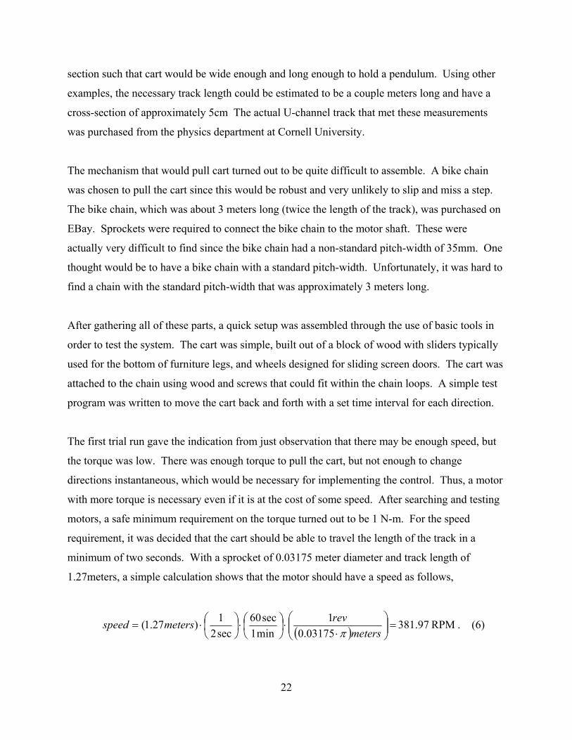
motors, a safe minimum requirement on the torque turned out to be 1 N-m. For the speed

requirement, it was decided that the cart should be able to travel the length of the track in a

minimum of two seconds. With a sprocket of 0.03175 meter diameter and track length of

1.27meters, a simple calculation shows that the motor should have a speed as follows,

( ) RPM 381.97 03175.0

1min1sec60

sec21)27.1( =⎟⎟

⎠

⎞⎜⎜⎝

⎛⋅

⋅⎟⎠⎞

⎜⎝⎛⋅⎟

⎠⎞

⎜⎝⎛⋅=

metersrevmetersspeedπ

. (6)

23

Thus the best motor found that was within budget turned out to have a torque of 1.356 N-m and a

speed of 330 RPM both measured without a load , operating at 24V, which had a current draw of

0.25A. This is close to the requirements determined above. Since the torque is high, it would be

possible to increase the drive sprocket size for more speed and less torque, if that turned out to be

necessary.

Once this motor was obtain, a new mechanical system needed to be developed. It was possible

to reuse the U-channel and bike chain used for the simple test system, but the sprocket had to be

fitted to this motor. For the free spinning wheel, a ball bearing assembly was purchased from a

bike store and the free-spinning sprocket was mounted to the ball bearing assembly in a similar

fashion. To actually mount the motor onto the track, a section of the track was cut such that the

motor could sit within the track while the chain and sprocket were outside the track. Holes were

drilled to hold both the motor and free-spinning assembly in place with screws.

For the final production of the cart, a smaller block of wood than the test system was chosen as

the base of the cart. To create the frictionless gliding motion, two identical matchbox cars were

mounted to the bottom using screws. This turned out to be a better alternative than either

attaching sliders (which still had a great deal of friction) or building a wheel assembly which

could cause a wobble in the cart. Horizontal wheels were also mounted on the top and bottom of

the cart to help limit the wobble in the cart. These wheels extended past the sides of the cart

almost reaching the inner sides of the track. One screw was mounted on either side of the cart

sticking straight up such that it would hit a mechanical switch that would disconnect the power

from the motor as a safety precaution if the cart traveled to the end of the track.

The pendulum was cut out of scrap aluminum in the shape of a rectangular prism with a hole

drilled near one end such that the pendulum could be mounted on the potentiometer.

Unfortunately this pendulum was not symmetric (though close) due to error from machining it.

The angle measuring potentiometer was mounted on the top of the cart near one side such that

the pendulum would be hanging off the side of the track opposite of the chain. A metal brace

was used to hold the potentiometer at the correct height with screws inserted in the brace to

restrict the potentiometer and pendulum from moving.

24

The mechanical switches, incorporated for safety concerns, were mounted onto blocks of wood

that would elevate the switches above the track such the switches were at the height of the cart

screws.

The track was also mounted onto two boards of wood, one on either side, to elevate the track off

the ground high enough such that the chain would not hit the ground.

Once the system was built, a controller was designed (as detailed in the next section).

Observation showed that the response of the system was too slow. To fix this, a larger sprocket

was inserted for the drive wheel which would decrease torque, but increase speed.

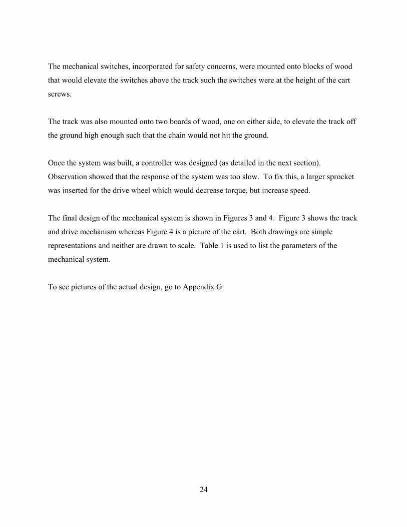
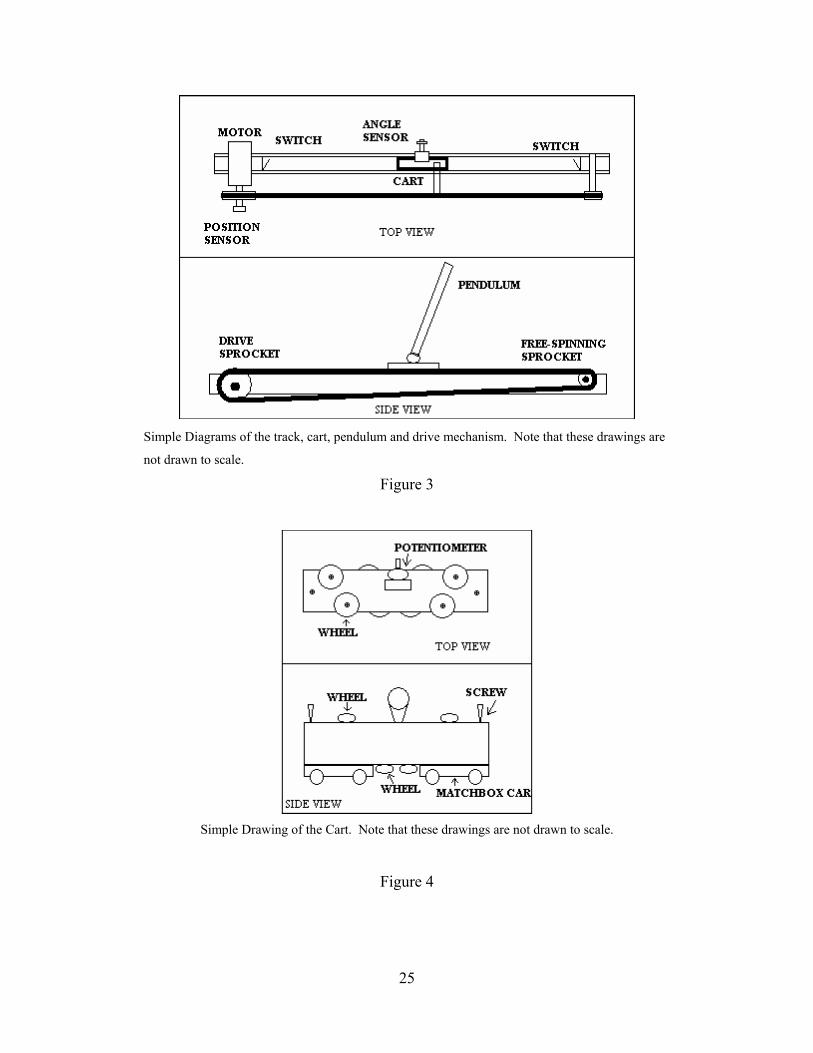
The final design of the mechanical system is shown in Figures 3 and 4. Figure 3 shows the track

and drive mechanism whereas Figure 4 is a picture of the cart. Both drawings are simple

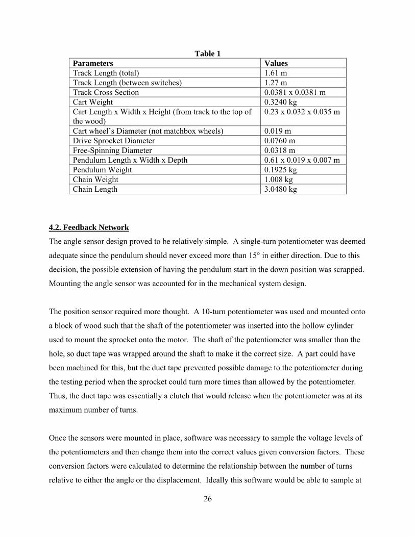
representations and neither are drawn to scale. Table 1 is used to list the parameters of the

mechanical system.

To see pictures of the actual design, go to Appendix G.

25

Simple Diagrams of the track, cart, pendulum and drive mechanism. Note that these drawings are

not drawn to scale.

Figure 3

Simple Drawing of the Cart. Note that these drawings are not drawn to scale.

Figure 4

26

Table 1 Parameters Values Track Length (total) 1.61 m Track Length (between switches) 1.27 m Track Cross Section 0.0381 x 0.0381 m Cart Weight 0.3240 kg Cart Length x Width x Height (from track to the top of the wood)

0.23 x 0.032 x 0.035 m

Cart wheel’s Diameter (not matchbox wheels) 0.019 m Drive Sprocket Diameter 0.0760 m Free-Spinning Diameter 0.0318 m Pendulum Length x Width x Depth 0.61 x 0.019 x 0.007 m Pendulum Weight 0.1925 kg Chain Weight 1.008 kg Chain Length 3.0480 kg

4.2. Feedback Network

The angle sensor design proved to be relatively simple. A single-turn potentiometer was deemed

adequate since the pendulum should never exceed more than 15° in either direction. Due to this

decision, the possible extension of having the pendulum start in the down position was scrapped.

Mounting the angle sensor was accounted for in the mechanical system design.

The position sensor required more thought. A 10-turn potentiometer was used and mounted onto

a block of wood such that the shaft of the potentiometer was inserted into the hollow cylinder

used to mount the sprocket onto the motor. The shaft of the potentiometer was smaller than the

hole, so duct tape was wrapped around the shaft to make it the correct size. A part could have

been machined for this, but the duct tape prevented possible damage to the potentiometer during

the testing period when the sprocket could turn more times than allowed by the potentiometer.

Thus, the duct tape was essentially a clutch that would release when the potentiometer was at its

maximum number of turns.

Once the sensors were mounted in place, software was necessary to sample the voltage levels of

the potentiometers and then change them into the correct values given conversion factors. These

conversion factors were calculated to determine the relationship between the number of turns

relative to either the angle or the displacement. Ideally this software would be able to sample at

27

a very high speed to give the most accurate measurements. For this system, the internal analog

to digital converter (ADC) of the Mega 32 was used for both measurements. The software

would continuously alternate between the two sensors and then exert a new control effort at a

frequency of 100Hz.

4.3. Control Circuit

The actual control circuit needed for this design is an H-bridge that can handle a couple Amps.

The motor draws 0.25A without a load so adding a load on with instant changes in direction will

create current levels of easily 3-4A. To implement the H-bride, the LMD18200 was sampled

from National Semiconductor. Following the application notes, the control circuit was built

using opto-isolators to connect the Mega32’s I/O ports to the LMD18200. This circuit was first

tested with a 50 V power source, which caused problems because there was too much power

across 0.125 Watt resistors causing them to burn out. Once a lab power supply of 20 V was

obtained, the circuit function correctly. A block diagram of the control circuit is shown in Figure

5. For the detailed schematic see Appendix A.

Block Diagram of the control circuit needed to drive the motor.

Figure5

4.4. System Model and Controller Design

Now that the mechanical subsystem is built and the feedback network is developed, it is possible

to design a controller. For the first attempt at designing a controller, the model was reduced such

28

that the system was linear. This used the assumptions that θ remained small and the moment of

inertia of the pendulum could be estimated to be zero. Due to these simplifications, the system

model became relatively simple. Using these simplified dynamics, an LQR controller was

developed. A Kalman Filter was also designed such that an LQG controller could be

implemented, but due to the number of floating point operations needed to actually implement

the Kalman Filter only the LQR solution could be used. The Mega 32 did not have enough

speed to process the observer while sampling the sensors at a reasonable rate. The error imposed

by the ADC and the tolerance of the potentiometers were relatively small (about a factor of 100

less) than the actual outputs, so it was not imperative to use a Kalman Filter.

Determining the “best” LQR solution required an iterative process of choosing weighting

matrices, developing a controller, and testing it. After many iterations, a controller was

developed that could balance the pendulum for a few seconds, though the displacement

performance suffered badly.

To improve the model, the moment of inertia of the pendulum was not assumed to be zero

anymore. This increased the complexity of the model, but stilled allowed for controller design

using what was a more accurate model. From this, an LQR controller was designed and tested

through the same iterative process as before until the “best” solution was determined. In this

case the pendulum balanced longer, though the displacement was still suffered.

4.4.1. The System Dynamics

Now that the design process is outlined, the final system model, state space representation and

controller design will now be described in detail. The actual design of the controller took a few

steps. First the system will need to be modeled with the desired assumptions such that the

system is linear and simple enough to design a controller for. From that, the model can then be

converted into state space form, which can then be used to design a controller using the LQR

cost equation.

29

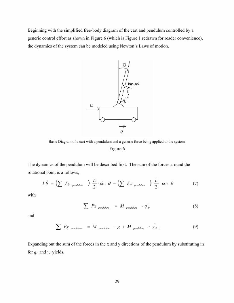
Beginning with the simplified free-body diagram of the cart and pendulum controlled by a

generic control effort as shown in Figure 6 (which is Figure 1 redrawn for reader convenience),

the dynamics of the system can be modeled using Newton’s Laws of motion.

Basic Diagram of a cart with a pendulum and a generic force being applied to the system.

Figure 6

The dynamics of the pendulum will be described first. The sum of the forces around the

rotational point is a follows,

( ) ( ) θθθ cos2

sin2

..⋅⋅−⋅⋅= ∑∑ LFxLFyI pendulumpendulum (7)

with

∑ ⋅=..

Ppendulumpendulum qMFx (8)

and ..

Ppendulumpendulumpendulum yMgMFy ⋅+⋅=∑ . (9)

Expanding out the sum of the forces in the x and y directions of the pendulum by substituting in

for qP and yP yields,

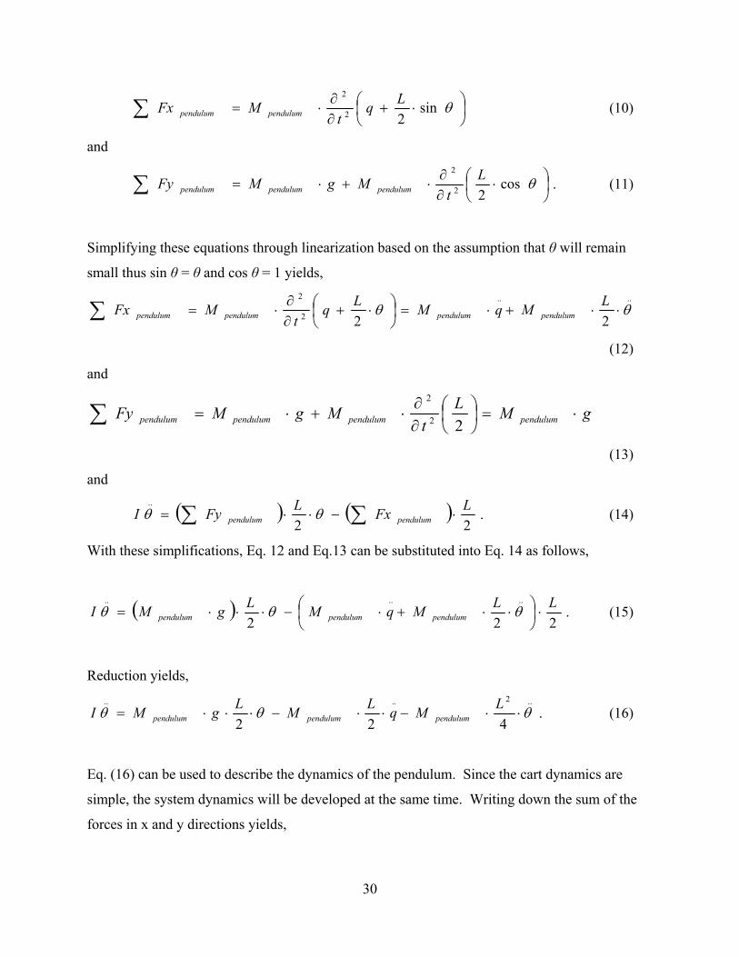
30

⎟⎠⎞

⎜⎝⎛ ⋅+

∂∂

⋅=∑ θsin22

2 Lqt

MFx pendulumpendulum (10)

and

⎟⎠⎞

⎜⎝⎛ ⋅

∂∂

⋅+⋅=∑ θcos22

2 Lt

MgMFy pendulumpendulumpendulum . (11)

Simplifying these equations through linearization based on the assumption that θ will remain

small thus sin θ = θ and cos θ = 1 yields,

....

2

2

22θθ ⋅⋅+⋅=⎟

⎠⎞

⎜⎝⎛ ⋅+

∂∂

⋅=∑ LMqMLqt

MFx pendulumpendulumpendulumpendulum

(12)

and

gMLt

MgMFy pendulumpendulumpendulumpendulum ⋅=⎟⎠⎞

⎜⎝⎛

∂∂

⋅+⋅=∑ 22

2

(13)

and

( ) ( )22

.. LFxLFyI pendulumpendulum ⋅−⋅⋅= ∑∑ θθ . (14)

With these simplifications, Eq. 12 and Eq.13 can be substituted into Eq. 14 as follows,

( )222

...... LLMqMLgMI pendulumpendulumpendulum ⋅⎟⎠⎞

⎜⎝⎛ ⋅⋅+⋅−⋅⋅⋅= θθθ . (15)

Reduction yields,

..2....

422θθθ ⋅⋅−⋅⋅−⋅⋅⋅=

LMqLMLgMI pendulumpendulumpendulum . (16)

Eq. (16) can be used to describe the dynamics of the pendulum. Since the cart dynamics are

simple, the system dynamics will be developed at the same time. Writing down the sum of the

forces in x and y directions yields,

31

∑∑ +−⋅+⋅= pendulumcartchaincart FxuqMqMFx....

(17)

and

0=∑ cartFy . (18)

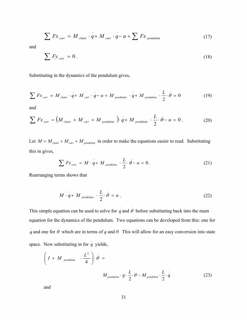
Substituting in the dynamics of the pendulum gives,

02

........=⋅⋅+⋅+−⋅+⋅=∑ θLMqMuqMqMFx pendulumpendulumcartchaincart (19)

and

( ) 02

....=−⋅⋅+⋅++=∑ uLMqMMMFx pendulumpendulumcartchaincart θ . (20)

Let pendulumcartchain MMMM ++= in order to make the equations easier to read. Substituting

this in gives,

02

....=−⋅⋅+⋅=∑ uLMqMFx pendulumcart θ . (21)

Rearranging terms shows that

uLMqM pendulum =⋅⋅+⋅....

2θ . (22)

This simple equation can be used to solve for ..q and

..θ before substituting back into the main

equation for the dynamics of the pendulum. Two equations can be developed from this: one for ..q and one for

..θ which are in terms of q and θ. This will allow for an easy conversion into state

space. Now substituting in for ..q yields,

=⋅⎟⎟⎠

⎞⎜⎜⎝

⎛⋅+

..2

4θLMI pendulum

..

22qLMLgM pendulumpendulum ⋅⋅−⋅⋅⋅ θ (23)

and

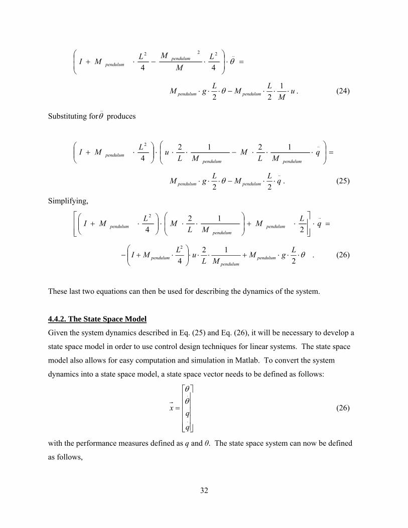
32

=⋅⎟⎟⎠

⎞⎜⎜⎝

⎛⋅−⋅+

..222

44θL

MMLMI pendulum

pendulum

uM

LMLgM pendulumpendulum ⋅⋅⋅−⋅⋅⋅1

22θ . (24)

Substituting for..θ produces

=⎟⎟⎠

⎞⎜⎜⎝

⎛⋅⋅⋅−⋅⋅⋅⎟⎟

⎠

⎞⎜⎜⎝

⎛⋅+

..2 12124

qML

MML

uLMIpendulumpendulum

pendulum

..

22qLMLgM pendulumpendulum ⋅⋅−⋅⋅⋅ θ . (25)

Simplifying,

=⋅⎥⎥⎦

⎤

⎢⎢⎣

⎡⋅+⎟

⎟⎠

⎞⎜⎜⎝

⎛⋅⋅⋅⎟⎟

⎠

⎞⎜⎜⎝

⎛⋅+

..2

212

4qLM

MLMLMI pendulum

pendulumpendulum

θ⋅⋅⋅+⋅⋅⋅⎟⎟⎠

⎞⎜⎜⎝

⎛⋅+−

212

4

2 LgMML

uLMI pendulumpendulum

pendulum . (26)

These last two equations can then be used for describing the dynamics of the system.

4.4.2. The State Space Model

Given the system dynamics described in Eq. (25) and Eq. (26), it will be necessary to develop a

state space model in order to use control design techniques for linear systems. The state space

model also allows for easy computation and simulation in Matlab. To convert the system

dynamics into a state space model, a state space vector needs to be defined as follows:

⎥⎥⎥⎥⎥

⎦

⎤

⎢⎢⎢⎢⎢

⎣

⎡

=.

.

q

qx

θθ

(26)

with the performance measures defined as q and θ. The state space system can now be defined

as follows,

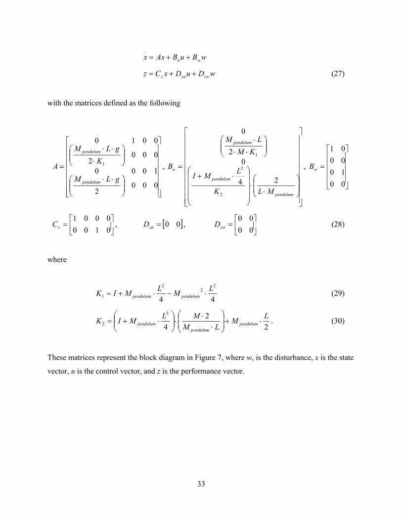
33

wBuBAxx wu ++=.

wDuDxCz zwzuz ++= (27)

with the matrices defined as the following

⎥⎥⎥⎥⎥⎥⎥

⎦

⎤

⎢⎢⎢⎢⎢⎢⎢

⎣

⎡

⎟⎟⎠

⎞⎜⎜⎝

⎛ ⋅⋅

⎟⎟⎠

⎞⎜⎜⎝

⎛⋅

⋅⋅

=

0002

1000

0002

0010

1

gLM

KgLM

A

pendulum

pendulum

,

⎥⎥⎥⎥⎥⎥⎥⎥⎥

⎦

⎤

⎢⎢⎢⎢⎢⎢⎢⎢⎢

⎣

⎡

⎟⎟⎠

⎞⎜⎜⎝

⎛

⋅⋅

⎟⎟⎟⎟

⎠

⎞

⎜⎜⎜⎜

⎝

⎛⋅+

⎟⎟⎠

⎞⎜⎜⎝

⎛⋅⋅

⋅

=

pendulum

pendulum

pendulum

u

MLK

LMI

KMLM

B

24

02

0

2

2

1

,

⎥⎥⎥⎥

⎦

⎤

⎢⎢⎢⎢

⎣

⎡

=

00100001

wB

⎥⎦

⎤⎢⎣

⎡=

01000001

zC , [ ]00=zuD , ⎥⎦

⎤⎢⎣

⎡=

0000

zwD (28)

where

44

22

2

1LMLMIK pendulumpendulum ⋅−⋅+= (29)

22

4

2

2LM

LMMLMIK pendulum

pendulumpendulum ⋅+⎟

⎟⎠

⎞⎜⎜⎝

⎛

⋅⋅

⋅⎟⎟⎠

⎞⎜⎜⎝

⎛⋅+= . (30)

These matrices represent the block diagram in Figure 7, where w, is the disturbance, x is the state

vector, u is the control vector, and z is the performance vector.

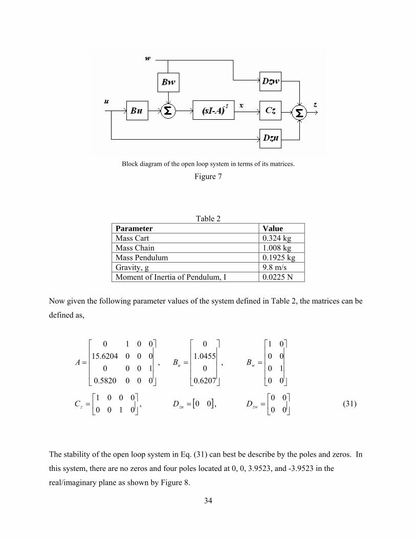
34

Block diagram of the open loop system in terms of its matrices.

Figure 7

Table 2 Parameter Value Mass Cart 0.324 kg Mass Chain 1.008 kg Mass Pendulum 0.1925 kg Gravity, g 9.8 m/s Moment of Inertia of Pendulum, I 0.0225 N

Now given the following parameter values of the system defined in Table 2, the matrices can be

defined as,

⎥⎥⎥⎥

⎦

⎤

⎢⎢⎢⎢

⎣

⎡

=

0005820.010000006204.150010

A ,

⎥⎥⎥⎥

⎦

⎤

⎢⎢⎢⎢

⎣

⎡

=

6207.00

0455.10

uB ,

⎥⎥⎥⎥

⎦

⎤

⎢⎢⎢⎢

⎣

⎡

=

00100001

wB

⎥⎦

⎤⎢⎣

⎡=

01000001

zC , [ ]00=zuD , ⎥⎦

⎤⎢⎣

⎡=

0000

zwD (31)

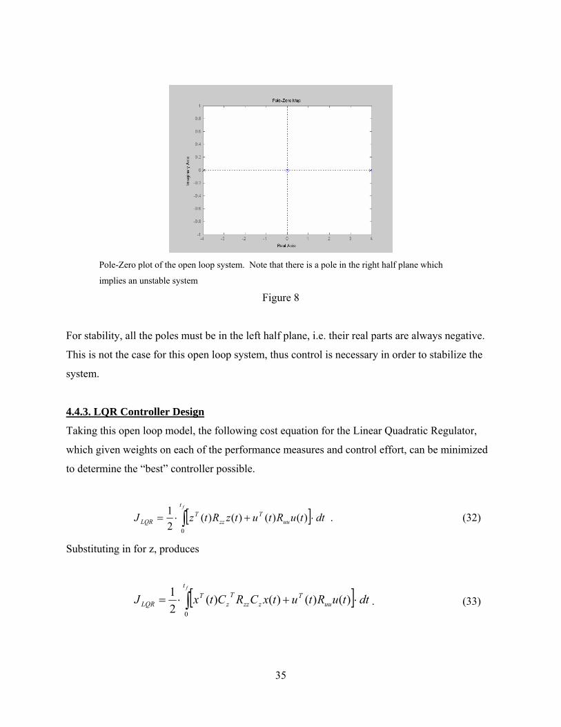
The stability of the open loop system in Eq. (31) can best be describe by the poles and zeros. In

this system, there are no zeros and four poles located at 0, 0, 3.9523, and -3.9523 in the

real/imaginary plane as shown by Figure 8.

35

Pole-Zero plot of the open loop system. Note that there is a pole in the right half plane which

implies an unstable system

Figure 8

For stability, all the poles must be in the left half plane, i.e. their real parts are always negative.

This is not the case for this open loop system, thus control is necessary in order to stabilize the

system.

4.4.3. LQR Controller Design

Taking this open loop model, the following cost equation for the Linear Quadratic Regulator,

which given weights on each of the performance measures and control effort, can be minimized

to determine the “best” controller possible.

[ ]∫ ⋅+⋅=ft

uuT

zzT

LQR dttuRtutzRtzJ0

)()()()(21 . (32)

Substituting in for z, produces

[ ]∫ ⋅+⋅=ft

uuT

zzzT

zT

LQR dttuRtutxCRCtxJ0

)()()()(21

. (33)

36

Rewriting with zzzT

z CRCQ = gives

[ ]∫ ⋅+⋅=ft

uuTT

LQR dttuRtutQxtxJ0

)()()()(21 . (34)

The derivation of the solution to minimizing this cost equation involves Lagrange multipliers and

is done in most multivariable control textbooks. This derivation will not be done here, but the

end result will be used obtained from lectures notes for MAE 678. Eq. (35) represents the

Algebraic Riccati Equation which will produce the solution to the Stochastic LQR.

T

uuuuT BRSBSASAQ 10 −+−−−= (35)

where S and Q are positive semi-definite and S is also symmetric. For this project, after a great

deal of experimentation, Bryson’s Rule was used to determine the weights of Rzz and Ruu.

Bryon’s Rule, as stated earlier, says for each performance variable and the control effort to take

inverse of the squared maximum desired value. This turns out to be a good starting point with

which to then make minor adjustments until the optimal output is achieved. The final weighting

matrices were chosen as follows,

⎥⎥⎥

⎦

⎤

⎢⎢⎢

⎣

⎡

=

2

2

68.010

00183.0

1

zzR , 231

=uuR (36)

where the first entry of Rzz is in radians per second for the maximum angle desired and the

second entry is in meters for the maximum displacement. Ruu is in Newtons.

Now solving the Algebraic Riccati Equation for S using the above values, produces

37

⎥⎥⎥⎥

⎦

⎤

⎢⎢⎢⎢

⎣

⎡

−−−−

−−−−

=

9324.43327.37515.35683.113327.37967.34475.29835.77515.34475.29581.37360.145683.119835.77360.143298.74

S (37)

Given S, the control matrix can be defined as,

SBRF Tuuu

1−−= . (38)

This gives

[ ]7452.74118.42864.160346.74 −−=F (39)

With this control matrix, a control law can be defined as

Fxu −= . (40)

This can then be substituted back into the system equations defined in Eq. (27) to give,

( ) wBFxBAxx wu +−+=.

wDuDxCz zwzuz ++= (41)

Given that Dzu and Dzw both have only zero entries and rearranging some terms, Eq. (41) can be

simplified to

( ) wBxFBAx wu +−=.

xCz z= (42)

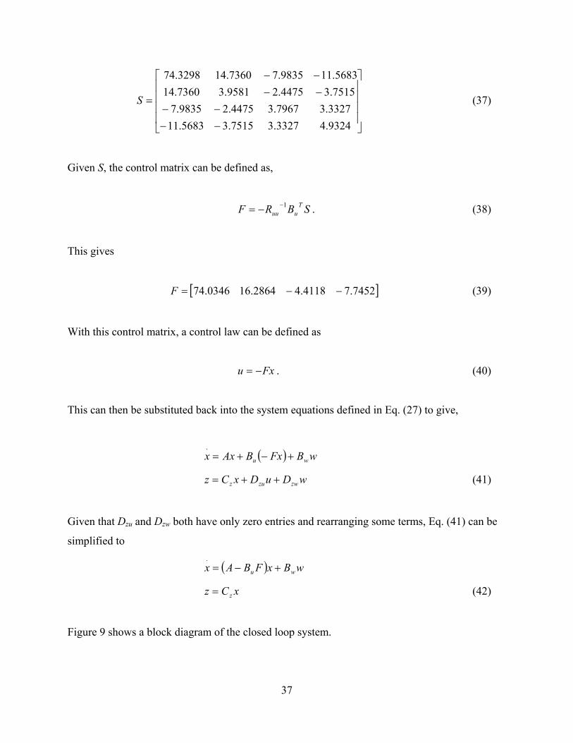
Figure 9 shows a block diagram of the closed loop system.

38

Block diagram of the closed loop system in terms of its matrices.

Figure 9

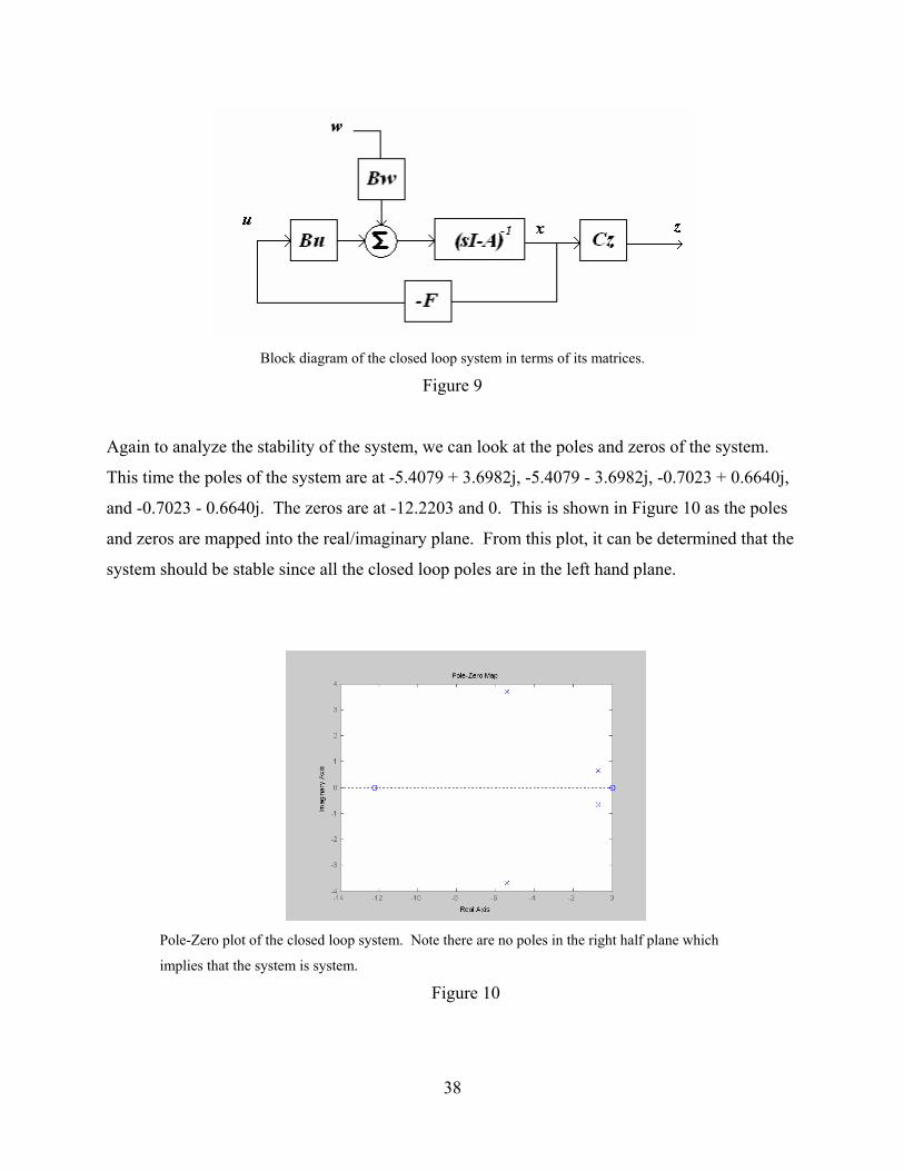
Again to analyze the stability of the system, we can look at the poles and zeros of the system.

This time the poles of the system are at -5.4079 + 3.6982j, -5.4079 - 3.6982j, -0.7023 + 0.6640j,

and -0.7023 - 0.6640j. The zeros are at -12.2203 and 0. This is shown in Figure 10 as the poles

and zeros are mapped into the real/imaginary plane. From this plot, it can be determined that the

system should be stable since all the closed loop poles are in the left hand plane.

Pole-Zero plot of the closed loop system. Note there are no poles in the right half plane which

implies that the system is system.

Figure 10

39

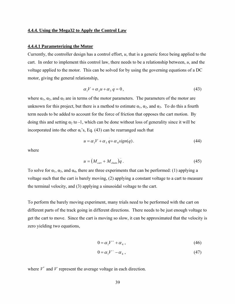
4.4.4. Using the Mega32 to Apply the Control Law

4.4.4.1 Parameterizing the Motor

Currently, the controller design has a control effort, u, that is a generic force being applied to the

cart. In order to implement this control law, there needs to be a relationship between, u, and the

voltage applied to the motor. This can be solved for by using the governing equations of a DC

motor, giving the general relationship,

0.

321 =++ quV ααα , (43)

where α1, α2, and α3 are in terms of the motor parameters. The parameters of the motor are

unknown for this project, but there is a method to estimate α1, α2, and α3. To do this a fourth

term needs to be added to account for the force of friction that opposes the cart motion. By

doing this and setting α2 to -1, which can be done without loss of generality since it will be

incorporated into the other αi’s, Eq. (43) can be rearranged such that

)(.

4

.

31 qsignqVu ααα ++= . (44)

where

( )..qMMu chaincart += . (45)

To solve for α1, α3, and α4, there are three experiments that can be performed: (1) applying a

voltage such that the cart is barely moving, (2) applying a constant voltage to a cart to measure

the terminal velocity, and (3) applying a sinusoidal voltage to the cart.

To perform the barely moving experiment, many trials need to be performed with the cart on

different parts of the track going in different directions. There needs to be just enough voltage to

get the cart to move. Since the cart is moving so slow, it can be approximated that the velocity is

zero yielding two equations,

410 αα += +V , (46)

410 αα −= −V , (47)

where V+ and V- represent the average voltage in each direction.

40

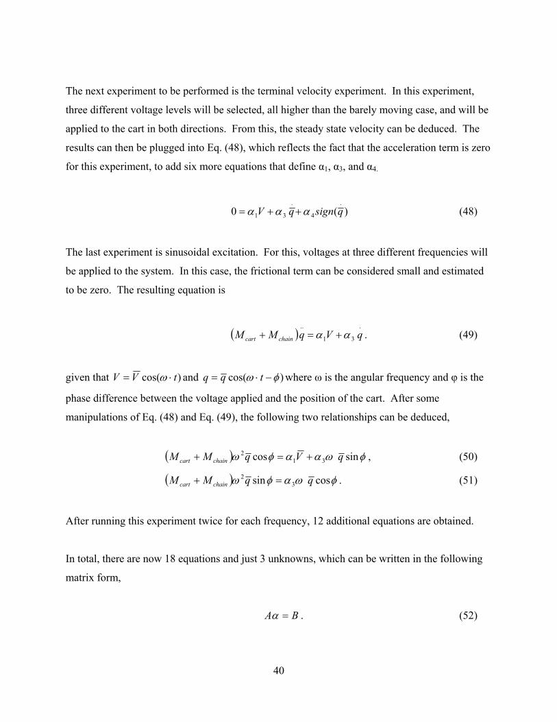
The next experiment to be performed is the terminal velocity experiment. In this experiment,

three different voltage levels will be selected, all higher than the barely moving case, and will be

applied to the cart in both directions. From this, the steady state velocity can be deduced. The

results can then be plugged into Eq. (48), which reflects the fact that the acceleration term is zero

for this experiment, to add six more equations that define α1, α3, and α4.

)(0.

4

.

31 qsignqV ααα ++= (48)

The last experiment is sinusoidal excitation. For this, voltages at three different frequencies will

be applied to the system. In this case, the frictional term can be considered small and estimated

to be zero. The resulting equation is

( ).

31

..qVqMM chaincart αα +=+ . (49)

given that )cos( tVV ⋅= ω and )cos( φω −⋅= tqq where ω is the angular frequency and φ is the

phase difference between the voltage applied and the position of the cart. After some

manipulations of Eq. (48) and Eq. (49), the following two relationships can be deduced,

( ) φωααφω sincos 312 qVqMM chaincart +=+ , (50)

( ) φωαφω cossin 32 qqMM chaincart =+ . (51)

After running this experiment twice for each frequency, 12 additional equations are obtained.

In total, there are now 18 equations and just 3 unknowns, which can be written in the following

matrix form,

BA =α . (52)

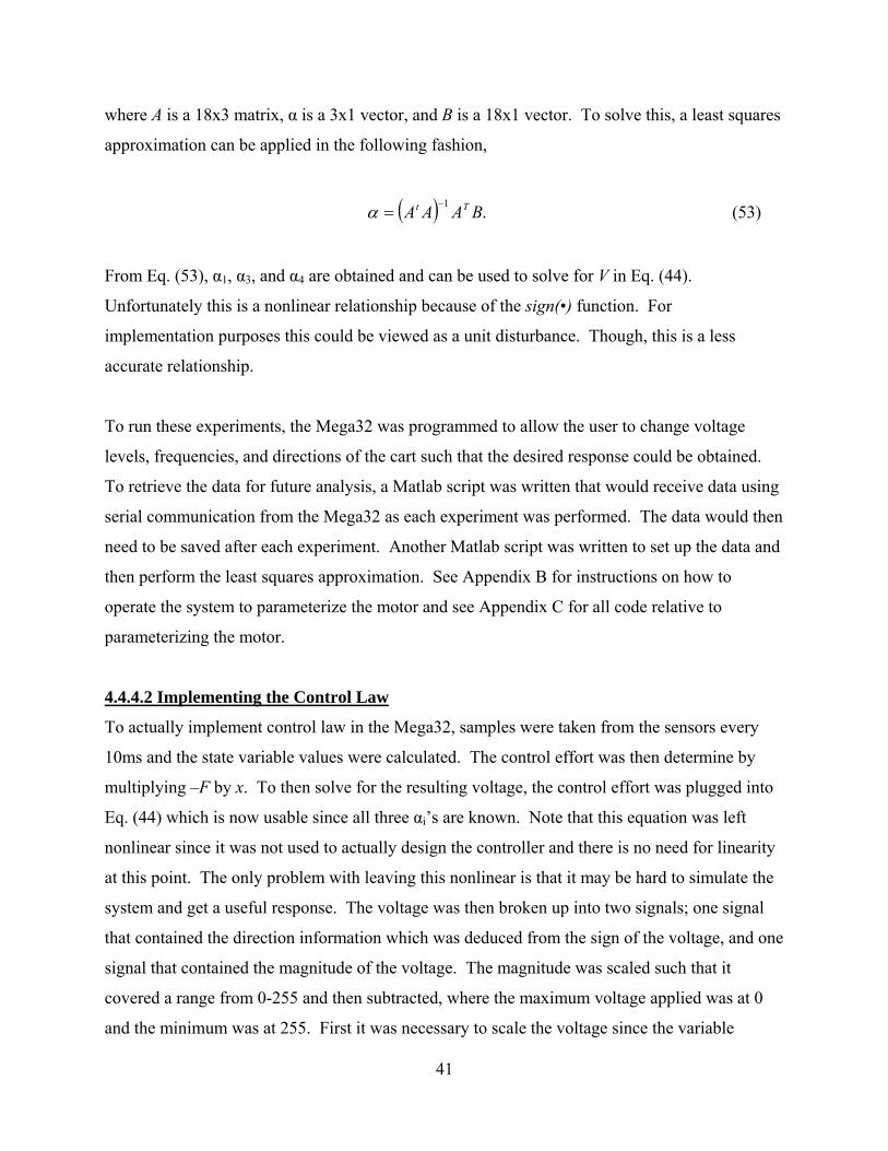
41

where A is a 18x3 matrix, α is a 3x1 vector, and B is a 18x1 vector. To solve this, a least squares

approximation can be applied in the following fashion,

( ) .1 BAAA Tt −=α (53)

From Eq. (53), α1, α3, and α4 are obtained and can be used to solve for V in Eq. (44).

Unfortunately this is a nonlinear relationship because of the sign(•) function. For

implementation purposes this could be viewed as a unit disturbance. Though, this is a less

accurate relationship.

To run these experiments, the Mega32 was programmed to allow the user to change voltage

levels, frequencies, and directions of the cart such that the desired response could be obtained.

To retrieve the data for future analysis, a Matlab script was written that would receive data using

serial communication from the Mega32 as each experiment was performed. The data would then

need to be saved after each experiment. Another Matlab script was written to set up the data and

then perform the least squares approximation. See Appendix B for instructions on how to

operate the system to parameterize the motor and see Appendix C for all code relative to

parameterizing the motor.

4.4.4.2 Implementing the Control Law

To actually implement control law in the Mega32, samples were taken from the sensors every

10ms and the state variable values were calculated. The control effort was then determine by

multiplying –F by x. To then solve for the resulting voltage, the control effort was plugged into

Eq. (44) which is now usable since all three αi’s are known. Note that this equation was left

nonlinear since it was not used to actually design the controller and there is no need for linearity

at this point. The only problem with leaving this nonlinear is that it may be hard to simulate the

system and get a useful response. The voltage was then broken up into two signals; one signal

that contained the direction information which was deduced from the sign of the voltage, and one

signal that contained the magnitude of the voltage. The magnitude was scaled such that it

covered a range from 0-255 and then subtracted, where the maximum voltage applied was at 0

and the minimum was at 255. First it was necessary to scale the voltage since the variable

42

holding the voltage level could take on all 255 possible values, thus this would allow for more

fine tuning. The magnitude was subtracted from 255 since the opto-isolator circuit would invert

the actual signal. There is one problem with the second signal- it requires an analog output,

while the Mega32 has purely digital I/O ports. One solution, would be to use the Pulse Width

Modulator (PWM) such that if it is operating at high speeds, the output signal appears to be the

average voltage of the PWM which is proportional to the duty cycle. The final source code for

implementing a controller can be found in Appendix E whereas the actual controller design code

is found in Appendix D.

4.5. Evolution of the Requirements

Through this design process, the requirements evolved due to multiple set backs including three

broken motors, and difficulty implementing a working controller. Because of these problems,

the requirements were stripped down to the basic solution to the problem stated above. A lot of

the requirements discussed in Section 2.3 could be implemented relatively easy given more time.

The final requirements are as follows:

• Decently designed sensors.

• Matlab interface (data extraction only).

• Programmable to allow for multiple solutions (less structured).

• Main solution balances for a few seconds. Limitations in parts, hardware, and software

prevent better solutions.

43

5. Results Compared to Expectations

First off, the cart was able to balance the pendulum for about 3-5 seconds completely on its own

before getting to close to the edge of the track. As the cart approached the edge of the track, a

small “tap” on the pendulum in the other direction, would allow the cart to balance the pendulum

longer. The inability to balance a pendulum for an extended period of time can possibly be

attributed to many different factors. First of all, implementing just the LQR solution was due to

the fact that floating arithmetic was used on the Mega32 to calculate the control law. If fixed

point had been implemented, there might have a been a chance to implement a full LQG

controller or possibly an MPC controller. Though a fixed point implementation might not have

been feasible since there was a large range of values necessary to represent the parameters.

Given more time, a clever implementation could be deduced. Another factor that could be

limiting the success of the design is the model of the system. Since the system is quite complex

mechanically, there are many parts that interact with each other which could lead to mismodeled

and unmodeled dynamics. The system also has many imperfections such as the pendulum is not

completely constrained to just two degrees of freedom. Another factor that could cause some

error is that the sampling rate is slow enough that it may not be possible to implement a working

controller using a continuous time design. A few discrete controllers were designed and tested,

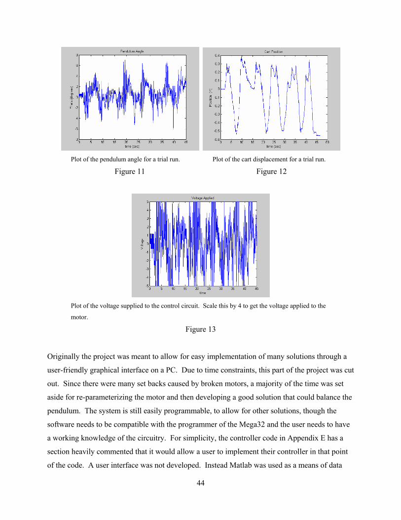
but all of them failed to show any promise. Figures 11 and 12 are plots of the angle and

displacement measurements as a function of time, which were taken from a trial run of balancing

the pendulum with occasional “taps” applied to the pendulum whenever the cart was close to the

edge of the track. Figure 13 shows the average voltage applied by the MCU to the control

circuit. This can be scaled to determine the voltage applied to the motor given the maximum

voltage of the motor power supply.

44

Plot of the pendulum angle for a trial run. Plot of the cart displacement for a trial run.

Figure 11 Figure 12

Plot of the voltage supplied to the control circuit. Scale this by 4 to get the voltage applied to the

motor.

Figure 13

Originally the project was meant to allow for easy implementation of many solutions through a

user-friendly graphical interface on a PC. Due to time constraints, this part of the project was cut

out. Since there were many set backs caused by broken motors, a majority of the time was set

aside for re-parameterizing the motor and then developing a good solution that could balance the

pendulum. The system is still easily programmable, to allow for other solutions, though the

software needs to be compatible with the programmer of the Mega32 and the user needs to have

a working knowledge of the circuitry. For simplicity, the controller code in Appendix E has a

section heavily commented that it would allow a user to implement their controller in that point

of the code. A user interface was not developed. Instead Matlab was used as a means of data

45

extraction and parameter calculations. The system is actually self-contained once the Mega32 is

programmed, though to record data, the system needs to be hooked up to a PC with the Matlab

script used for data extraction.

46

6. Conclusion

Overall the project can be considered a success. Despite the fact that the main goal of the project

was not reached- the cart was unable to balance the pendulum for an extended period of time- the

foundation is laid for future research. Many requirements were met such that a working

mechanical system was developed along with a control circuit and an accurate feedback network.

An interface was also created through hardware and software to integrate the Mega32 as the

main processing unit for the controller. From this, it seems that with the right modifications, it

would be quite feasible to balance a pendulum for an extended period of time. The system

would need to modified to reduce some of the imperfections and increase the torque and speed of

the motor. A variety of control designs could be implemented using some of the other suggested

methods in this report.

The most beneficial aspect of this project was that it gave exposure to a full system design. The

experience gained from developing each of the subsystems given the constraints they imposed on

each other and then integrating them together proved to be invaluable.

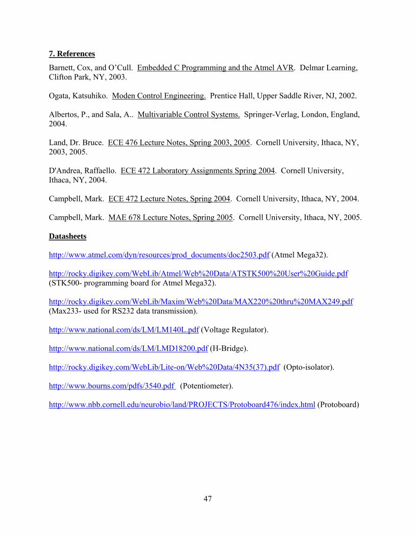
47

7. References

Barnett, Cox, and O’Cull. Embedded C Programming and the Atmel AVR. Delmar Learning, Clifton Park, NY, 2003. Ogata, Katsuhiko. Moden Control Engineering. Prentice Hall, Upper Saddle River, NJ, 2002. Albertos, P., and Sala, A.. Multivariable Control Systems. Springer-Verlag, London, England, 2004. Land, Dr. Bruce. ECE 476 Lecture Notes, Spring 2003, 2005. Cornell University, Ithaca, NY, 2003, 2005. D'Andrea, Raffaello. ECE 472 Laboratory Assignments Spring 2004. Cornell University, Ithaca, NY, 2004. Campbell, Mark. ECE 472 Lecture Notes, Spring 2004. Cornell University, Ithaca, NY, 2004. Campbell, Mark. MAE 678 Lecture Notes, Spring 2005. Cornell University, Ithaca, NY, 2005. Datasheets

http://www.atmel.com/dyn/resources/prod_documents/doc2503.pdf (Atmel Mega32).

http://rocky.digikey.com/WebLib/Atmel/Web%20Data/ATSTK500%20User%20Guide.pdf (STK500- programming board for Atmel Mega32).

http://rocky.digikey.com/WebLib/Maxim/Web%20Data/MAX220%20thru%20MAX249.pdf (Max233- used for RS232 data transmission).

http://www.national.com/ds/LM/LM140L.pdf (Voltage Regulator).

http://www.national.com/ds/LM/LMD18200.pdf (H-Bridge).

http://rocky.digikey.com/WebLib/Lite-on/Web%20Data/4N35(37).pdf (Opto-isolator).

http://www.bourns.com/pdfs/3540.pdf (Potentiometer). http://www.nbb.cornell.edu/neurobio/land/PROJECTS/Protoboard476/index.html (Protoboard)

48

8. Acknowledgements

I would like to thank…

• … my advisor, Dr. Bruce Land for his help and guidance throughout the whole process.

• … my peer and high school friend Kyle McMann for his time and help machining some

of the intricate parts of the mechanical system.

• … my Dad, Lyle Stang, for his help attaching the drive mechanism (motor, sprockets and

chain) to the track as well as his help with designing a cart.

• … Gary Oltz for his help with machining the track and drive mechanism for the first

version of this design.

• … Dr. John Belina and Bill Mutch for supplying a sample motor and 20V power source

needed for this design project.

49

Appendix A: Schematics

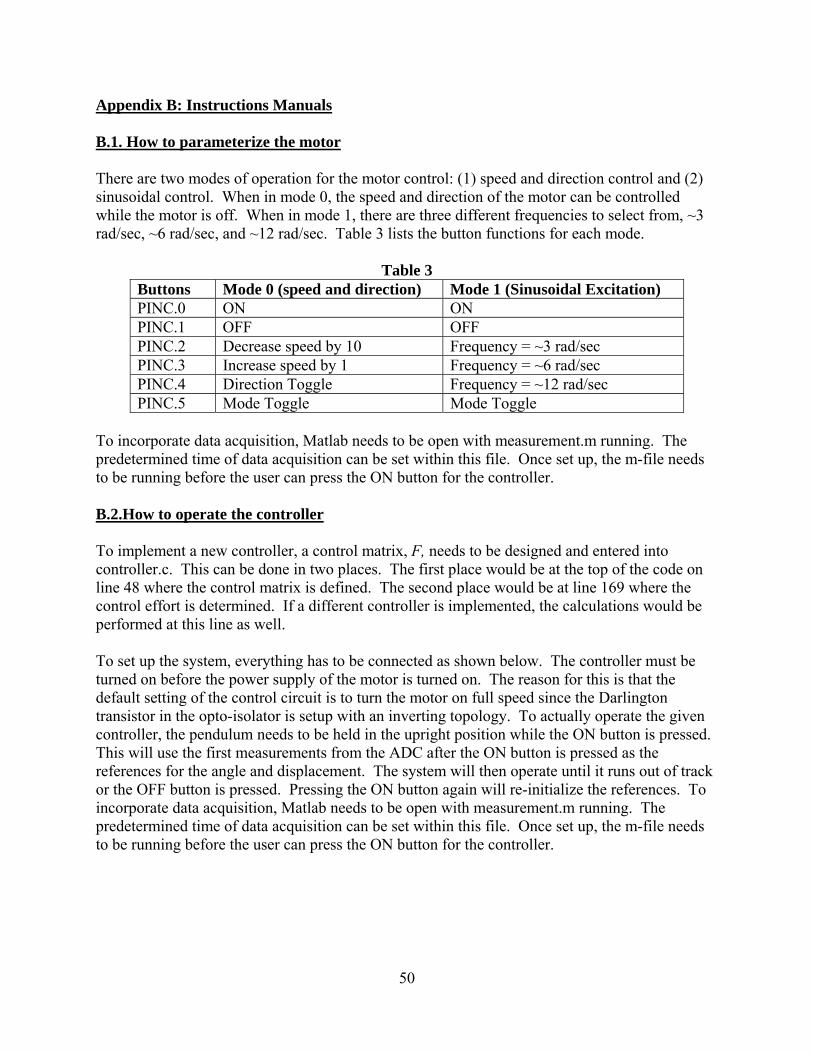
50

Appendix B: Instructions Manuals B.1. How to parameterize the motor There are two modes of operation for the motor control: (1) speed and direction control and (2) sinusoidal control. When in mode 0, the speed and direction of the motor can be controlled while the motor is off. When in mode 1, there are three different frequencies to select from, ~3 rad/sec, ~6 rad/sec, and ~12 rad/sec. Table 3 lists the button functions for each mode.

Table 3 Buttons Mode 0 (speed and direction) Mode 1 (Sinusoidal Excitation) PINC.0 ON ON PINC.1 OFF OFF PINC.2 Decrease speed by 10 Frequency = ~3 rad/sec PINC.3 Increase speed by 1 Frequency = ~6 rad/sec PINC.4 Direction Toggle Frequency = ~12 rad/sec PINC.5 Mode Toggle Mode Toggle

To incorporate data acquisition, Matlab needs to be open with measurement.m running. The predetermined time of data acquisition can be set within this file. Once set up, the m-file needs to be running before the user can press the ON button for the controller. B.2.How to operate the controller To implement a new controller, a control matrix, F, needs to be designed and entered into controller.c. This can be done in two places. The first place would be at the top of the code on line 48 where the control matrix is defined. The second place would be at line 169 where the control effort is determined. If a different controller is implemented, the calculations would be performed at this line as well. To set up the system, everything has to be connected as shown below. The controller must be turned on before the power supply of the motor is turned on. The reason for this is that the default setting of the control circuit is to turn the motor on full speed since the Darlington transistor in the opto-isolator is setup with an inverting topology. To actually operate the given controller, the pendulum needs to be held in the upright position while the ON button is pressed. This will use the first measurements from the ADC after the ON button is pressed as the references for the angle and displacement. The system will then operate until it runs out of track or the OFF button is pressed. Pressing the ON button again will re-initialize the references. To incorporate data acquisition, Matlab needs to be open with measurement.m running. The predetermined time of data acquisition can be set within this file. Once set up, the m-file needs to be running before the user can press the ON button for the controller.

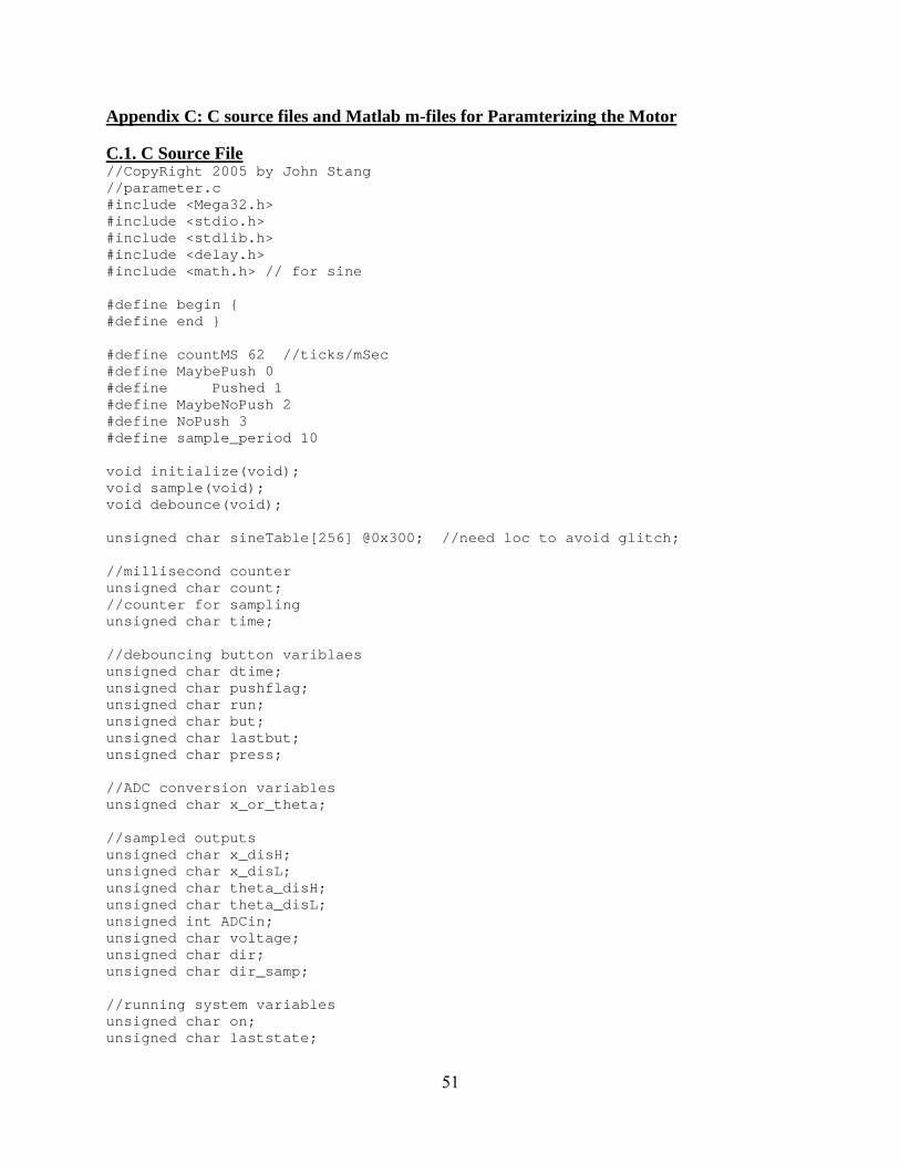
51

Appendix C: C source files and Matlab m-files for Paramterizing the Motor C.1. C Source File //CopyRight 2005 by John Stang //parameter.c #include <Mega32.h> #include <stdio.h> #include <stdlib.h> #include <delay.h> #include <math.h> // for sine #define begin { #define end } #define countMS 62 //ticks/mSec #define MaybePush 0 #define Pushed 1 #define MaybeNoPush 2 #define NoPush 3 #define sample_period 10 void initialize(void); void sample(void); void debounce(void); unsigned char sineTable[256] @0x300; //need loc to avoid glitch; //millisecond counter unsigned char count; //counter for sampling unsigned char time; //debouncing button variblaes unsigned char dtime; unsigned char pushflag; unsigned char run; unsigned char but; unsigned char lastbut; unsigned char press; //ADC conversion variables unsigned char x_or_theta; //sampled outputs unsigned char x_disH; unsigned char x_disL; unsigned char theta_disH; unsigned char theta_disL; unsigned int ADCin; unsigned char voltage; unsigned char dir; unsigned char dir_samp; //running system variables unsigned char on; unsigned char laststate;

52

//sinusoidal tests unsigned int freq[3] = {8,4,2}; unsigned int sin_count; unsigned char sin_test; unsigned char freq_count; unsigned char index; unsigned int i; unsigned int speed; unsigned int debounce2; unsigned char mode; //Interrupt used to set up time base interrupt [TIM0_OVF] void sgen(void) begin //generate rising amplitude // 62 counts is about 1 mSec count--; if (0 == count ) begin count=countMS; time++; dtime++; sin_count++; debounce2++; end//end millisecond timer //sinusoidal output if (sin_test ==1) begin PORTB =~OCR1A; if (sin_count == freq[freq_count]) begin sin_count = 0; OCR1A = sineTable[index++]; if (index == 128) begin PORTD.4 = 0; dir = 0; end else begin if (index ==255) begin PORTD.4 = 1; dir = 1; index = 0; end end //end direction change end //end frequency change end //end sinusoidal end //end interrupt void main(void) begin

53

initialize(); while(1) begin //SAMPLE AND OUTPUT TO MATLAB if (time >= sample_period) sample(); //Check for button push if (dtime >= 15) debounce(); //FREE RUNNING ADC CONVERSIONS ON POSITION AND ANGLE if (ADCSRA.4==1) begin ADCin = ADCW>>6; if (x_or_theta==1) begin x_disH = (char)(ADCin>>8); x_disL = (char)(ADCin); ADMUX.0 = 1; //switch to theta x_or_theta = 0; end else begin theta_disH = (char)(ADCin>>8); theta_disL = (char)(ADCin); ADMUX.0 = 0; //switch to x x_or_theta = 1; end //start another conversion ADCSRA = ADCSRA | 0x50; voltage = (char)(OCR1A); dir_samp = dir; end /*Checks for button pushes every 400 ms and updates the state. */ if (debounce2 >= 400) begin debounce2 = 0; //determine if on or not switch (~run) begin //turns the motor on with the desired experiment case (0x01): on = 1; if (mode == 0) begin OCR1A = speed; PORTD.4 = dir; PORTB =~OCR1A; end else begin

54

sin_test = 1; sin_count = 0; index = 0; PORTD.4 = 1; dir = 1; OCR1A = sineTable[index++]; end break; //turns the motor off case (0x02): OCR1A = 255; sin_test =0; PORTB =0x00; on = 0; laststate =1; putchar(0); putchar(0); putchar(0); putchar(0); putchar(0); putchar(0); break; /*either decreases the speed or sets the frequency to slowest freq. */ case (0x04): if (mode == 0) begin speed +=10; PORTB =~speed; end begin freq_count = 0; PORTB =~freq_count; end break; /*either increases the speed or sets the frequency to middle freq. */ case (0x08): if (mode == 0) begin speed -= 1; PORTB =~speed; end else begin freq_count = 1; PORTB =~freq_count; end break; /*either changes the direction or sets the frequency to highest freq. */ case (0x10): if (mode == 0)

55

begin dir ^= 1; PORTB =~dir; end else begin freq_count = 2; PORTB =~freq_count; end break; case (0x20): mode ^= 1; PORTB =~mode; break; end//end switch run = 0xff; // makes the debounce thing work end //end debounce stuff end //end while end //end main /*Samples the most recent values from the ADC and outputs them through serial transmission to Matlab*/ void sample(void) begin time = 0; //Output Sampled Data if (on) begin //raw displacement data putchar(x_disH); putchar(x_disL); //raw angle data putchar(theta_disH); putchar(theta_disL); //raw voltage data putchar(voltage); putchar(dir_samp); end else if (laststate) begin putchar(0); putchar(0); putchar(0); putchar(0); putchar(0); putchar(0); end laststate = on; end //end sample //Debounce the buttons to detect a push void debounce(void) begin dtime = 0; but = PINC;

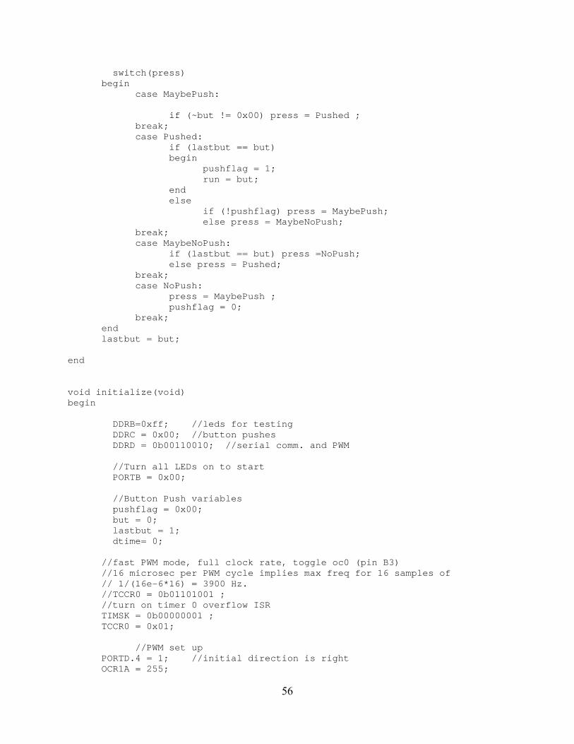
56

switch(press) begin case MaybePush: if (~but != 0x00) press = Pushed ; break; case Pushed: if (lastbut == but) begin pushflag = 1; run = but; end else if (!pushflag) press = MaybePush; else press = MaybeNoPush; break; case MaybeNoPush: if (lastbut == but) press =NoPush; else press = Pushed; break; case NoPush: press = MaybePush ; pushflag = 0; break; end lastbut = but; end void initialize(void) begin DDRB=0xff; //leds for testing DDRC = 0x00; //button pushes DDRD = 0b00110010; //serial comm. and PWM //Turn all LEDs on to start PORTB = 0x00; //Button Push variables pushflag = 0x00; but = 0; lastbut = 1; dtime= 0; //fast PWM mode, full clock rate, toggle oc0 (pin B3) //16 microsec per PWM cycle implies max freq for 16 samples of // 1/(16e-6*16) = 3900 Hz. //TCCR0 = 0b01101001 ; //turn on timer 0 overflow ISR TIMSK = 0b00000001 ; TCCR0 = 0x01; //PWM set up PORTD.4 = 1; //initial direction is right OCR1A = 255;

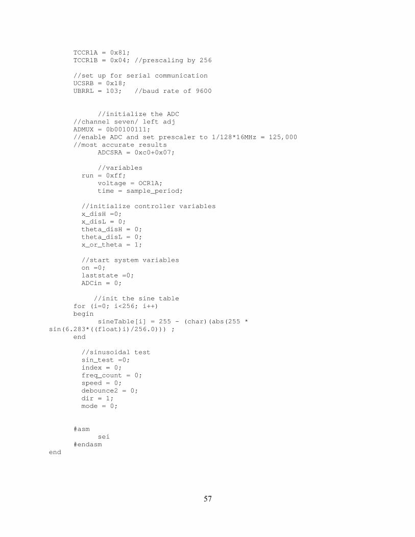
57

TCCR1A = 0x81; TCCR1B = 0x04; //prescaling by 256 //set up for serial communication UCSRB = 0x18; UBRRL = 103; //baud rate of 9600 //initialize the ADC //channel seven/ left adj ADMUX = 0b00100111; //enable ADC and set prescaler to 1/128*16MHz = 125,000 //most accurate results ADCSRA = 0xc0+0x07; //variables run = 0xff; voltage = OCR1A; time = sample_period; //initialize controller variables x_disH =0; x_disL = 0; theta_disH = 0; theta_disL = 0; x_or_theta = 1; //start system variables on =0; laststate =0; ADCin = 0; //init the sine table for (i=0; i<256; i++) begin sineTable[i] = 255 - (char)(abs(255 * sin(6.283*((float)i)/256.0))) ; end //sinusoidal test sin_test =0; index = 0; freq_count = 0; speed = 0; debounce2 = 0; dir = 1; mode = 0; #asm sei #endasm end

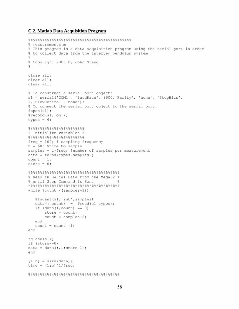
58

C.2. Matlab Data Acquisition Program %%%%%%%%%%%%%%%%%%%%%%%%%%%%%%%%%%%%%%%%%%%% % measurements.m % This program is a data acquisition program using the serial port in order % to collect data from the inverted pendulum system. % % Copyright 2005 by John Stang % close all; clear all; clear all; % To construct a serial port object: s1 = serial('COM1', 'BaudRate', 9600,'Parity', 'none', 'StopBits', 1,'FlowControl','none'); % To connect the serial port object to the serial port: fopen(s1); %record(s1,'on'); types = 6; %%%%%%%%%%%%%%%%%%%%%%%% % Initialize variables % %%%%%%%%%%%%%%%%%%%%%%%% freq = 100; % sampling frequency t = 60; %time to sample samples = t*freq; %number of samples per measurement data = zeros(types,samples); count = 1; store = 0; %%%%%%%%%%%%%%%%%%%%%%%%%%%%%%%%%%%%%%% % Read in Serial Data From the Mega32 % % until Stop Command is Sent % %%%%%%%%%%%%%%%%%%%%%%%%%%%%%%%%%%%%%%% while (count <(samples+1)) %fscanf(s1,'int',samples) data(:,count) = fread(s1,types); if (data(1,count) == 0) store = count; count = samples+2; end count = count +1; end fclose(s1); if (store~=0) data = data(:,1:store-1); end [a b] = size(data); time = (1:b)*1/freq; %%%%%%%%%%%%%%%%%%%%%%%%%%%%%%%%%%%%%%%

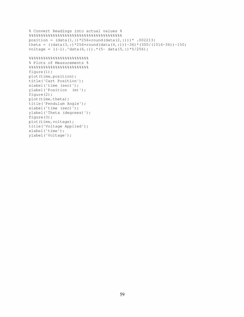
59

% Convert Readings into actual values % %%%%%%%%%%%%%%%%%%%%%%%%%%%%%%%%%%%%%%% position = (data(1,:)*256+round(data(2,:)))* .002213; theta = ((data(3,:)*256+round(data(4,:)))-36)*(300/(1016-36))-150; voltage = ((-1).^data(6,:)).*(5- data(5,:)*5/256); %%%%%%%%%%%%%%%%%%%%%%%%% % Plots of Measurements % %%%%%%%%%%%%%%%%%%%%%%%%% figure(1); plot(time,position); title('Cart Position'); xlabel('time (sec)'); ylabel('Position (m)'); figure(2); plot(time,theta); title('Pendulum Angle'); xlabel('time (sec)'); ylabel('Theta (degrees)'); figure(3); plot(time,voltage); title('Voltage Applied'); xlabel('time'); ylabel('Voltage');

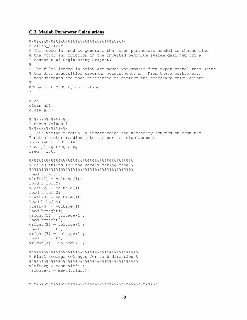
60

C.3. Matlab Parameter Calculations %%%%%%%%%%%%%%%%%%%%%%%%%%%%%%%%%%%%%%%% % alpha_calc.m % This code is used to generate the three parameters needed to charaterize % the motor and friction in the inverted pendulum system designed for a % Master's of Engineering Project. % % The files loaded in below are saved workspaces from experimental runs using % the data acquisition program, measurements.m. From these workspaces, % measurements are then referenced to perform the necessary calculations. % %Copyright 2005 by John Stang % clc; clear all; close all; %%%%%%%%%%%%%%%% % Known Values % %%%%%%%%%%%%%%%% % This variable actually incorporates the necessary conversion from the % poteniometer reading into the correct displacement sprocket = .0023316; % Sampling Frequency freq = 100; %%%%%%%%%%%%%%%%%%%%%%%%%%%%%%%%%%%%%%%%%%% % Calculations for the barely moving case % %%%%%%%%%%%%%%%%%%%%%%%%%%%%%%%%%%%%%%%%%%% load bmleft1; vleft(1) = voltage(1); load bmleft2; vleft(2) = voltage(1); load bmleft3; vleft(3) = voltage(1); load bmleft4; vleft(4) = voltage(1); load bmright1; vright(1) = voltage(1); load bmright2; vright(2) = voltage(1); load bmright3; vright(3) = voltage(1); load bmright4; vright(4) = voltage(1); %%%%%%%%%%%%%%%%%%%%%%%%%%%%%%%%%%%%%%%%%%%%% % Final average voltages for each direction % %%%%%%%%%%%%%%%%%%%%%%%%%%%%%%%%%%%%%%%%%%%%% vleftavg = mean(vleft); vrightavg = mean(vright); %%%%%%%%%%%%%%%%%%%%%%%%%%%%%%%%%%%%%%%%%%%%%%%%%%%%%

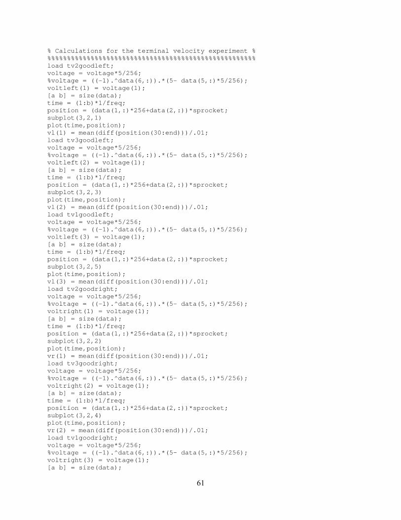
61

% Calculations for the terminal velocity experiment % %%%%%%%%%%%%%%%%%%%%%%%%%%%%%%%%%%%%%%%%%%%%%%%%%%%%% load tv2goodleft; voltage = voltage*5/256; %voltage = ((-1).^data(6,:)).*(5- data(5,:)*5/256); voltleft(1) = voltage(1); [a b] = size(data); time = (1:b)*1/freq; position = (data(1,:)*256+data(2,:))*sprocket; subplot(3,2,1) plot(time,position); vl(1) = mean(diff(position(30:end)))/.01; load tv3goodleft; voltage = voltage*5/256; %voltage = ((-1).^data(6,:)).*(5- data(5,:)*5/256); voltleft(2) = voltage(1); [a b] = size(data); time = (1:b)*1/freq; position = (data(1,:)*256+data(2,:))*sprocket; subplot(3,2,3) plot(time,position); vl(2) = mean(diff(position(30:end)))/.01; load tv1goodleft; voltage = voltage*5/256; %voltage = ((-1).^data(6,:)).*(5- data(5,:)*5/256); voltleft(3) = voltage(1); [a b] = size(data); time = (1:b)*1/freq; position = (data(1,:)*256+data(2,:))*sprocket; subplot(3,2,5) plot(time,position); vl(3) = mean(diff(position(30:end)))/.01; load tv2goodright; voltage = voltage*5/256; %voltage = ((-1).^data(6,:)).*(5- data(5,:)*5/256); voltright(1) = voltage(1); [a b] = size(data); time = (1:b)*1/freq; position = (data(1,:)*256+data(2,:))*sprocket; subplot(3,2,2) plot(time,position); vr(1) = mean(diff(position(30:end)))/.01; load tv3goodright; voltage = voltage*5/256; %voltage = ((-1).^data(6,:)).*(5- data(5,:)*5/256); voltright(2) = voltage(1); [a b] = size(data); time = (1:b)*1/freq; position = (data(1,:)*256+data(2,:))*sprocket; subplot(3,2,4) plot(time,position); vr(2) = mean(diff(position(30:end)))/.01; load tv1goodright; voltage = voltage*5/256; %voltage = ((-1).^data(6,:)).*(5- data(5,:)*5/256); voltright(3) = voltage(1); [a b] = size(data);

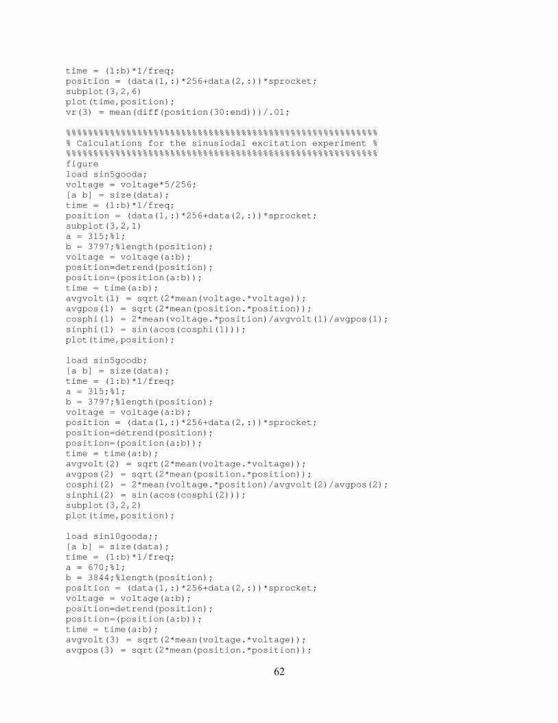
62

time = (1:b)*1/freq; position = (data(1,:)*256+data(2,:))*sprocket; subplot(3,2,6) plot(time,position); vr(3) = mean(diff(position(30:end)))/.01; %%%%%%%%%%%%%%%%%%%%%%%%%%%%%%%%%%%%%%%%%%%%%%%%%%%%%%%%% % Calculations for the sinusiodal excitation experiment % %%%%%%%%%%%%%%%%%%%%%%%%%%%%%%%%%%%%%%%%%%%%%%%%%%%%%%%%% figure load sin5gooda; voltage = voltage*5/256; [a b] = size(data); time = (1:b)*1/freq; position = (data(1,:)*256+data(2,:))*sprocket; subplot(3,2,1) a = 315;%1; b = 3797;%length(position); voltage = voltage(a:b); position=detrend(position); position=(position(a:b)); time = time(a:b); avgvolt(1) = sqrt(2*mean(voltage.*voltage)); avgpos(1) = sqrt(2*mean(position.*position)); cosphi(1) = 2*mean(voltage.*position)/avgvolt(1)/avgpos(1); sinphi(1) = sin(acos(cosphi(1))); plot(time,position); load sin5goodb; [a b] = size(data); time = (1:b)*1/freq; a = 315;%1; b = 3797;%length(position); voltage = voltage(a:b); position = (data(1,:)*256+data(2,:))*sprocket; position=detrend(position); position=(position(a:b)); time = time(a:b); avgvolt(2) = sqrt(2*mean(voltage.*voltage)); avgpos(2) = sqrt(2*mean(position.*position)); cosphi(2) = 2*mean(voltage.*position)/avgvolt(2)/avgpos(2); sinphi(2) = sin(acos(cosphi(2))); subplot(3,2,2) plot(time,position); load sin10gooda;; [a b] = size(data); time = (1:b)*1/freq; a = 670;%1; b = 3844;%length(position); position = (data(1,:)*256+data(2,:))*sprocket; voltage = voltage(a:b); position=detrend(position); position=(position(a:b)); time = time(a:b); avgvolt(3) = sqrt(2*mean(voltage.*voltage)); avgpos(3) = sqrt(2*mean(position.*position));

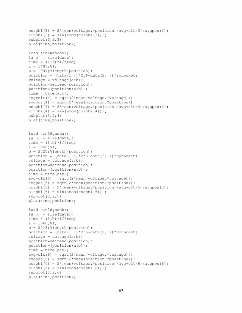
63

cosphi(3) = 2*mean(voltage.*position)/avgvolt(3)/avgpos(3); sinphi(3) = sin(acos(cosphi(3))); subplot(3,2,3) plot(time,position); load sin10goodb;; [a b] = size(data); time = (1:b)*1/freq; a = 1485;%1; b = 1997;%length(position); position = (data(1,:)*256+data(2,:))*sprocket; voltage = voltage(a:b); position=detrend(position); position=(position(a:b)); time = time(a:b); avgvolt(4) = sqrt(2*mean(voltage.*voltage)); avgpos(4) = sqrt(2*mean(position.*position)); cosphi(4) = 2*mean(voltage.*position)/avgvolt(4)/avgpos(4); sinphi(4) = sin(acos(cosphi(4))); subplot(3,2,4) plot(time,position); load sin20gooda;; [a b] = size(data); time = (1:b)*1/freq; a = 1650;%1; b = 2520;%length(position); position = (data(1,:)*256+data(2,:))*sprocket; voltage = voltage(a:b); position=detrend(position); position=(position(a:b)); time = time(a:b); avgvolt(5) = sqrt(2*mean(voltage.*voltage)); avgpos(5) = sqrt(2*mean(position.*position)); cosphi(5) = 2*mean(voltage.*position)/avgvolt(5)/avgpos(5); sinphi(5) = sin(acos(cosphi(5))); subplot(3,2,5) plot(time,position); load sin20goodb;; [a b] = size(data); time = (1:b)*1/freq; a = 1660;%1; b = 2018;%length(position); position = (data(1,:)*256+data(2,:))*sprocket; voltage = voltage(a:b); position=detrend(position); position=(position(a:b)); time = time(a:b); avgvolt(6) = sqrt(2*mean(voltage.*voltage)); avgpos(6) = sqrt(2*mean(position.*position)); cosphi(6) = 2*mean(voltage.*position)/avgvolt(6)/avgpos(6); sinphi(6) = sin(acos(cosphi(6))); subplot(3,2,6) plot(time,position);

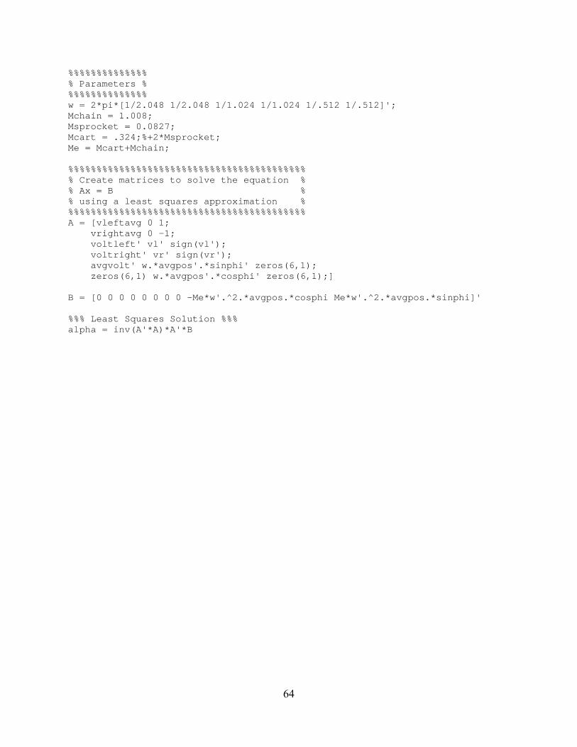
64

%%%%%%%%%%%%%% % Parameters % %%%%%%%%%%%%%% w = 2*pi*[1/2.048 1/2.048 1/1.024 1/1.024 1/.512 1/.512]'; Mchain = 1.008; Msprocket = 0.0827; Mcart = .324;%+2*Msprocket; Me = Mcart+Mchain; %%%%%%%%%%%%%%%%%%%%%%%%%%%%%%%%%%%%%%%%%% % Create matrices to solve the equation % % Ax = B % % using a least squares approximation % %%%%%%%%%%%%%%%%%%%%%%%%%%%%%%%%%%%%%%%%%% A = [vleftavg 0 1; vrightavg 0 -1; voltleft' vl' sign(vl'); voltright' vr' sign(vr'); avgvolt' w.*avgpos'.*sinphi' zeros(6,1); zeros(6,1) w.*avgpos'.*cosphi' zeros(6,1);] B = [0 0 0 0 0 0 0 0 -Me*w'.^2.*avgpos.*cosphi Me*w'.^2.*avgpos.*sinphi]' %%% Least Squares Solution %%% alpha = inv(A'*A)*A'*B

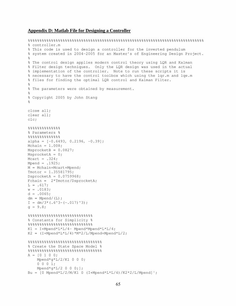
65

Appendix D: Matlab File for Designing a Controller %%%%%%%%%%%%%%%%%%%%%%%%%%%%%%%%%%%%%%%%%%%%%%%%%%%%%%%%%%%%%%%%%%%%%%%%%%%% % controller.m % This code is used to design a controller for the inverted pendulum % system created in 2004-2005 for an Master’s of Engineering Design Project. % % The control design applies modern control theory using LQR and Kalman % Filter design techniques. Only the LQR design was used in the actual % implementation of the controller. Note to run these scripts it is % necessary to have the control toolbox which using the lqr.m and lqe.m % files for finding the optimal LQR control and Kalman Filter. % % The parameters were obtained by measurement. % % Copyright 2005 by John Stang % close all; clear all; clc; %%%%%%%%%%%%%% % Parameters % %%%%%%%%%%%%%% alpha = [-0.6493, 0.2196, -0.39]; Mchain = 1.008; MsprocketB = 0.0827; MsprocketA = 0; Mcart = .324; Mpend = .1925; M = Mchain+Mcart+Mpend; Tmotor = 1.35581795; DsprocketA = 0.0759968; Fchain = 2*Tmotor/DsprocketA; L = .617; w = .0183; d = .0065; dm = Mpend/(L); I = dm/3*(.6^3-(-.017)^3); g = 9.8; %%%%%%%%%%%%%%%%%%%%%%%%%%%% % Constants for Simplicity % %%%%%%%%%%%%%%%%%%%%%%%%%%%% K1 = I+Mpend*L*L/4- Mpend*Mpend*L*L/4; K2 = (I+Mpend*L*L/4)*M*2/L/Mpend+Mpend*L/2; %%%%%%%%%%%%%%%%%%%%%%%%%%%%%%%% % Create the State Space Model % %%%%%%%%%%%%%%%%%%%%%%%%%%%%%%%% A = [0 1 0 0; Mpend*g*L/2/K1 0 0 0; 0 0 0 1; Mpend*g*L/2 0 0 0;]; Bu = [0 Mpend*L/2/M/K1 0 (I+Mpend*L*L/4)/K2*2/L/Mpend]';

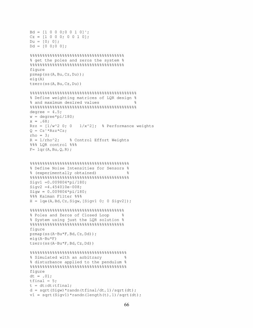
66

Bd = [1 0 0 0;0 0 1 0]'; Cz = [1 0 0 0; 0 0 1 0]; Du = [0; 0]; Dd = [0 0;0 0]; %%%%%%%%%%%%%%%%%%%%%%%%%%%%%%%%%%%%%% % get the poles and zeros the system % %%%%%%%%%%%%%%%%%%%%%%%%%%%%%%%%%%%%%% figure pzmap(ss(A,Bu,Cz,Du)); eig(A) tzero(ss(A,Bu,Cz,Du)) %%%%%%%%%%%%%%%%%%%%%%%%%%%%%%%%%%%%%%%%%%% % Define weighting matrices of LQR design % % and maximum desired values % %%%%%%%%%%%%%%%%%%%%%%%%%%%%%%%%%%%%%%%%%%% degree = 4.5; w = degree*pi/180; x = .68; Rzz = [1/w^2 0; 0 1/x^2]; % Performance weights Q = Cz'*Rzz*Cz; rho = 3; R = 1/rho^2; % Control Effort Weights %%% LQR control %%% F= lqr(A,Bu,Q,R); %%%%%%%%%%%%%%%%%%%%%%%%%%%%%%%%%%%%%%%% % Define Noise Intensities for Sensors % % (experimentally obtained) % %%%%%%%%%%%%%%%%%%%%%%%%%%%%%%%%%%%%%%%% Sigv1 =0.009804*pi/180; Sigv2 =4.454010e-008; Sigw = 0.009804*pi/180; %%% Kalman Filter %%% H = lqe(A,Bd,Cz,Sigw,[Sigv1 0; 0 Sigv2]); %%%%%%%%%%%%%%%%%%%%%%%%%%%%%%%%%%%%%% % Poles and Zeros of Closed Loop % % System using just the LQR solution % %%%%%%%%%%%%%%%%%%%%%%%%%%%%%%%%%%%%%% figure pzmap(ss(A-Bu*F,Bd,Cz,Dd)); eig(A-Bu*F) tzero(ss(A-Bu*F,Bd,Cz,Dd)) %%%%%%%%%%%%%%%%%%%%%%%%%%%%%%%%%%%%%%% % Simulated with an arbitrary % % disturbance applied to the pendulum % %%%%%%%%%%%%%%%%%%%%%%%%%%%%%%%%%%%%%%% figure dt = .01; tfinal = 5; t = dt:dt:tfinal; d = sqrt(Sigw)*randn(tfinal/dt,1)/sqrt(dt); v1 = sqrt(Sigv1)*randn(length(t),1)/sqrt(dt);

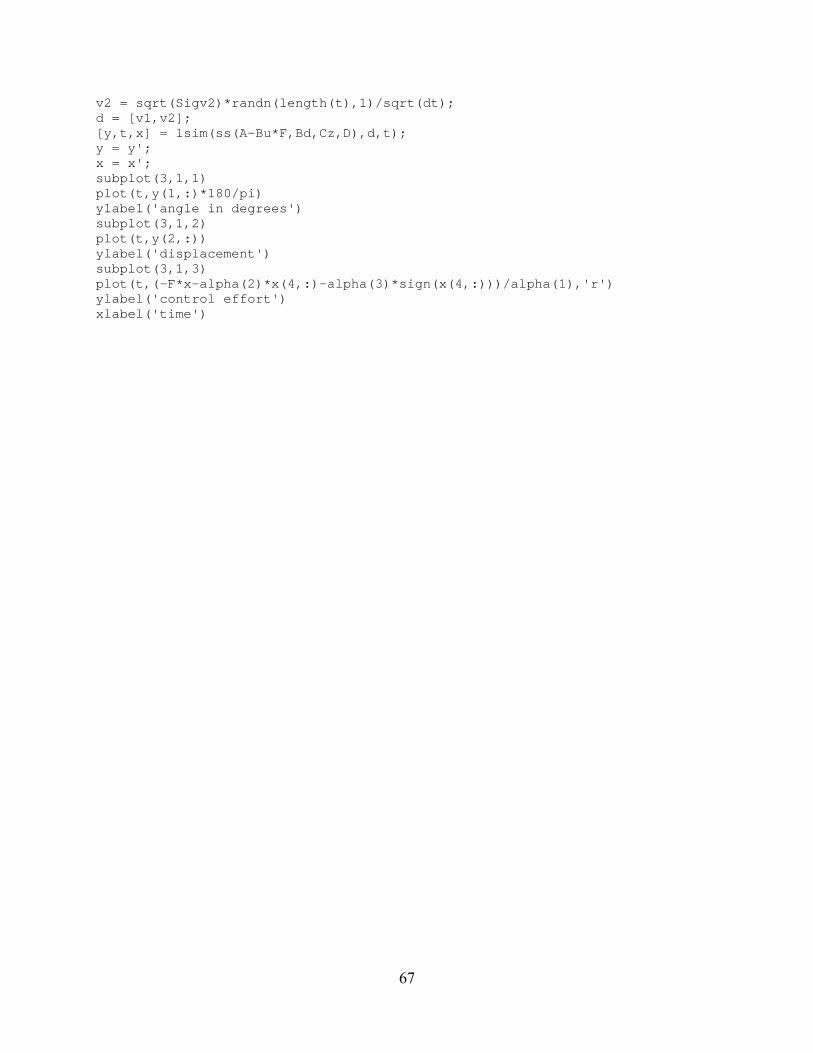
67

v2 = sqrt(Sigv2)*randn(length(t),1)/sqrt(dt); d = [v1,v2]; [y,t,x] = lsim(ss(A-Bu*F,Bd,Cz,D),d,t); y = y'; x = x'; subplot(3,1,1) plot(t,y(1,:)*180/pi) ylabel('angle in degrees') subplot(3,1,2) plot(t,y(2,:)) ylabel('displacement') subplot(3,1,3) plot(t,(-F*x-alpha(2)*x(4,:)-alpha(3)*sign(x(4,:)))/alpha(1),'r') ylabel('control effort') xlabel('time')

68

Appendix E: C Source File for the Controller //CopyRight 2005 by John Stang //controller.c #include <Mega32.h> #include <stdio.h> #include <stdlib.h> #include <delay.h> #include <math.h> // for sine #define begin { #define end } #define countMS 62 //ticks/mSec #define sample_period 10 void initialize(void); void sample(void); unsigned char count; //millisecond counter unsigned char time; //counter for sampling unsigned char but; //debouncing button variblaes //ADC conversion variables unsigned char x_or_theta; //sampled outputs unsigned char x_disH; unsigned char x_disL; unsigned char theta_disH; unsigned char theta_disL; unsigned char voltage; unsigned char dir; unsigned int ADCin; signed int theta_dis; signed int x_dis; //controller variables signed int x_ref; signed int theta_ref; float x; float last_x; float x_dot; float theta; float last_theta; float theta_dot; float u,temp2; unsigned int temp; //Controller Values for a working controller float f[4] = {74.0346, 16.2864, 4.4118, 7.7452}; //Motor and Friction Parameters float alpha[3] = {-0.6493, 0.2196, -0.385}; //running system variables unsigned char on; unsigned char laststate;

69

//Interrupt used to set up time base interrupt [TIM0_OVF] void sgen(void) begin //generate rising amplitude // 62 counts is about 1 mSec count--; if (0 == count ) begin count=countMS; time++; end//end millisecond timer end //end interrupt void main(void) begin initialize(); while(1) begin //SAMPLE AND OUTPUT TO MATLAB if (time >= sample_period) sample(); /*Check the ADC for a measurement. This will alternate between the angle measurement and displacement measurement. These are free-running so both values will be as accurate as possible when samples need to be used for controlling the pendulum.*/ if (ADCSRA.4==1) begin ADCin = ADCW>>6; if (x_or_theta==1) begin x_disH = (char)(ADCin>>8); x_disL = (char)(ADCin); x_dis = ADCin; ADMUX.0 = 1; //switch to theta x_or_theta = 0; end else begin theta_disH = (char)(ADCin>>8); theta_disL = (char)(ADCin); theta_dis = ADCin; ADMUX.0 = 0; //switch to x x_or_theta = 1; end //start another conversion ADCSRA = ADCSRA | 0x50; end //Determine Button Presses to turn the control on or off but = PINC; switch (~but) begin

70

case (0x01): on = 1; break; case (0x02): on = 0; putchar(0); putchar(0); putchar(0); putchar(0); putchar(0); putchar(0); break; end//end switch end //end while end //end main /*This function using the most recent samples from the ADC to determine the control effort require to keep the pendulum balanced as well as output the corresponding data to Matlab */ //!!!!!!!!!!!!!! IMPLEMENT CONTROLLER IN HERE !!!!!!!!!!!!!! void sample(void) begin time = 0; //Initialize References for start if (~laststate & on) begin x_ref = (x_dis); theta_ref = (theta_dis); end laststate = on; //Displacement, Angle, and voltage conversions //!!!!!CONTROLLER IS ALSO IMPLEMENTED WITHIN THIS IF STATEMENT !!!! if (on) begin last_x = x; x = ((float)(x_dis-x_ref)*.0023316); last_theta = theta; theta = ((float)(theta_dis - theta_ref))* 0.0051138;//0.2930*PI/180);//*0.3061;//assumes 300 degrees voltage = (((float)((-1)^dir))*(1-((float)(OCR1A))/255)*5); //max voltage might be less than 20, may need to adjust x_dot = (((float)(x-last_x))*sample_period/1000); theta_dot = (((float)(theta-last_theta))*sample_period/1000); /* !!!!!!!INSERT CONTROLLER HERE !!!!!!!!!!!!!! in the form f[0] = value0; f[1] = value1;

71

f[2] = value2; f[3] = value3; */ //calculates generic force u = -(f[0]*theta+f[1]*theta_dot+f[2]*x+f[3]*x_dot); //converts generic control into a voltage using the nonlinear //relationship and also scales to use full PWM range temp2 = ((u-alpha[1]*x_dot-alpha[2]*fsign(x_dot))/alpha[0])*50; //determines the direction of the control if (fsign(temp2)==1) dir = 0; else dir = 1; PORTD.4 = dir; PORTB = ~dir; //sets PWM to magnitude of control effort temp = ((int)(abs(temp2))); // 255/5 if (temp > 255) OCR1A = 0; else OCR1A = 255-temp; putchar(x_disH); putchar(x_disL); //raw angle data putchar(theta_disH); putchar(theta_disL); //raw voltage data putchar((char)(OCR1A)); putchar(dir); end else OCR1A=255; end //end sample void initialize(void) begin DDRB=0xff; //leds for testing DDRC = 0x00; //button pushes DDRD = 0b00110010; //serial comm. and PWM //Turn all LEDs on to start PORTB = 0xff; //fast PWM mode, full clock rate, toggle oc0 (pin B3) //16 microsec per PWM cycle implies max freq for 16 samples of // 1/(16e-6*16) = 3900 Hz. //TCCR0 = 0b01101001 ; //turn on timer 0 overflow ISR

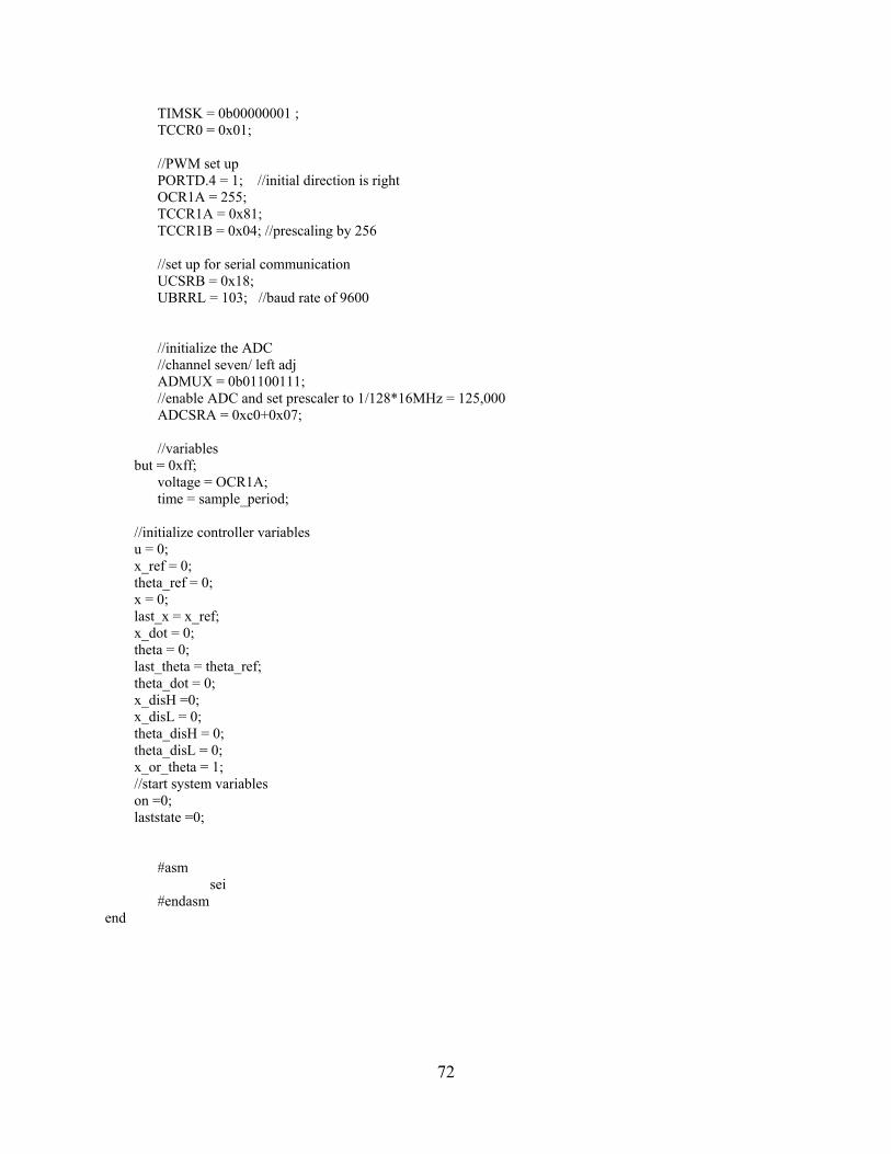
72

TIMSK = 0b00000001 ; TCCR0 = 0x01; //PWM set up PORTD.4 = 1; //initial direction is right OCR1A = 255; TCCR1A = 0x81; TCCR1B = 0x04; //prescaling by 256 //set up for serial communication UCSRB = 0x18; UBRRL = 103; //baud rate of 9600 //initialize the ADC //channel seven/ left adj ADMUX = 0b01100111; //enable ADC and set prescaler to 1/128*16MHz = 125,000 ADCSRA = 0xc0+0x07; //variables but = 0xff; voltage = OCR1A; time = sample_period; //initialize controller variables u = 0; x_ref = 0; theta_ref = 0; x = 0; last_x = x_ref; x_dot = 0; theta = 0; last_theta = theta_ref; theta_dot = 0; x_disH =0; x_disL = 0; theta_disH = 0; theta_disL = 0; x_or_theta = 1; //start system variables on =0; laststate =0; #asm sei #endasm end

73

Appendix F: Parts List and Cost

Part Actual Cost Cost for this Project Atmel Mega32 $8.28 Free (Supplied by Dr. Land) STK500 $79.99 On loan from Dr. Land LMD18200 $11.69 sampled 4N35 $0.37 Free (Laboratory supplies) Max233 $8.93 Free (Supplied by Dr. Land) PCB Board $5.00 Free (Supplied by Dr. Land) LM34 $0.34 Free (Supplied by Dr. Land) Power Supply (20V) N/A On Loan from ECE Dept. Serial Cables and Power Supplies for STK500 and Protoboard

N/A On Loan from Dr. Land

Resistors, Capacitors, Diodes, and other basic components

N/A Free (Laboratory supplies)

Motor (Surplus Center) $19.99 $39.98 (needed 2 because 1st broke)

Drive Sprocket $18.63 $18.63 Free Spinning Sprocket $7.69 $7.69 Chain $10.00 $10.00 Track $40.00 Free (Supplied by Dr. Land) Switches N/A Free (Supplied by Dr. Land) Pendulum Free Scrap Metal in Machine Shop Wood, Wheels, Screws, Etc ~$25.00 ~$25.00 Matchbox Cars $1.98 $1.98 Total Cost $237.89 $103.28

*Note that the actually cost could be reduced significantly if the STK500 programming board isn’t used. This part isn’t necessary, but does make programming the Mega32 easier.

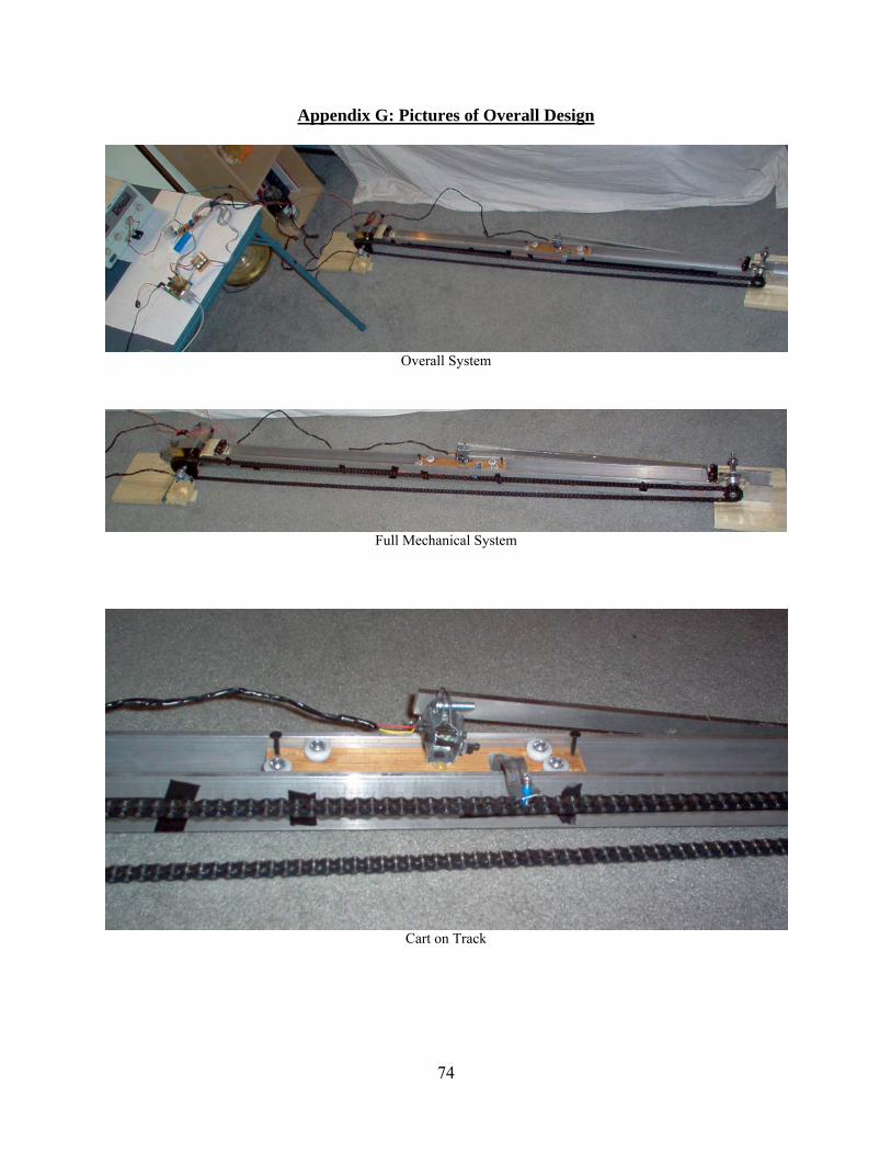
74

Appendix G: Pictures of Overall Design

Overall System

Full Mechanical System

Cart on Track

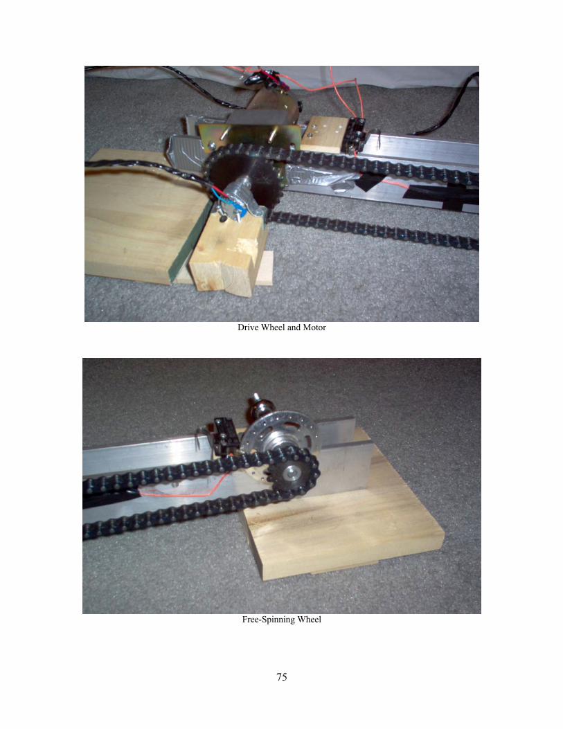
75

Drive Wheel and Motor

Free-Spinning Wheel

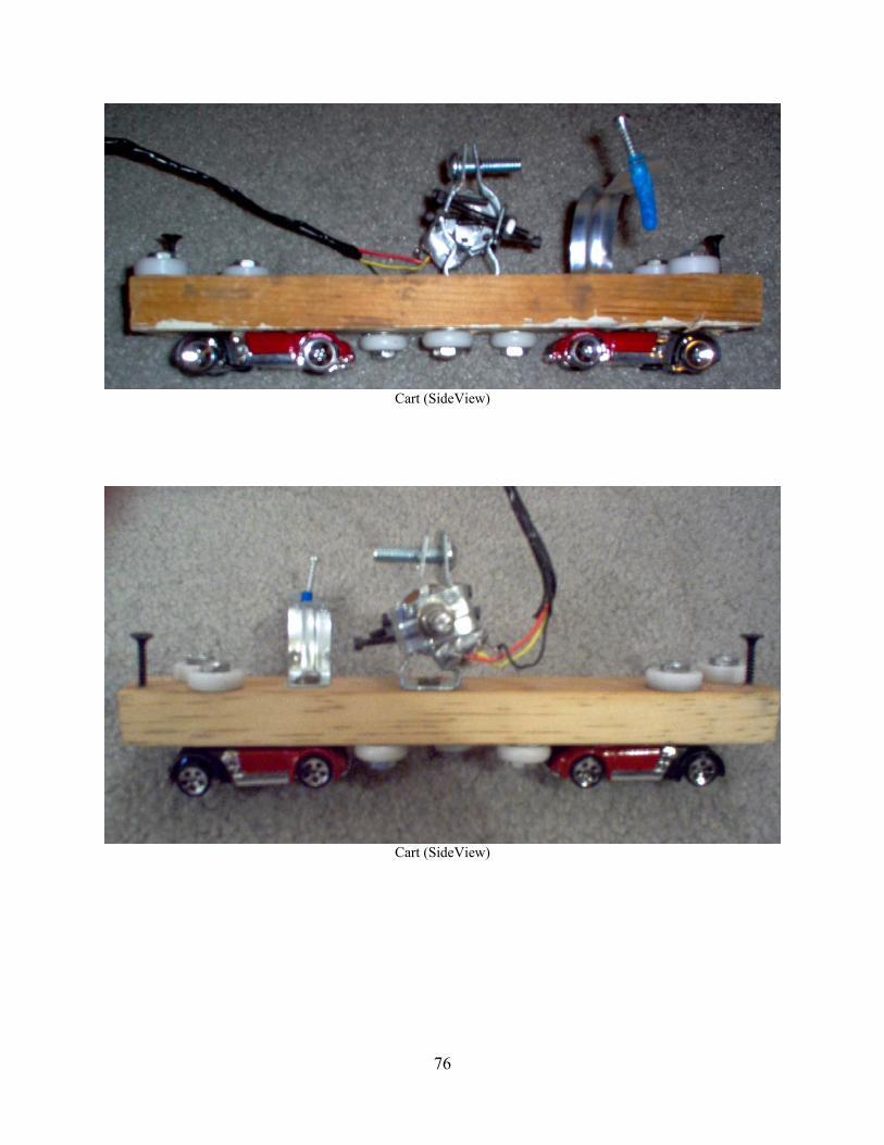
76

Cart (SideView)

Cart (SideView)

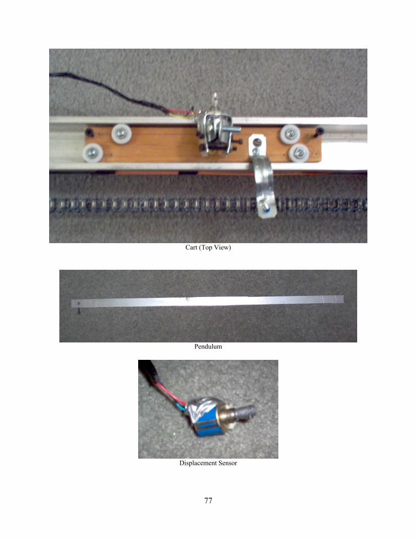
77

Cart (Top View)

Pendulum

Displacement Sensor

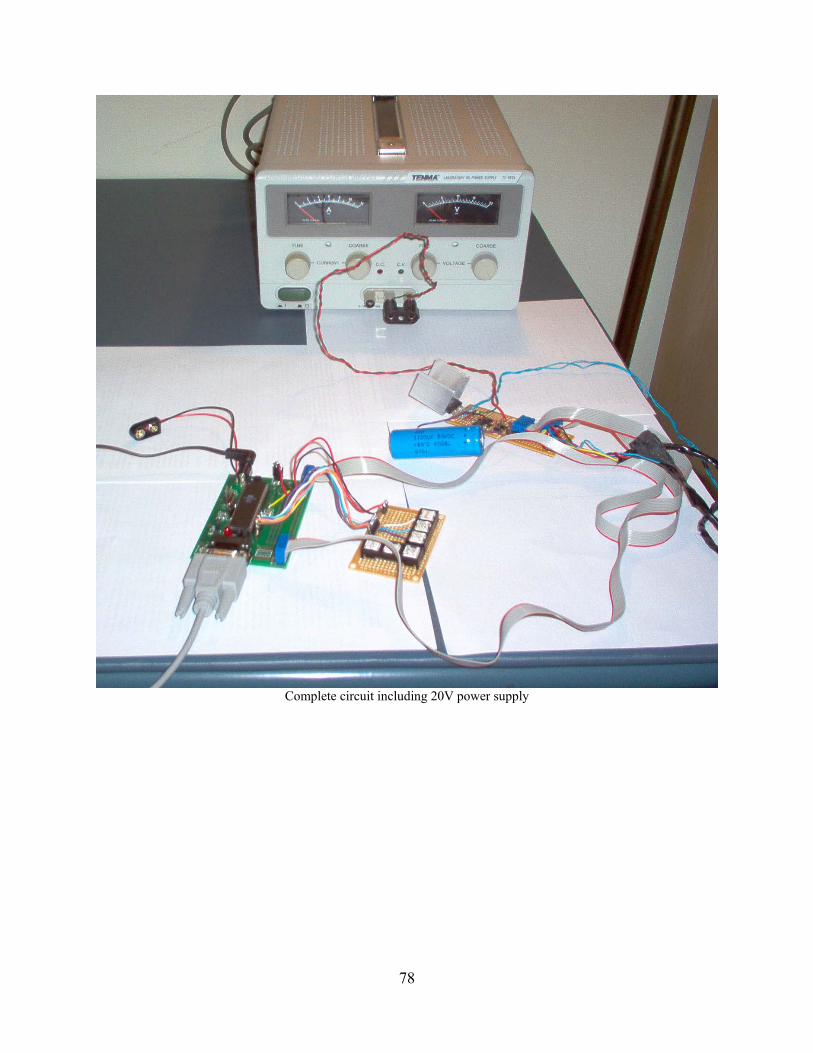
78

Complete circuit including 20V power supply

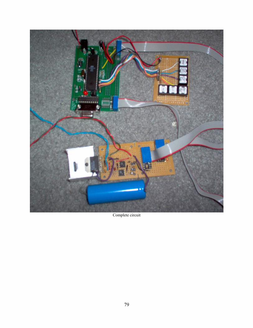
79

Complete circuit

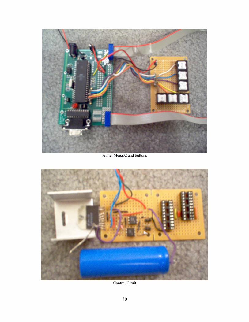
80

Atmel Mega32 and buttons

Control Ciruit