THE SPLIT BREGMAN METHOD FOR L1 REGULARIZEDPROBLEMS

TOM GOLDSTEIN, STANLEY OSHER

Abstract. The class of l1-regularized optimization problems has received much attention re-cently because of the introduction of “compressed sensing,” which allows images and signals to bereconstructed from small amounts of data. Despite this recent attention, many l1-regularized prob-lems still remain difficult to solve, or require techniques that are very problem-specific. In this paper,we show that Bregman iteration can be used to solve a wide variety of constrained optimization prob-lems. Using this technique, we propose a “Split Bregman” method, which can solve a very broadclass of l1-regularized problems. We apply this technique to the ROF functional for image denoising,and to a compressed sensing problem that arises in Magnetic Resonance Imaging.

Key words. Constrained Optimization, l1 regularization, compressed sensing, total variationdenoising.

1. Introduction. The category of l1-regularized problems includes many im-portant problems in engineering, computer, and imaging science. The general formfor such problems is

minu|Φ(u)|+H(u)(1.1)

where | · | denotes the l1-norm, and both |Φ(u)| and H(u) are convex functions. Manyimportant problems in imaging science (and other computational areas) can be posedas l1-regularized optimization problems. Some common examples of this include thefollowing:

“TV/ROF Denoising: ” minu‖u‖BV +

µ

2‖u− f‖22(1.2)

“Basis Pursuit/Compressed Sensing: ” minuJ(u) +

µ

2‖Au− f‖22(1.3)

where J(u) is some regularizing functional, usually in the form of a BV or Besovnorm.

The Rudin-Osher-Fatemi (ROF) functional (1.2), despite its simple form, hasproved to be very difficult to minimize by conventional methods. Total variation basedimage restoration was first introduced in [22]. In that paper, the authors propose tominimize this energy using a gradient projection method. While this approach issimple, the non-linearity and poor conditioning of the problem make this approachvery slow. Several authors have proposed improved time-stepping schemes that resultin better performance, such as those presented in [26, 15]. A more efficient class ofsolvers are those based on Newton’s method. One such algorithm was presented in [9],in which the preconditioned conjugate gradient method is used to invert the Hessianat each step. A somewhat more efficient implementation of a second-order methodwas proposed by Vogel et. al. in [25], where an algebraic multigrid preconditioner isused to accelerate the method.

Still, the most efficient solver for the ROF problem was proposed by Darbonand Sigelle in [10]. In this work, the ROF functional was approximated using ananisotropic BV norm. It was shown that, using this formulation, the resulting problemcould be solved very quickly using graph cuts [3].

1

Problems of the form (1.3) have received a lot of attention recently because of theintroduction of compressed sensing techniques, which allow high resolution images andsignals to be reconstructed from a small amount of data [7, 6, 11]. This formulationhas been shown to be useful in many areas, including medical imaging [16, 17], radar[1], and other signal processing applications. Compressed sensing is based on theidea that a signal can be reconstructed from a very small number of measurements,provided that these measurements are obtained in the correct basis. The particularapplication of compressed sensing which we will focus on is MR image reconstruction,or “Sparse MRI” [16, 14]. The goal of sparse MRI is to solve

minuJ(u) such that ‖Fu− f‖2 = 0.

Here, f represents the so-called “compressed sensing data,” which consists of samplesof the Fourier transform of the unknown image. F comprises a subset of the rows ofa Fourier matrix, u represents the unknown image that we wish to reconstruct, andJ(·) is a properly chosen l1-regularization term. The unconstrained formulation forthis problem was introduced in [14], where a Bregman iterative approach [4] was usedto obtain solutions to “denoising” problems of the form

minuJ(u) such that ‖Fu− f‖2 < σ.(1.4)

Because of the presence of an l1-regularization term, optimization problems of theform (1.4) are still very difficult to solve. Several authors have applied classical opti-mization schemes, such as interior point methods, to problems of these forms. In [23],CS problems were reformulated as quadratic programming problems which were thensolved using the code “l1 ls,” which is claimed to be one of the most efficient solversfor general compressed sensing problems. Another notable interior-point approach isthe code “l1-magic,” which formulates a CS problem as a second order cone program,and enforces inequality constraints using a logarithmic barrier potential [7].

In the special case where the CS problem can be written in the form

minu|u| such that ‖Au− f‖2 < σ(1.5)

a relatively new class of methods can be used that reduce the CS problem to setof simpler problems using linearization. The first of these methods is the “FixedPoint Continuation” method (FPC) introduced in [13] by Hale, Yin, and Zhang. Thismethod solves the unconstrained problem

minu|u|+ µ

2‖Au− f‖22(1.6)

by iteratively performing gradient descent steps.By applying the Bregman iteration scheme in [21, 14], it is also possible to solve

the constrained problem (1.5) using FPC/Bregman. This is done by iteratively solvingthe unconstrained problem (1.6), and then modifying the value of f used in the nextiteration.

Rather than solving the unconstrained problem and then performing a Bregmanupdate separately, these two steps were elegantly combined in the Linearized BregmanAlgorithm [30]. Linearized Bregman solves the problem (1.5) by iteratively solving

vk+1 = vk +AT (f −Auk)uk+1 = δ ∗ shrink(vk+1, 1/µ)

2

for k = 1, 2, · · ·n. The algorithm is terminated when the denoising constraint in (1.5)is met. It was shown in [5, 20] that un will be a suitable approximation to the solutionof (1.5) provided that appropriate values are chosen for the parameters µ and δ.

While the FPC and Linearized Bregman algorithms are extremely efficient, theycan only solve problems which can be put into the form (1.6). Because the gradientoperator is not invertible, these algorithms cannot be used to solve problems involvingthe BV norm. Also, these schemes cannot solve optimization problems involvingmultiple l1-regularization terms. For these reasons, it is difficult to apply the FPCand linearized Bregman methods to image processing problems. For example, it hasbeen noted by many authors [16, 24] that optimal MRI reconstruction is obtainedusing a combination of both the BV norm and Besov norm, B1,1. In this case, thisproblem can be written

minu‖u‖BV + ‖u‖H +

µ

2‖Fu− f‖22

where ‖ · ‖BV = ‖∇u‖1 is the “bounded variation” norm, and ‖u‖H = ‖Hu‖1 denotesthe “Besov” norm with respect to the Haar wavelet transform. We will later addressthis particular form of the compressed sensing problem.

In this paper, we will present a general technique that can be used to solve mostcommon l1-regularized problems efficiently. Furthermore, the optimization schemewe employ can be generalized to solve a very broad range of equality-constrainedoptimization problems, some of which may be difficult to solve by existing techniques.

The contents of this paper are organized as follows: We begin with a brief dis-cussion of constrained optimization problems and classical penalty function methods.We then review the concept of Bregman iteration, and use it to derive a general prin-ciple for solving constrained optimization problems. We will then define the “SplitBregman” method, and show how it can be used to solve the general l1-regularizedoptimization problem (1.1). Finally, we will apply the Split Bregman technique to TVdenoising and compressed sensing problems to demonstrate its efficiency. The lattermay involve BV, Besov, or multiple regularizers.

1.1. Constrained Optimization Problems. Consider a convex energy func-tional, E, and some linear function, A : Rn → Rm. We wish to solve the generalizedconstrained optimization problem

minuE(u) s.t. Au = b.(1.7)

This problem can be very difficult to solve directly if E is non-differentiable.In order to make (1.7) simpler to solve, we wish to convert it into an unconstrained

optimization problem. One common method for doing this it to use a penalty func-tion/continuation method, which approximates (1.7) by a problem of the form

minuE(u) +

λk2‖Au− b‖22.(1.8)

where λ1 < λ2 < · · · < λN is an increasing sequence of penalty function weights[2, 19]. In order to enforce that H(u) ≈ 0, we must choose λN to be extremely large.

Unfortunately, for many problems, choosing a large value for λ makes (1.8) ex-tremely difficult to solve numerically. We often wish to solve (1.8) by a Newton-typemethod, which requires us to invert the Hessian of the objective function. However,as λk → ∞, the condition number of the Hessian approaches infinity, making it im-practical to use fast iterative methods (such as Conjugate Gradient or Gauss-Seidel

3

methods)[2, 19]. Also, for many applications, λk must be increased in very smallsteps, making the method less efficient.

In the next section, we will show that Bregman iteration can be used to reduce(1.7) to a short sequence of unconstrained problems. In this sense, Bregman iterationis an alternative to conventional penalty function methods.

2. Bregman Iteration. Bregman iteration is a concept that originated in func-tional analysis for finding extrema of convex functionals [4]. Bregman iteration wasfirst used in image processing by Osher at. al. in [21], where it was applied to theROF model for TV denoising. Bregman iteration has also been applied to solve thebasis pursuit problem in [30, 5, 20], and was subsequently applied to medical imagingproblems in [14]. Rather than focus on specific applications, we will present here ageneral formulation of this technique.

We begin with the concept of “Bregman Distance.” The Bregman Distance asso-ciated with a convex function E at the point v is

DpE(u, v) = E(u)− E(v)− 〈p, u− v〉

where p is in the subgradient of E at v. Clearly, this is not a distance in the usualsense because it is not in general symmetric. However, it does measure closeness inthe sense that Dp

E(u, v) ≥ 0, and DpE(u, v) ≥ Dp

E(w, v) for w on the line segmentbetween u and v.

Again, consider two convex energy functionals, E and H, defined over Rn withminu∈Rn H(u) = 0. The associated unconstrained minimization problem is

minuE(u) + λH(u).(2.1)

We can modify this problem by iteratively solving

uk+1 = minuDpE(u, uk) + λH(u)(2.2)

= minuE(u)− 〈pk, u− uk〉+ λH(u)(2.3)

as was suggested by Bregman in [4].For simplicity, we will assume that H is differentiable. In this case, we have

that 0 ∈ ∂(DpE(u, uk) +λH(u)) where this sub-differential is evaluated at uk+1. Since

pk+1 ∈ ∂E(uk+1) at this location, we have that

pk+1 = pk −∇H(uk+1).

In [21], the authors analyze the convergence of Bregman iterative schemes. Inparticular, it is shown that, under fairly weak assumptions on E and H, that H(uk)→0 as k →∞.

Two particular convergence results from [21] are especially relevant here, and sowe restate them.

Theorem 2.1. Assume that E and H are convex functionals, and that H is dif-ferentiable. We also assume that solutions to the sub-problems in (2.2) exist. Wethen have

1) Monotonic decrease in H: H(uk+1) ≤ H(uk)2) Convergence to a minimizer of H : H(uk) ≤ H(u∗) + J(u∗)/k

In addition to these convergence results, Bregman iteration has several nice de-noising properties which are discussed and proved in [21] and [14].

4

2.1. Constrained Optimization via Bregman Iteration. In this section,we present a method for solving a wide variety of constrained optimization problemswithout using continuation. We first show that Bregman iteration can be used tosolve the constrained problem (1.7). We will then discuss a simplified form of Bregmaniteration, which is equivalent to “adding the noise back” as is done with ROF denoising[21]. Finally, we will discuss the convergence properties of this method.

We wish to solve

minuE(u) such that Au = b(2.4)

for some linear operator A and vector b. To apply formula (2.1), we make this intoan unconstrained problem using a quadratic penalty function:

minuE(u) +

λ

2‖Au− b‖22(2.5)

For small λ, the penalty function does not accurately enforce the constraint. Theconventional solution to this problem is to let λ→∞. Rather, we apply the Bregmaniteration (2.2), and iteratively minimize:

uk+1 = minuDpE(u, uk) +

λ

2‖Au− b‖22(2.6)

= minuE(u)− 〈pk, u− uk〉+

λ

2‖Au− b‖22(2.7)

pk+1 = pk − λAT (Auk+1 − b)(2.8)

Bregman iterations of this form were considered in [30] and [21]. Here, it isshown that, when A is linear, this seemingly complicated iteration is equivalent tothe simplified method:

uk+1 = minuE(u) +

λ

2‖Au− bk‖22(2.9)

bk+1 = bk + b−Auk(2.10)

In other words, we simply add the error in the constraint back to the right hand side.This is the analog of “adding back the noise” in the ROF model for TV denoising[21].

Because of the equivalence of (2.6-2.8) and (2.9-2.10), and the convergence resultsof theorem 2.1, we have that

limk→∞

Auk = b(2.11)

where convergence is in the 2-norm sense. In other words, for large k, the iterates uk

satisfy the constraint condition to an arbitrarily high degree of accuracy.We now need to show that a solution, u∗, of Au = b obtained through (2.9-2.10)

is indeed a solution to the original constrained problem (2.4). Note that Bregmaniteration was used to solve a constrained optimization problem in [30]. In this paper,the authors assume a specific form for the operator A. Here, we broaden this resultand present a very simple proof.

5

Theorem 2.2. Let H : Rn → R be convex. Let A : Rn → Rm be linear. Considerthe algorithm (2.9-2.10). Suppose that some iterate, u∗, satisfies Au∗ = b. Then u∗

is a solution to the original constrained problem (2.4).Proof: Let u∗ and b∗ be such that Au∗ = b, and

u∗ = minuE(u) +

λ

2‖Au− b∗‖22(2.12)

Let u be a true solution to (2.4). Then Au∗ = b = Au, which implies that

‖Au∗ − b∗‖22 = ‖Au− b∗‖22(2.13)

Because u∗ satisfies (2.12), we have

E(u∗) +λ

2‖Au∗ − b∗‖22 ≤ E(u) +

λ

2‖Au− b∗‖22.(2.14)

Finally, note that (2.13) and (2.14) together imply

E(u∗) ≤ E(u).

Because u satisfies the original optimization problem, this inequality can be sharpenedto an equality, showing that u∗ solves (2.4).

This shows that, provided (2.9-2.10) converges in the sense of (2.11), the iteratesuk will get arbitrarily close to a solution of the original constrained problem (1.7).Note the generality of the above theorem. The proof does not explicitly use thelinearity of A, and in fact this condition is not required for the theorem to hold. Theapplication of this method to problems in which A is not linear will be a subject offurther research.

2.2. Advantages of Bregman Iteration. This Bregman iteration techniquehas several advantages over tradition penalty function/continuation methods. First,Bregman iteration converges very quickly when applied to certain types of objectivefunctions, especially for problems where E contains an l1-regularization term. For anexplanation of why this is true, see the attached appendix. When Bregman iterationconverges quickly, we only need to solve a small number of unconstrained problems.

The second (and perhaps most significant) advantage of Bregman iteration overcontinuation methods is that the value of λ in (2.1) remains constant. We can there-fore choose a value for λ that minimizes the condition number of the sub-problems,resulting in fast convergence for iterative optimization methods, such as Newton orGauss-Seidel.

Bregman iteration also avoids the problem of numerical instabilities that occuras λ→∞ that arise when using continuation methods.

3. Split Bregman - A Better formulation for l1 Regularized Problems.We will now apply the Bregman framework to solve the general l1-regularized op-timization problem (1.1). In the discussion that follows, we shall assume H(·) and|Φ(·)| to be convex functionals. We shall also assume Φ(·) to be differentiable.

6

The key to our method is that we will “de-couple” the l1 and l2 portions of theenergy in (1.1). This split formulation follows that proposed in [27], where a similartechnique is applied to l1-regularized deconvolutions. Rather than considering (1.1),we will consider the problem

minu,d|d|+H(u) such that d = Φ(u)(3.1)

This problem is clearly equivalent to (1.1). To solve this problem, first convert it intoan unconstrained problem:

minu,d|d|+H(u) +

λ

2‖d− Φ(u)‖22(3.2)

This is where our method departs from [27]. If we let E(u, d) = |d|+H(u), anddefine A(u, d) = d−Φ(u), then we can see that (3.2) is simply an application of (2.5).To enforce the constraint condition we now plug this problem into the above Bregmanformulation (2.6-2.8).

(uk+1, dk+1) = minu,d

DpE(u, uk, d, dk) +

λ

2‖d− Φ(u)‖22(3.3)

= minu,d

E(u, d)− 〈pku, u− uk〉 − 〈pkd, d− dk〉+λ

2‖d− Φ(u)‖22(3.4)

pk+1u = pku − λ(∇Φ)T (Φuk+1 − dk+1)(3.5)pk+1d = pkd − λ(dk+1 − Φuk+1)(3.6)

When we apply the simplification presented in (2.9-2.10), we get the elegant two-phase algorithm

The Split Bregman Iteration

(uk+1, dk+1) = minu,d|d|+H(u) +

λ

2‖d− Φ(u)− bk‖22(3.7)

bk+1 = bk + (Φ(uk+1)− dk+1)(3.8)

We have reduced the l1-regularized problem (1.1) to a sequence of unconstrainedoptimization problems and Bregman updates. It may not be immediately clear whythis algorithm is so effective. We will see in the next section that this formulation ofthe problem is much easier to compute than the conventional formulation for an l1regularized problem.

3.1. Iterative Minimization. In order to implement the algorithm (3.7), wemust be able to solve the problem

(uk+1, dk+1) = minu,d|d|+H(u) +

λ

2‖d− Φ(u)− bk‖22(3.9)

Because of the way that we have “split” the l1 and l2 components of this func-tional, we can perform this minimization efficiently by iteratively minimizing withrespect to u and d separately,. The two steps we must perform are

Step 1 : uk+1 = minuH(u) +

λ

2‖dk − Φ(u)− bk‖22

Step 2 : dk+1 = mind|d|+ λ

2‖d− Φ(uk+1)− bk‖22

7

The speed of the Bregman splitting method is largely dependent on how fast wecan solve each of these two subproblems.

To solve Step 1, note that because we have “de-coupled” u from the l1 portion ofthe problem, the optimization problem that we must solve for uk is now differentiable.We can thus use a wide variety of optimization techniques to solve this problem.The particular method used to solve this optimization problem depends on the exactnature of H , but for many common problems either Gauss-Seidel or Fourier transformmethods can be used. For rare problems in which Φ has little structure, a few stepsof a conjugate gradient method can be used to approximately solve this problem.

In Step 2 of the above algorithm, there is no coupling between elements of d. Wecan explicitly compute the optimal value of d using shrinkage operators. We simplycompute

dk+1j = shrink(Φ(u)j + bkj , 1/λ)

where

shrink(x, γ) =x

|x|∗max(|x| − γ, 0).

this shrinkage is extremely fast, and requires only a few operations per element ofdk+1.

3.2. Implementation of the Proposed Algorithm. When we place the it-erative minimization scheme into the process described in (3.7), we get the following:

Generalized Split Bregman AlgorithmWhile ‖uk − uk−1‖2 > tol

for n = 1 to Nuk+1 = minuH(u) + λ

2 ‖dk − Φ(u)− bk‖22

dk+1 = mind |d|+ λ2 ‖d− Φ(uk+1)− bk‖22

endbk+1 = bk + (Φ(uk+1)− dk+1)

end

We have found that is is not desirable to solve the first subproblem in (3.7) tofull convergence. Intuitively, the reason for this is that if the error in our solutionfor this subproblem is small compared to ‖bk − b∗‖2, then this extra precision will be“wasted” when the Bregman parameter is updated. In fact, we have found empiricallythat for many applications optimal efficiency is obtained when only one iteration ofthe inner loop is performed (i.e. N=1 in the above algorithm). Even when we onlysolve for uk+1 approximately (e.g. by using a few steps of an iterative method), theabove algorithm still converges.

To understand why the Split Bregman algorithm is so robust to numerical impre-cision, we must examine the results of theorem 2.2. Using this theorem, it is easy toshow that any fixed point of the split Bregman algorithm is indeed a minimizer of theoriginal constrained problem (3.1), even if we use inexact iterative methods for eachsubproblem. Let (u∗, b∗) be a fixed point of (3.7-3.8) that also satisfies (3.7). Thefixed point satisfies b∗ = b∗ + Φu∗ − d∗, which implies that d∗ = Φu∗. This results,together with (3.7), satisfies the conditions of theorem 2.2, which shows that (u∗, b∗)is a solution of the constrained problem (3.1).

8

4. Applications. We will now illustrate how to use the Split Bregman frame-work by discussing several applications.

4.1. TV Denoising. TV denoising is considered to be one of the best denoisingmodels, but also one of the hardest to compute. In this section, we will show howthe Split Bregman technique can be used to solve this problem in a way that isnot only simple, but also extremely efficient. Furthermore, this model can solve theisotropic TV minimization problem (a superior TV model which cannot be solvedusing the popular graph cuts method). We will treat this as a 2 dimensional problemto demonstrate that the Split Bregman method applies to problems with more thanone l1 regularization term.

We begin by addressing the anisotropic problem

minu|∇xu|+ |∇yu|+

µ

2‖u− f‖22(4.1)

To apply Bregman splitting, we first replace ∇xu by dx and ∇yu by dy. This yieldsthe constrained problem

minu|dx|+ |dy|+

µ

2‖u− f‖22 , such that dx = ∇xu and dy = ∇yu

To weakly enforce the constraints in this formulation, we add penalty function termsas was done in (3.2). This yields

mindx,dy,u

|dx|+ |dy|+µ

2‖u− f‖22 +

λ

2‖dx −∇xu‖22 +

λ

2‖dy −∇yu‖22.

Finally, we strictly enforce the constraints by applying the Bregman iteration (3.7) toget

mindx,dy,u

|dx|+ |dy|+µ

2‖u− f‖22 +

λ

2‖dx −∇xu− bkx‖22 +

λ

2‖dy −∇yu− bky‖22.

where the proper values of bkx and bky are chosen through Bregman iteration.To solve this minimization problem, we will apply the iterative minimization

approach (3.10), which requires us to solve the subproblem

uk+1 = minu

µ

2‖u− f‖22 +

λ

2‖dkx −∇xu− bkx‖22 + +

λ

2‖dky −∇yu− bky‖22

which has the optimality condition.

(µI − λ∆)uk+1 = µf + λ∇Tx (dkx − bkx) + λ∇Ty (dky − bky)(4.2)

In order to achieve optimal efficiency, we wish to use a fast iterative algorithm toget approximate solutions to this system. Because the system is strictly diagonallydominant, the most natural choice is the Gauss-Seidel method. The Gauss-Seidelsolution to this problem can be written component-wise as uk+1

i,j = Gki,j where

Gki,j =λ

µ+ 4λ(uki+1,j + uki−1,j + uki,j+1 + uki,j−1

+dkx,i−1,j − dkx,i,j + dky,i,j−1 − dky,i,j − bkx,i−1,j + bkx,i,j − bky,i,j−1 + bky,i,j) +µ

µ+ 4λfi,j .

9

Using this solver, the Split Bregman algorithm is written

Split Bregman Anisotropic TV DenoisingInitialize: u0 = f, and d0

x = d0y = b0x = b0y = 0

While ‖uk − uk−1‖2 > toluk+1 = Gk

dk+1x = shrink(∇xuk+1 + bkx, 1/λ)dk+1y = shrink(∇yuk+1 + bky , 1/λbk+1x = bkx + (∇xuk+1 − dk+1

x )bk+1y = bky + (∇yuk+1 − dk+1

y )end

note that the “for” loop in the Generalized Split Bregman algorithm is absent here.We have found that this algorithm attains optimal efficiency when this loop is ex-ecuted only once per iteration, and have therefore removed the loop for clarity. Itmay be necessary to include this loop in applications where high precision results areneeded.

The isotropic TV model can also be minimized using the split Bregman technique.In this case, we wish to solve

minu

∑i

√(∇xu)2i + (∇yu)2i +

µ

2‖u− f‖22

Just as we did for the anisotropic problem, we will split the l1 and l2 components ofthe problem by setting dx ≈ ∇xu and dy ≈ ∇yu. The split Bregman formulation ofthe problem then becomes:

minu,dx,dy

‖(dx, dy)‖2 +µ

2‖u− f‖22 +

λ

2‖dx −∇xu− bx‖22 +

λ

2‖dy −∇yu− by‖22

where

‖(dx, dy)‖2 =∑i,j

√d2x,i,j + d2

y,i,j(4.3)

Note that the dx and dy variables do not decouple as they did in the anisotropic case.This changes the way in which we must treat these variables. In order to apply theiterative minimization procedure to this problem, we must solve the subproblem

(dk+1x , dk+1

y ) = mindx,dy

‖(dx, dy)‖2 +λ

2‖dx −∇xu− bx‖22 +

λ

2‖dy −∇yu− by‖22

Despite the fact that the variables dx and dy do not decouple as they did in theanisotropic case, we can still explicitly solve the minimization problem for (dk+1

x , dk+1y )

using a generalized shrinkage formula [27]:

dk+1x = max(sk − 1/λ, 0)

∇xuk + bkxsk

dk+1y = max(sk − 1/λ, 0)

∇yuk + bkysk

where

sk =√|∇xuk + bkx|2 + |∇yuk + bky |2(4.4)

10

If we apply Bregman iteration to this problem, we get the minimization algorithmfor the isotropic TV functional:

Split Bregman Isotropic TV DenoisingInitialize: u0 = f, and d0

x = d0y = b0x = b0y = 0

While ‖uk − uk−1‖2 > toluk+1 = Gki,j

dk+1x = max(sk − 1/λ, 0)∇xu

k+bkx

sk

dk+1y = max(sk − 1/λ, 0)∇yu

k+bky

sk

bk+1x = bkx + (∇xuk+1 − dk+1

x )bk+1y = bky + (∇yuk+1 − dk+1

y )end

where sk is defined above by (4.4).

4.2. Fast Compressed Sensing for Image Reconstruction. Compressedsensing (CS) is an emerging area of Medical Imaging, and many people predict that itwill some day be a commonplace tool for radiologists. Consequently, fast algorithmsfor this problem are extremely desirable.

The exact formulation of the CS optimization problem depends somewhat onthe application being considered. For demonstration purposes, we shall focus on theapplication of CS for Sparse Magnetic Resonance Imaging (MRI). We choose thisapplication not only because of the great success of CS in this field, but also becausethe difficulties of this problem allow us to demonstrate the versatility of the SplitBregman method.

The general form for the Sparse MRI reconstruction problem is presented anddiscussed in [16], [14] and [23]. We choose to write this problem in the form

minuJ(u) such that ‖RFu− f‖22 < σ2(4.5)

where F represents the Fourier transform matrix, f represents the observed “k -space”data, and σ represents the variance of the signal noise. The matrix R represents a“row selector” matrix, which comprises a subset of the rows of an identity matrix.Also, J(u) represents some l1 regularization term.

In [30] it was shown that, using a Bregman iteration technique, the problem (4.5)could be reduced to a sequence of unconstrained problems of the form

uk+1 = minuJ(u) +

µ

2‖RFu− fk‖22(4.6)

fk+1 = fk + f −RFuk+1(4.7)

It is this unconstrained problem that we wish to solve using the split Bregman tech-nique.

To be concrete about the regularization term that we are using, we will nowchoose a specific form for J(·). Several authors have observed that superior imagereconstructions occur when a hybrid of Total-Variation and Besov regularizers areused. Following these authors, we choose J(u) = ‖u‖BV + ‖u‖B1,1 = |∇u| + |Wu|,where W represents the discrete Haar orthogonal wavelet transform. While it mayseem that the BV and Haar regularizers are very similar, we have found that theinclusion of multiple regularizers helps to ensure accurate reconstruction of smooth

11

images. Since the inclusion of such “overcomplete” transforms has little effect onthe convergence rate of the Split Bregman algorithm, and both transforms can beevaluated quickly, there is little additional cost to including such regularizers.

Note that u can now take on complex values, and so we must be precise aboutour notation. In the following, we have |v| = ‖v‖1 =

∑i

√vHi vi where vHi denotes

the Hermitian transpose of the vector vi. Using this definition of the l1 norm, we maydefine ‖v‖BV = |∇v| =

∑i

√|∇xv|2 + |∇yv|2.

To apply the Split Bregman method to this problem, we first make the replace-ments w ← Wu, dx ← ∇xu, and dy ← ∇yu. The split formulation of the problemthen becomes

minu,dx,dy,w

‖(dx, dy)‖2 + +|w|+ µ

2‖RFu− f‖22 +

λ

2‖dx −∇xu− bx‖22

+λ

2‖dy −∇yu− by‖22 +

γ

2‖w −Wu− bw‖22

Where we have used the short hand notation

‖(dx, dy)‖2 =∑i,j

√|dx,i,j |2 + |dy,i,j |2

which is the complex analog of (4.3). Note that dx, dy, bx, and by are now complexvalued, and are obtained by applying the difference operator to the real and complexparts of u separately.

We then decompose this minimization into subproblems using the iterative min-imization procedure (3.10). We may use the generalized shrinkage formula (4.4) tosolve for the optimal values of dx and dy, and the standard shrinkage formula tosolve for the optimal value of w. To find the optimal value of u, we must solve theoptimization sub-problem

uk+1 = minu

µ

2‖Fu−f‖22+

λ

2‖dkx−∇xu−bkx‖22+

λ

2‖dky−∇yu−bky‖22+

γ

2‖wk−Wu−bky‖22

Because this subproblem is differentiable, optimality conditions for uk+1 are easilyderived. By differentiating with respect to u and setting the result equal to zero, weget the update rule

(µFTRTRF + λ∇Tx∇x + λ∇Ty∇y + γWTW )uk+1 = rhsk

where

rhsk = µFTRf + λ∇Tx (dkx − bx) + λ∇Ty (dky − by) + γWT (w − bw)

represents the right hand side in the above equation.We now take advantage of the identities ∇T∇ = −∆, WTW = I, and FT = F−1

to get

(µFTRTRF − λ∆ + γI)uk+1 = rhsk

Therefore, the system that must be inverted to solve for uk+1 is circulant. We canthus write the system as F−1KF , where K is the diagonal operator

K = (µRTR− λF∆F−1 + γI)12

Because of the circulant structure of this system, we can solve for the optimal valueof uk+1 using only two Fourier transforms.

When we put all of these elements together, we get the following algorithm:

Unconstrained CS Optimization AlgorithmInitialize: u0 = F−1f, and d0

x = d0y = w0 = b0x = b0y = b0w = 0

While ‖uk − uk−1‖2 > toluk+1 = F−1K−1Frhskdk+1x = max(sk − 1/λ, 0)∇xu

k+bkx

sk

dk+1y = max(sk − 1/λ, 0)∇yu

k+bky

sk

wk+1 = shrink(Wuk+1 + bkw, 1/γ)bk+1x = bkx + (∇xuk+1 − dk+1

x )bk+1y = bky + (∇yuk+1 − dk+1

y )bk+1w = bkw + (Wuk+1 − wk+1)

end

where sk is defined in (4.4).Note that this algorithm only solves the unconstrained CS problem (4.6). To

solve the constrained problem (4.5), we must replace f by fk in the above algorithm.After approximately solving each unconstrained problem, we must apply the Bregmanupdate rule fk+1 = fk + f −RFuk+1. When we embed the unconstrained algorithminside of this outer Bregman update, we get

Constrained CS Optimization AlgorithmInitialize: u0 = F−1f, and d0

x = d0y = w0 = b0x = b0y = b0w = 0

While ‖RFuk − f‖22 > σ2

For i= 1 to Nuk+1 = F−1K−1Frhskdk+1x = max(sk − 1/λ, 0)∇xu

k+bkx

sk

dk+1y = max(sk − 1/λ, 0)∇yu

k+bky

sk

wk+1 = shrink(Wuk+1 + bkw, 1/γ)bk+1x = bkx + (∇xuk+1 − dk+1

x )bk+1y = bky + (∇yuk+1 − dk+1

y )bk+1w = bkw + (Wuk+1 − wk+1)

endfk+1 = fk + f −RFuk+1

end

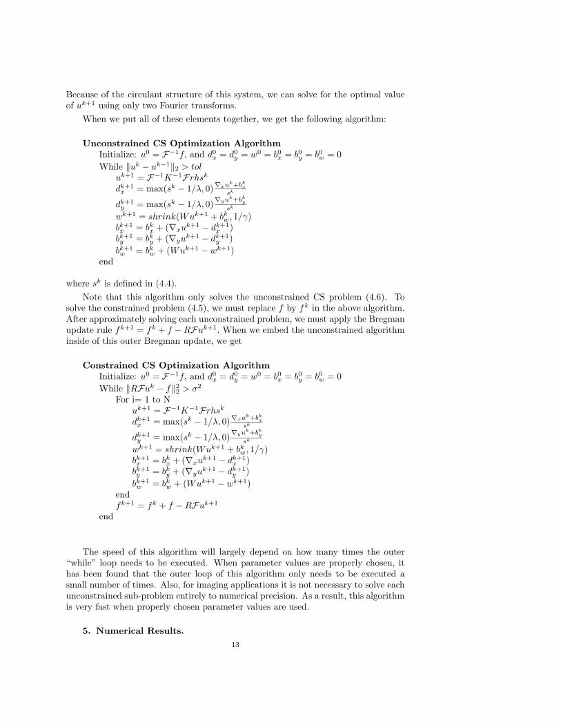
The speed of this algorithm will largely depend on how many times the outer“while” loop needs to be executed. When parameter values are properly chosen, ithas been found that the outer loop of this algorithm only needs to be executed asmall number of times. Also, for imaging applications it is not necessary to solve eachunconstrained sub-problem entirely to numerical precision. As a result, this algorithmis very fast when properly chosen parameter values are used.

5. Numerical Results.13

5.1. TV Denoising Results. We will now examine the efficiency of the splitBregman approach using time trials. The split Bregman algorithm was implementedin C++, and compiled on a UNIX platform using the g++ compiler. Time trials weregenerated on an Intel Core 2 Duo desktop PC (E6850, 3.00 GHz).

We tested our method on two images: The first was a 256× 256 synthetic imageof two overlapping squares. The second was a 512× 512 representation of the famoustest image “Lena.” Both images were contaminated with noise (σ = 15). Denoisingparameters were µ = .05, λ = 0.1 for both images. In general, we have found thatchoosing λ = 2µ usually results in good convergence. Iterations were terminatedwhen the condition ‖uk − uk−1‖/‖uk‖ < 5 ∗ 10−3 was met. Results of time trialsfor the isotropic ROF algorithm are shown in table 5.1. For comparison, we alsoreport the computation time of a graph-cuts based solver [29, 12], which minimizesan anisotropic TV functional using either a 4-neighbor stencil, or a less anisotropic16-point stencil. Note that in addition to outperforming the graph cuts algorithm interms of speed, the Split Bregman method can minimize the isotropic functional, andis thus less likely to introduce artifacts into the image.

Table 5.1ROF Computation Times (sec)

Image Split Bregman Graph Cuts(4 point) Graph Cuts(16 point)256× 256 Blocks 0.0732 0.214 0.468512× 512 Lena 0.2412 0.709 1.51

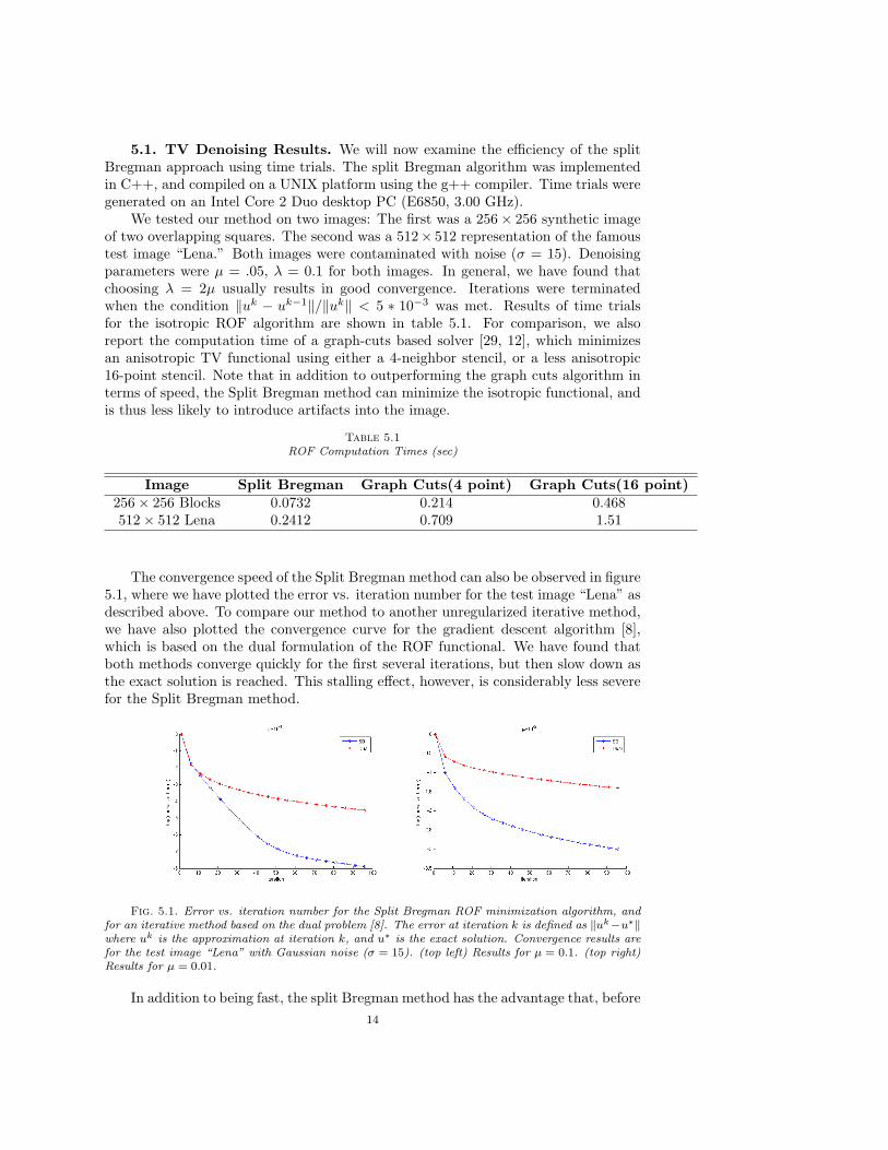
The convergence speed of the Split Bregman method can also be observed in figure5.1, where we have plotted the error vs. iteration number for the test image “Lena” asdescribed above. To compare our method to another unregularized iterative method,we have also plotted the convergence curve for the gradient descent algorithm [8],which is based on the dual formulation of the ROF functional. We have found thatboth methods converge quickly for the first several iterations, but then slow down asthe exact solution is reached. This stalling effect, however, is considerably less severefor the Split Bregman method.

Fig. 5.1. Error vs. iteration number for the Split Bregman ROF minimization algorithm, andfor an iterative method based on the dual problem [8]. The error at iteration k is defined as ‖uk−u∗‖where uk is the approximation at iteration k, and u∗ is the exact solution. Convergence results arefor the test image “Lena” with Gaussian noise (σ = 15). (top left) Results for µ = 0.1. (top right)Results for µ = 0.01.

In addition to being fast, the split Bregman method has the advantage that, before14

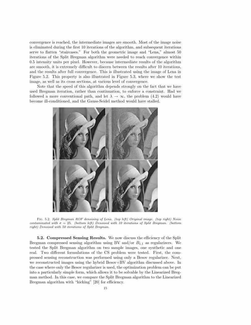
convergence is reached, the intermediate images are smooth. Most of the image noiseis eliminated during the first 10 iterations of the algorithm, and subsequent iterationsserve to flatten “staircases.” For both the geometric image and “Lena,” almost 50iterations of the Split Bregman algorithm were needed to reach convergence within0.5 intensity units per pixel. However, because intermediate results of the algorithmare smooth, it is extremely difficult to discern between the results after 10 iterations,and the results after full convergence. This is illustrated using the image of Lena inFigure 5.2. This property is also illustrated in Figure 5.3, where we show the testimage, as well as its cross sections, at various level of convergence.

Note that the speed of this algorithm depends strongly on the fact that we haveused Bregman iteration, rather than continuation, to enforce a constraint. Had wefollowed a more conventional path, and let λ → ∞, the problem (4.2) would havebecome ill-conditioned, and the Gauss-Seidel method would have stalled.

Fig. 5.2. Split Bregman ROF denoising of Lena. (top left) Original image. (top right) Noisecontaminated with σ = 25. (bottom left) Denoised with 10 iterations of Split Bregman. (bottomright) Denoised with 50 iterations of Split Bregman.

5.2. Compressed Sensing Results. We now discuss the efficiency of the SplitBregman compressed sensing algorithm using BV and/or B1,1 as regularizers. Wetested the Split Bregman algorithm on two sample images, one synthetic and onereal. Two different formulations of the CS problem were tested. First, the com-pressed sensing reconstruction was performed using only a Besov regularizer. Next,we reconstructed images using the hybrid Besov+BV algorithm discussed above. Inthe case where only the Besov regularizer is used, the optimization problem can be putinto a particularly simple form, which allows it to be solvable by the Linearized Breg-man method. In this case, we compare the Split Bregman algorithm to the LinearizedBregman algorithm with “kicking” [20] for efficiency.

15

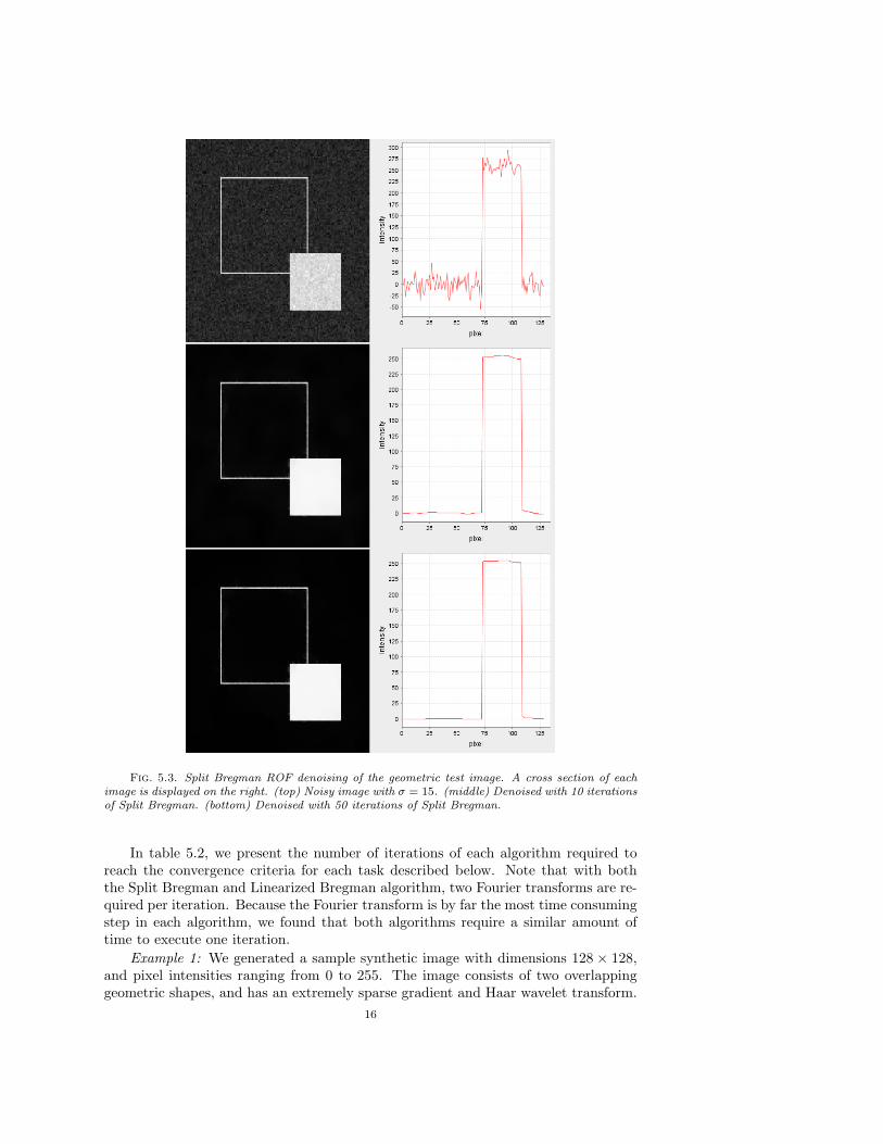
Fig. 5.3. Split Bregman ROF denoising of the geometric test image. A cross section of eachimage is displayed on the right. (top) Noisy image with σ = 15. (middle) Denoised with 10 iterationsof Split Bregman. (bottom) Denoised with 50 iterations of Split Bregman.

In table 5.2, we present the number of iterations of each algorithm required toreach the convergence criteria for each task described below. Note that with boththe Split Bregman and Linearized Bregman algorithm, two Fourier transforms are re-quired per iteration. Because the Fourier transform is by far the most time consumingstep in each algorithm, we found that both algorithms require a similar amount oftime to execute one iteration.

Example 1: We generated a sample synthetic image with dimensions 128 × 128,and pixel intensities ranging from 0 to 255. The image consists of two overlappinggeometric shapes, and has an extremely sparse gradient and Haar wavelet transform.

16

The synthetic image has signal in both its real and imaginary components, howeverfor display purposes we show the absolute value of the image. For our first test, nonoise was added to the CS data. The objective of this test was to recover the exactimage using only 50% of the k -space data (sampled at random). The algorithm wasrun until ‖Fu−fk‖2/1282 < 10−3. For the second test, the CS data was contaminatedwith noise (σ = 25), and each algorithm was run until the stopping criteria ‖Fu −fk‖2/1282 < σ was met.

Example 2: To demonstrate the effectiveness of the split Bregman method inmedical imaging, we tested the algorithm on real MRI data. For this purpose, weused a cross-sectional image of a saline phantom. In the original image acquisition,the entire k -space was sampled. To generate the CS data, we randomly and uniformlyselected 30% of the k -space samples. Note that, while ideal for compressed sensing,this type of sampling is not practical for most MRI applications. This is becausemost pulse sequences acquire k -space data in some sort of geometric pattern, such asa spiral [18, 24, 16]. Because the focus of this paper is on numerics, and not on thedetails of image acquisition, we choose uniform random sampling for simplicity.

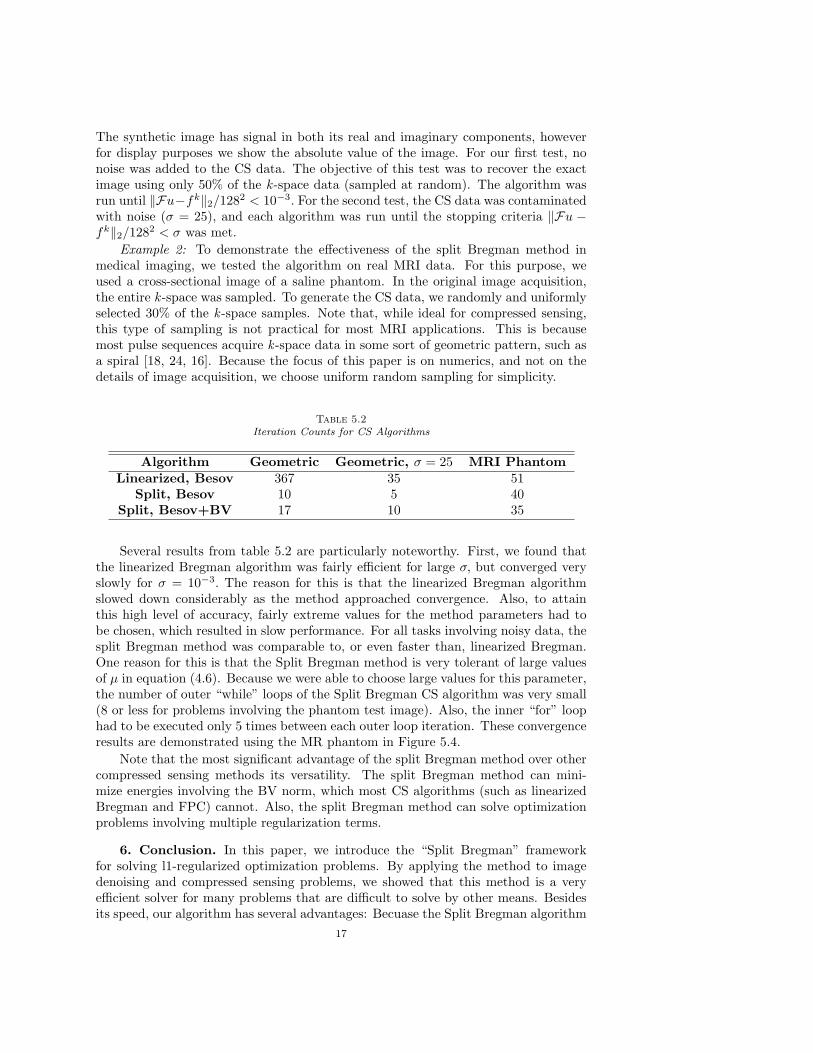
Table 5.2Iteration Counts for CS Algorithms

Algorithm Geometric Geometric, σ = 25 MRI PhantomLinearized, Besov 367 35 51

Split, Besov 10 5 40Split, Besov+BV 17 10 35

Several results from table 5.2 are particularly noteworthy. First, we found thatthe linearized Bregman algorithm was fairly efficient for large σ, but converged veryslowly for σ = 10−3. The reason for this is that the linearized Bregman algorithmslowed down considerably as the method approached convergence. Also, to attainthis high level of accuracy, fairly extreme values for the method parameters had tobe chosen, which resulted in slow performance. For all tasks involving noisy data, thesplit Bregman method was comparable to, or even faster than, linearized Bregman.One reason for this is that the Split Bregman method is very tolerant of large valuesof µ in equation (4.6). Because we were able to choose large values for this parameter,the number of outer “while” loops of the Split Bregman CS algorithm was very small(8 or less for problems involving the phantom test image). Also, the inner “for” loophad to be executed only 5 times between each outer loop iteration. These convergenceresults are demonstrated using the MR phantom in Figure 5.4.

Note that the most significant advantage of the split Bregman method over othercompressed sensing methods its versatility. The split Bregman method can mini-mize energies involving the BV norm, which most CS algorithms (such as linearizedBregman and FPC) cannot. Also, the split Bregman method can solve optimizationproblems involving multiple regularization terms.

6. Conclusion. In this paper, we introduce the “Split Bregman” frameworkfor solving l1-regularized optimization problems. By applying the method to imagedenoising and compressed sensing problems, we showed that this method is a veryefficient solver for many problems that are difficult to solve by other means. Besidesits speed, our algorithm has several advantages: Becuase the Split Bregman algorithm

17

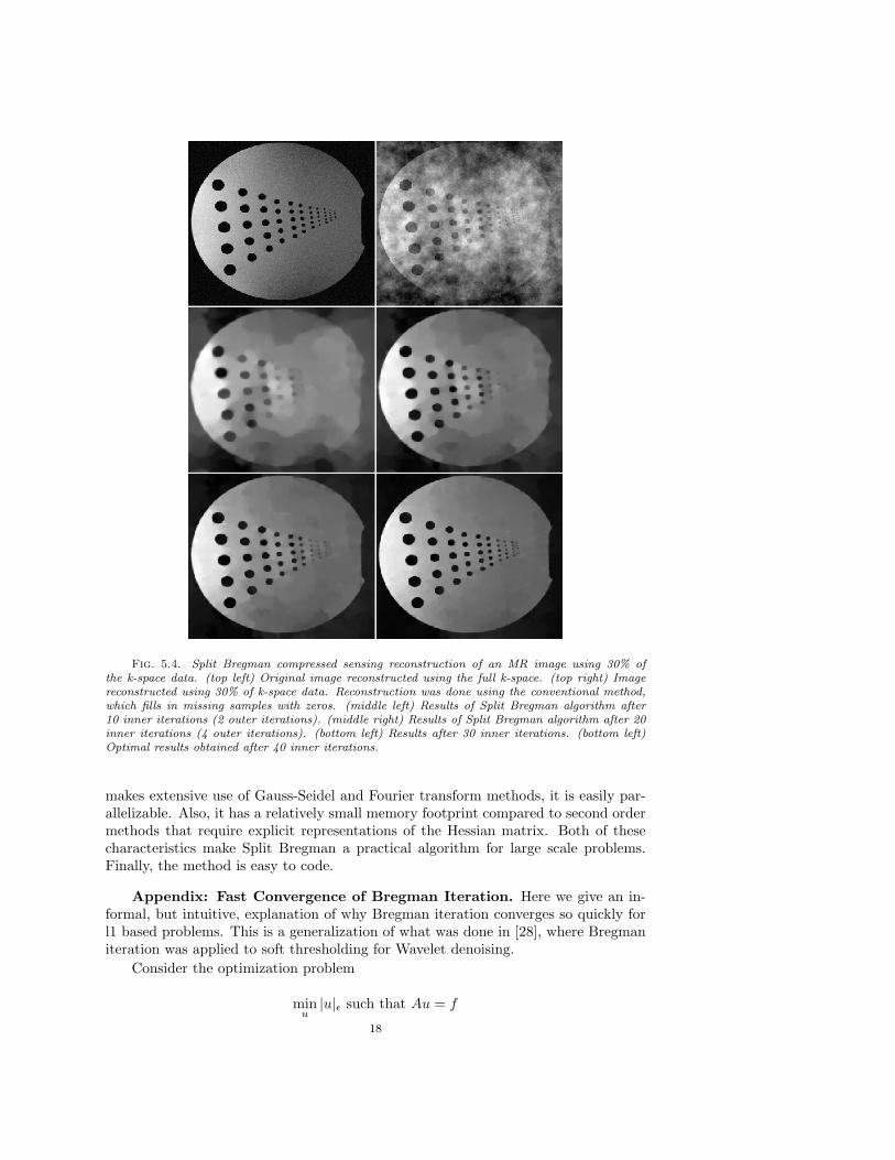
Fig. 5.4. Split Bregman compressed sensing reconstruction of an MR image using 30% ofthe k-space data. (top left) Original image reconstructed using the full k-space. (top right) Imagereconstructed using 30% of k-space data. Reconstruction was done using the conventional method,which fills in missing samples with zeros. (middle left) Results of Split Bregman algorithm after10 inner iterations (2 outer iterations). (middle right) Results of Split Bregman algorithm after 20inner iterations (4 outer iterations). (bottom left) Results after 30 inner iterations. (bottom left)Optimal results obtained after 40 inner iterations.

makes extensive use of Gauss-Seidel and Fourier transform methods, it is easily par-allelizable. Also, it has a relatively small memory footprint compared to second ordermethods that require explicit representations of the Hessian matrix. Both of thesecharacteristics make Split Bregman a practical algorithm for large scale problems.Finally, the method is easy to code.

Appendix: Fast Convergence of Bregman Iteration. Here we give an in-formal, but intuitive, explanation of why Bregman iteration converges so quickly forl1 based problems. This is a generalization of what was done in [28], where Bregmaniteration was applied to soft thresholding for Wavelet denoising.

Consider the optimization problem

minu|u|ε such that Au = f

18

Fig. 5.5. Synthetic image recovered from 50% of k-space data. The k-space data was contam-inated with noise (σ = 15) prior to recovery. (top left) Original image reconstructed using the fullk-space. (top right) Image reconstructed using 50% of k-space data. Reconstruction was done usingthe conventional method, which fills in missing samples with zeros. (bottom left) CS reconstructionusing only the Besov regularizer. (bottom right) CS results using the hybrid TV+Besov regularizer.Note the superiority of the results when the hybrid regularizer is used.

where

|u|ε =∑i

√u2j + ε

is a “smoothed out” variant of the l1 norm. We will need this smoothness to performthe analysis below. The Bregman update rule for this problem is

pk+1 − pk +AT (Auk+1 − f) = 0(6.1)

Now, because J(·) = | · |ε is convex, and pk and pk+1 are gradients of this functionalat uk and uk+1, the mean value theorem tells us that

pk+1 − pk = Dk+ 12 (uk+1 − uk)

where Dk+ 12 is a diagonal matrix such that

Dk+ 1

2i,i = ε

((uk+

12

i )2 + ε)−3/2

for some uk+12 between uk and uk+1.

Applying this formula to (6.1) yields

Dk+ 12 (uk+1 − uk) +AT (Auk+1 − f) = 0

19

We now let Qk+12 = (Dk+ 1

2 )−1, multiply by AQk+12 , and rearrange to get

Auk+1 − f =(I +AQk+

12AT

)−1 (Auk − f

)(6.2)

This equation gives us some insight into why Bregman iteration behaves as itdoes. When u

k+ 12

i is large compared to ε, which occurs at “spikes” (or edges in the

BV case), Qk+12

i,i is large, and uki converges rapidly. Small values of uk take moreiterations to settle down. An important result of this is that for problems with shocksor edges, Bregman iteration puts these features in the right place almost immediately,unlike the continuation based method [27]. Resolving discontinuities is usually themost difficult part of any imaging task, and Bregman iteration is extremely well suitedfor this task.

Acknowledgment. We thank Jie Zheng for his helpful discussions regardingMR image processing. This publication was made possible by the support of theNational Science Foundation’s GRFP program, as well as ONR grant N000140710810and the Department of Defense.

REFERENCES

[1] R. Baraniuk and P. Steeghs. Compressive radar imaging. Radar Conference, 2007 IEEE, pages128–133, 2007.

[2] Stephen Boyd and Lieven Vandenberghe. Convex Optimization. Cambridge University Press,2004.

[3] Y. Boykov, O. Veksler, and R. Zabih. Fast approximate energy minimization via graph cuts.Pattern Analysis and Machine Intelligence, 23:1222 – 1239, 2005.

[4] L Bregman. The relaxation method of finding the common points of convex sets and itsapplication to the solution of problems in convex optimization. USSR ComputationalMathematics and Mathematical Physics, 7:200–217, 1967.

[5] JF Cai, S. Osher, and Z Shen. Linearized Bregman iterations for compressed sensing. UCLACAM Report, 08-06.

[6] E. J. Candes and J. Romberg. Signal recovery from random projections. Proceedings of SPIEComputational Imaging III, 5674:76 — 86, 2005.

[7] E. J. Candes, J. Romberg, and T.Tao. Robust uncertainty principles: Exact signal reconstruc-tion from highly incomplete frequency information. IEEE Trans. Inform. Theory, 52:489– 509, 2006.

[8] A. Chambolle. Total variation minimization and a class of binary mrf models. In EnergyMinimization Methods in Computer Vision and Pattern Recognition, pages 136 – 152.Springer, 2005.

[9] Tony F. Chan, Gene H. Golub, and Pep Mulet. A nonlinear primal-dual method for totalvariation-based image restoration. In ICAOS ’96 (Paris, 1996),, volume 219, pages 241–252, Berlin, Germany / Heidelberg, Germany / London, UK / etc., 1996. Springer-Verlag.

[10] J Darbon and M Sigelle. A fast and exact algorithm for total variation minimization. IbPRIA,3522:351–359, 2005.

[11] D Donoho. Compressed sensing. Information Theory, IEEE Transactions on, 52:1289–1306,2006.

[12] D. Goldfarb and W. Yin. Parametric maximum flow algorithms for fast total variation mini-mization. CAAM technical report, TR07-09, 2008.

[13] Elaine Hale, Wotao Yin, and Yin Zhang. A fixed-point continuation method for l1-regularizedminimization with applications to compressed sensing. CAAM Technical Report, TR07,2007.

[14] Lin He, Ti-Chiun Chang, and Stanley Osher. Mr image reconstruction from sparse radialsamples by using iterative refinement procedures. Proceedings of the 13th annual meetingof ISMRM, page 696, 2006.

[15] Y Li and F Santosa. An affine scaling algorithm for minimizing total variation in image enhance-ment. Tech Repost 12/94, Center for theory and simulation in science and engineering,Cornell University, (TR94-1470):24, 1994.

20

[16] M Lustig, D Donoho, and J Pauly. Sparse mri: The application of compressed sensing for rapidmr imaging. Magnetic Resonance in Medicine, 58:1182–1195, 2007.

[17] M Lustig, J.H. Lee, D.L. Donoho, and J.M. Pauly. Faster imaging with randomly perturbedundersampled spirals and l1 reconstruction. Proc. Of the ISMRM, 2005.

[18] GL Marseille, R de Beer, M Fuderer, AF Mehlkopf, and D van Ormondt. Nonunifom phase-encode distributions for MRI scan-time reduction. J Magn Reson, 111:70–75, 1996.

[19] J Nocedal and S. Wright. Numerical Optimization. Springer Verlag, 2006.[20] A Osher, Y Mao, B Dong, and W Yin. Fast linearized Bregman iterations for compressed

sensing and sparse denoising. UCLA CAM Report, 08-37.[21] Stanley Osher, Martin Burger, Donald Goldfarb, Jinjun Xu, and Wotao Yin. An iterative

regularization method for total variation-based image restoration. MMS, 4:460–489, 2005.[22] L Rudin, S Osher, and E Fatemi. Nonlinear total variation based noise removal algorithms.

Physica. D., 60:259–268, 1992.[23] Kim S, K Koh, M Lustig, S Boyd, and D Gerinvesky. A method for large-scale l1-regularized

least squares problems with applications in signal processing and statistics. Tech. Report,Dept. of Electrical Engineering, Stanford University, 2007.

[24] J Trzasko, A Manduca, and E Borisch. Sparse mri reconstruction via multiscale l0-continuation.Statistical Signal Processing, 26–29:176 – 180, 2007.

[25] C. Vogel. A multigrid method for total variation-based image denoising. Computation andControl IV, Progress in Systems and Control Theory, 20, Birkhauser, 1995.

[26] C. R. Vogel and M. E. Oman. Iterative methods for total variation denoising. SIAM Journalon Scientific Computing, 17(1):227–238, 1996.

[27] Y Wang, W Yin, and Y Zhang. A fast algorithm for image deblurring with total variationregularization. CAAM Technical Reports, 2007.

[28] J Xu and S Osher. Iterative regularization and nonlinear inverse scale space applied to wavelet-based denoising. IEEE Transactions on Image Processing, 16:534–544, February 2007.

[29] W. Yin. Pgc: A preflow-push based graph-cut solver. version 2.32.[30] W Yin, S Osher, D Goldfarb, and J Darbon. Bregman iterative algorithms for l1-minimization

with applications to compressed sensing. Siam J. Imaging Science, 1:142–168, 2008.

21