The Spearman and Kendall rank correlationcoefficients between intuitionistic fuzzy sets

Eulalia Szmidt and Janusz Kacprzyk

Systems Research Institute Polish Academy of Sciences, ul.Newelska 6, 01-447 Warsaw, PolandWIT – Warsaw School of Information Technology ul. Newelska 6, 01-447 Warsaw, Poland

{szmidt, kacprzyk }@ibspan.waw.pl

Abstract

This paper is a continuation of our previous work onPearson’s coefficientr and we discuss here the conceptof theSpearman correlation coefficientand theKendallcorrelation coefficientbetween Atanassov’s intuitionis-tic fuzzy sets (A-IFSs, for short) to measure the degreeof association between the A-IFSs when the assumptionthat the data distributions are normal is not valid or whendata are in the form of ranks.

Keywords: Intuitionistic fuzzy sets, correlation, theSpearman correlation coefficient, the Kendall correla-tion coefficient

1. Introduction

It is often important to know the relationships betweenrelevant variables while building models describing aprocess or a system. The Pearson correlation coefficientr measuring a linear relationship between the variablesis one of the most frequently used tools in statistics (cf.Rodgers and Nicewander [14]). Generally, correlationindicates how well two normally distributed variablesmove together in a linear way (Rodgers and Nicewan-der [14], Aczel [1]). When the assumption about thenormal distributions of the variables considered is notvalid or the data are in the form of ranks, we use othermeasures of the degree of association between two vari-ables, namely theSpearman rank correlation coefficientrs (e.g., Aczel [1]) or theKendall τ correlation coeffi-cient(Kendall [9]).

As Zadeh has observed [37], [38], most of informa-tion relevant to probabilistic analyzes is imprecise, andthere is imprecision and fuzziness not only in probabil-ities, but also in events, relations and properties. In thiscontext, the probabilistic concepts should also be ex-tended to fuzzy models and their generalizations. Theanalysis of relationships between the A-IFSs, which area generalization of fuzzy sets, seems to be of a vi-tal importance, too. We have already discussed in de-tail the Pearson correlation coefficientr (Szmidt andKacprzyk [32]. In this paper we jointly discuss theSpearman rank correlation coefficientrs (Szmidt andKacprzyk [33]) and theKendallτ correlation coefficientto find and indicate some common properties and differ-ences.

Both theSpearman rank correlation coefficientandtheKendallτ correlation coefficientfor the A-IFSs are

a generalization of their crisp counterparts (it boils downto them, and preserve the same properties each).

Moreover, both correlation coefficients take into ac-count all three terms describing the A-IFS, i.e., the mem-bership values, non-membership values, and hesitationmargins. We show that each term plays an importantrole in data analysis and decision making.

2. A Brief Introduction to Intuitionistic Fuzzy Sets

One of the possible generalizations of a fuzzy set inX(Zadeh [36]), given by

A′

= {< x, µA′ (x) > |x ∈ X} (1)

whereµA′ (x) ∈ [0, 1] is the membership function of

the fuzzy setA′

, is Atanassov’s intuitionistic fuzzy setA (Atanassov [2], [3]), namely:

A = {< x, µA(x), νA(x) > |x ∈ X} (2)

where: µA : X → [0, 1] andνA : X → [0, 1] suchthat 0<µA(x) + νA(x)<1, andµA(x), νA(x) ∈ [0, 1]denote the degree of membership and a degree of non-membership ofx ∈ A, respectively, and thehesitationmarginof x ∈ A is:

πA(x) = 1 − µA(x) − νA(x) (3)

The πA(x) expresses a lack of knowledge of whetherx belongs toA or not (Atanassov [3]); obviously,0<πA(x)<1, for eachx ∈ X ;

The hesitation margin turns out to be important whileconsidering the distances (Szmidt and Kacprzyk [16],[18], [25], entropy (Szmidt and Kacprzyk [20], [27]),similarity (Szmidt and Kacprzyk [28]) for the A-IFSs,etc. i.e., the measures that play a crucial role in virtuallyall information processing tasks. The hesitation marginis shown to be indispensable also in the ranking of in-tuitionistic fuzzy alternatives as it indicates how reliable(sure) information represented by an alternative is (cf.Szmidt and Kacprzyk [29], [30]).

The use of A-IFSs instead of fuzzy sets implies theintroduction of additional degrees of freedom (non-memberships and hesitation margins) into the set de-scription. Such a generalization of fuzzy sets gives usan additional possibility to represent imperfect knowl-edge which may lead to describing many real problemsin a more adequate way. This is confirmed by successful

EUSFLAT-LFA 2011 July 2011 Aix-les-Bains, France

© 2011. The authors - Published by Atlantis Press 521

Figure 1: Geometrical representation

applications of A-IFSs to group decision making, ne-gotiations, voting and other situations are presented inSzmidt and Kacprzyk [15], [17], [19], [21], [22], [23],[24], [26], [31], Szmidt and Kukier [34], [35].

2.1. A geometrical representation

One of possible geometrical representations of anintuitionistic fuzzy sets is given in Figure 1 (cf.Atanassov [3]). It is worth noticing that although weuse a two-dimensional figure (which is more convenientto draw in our further considerations), we still adopt ourapproach (e.g., Szmidt and Kacprzyk [18], [25], [20],[27]), [28]) taking into account all three terms (member-ship, non-membership and hesitation margin values) de-scribing an intuitionistic fuzzy set. Any element belong-ing to an intuitionistic fuzzy set may be represented in-side anMNO triangle. In other words, theMNO trian-gle represents the surface where the coordinates of anyelement belonging to an A-IFS can be represented. Eachpoint belonging to theMNO triangle is described by thethree coordinates:(µ, ν, π). PointsM andN representthe crisp elements. PointM(1, 0, 0) represents elementsfully belonging to an A-IFS asµ = 1, and may be seenas the representation of the ideal positive element. PointN(0, 1, 0) represents elements fully not belonging to anA-IFS asν = 1, i.e. can be viewed as the ideal nega-tive element. PointO(0, 0, 1) represents elements aboutwhich we are not able to say if they belong or not be-long to an A-IFS (the intuitionistic fuzzy indexπ = 1).Such an interpretation is intuitively appealing and pro-vides means for the representation of many aspects ofimperfect information. SegmentMN (whereπ = 0)represents elements belonging to the classic fuzzy sets(µ + ν = 1). For example, pointx1(0.2, 0.8, 0) (Figure1), like any element from segmentMN represents anelement of a fuzzy set. A line parallel toMN describesthe elements with the same values of the hesitation mar-gin. In Figure 1 we can see pointx3(0.5, 0.1, 0.4) repre-senting an element with the hesitation margin equal 0.4,and pointx2(0.2, 0, 0.8) representing an element withthe hesitation margin equal 0.8. The closer a line that is

parallel toMN is toO, the higher the hesitation margin.

3. Correlation, the Spearman and Kendall RankCorrelation Coefficients between crisp sets

The correlation coefficient (Pearson’sr) between twovariables is a measure of the linear relationship betweenthem.

The correlation coefficient is 1 in the case of a positive(increasing) linear relationship, -1 in the case of a nega-tive (decreasing) linear relationship, and some value be-tween -1 and 1 in all other cases. The closer the coef-ficient is to either -1 or 1, the stronger the correlationbetween the variables.

Definition 1 Let (X1, Y1), (X2, Y2), . . . ,(Xn, Yn) be arandom sample of sizen from a joint probability densityfunctionfX,Y (x, y), let X andY be the sample meansof variablesX andY , respectively, then the sample cor-relation coefficientr(X, Y ) is given as (e.g., [14]):

r(A, B) =

n∑

i=1

(xi − X)(yi − Y )

(n∑

i=1

(xi − X)2n∑

i=1

(yi − Y )2)0.5

(4)

where:X = 1n

n∑

i=1

xi, Y = 1n

n∑

i=1

yi.

When the assumption that the data distributions arenormal is not valid or when data are in the form of ranks,we may use theSpearman rank correlation coefficientortheKendall rank correlation coefficient.

Definition 2 Let (X1, Y1), (X2, Y2), . . . , (Xn, Yn) bea random sample of sizen. To compute theSpearmancorrelation coefficientwe rank all the observations of thefirst variable. Next, we independently rank the valuesof the second variable. TheSpearman rank correlationcoefficientis thePearson correlation coefficientappliedto the ranksR, namely (e.g., Aczel [1]):

r(A, B) =n

∑

i=1

(R(xi)−1

2(n+1))(R(yi)−

1

2(n+1))/

/(

n∑

i=1

(R(xi)−1

2(n+1))2

n∑

i=1

(R(yi)−1

2(n+1))2)0.5

(5)

and in (5) the average values forX andY are the sameand equal to0.5(n + 1).

When there are not two values ofX or two values ofYwith the same rank (so called ties), there is an easier wayto compute the Spearman correlation coefficient, namely(e.g., Aczel [1], Myers and Well [11]):

rs = 1 −

6n∑

i=1

d2i

n(n2 − 1)(6)

wheredi, i = 1, . . . , n are the differences in the ranksof xi andyi: di = R(xi) − R(yi). If there are ties (two

522

values ofX or two values ofY with the same rank), butthe number of ties is small compared withn, (6) is stilluseful (cf. Aczel [1]).

The Spearman correlation coefficient fulfills the re-quirements of the correlation measures. As (6) was ob-tained from the Pearson coefficient for ranks, it fulfillsthe same properties as the Pearson coefficient (see e.g.,Rodgers and Nicewander [14]), i.e.:

1. rs(A, B) = rs(B, A),2. If A = B thenrs(A, B) = 1,3. |rs(A, B)| ≤ 1.

When the variablesX andY are perfectly positivelyrelated, i.e., whenX increases wheneverY increases,rs is equal to 1. WhenX andY are perfectly negativelyrelated, i.e., whenX increases wheneverY decreases,rs is equal to -1.rs is equal to zero when there is norelation betweenX andY . Values between -1 and 1 givea relative indication of the degree of association betweenX andY . In other words,−1 ≤ rs ≤ 1.

Definition 3 (e.g., Nelsen [12]) Let(x1, y1), (x2, y2),. . . , (xn, yn) be a set of joint observations from two ran-dom variablesX andY respectively, such that all thevalues of(xi) and(yi) are unique. Any pair of observa-tions(xi, yi) and(xj , yj) are said to be concordant if theranks for both elements agree: that is, if bothxi > xj

and yi > yj or if both xi < xj and yi < yj . Theyare said to be discordant, ifxi > xj andyi < yj or ifxi < xj andyi > yj . If xi = xj or yi = yj , the pair isneither concordant, nor discordant.

For n observations, (i.e.,(i, j) ∈ {1, . . . , n}2) thenumber of concordantC, discordantD, tied parsT inX , and tied pairsU in Y is denoted:

C = |{(i, j)|xi < xj andyi < yj}| (7)

D = |{(i, j)|xi < xj andyi > yj}| (8)

T = |{(i, j)|xi = xj}| (9)

U = |{(i, j)|yi = yj}| (10)

The Kendallτ coefficient is defined as [9]:

τ =C − D

12 n(n − 1)

(11)

where:C - number of concordant pairs;D - number ofdiscordant pairs, and

|τ | ≤ 1

For the perfect agreement between the two rankings(i.e., all pairs are concordant) the coefficient has value1. For the perfect disagreement between the two rank-ings (i.e., all pairs are discordant) the coefficient hasvalue -1. All other arrangements produce the value ofτ between -1 and 1 (increasing values imply increasingagreement between the rankings). For completely inde-pendent rankings, the coefficient has value 0.

If two values ofX or two values ofY with the samerank (so called ties) occur, the following formula is used

(Kendall [9]):

τb =c − D

√

12 (n(n − 1) − T

√

12 )n(n − 1) − U

(12)

where: T - number of ties inX (number of pairs forwhich xi = xj ; U - number of ties inY (number ofpairs for whichyi = yj .

4. Correlation, and the Spearman and KendallRank Correlation Coefficients between theA-IFSs

In Szmidt and Kacprzyk [32] we proposed a correlationcoefficient for two A-IFSs,A andB, so that we couldexpress not only a relative strength but also a positiveor negative relationship betweenA and B. We tookinto account all three terms describing an A-IFSs (themembership, non-membership values and the hesitationmargins) because each of them influences the results (cf.[32].

Suppose that we have a random samplex1, x2, . . . , xn ∈ X with a sequence of paired data[(µA(x1),νA(x1),πA(x1)), (µB(x1),νB(x1),πB(x1))],[(µA(x2), νA(x2), πA(x2)), (µB(x2), νB(x2),πB(x2))], . . ., [(µA(xn), νA(xn), πA(xn)), (µB(xn),νB(xn), πB(xn))] which correspond to the member-ship values, non-memberships values and hesitationmargins of the A-IFSsA and B defined onX , thenthe correlation coefficientrA−IF S(A, B) is given byDefinition 4.

Definition 4 The correlation coefficientrA−IF S(A, B)between two A-IFSs,A and B in X , is (Szmidt andKacprzyk [32]):

rA−IF S(A, B) =1

3(r1(A, B) + r2(A, B) + r3(A, B))

(13)where

r1(A, B) =

n∑

i=1

(µA(xi) − µA)(µB(xi) − µB)/ (14)

/(

n∑

i=1

(µA(xi) − µA)2)0.5(

n∑

i=1

(µB(xi) − µB)2)0.5

r2(A, B) =n

∑

i=1

(νA(xi) − νA)(νB(xi) − νB)/ (15)

/(

n∑

i=1

(νA(xi) − νA)2)0.5(

n∑

i=1

(νB(xi) − νB)2)0.5

r3(A, B) =

n∑

i=1

(πA(xi) − πA)(πB(xi) − πB)/ (16)

/(n

∑

i=1

(πA(xi) − πA)2)0.5(n

∑

i=1

(πB(xi) − πB)2)0.5

523

where: µA = 1n

n∑

i=1

µA(xi), µB = 1n

n∑

i=1

µB(xi),

νA = 1n

n∑

i=1

νA(xi), νB = 1n

n∑

i=1

νB(xi), πA =

1n

n∑

i=1

πA(xi), πB = 1n

n∑

i=1

πB(xi),

The proposed correlation coefficient (13) depends ontwo factors: the amount of information expressed by themembership and non-membership degrees (14)–(15),and the reliability of information expressed by the hesi-tation margins (16).Remark: Analogously as for the crisp and fuzzy data,rA−IF S(A, B) makes sense for the A-IFS type variableswhose values vary. If, for instance, the temperature isconstant and the amount of ice cream sold is the same,then it is impossible to conclude about their relationship(as, from the mathematical point of view, we avoid zeroin the denominator).

The correlation coefficientrA−IF S(A, B) (13) ful-fills the following properties:

1. rA−IF S(A, B) = rA−IF S(B, A),2. If A = B thenrA−IF S(A, B) = 1,3. |rA−IF S(A, B)| ≤ 1.

The above properties are not only fulfilled by thecorrelation coefficientrA−IF S(A, B) (13) but also byall of its three components (14)–(16).Remark: It is should be emphasized thatrA−IF S(A, B) = 1 occurs not only forA = Bbut also in the cases of a perfect linear correlation of thedata (the same concerns each component (14)–(16)).

From Definition 4, we immediately obtain theSpear-man rank correlation coefficientbecause it is the usual(Pearson) correlation coefficient applied to the ranks.

Definition 5 The Spearman rank correlation coefficientis defined as:

rsA−IF S=

1

3(rs1

+ rs1+ rs1

) (17)

where rsi, i = 1, . . . , 3 are the Spearman rank cor-

relation coefficients betweenA andB with respect totheir membership function, non-membership function,and hesitation margin, given as:

rs1= 1 −

6n∑

i=1

d21i

n(n2 − 1)(18)

where d1i, i = 1, . . . , n are the differences in theranks with respect to the membership functions:d1i =R(µA(xi)) − R(µB(xi)),

rs2= 1 −

6n∑

i=1

d22i

n(n2 − 1)(19)

whered2i, i = 1, . . . , n are the differences in the rankswith respect to the non-membership functions:d2i =R(νA(xi)) − R(νB(xi)), and

rs2= 1 −

6n∑

i=1

d23i

n(n2 − 1)(20)

Table 1: Example 1 - calculations of (18)Patient No. µA R(µA) µB R(µB) d1 d2

1

1 0.1 1 0.2 1 0 02 0.3 3 0.42 2 1 13 0.39 4 0.5 3 1 14 0.42 5 0.53 4 1 15 0.2 2 0.65 5 -3 9

Table 2: Example 1 - calculations of (19)Patient No. νA R(νA) νB R(νB) d2 d2

2

1 0.05 1 0.12 1 0 02 0.15 2 0.28 3 -1 13 0.3 3 0.31 5 -2 44 0.48 4 0.29 4 0 05 0.72 5 0.18 2 3 9

where d3i, i = 1, . . . , n are the differences in theranks with respect to the hesitation margins:d3i =R(πA(xi)) − R(πB(xi)).

Obviously, for theSpearman rank correlation(17) thesame properties as for thePearson correlations coeffi-cientare valid, i..e.:

1. rsA−IF S(A, B) = rsA−IF S

(B, A)

2. If A = B thenrsA−IF S(A, B) = 1

3. |rsA−IF S(A, B)| ≤ 1

The separate components of theSpearman rank correla-tion (17) i.e., (18)–(20) fulfill the above properties, too.

Obviously, in the case of crisp sets,rsA−IF S(17) re-

duces tors (6).

Table 3: Example 1 - calculations of (20)Patient No. πA R(πA) πB R(πB) d3 d2

3

1 0.85 5 0.68 5 0 02 0.55 4 0.3 4 0 03 0.31 3 0.19 2 1 14 0.1 2 0.27 3 -1 15 0.08 1 0.17 1 0 0

Example 1 For instance, while administering any med-ication, an expert clinician should make decision basedon the context of the individual patient and his/her ownpast experience of the expected effect (e.g. Helgasonand Jobe [5], [6]). The effects may be positive (ex-pressed by a membership value), negative (expressed bya non-membership value), and difficult to foresee (ex-pressed by a hesitation margin), for a specific patient.Suppose that two new medicinesA andB are tested, andtheir effects on 5 patients are the following (Figure 2):

A ={(x1, 0.1, 0.05, 0.85), (x2, 0.3, 0.15, 0.55), (21)

(x3, 0.39, 0.3, 0.31), (x4, 0.42, 0.48, 0.1),

(x5, 0.2, 0.72, 0.08)}

B ={(x1, 0.2, 0.12, 0.68), (x2, 0.42, 0.28, 0.3), (22)

(x3, 0.5, 0.31, 0.19), (x4, 0.53, 0.29, 0.27),

(x5, 0.65, 0.18, 0.17)}

524

0.5

0.5 0

1

1

0.4

0.4

0.3

0.3 ) 0 , 0 , 1 ( M

) 0 , 1 , 0 ( N

0.2

0.2

0.1

0.1

0.6

0.6

0.7

0.7

0.8

0.8

0.9

0.9

values membership

valu

es

mem

bers

hip

- no

n

1 A

1 B 2 A

3 A

4 A

5 A

2 B

3 B 4 B

5 B

Figure 2: Data from Example 1

where, for example, the positive effects of medicineAon the first patient (x1) are expressed by the membershipvalue equal to 0.1, the negative effects are expressed bythe non-membership value equal to 0.05, and effects dif-ficult to forsee are expressed by the hesitation marginequal to 0.85; etc.

As the assumption of a normal distribution may beinappropriate, we use the Spearman rank correlation co-efficient to conclude about the association between thetwo medicinesA andB. Due to (17), we examine firstthe positive effects expressed byµA, andµB (Table 1)

so as to obtain the value of (18). As5

∑

i=1

d21i = 12, from

(18) we obtainrs1= 1 − ((6 ∗ 12)/(5 ∗ 24)) = 0.4.

Repeating the same calculations for the negative effectsexpressed byνA, andνB (Table 2), we obtain the valueof rs2

(19) equal to 0.3. Finally, we examine effects thatare difficult to forsee (Table 3), and obtain the value ofrs3

(20) equal to1 − ((6 ∗ 2)/(5 ∗ 24)) = 0.9. As a re-sult, from (17), we obtainrsA−IF S

= 0.53. But from thepoint of view of an expert clinician all three componentsmay seem interesting. Let us notice that in this examplethe data are such thatrs3

influences substantially the fi-nal result. If we consider a relationship betweenA andB only in the categories of the positive effects and neg-ative effects, we obtain an average relationship equal to0.5(0.4 + 0.3) = 0.35 which suggests that the relation-ship betweenA andB is not strong. On the other hand,rs3

(20) equal to 0.9 suggests that both medicines are re-lated as far as unforseen effects are concerned. It may bean important information from a medical point of view.

By showing in detail the above small example wewanted to illustrate that all three terms describing the A-IFSs, namely the membership values, non-membershipvalues, and hesitation margins are important from thepoint of view of assessing the correlation between the A-IFSs. It seems obvious as each of the term “speaks” foranother aspect of a system described via an A-IFS. Themembership values and non-memberships values repre-sent our knowledge whereas the hesitation margins rep-resent a lack of knowledge. It seems that from a point

of view of decision making we can not exclude from themodels a lack of knowledge which in real world is thesubject of equal or even more interest that “sure knowl-edge” (represented in the A-IFS models by the member-ship and non-membership values).

Now we will propose the definition of theKendallrank correlation coefficientfor the A-IFSs, and will useit to solve the same Example 1.

Definition 6 The Kendall rank correlation coefficientτA−IF S between two A-IFSs,A andB in X is definedas:

τA−IF S =1

3(τ1 + τ2 + τ3) (23)

where: τi, i = 1, . . . , 3 are the Kendall rank correla-tion coefficients betweenA andB with respect to theirmembership values, non-membership values, and hesi-tation margin values, given as:

τ1 =Cµ − Dµ

12 n(n − 1)

(24)

where: Cµ – the number of concordant pairs with re-spect to the membership values;Dµ – the number ofdiscordant pairs with respect to the membership values,i.e.:

Cµ = |{(i, j)|µA(xi)<µA(xj) andµB(xi)<µB(xj)}|(25)

Dµ = |{(i, j)|µA(xi)<µA(xj) andµB(xi)>µB(xj)}|(26)

τ2 =Cν − Dν

12 n(n − 1)

(27)

where: Cν – the number of concordant pairs with re-spect to the non-membership values;Dν – the numberof discordant pairs with respect to the non-membershipvalues, i.e.:

Cν = |{(i, j)|νA(xi)<νA(xj) andνB(xi)<νB(xj)}|(28)

Dν = |{(i, j)|νA(xi)<νA(xj) andνB(xi)>νB(xj)}|(29)

and

τ3 =Cπ − Dπ

12 n(n − 1)

(30)

where: Cπ – the number of concordant pairs with re-spect to the hesitation margins;Dπ – the number of dis-cordant pairs with respect to the hesitation margins, i.e.:

Cπ = |{(i, j)|πA(xi)<πA(xj) andπB(xi)<πB(xj)}|(31)

Dπ = |{(i, j)|πA(xi)<πA(xj) andπB(xi)>πB(xj)}|(32)

For theKendall rank correlation coefficientτ (23) be-tween the A-IFSs the same properties as for its crisp setcounterpart are valid, i..e.:

525

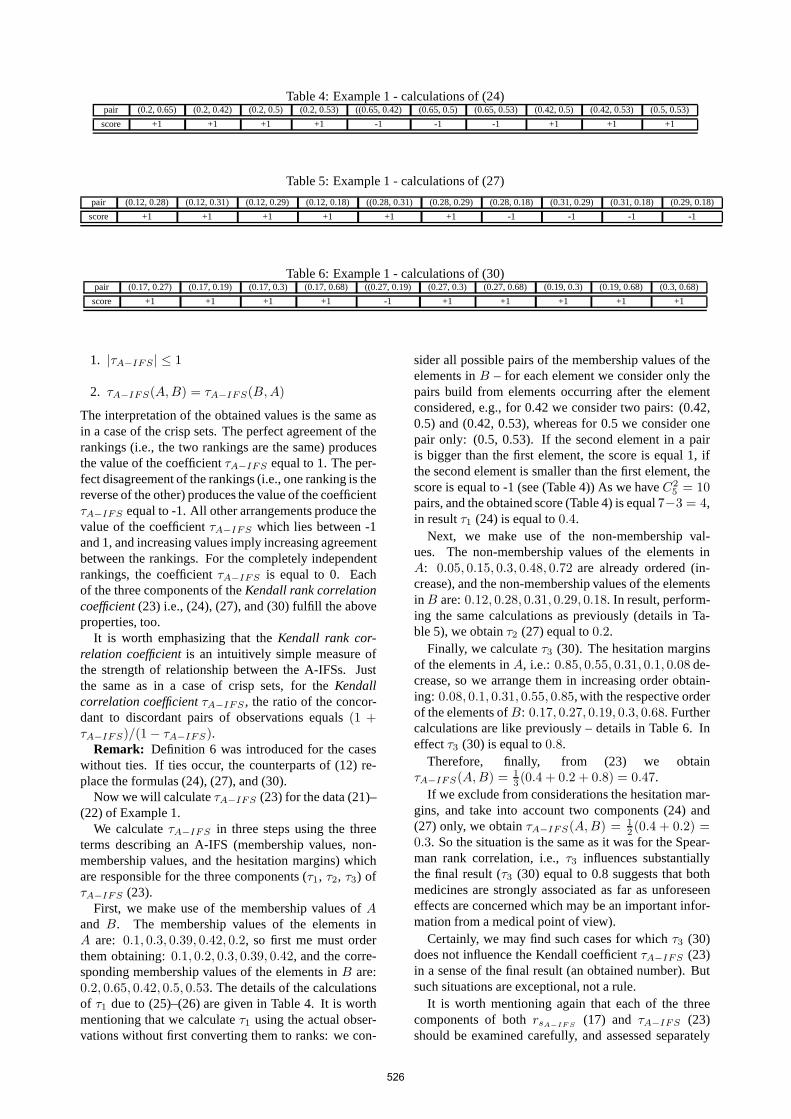
Table 4: Example 1 - calculations of (24)pair (0.2, 0.65) (0.2, 0.42) (0.2, 0.5) (0.2, 0.53) ((0.65, 0.42) (0.65, 0.5) (0.65, 0.53) (0.42, 0.5) (0.42, 0.53) (0.5, 0.53)

score +1 +1 +1 +1 -1 -1 -1 +1 +1 +1

Table 5: Example 1 - calculations of (27)

pair (0.12, 0.28) (0.12, 0.31) (0.12, 0.29) (0.12, 0.18) ((0.28, 0.31) (0.28, 0.29) (0.28, 0.18) (0.31, 0.29) (0.31, 0.18) (0.29, 0.18)

score +1 +1 +1 +1 +1 +1 -1 -1 -1 -1

Table 6: Example 1 - calculations of (30)pair (0.17, 0.27) (0.17, 0.19) (0.17, 0.3) (0.17, 0.68) ((0.27, 0.19) (0.27, 0.3) (0.27, 0.68) (0.19, 0.3) (0.19, 0.68) (0.3, 0.68)

score +1 +1 +1 +1 -1 +1 +1 +1 +1 +1

1. |τA−IF S | ≤ 1

2. τA−IF S(A, B) = τA−IF S(B, A)

The interpretation of the obtained values is the same asin a case of the crisp sets. The perfect agreement of therankings (i.e., the two rankings are the same) producesthe value of the coefficientτA−IF S equal to 1. The per-fect disagreement of the rankings (i.e., one ranking is thereverse of the other) produces the value of the coefficientτA−IF S equal to -1. All other arrangements produce thevalue of the coefficientτA−IF S which lies between -1and 1, and increasing values imply increasing agreementbetween the rankings. For the completely independentrankings, the coefficientτA−IF S is equal to 0. Eachof the three components of theKendall rank correlationcoefficient(23) i.e., (24), (27), and (30) fulfill the aboveproperties, too.

It is worth emphasizing that theKendall rank cor-relation coefficientis an intuitively simple measure ofthe strength of relationship between the A-IFSs. Justthe same as in a case of crisp sets, for theKendallcorrelation coefficientτA−IF S , the ratio of the concor-dant to discordant pairs of observations equals(1 +τA−IF S)/(1 − τA−IF S).

Remark: Definition 6 was introduced for the caseswithout ties. If ties occur, the counterparts of (12) re-place the formulas (24), (27), and (30).

Now we will calculateτA−IF S (23) for the data (21)–(22) of Example 1.

We calculateτA−IF S in three steps using the threeterms describing an A-IFS (membership values, non-membership values, and the hesitation margins) whichare responsible for the three components (τ1, τ2, τ3) ofτA−IF S (23).

First, we make use of the membership values ofAand B. The membership values of the elements inA are: 0.1, 0.3, 0.39, 0.42, 0.2, so first me must orderthem obtaining:0.1, 0.2, 0.3, 0.39, 0.42, and the corre-sponding membership values of the elements inB are:0.2, 0.65, 0.42, 0.5, 0.53. The details of the calculationsof τ1 due to (25)–(26) are given in Table 4. It is worthmentioning that we calculateτ1 using the actual obser-vations without first converting them to ranks: we con-

sider all possible pairs of the membership values of theelements inB – for each element we consider only thepairs build from elements occurring after the elementconsidered, e.g., for 0.42 we consider two pairs: (0.42,0.5) and (0.42, 0.53), whereas for 0.5 we consider onepair only: (0.5, 0.53). If the second element in a pairis bigger than the first element, the score is equal 1, ifthe second element is smaller than the first element, thescore is equal to -1 (see (Table 4)) As we haveC2

5 = 10pairs, and the obtained score (Table 4) is equal7−3 = 4,in resultτ1 (24) is equal to0.4.

Next, we make use of the non-membership val-ues. The non-membership values of the elements inA: 0.05, 0.15, 0.3, 0.48, 0.72 are already ordered (in-crease), and the non-membership values of the elementsin B are:0.12, 0.28, 0.31, 0.29, 0.18. In result, perform-ing the same calculations as previously (details in Ta-ble 5), we obtainτ2 (27) equal to0.2.

Finally, we calculateτ3 (30). The hesitation marginsof the elements inA, i.e.: 0.85, 0.55, 0.31, 0.1, 0.08 de-crease, so we arrange them in increasing order obtain-ing: 0.08, 0.1, 0.31, 0.55, 0.85, with the respective orderof the elements ofB: 0.17, 0.27, 0.19, 0.3, 0.68. Furthercalculations are like previously – details in Table 6. Ineffectτ3 (30) is equal to0.8.

Therefore, finally, from (23) we obtainτA−IF S(A, B) = 1

3 (0.4 + 0.2 + 0.8) = 0.47.If we exclude from considerations the hesitation mar-

gins, and take into account two components (24) and(27) only, we obtainτA−IF S(A, B) = 1

2 (0.4 + 0.2) =0.3. So the situation is the same as it was for the Spear-man rank correlation, i.e.,τ3 influences substantiallythe final result (τ3 (30) equal to 0.8 suggests that bothmedicines are strongly associated as far as unforeseeneffects are concerned which may be an important infor-mation from a medical point of view).

Certainly, we may find such cases for whichτ3 (30)does not influence the Kendall coefficientτA−IF S (23)in a sense of the final result (an obtained number). Butsuch situations are exceptional, not a rule.

It is worth mentioning again that each of the threecomponents of bothrsA−IF S

(17) and τA−IF S (23)should be examined carefully, and assessed separately

526

when decision making. More, the aggregated forms ofrsA−IF S

(17) andτA−IF S (23) should not be used in de-cision making while their negative and the positive com-ponents have equal importance for the final decision.

We can also notice that the relationship between theSpearman correlation coefficient(17) and theKendallcorrelation coefficient(23) for the A-IFSs follows therule explored widely for crisp sets (cf. e.g., Fredricksand Nelsen [4]), namely the values of theSpearman cor-relation coefficientare usually bigger than the values oftheKendall correlation coefficient.

5. Conclusions

We presented the concepts of theSpearman and Kendallcorrelation coefficientsfor the A-IFSs. The coefficientsare a generalization of their counterparts for the crispsets, i.e., they fulfill the same properties, and reduce totheir well known forms for the crisp sets.

Next, all three terms describing the A-IFS are takeninto account in our analysis of both correlation coeffi-cients (the membership values, non-membership valuesand hesitation margins). Each term plays an importantrole in data analysis and decision making, so that each ofthem should be reflected while assessing the relationshipbetween the A-IFSs no matter which correlation coeffi-cient is used.

Acknowledgment

Partially supported by the Ministry of Science andHigher Education Grant Nr N N519 384936.

References

[1] Aczel A. D. (1998), Complete business statistics.Richard D. Irvin, Inc.

[2] Atanassov K. (1983), Intuitionistic Fuzzy Sets. VIIITKR Session. Sofia (Centr. Sci.-Techn. Libr. ofBulg. Acad. of Sci., 1697/84) (in Bulgarian).

[3] Atanassov K. (1999), Intuitionistic Fuzzy Sets:Theory and Applications. Springer-Verlag.

[4] Fredricks G. A., Nelsen R. B. (2007) On the re-lationship between Spearman’sρ and Kendall’sτfor pairs of continuous random variables. Journalof Statistical Planning and Inference, 137, 2143–2150.

[5] Helgason C. M. and Jobe T. H. (2003), Perceptionbased reasoning and fuzzy cardinality provide di-rect measures of causality sensitive to initial condi-tions in the individual patient. International Journalof Computational Cognition, 1, 79–104.

[6] Helgason C. M., Watkins F. A. and Jobe T. H.(2002), Measurable differences between sequentialand parallel diagnostic decision processes for de-termining stroke subtype: A representation of in-teracting pathologies. Thromb Haemost, 88, 210–212.

[7] Henrysson S. (1971), Gathering, analyzing, andusing data on test items. In: Educational Mea-

surement, ed. Thorndike R. L., Washington D.C.American Council on Education, 130–159.

[8] Kendall M. G. (1938) A new measure of rank cor-relation. Biometrika, 30 (1-2) 81–93.

[9] Kendall M. G. (1970) Rank correlation methods,fourth ed., Charles Griffin & Co., London.

[10] Kenneth S. Kendler,Josef Parnas (2008) Philo-sophical Issues in Psychiatry: Explanation, Phe-nomenology, and Nosology. Johns Hopkins Uni-versity Press.

[11] Myers, J. L. and Well A. W. (2003) Research De-sign and Statistical Analysis (second edition ed.).Lawrence Erlbaum.

[12] Nelsen R.B. (2001), Kendall tau metric. In:Hazewinkel, Michiel, Encyclopaedia of Mathe-matics, Springer, ISBN 978-1556080104,

[13] Noether G.E. (1981) Why Kendall Tau? TeachingStatistics, 3(2), 41–43.

[14] Rodgers J. L. and W. Alan Nicewander W. A.(1988) Thirteen Ways to Look at the CorrelationCoefficient. The American Statistician, 42(1), 59–66.

[15] Szmidt E. and Kacprzyk J. (1996c) Remarks onsome applications of intuitionistic fuzzy sets in de-cision making, Notes on IFS, 2(3), 22–31.

[16] Szmidt E. and Kacprzyk J. (1997) On measuringdistances between intuitionistic fuzzy sets, Noteson IFS, 3(4), 1–13.

[17] Szmidt E. and Kacprzyk J. (1998) Group DecisionMaking under Intuitionistic Fuzzy Preference Re-lations. IPMU’98, 172–178.

[18] Szmidt E. and Kacprzyk J. (2000) Distances be-tween intuitionistic fuzzy sets, Fuzzy Sets and Sys-tems, 114(3), 505–518.

[19] Szmidt E. and Kacprzyk J. (2000) On Measures onConsensus Under Intuitionistic Fuzzy Relations.IPMU 2000, 1454–1461.

[20] Szmidt E., Kacprzyk J. (2001) Entropy for intu-itionistic fuzzy sets. Fuzzy Sets and Systems, 118(3), 467–477.

[21] Szmidt E. and Kacprzyk J. (2001) Analysis ofConsensus under Intuitionistic Fuzzy Preferences.Proc. Int. Conf. in Fuzzy Logic and Technology.De Montfort Univ. Leicester, UK, 79–82.

[22] Szmidt E. and Kacprzyk J. (2002a) Analysis ofAgreement in a Group of Experts via DistancesBetween Intuitionistic Fuzzy Preferences. Proc.9th Int. Conf. IPMU 2002, 1859–1865.

[23] Szmidt E. and Kacprzyk J. (2002b) An Intuitionis-tic Fuzzy Set Based Approach to Intelligent DataAnalysis (an application to medical diagnosis). InA. Abraham, L.Jain, J. Kacprzyk (Eds.): RecentAdvances in Intelligent Paradigms and Applica-tions. Springer-Verlag, 57–70.

[24] Szmidt E. and J. Kacprzyk J. (2002c) An Intuition-istic Fuzzy Set Based Approach to Intelligent DataAnalysis (an application to medical diagnosis). InA. Abraham, L. Jain, J. Kacprzyk (Eds.): RecentAdvances in Intelligent Paradigms and Applica-tions. Springer-Verlag, 57–70.

527

[25] Szmidt E. and Kacprzyk J. (2006) Distances Be-tween Intuitionistic Fuzzy Sets: StraightforwardApproaches may not work. IEEE IS’06, 716–721.

[26] Szmidt E. and Kacprzyk J. (2006) An Applicationof Intuitionistic Fuzzy Set Similarity Measures to aMulti-criteria Decision Making Problem. ICAISC2006, LNAI 4029, Springer-Verlag, 314–323.

[27] Szmidt E. and Kacprzyk J. (2007). Some problemswith entropy measures for the Atanassov intuition-istic fuzzy sets. Applications of Fuzzy Sets Theory.LNAI 4578, 291–297. Springer-Verlag.

[28] Szmidt E. and Kacprzyk J. (2007a). A NewSimilarity Measure for Intuitionistic Fuzzy Sets:Straightforward Approaches may not work. 2007IEEE Conf. on Fuzzy Systems, 481–486.

[29] Szmidt E. and Kacprzyk J. (2008) A new approachto ranking alternatives expressed via intuitionisticfuzzy sets. In: D. Ruan et al. (Eds.) ComputationalIntelligence in Decision and Control. World Scien-tific, 265–270.

[30] Szmidt E. and Kacprzyk J. (2009). Amount ofinformation and its reliability in the ranking ofAtanassov’s intuitionistic fuzzy alternatives. In:Recent Advances in decision Making, SCI 222. E.Rakus-Andersson, R. Yager, N. Ichalkaranje, L.C.Jain (Eds.), Springer-Verlag, 7–19.

[31] Szmidt E., Kacprzyk J.: Ranking of Intuitionis-tic Fuzzy Alternatives in a Multi-criteria DecisionMaking Problem. In: Proceedings of the confer-ence: NAFIPS 2009, Cincinnati, USA, June 14-17, 2009, IEEE, ISBN: 978-1-4244-4577-6.

[32] Szmidt E. and Kacprzyk J. (2010) Correlation be-tween intuitionistic fuzzy sets. LNAI 6178 (Com-putational Intelligence for Knowledge-Based Sys-tems Design, Eds. E.Hullermeier, R. Kruse, F.Hoffmann), 169–177.

[33] Szmidt E. and Kacprzyk J. (2010) The Spearmanrank correlation coefficient between intuitionisticfuzzy sets. In: Proc. 2010 IEEE Int. Conf. on Intel-ligent Systems IEEE’IS 2010, London, 276–280.

[34] Szmidt E. and Kukier M. (2006). Classification ofImbalanced and Overlapping Classes using Intu-itionistic Fuzzy Sets. IEEE IS’06, London, 722-727.

[35] Szmidt E. and Kukier M. (2008) A New Ap-proach to Classification of Imbalanced Classes viaAtanassov’s Intuitionistic Fuzzy Sets. In: Hsiao-Fan Wang (Ed.): Intelligent Data Analysis : Devel-oping New Methodologies Through Pattern Dis-covery and Recovery. Idea Group, 85–101.

[36] Zadeh L.A. (1965) Fuzzy sets. Information andControl, 8, 338–353.

[37] Zadeh L.A. (2002) Toward a perception-based the-ory of probabilistic reasoning with imprecise prob-abilities. Journal of Statistical Planning and Infer-ence 105, 233–264.

[38] Zadeh L.A. (2006) Generalized theory of uncer-tainty (GTU)-principal concepts and ideas. Com-putational Statistics and Data Analysis, 51, 15–46.

528